

Introduction
The concept of the “living fossil” has ignited both public and scientific interest since the term was coined by Darwin (Reference Darwin1859). In its most exciting interpretation a living fossil can provide a window into the past, because groups that are commonly labeled as living fossils have remained unchanged (or nearly unchanged) for millions of years. For example, horseshoe crabs (Limulidae), ginkgos (Ginkgo biloba), and tuataras (Sphenodon) each ostensibly give an insight into life during the Ordovician, the Permian, and the Triassic, respectively (Royer et al. Reference Royer, Hickey and Wing2003; Hay et al. Reference Hay, Subramanian, Millar, Mohandesan and Lambert2008; Rudkin et al. Reference Rudkin, Young and Nowlan2008). For this reason it is a controversial concept, and some who interpret it to mean “a group that has undergone no change” have argued for it to be abandoned (Casane and Laurenti Reference Casane and Laurenti2013). This controversy originates in part from the inconsistency of definition. Definitions proposed have included: a species or lineage that persists with relatively little morphological change for “extended periods” of time (Yoshida Reference Wiltshire, Huffer and Parker2002); an evolutionary relict of a once large radiation (Nagalingum et al. Reference Nagalingum, Marshall, Quental, Rai, Little and Mathews2011); or a species that was first discovered in the fossil record and only subsequently found to be still extant (Forey Reference Forey1984) (=Lazarus taxon sensu lato). A diversity of definitions and thresholds does not necessarily imply that a concept is flawed; a similar diversity of definitions also exists for the opposing macroevolutionary phenomenon, the adaptive radiation (Schluter Reference Schluter2000), yet few doubt its reality. Definitions are impacted by methodological and material limitations and by subsequent scientific insights. More important for the living fossil is the uncertainty of whether any definition of living fossil can provide meaningful delimitation of organisms. Even under a simple definition—“a group that experiences low rates of speciation and extinction”—it is unclear whether or not living fossils simply represent the tail of a distribution of evolutionary performances (Schopf Reference Schopf1984). To date, most work on determining living fossil status has focused on single taxonomic groups and has been primarily descriptive (e.g., Eldredge and Stanley Reference Eldredge and Stanley1984). This approach, however, does not address the generality of the living fossil concept and its reality as an evolutionary phenomenon. Instead, we test the concept from a phylogenetic tree perspective that allows us to use an existing metric (evolutionary distinctness [ED]) that has been suggested as a quantitative measure of “living fossilness” (Isaac et al. Reference Isaac, Turvey, Collen, Waterman and Baillie2007; Cavin and Kemp Reference Cavin and Kemp2011).
The uneven distribution of species among taxonomic groups—the “hollow curve distribution” (HCD)—may intuitively point to evolutionary performances differing substantially between groups (Alfaro et al. Reference Alfaro, Santini, Brock, Alamillo, Dornburg, Rabosky, Giorgio and Harmon2009). Yule (Reference Yoshida1925) was the first to notice the HCD and related it to a property of phylogenetic tree shape, imbalance—the unequal number of descendants between sister groups. However, Yule demonstrated that this imbalance does not necessarily indicate unequal rates of diversification among species due to the phenomenon of preferential attachment: if speciation is random, then clades with more species will speciate more and more, because they increasingly represent a larger proportion of all species. Since Yule, however, the increase in the number and diversity of published modern-day phylogenetic trees has made it apparent that phylogenetic imbalance is found across all parts and scales of the tree of life at a level greater than expected for a random process (Blum and François Reference Blum and François2006), indicating that evolutionary performance is not normally distributed (Mooers and Heard Reference Mooers and Heard1997). Indeed, various independent studies that modeled the growth of phylogenetic trees through time using different methods have all found that strong, positive, “age-dependent” speciation is able to generate the level of imbalance observed in empirical phylogenetic trees (Purvis et al. Reference Purvis, Fritz, Rodríguez, Harvey and Grenyer2011; Hagen et al. Reference Hagen, Hartmann, Steel and Stadler2015; Rabosky and Goldberg Reference Rabosky and Goldberg2015). In other words, for phylogenetic trees to have the level of observed imbalance, species-rich groups containing young species must tend to have substantially higher rates of speciation than older species-poor groups.
Paleobiologists will be more familiar with logistic models in which speciation rates drop as clades reach predefined carrying capacities (Sepkoski Reference Sepkoski1978, Reference Sepkoski1979, Reference Sepkoski1984; Raup Reference Raup1985). Although many spin-off models have been developed, such as hierarchical models (Brayard et al. Reference Brayard, Escarguel, Bucher, Monnet, Brühwiler, Goudemand, Galfetti and Guex2009), models that incorporate mass extinctions (Courtillot and Gaudemer Reference Courtillot and Gaudemer1996), and coupled logistic models (Miller and Sepkoski Reference Miller and Sepkoski1988; Roy Reference Roy1996; Sepkoski et al. Reference Sepkoski, McKinney and Lidgard2000), these all share the central feature that speciation rates drop as clades grow in size. Although these logistic models and tree-growth models have been developed and applied toward different ends—the former mathematically for the description of clade taxonomic richness through time and the latter for the simulation of tree growth with birth and death parameters—they both find that speciation rates change dynamically. Age-dependent tree-growth models that place higher speciation rates on younger tips and logistic models that place higher speciation rates on clades that have fewer species—both of which are not mutually exclusive—produce better fits, respectively, to observed phylogenetic tree shape and fossil record occurrences than alternative models.
This prevalence of age-dependent speciation rate bias would suggest that the living fossil —as an evolutionarily distinct lineage that experiences reduced rates of evolutionary change—could be a real phenomenon. Biases in extinction rates across the tree of life, however, have little effect on phylogenetic imbalance (Hagen et al. Reference Hagen, Hartmann, Steel and Stadler2015), making it difficult, using imbalance alone, to determine what past levels of extinctions rates were. Yet determining whether extinction as well as speciation is differentially distributed is important in understanding the nature and reality of living fossils. If extinction rates also show a positive age-dependent bias, low-diversity groups—which may be identified as living fossils—will experience reduced speciation and extinction rates, allowing them to persist for extended periods of time. We term this scenario the “panchronic living fossil hypothesis” (Pan). If extinction rates instead show a negative age-dependent bias, low-diversity groups will experience reduced speciation and increased extinction rates, in which case living fossil lineages are evolutionary relicts soon to go extinct. We term this scenario the “dead-end living fossil hypothesis” (DE). Alternatively, extinction rates may not show any age-dependent bias, in which case “living fossil” as a label, when used generally to describe low-diversity groups, may be covering at least two distinct macroevolutionary phenomena—groups generated by both the Pan and DE phenomena, and potentially also by alternative phenomena—and would require splitting. We term this the “Hydra living fossil hypothesis” (Hyd). Large-scale studies of the fossil record have consistently found extinction rates to be random with respect to lineage age for multiple groups (Van Valen Reference Van Valen1973; Alroy Reference Alroy1996; Ezard et al. Reference Ezard, Aze, Pearson and Purvis2011), a signal that is even picked up during mass extinction events (Boyajian Reference Boyajian1991). This would suggest that the Hyd scenario is the most likely, a finding that could discredit the use of ED as a proxy of living fossilness, as it implies there is no consistent process for generating evolutionarily distinct species.
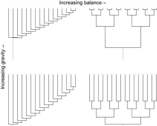
One means of determining whether extinction rates show the same age-dependent bias as speciation rates using tree shape is to look at the temporal distribution of internal nodes—a property of tree shape that we term “phylogenetic gravity” after center of gravity or center of mass as calculated for clade richness through time (Gould et al. Reference Gould, Gilinsky and German1987) (Fig. 1.) Phylogenetic gravity is driven by temporal differences in births and deaths (Pybus and Harvey Reference Pybus and Harvey2000). Low-gravity or “regressive” clades experience early bursts of diversification, causing most of their internal nodes in a phylogenetic tree to be distributed toward the root and the peak of their fossil occurrences to occur near their inception. High-gravity or “progressive” clades experience late bursts of diversification, causing most of their internal nodes to distribute toward the tips and their historical diversity to peak near the present. Additionally, however, the phylogenetic location of speciation and extinction events will also have an impact on gravity (Hagen et al. Reference Hagen, Hartmann, Steel and Stadler2015). For example, when birthrates and death rates are the same between evolutionary scenarios, if speciation and extinction rates are opposing on equivalent parts of the tree (as would be the case in the DE scenario), we would expect gravity to be higher than if they were equal (such as in the Pan scenario), because in the former scenario tips will be removed where there are few recently added tips, which increases the likelihood of loss of deep internal nodes. To date, however, most modelers of tree growth have focused on imbalance rather than gravity due to the relative scarcity of time-calibrated phylogenies (Purvis et al. Reference Purvis, Fritz, Rodríguez, Harvey and Grenyer2011).
The two dimensions of phylogenetic tree shape for a 16-tipped tree: balance and gravity, a new term we coin after “center of gravity.” Trees with most nodes toward the tip of the tree would be more likely to fall over (high center of gravity), whereas tips toward the root would be less likely to topple (low center of gravity).

Here, we test how different models of evolution, each with different implications for the origin of living fossils, affect the shape of the tree of life. As there is no agreed-upon definition of the living fossil, our aim is to take a particular phylogenetic concept for what living fossils might represent and test its self-consistency and utility for partitioning biodiversity. Because the majority of groups described as living fossils are often distinct lineages with few close relatives (Eldredge and Stanley Reference Eldredge and Stanley1984), we used the ED metric—the number of closely related species measured by phylogenetic isolation—as a simple proxy for living fossilness. For the living fossil concept to have general applicability, some or all of these low-diversity or evolutionarily distinct lineages must behave in similar ways over macroevolutionary time, as we would demonstrate if we discovered a strong signal for either a DE or Pan scenario. To this end, we developed a tree-growth model with age-dependent bias for speciation and extinction rates using a tip’s ED value. An ED bias is equivalent to an age-dependent bias, because time since last speciation correlates with a tip’s ED value. With this model we simulated 10,000 trees under different scenarios by varying the bias in rates of speciation and extinction by the ED of tips. To identify which hypothesis (DE, Pan, Hyd, or others) best recreates empirical evolutionary patterns, we compared simulated trees with more than 2000 empirical modern-day phylogenetic trees representing sections of the tree of life, using both phylogenetic imbalance and a birth–death independent measure of phylogenetic gravity.
Materials and Methods
Evolutionary Distinctness Biased Markov Model (EDBMM)
We developed a tree-growth model based on the equal-rates Markov model (ERMM) that biases speciation and extinction rates by the “living-fossilness” of a species—the EDBMM. The ERMM starts with a seed tree and adds and drops tips at random per unit branch length given birth (b) and death (d) parameters. The EDBMM biases selection for speciation or extinction by a tip’s ED value. At every time step (t), the ED values of all the tips are calculated, and these are used to bias the random selection of tips for speciation and extinction. Tips are then added or dropped, and the branch lengths of all extant tips are extended by
 ${t \over n}$
, where n is the number of tips in the tree, so that birthrates and death rates are constant in time. A simulation can be stopped after a set time has elapsed or the tree has reached a set number of tips (Supplementary Fig. S1).
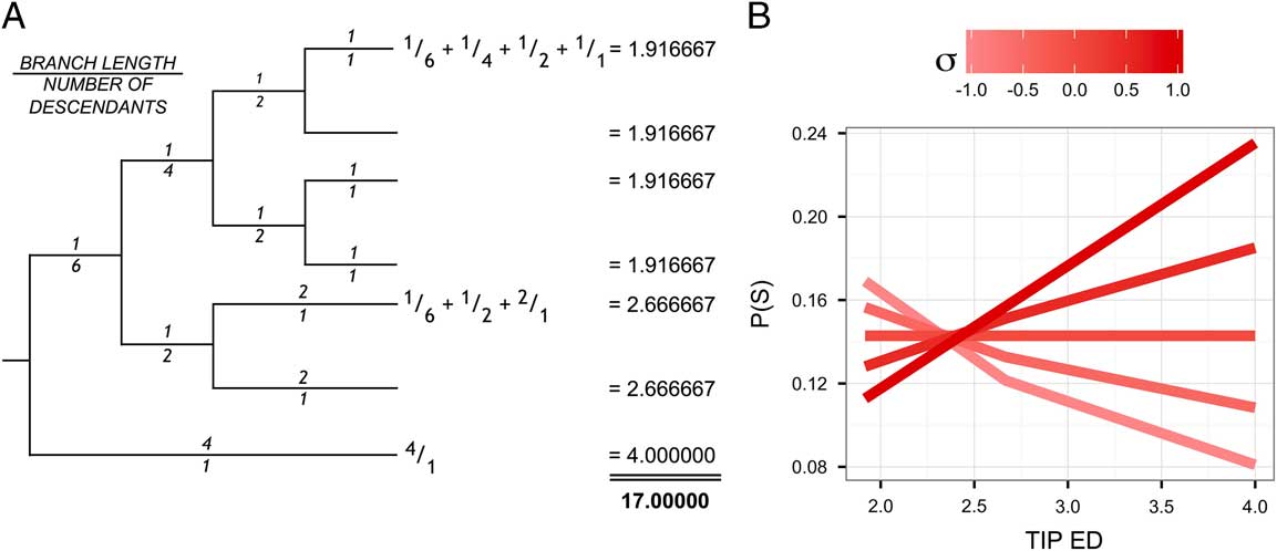
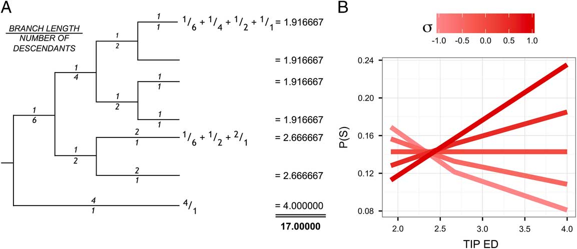
Because there is no fully agreed-upon definition of a living fossil, we use, as a proxy, “a low diversity lineage over time”; this is applicable to most lineages described as living fossils (Eldredge and Stanley Reference Eldredge and Stanley1984). This living fossilness proxy was calculated using ED, as this is a measure of a species’ level of phylogenetic isolation, making it an estimate for species’ recent lineage diversification rate. We calculated ED using the metric of Isaac et al. (Reference Isaac, Turvey, Collen, Waterman and Baillie2007). This metric shares the total branch length of the tree between tips by equally apportioning branch lengths by the number of descendants. In this way it takes into account all branches and is conceptually intuitive (Fig. 2).
(A) How to calculate ED from a phylogenetic tree: divide every branch length by the number of descendants, sum these proportional branch lengths for every tip in the tree to calculate ED scores. The total of these scores equals the total branch length of the tree. (B) How different ED values impact speciation probability, S, in the next time step given different σ values for tree in A. Under an ERMM, in which rates of diversification are equal among tips (σ=0), all the tips have an equal chance of diversifying. This will maintain tree imbalance, as nodes with more descendant tips have a greater chance of diversifying, and gravity will remain at a midlevel provided birth and death parameters are equal. Modeling this same tree under an EDBMM will lead to, depending upon the model’s parameters, different outcomes. For example, under a Pan simulation (σ=−1), the most evolutionarily distinct tip (4.00000) will become ever more distinct, as it will have lower rates of speciation and extinction, while the tips with lower scores will be more likely to speciate and go extinct, extenuating tree imbalance and increasing tree gravity.
Although speciation and extinction rates are held constant and determined by birth and death parameters, the relative probability of a tip being selected for speciation or extinction is determined by its ED value and two power parameters: σ (sigma) and ε (epsilon). The relative probability of the i th tip (i) speciating (S) at each time step (where n is the number of tips in the tree and d is their ED values) is given by equation (1), while its probability of going extinct (E) is given by equation (2). Given these probabilities and global birthrates (λ) and death rates (μ), the probability of diversifying (D) for the i th tip in the next time step can be determined, equation (3).
 $$p_{i} \left( S \right)\,{\equals}\,{{d_{i}^{\rsigma } } \over {\mathop{\sum}\nolimits_{j{\equals}1}^n {d_{j}^{\sigma } } }}$$
 $$p_{i} (E)\,{\equals}\,{{d_{i}^{{\repsilon}} } \over {\mathop{\sum}\nolimits_{j{\equals}1}^n {d_{j}^{{\repsilon}} } }}$$
 $$p_{i}^{'} (D)\,{\equals}\,\rlambda \cdot p_{i} (S){\minus}\rmu \cdot p_{i} (E)$$
In other words, species with higher EDs (hereafter “ED species”) experience increased rates of speciation and extinction for positive values of σ and ε, respectively, and reduced rates of speciation and extinction for negative values. Values of 0 for σ and ε provide no overall bias toward ED species, making speciation and extinction rates random for all tips in the tree. (See Fig. 2 for a visual representation of how different σ values influence probability of speciation for a seven-tipped tree.)
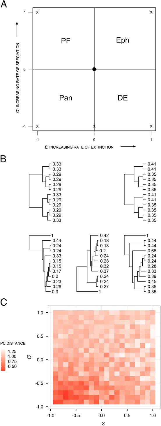
The σ–ε parameter space can be split into four quadrants, each with its own implications for the living fossil concept. We term each quadrant: “phylogenetic fuse” (PF, +σ, −ε), “dead-end” (DE, −σ, +ε), “ephemeral” (Eph, +σ, +ε) and “panchronic” (Pan, −σ, −ε). Additionally, we identify five scenario points representing the extremes of each quadrant and the “Hydra” (Hyd, σ=−1, ε=0) (see Fig. 3A). In the PF scenario, ED species have low extinction rates and high speciation rates, such that species that could be described as living fossils are “fuses” that will experience future evolutionary radiations. In the DE scenario, ED species have low speciation and high extinction rates; living fossils are evolutionary relicts doomed to disappear. In the Eph scenario, ED species have high speciation and extinction rates, making living fossils transient phenomena. In the Pan scenario, ED species experience low speciation and extinction rates, meaning that living fossils persist through time in low species numbers. In the Hyd scenario, ED species experience reduced speciation rates, but extinction rates are random, making living fossils potentially the products of both Pan and DE scenarios.
(A) σ–ε parameter space indicating the four quadrants for living fossils: PF, DE, Eph, and Pan. The point at 0,0 indicates an ERMM. The extreme values for each scenario are marked with “X”s. (B) Example 12-tipped trees, their expected shapes, and corresponding ED values for the five main simulation scenarios. PF and Eph produce balanced trees with moderate levels of gravity. Pan, Hyd, and DE all produce unbalanced trees but with different values for gravity, as demonstrated in the more distributed ED values as gravity becomes higher. (C) Distances of 0.1 × 0.1 grid cells of mean PC1 and PC2 values in simulated space to empirical trees. The smaller the value, the closer to empirical tree shape. Values generated from a PCA of the Colless, Sackin, and PSV metrics of simulated and empirical trees. Both PCs are weighted equally.

Tree Simulations
To determine which part of the σ–ε parameter space best recreates empirical tree shape, we simulated 10,000 trees using randomly generated σ and ε values between −1 and +1. We used seed trees of two tips and birth and death parameters of 2 and 1, respectively, and halted tree growth once they had reached a set number of tips determined by randomly selecting a value between 50 and 500 for each of the simulations. We also used the same parameters to generate 1000 trees for each of the extreme scenarios PF, DE, Eph, Pan, and the additional Hyd in order to compare the differences between these scenarios with larger numbers of trees.
In addition to exploring phylogenetic tree shape we also explored how idealized fossil records differed between Hyd, DE, and Pan. We took the simulated phylogenies generated from the extreme scenarios of Hyd, DE, and Pan, and their simulations were continued for twice the starting age of the initial tree using new birth and death parameters of 1 and 1 to remove the influence of a higher birthrate on clade shape. In this stage, extinct tips were not removed. One hundred equally spaced time samples were then extracted from the tree. Each sample recorded the number of descendants for each clade, excluding all tips that were either extinct or not yet extant before and after the time point. A clade was defined in the strict monophyletic sense as a node and all its descendants. This produced a species richness time series for every clade in the tree that accounts for both extant and extinct lineages, unlike other time series based on present-day phylogenetic trees (e.g., Pybus and Harvey Reference Pybus and Harvey2000). We calculated various clade statistics from these idealized fossil records, including the center of gravity/mass, which measures the relative time point when a clade reaches its peak (Gould et al. Reference Gould, Gilinsky and German1987), and center of gyration, which measures variance around that peak. Statistics were calculated for all clades with total sizes of more than 100 descendants after the 25th time point to reduce the influence of edge effects.
Empirical Tree Search, Manipulation and Comparison
Empirical trees were gathered for comparison with the simulated trees. We first identified large species-level phylogenies with more than 1000 taxa from the literature (see Supplementary Table S1). These trees were supplemented by downloading published phylogenies from TreeBase (Piel et al. Reference Piel, Donoghue and Sanderson2002) using the R package treebase (Boettiger and Temple Lang Reference Boettiger and Temple Lang2012). TreeBase searches were constrained to species-level phylogenies and to trees with more than 50 taxa. Trees that were polytomous were rendered fully bifurcating using the function multi2di (Paradis et al. Reference Paradis, Claude and Strimmer2004), because, upon inspection, the majority of these polytomies were due to inference error as they did not separate known taxonomic groups. Because this function randomly splits polytomies, we generated a distribution of 100 trees to account for any bias. Trees with branch lengths that were not ultrametric (i.e., branch lengths not relative to time) were converted by rate smoothing. To account for differences between rate-smoothing algorithms, we ran three different methods: D8 (Britton et al. Reference Britton, Anderson, Jacquet, Lundqvist and Bremer2007), MPL (Britton et al. Reference Britton, Oxelman, Vinnersten and Bremer2002), and PL (Sanderson Reference Sanderson2002). To make comparisons with the simulated trees, we ensured empirical trees had the same number of tips by reducing any tree with more than 500 tips by extracting nonoverlapping clades of between 50 and 500 tips. In total, we sourced 2061 empirical trees with a mean of 101 (25th, 50th, and 75th quantiles: 60.0, 78.0, and 110.5) tips (Supplementary Fig. S2). The mean year of publication of the empirical trees was 2009 (SD 4). Of these trees, 1432 (69%) were polytomous, 802 (39%) had given branch lengths, 64 (3%) were already ultrametric, and a mean 647 (31%), 492 (24%), and 370 (18%) were successfully made ultrametric using D8, PL, and MPL, respectively.
For all sourced empirical trees, the phylum, class, and order represented by each tree were identified using the online Global Names Resolver taxonomic tool (Global Names Architecture 2015). The 215,752 unique names in all of the sourced trees represented 32 phyla, 87 classes, and 260 orders. The number of trees represented by each phylum was highly unequal; the top five phyla—Tracheophyta, Ascomycota, Chordata, Arthropoda, and Basidiomycota—represented 85% of all trees (Supplementary Fig. S3). Sixty-one trees had names that could not be identified at the phylum, class, or order rank.
For empirical and simulated trees we calculated “shape metrics” for both imbalance and gravity. To avoid pseudoreplication, in cases in which empirical tree data were available as distributions of trees rather than single trees—as produced from Bayesian analysis or by randomly removing polytomies—shape statistics were calculated for each tree in the distribution, and the mean value was used in subsequent analysis.
To estimate imbalance we used both Colless (Reference Colless1982) and Sackin (Reference Sackin1972) metrics. As imbalance metrics are affected by the number of tips in a tree, both measures were normalized with the expected value for a pure-birth tree of the same number of tips (“Yule normalization”) (Mooers and Heard Reference Mooers and Heard1997). Values greater than 0 indicate a tree that is more unbalanced than the Yule reference, and values less than 0 indicate a tree that is more balanced. These metrics were calculated and normalized using the functions of the R package apTreeShape (Bortolussi et al. Reference Bortolussi, Durand, Blum and François2006).
γ (gamma) (Pybus and Harvey Reference Pybus and Harvey2000) is used as a measure of gravity (termed “tippiness” by Manceau et al. Reference Manceau, Lambert and Morlon2015). However, γ was originally devised to measure stable (γ=0), increasing (γ>0) or decreasing (γ<0) lineage generation through time and is therefore sensitive to differences in birth–death parameters between trees—a factor we cannot control when sourcing empirical trees. Therefore, in addition to γ, we also calculated phylogenetic species variability (PSV) (Helmus et al. Reference Helmus, Bland, Williams and Ives2007) as a measure of phylogenetic gravity. As a measure of the relative distance between tips, PSV negatively covaries with gravity. Star trees, in which all tips are equally distant, have low gravity and PSV values of 1. “Dot” trees or “line” trees, in which tips are separated from a single distant tip and internal nodes clustering, have high gravity and PSV values tending toward 0 (Supplementary Fig. S4). Although originally developed as a measure of community phylogenetic diversity, we show in supplementary analysis (see Supplementary Figs. S5, S6) that PSV is less sensitive to the birth–death parameter (Pearson’s R: −0.27 and 0.78, for PSV and γ, respectively) and more sensitive to ε (Pearson’s R: 0.20 and −0.13, for PSV and γ, respectively) when birth–death varies randomly.
Normalization was not required for gravity, as the metrics we use are independent of age and number of tips of the tree. Gravity metrics, however, require trees to be ultrametric, and as such only the ultrametric empirical trees (18–31% of sourced trees for the different rate-smoothing methods) were compared with simulated trees using gravity metrics. Because gravity and imbalance metrics partly correlate, we performed principal component analysis (PCA) using Sackin, Colless, and PSV metrics to map the distances of empirical and simulated trees in “tree shape space.”
All of the methods described above were run in the R environment (Version 3.2.3) and can be reproduced using online R scripts and functions, available via GitHub (Bennett Reference Bennett2016).
Results
Simulated Trees
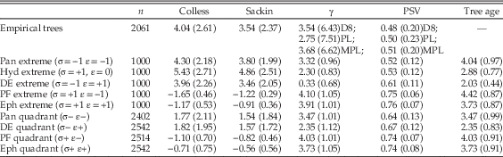
We found strong differences between the 10,000 simulated trees in each of the four quadrants of σ–ε parameter space. There was a strong negative correlation between σ and imbalance for both Colless and Sackin metrics (Pearson’s R: −0.80 and −0.78, respectively; Supplementary Fig. S7). As such, the scenarios that represent positive σ in σ–ε space, PF and Eph, both produced trees more balanced than the Yule equivalent (Table 1). Because all empirical trees are less balanced than the equivalent Yule tree, we consider these scenarios to be implausible. Pan, Hyd, and DE scenarios, however, represent negative σ in σ–ε space and produced trees more unbalanced than the equivalent Yule tree, consistent with empirical trees (Table 1).
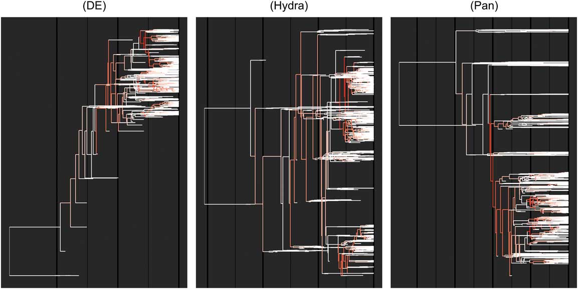
We found no significant differences between each of the four quadrants in terms of gravity, except for the DE scenario, which produced trees with significantly lower γ values than all other simulated trees (37% lower, t-test: p<0.001) and empirical trees (34% lower using D8, t-test: p<0.001). Because ED species have negative speciation and extinction rates in the DE scenario, the most isolated branches of the tree are more likely to be pruned. This leads to the constant shrinking of the tree from the base, and causes the γ value to be low despite a birth–death parameter of 2 to 1. We term this the “shrinking tree problem” (see Fig. 4). This explanation was corroborated by the average age of trees simulated in the DE quadrant being significantly lower than all other simulated trees (26% lower, t-test: p<0.001).
Chromatophyla of trees with fossil taxa produced under the three most likely scenarios of ED-biased evolution: DE, Hyd, and Pan. Darker branches indicate greater numbers of descendants; darker areas of the tree indicate points of diversification. Under the DE scenario, the resulting tree without fossils is younger than the equivalents under both Pan and Hyd due to the pruning of ED tips—the shrinking tree problem. The DE tree’s most distinct branches are extinct; the Pan tree’s ED branches are all extant and the tree is as old as the simulation time span. (See online for color version.)

Across all estimates of PSV, differences between each of the quadrants were not great, although Pan had the lowest PSV values, indicating higher gravity. In particular, PSV values were lowest for simulations with negative σ and midranging or negative ε (Supplementary Fig. S8). When excluding trees simulated with positive σ values, we found weak negative correlations between gravity and ε (Pearson’s R: 0.18 [PSV] and −0.53 [γ]; Supplementary Fig. S9).
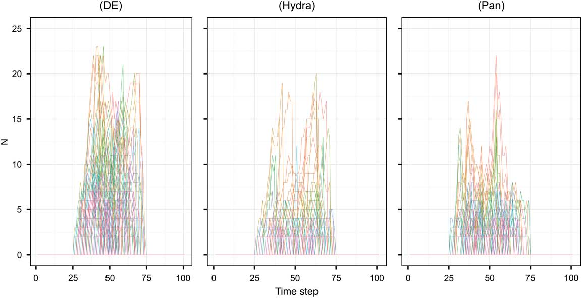
The clade dynamics show different shapes between the three extreme scenarios: DE, Hyd, and Pan. Although Pan produced trees with higher phylogenetic gravity than both DE and Hyd, the mean clade center of gravity was lowest (Table 2). Pan also produced the most clades, which on average lasted less time than clades of other scenarios, indicating a high turnover. Furthermore, Pan had the highest gyration, indicating that although its clades tended to peak closer to the midpoint of their time span, this peak was more plateaued than in DE and Hyd. DE produced the fewest number of clades and had the highest gravity, indicating relatively fast clade extinction. With random extinction, clades produced with Hyd contained on average more species at peak (Table 2, Fig. 5).
Clade dynamics between the 25th and 75th time intervals for the 100 largest clades produced by exemplary simulations of the DE, Hyd, and Pan scenarios. Each clade trajectory through time has a different color. (See online for color version.)

Empirical Trees
Empirical trees were more unbalanced than the Yule equivalent for both Colless and Sackin metrics, 4.0 (SD 2.6) and 3.5 (SD 2.4), respectively. We did not find significant differences between γ generated with each of the three rate-smoothing methods (t-testD8~PLl: p=0.062, t-testD8~MPL: p=0.750; referred to later as γD8, γPL, and γMPL). The mean γ for empirical trees was greater than expected for a simulated tree where birth and death parameters are equal, implying increasing lineage generation for most trees (Table 1). We also found no significant differences between PSV values generated from each of the three methods (t-testD8~PL: p=0.59, t-testD8~MPL: p=0.34; referred to later as PSVD8, PSVPL, and PSVMPL). The PSV values were midranging, indicating a midlevel gravity for most trees (Table 1). Although we found significant correlation between gravity and imbalance (Pearson’s product moment correlation, Colless~PSVD8: R=−0.21, p<0.001), we deem this to be due to the physical impossibility of a tree with low gravity and high imbalance. We found significant differences between taxonomic groups at all three taxonomic ranks for both imbalance metrics but not for either of the gravity metrics (Supplementary Table S2). The variance of shape metrics was larger between orders than between either classes or phyla, which may indicate that lower-ranked groups have diverging macroevolutionary dynamics compared with higher ranks (Supplementary Figs. S10–S12). For example, the variance of the means between taxonomic groups of Sackin and PSVD8 metrics increased 111% and 494%, respectively, from phyla to orders. However, we found that this increase in variance, or for any of the other metrics, was not significant (permutation tests of variances of the means from phyla to orders: p=0.89 and p=0.76 for Sackin and PSVD8, respectively) (Supplementary Table S2).
Empirical and Simulated Compared
In terms of imbalance, Pan and DE quadrants were both equally near to the empirical trees. However, for gravity as measured by PSVD8, the Pan quadrant was closer to the empirical than DE (Table 1). To explore intraquadrant differences, we plotted the distances of each 0.1 × 0.1 grid cell in σ–ε space to empirical trees for Colless, Sackin, and PSVD8 metrics (Supplementary Fig. S13). Visually, this shows that simulated trees with extremely low values of σ and mid- or negative levels of ε produce trees most similar to empirical trees in terms of imbalance and gravity. With a PCA of Sackin, Colless, and PSVD8 for the simulated and empirical trees, we found the grid cells closest to empirical trees mostly fell within the Pan quadrant (Fig. 3C).
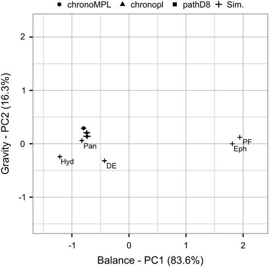
This was further corroborated by a PCA of empirical trees and the simulated trees of each extreme scenario, which shows Pan to be closer to empirical trees in principal component (PC) space than both of the other −σ scenarios, Hyd and DE (Fig. 6). However, the level of variance in empirical tree shape was not matched by any of the simulated scenarios, particularly in gravity metrics (see Table 1). This higher variance in gravity could be the result of a greater diversity of birthrates and death rates; repeating the PCA above with empirical trees partitioned into γ>0 and γ<0 showed that empirical trees that are likely to have experienced reduced or negative diversification rates are closer in PC space to DE and Hyd scenarios (Supplementary Fig. S14). Additionally, we found a strong difference between the trees sourced from the literature, which had lower gravity than all simulated trees, than those originating from TreeBase (Supplementary Fig. S15).
PCA of trees simulated using the extreme scenarios and empirical trees using Yule-normalized Colless and Sackin and PSV. Error bars are standard errors. The three points for empirical trees represent the trees produced using different rate-smoothing methods. PC1 correlates with Sackin and Colless and PC2 correlates most with PSV, making the two PCs equivalent to imbalance and gravity dimensions of tree shape.

Mean (and standard deviation) tree shape statistics for empirical and simulated trees in different quadrants and points of σ–ε parameter space as indicated by Fig. 3A.

Mean (and standard deviation) clade shape statistics for 3000 simulated trees in three points of σ–ε parameter space as indicated by Fig. 3A. All statistics are calculated for clades representing more than 100 species between the 25th and 75th time intervals. No. of clades, total number of clades; Gravity, center of gravity/mass; Gyration, center of gyration; t, clade time span; Peak spp., peak diversity; Total spp., total number of species throughout time span. *Gyration E-2.

Discussion
Our phenomenological model of tree growth uses a tip’s ED value to bias speciation and extinction rates to test the reality of the living fossil. With our model, we confirm the results of previous studies in which younger or more diverse clades have higher rates of net speciation (Purvis et al. Reference Purvis, Fritz, Rodríguez, Harvey and Grenyer2011; Hagen et al. Reference Hagen, Hartmann, Steel and Stadler2015; Rabosky and Goldberg Reference Rabosky and Goldberg2015) by showing that scenarios in which ED species have increased rates of speciation lead to trees with greater phylogenetic balance than in empirical trees. Scenarios in which ED species have reduced rates of speciation (DE, Hyd, and Pan) all produced levels of imbalance similar to empirical trees. Of these three scenarios, however, we found that the Pan scenario, in which speciation and extinction rates were reduced for ED species, produced trees closest in both gravity and imbalance to empirical trees. By eliminating the Hyd hypothesis, we therefore show that the living fossil label represents a true grouping, and by eliminating the DE hypothesis, that it does not merely represent “evolutionary relicts” of once-large radiations that are soon to go extinct (Nagalingum et al. Reference Nagalingum, Marshall, Quental, Rai, Little and Mathews2011). Instead, ED species are generally the product of the same macroevolutionary phenomenon and can therefore be grouped as a “real category” of biodiversity and are able to persist without speciating or going extinct for long periods of time.
Although our approach was only able to work with a purely phylogenetic interpretation of the living fossil based on ED, our results reveal this proxy more closely recalls the original living fossil concept proposed by Darwin (Reference Darwin1859) as a “window into the past” than more recent concepts of living fossils as evolutionary dead-ends.
Our results differentiate between the fit of each of our three main hypotheses (Pan, Hyd, and DE) to the shape of the tree of life in terms of phylogenetic gravity. While these results might theoretically be contingent on methodological particulars (metrics of gravity and rate-smoothing methods employed and empirical tree sampling), we have good reasons to infer that this is not the case. First, although PSV has never been used in this capacity before, it is still a useful measure of the shape of a tree, as it indicates whether the tree is more like a star or a line and is therefore equivalent to a metric of gravity. In supplementary analysis in which we simulated trees with varying birth and death parameters, we demonstrated that PSV, although still strongly correlating with the birth parameter, also correlates more with ε than γ does. For this reason, we favored PSV over γ for comparisons of gravity, because the differences in γ between and among empirical trees were much greater than that produced by our simulations, obscuring any signal. Second, several rate-smoothing methods were employed, and all produced similar results. Additionally, we recovered the same tendency for empirical trees to have high levels of gravity (γ>0 and PSV ~ 0.5) in trees that did not require rate smoothing (i.e., were already ultrametric). We did, however, find significant differences between trees sourced from the literature and those from TreeBase. We were unable to break up the empirical trees based on the methods used to create them due to the lack of readily available data. Doing this, we may have found further sources of bias that can impact tree shape, and therefore concede that this may be a weakness in our estimation of mean gravity of empirical trees. Third, the higher levels in gravity for empirical trees might reflect a bias in the sourced data toward groups in the process of radiating. We think it unlikely that this is the case, however, as we sampled from a broad range of taxonomic groups. Furthermore, our results indicate that the range of PSV values for radiating and nonradiating clades (i.e., the PSV values for those trees with positive and negative γ) are still greater than those produced by the Hyd or DE scenarios; the ratio of higher births to deaths alone is unable to generate the higher gravity seen in empirical trees.
Although our results indicate that extinction rates show negative age dependence, there is little evidence for this from the fossil record. Most notably, Van Valen’s Red Queen hypothesis (Van Valen Reference Van Valen1973) was proposed on the discovery that extinction rates appeared to be independent of lineage age for a range of taxonomic groups. Boyajian (Reference Boyajian1991) corroborated this by showing that extinction rates were independent of lineage age even during periods of mass extinction for fossil marine families. More recently, Ezard et al. (Reference Ezard, Aze, Pearson and Purvis2011) showed that extinction rates were more influenced by environmental factors in foraminiferans, rather than biotic factors such as relative clade size. Such evidence would point to a Hyd scenario of evolution instead of a Pan scenario. However, in some instances extinction rates have been found to demonstrate positive age dependence. Quental and Marshall (Reference Quental and Marshall2013) demonstrated that an island biogeography model of clade rise and fall could explain the trajectories of recently extinct mammalian orders, a process akin to the DE scenario. Additionally, Wiltshire et al. (Reference Wagner and Estabrook2014) developed a new method for measuring age dependence in extinction rates and found that foraminiferans all showed positive age dependence.
Given this fossil evidence, how can we assert our claim that extinction rates show negative age dependence as per our results? We would suggest that there are multiple factors determining extinction rates, which are generally independent of lineage age and its correlate, ED. A Pan scenario, however, can be recreated with only the most evolutionarily distinct lineages, which represent a small subset of total biodiversity, having reduced extinction rates. Indeed, as a Pan model continues to run, the relative skew of ED continues to grow, making the less evolutionarily distinct tips of the tree have random extinction with respect to one another. Statistically detecting such a nonlinear relationship for a small subset of the most evolutionarily distinct species from the fossil record would be difficult. However, by taking a tree-growth modeling approach, we demonstrate how Hyd and DE scenarios are implausible general models of evolution. Both Hyd and DE scenarios lead to the continual reduction in tree age due to the loss of the most evolutionarily distinct branches—the “shrinking tree problem.” Only a Pan model of evolution can recreate highly evolutionarily distinct lineages such as horseshoe crabs, ginkgos, and tuataras while maintaining tree imbalance. Trees produced with the Hyd and DE scenarios had, respectively, a third and a half less the age of Pan trees, which would make the persistence of such isolated lineages highly unlikely through geological time. Slowly evolving, species-poor lineages are required to maintain the age of a tree.
In Raup’s (Reference Raup1985) terminology, our modeling framework fits into a time-inhomogeneous category because, although the global parameters of speciation and extinction remained constant, the relative rates differed between clades as a function of the proportion of evolutionarily distinct species each clade represented. By placing differential rates of diversification on potentially competing clades, our modeling approach is related to the density-dependence logistic models of Raup (Reference Raup1985), Sepkoski (Reference Sepkoski1978, Reference Sepkoski1979, Reference Sepkoski1984), and others. Furthermore, different scenarios resemble the simulations of previous modelers. The DE scenario that causes the sharp rise and fall of clades as a result of increasing and decreasing extinction and speciation rates respectively for older clades is most related to the island biogeography model of clade rise and fall of Quental and Marshall (Reference Quental and Marshall2013). The Hyd scenario that modifies speciation rates and keeps extinction rates constant is akin to the coupled logistic models of directly competing clades (Miller and Sepkoski Reference Miller and Sepkoski1988; Roy Reference Roy1996; Sepkoski et al. Reference Sepkoski, McKinney and Lidgard2000). Despite these similarities, the differences in process from our approach should be highlighted: these models generally attempt to explain taxonomic diversity against time, whereas our simulations modeled phylogenetic trees, and we make no explicit assumptions about the roles of biotic or abiotic forces shaping diversity nor do we attempt to capture potential competition (see review by Voje et al. Reference Voje, Holen, Liow and Stenseth2015).
Gould et al. (Reference Gould, Gilinsky and German1987) found clades tended to be bottom-heavy or “regressive” for a wide range of taxonomic groups. All of the clades in our simulations were top-heavy, although Pan produced the least top-heavy clades. Our results, however, are not directly comparable to those generated from the fossil record. This is due to differences in how a clade is defined between our analyses and in the fossil record. We used a strict monophyletic definition because we were working with phylogenetic trees rather than simulating morphological shifts; those working on the fossil record do not have access to full phylogenetic information and have hence preferred a morphological paraclade/clade definition. In Raup’s (Reference Raup1985) terminology we used a phylogeneticist approach, while Gould et al. (Reference Gould, Gilinsky and German1987) used an evolutionary taxonomist approach. We would therefore expect to calculate higher estimates of center of gravity in our simulated clades with respect to the results of Gould et al. (Reference Gould, Gilinsky and German1987), because the phylogeneticist approach counts all descendants from a node, while the evolutionary taxonomist approach would only count those descendants deemed to still be part of the higher clade. Furthermore, the phylogeneticist approach should always lead to top-heavy estimates of gravity due to double counting as a result of the hierarchical nature of a tree: for every diversifying node there is a parent node, yet for every node soon to go extinct there are no child nodes. For these reasons we argue that the clade trajectories of the Pan scenario most closely match those found in the fossil record.
It should be stressed, however, that we have not set out to develop a “general model of evolution.” We set out to determine what biases in diversification with respect to ED best reproduce observed phylogenetic trees. Factors other than ED and its correlates may prove to be more important in shaping other macroevolutionary patterns. For example, the high variance in γ in empirical trees—a factor none of our simulations were able to recreate—may reflect the importance of adaptive radiations (Simpson Reference Simpson1944). Indeed, unexpectedly high levels of imbalance have previously been used to identify adaptive radiations (Purvis et al. Reference Purvis, Fritz, Rodríguez, Harvey and Grenyer2011). Excluding the signal generated by radiations, however, indicates that turnover—speciation and extinction without net gain or loss in species number—is the secondary key process. Alfaro et al. (Reference Alfaro, Santini, Brock, Alamillo, Dornburg, Rabosky, Giorgio and Harmon2009) found that up to 85% of present-day vertebrate species could be the result of adaptive radiations, with the remaining 15% the result of turnover. Turnover has been noted in the fossil records of many major clades, for example, Carnivora (Liow and Finarelli Reference Liow and Finarelli2014). The Pan scenario is essentially a turnover process, as tips have the same rate of speciating or going extinct, with these rates being determined by ED values. Turnover alone is able to explain the phenomenon of high values of γ despite trees as a whole not experiencing higher births to deaths (Boettiger and Temple Lang Reference Boettiger and Temple Lang2012), as typically seen in the fossil record (Alroy et al. Reference Alroy2008). Lineages with high turnover will continually add new nodes toward the tips, while lineages with low turnover will maintain tree age and provide few nodes toward the root.
ED is an increasingly accepted proxy for the living fossil. Cavin and Kemp (Reference Cavin and Kemp2011) used it to identify lungfish as the most evolutionarily distinct vertebrate species—much more so than coelacanths—and recommended them for the living fossil tag. ED, however, is only a proxy for the living fossil, as it cannot capture all elements of the living fossil concept, most notably “little change through time” (Eldredge and Stanley Reference Eldredge and Stanley1984). Regardless of scenario (Pan, Hyd, or DE), under a Brownian motion model of character evolution we would expect ED species to be more ecologically and morphologically distinct, as they have the greatest evolutionary distance from other species (Isaac et al. Reference Isaac, Turvey, Collen, Waterman and Baillie2007). Few studies have been performed to investigate this question. Although Redding et al. (Reference Redding, DeWolff and Mooers2010) showed that high ED primates were “odder” compared with low ED primates, this appears not to be the case from the fossil record when considering lineage ages and character states. Older lineages of fossil crinoids have been found to be less morphologically distinct than younger lineages (Liow Reference Liow2004), and trachyleberidid ostracodes were found to be morphologically equivalent between older and younger lineages (Liow Reference Liow2006). Wagner and Estabrook (Reference Voje, Holen, Liow and Stenseth2014) showed that paired character traits across a wide range of fossil groups and periods showed hierarchical stratigraphic compatibility: character states show morphological progression through the loss of earlier states. It could be argued that species that may still retain these “primitive” character states as they disappear globally are more likely to be evolutionary distinct as they are less likely to produce future progeny. Under a punctuated equilibrium model of evolution in which most character evolution occurs during speciation events (Gould and Eldredge Reference Gould and Eldredge1993), only a Pan scenario would recreate the morphological primitiveness of living fossils, as it would generate high ED species through long periods of low diversification rates rather than recent rapid extinction. There is recent evidence that speciation events do indeed accelerate such change (Venditti and Pagel Reference Venditti and Pagel2010; Ezard et al. Reference Ezard, Thomas and Purvis2013). Furthermore, recent pan-vertebrate genomic analyses of protein-coding sequences and genomic rearrangements indicate that species commonly identified as living fossils do experience reduced rates of change (Amemiya et al. Reference Amemiya2013; Venkatesh et al. Reference Venkatesh2014).
Regardless, we do not suggest that ED species equate to living fossils under all possible definitions. By demonstrating that positive feedback in diversification rates is required for producing the observed shape of the tree of life, we show that evolutionary performance is unequally distributed and that living fossil as a label can have more meaning than just the tail end of a normal distribution. It can be used to describe a true grouping of lineages with substantially lower rates of diversification than seen in other parts of the tree of life, rates that are reflective of the HCD itself, and that represent an emergent feature of a turnover-based model of evolution. Our aim was not to determine what the processes are that allow living fossils to arise but to validate or invalidate potential definitions of the living fossil. By demonstrating the validity of a panchronic definition, we hope to have opened the door for future research that seeks to determine what these processes may be.
Acknowledgments
Thanks to A. Purvis, L. Signorile, S. Dures, M. Bennett, and K. A. Jønsson for useful initial discussions; to L. H. Liow for introducing the term “panchronic”; and to P. Wagner and an anonymous reviewer whose insightful comments and suggestions have greatly improved this article.
Supplementary Material
Data available from the Dryad Digital Repository: http://dx.doi.org/10.5061/dryad.hm55b