

1. Introduction
1.1. In this paper we are concerned with measuring the costs of adverse selection in a long-term care insurance (LTC) market, where there are multiple sources of adverse selection. In order to provide some quantitative measure into the debate over the use of genetic tests in insurance underwriting, we will estimate the relative impact of genetic information as one of these sources.
1.2. We will use multiple state Markov models to represent the LTC market with states indicating health status, whether genetic test has been taken and whether the life is insured. These will be parameterised in part using transition intensities from relevant previous studies, as well as making use of available data from prospective cohort studies to fit transition intensities ourselves. For the purpose of illustrating the relative impact of sources of adverse selection, we do not consider the compatibility of data sources to be a concern, as we use them to provide us a baseline for modelling health. From this baseline, we can observe the order of magnitude of the adverse selection costs from each source and allow us to understand how they interact. As with any model, careful consideration should be given over the appropriateness before applying our models to any other purpose.
1.3. In section 2 we describe the LTC product and review previous models of long-term care.
1.4. LTC is a product to pay for old-age care, so our modelling will commence with detailing a model for old-age health in section 3. This will involve estimating transition intensities between states in a Markov model. We will also introduce and parameterise an intermediate state for dementia, where the life has noticed the initial signs of the disease but a lack of clinical diagnosis creates an information asymmetry and hence an opportunity for adverse selection.
1.5. Under an LTC contract, benefit payments may depend on path taken by the insured through the health model. In order to approximately calculate the expected present values of future benefits at the start of each calendar year of a policy’s existence, in section 10 we specify a model to simulate future lifetimes and the resulting LTC cashflows.
1.6. Previous actuarial models of genetic adverse selection have assumed an established insurance market. In such markets, premiums have already absorbed the cost from an increased proportion of high-risk lives, and we merely find by what factor they are larger than if there was no adverse selection. As we are considering a start-up market, we will assume that insurers initially have insufficient experience to set premiums appropriately. As they gain experience, they will compare actual cashflows with what was expected, and respond to differences by changing premiums chargeable to new business. In this way, we make the premium rates dynamic. As the premiums adjust, so will the costs of adverse selection and our model will be able to chart these costs over time. This methodology, where we explicitly model the emergence of information and its relation to adverse selection costs, could also be applied to an established market where a new source of adverse selection is being introduced. In section 5 we will set out a model for a start-up insurance market. In this market model, we will describe how we will use the expected present values calculated from our simulations in order to calculate our dynamic premium rates.
1.7. A recent UK government proposal to limit the costs faced by individuals when paying for care has brought attention to long-term care. It has also brought suggestions of a role for insurance companies in transferring some of the remaining risk from individuals. In section 6 we review the LTC market in the United Kingdom.
1.8. We parameterise benefits based on the cost of care provision in the UK and include a government proposal to limit the individual’s liability for their care costs in section 7.
1.9. In section 8 we analyse the premium rates chargeable over time assuming underwriters have full access to information regarding the health of the customer. From this analysis we determine appropriate scenarios to run through in section 9, calculating adverse selection costs over time. We will also assess what impact the government’s proposed cap on care costs has on adverse selection costs under our modelling assumptions.
1.10. In the European Union there is a requirement for premiums to be equal for males and females. In section 10 we analyse the cross-subsidy inherent in unisex premiums when there is adverse selection in the market.
1.11. Finally, in section 11 we present our conclusions and suggest where further work may be useful, given the direction of research in the genetics field.
2. LTC
2.1. LTC provides the policyholder with a benefit to cover the cost of payments to a carer or care home. There are two main reasons for requiring care: reduced functional ability and reduced cognitive function (dementia). We will start by describing these causes, then review previous models of long-term care.
2.2. Functional Ability
2.2.1. We measure reduction in functional ability in terms of activities of daily living (ADLs), e.g., the Barthel and Katz indices (Mahoney & Barthel, Reference Mahoney and Barthel1965; Katz et al., Reference Katz, Downs, Cash and Grotz1970) and instrumental activities of daily living (IADLs) – these are not as fundamental as ADLs but still necessary to retain one’s independence – that can no longer be performed. The ADLs used to trigger an insurance claim are typically needing assistance with at least two of bathing, dressing, toileting, transferring, continence or feeding. We use the same language as is used among insurers to describe the level of disability:
a. a person that has problems performing x ADLs is said to have xADLs;
b. a person that can perform all ADLs is said to have no ADLs.
2.2.2. Once functional ability has been lost, it is not necessarily permanent and lives can recover to healthier states. In this way it is similar to income protection insurance and much like income protection, a desirable feature from an insurer’s perspective may be a deferred period to prevent the high cost of claims underwriting when the claimant does not require a long period of care.
2.3. Cognitive Function
2.3.1. Dementia is an umbrella term for a group of disorders that impair cognitive function by affecting thought processes, memory, judgement and personality. Although the main sufferers are the elderly, some diseases occur at younger ages. It is progressive, so symptoms gradually worsen but sufferers may show these symptoms inconsistently: they may have periods of lucidity despite severe progress of the disease. As it progresses and the sufferer loses the ability to take care of himself/herself, informal care from family members or formal care in a nursing home may be necessary.
2.3.2. We class the causes of reduced cognitive function into two groups: dementia owing to Alzheimer’s disease (AD) and dementias that are not caused by Alzheimer’s disease (non-AD).
2.3.3. The main type of dementia is AD, which is responsible for 65%–70% of cases (Berr et al., Reference Berr, Wancata and Ritchie2005). Its causes are not known but it is thought to have a strong genetic component; Gatz et al.(Reference Gatz, Reynolds, Fratiglioni, Johansson, Mortimer, Berg, Fiske and Pedersen2006) estimates that between 60% and 80% of the risk is genetic.
2.3.4. There are two distinct varieties of AD, named for the timing at which they occur: early-onset AD, which usually affects lives aged <60 years old and late-onset AD, the more common form that affects lives aged 60 years and older. As we are concerned with post-retirement care, we are only interested in late-onset AD. Therefore, when we refer to AD, this is specifically the late-onset variety. Varieties of non-AD include, but are not limited, to vascular dementia (the most common form of non-AD and also known as multi-infarct dementia), dementia with Lewy bodies, Parkinson’s disease and Huntington’s disease. There is a great deal of overlap in the symptoms of AD and non-AD, so diagnosis can only be made with certainty at autopsy, where the brain may be properly analysed.
2.3.5. The genetics of AD is not fully understood and the only gene known to affect its development, which has sufficient epidemiology for modelling purposes, is the apolipoprotein E gene (APOE). Coon et al. (Reference Coon, Myers, Craig, Webster, Pearson, Lince, Zismann, Beach, Leung, Bryden, Halperin, Marlowe, Kaleem, Walker, Ravid, Heward, Rogers, Papassotiropoulos, Reiman, Hardy and Stephan2007) established APOE as “the major susceptibility gene” for late-onset AD. In the advent of genome-wide association studies, identification of potential susceptibility genes has picked up pace and there have been many candidates for association with late-onset AD. The progress of the research is reviewed in Alagiakrishnan et al. (Reference Alagiakrishnan, Gill and Fagarasanu2012), listing four additional susceptibility genes for which results have been replicated: phosphatidylinositol-binding clathrin assembly protein, clusterin, complement receptor 1, B1N1 and GRB2-associated-binding protein 2 genes.
2.4. Previous Models of Long-Term Care
2.4.1. Here we summarise the methodology and the aims of some of the models of long-term care in the United Kingdom. The major difference between the methodologies is with regards to the use of either transition intensities or prevalence rates.
2.4.2. The first studies we consider used a transition intensity-based approach. Transition intensities are a more fundamental quantity than prevalence rates – with transition intensities into and out of a state, one can calculate prevalence at any given time. The benefit of using transition intensities is that they allow greater flexibility in the modelling – the prevalence of diseases can change overtime and using transition intensities enables this to be modelled. However, they are more difficult to estimate – whereas prevalence requires only a snapshot of a population at one point, to estimate transition intensities, we need to understand how the population changes over time. Ideally, such an exercise would involve revisiting the population at a later time to find the details of any changes in health, increasing the cost and duration of analysis.
2.4.3. Macdonald & Pritchard (Reference Macdonald and Pritchard2000) set out a Markov model for the onset of AD dependent on the APOE variants carried by the life. They use this model in Macdonald & Pritchard (Reference Macdonald and Pritchard2001) in the context of an established market for LTC to calculate potential adverse selection costs from high-risk genotypes buying at an increased rate. Adverse selection cost was calculated as the percentage increase in premiums after increasing the proportion of lives of high-risk genotypes among those who buy the contract.
2.4.4. Pritchard (Reference Pritchard2006) fitted a Markov model for disability with five levels of functional disability to the results of the National Long-Term Care Study in Manton (Reference Manton1988). His aim was to estimate the costs of disability claims in an LTC contract. He calculated the expected present value of the benefits attributable to occupancy of each state and found that where studies exclude recovery, they could substantially overstate the cost of benefits.
2.5. Colgan (Reference Colgan2006) updated Macdonald & Pritchard’s (Reference Macdonald and Pritchard2001) model using data from the Consortium to Establish a Registry for Alzheimer’s Disease (CERAD) to estimate transition intensities after the point of AD onset (mortality and institutionalisation). He used his model to analyse the impact of medical treatments for AD on the costs of long-term care.
2.5.1. Helms et al. (Reference Helms, Czado and Gschlossl2005) fitted a multiple state model with estimates of 1-year transition probabilities rather than intensities, based on the claims history of a German LTC portfolio. Their aim was to use this to price LTC contracts. In comparing the premiums actually charged to these customers, their model suggested premiums around twice as high as the insurer offered, while commenting that administration costs could make this gap larger.
2.5.2. Akodu’s (Reference Akodu2007) Markov model of functional ability and cognitive function was based on the Cognitive Function and Ageing Studies I (CFAS) data. It was not an insurance model therefore its aim was not to measure adverse selection; instead it was estimating the future demand for long-term care in the United Kingdom based on projected population sizes of different states.
2.5.3. We now move onto studies that used a prevalence data-based approach. A drawback of using such data is that it requires an assumption of static prevalence, whereas in reality the pattern may change over time.
2.5.4. Similar to Akodu’s (Reference Akodu2007) aim, the Personal Social Service Research Unit of the London School of Economics and the University of Kent, have performed various modelling exercises with regards to long-term care demand and expenditure using updated versions of Wittenberg et al.’s (Reference Wittenberg, Pickard, Comas-Herrera, Davies and Darton1998) spreadsheet-based model (e.g. Wittenberg et al., Reference Wittenberg, Comas-Herrera, King, Malley, Pickard and Darton2006; Hancock et al., Reference Hancock, Wittenberg, Pickard, Comas-Herrera, Juarez-Garcia, King and Malley2007). They split the population by risk factors: age, gender, dependency, household type, housing tenure (as a proxy for economic circumstances) and whether in receipt of informal care. A development to Wittenberg et al.’s (Reference Wittenberg, Pickard, Comas-Herrera, Davies and Darton1998) study of note was a study by Comas-Herrera et al. (Reference Comas-Herrera, Wittenberg, Pickard and Knapp2003), which included services for cognitive impairment specifically.
2.5.5. Nuttall et al. (Reference Nuttall, Blackwood, Bussell, Cliff, Cornall, Cowley, Gatenby and Webber1994) used Office of Population Censuses and Surveys prevalence data to fit a discrete-time multiple state model of disability in the United Kingdom. The aim was to project future demand and costs of care and assess the implications on different sectors’ ability to finance LTC.
2.5.6. Rickayzen & Walsh (Reference Rickayzen and Walsh2002) extended Nuttall et al.’s (Reference Nuttall, Blackwood, Bussell, Cliff, Cornall, Cowley, Gatenby and Webber1994) model to allow transition between ADL states, including recovery. Annual probabilities of transition between states and trends for how these might change over time, were derived from the General Household Survey, Government Actuary’s Department projections and Office of Population Censuses and Surveys data. They used this to project the number of disabled people with no regard to care costs.
2.5.7. We would like to develop a multiple state model, based on elements of Macdonald & Pritchard (Reference Macdonald and Pritchard2001), Colgan (Reference Colgan2006) and Akodu’s (Reference Akodu2007) models, which uses transition intensities and includes both cognitive and functional disabilities.
3. Model of Old Age
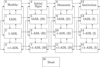
3.1. In this section we set out our model of old age that will form the basis of our LTC models in sections 4 and 5. We start with a continuous-time Markov model of old age as illustrated in Figure 1 and parameterise the transition intensities between states.
A Markov model of functional ability and cognitive function. The arrows to the Dead state are omitted but may be entered from any state

3.2. The Markov framework is an essential assumption for our modelling methodology and is very common in actuarial modelling of life histories. Intuitively, the transitions might be expected to contradict such an assumption. However, there is a difficulty in fitting anything more complex as the data required, such as duration of state occupancy and the path taken to the current state, are often unavailable. Macdonald & Pritchard (Reference Macdonald and Pritchard2000) discusses the Markov nature of the mortality of individuals with AD. They justify the Markov property by citing studies that have found no association between duration of AD and increased mortality (Barclay et al., Reference Barclay, Zemcov, Blass and Sansone1985; Diesfeldt et al., Reference Diesfeldt, Houte and Moerkens1986; Sayetta, Reference Sayetta1986; Walsh et al., Reference Walsh, Welch and Larson1990; Burns et al., Reference Burns, Lewis, Jacoby and Levy1991; Bracco et al., Reference Bracco, Gallato, Grigoletto, Lippi, Lepore, Bino, Lazzaro, Carella, Piccolo, Pozzilli, Giometto and Amaducci1994; Heyman et al., Reference Heyman, Peterson, Fillenbaum and Pieper1996).
3.3. In the absence of data to provide a more suitable model, and for mathematical convenience, we assume all state transitions depend only on the current state, i.e., are Markov.
3.4. For each state ik, we call i its cognitive ability type (the progress of dementia) and k its functional ability type (the number of IADL or ADLs). Changes in cognitive ability type are assumed to be independent of functional ability type. Similarly, changes in functional ability type are assumed to be independent of cognitive ability type. To express this mathematically, we have  $$\mu _{{x{\plus}t}}^{{ik,il}} =\mu _{{x{\plus}t}}^{{jk,jl}} $$
and
 $$\mu _{{x{\plus}t}}^{{ik,jk}} =\mu _{{x{\plus}t}}^{{il,jl}} $$
.
3.5. Inclusion of recoveries adds complexity to the model. However, as mentioned above, Pritchard (Reference Pritchard2006) found that excluding recoveries results in overstating the cost of benefits. For this reason, in our model it is possible to recover from functional disabilities.
3.6. Notation
3.6.1. We introduce the notation that will be used in this section:
(a). As introduced above (and included here for ease of reference),
 $$\mu _{{x{\plus}t}}^{{ik,jl}} $$
is the transition intensity from state ik to state jl at age x+t.
(b). In the case dementia, where genotype-specific intensities are necessary, denote the transition intensity from state ik to state jl at age x+t, for a life with genotype g by
$$\mu _{{x{\plus}t,g}}^{{ik,jl}} $$
.(c). The relative risk of AD caused by APOE genotype g at age x is denoted by, ρ x,g.
(d). Let
$$\hat{\mu }_{{x{\plus}t}}^{i} $$
be the ungraduated force of mortality at age x+t from state 0i estimated by Akodu (Reference Akodu2007).(e). The graduated relative risk of mortality caused by functional disability type i, relative to lives with no ADLs, is denoted by ρ i; while ungraduated for lives aged x is denoted by
$$\hat{\rho }_{{x,i}} $$
.(f). In common with standard actuarial notation, q x+t and p x+t are the 1-year probabilities of death and survival, respectively, for a life aged x+t. After applying mortality improvements, these become
$$q'_{{x,t}} $$
and
$$p'_{{x,t}} $$
, respectively.(g). The factor by which to reduce the 1-year probability of death, t years after the date of the underlying mortality table for a life who was aged x at t=0 is denoted by RFx+t,t,y. The associated reduction factor applicable to
$$\mu _{{x{\plus}t}}^{{00,4}} $$
is denoted by
$\upsilon _{{x,t}} $
.(h). The set of all states in our final Markov model of health is denoted by
${\cal S}$
.


3.7. Functional Ability
3.7.1. Functional ability transition intensities are taken to be those derived by Akodu (Reference Akodu2007), who fitted functions to using the penalised least squares method of Pritchard (Reference Pritchard2006). This is the only study that calculates age-dependent incidence of functional ability for a UK population. It is based on a large body of data (13,004 lives in the first phase of a two phase, longitudinal study) and is fitted with a Markov model, consistent with our assumptions.
3.8. Mortality Without Dementia
3.8.1. We next parameterise the mortality for lives who have not developed dementia (i.e. from state 0j). We observe in Akodu (Reference Akodu2007) that, apart from lives with 1-ADL, the mortality rates experienced by lives in functionally disabled states are significantly higher than the point estimates for lives with no ADLs. Therefore, we will need to fit mortality dependent on functional ability. For simplicity we will use a relative risk approach, where we have some base mortality rate applicable to lives who have no functional disability and apply some factor to calculate mortality for lives with a functional disability.
3.8.2. For a level of consistency with Macdonald & Pritchard (Reference Macdonald and Pritchard2001), we choose as our base mortality rate for lives with no cognitive disability, the Continuous Mortality Investigation’s (CMI) (2009) AMC00 and AFC00 assured lives mortality rates for male and female lives, respectively (the previous study used CMI’s (1990) AM80 and AF80, previous versions of assured mortality). They were calculated from the experience of subscribing UK insurance companies over the period 1999–2002, and they apply to a life attaining age x on the 1 July 2000.
3.8.3. We calculate the relative risks of death using data from Akodu (Reference Akodu2007). The ungraduated relative risk of mortality, relative to lives with no ADLs,  $$\hat{\rho }_{{x,i}} $$
, is calculated as
 $$\hat{\rho }_{{x,i}} ={{\hat{\mu }_{x}^{i} } \over {\hat{\mu }_{x}^{0} }}$$
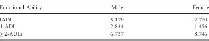
For simplicity, we fit a constant relative risk of mortality for functional disability type i, as the weighted average over all ages, where the weight for age x is  $$1/{\rm Var}(\hat{\mu }_{x}^{i} )$$
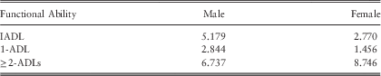
. These are shown in Table 1. The mortality rate for state ij is given by
 $$\mu _{{x{\plus}t}}^{{ij,4}} =\rho _{i} \mu _{{x{\plus}t}}^{{0j,4}} $$
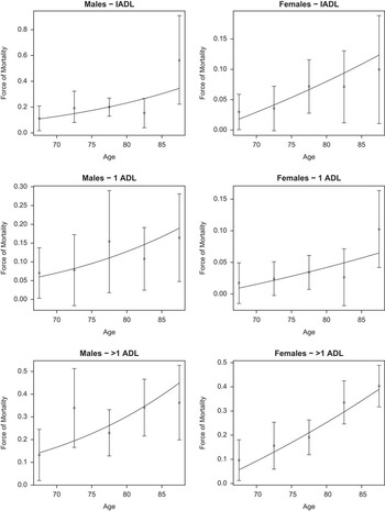
3.8.4. To check consistency with the CFAS data, we apply these relative risks, relative to Akodu’s (Reference Akodu2007) fitted force of mortality for lives with no ADLs, in Figure 2. For each level of functional disability, the force of mortality is within 95% confidence intervals at every age, hence there would be no evidence against our constant relative risks.
Forces of mortality in a relative risk model. Point estimates and confidence intervals are from Akodu (Reference Akodu2007)

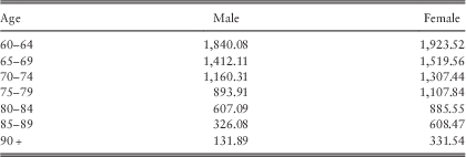
Relative Risk of Mortality According to Functional Ability Type, Relative to a Life With No ADLs, for Males and Females
ADL, activity of daily living; IADL, instrumental activity of daily living.
3.9. Mortality Improvements
3.9.1. Recent years have shown substantial improvements in mortality (Office for National Statistics, 2012b). To project the mortality improvements, we use CMI’s (2011) mortality projections model, which combines cohort effects and age effects of mortality improvement.
3.9.2. The method used by CMI (2011) to apply these improvement rates to a mortality table is to first calculate a set of base reduction factors, using all of the available observed data, i.e., from 1 January 1990. From this base reduction factor, they rebase it to the date of the mortality table being used. The base reduction factors,  $${\rm RF}_{{x,t}}^{{\asterisk}} $$
are calculated at integer age x, and time since the date of our mortality table t as for non-integer x and t, we calculate RFx,t,y using geometric interpolation: first on age, and second on time, as
 $$\eqalignno{ {\rm RF}_{{x,t,y}} =&\,\left( {{\rm RF}_{{\left\lfloor x \right\rfloor ,\left\lfloor t \right\rfloor ,y}} ^{{^{{1{\minus}\left( {x{\minus}\left\lfloor x \right\rfloor } \right)}} }} {\rm RF}_{{\left\lfloor x \right\rfloor {\plus}1,\left\lfloor t \right\rfloor ,y}} ^{{x{\minus}\left\lfloor x \right\rfloor }} } \right)^{{1{\minus}\left( {t{\minus}\left\lfloor t \right\rfloor } \right)}} \cr & {\times}\left( {{\rm RF}_{{1{\plus}\left\lfloor x \right\rfloor ,1{\plus}\left\lfloor t \right\rfloor ,y}} ^{{^{{1{\minus}\left( {x{\minus}\left\lfloor x \right\rfloor } \right)}} }} {\rm RF}_{{2{\plus}\left\lfloor x \right\rfloor ,1{\plus}\left\lfloor t \right\rfloor ,y}} ^{{^{{x{\minus}\left\lfloor x \right\rfloor }} }} } \right)^{{\left( {t{\minus}\left\lfloor t \right\rfloor } \right)}} $$
3.9.3. This produces factors to reduce q x, the 1-year probability of death, at integer ages and times:  $$q'_{{x,t}} ={\rm RF}_{{x{\plus}t,t,y}} \:q_{{x{\plus}t}} $$
and
 $$p'_{{x,t}} =1{\minus}q'_{{x,t}} $$
. However, we use the force of mortality
 $$\mu _{{x{\plus}t}}^{{00,4}} $$
so we need to calculate a consistent factor to improve the force of mortality.
3.9.4. Now, RFx,0,y=1, i.e.,  $$q_{x} =q'_{{x,0}} $$
, therefore
 $$\mathop{\int}\nolimits_0^1 \mu _{{x{\plus}t}}^{{00,4}} dt=\mathop{\int}\nolimits_0^1 \upsilon _{{x,t}} \mu _{{x{\plus}t}}^{{00,4}} dt$$
so
 $$\upsilon _{{x,t}} {\rm =1}$$
for 0≤t≤1. For t≥1 we have
 $$\matrix{ {_{h} p'_{{x,t}} =\displaystyle{{_{{1{\plus}h}} p'_{{x,t{\minus}1}} } \over {p'_{{x,t{\minus}1}} }}} \cr {\exp \left( {{\minus}\mathop{\int}\limits_0^h {\upsilon _{{x,t{\plus}s}} \,\mu _{{x{\plus}t{\plus}s}}^{{00,4}} ds} } \right)=\displaystyle{{p'_{{x,t{\plus}h{\minus}1}} \exp \left( {{\minus}\mathop{\int}\limits_0^h {\upsilon _{{x,t{\minus}1{\plus}s}} \,\mu _{{x{\plus}t{\minus}1{\plus}s}}^{{00,4}} ds} } \right)} \over {p'_{{x,t{\minus}1}} }}} \cr {\upsilon _{{x,t{\plus}h}} =\displaystyle{{{\minus}\displaystyle{{{d \over {dh}}p'_{{x,t{\plus}h{\minus}1}} } \over {p'_{{x,t{\plus}h{\minus}1}} }}{\plus}\upsilon _{{x,t{\minus}1{\plus}h}} \,\mu _{{x{\plus}t{\minus}1{\plus}h}}^{{00,4}} } \over {\mu _{{x{\plus}t{\plus}h}}^{{00,4}} }}} \cr } $$
For t≥1, to solve equation (4), we approximate the derivative  $${d \over {dh}}p'_{{x,t{\plus}h{\minus}1}} $$
numerically with a central difference method:
 $${d \over {dh}}p'_{{x,t{\plus}h{\minus}1}} \,\approx\,{{p'_{{x,t{\plus}2h{\minus}1}} {\minus}p'_{{x,t{\minus}1}} } \over {2h}}$$
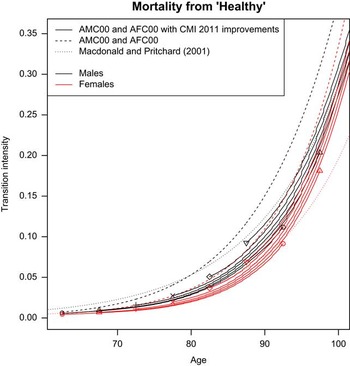
3.9.5. The mortality intensities from the healthy state are for lives attaining age x on 1 July 2000, while our modelling date is some 12.5 years later, on 1 January 2013. The results of this mortality improvement applied to lives in Healthy are shown in Figure 3. The force of mortality used by Macdonald & Pritchard (Reference Macdonald and Pritchard2001) is higher than what we use, particularly for males; while at the oldest ages theirs is lower, particularly for females. This is driven by the pattern of mortality improvements: as we have discussed, there are birth year and age effects on mortality improvement, whereas Macdonald & Pritchard (Reference Macdonald and Pritchard2001) assumed an average improvement factor applicable to all lives.
Force of mortality from the “Healthy” state with and without mortality improvements. Improved mortality shown from 2013 with points representing the start and end points of a 30-year period for lives aged 62.5,67.5, …, 87.5 in 2013

3.10. Genetics of AD
3.10.1. In this section we describe the impact of the APOE gene in AD onset and parameterise a genetic component of the disease into our model.
3.10.2. The major genetic risk factor for AD is the APOE gene (Coon et al., Reference Coon, Myers, Craig, Webster, Pearson, Lince, Zismann, Beach, Leung, Bryden, Halperin, Marlowe, Kaleem, Walker, Ravid, Heward, Rogers, Papassotiropoulos, Reiman, Hardy and Stephan2007), which codes for a protein that transports lipids around the circulatory system. There are at least three allele variants, the most common of which are named ε2, ε3 and ε4. This leads to possible six genotypes: ε2ε2, ε2ε3, ε2ε4, ε3ε3, ε3ε4 and ε4ε4. Relative to ε3, ε4 makes a life more susceptible to developing AD, while ε2 reduces susceptibility. However, the processes that cause these differences in susceptibility are yet to be established (Huang & Mucke, Reference Huang and Mucke2012).
3.10.3. It is possible to test which variants are present in a life’s genome, indeed this is among the genes tested by companies offering genetic tests to individuals such as 23andMe.Footnote 1 However, it is unlikely to be used predictively by doctors in relation to AD, as there is currently no preventative treatment available and the test results might create undue stress to the life. Low et al. (Reference Low, Yap and Brodaty2010) found there was insufficient evidence to recommend testing to aid in prescribing risk reduction methods for dementia, while Farrer et al. (Reference Farrer, Brin, Goate, Kennedy, Mayeux, Myers, Reilly and Risch1995) recommends against its use for the reason that APOE alone is insufficient in accurately predicting age of onset.
3.10.4. APOE was considered to be a susceptibility gene for coronary heart disease (CHD) (Song et al., Reference Song, Stampfer and Liu2004). However, there is debate as to the validity of the link. In a large study, which controlled for the variety of known cardiovascular risk factors, Ward et al. (Reference Ward, Mitrou, Bowman, Luben, Wareham, Tee Khaw and Bingham2009) found no association between APOE and CHD. A recent study by Kofler et al. (Reference Kofler, Miles, Curtis, Armah, Tricon, Grew, Napper, Farrell, Lietz, Packard, Caslake, Mathers, Williams, Calder and Minihane2012) analysed the interaction of APOE with body mass index, age and sex and concluded that the risk of developing CHD owing to APOE genotype was “unlikely to be homogeneous”. Nonetheless, while the link and risk factors of particular genotypes for CHD are still being studied, it remains plausible that testing for APOE genotype might one day be useful in devising treatment for diseases other than AD. This broadens the possibility that individuals could learn of their genetic susceptibility to AD even if that was not the intention. We therefore incorporate APOE genotypes into our model of health, which will allow us to use this as a source of adverse selection.
3.10.5. Denote the set of APOE genotypes by  ${\cal G}$
. Owing to the rarity of ε2ε2 and consistent with Macdonald & Pritchard (Reference Macdonald and Pritchard2000, Reference Macdonald and Pritchard2001), we group these together with ε2ε3 and consider them indistinguishable. Therefore, we have
 ${\cal G}{\rm =}\left\{ {{\varepsilon}2{\varepsilon}2,\,{\varepsilon}2{\varepsilon}4,\,{\varepsilon}3{\varepsilon}3,\,{\varepsilon}3{\varepsilon}4,\,{\varepsilon}4{\varepsilon}4} \right\}$
.
3.10.6. We use the fitted relative risks of Macdonald & Pritchard (Reference Macdonald and Pritchard2001) because these are still the most useful available.
3.11. Onset of Dementias
3.11.1. In this section we will fit transition intensities for non-AD and AD, respectively, in order to apply gene-specific relative risks only to AD onset. Our model does not have separate states for the different types of dementia, so we calculate dementia onset as the total of these two components.
3.11.2. Launer et al. (Reference Launer, Andersen, Dewey, Letenneur, Ott, Amaducci, Brayne, Copeland, Dartigues, Kragh-Sorensen, Lobo, Martinez-Lage, Stijnen and Hofman1999) pooled four population-based prospective studies of onset rates and risk factors for dementia as a whole and AD in particular. These were all part of the European Studies of Dementia (EURODEM) Launer, Reference Launer1992. We choose Launer et al. (Reference Launer, Andersen, Dewey, Letenneur, Ott, Amaducci, Brayne, Copeland, Dartigues, Kragh-Sorensen, Lobo, Martinez-Lage, Stijnen and Hofman1999) because they reported exposures and number of diagnoses for AD and dementia in 5-year age groups, allowing maximum likelihood estimation of model parameters. Moreover, the largest contribution to EURODEM, by size of cohort, came from the UK study (Copeland et al., Reference Copeland, McCracken, Dewey, Wilson, Doran, Gilmore, Scott and Larkin1999).
3.11.3. The genetic relative risks for AD in section 3.10 are sex specific and applied to the aggregate onset rate so we fit the aggregate onset rate here. However, we note that although results separated by gender were not published, sex was found to be a significant risk factor for AD by Launer et al. (Reference Launer, Andersen, Dewey, Letenneur, Ott, Amaducci, Brayne, Copeland, Dartigues, Kragh-Sorensen, Lobo, Martinez-Lage, Stijnen and Hofman1999), with female rates 54% higher than male rates, but no significant difference was observed for non-AD dementia.
3.11.4. Denote the population average onset rate of AD at age x by  $$\mu _{x}^{{{\rm AD}}} $$
and the onset rate of non-AD dementia by
 $$\mu _{x}^{{{\rm NAD}}} $$
. Owing to the small size of the data set, we seek the simplest relationship between non-AD dementia and AD dementia transition intensities such that
 $$\mu _{x}^{{{\rm NAD}}} /\mu _{x}^{{{\rm AD}}} =\kappa $$
for some constant κ.
3.11.5. Using the method of maximum likelihood, we fit the Gompertz–Makeham (GM) family of models to  $$\mu _{x}^{{{\rm AD}}} $$
and
 $$\mu _{x}^{{{\rm NAD}}} $$
. With
 $$\mu _{x}^{{{\rm NAD}}} =\kappa \:\mu _{x}^{{{\rm AD}}} $$
, the likelihood function to be maximised is
 $$L\propto{{\left( {e_{x}^{{{\rm NAD}}} \:\kappa \:\mu _{x}^{{{\rm AD}}} } \right)^{{d_{x}^{{{\rm NAD}}} }} } \over {d_{x}^{{{\rm NAD}}} \,!\,}}{{\left( {e_{x}^{{{\rm AD}}} \:\mu _{x}^{{{\rm AD}}} } \right)^{{d_{x}^{{{\rm AD}}} }} } \over {d_{x}^{{{\rm AD}}} \,!\,}}\exp \left( {{\minus}e_{x}^{{{\rm NAD}}} \:\kappa \:\mu _{x}^{{{\rm AD}}} {\minus}e_{x}^{{{\rm AD}}} \:\mu _{x}^{{{\rm AD}}} } \right)$$
Detailed results of this fitting process can be found in Adams (Reference Adams2013).
3.11.6. We find that Akaike’s information criterion is minimised with a GM(0,3) model:
 $$\mu _{x}^{{{\rm NAD}}} =0.5\mu _{x}^{{{\rm AD}}} =0.5\,\exp \left( {{\minus}40.9847{\plus}0.762795x{\minus}0.00379x^{2} } \right)$$
3.11.7. The overall dementia intensity is therefore
 $$\mu _{{x,g}}^{{0i,1i}} =\left( {0.5{\plus}\varrho _{{x,g}} } \right){\rm exp}\left( {{\minus}40.9847{\rm {\plus}}0.762795x{\minus}0.00379x^{2} } \right)$$
3.11.8. The shape of the chosen model has decreasing intensities among the oldest old (>100 years old). There is very little data available for such ages and as any LTC claim would be short (owing to the very high mortality at such ages) there would be little distortion of adverse selection costs, we proceed with the transition intensities as they have been fitted.
3.12. Post-Dementia Mortality
3.12.1. In this section we parameterise the force of mortality for lives with dementia, and lives who have been put into a nursing care facility because of dementia. We assume the same relative risks owing to functional ability, as derived in section 3.8, applies after diagnosis of dementia and that the transition intensities fitted here apply to lives with no ADLs.
3.12.2. Several studies have been performed to identify any difference in the survivorship of Alzheimer’s-type dementia and that of vascular dementia. Burns (Reference Burns1993) summarises the findings of 12 of these studies. While three of them (including the largest study) found vascular dementia to have poorer survivorship, the majority could not find any significant difference in the prognosis between the two forms of dementia. There is also a possibility of heterogeneity in the classification: as AD can only be confirmed through autopsy, there may have been cases of mis-diagnosis of dementia type. As vascular dementia is the most common of the non-AD dementias, we use this as a proxy for all non-AD types and assume the mortality of lives with any form of dementia as independent of the type of dementia.
3.12.3. Colgan (Reference Colgan2006) found the forces of mortality for lives with AD and for those with AD in an institution using data from CERAD. CERAD was a case-control study of sufferers of AD in the United States, which aimed to observe the progression of the disease, including the progression into a nursing home, through annual examinations. Confirmation of diagnoses through autopsy was performed where possible. The analysis covers the period 1986–1995, so we assume the rates are effective for a life attaining age x on the 1 January 1990.
3.12.4. Macdonald & Pritchard (Reference Macdonald and Pritchard2000) fitted mortality rates to a very small data set, which limited the number of parameters they could fit and chose simple adjustments to their healthy mortality. We use Colgan’s (Reference Colgan2006) work as it uses a larger data set and is based on the raw data rather than summary statistics (which Macdonald & Pritchard, Reference Macdonald and Pritchard2000 used).
3.12.5. The force of mortality after diagnosis but before institutionalisation for males was found to be significantly different to females, so sex-specific rates were calculated. For males this was
 $$\mu _{x}^{{10,4}} =\exp \left( {{\minus}8.17{\plus}0.071x} \right)$$
and for females it was
 $$\mu _{x}^{{10,4}} =0.029{\plus}\exp \left( {{\minus}22.014{\plus}0.221x} \right)$$
3.12.6. The force of mortality after institutionalisation for males was also found to be significantly different to females, so sex-specific rates were calculated. For males it was
 $$\mu _{x}^{{20,4}} =\exp \left( {{\minus}5.13{\plus}0.052x} \right)$$
and for females it was
 $$\mu _{x}^{{20,4}} =0.105{\plus}\exp \left( {{\minus}16.220{\plus}0.166x} \right)$$
We apply the same mortality improvements model to each of these, as we used for non-demented mortality (see section 3.9). The results of this are shown in Figures 4a and 5b. For comparison, also shown are the forces of mortality used by Macdonald & Pritchard (Reference Macdonald and Pritchard2001).
Force of mortality with and without Continuous Mortality Investigation (CMI) improvements

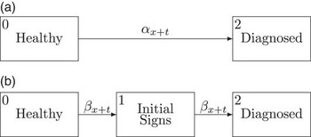
(a) Model A: a two-state model of the onset of dementia. (b) Model B: a three-state model of the onset of dementia

3.12.7. As Colgan (Reference Colgan2006) noted, Macdonald & Pritchard’s (Reference Macdonald and Pritchard2000) mortality intensities before institutionalisation are much lower. The results, which the latter used, suggested lighter mortality than that of healthy lives, which they justified as being because of informal care that sufferers would be receiving while their symptoms progressed.
3.12.8. For the post-institutionalisation mortality, Colgan (Reference Colgan2006) is initially lighter and higher at older ages. Colgan (Reference Colgan2006) suggested it was because of Macdonald & Pritchard’s (Reference Macdonald and Pritchard2000) limitation of fitting as a simple function of their baseline mortality, thereby being restricted in the shape.
3.13. Institutionalisation After Dementia
3.13.1. In this section we parameterise the progression after being diagnosed with dementia to the state where they require care in an institution.
3.13.2. Ballard et al. (Reference Ballard, O’Brien, Barber, Neill and McKeith2001) found that the major causes of dementia (AD, vascular dementia and dementia with Lewy bodies) had similar progression. We therefore assume that the cognitive decline is independent of the dementia type, i.e., an individual who is diagnosed with dementia will reach a stage where they require nursing care at the same rate, regardless of what caused the dementia to occur.
3.13.3. Colgan (Reference Colgan2006) fitted a model for transition intensities into an institution after diagnosis with AD to CERAD data. He found no significant difference between males and females so fitted in aggregate. Under our assumption of equal progression, this is assumed to apply to any dementia, hence
 $$\mu _{x}^{{10,20}} =\exp ({\minus}2.92{\plus}0.016x)$$
3.14. Undiagnosed Dementia
3.14.1. As dementia is progressive, it may be noticeable to the life or their family members before a clinical diagnosis. Without details of the disease in medical records, the insurer’s ability to detect it in propositions is limited to its own underwriting mechanisms (e.g. asking the customer to remember words at the start of a telephone underwriting session and testing their ability to remember these words at the end of the call) and thereby giving rise to possible information asymmetry and adverse selection in LTC. Introducing to our model (as shown in Figure 6), an intermediate stage of cognitive decline where the individual shows some of the signs, e.g., memory degrading at an increased rate, will allow us to use a higher rate of insurance purchase from those lives who have noticed this greater need for long-term care and assess the cost of this source of adverse selection. We assume the dementia has not yet reached a stage where the insurer’s underwriting tools are able to detect the dementia.
A Markov model of functional ability and cognitive function with a stage in cognitive decline where the initial signs of dementia have not been diagnosed but are visible to the individual. The arrows to the Dead state are omitted but may be entered from any state

3.14.2. We now need to parameterise the transition intensities between the stages of cognitive function. Choosing the Initial Signs state such that the rate of entry to the state is equal to the rate of exit simplifies the parameterisation to calculating one transition intensity. This is purely a modelling assumption, which acts as a means of introducing the possibility of such a state into the model. In reality the rates in and out of this state could differ – particularly as having suspicions might be expected to cause the life to go to the doctor for diagnosis. Moreover, our Markov assumption may be expected to break down.
3.14.3. By further assuming that mortality is unaffected at this early stage of dementia, all transition intensities are independent of whether the life is healthy or has the initial signs of dementia. This allows us to reduce the parameterisation to models with only the cognitive function transitions without any further loss of generality:
(a). Model A – consider a two-state model used to represent a life by whether they have been medically diagnosed (this is shown in Figure 5a).
(b). Model B – if we insert a state representing when the life has noticed the initial signs of dementia but before being medically diagnosed, we will get the three-state model depicted in Figure 5b.
3.14.4. Let α t be transition intensity between Healthy and Diagnosed. This can be observed and estimated from prospective studies. However, our intermediate Initial Signs (1) state is at some arbitrary stage between Diagnosis (2) and Healthy (0) and as such, the transition intensities are unavailable. Let β t be this unknown transition intensity between Healthy and Initial Signs, and between Initial Signs and Diagnosed. In terms of our models, which include functional disability,  $$\mu _{{x,g}}^{{0i,1i}} =\alpha _{t} $$
and
 $$\mu _{{x,g}}^{{0,4}} =\mu _{{x,g}}^{{4,8}} =\mu _{{x,g}}^{{1,5}} =\,\ldots\,\:\mu _{{x,g}}^{{7,11}} =\beta _{t} $$
.
3.14.5. To ensure consistency between both models, we require the probabilities of being diagnosed under models A and B to be equal. Denote by  $$_{t} A_{x}^{{ij}} $$
, the probability of being in state j at age x+t conditional on being in state i at age x under model A and similarly for model B,
 $$_{t} B_{x}^{{ij}} $$
. If we assume no lives have developed the initial signs at age x, our equivalence requirement can be represented by
 $$_{t} A_{x}^{{02}} =_{t} B_{x}^{{02}} $$
or alternatively
 $$_{t} A_{x}^{{00}} =\,_{t}\!\!B_{x}^{{00}} {\plus}_{t} B_{x}^{{01}} $$
3.14.6. Clearly,  $$_{t} B_{x}^{{00}} =\exp \left( {{\minus}\mathop{\int}\nolimits_0^t \beta _{{x{\plus}s}} \:ds} \right)$$
and similarly
 $$_{t} A_{x}^{{00}} =\exp \left( {{\minus}\mathop{\int}\nolimits_0^t \alpha _{{x{\plus}s}} \:ds} \right)$$
. For
 $$_{t} B_{x}^{{01}} $$
we have
 $$\eqalignno{ _{t} B_{x}^{{01}} & =\mathop{\int}\nolimits_0^t _{_s} B_{x}^{{00}} \beta _{{x{\plus}s}} \:_{{t{\minus}_s}} B_{{x{\plus}s}}^{{11}} \:ds \cr & =\,_{t}\!\!B_{x}^{{00}} \mathop{\int}\nolimits_0^t \beta _{{x{\plus}s}} \:ds $$
3.14.7. Inserting equation (15) into equation (14) yields a differential equation for β t in terms of α t:
 $$\beta _{{x{\plus}t}} =\alpha _{{x{\plus}t}} \left( {{{1{\plus}\mathop{\int}\nolimits_0^t \beta _{{x{\plus}s}} \:ds} \over {\mathop{\int}\nolimits_0^t \beta _{{x{\plus}s}} \:ds}}} \right)$$
3.14.8. To avoid β x+t exploding to infinity at t=0, for some small time step h, we assume β x=β x+s, for s∈[0,h]. This assumption allows us to calculate β x as
 $$\eqalignno{ \beta _{x} =\beta _{{x{\plus}h}} & =\alpha _{{x{\plus}h}} \left( {{{1{\plus}\beta _{{x{\plus}h}} h} \over {\beta _{{x{\plus}h}} h}}} \right) \cr & ={{\alpha _{{x{\plus}h}} h\,\pm\,\sqrt {\alpha _{{x{\plus}h}}^{2} h^{2} {\plus}4\alpha _{{x{\plus}h}} h} } \over {2h}} $$
4. Simulating LTC Payments
4.1. In this section we describe how simulation can be used to estimate the expected present values of benefits and premiums in a LTC contract.
4.2. Notation
4.2.1. We first define the notation introduced in this section, which will be used in later sections.
a. The force of interest and force of inflation are assumed constant at rates δ per annum and v per annum, respectively.
b. The set of periods that a policy may go through is denoted by
${\cal P}{\rm =}\left\{ {P,\,C,\,D} \right\}$
, and consists of P – after inception but before any claim; C – after a claim on a functional disability but before dementia; D – after the first claim involving dementia.c. For a life aged x at the simulation start date, of sex
$\varsigma $
, with genotype g and insured at time t, from health state j.d. The smoothed probability that this life is in period
$\rho \in {\cal P}$
at the start of calendar year c is denoted by
$$_{c} p_{{x,\varsigma ,g,t}}^{{j,\rho }} $$
.e. Given this life is in period ρ, the smoothed average present value of future benefits and premium income are denoted by
$$A_{{x,\varsigma ,g,t:c}}^{{j,\rho }} $$
and
$$a_{{x,\varsigma ,g,t:c}}^{{j,\rho }} $$
, respectively.


4.3. Reason for Simulation Approach
4.3.1. The model of health depicted in Figure 6 is Markov – transition intensities depend on the state currently occupied, not the path to get there. However, LTC payments could be capped by the insurer with a limit on annual payouts or some total sum assured, or the government could limit the liability faced by the individual before state support is paid (a policy currently under discussion in the United Kingdom, which we discuss further in section 6). In cases such as these, the cashflow at any point in time depends not only on the current health status, but on the entire history of health statuses.
4.3.2. This disjoint nature between the cashflows and current health status creates a difficulty in calculating the expected present value of benefits for the purpose of setting premiums. Consider a contract with all the limits as described above, bought by a life aged x, when in state i:
a. The insurer limits total of payments over the lifetime of the policy to sum assured, s, and the benefits payable within a calendar year to, a.
b. The government pays for care costs once the individual’s care liability (which may be paid by the insurer) has surpassed, g.
c. “Hotel” costs (accommodation cost in a care home) are excluded from the government cap but covered by the insurer, up to its own benefit limits.
d. The care and hotel costs for state j, amount to c j and h j, respectively.
e. All costs and caps increase over time at the same constant force of inflation, denoted by v. All benefit payments and caps are compared at the same purchasing power.
Let  $$_{t} I_{x}^{j} $$
be an indicator random variable such that
 $$_{t} I_{x}^{j} {\rm =}\left\{ {\matrix{ 1 & {{\rm if}\ x\ {\rm is}\ {\rm in}\ j\ {\rm at}\ {\rm age}\ x{\plus}t} \cr 0 & {{\rm otherwise}} \cr } } \right.$$
Let I(ƒ) be another indicator function such that
 $$I\left( f \right){\rm =}\left\{ {\matrix{ 1 & {{\rm if}\,f\,\gt\, 0} \cr 0 & {{\rm otherwise}} \cr } } \right.$$
We denote the random variable representing the care cost if x is in state j at time t, as a continuously payable annual rate, by  $$_{t} C_{x}^{j} $$
and calculate it as
 $$_{t} C_{x}^{j} =c_{j} e^{{\nu t}} I\left( {g{\minus}\mathop{\sum}\limits_l \mathop{\int}\nolimits_{{\minus}x}^t {}_{r}I_{x}^{l} \:_{r} C_{x}^{l} e^{{{\minus}\nu r}} \:dr} \right)$$
We further denote the random variable representing the insurance benefit payment if x is in state j at time t, as a continuously payable annual rate, by  $$_{t} B_{x}^{j} $$
and calculate it as
 $$\eqalignno{ _{t} B_{x}^{j} =\left( {_{t} C_{x}^{j} {\plus}h_{j} e^{{\nu t}} } \right) \quad& I\,\left( {s{\minus}\mathop{\sum}\limits_l \mathop{\int}\nolimits_0^t _{_r} I_{x}^{l} \:_{_r} B_{x}^{l} e^{{{\minus}\nu r}} \:dr} \right) \cr & {\times}I\left( {a{\minus}\mathop{\sum}\limits_l \mathop{\int}\nolimits_{\left\lfloor t \right\rfloor }^t _{_r} I_{x}^{l} \:_{_r} B_{x}^{l} e^{{{\minus}\nu r}} \:dr} \right) $$
4.3.3. The expected present value of benefits paid to x can then be calculated as
 $$E\,\left( {{\rm PV}\,{\rm benefits}\,{\rm payable}\,{\rm to}\,x} \right)=E\left( {\mathop{\sum}\limits_j \mathop{\int}\nolimits_0^\infty {}_{r}B_{x}^{j} \:_{_r} I_{x}^{j} e^{{{\minus}\delta r}} \:dr} \right)$$
4.3.4. Equation (22) involves a complicated system of integration, which is simplest to solve approximately using simulation. We perform simulations of future lifetimes and the consequent LTC benefit cashflows that occur (by solving equations (20) and (21)). Equation (22) can then be found by taking the average of the discounted values of our simulated benefit cashflows. If we assume that no care liability has been faced before purchasing insurance, we avoid the complication of setting premium rates for a varying degree of potential benefit sizes (as limited by the government cap) and simplify our pricing problem to simulating from the point of insurance purchase.
4.4. Simulation Method
4.4.1. To simulate life histories, represented by transitions between states in our health model, we first find the time of a transition. By conditioning on the transition occurring at this time, we then find the state the life moves to. Denote the random variables representing the time of the ith transition by T i and S i as the state a life is in after the ith transition. Further, denote the value taken by them as t i and s i, respectively. We assume a life aged x at the start of the simulation is in state s 0 at time t 0=t. For a life in state s i−1 at time t i−1, we simulate the next transition time using the inverse transform method (Devroye, Reference Devroye1986) solving  $$F_{{T_{i} }} (t_{i} )=u$$
where u is an observation from the Uniform [0,1] distribution and
 $$F_{{T_{i} }} (t_{i} )=1{\minus}\exp \left( {{\minus}\mathop{\int}\nolimits_{t_{{i{\minus}1}} }^{t_{i} } \mathop{\sum}\limits_{j\in {\cal S}} \mu _{{x{\plus}u}}^{{s_{{i{\minus}1}} ,j}} du} \right)$$
for t i. These integrals are solved using Simpson’s rule with a step size of 2−11 and our simulation period is 30 years to capture most of a life’s future lifetime.
4.4.2. Given a life makes the ith transition at time t i, the probability that the movement was to state j is
 $$P(S_{i} =s_{i} \,\mid\,T_{i} =t_{i} )={{\mu _{{x{\plus}t_{i} }}^{{s_{{_{{i{\minus}1}} }} ,s_{i} }} } \over {\mathop{\sum}\limits_{j\in {\cal S}} \mu _{{x{\plus}t_{i} }}^{{s_{{_{{i{\minus}1}} }} ,j}} }}$$
Define the conditional cumulative distribution function as
 $$F_{{S_{i} \,\mid\,T_{i} =t_{i} }} (s_{i} )=P(S_{i} \leq s_{i} \,\mid\,T_{i} =t_{i} )={{\mathop{\sum}\limits_{j=0}^{s_{i} } \mu _{{x{\plus}t_{i} }}^{{s_{{i{\minus}1}} ,j}} } \over {\mathop{\sum}\limits_{j\in {\cal S}} \mu _{{x{\plus}t_{i} }}^{{s_{{i{\minus}1}} ,j}} }}$$
We simulate the jump at time t i by applying the inverse transform method on  $$F_{{S_{i} \,\mid\,T_{i} =t_{i} }} (s_{i} )=v$$
, where v is an observation from the Uniform [0,1] distribution, solving for s i.
4.4.3. With knowledge of the future lifetime of our simulated life, we can calculate the present value payments in respect of a LTC contract bought at time t 0. By averaging over a large number of simulations, we calculate an estimate of equation (22). To allow a product design with regular premiums, we also estimate the expected present value of an annuity in premium paying states, which we refer to as the premium annuity. The premium annuity and benefit payments are increased at the same force of inflation, v per annum. As in our above example, all benefit payments and caps are compared at the same purchasing power.
4.4.4. We assume that a life cannot buy insurance if it would put them into a claim immediately. In addition, as we are primarily concerned with the potential cost of adverse selection, we do not model the purchase of insurance after dementia has been diagnosed – this is observable to an insurer so we assume they can underwrite them appropriately. We call the set of remaining states insurable.
4.4.5. As we simulate from the point of insurance purchase, we require the exposed process values from each time step at which insurance can be purchased, which we refer to as purchase time steps. Owing to the computing time required, we restrict our purchase time steps to the 30-year period in steps of 0.015625 years. Simulations are performed for 50,000 lives at each purchase time step, for males and females of each APOE genotype for each insurable state. Thus, we perform 50,000×2×5×6=3,000,000 simulations at each purchase time step.
4.5. Information Gained by the Insurer
4.5.1. Integral to adverse selection is the notion of asymmetric information – where the policyholder knows more about their health than the insurer. Over time, the insurer can learn about the mix of business it has on its books, based on its claims experience. By better understanding the mix of lives to whom they have been selling, the insurer will be better placed to estimate the mix of future business and the premiums to charge. This will form the basis for the dynamic premium rates of section 5.4.
4.5.2. From details of claims payouts, an insurer could observe three key events over the lifetime of a policy, which will change their knowledge of the mix of business:
a. Inception – at the point of inception, the insurer has no information on the actual mix of business beyond what is implied in the pricing basis.
b. A claim for functional disability (unrelated to dementia) – the insurer now knows what functional disability state the life is in; transition between states of functional disability is determined only by current functional disability.
c. Claim involving dementia – when the insurer knows the life has dementia (we assume they also learn of functional disability at this point also), everything relevant to its future transitions is now known and no more useful information is gleaned from further claims.
These observations will tell them more about the mix of the policyholders than was known at underwriting and allow them to more accurately value future cashflows in the periods following them:
a. P – after inception but before any claim.
b. C – after the first functional disability claim but before a claim involving dementia.
c. D – after the first claim involving dementia.
The set of these periods can therefore be written as,  $${\cal P}$$
={P,C,D}. We explain further by use of an example: assume some benefit is payable to an insured life while in states {3,7,10,11,12,13,14,15}. Consider life x, who bought his insurance from state 5 at time t 0. The insurer cannot distinguish him from any other life in states {0,1,2,4,5,6}:
a. x reaches state 7 at time t 1, making a claim unrelated to dementia. The insurer now knows he is in either state 3 or state 7 and can improve its modelling in respect of this.
b. x recovers to state 6 at time t 2.
c. x subsequently claims again in state 7 at time t 3. In a large portfolio of business, this does not tell the insurer anything new because x’s transitions between functional disability are being modelled appropriately already based on being in either state 3 or state 7 at time t 1 and the Markov nature of the model (recall that functional ability transitions are assumed to be independent of cognitive function).
d. x develops dementia and claims from state 11 at time t 4. The insurer knows x is in state 11 and updates its model with this information.
e. x’s claim ceases upon movement to state 8 at time t 5.
f. x dies at time t 6.
In this example, period P was from t 0 until t 1; period C was from t 1 until t 4; and period D was from t 4 until the policy ended at t 6.
4.5.3. To model this information development, at the start of each calendar year of our simulations, we calculate the probability that a life, who purchased insurance at time t, is in each period. In addition, we estimate the expected present value of all future benefits and of future income (including those cashflows that will occur within a subsequent period) for lives who are in each of our periods.
4.6. Smoothing
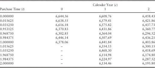
4.6.1. The simulated expected present values and probabilities within each calendar year c are smoothed with respect to insurance purchase time t≤c+1, by fitting cubic splines using the ALGLIB package for C++ (Bochkanov & Bystritsky, Reference Bochkanov and Bystritsky2013). This removes the random noise and gives us a means of estimating the expected present values,  $$A_{{x,\varsigma ,g,t:c}}^{{j,\rho }} $$
and
 $$a_{{x,\varsigma ,g,t:c}}^{{j,\rho }} $$
, and the probability of being in period ρ,
 $$_{c} p_{{x,\varsigma ,g,t}}^{{j,\rho }} $$
, for any insurance purchase date t≤c+1. Splines are fitted to these independently for every combination of initial age, sex, genotype, policy period and the health state which insurance was purchased from.
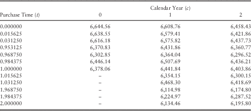
4.6.2. To explain further what smoothing is performed, in Table 2 we present the simulated present values of benefits for males in period P, with genotype ε2ε2, who were aged 62.5 at calendar year 0 and buy insurance at time t from state 0. In each calendar year for which the life has not yet made any claim, all future premium payments are discounted to the start of the year. Purchases at integer times are considered to be in force in the year before to provide a knot for fitting the final section of the year – in the table, when t=1, there is a value for c=0. Smoothing is then performed on each column independently, with respect to t.
Simulated Present Values of Future Benefits for Males in Period P, with Genotype ε2ε2, Aged 62.5 at Calendar Year 0, Buying Insurance from State 0
5. LTC Market
5.1. In this section we set up a model for the market of LTC by adding states our health model of Figure 6, to represent the presence of insurance. To allow us to set higher (or lower) rates of insurance purchase from lives who have received a genetic test (and hence allow this as a source of adverse selection), we also add states representing whether a genetic test has been received. This market model is depicted in Figure 7.
A Markov model of an insurance market for long-term care insurance (LTC) where ι denotes whether the life is insured, and ϑ denotes whether a genetic test has been performed. The arrows to the Dead state are omitted but may be entered from any state

5.2. We name each state by reference to its insured status, its test status, ι∈B, and its health status,  $$i\in {\cal S}$$
, as ιϑi, where B={0,1},
 $$\vartheta {\rm =}\left\{ {\matrix{ 0 & {{\rm if}\,{\rm the}\,{\rm life}\,{\rm is}\,{\rm untested}} \cr 1 & {{\rm if}\,{\rm the}\,{\rm life}\,{\rm is}\,{\rm tested}} \cr } } \right.$$
and similarly
 $$\iota {\rm =}\left\{ {\matrix{ 0 & {{\rm if}\,{\rm the}\,{\rm life}\,{\rm is}\,{\rm uninsured}} \cr 1 & {{\rm if}\,{\rm the}\,{\rm life}\,{\rm is}\,{\rm insured}} \cr } } \right.$$
5.3. Notation
5.3.1. We introduce notation for this section:
a. The set of states belonging to underwriting class k is denoted by
${\cal U}_{k} $
.b. Let
$$p_{{x,\varsigma ,g}}^{i} $$
be the probability at the start of modelling, that a life aged x is of sex
$\varsigma $
has genotype g and is in state i. This will be specific to the market to which the model is being applied so we calculate it in section 6 (section 7.3), where we apply our modelling to the UK market, but set out to see how it will be used in formulae in this section.c. The conditional probability that a life aged x+t who purchased insurance into class k at time t was of sex
$\varsigma $
with genotype g and insured from health state j is denoted by
$$\eta _{{\varsigma ,g\,\mid\,x,t}}^{{j\,\mid\,k}} $$
.


Consider a life aged x at the start of our modelling (1 January 2013) of sex  $\varsigma $
with genotype g.
d. The probability this life is in state deƒ at age x+t, given they were in state abc at age x, is denoted by
$$_{t} p_{{x,\varsigma ,g}}^{{abc,def}} $$
.e.
$$\mu _{{x,t,\varsigma ,g}}^{{abc,def}} $$
is the transition intensity between state abc and state deƒ, for this life at time t.f. Let
$$\varpi _{{x,t}}^{k} $$
and
$$\omega _{{x,t}}^{k} $$
denote the regular and single premium, respectively, that would be charged to a life aged x+t at time t, insured into underwriting class k, if there was no adverse selection. We will refer to this as the base premium.g. Let
$\overline{\psi } _{{x,c}}^{k} $
and
$\psi _{{x,c}}^{k} $
denote the repricing adjustment made in calendar year c, to the underwriting class k base premium for regular premium and single premium contracts, respectively.h. The premium charged as a result of repricing activity is denoted by
$$\overline{\Pi } _{{x,t}}^{k} $$
and
$$\Pi _{{x,t}}^{k} $$
, for regular and single premium, respectively.i. Let
$$B_{{x,t:c}}^{{k,\rho }} $$
and
$$I_{{x,t:c}}^{{k,\rho }} $$
be stochastic processes representing the present value of future benefit payments and premium income, respectively, as at the start of calendar year c, for a life who bought insurance in underwriting class k at time t and is now in period ρ. Their associated filtration is denoted ℱc at calendar year c.


To distinguish between the pricing basis and the experience basis, let the addition of a tilde to the equivalent pricing basis notation denote experience basis.
5.4. Dynamic Premium Rates
5.4.1. Our prime interest is in how the costs of adverse selection will develop over time after setting up a new market for insurance. This will be related to information gained by the insurer, from its claims experience, discussed in section 4.5: in a start-up market, the insurer has no experience with which to properly set a pricing basis. They would make assumptions as to their business mix, but this might not be borne out in their sales if the product appealed more to one group and less to another. Where the differences between groups are noticeable, underwriters could assign additional premiums to high-risk groups and still have actuarially fair premiums for all. However, where the details of an individual’s risk is hidden from the insurer at policy inception, the insurer would not learn of the difference from its assumed mix until some later time, when it observes a higher than expected volume of claims. As the insurer learns who is buying the product, they can reassess their assumptions of business mix and reprice appropriately. In doing so, they can reduce the adverse selection costs which they face.
5.4.2. Our aim is to model this repricing in such a way as to reflect how an insurance company would behave. We assume it occurs annually and is not to recover past losses, but to try to set premiums sufficient to cover the benefits of the lives who are actually buying the product at that time (recovering past losses might be deemed to be treating customers unfairly). In addition, we assume that they treat cohorts independently. In this way, the pricing of a group of policies that is split into age groups or underwriting classes is influenced by its own experience but not that of any other age group or underwriting class.
5.4.3. We will consider two versions of insurance contract: single premium and regular premium paid continuously while the policyholder is not being paid benefits. Single premiums can be large sums of money, particularly for a life living on a pension. Regular premium could be more marketable if it is affordable. The potential costs of adversse selection in a regular premium design are larger than in a single premium – benefit costs in each will be the same, however, premium income will be lower than assumed as it is not paid upfront. Formulae will be presented for unisex premiums, in accordance with European Court of Justice (2011), but we will also consider a version with gender-specific premiums to analyse the cross-subsidy between the sexes. In that case, we can calculate sex-specific equivalents for all formulae given below by setting the purchase rate for the opposite sex to zero. Where unisex premiums are charged, as the Court’s ruling does not explicitly prohibit asking a life’s sex, we assume the company asks this on the application form. The unisex premium rates charged at time t therefore reflect the actual mix of sex to which business has been sold.
5.4.4. The premiums for an underwriting class will be calculated using the equivalence principle, whereby the expected present values of outgo and of premium income within an underwriting class are equal. The pricing basis will assume there is no adverse selection. We do not include any expenses, nor are there any loadings for profit, so outgo is limited to benefit payments.
5.4.5. These expectations are conditional on a life purchasing insurance at time t. The conditional probability that a life who purchased insurance at time t was of sex ϛ with genotype g and insured from health state j,  $\eta _{{\varsigma ,g\,\mid\,x,t}}^{{j\,\mid\,k}} $
is calculated as
 $$\eta _{{\varsigma ,\,g\,\mid\,x,\,t}}^{{j\,\mid\,k}} {\rm =}{{\mathop{\sum}\limits_{i\in {\cal S},\,\vartheta \in \Bbb B} p_{{x,\,\varsigma ,\,g}}^{i} _{t} p_{{x,\,\varsigma ,\,g}}^{{00i,\,0\vartheta j}} \:\mu _{{x,\,t,\,\varsigma ,\,g}}^{{0\vartheta j,\,1\vartheta j}} } \over {\mathop{\sum}\limits_{i\in {\cal S},\,\vartheta \in {\Bbb B},\,l\in {\cal U}_{k} ,\,g\in {\cal G}} \left( {p_{{x,\,M,\,g}}^{i} _{t} p_{{x,\,M,\,g}}^{{00i,\,0\vartheta l}} \:\mu _{{x,\,t,\,M,\,g}}^{{0\vartheta l,\,1\vartheta l}} {\rm {\plus}}p_{{x,\,F,\,g}}^{i} _{t} p_{{x,\,F,\,g}}^{{0\vartheta l,\,1\vartheta l}} \:\mu _{{x,\,t,\,F,\,g}}^{{0\vartheta l,\,1\vartheta l}} } \right)}}$$
The probabilities  $$_{t} p_{{x,\,\varsigma ,\,g}}^{{00i,\,0\vartheta j}} $$
are found by solving the Kolmogorov forward equations:
 $${d \over {dt}}{}_{t}p_{{x,\varsigma ,g}}^{{00i,0\vartheta j}} {\rm =}\mathop{\sum}\limits_{(k,l)\,\ne\,(\vartheta ,j)} \left( {_{t} p_{{x,\varsigma ,g}}^{{00i,0kl}} \:\mu _{{x,t,\varsigma ,g}}^{{0kl,0\vartheta j}} {\minus}_{t} p_{{x,\varsigma ,g}}^{{00i,0\vartheta j}} \:\mu _{{x,t,\varsigma ,g}}^{{0\vartheta j,0kl}} } \right){\minus}_{t} p_{{x,\varsigma ,g}}^{{00i,0\vartheta j}} \:\mu _{{x,t,\varsigma ,g}}^{{0\vartheta j,1\vartheta j}} $$
This was done using a fourth order Runge–Kutta algorithm with a step size of 2−12 and boundary conditions  $_{0} p_{{x,\varsigma ,g}}^{{00i,jkl}} {\rm =}\,\delta _{{00i,jkl}} $
, where δ 00i,jkl is the Kronecker delta.
5.4.6. The unisex premium needs to take account of the actual sex mix as this is known at outset, so we scale the respective expected present values to the size of business from each sex. The unisex base regular premium for a life aged x at outset and insured into class k at time t (in calendar year  $$c{\rm =}\left\lfloor t \right\rfloor $$
), is calculated as
 $$\varpi _{{x,t}}^{k} {\rm =}{{\mathop{\sum}\limits_{\varsigma \in \{ M,F\} } \left[ {{{\mathop{\sum}\limits_{j\in {\cal U}_{k} ,g\in {\cal G}} \tilde{\eta }_{{\varsigma ,g\,\mid\,x,t}}^{{j\,\mid\,k}} } \over {\mathop{\sum}\limits_{j\in {\cal U}_{k} ,g\in {\cal G}} \eta _{{\varsigma ,g\,\mid\,x,t}}^{{j\,\mid\,k}} }}\mathop{\sum}\limits_{j\in {\cal U}_{k} ,g\in {\cal G}} \eta _{{\varsigma ,g\,\mid\,x,t}}^{{j\,\mid\,k}} A_{{x,\varsigma ,g,t:c}}^{{j,P}} } \right]} \over {\mathop{\sum}\limits_{\varsigma \in \{ M,F\} } \left[ {{{\mathop{\sum}\limits_{j\in {\cal U}_{k} ,g\in {\cal G}} \tilde{\eta }_{{\varsigma ,g\,\mid\,x,t}}^{{j\,\mid\,k}} } \over {\mathop{\sum}\limits_{j\in {\cal U}_{k} ,g\in {\cal G}} \eta _{{\varsigma ,g\,\mid\,x,t}}^{{j\,\mid\,k}} }}\mathop{\sum}\limits_{j\in {\cal U}_{k} ,g\in {\cal G}} \eta _{{\varsigma ,g\,\mid\,x,t}}^{{j\,\mid\,k}} a_{{x,\varsigma ,g,t:c}}^{{j,P}} } \right]}}$$
5.4.7. In the single premium version, the base premium for a life aged x entering an insured state in  $$t$$
at time t, is calculated as
 $$\omega _{{x,t}}^{k} {\rm =}\mathop{\sum}\limits_{\varsigma \in \{ M,F\} } \left[ {{{\mathop{\sum}\limits_{j\in {\cal U}_{k} ,g\in {\cal G}} \tilde{\eta }_{{\varsigma ,g\,\mid\,x,t}}^{{j\,\mid\,k}} } \over {\mathop{\sum}\limits_{j\in {\cal U}_{k} ,g\in {\cal G}} \eta _{{\varsigma ,g\,\mid\,x,t}}^{{j\,\mid\,k}} }}\mathop{\sum}\limits_{j\in {\cal U}_{k} ,g\in {\cal G}} \eta _{{\varsigma ,g\,\mid\,x,t}}^{{j\,\mid\,k}} A_{{x,\varsigma ,g,t:c}}^{{j,P}} } \right]$$
5.4.8. The premiums actually charged to policyholders will reflect the insurer’s acquired knowledge of the mix of lives who have been buying it. The method we use to calculate the premiums to charge does not change the underlying assumptions in the pricing basis. Instead, we find a repricing adjustment factor,  $$\overline{\psi } _{{x,\left\lfloor t \right\rfloor }}^{k} $$
, by which to multiply the base premiums to represent the repricing we have assumed occurs annually. The regular premium rate charged to lives aged x at the start of our modelling who buy insurance into class k at time t, is calculated as
 $$\overline{\Pi } _{{x,t}}^{k} =\overline{\psi } _{{x,\left\lfloor t \right\rfloor }}^{k} \:\varpi _{{x,t}}^{k} $$
and similarly for single premium,  $$\Pi _{{x,t}}^{k} $$
.
5.4.9. We calculate the repricing adjustment by comparing the premium rates charged to existing customers, with what would be charged to these same customers given what is now known of their experience, to find how much larger their premium should have been. This can be expressed as
 $${\rm Premium}\,{\rm adjustment}={{{\rm Actual}\,{\rm benefit}\,{\rm payments}{\plus}{\rm Expected}\,{\rm future}\,{\rm benefits}} \over {{\rm Actual}\,{\rm premium}\,{\rm income}{\plus}{\rm Expected}\,{\rm future}\,{\rm income}}}$$
5.4.10. The insurance company would be able to observe the actual benefit payments and premium income up to the point of analysis. Their expectations for the future will reflect the knowledge of their business mix, which they have gained from their claims experience. In our model, we estimate them by considering the present value of future benefit and income as stochastic processes,  $$B_{{x,t:c}}^{{k,\rho }} $$
and
 $$I_{{x,t:c}}^{{k,\rho }} $$
, respectively. Note that for single premium:
 $$I_{{x,t:c}}^{{k,\rho }} {\rm =}\left\{ {\matrix{ {\Pi _{{x,t}}^{k} } & {{\rm if}\,c=\left\lfloor t \right\rfloor \,{\rm and}\,\rho =P} \cr 0 & {{\rm if}\,c\gt \left\lfloor t \right\rfloor \,{\rm or}\,\rho \,\ne\,P} \cr } } \right.$$
5.4.11. The basis for calculation of the expected value of these stochastic processes will reflect the information gained from the insurance pool’s claims history. Hence, the claims history up to year c forms filtration, ℱc. We rewrite the components of equation (33) for business sold at time t in terms of our stochastic processes as
 $$\eqalignno{ E\left( {B_{{x,t:\left\lfloor t \right\rfloor }}^{{k,P}} \!\mid\!{\scr F}_{c} } \right) & ={\rm Actual}\,{\rm benefit}\,{\rm payments}{\plus}{\rm Expected}\,{\rm future}\,{\rm benefits} \cr & =E\left( {B_{{x,t:\left\lfloor t \right\rfloor }}^{{k,P}} {\minus}\mathop{\sum}\limits_{\rho \in {\cal P}} B_{{x,t:c}}^{{k,\rho }} \!\mid\!{\scr F}_{c} } \right){\plus}\mathop{\sum}\limits_{\rho \in {\cal P}} E\left( {B_{{x,t:c}}^{{k,\rho }} \!\mid\!{\scr F}_{c} } \right) $$
 $$\eqalignno{ E\left( {I_{{x,t:\left\lfloor t \right\rfloor }}^{{k,P}} \!\mid\!{\scr F}_{c} } \right) & ={\rm Actual}\,{\rm premium}\,{\rm income}{\plus}{\rm Expected}\,{\rm future}\,{\rm income} \cr & =E\left( {I_{{x,t:\left\lfloor t \right\rfloor }}^{{k,P}} {\minus}\mathop{\sum}\limits_{\rho \in {\cal P}} I_{{x,t:c}}^{{k,\rho }} \!\mid\!{\scr F}_{c} } \right){\plus}\mathop{\sum}\limits_{\rho \in {\cal P}} E\left( {I_{{x,t:c}}^{{k,\rho }} \!\mid\!{\scr F}_{c} } \right) $$
5.4.12. We calculate equations (35) and (36) by calculating each part in turn, first, “Actual” and second, “Expected Future” using our simulations.
5.4.13. To calculate the “Actual” component, for payments up to calendar year c, we calculate their expected values on the experience basis. For benefits this is calculated as
 $$E\left( {B_{{x,t:\left\lfloor t \right\rfloor }}^{{k,P}} {\minus}\mathop{\sum}\limits_{\rho \in {\cal P}} B_{{x,t:c}}^{{k,\rho }} \!\mid\!{\scr F}_{c} } \right){\rm =}\mathop{\sum}\limits_{j\in {\cal U}_{k} ,g\in {\cal G},\varsigma \in \{ M,F\} } \tilde{\eta }_{{\varsigma ,g\,\mid\,x,t}}^{{j\,\mid\,k}} \left( {A_{{x,\varsigma ,g,t:\left\lfloor t \right\rfloor }}^{{j,P}} {\minus}\mathop{\sum}\limits_{\rho \in {\cal P}} {}_{c}p_{{x,\varsigma ,g,t}}^{{j,\rho }} \:A_{{x,\varsigma ,g,t:c}}^{{j,\rho }} e^{{\left( {c{\minus}\left\lfloor t \right\rfloor } \right)\left( {\nu {\minus}\delta } \right)}} } \right)$$
Similarly, for regular premium income this is calculated as
 $$E\left( {I_{{x,t:\left\lfloor t \right\rfloor }}^{{k,P}} {\minus}\mathop{\sum}\limits_{\rho \in {\cal P}} I_{{x,t:c}}^{{k,\rho }} \!\mid\!{\scr F}_{c} } \right){\rm =}\,\overline{\Pi } _{{x,t}}^{k} \mathop{\sum}\limits_{j\in {\cal U}_{k} ,g\in {\cal G},\varsigma \in \{ M,F\} } \tilde{\eta }_{{\varsigma ,g\,\mid\,x,t}}^{{j\,\mid\,k}} \left( {a_{{x,\varsigma ,g,t:\left\lfloor t \right\rfloor }}^{{j,P}} {\minus}\mathop{\sum}\limits_{\rho \in {\cal P}} {}_{c}p_{{x,\varsigma ,g,t}}^{{j,\rho }} \:a_{{x,\varsigma ,g,t:c}}^{{j,\rho }} e^{{\left( {c{\minus}\left\lfloor t \right\rfloor } \right)\left( {\nu {\minus}\delta } \right)}} } \right)$$
5.4.14. Next we calculate the expected future benefit payments and regular premium income on policies in each of the periods in  ${\cal P}$
. We assume the insurer cannot discern between lives within an underwriting class beyond gender, i.e., when a policy is sold, they do not know the particular functional disability status, cognitive ability type or genotype. Each piece of information hidden from the insurer (genotype, functional ability and cognitive function) relates either to the onset of dementia or functional disability but not both. At the point of a claim, the insurer will gain information and can update their assumptions over the mix of business in the pool.
5.4.15. When a life buys insurance at time t, and until the first claim, the insurer sees it as any other within the underwriting class it is written. Hence, the expected benefits and premium income from lives in the P period are calculated on the pricing basis, scaled to the volume of business remaining in this pool. For the benefits, this can be expressed as
 $$E\left( {B_{{x,t:c}}^{{k,P}} \!\mid\!{\scr F}_{c} } \right)=e^{{\left( {c{\minus}\left\lfloor t \right\rfloor } \right)\left( {\nu {\minus}\delta } \right)}} \mathop{\sum}\limits_{\varsigma \in \{ M,F\} } \left[ {{{\mathop{\sum}\limits_{j\in {\cal U}_{k} ,g\in {\cal G}} \tilde{\eta }_{{\varsigma ,g\,\mid\,x,t}}^{{j\,\mid\,k}} \:_{c} p_{{x,\varsigma ,g,t}}^{{j,P}} } \over {\mathop{\sum}\limits_{j\in {\cal U}_{k} ,g\in {\cal G}} \eta _{{\varsigma ,g\,\mid\,x,t}}^{{j\,\mid\,k}} \:_{c} p_{{x,\varsigma ,g,t}}^{{j,P}} }}\mathop{\sum}\limits_{j\in {\cal U}_{k} ,g\in {\cal G}} \eta _{{\varsigma ,g\,\mid\,x,t}}^{{j\,\mid\,k}} \:_{c} p_{{x,\varsigma ,g,t}}^{{j,P}} A_{{x,\varsigma ,g,t:c}}^{{j,P}} } \right]$$
and for similarly for regular premium income
 $$E\left( {I_{{x,t:c}}^{{k,P}} \!\mid\!{\scr F}_{c} } \right)=\overline{\Pi } _{{x,t}}^{k} \:e^{{\left( {c{\minus}\left\lfloor t \right\rfloor } \right)\left( {\nu {\minus}\delta } \right)}} \mathop{\sum}\limits_{\varsigma \in \{ M,F\} } \left[ {{{\mathop{\sum}\limits_{j\in {\cal U}_{k} ,g\in {\cal G}} \tilde{\eta }_{{\varsigma ,g\,\mid\,x,t}}^{{j\,\mid\,k}} \:_{c} p_{{x,\varsigma ,g,t}}^{{j,P}} } \over {\mathop{\sum}\limits_{j\in {\cal U}_{k} ,g\in {\cal G}} \eta _{{\varsigma ,g\,\mid\,x,t}}^{{j\,\mid\,k}} \:_{c} p_{{x,\varsigma ,g,t}}^{{j,P}} }}\mathop{\sum}\limits_{j\in {\cal U}_{k} ,g\in {\cal G}} \eta _{{\varsigma ,g\,\mid\,x,t}}^{{j\,\mid\,k}} \:_{c} p_{{x,\varsigma ,g,t}}^{{j,P}} a_{{x,\varsigma ,g,t:c}}^{{j,P}} } \right]$$
5.4.16. At the point of the first claim unrelated to dementia, because no benefit payments have yet been made and the movement around health states is Markov, the initial functional disability state becomes unimportant as the insurer knows what functional state the life is in at the time of claim. However, because lives move between the functional disability states at the same rate regardless of cognitive function, a claim unrelated to dementia does not tell the insurer anything about cognitive ability type so the insurer must assume the mix to be as in their pricing assumptions. Denote the set of states that belong to the same functional disability type as state i which would be underwritten to class k as  $${\cal D}$$
i,k. We calculate the expected future benefit payments and premium income for each functional disability type at entry on the expected basis and scale this for the volume of business which is in the C period (i.e. the volume of business which has claimed for functional disability but not dementia). Let
 $$V_{{x,\varsigma ,t:c}}^{{i,C}} =\mathop{\sum}\limits_{j\in {\cal D}_{{i,k}} ,g\in {\cal G}} \eta _{{\varsigma ,g\,\mid\,x,t}}^{{j\,\mid\,k}} \:_{c} p_{{x,\varsigma ,g,t}}^{{j,C}} $$
and
 $$\tilde{V}_{{x,\varsigma ,t:c}}^{{i,C}} =\mathop{\sum}\limits_{j\in {\cal D}_{{i,k}} ,g\in {\cal G}} \tilde{\eta }_{{\varsigma ,g\,\mid\,x,t}}^{{j\,\mid\,k}} \:_{c} p_{{x,\varsigma ,g,t}}^{{j,C}} $$
be the volume of business at the start of calendar year c of lives aged x in 2013 and insured from the same functional disability type as state i at time t on the pricing and experience basis, respectively.
 $$E\left( {B_{{x,t:c}}^{{k,C}} \!\mid\!{\scr F}_{c} } \right)=e^{{\left( {c{\minus}\left\lfloor t \right\rfloor } \right)\left( {\nu {\minus}\delta } \right)}} \mathop{\sum}\limits_{\varsigma \in \{ M,F\} } \mathop{\sum}\limits_{i=0}^2 \left[ {{{\tilde{V}_{{x,\varsigma ,t:c}}^{{i,C}} } \over {V_{{x,\varsigma ,t:c}}^{{i,C}} }}\mathop{\sum}\limits_{j\in {\cal D}_{{i,k}} ,g\in {\cal G}} \eta _{{\varsigma ,g\,\mid\,x,t}}^{{j\,\mid\,k}} \:_{c} p_{{x,\varsigma ,g,t}}^{{j,C}} A_{{x,\varsigma ,g,t:c}}^{{j,C}} } \right]$$
and
 $$E\left( {I_{{x,t:c}}^{{k,C}} \!\mid\!{\scr F}_{c} } \right)=\overline{\Pi } _{{x,t}}^{k} \:e^{{\left( {c{\minus}\left\lfloor t \right\rfloor } \right)\left( {\nu {\minus}\delta } \right)}} \mathop{\sum}\limits_{\varsigma \in \{ M,F\} } \mathop{\sum}\limits_{i=0}^2 \left[ {{{\tilde{V}_{{x,\varsigma ,t:c}}^{{i,C}} } \over {V_{{x,\varsigma ,t:c}}^{{i,C}} }}\mathop{\sum}\limits_{j\in {\cal D}_{{i,k}} ,g\in {\cal G}} \eta _{{\varsigma ,g\,\mid\,x,t}}^{{j\,\mid\,k}} \:_{c} p_{{x,\varsigma ,g,t}}^{{j,C}} a_{{x,\varsigma ,g,t:c}}^{{j,C}} } \right]$$
for benefits and regular premiums, respectively.
5.4.17. Once a life develops dementia, their genotype or whether they entered the insurance pool after having recognised the signs of dementia are irrelevant to their future health status. In addition, we assume that at a dementia claim, the insurer also learns the life’s current functional disability type, making initial functional disability type redundant if no previous claim had been made. The insurer will not observe the life’s transition into a demented state until a claim commences, at which point they know how much has already been claimed and what state the life is in. The future value of benefit and premium for lives in the D period can be calculated using the actual mix of business sold:
 $$E\left( {B_{{x,t:c}}^{{k,D}} \!\mid\!{\scr F}_{c} } \right)=e^{{\left( {c{\minus}\left\lfloor t \right\rfloor } \right)\left( {\nu {\minus}\delta } \right)}} \mathop{\sum}\limits_{j\in {\cal U}_{k} ,g\in {\cal G},\varsigma \in \{ M,F\} } \tilde{\eta }_{{\varsigma ,g\,\mid\,x,t}}^{{j\,\mid\,k}} \:_{c} p_{{x,\varsigma ,g,t}}^{{j,D}} A_{{x,\varsigma ,g,t:c}}^{{j,D}} $$
and
 $$E\left( {I_{{x,t:c}}^{{k,D}} \!\mid\!{\scr F}_{c} } \right)=\overline{\Pi } _{{x,t}}^{k} \:e^{{\left( {c{\minus}\left\lfloor t \right\rfloor } \right)\left( {\nu {\minus}\delta } \right)}} \mathop{\sum}\limits_{j\in {\cal U}_{k} ,g\in {\cal G},\varsigma \in \{ M,F\} } \tilde{\eta }_{{\varsigma ,g\,\mid\,x,t}}^{{j\,\mid\,k}} \:_{c} p_{{x,\varsigma ,g,t}}^{{j,D}} a_{{x,\varsigma ,g,t:c}}^{{j,D}} $$
for benefits and premiums, respectively.
5.4.18. To allow for changing business patterns caused by the highest risks buying early in calendar year c, we assign a relevancy factor based on the age of business sold at time t, θ (c–t). For its sigmoid shape, we choose an adaptation of the Gompertz function. Reversing the direction of the characteristic “s” shape will allow us to assign the most recent observations a similar, high relevancy; while policies sold long ago are assigned lower relevancy:
 $$\theta \left( {c{\minus}t} \right)=\exp \left[ {\beta \:\exp \left( {{\minus}\gamma \left( {c{\minus}t} \right)} \right)} \right]$$
where β, γ≤0.
5.4.19. We now have everything required to calculate the regular premium adjustment factor  $$\overline{\psi } _{{x,c}}^{k} $$
as
 $$\overline{\psi } _{{x,c}}^{k} {\rm =}\left\{ {\matrix{ {\mathop{\sum}\limits_{y=0}^{c{\minus}1} {{\overline{\psi } _{{x,y}}^{k} \mathop{\int}\nolimits_y^{y{\plus}1} \theta \left( {c{\minus}t} \right)\displaystyle{{E\left( {B_{{x,t:\left\lfloor t \right\rfloor }}^{{k,P}} \!\mid\!{\scr F}_{c} } \right)} \over {E\left( {I_{{x,t:\left\lfloor t \right\rfloor }}^{{k,P}} \!\mid\!{\scr F}_{c} } \right)}}dt} \over {\mathop{\int}\nolimits_y^{y{\plus}1} \theta \left( {c{\minus}t} \right)\:dt}}} & {{\rm if}\,c\geq 1} \cr 1 & {{\rm if}\,c=0} \cr } } \right.$$
and similarly for the single premium factor  $\psi _{{x,c}}^{k} $
.
6. Long-Term Care in the United Kingdom
6.1. Although individuals face a risk in their future care costs, which might be mitigated by some form of LTC product (Guillén & Comas-Herrera, Reference Guillén and Comas-Herrera2012 presents a methodology for measuring how well this is done), there is currently no deferred-needs cover – where the customer is not currently in need of care – for sale in the United Kingdom. During the 1990s, attempts were made by the UK insurance industry to produce and market such a product, but this sold in very few numbers and companies stopped selling it. At the end of 2009, there were about 36,000 LTC policies in force among Association of British Insurers members (Commission on Funding of Care and Support, 2010).
6.2. In England, Northern Ireland and Wales, personal care is paid for by the individual. However, in these jurisdictions, to protect the poorest, means-tested support is provided by local authorities for those with assets worth under £23,250. The value of one’s home can be considered in this financial assessment if a partner no longer lives there, creating the possibility of having to sell one’s home to pay for care.
6.3. The arrangements in Scotland are quite different. A fixed contribution towards the cost of care is paid for by the Scottish Government, regardless of an individual’s assets. However, the individual is still required to pay “hotel” costs – the cost of accommodation in a care home – although means-tested support is available for this also. Where the price charged for care is higher than the government’s contribution, the liability to pay this is the individual’s.
6.4. Despite the failure of previous attempts at establishing an LTC market in the United Kingdom, Commission on Funding of Care and Support (2011) outlines a role for insurers alongside the state. They investigated whether the problem of pooling of risk could be left solely to the private sector, but there was too much uncertainty for affordable products to be designed. They also considered how a fully social scheme could work and found it could be unsustainable and sensitive to political pressure – countries which have adopted such a policy have made cutbacks in response to fiscal pressures resulting in rising unmet needs.
6.5. Among the Commission’s suggestions was a cap on the lifetime care costs of between £25,000 and £50,000 (Commission on Funding of Care and Support, 2011), while hotel costs would not be subject to this and would remain uncapped. The UK government has instead proposed to cap care costs at £75,000 in 2017,Footnote 2 while increasing the point at which means-tested support is made available to assets under £100,000. The proposition of a cap reduces the “tail risk” of an insurance policy as this cap transfers part of the risk of excessively large and long claims to the government.
6.6. A previous commission, established in 1997, had recommended in 1999 that both personal and nursing care be provided by the state on the basis of need (Royal Commission on Long Term Care, 1999). Moreover, they suggested that private insurance would be too costly. The Westminster government rejected the recommendation of personal care provision but accepted that nursing care should be provided to those who needed it (the Scottish government accepted both recommendations).
6.7. Lloyd (Reference Lloyd2011) suggests various barriers to the success of an LTC market, from the perspective of both the supply and demand sides. Among the supply barriers is adverse selection costs. In such a small volume of business as the United Kingdom’s, the inability to spread the cost of high claims could pose a significant risk to the insurer. Other factors he discussed were:
a. limited profitability and market size;
b. longevity and morbidity risk;
c. uncertainty over future claims patterns;
d. reputation risk;
e. financial advisors’ resistance;
f. claims assessments;
g. Solvency II.
From the demand side he lists reasons why an individual might not buy the product. The key reasons are:
a. cost;
b. alternative strategies;
c. ignorance over the need for care arrangements;
d. the complexity of products and a distrust of financial services.
6.8. Furthermore, Pauly (Reference Pauly1990) makes the case for the rational non-purchase of LTC based on utility theory and a lack of awareness to the probability that long-term care services are required. In addition, he argues that the purchase of LTC disincentivises the provision of informal care from children that would allow them to stay in their own home rather than moving to a care home.
6.9. Guillen & Pinquet (Reference Guillen and Pinquet2008) suggests that in the Spanish market, the reason few insurers offer an LTC product is simply down to the lack of demand. The lack of demand itself is seen as partly owing to a confusing tax incentive leading to consumers being unaware of what private insurance can provide.
6.10. Brown & Finkelstein (Reference Brown and Finkelstein2009) takes Pauly’s (Reference Pauly1990) utility argument further, by suggesting that a state-dependent utility function may be more appropriate. They suggest a lower value might be placed on consumption while in a nursing home than when healthy. In this case, an insurance product which transfers wealth from healthy to non-healthy states, such as LTC, would not have much value placed on them by individuals.
6.11. Zhou-Richter et al. (Reference Zhou-Richter, Browne and Gründl2010) used empirical data to investigate the role of adult children and their knowledge of care costs in the demand for LTC. Their results suggested that the increased knowledge among adult children about the likely needs of their elderly parents, leads to increased willingness to buy insurance. To reinforce this idea, they looked at whether the decision to buy insurance of those who already had it had been influenced by knowledge of the risk and their results supported such a link.
6.12. The UK market for LTC is somewhat undeveloped – during the 1990s attempts to sell the product failed to attract sufficient numbers and claims experience was poor. Poor claims experience is itself not evidence of adverse selection. However, studies in the literature provide some evidence of adverse selection other LTC markets: Zick et al. (Reference Zick, Mathews, Roberts, Cook-Deegan, Pokorski and Green2005) in the United States based on genetic test for AD risk (APOE); Oster et al. (Reference Oster, Shoulson, Quaid and Dorsey2010) in the United States based on genetic test for HD risk; Finkelstein & McGarry (Reference Finkelstein and McGarry2006) in the United States based on pessimistic view of risk of moving into a nursing home; and Courbage & Roudaut (Reference Courbage and Roudaut2008) in France based on level of alcohol consumption and self-reported poor health. Adams (Reference Adams2013) provides a wider review of adverse selection in insurance markets.
7. Parameterising the UK LTC Market
7.1. In this section we estimate the market-specific parameters necessary for the modelling described in section 5. First, we will parameterise the cost of care provision in each health state and second, the initial distribution of lives at 1 January 2013.
7.2. Care Costs
7.2.1. The costs to pay for care varies greatly by region. Region-specific costs for care homes, nursing homes and hourly rate for in-home carers are given in Tables 3 and 4. The in-home care cost differs for weekend and weekday (as well as by day or night but for simplicity we assume daytime) and we find the average daytime rate as weekday rate×5/7+weekend rate×2/7. To find the UK average for each, we calculate the weighted average using the 2010 population size as weights from Office for National Statistics (2012a) given in Table 5. The costs need to be inflated to our modelling start date, 1 January 2013. Care home costs are given for the period 2011/2012 so we assume they are as at 1 January 2012, while in-home care costs are for the period 2009/2010 so we assume they are as at 1 January 2010. Office for National Statistics (2013) gives sector-specific weekly earnings up to November 2012, from which we calculate salary inflation. In-home care costs are inflated using the experienced inflation rates for health and social workers to 1 January 2012. An annualised rate from January 2012 to November 2012 is assumed to cover the full year from 1 January 2012 to 1 January 2013 and is applied to inflate all care costs to this date. Thus, the average annual costs for staying in a care home with and without nursing provision are £27,900 and £38,100, respectively. The average hourly rate for in-home care is £14.00.
Average Annual Costs (£) for a Residential Care Home with and Without Nursing by UK Region in 2011/2012
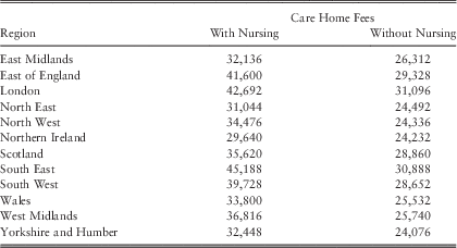
Laing & Buisson (2012/2013).
Average Hourly Daytime In-Home Care Cost (£) by UK Region in 2009/2010
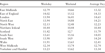
Laing & Buisson (2011).
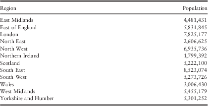
7.2.2. Once the government’s cap has been reached, the individual has no liability for care costs, but still must pay for staying in a care home, for food and for the utilities – the so-called hotel costs. This cost is fixed, regardless of whether there is any nursing care provided. Hancock et al. (Reference Hancock, Wittenberg, Pickard, Comas-Herrera, Juarez-Garcia, King and Malley2007) breaks up the hotel costs from the full cost of staying in a residential care home without nursing care in 2002 as £7,900 per annum and £17,000 per annum, respectively. They based their estimate of hotel cost on the Guarantee Credit component of the UK Pension Credit benefit. We assume the proportions remain the same today, i.e. hotel costs are 46% of residential care home without nursing care, or £12,965.
7.2.3. We consider an institutionalised life without any ADLs or with only an IADL as requiring only residential care. Lives who are in an institution and suffering more than 1-ADL will need the most care so we assign these lives to a residential care home with nursing care. Institutionalised lives with 1-ADL might need a bit less attention but more than lives with no functional disability, so we arbitrarily deem this halfway between the cost of a residential care home with and without nursing care.
7.2.4. The condition for claiming based on functional ability in the LTC market is commonly to suffer from at least 2-ADLs. The costs faced by these lives depends on the number of hours of in-home care required. We leave the number of hours a week as a scenario specific parameter and denote it by H.
7.2.5. For our contract, when a life has been diagnosed with dementia, this will reduce the functional disability requirement to trigger a functional disability claim to 1-ADL. Lives with dementia and >1-ADL are given 2H hours of care a week.
7.2.6. Without the existence of the government cap, payments faced by the individual which do not meet the claim requirements are irrelevant to the insurer. In our market, if the individual pays for care which does not meet the insurance company’s claim underwriting but is included within the government’s cap, this will reduce the insurer’s expected future liability. To simplify the situation, we assume the government and insurer have the same criteria regarding claims and set the care costs in states other than those detailed above to be zero.
7.2.7. A summary of the care costs dependent on the current state in the model depicted in Figure 6 are given in Table 6.
Annual Rates for Care and Hotel Costs for Individuals in Our Insurance Market
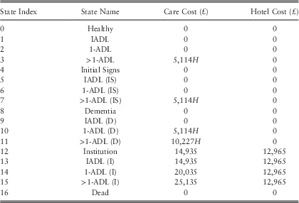
ADL, activity of daily living; IADL, instrumental activity of daily living.
7.3. Initial Distribution of Lives
7.3.1. In our start-up market, we model the progression of the market from introduction of the product. In such a case there will be lives of different ages buying the product and influencing the adverse selection costs. Some lives at each age have already developed some form of cognitive or functional disability so to model forward from the current time, it is necessary to calculate the distribution of lives in each state in our model for each sex, genotype and age group as at 1 January 2013.
7.3.2. We use the distribution of lives at age 60 estimated by Adams (Reference Adams2013), who fitted to functional ability of Akodu (Reference Akodu2007) at later ages using the following assumptions:
a. no lives have any signs of decrease in cognitive function at age 60 – as long-term care is for post-retirement;
b. the size of the population in each age group is estimated by Office for National Statistics (2011) (shown in Table 8); and
c. the mix of APOE genotype is that used by Macdonald & Pritchard (Reference Macdonald and Pritchard2000) and derived by Farrer et al. (Reference Farrer, Cupples, Haines, Hyman, Kukull, Mayeux, Myers, Pericak-Vance, Risch and van Duijn1997) (shown in Table 7).
Distribution of apolipoprotein E gene genotypes
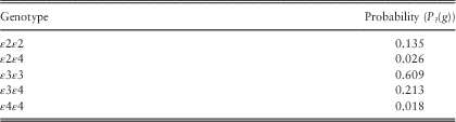
7.3.3. Let  $$N(x,\varsigma )$$
be the number of lives aged x and of sex ϛ based on Table 8,
 $${\cal S}'\!={\cal S}\,$$
\{16} be the set of health states, excluding Dead, and
 $${\cal X}$$
={62.5, 67.5, 72.5, 77.5, 82.5, 87.5} be the set of midpoints of each of our age groups. Using the assumptions and calculated distributions of lives at age 60, we can find the distribution of lives who are alive at age x of sex ϛ with genotype g and are in state j at 1 January 2013,
 $$p_{{x,\varsigma ,g}}^{j} $$
, by calculating
 $$p_{{x,\varsigma ,g}}^{j} ={{\mathop{\sum}\limits_{i=0}^3 P_{{{\rm ADL},\varsigma }} \left( i \right)\:P_{{\cal G}} \left( g \right)\:_{t} p_{{60,\varsigma ,g}}^{{i,j}} \:N(x,\varsigma )} \over {\mathop{\sum}\limits_{y\in {\cal X},\sigma \in \{ M,F\} ,g\in {\cal G},s\in {\cal S}'} \mathop{\sum}\limits_{i=0}^3 P_{{{\rm ADL},\sigma }} \left( i \right)\:P_{{\cal G}} \left( g \right)\:_{t} p_{{60,\sigma ,g}}^{{i,s}} \:N(y,\sigma )}}$$
7.3.4. This will not necessarily produce an accurate depiction of the mix of lives of the UK population, however, the purpose of such a distribution is to provide an approximate baseline from which we can illustrate how adverse selection may impact costs. The aim of our model is not to accurately estimate or project future demand for services and our results should not be used in this way.
7.4. Distribution of Insured Lives
7.4.1. To provide context for adverse selection costs, we consider the joint distribution of insurance purchase time, age and sex, conditional on insurance being purchased. Let T INS, X and  $\sum$
be the random variables representing insurance purchase time, age group and sex, respectively. We denote the joint density function for insurance purchase time, sex and age group, conditional on insurance being purchased by
 $$f_{{T^{{{\rm INS}}} ,\Sigma ,X\,\mid\,T^{{{\rm INS}}} \lt \infty}} (t,\varsigma ,x)$$
, and calculate it as
 $$f_{{T^{{{\rm INS}}} ,\Sigma ,X\,\mid\,T^{{{\rm INS}}} \lt \infty}} (t,\varsigma ,x)={{\mathop{\sum}\limits_{g\in {\cal G},i,j\in {\cal S},\vartheta \in \Bbb B} p_{{x,\varsigma ,g}}^{i} \:_{t} p_{{x,\varsigma ,g}}^{{00i,0\vartheta j}} \:\mu _{{x,t,\varsigma ,g}}^{{0\vartheta j,\vartheta j}} } \over {\mathop{\int}\nolimits_0^\infty \mathop{\sum}\limits_{y\in {\cal X},\sigma \in \{ M,F\} ,g\in {\cal G},i,j\in {\cal S},\vartheta \in \Bbb B} p_{{y,\sigma ,g}}^{i} \:_{_s} p_{{y,\sigma ,g}}^{{00i,0\vartheta j}} \:\mu _{{y,s,\sigma ,g}}^{{0\vartheta j,\vartheta j}} \:ds}}$$
with the integration calculated numerically using Simpson’s rule and a step size of 2−11. The resulting density functions are shown in Figure 8, assuming adverse selection is owing to lives with the initial signs of dementia or 1-ADL buying at a rate of 0.25 per annum.
Joint density function for insurance purchase time, sex and age group, conditional on insurance being purchased. Only plots for lives aged 62.5 at 1 January 2013 are shown, other ages are available in Adams (Reference Adams2013)

7.4.2. We can see that the majority of business is sold during the first 10–15 years; very few lives buy when x+t is >90 years old. There is an interesting feature among both males and females, for x=62.5, whereby there is a local minimum followed by a local maximum for the smaller markets at t=5 and t=15, respectively, for males and t=2 and t=10, respectively, for females. These turning points are because of the changing pattern of health with age: initially, the adverse selectors in this age group are functionally disabled; as dementia onset increases, the adverse selection comes from lives with the initial signs of dementia.
7.4.3. As we are concerned with a start-up market, we choose to model for 20 years. As very few lives purchase insurance after this time (we have not modelled entry to the market from younger lives), the implication of this is limited. Moreover, this is longer than the previous attempt at selling the product in the United Kingdom lasted. If the product is successful, a large body of claims history might allow a more robust analysis, perhaps performed by the CMI, to estimate an insured lives morbidity table that insurers could adjust to suit their own market segment.
8. Analysis of Premium Rates
8.1. In this section we calculate and analyse the premiums that would be charged to lives if the insurer knew all relevant information (applicant’s exact health status, sex and genotype) and was able to underwrite fully, i.e., an underwriting class for each sex, state and genotype combination. This will aid the understanding of the potential sources of adverse selection.
8.2. To do so we run the model from section 2 with assumptions as follows:
a. The insurance contract indemnifies the life up to a maximum lifetime coverage of £200,000, with no annual claim limit.
b. Care costs, other than hotel costs, are capped at £75,000, adjusted for 4 years of inflation at a force of inflation of v=0.04 per annum.
c. The number of hours of in-home care per day for lives with >1-ADL is H=1.
d. There is no deferred period.
e. The force of interest is δ=0.04 per annum.
f. The market size, i.e., the rate at which lives are assumed to buy insurance, is 0.001 per annum.
8.3. The resulting regular premium rates per annum for a life aged 62.5 at 1 January 2013, dependent on purchase time (since the start of our simulation), are shown in Figure 9. Figures for other ages and single premium are not shown, but are available in Adams (Reference Adams2013). Overlayed onto each of these are the premium rates that would be charged if all lives buying insurance were written into one underwriting class for the age group, without any adverse selection in the market (what we termed base premium in section 5 and calculated using equation (30)).
Regular premium rates for long-term care insurance (LTC), assuming the insurer had complete information about the customer and put lives in each age group, sex, genotype and health status into separate underwriting classes, for lives aged 62.5 at 1 January, 2013, against time of purchase (years since market commencement). The same legend is used throughout the plots

8.4. We can see the biggest difference in premium rates is derived from the initial signs of dementia. In addition, if pricing men and women separately, premiums for women are larger than those for men, reflecting the higher rate of dementia found in women.
8.5. Before showing the initial signs of dementia, the premium rates do not differ hugely by genotype. The effect of moving to an initial signs type state increases the premium rates more for females than males. As this is closer to a dementia claim, the effect of genotype becomes more important and differences between premium rates for genotypes are apparent.
8.6. In terms of perceived cheapness of the premiums that would be charged without full information (the thick lines in the figures), at younger ages when the majority of lives have no signs of dementia, premiums are closer to the Healthy rates, so in 1-ADL it appears cheap. For lives with the initial signs of dementia, base premiums represent as much as half of the premium, which they would pay if fully underwritten. As age increases, the proportion of lives with the initial signs of dementia increases and premiums become expensive even for lives with 1-ADL. The high unisex premium caused by female lives’ dementia claims makes the premium seem expensive for males with APOE genotypes ε2ε2, ε2ε4 and ε3ε4. Where people see the premium as cheap, we assume they buy the insurance at a higher rate as they are receiving better value for money and this we see as adverse selection.
8.7. Attention should be drawn to the people who these products would be marketed to: old people who own their own home, but, nonetheless, are living on a pension. Premiums between £1,500 and £2,000 per annum are likely to be seen as a substantial portion of a tight budget.
9. Calculating Adverse Selection
9.1. In this section we consider the impact of lives making the rational decision to either buy LTC insurance at an increased rate when faced with a cheap premium with respect to what they know about their own risk or at a lower rate when premium is expensive. This will be calculated in the context of a new market for the product being created at the modelling date, 1 January 2013. We will show how the cost of adverse selection will develop over time when the insurance company is able to respond to the cashflows it observes from in-force business by adjusting premium rates charged to new business. Each age group is modelled independently of any other so the repricing adjustments relate only to the claims history of the particular cohort.
9.2. The cost of adverse selection may be expressed as a percentage of premium income and defined as
 $${{E{\rm (PV}\,{\rm benefits\,\mid\,Adverse}\ {\rm selection)}{\minus}E{\rm (PV}\ {\rm premium}\ {\rm income\,\mid\,Adverse}\ {\rm selection)}} \over {E{\rm (PV}\,{\rm premium}\ {\rm income\,\mid\,Adverse}\ {\rm selection)}}}$$
where the premium rates charged are calculated using our dynamic approach, assuming no adverse selection for the base premium rates.
9.3. Based on the analysis in section 8, we consider the possibility of higher than expected purchase rates from lives who find they have a high-risk variant of the APOE gene; lives who have observed the initial signs of dementia; and lives in a high-risk ADL state beyond the detection of underwriting capabilities in the scenario. We also allow lives with a low-risk variant of the APOE gene or in the lowest risk state in the class to buy at a lower rate.
9.4. Adverse Selection Sources in Isolation
9.4.1. To demonstrate the relative impact of each source of adverse selection, we model with buying behaviour changing due to one factor at a time. We use the same set of assumptions as above and where the buying rate is high, this is at a rate of 0.25 per annum.
9.4.2. For the purposes of this exercise, we consider high-risk variants of APOE to be ε3ε4 and ε4ε4, while low-risk variants are ε2ε2 and ε3ε3 with testing occurring at a rate of 0.08916 per annum, the high rate from Adams et al. (Reference Adams, Donnelly and Macdonald2013). This is used to exaggerate the costs in order to illustrate how genetic testing interacts with other scenarios. As discussed above, testing for APOE variations in relation to AD is unlikely to be done at the request of physicians, but may be done if an individual uses a personal testing service. Figure 10a shows the repricing adjustment factors to the base premiums, dependent on the time of purchase (measured in years since market commencement), using equation (46) – these are calculated based on the information the insurer gains through its claims history. To provide this with context, Figure 10b shows the adjustments that would be made to the base premiums, if the insurance purchase pattern was exactly the same, and the insurer knew everything about the customer, which was relevant to pricing when the policy was sold – this is the factor by which the base premium should be multiplied to pay for all benefit outgo.
(a) Repricing adjustments made to new business regular premiums through the emerging information from claims history and (b) adjustments that would be made to new business regular premiums if the insurer knew everything relevant about the customer at the point of sale, when a single source of adverse selection is present: “Healthy” – lives in the Healthy state do not buy; “Low Gene” – lives with apolipoprotein E gene genotypes ε2ε2 and ε3ε3 do not buy; “High Gene” – lives with apolipoprotein E gene genotypes ε3ε4 and ε4ε4 buy at an increased rate; “Initial Signs” – lives with initial signs of dementia buy at an increased rate; “1-ADL” – lives with 1-ADL functional disability type buy at an increased rate

9.4.3. What we can observe from these plots is that lives with the initial signs of dementia buying at a higher rate should have the biggest effect on premium rates, although this is overtaken at the oldest ages by lives with 1-ADL. However, the rate at which losses from this source of adverse selection are recognised is slower than that of lives in the Healthy state not buying and lives with 1-ADL buying at a high rate. This means the premiums charged to new business do not increase enough to cover the benefit costs of the business, leaving a larger cost of adverse selection.
9.4.4. We can also see that on its own, genetic testing at this test rate should increase premiums a moderate amount, however, the threat posed by this is small relative to the other potential sources of adverse selection. Overlap between the factors may cause smaller influence from genetic tests than these would suggest. A limitation of the methodology used – lives with particular genotype buy at a higher rate for the remaining period after receiving test results – is that at later ages, the relative risk model used gives the “high-risk” APOEε4 variants, ε2ε4 and ε3ε4 the same relative risk as ε3ε3 in males.
9.5. Multiple Sources of Adverse Selection
9.5.1. In assessing a more complete picture of adverse selection, with more than one source at a time, we will use the following assumptions:
a. The size of the market will be represented by purchase rates of 0.001, 0.01 and 0.05 per annum.
b. Lives who buy at an increased rate will do so at either 0.25 or 0.1 per annum and in the case of the smallest market, at 0.01 per annum also.
c. Underwriters will either group all lives into one class or group lives with 1-ADL in their own class.
d. Lives receiving in-home care will be given either H=1 or H=2 hours of care per day, corresponding to the results of Jones (Reference Jones2006), Forder & Fernández (Reference Forder and Fernández2009)and the assumption in Nuttall et al.’s (Reference Nuttall, Blackwood, Bussell, Cliff, Cornall, Cowley, Gatenby and Webber1994) moderate needs estimate, respectively. Costs of care are as outlined in Table 6.
e. Testing will be performed at a rate of 0.08916 per annum.
f. The force of inflation will be 0.02 or 0.04 per annum, while the force of interest is 0.05.
g. An individual’s care liability will be capped by the government at £75,000, adjusted for 4 years’ inflation.
h. The insurance contract will indemnify the policyholder up to £200,000 with no limit on annual payouts.
i. The relevancy function in equation (45) will be parameterised using β=−0.01 and γ=−0.25.
j. The number of lives of age x and sex ϛ is as in Table 8.
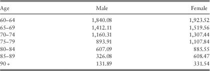
9.5.2. In our modelling we assume adverse purchase rates for males and females are equal. However, this is not necessarily how it would be borne out in practice as the product represents a different value to each sex – females may be expected to have a higher purchase rate as the product represents greater value to them.
9.5.3. We calculate the cost of adverse selection for all business sold in underwriting class k during calendar year c by realising the future losses the business will incur when adverse selection is present, and discounting these to start of year c. We assume the premiums are calculated using the claims history to apply a repricing adjustment to the base premiums, the latter calculated assuming no adverse selection. By expressing the loss as a percentage of premium income, we show how much further the premiums need to be increased, in order to reach the actuarially fair premiums that were intended. Benefit outgo and premium income arising from business sold to lives aged x at 1 January 2013, are weighted by the number of lives in that age group. This can be expressed as
 $$\eqalignno{ {\rm Adverse}\ {\rm selection}\ {\rm cost} & ={{E({\rm PV}\ {\rm benefits}{\minus}{\rm PV}\ {\rm premium}\!\mid\!{\rm Adverse}\ {\rm selection})} \over {E({\rm PV}\ {\rm premium}\!\mid\!{\rm Adverse}\ {\rm selection})}} \cr & ={{\mathop{\sum}\limits_{x\in {\cal X},\varsigma \in \{ M,F\} ,g\in {\cal G},i\in {\cal S},j\in {\cal U}_{k} ,\vartheta \in \Bbb B} \mathop{\int}\limits_c^{c{\plus}1} {p_{{x,\varsigma ,g}}^{i} _{t} \tilde{p}_{{x,\varsigma ,g}}^{{00i,0\vartheta j}} \tilde{\mu }_{{x,t,\varsigma ,g}}^{{0\vartheta j,1\vartheta j}} \left( {A_{{x,\varsigma ,g,t:c}}^{{j,P}} {\minus}\overline{\Pi } _{{x,t}}^{k} a_{{x,\varsigma ,g,t:c}}^{{j,P}} } \right)dt} } \over {\mathop{\sum}\limits_{x\in {\cal X},\varsigma \in \{ M,F\} ,g\in {\cal G},i\in {\cal S},j\in {\cal U}_{k} ,\vartheta \in \Bbb B} \mathop{\int}\limits_c^{c{\plus}1} {p_{{x,\varsigma ,g}}^{i} _{t} \tilde{p}_{{x,\varsigma ,g}}^{{00i,0\vartheta j}} \tilde{\mu }_{{x,t,\varsigma ,g}}^{{0\vartheta j,1\vartheta j}} \overline{\Pi } _{{x,t}}^{k} a_{{x,\varsigma ,g,t:c}}^{{j,P}} dt} }}$$
9.5.4. We start by considering adverse selection costs when lives with the initial signs of dementia and lives with 1-ADL buy at an increased rate without any underwriting. The progression of these costs, dependent on time of purchase (measured in years since market commencement), are shown in Figure 11 for regular and single premium on unisex and gender-specific bases with H=1 and v=0.04.
Progression of adverse selection cost when lives with the initial signs of dementia or 1-ADL buy insurance at an increased rate with H=1, v=0.04. The government does not cap care liability

9.5.5. The patterns shown are much the same, regardless of the premium basis: very high costs attributable to business sold at the start of the market, while policies sold after 20 years since market set-up have negative costs. These negative costs reflect the repricing process increasing premiums too much – referring back to Figure 10b, we see the premium adjustments that should be gradually decreased, which is because of the base premium accommodating a greater proportion of higher risk lives without adverse selection. Losses are noticed more rapidly when the purchase rate for adverse selectors is highest, and despite being the highest cost initially, the smallest market with high adverse purchase rate responds quickest and becomes the most negative. The regular premium version of the contract has ∼30% higher costs initially and these costs become more negative when policies are being charged too much.
9.5.6. There are a number of uncertain parameters involved in our model. To assess how the choice of value of these parameters might influence results, we present some analysis of the sensitivity.
9.5.7. The sensitivity of adverse selection costs over time to the inflation rate parameter can be seen in Figure 12 to be very low – the shape of the emergence over time and the size are very similar. As the highest costs are at the start of the market, before the insurer has been able to adjust they correct their pricing assumptions, when the inflation rate is higher (and consequently the real discount rate lower) the smaller cost incurring/profit making business in the latest years is given more weight making the overall adverse selection cost, as a percentage of premium income, lower.
Sensitivity of adverse selection costs to number of hours of care provision and the force of inflation when lives with the initial signs of dementia and lives with 1-ADL buy insurance at an increased rate and premiums are charged on a unisex basis: (a) H=1, INF=0.02; (b) H=2, INF=0.02; and (c) H=2, INF=0.04

9.5.8. Figure 12 also shows the sensitivity to the number of hours of in-home care provision, H. Increasing H from 1 to 2 decreases the adverse selection cost. This may seem counter intuitive as we have lives at risk of claiming in-home care provision buying at an increased rate. However, as noted above, the biggest part of adverse selection cost is from lives observing the initial signs of dementia. These lives are also exposed to the parameter H, pre-institutionalisation but once they have been institutionalised, their care costs are no longer based on H. Consequently, although overall benefit costs are higher when H=2, the increased premium rate offsets some of the adverse selection costs. As the shape of the development of the costs does not change markedly, only the scale, we continue in this section with H=1.
9.5.9. Now when we include adverse selection from lives who have had a genetic test (shown in Figure 13), the effect is twofold: initially the costs are lower with genetic adverse selection owing to lives with high-risk genes buying insurance earlier than they would when they move to a state where the difference between their benefit costs and premium income is greater; at later purchase times, the adverse selection cost is higher with genetic adverse selection because losses owing to genetic adverse selection are realised slowly (see Figure 10a) so premiums have not been changed sufficiently. In the large market, this creates a local minimum and subsequently a local maximum for males and where premiums are unisex.
Progression of adverse selection cost when lives with the initial signs of dementia or 1-ADL buy insurance at an increased rate and lives change buying behaviour after having a genetic test, with H=1, v=0.04

9.5.10. If the market fails to attract lives in the Healthy state but lives with the initial signs or 1-ADL buy at an increased rate there will be little difference between the market sizes (see Figure 14) as only the relatively small proportion of lives with an IADL buy at the standard market rate. The effect of genetic testing in this case is minimal as the only lives in the IADL state will change buying behaviour owing to test results.
Progression of adverse selection cost when lives with the initial signs of dementia or 1-ADL buy insurance at an increased rate and lives change buying behaviour after having a genetic test, while healthy lives do not buy insurance regardless of genotype, with H=1, v=0.04

9.5.11. The scenarios above have assumed there is a restriction on underwriting. If we permit insurers to underwrite based on functional ability, as would be the case in the United Kingdom, there would be no reason for lives with 1-ADL to purchase insurance at an increased rate, merely because of their functional disability.
9.5.12. As our model is Markov, a life’s health history (beyond its current state) tells nothing of its future health. Therefore, when a life has been underwritten into a high-risk class, if the life subsequently recovers they could lapse their policy and buy another written in a lower-risk class with a correspondingly lower premium. This is a consideration that would be necessary only when charging regular premiums, similar to the problem mentioned in section 8.
9.5.13. The results of introducing underwriting are shown in Figure 15 when lives with the initial signs of dementia buy insurance at an increased rate and change buying behaviour after the result of a genetic test. Despite eliminating functional ability as a source of adverse selection, the costs as a percentage of premium income have increased when we compare with Figure 13, particularly for females and the smaller market sizes. This should be expected because the biggest part of adverse selection cost is from the insurer being unable to discern between lives with and without the initial signs of dementia. This still remains, while lives in the “low-risk” underwriting class pay a smaller premium than without underwriting. Hence, the nominal amount of loss has decreased, but less than the nominal amount of premium income has. In addition, the local maximum observed upon introducing genetic adverse selection is more pronounced and exists for the other market sizes. Losses owing to adverse selection from 1-ADL are realised relatively rapidly hence increased premiums can be used to cover losses from high purchase rates from lives with initial signs of dementia that are realised more slowly.
Progression of adverse selection cost when lives with 1-ADL are written into a separate class while lives with the initial signs of dementia buy insurance at an increased rate and lives change buying behaviour after having a genetic test, with H=1, v=0.04

9.6. Varying the Caps
9.6.1. We have used a cap on care costs before the government takes on the liability assuming £75,000 in 2017, as per the Westminster government’s stated intentions. If this does not get approval of parliament, there will be no cap on the liability faced by the individual. Moreover, we have not considered the situation in Scotland, where care costs are intended to be met by the Scottish government. We examine these extremes of policy here.
9.6.2. First, we consider the Scottish government’s policy and assume that their payment is sufficient to meet the care costs. The adverse selection costs (shown in Figure 16) as a percentage of premium are substantially larger than those where the insurance policy also pays for care costs. In this situation, the role of the insurance policy is to meet the hotel costs, a benefit only associated with dementia. Correspondingly, benefit sizes are smaller and the probability of reaching a claim is reduced, hence the premiums are also reduced. This smaller premium base, as we have seen above (in the scenario with underwriting), creates large adverse selection costs.
Progression of adverse selection cost when lives with the initial signs of dementia or 1-ADL buy insurance at an increased rate with H=1, v=0.04. Insurance pays for hotel costs only

9.6.3. Next we look at adverse selection costs if the UK government does not implement their proposed cap. These are shown in Figure 11. Comparing these with the equivalent scenario with the cap, in Figure 17, we see very little impact from the removal of the cap on care costs.
Progression of adverse selection cost when lives with the initial signs of dementia or 1-ADL buy insurance at an increased rate with H=1, v=0.04

9.6.4. To investigate this further, we amended our simulation model to estimate the distribution of total care individuals face over their lifetime. For each sex, genotype and health state, we simulated the future life histories and the associated care costs of 1,000,000 lives aged  $x\in {\cal X}$
. Where the total care costs for lives was non-zero, these were separated into “bins” of size £1,000 in terms of 1 January 2013’s purchasing power. A further bin existed for lives who never had any care expenditure. Summing the number of lives in each bin over genotypes
 $g\in {\cal G}$
and states
 $j\in {\cal S}$
, with weighting equal to the probability for the initial distribution,
 $$p_{{x,\varsigma ,g}}^{j} $$
(calculated in section 6), allows us to estimate a distribution for a discretised care cost, for a particular age group x and sex ϛ.
9.6.5. The nature of adverse selection means that in our pool of insurance business, the mix of lives who buy insurance does not match the mix of lives in the general population – there will be a higher proportion of lives who require care. As a proxy for the mix of insured business, we consider the distribution of care costs, conditional on the care cost being non-zero. Denote the number of lives aged x of sex ϛ with genotype g and in state j at 1 January 2013, whose simulated care costs were between 1,000i and 1,000(i+1), by  $$b_{{x,\varsigma ,g}}^{j} (i)$$
. For lives aged x, of sex ϛ, we estimate the probability mass function of care costs, conditional on the cost of care being non-zero, as
 $$P(1,000i\,\lt\, {\rm Care}\,{\rm cost}\,\leq\, 1,000(i{\plus}1)\!\mid\!{\rm Care}\,{\rm cost}\,\gt\, 0){\rm =}{{\mathop{\sum}\limits_{g\in {\cal G},j\in {\cal S}} p_{{x,\varsigma ,g}}^{j} b_{{x,\varsigma ,g}}^{j} (i)} \over {\mathop{\sum}\limits_{g\in {\cal G},j\in {\cal S},k\in N} p_{{x,\varsigma ,g}}^{j} b_{{x,\varsigma ,g}}^{j} (k)}}$$
For ages 62.5 and 87.5, this is shown in Figure 18.
Probability density functions of care costs, conditional on the cost of care being non-zero, separated by age and sex

9.6.6. The adverse selection we have considered does not impact upon the duration of care requirements. We therefore suggest the distribution of care costs would not differ greatly between what is anticipated in pricing and what is experienced. As only a small proportion of lives are affected by the removal of the cap (see Table 9), where a difference in this distribution were to arise, the associated loss would not be large when spread over a portfolio of business. This explains why the changes in costs of adverse selection were so small when the government cap was removed.
Conditional Probabilities of Reaching the UK Government’s Proposed Care Cap of 75,000, Adjusted for 4 Years’ Inflation, Assuming a Force of Inflation of v=0.04 Per Annum
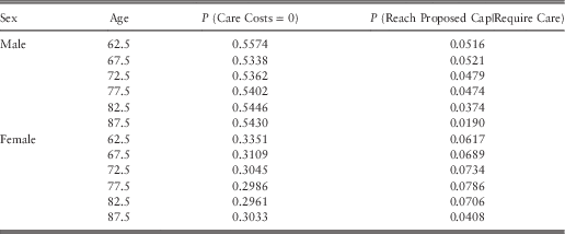
10. Cross-Subsidy in Unisex Premiums
10.1. As noted in section 8, premiums for females are substantially higher than those for males when using sex as a pricing factor. Hence, under a unisex format where the costs are spread over both sexes, males will be paying more than they otherwise would.
10.2. Define the cross-subsidy to be the excess of premium income from one group (call this group A) over the benefits paid to them used to cover losses on business from another group (call this group B):
 $${\rm Cross{\hyphen}subsidy=}\left\{ {\matrix{ {{\rm Profit}\ {\rm from}\ A{\rm ,}} & {{\rm if}\ 0\,\lt\, \,{\rm Profit}\ {\rm from}\ A\,\leq\, {\rm Loss}\ {\rm from}\ B} \cr {{\rm Loss}\ {\rm from}\ B{\rm ,}} & {{\rm if}\ 0\,\lt\, \,{\rm Loss}\ {\rm from}\ B\,\lt\, {\rm Profit}\ {\rm from}\ A} \cr {0,} & {{\rm otherwise}} \cr } } \right.$$
For the existence of a cross-subsidy, it is therefore necessary for a simultaneous occurrence of both profit from one group of lives and losses from the other.
10.3. When the mix of lives matches what is priced for, this will create a cross-subsidy that is measurable simply by comparing the premium rates in Figure 9. However, in the context of adverse selection, this cross-subsidy may disappear if premium income from males is insufficient to cover the benefits males receive or if the premium adjustment is such that females’ benefits are fully covered by females’ premiums. In this section we analyse the premium income and benefit payments at the level of particular sex to quantify the cross-subsidy in the unisex premiums. In this case group A are the male lives and group B are the female lives.
10.4. We can calculate the profit from males aged x in 2013, who purchased insurance in calendar year c, which we denote by  $$\overline{A} (x,c)$$
and A(x, c), for regular and single premium versions, respectively, as
 $$\bar{A}(x,c){\rm =}\mathop{\sum}\limits_{g\in {\cal G},i\in {\cal S},j\in {\cal U}_{k} ,\vartheta \in \Bbb B} \mathop{\int}\limits_c^{c{\plus}1} {p_{{x,M,g}}^{i} _{t} \tilde{p}_{{x,M,g}}^{{00i,0\vartheta j}} \tilde{\mu }_{{x,t,M,g}}^{{0\vartheta j,1\vartheta j}} \left( {\overline{\Pi } _{{x,t}}^{k} a_{{x,M,g,t:c}}^{{j,P}} {\minus}A_{{x,M,g,t:c}}^{{j,P}} } \right)dt} $$
and
 $$A(x,c){\rm =}\mathop{\sum}\limits_{g\in {\cal G},i\in {\cal S},j\in {\cal U}_{k} ,\vartheta \in \Bbb B} \mathop{\int}\limits_c^{c{\plus}1} {p_{{x,M,g}}^{i} _{t} \tilde{p}_{{x,M,g}}^{{00i,0\vartheta j}} \tilde{\mu }_{{x,t,M,g}}^{{0\vartheta j,1\vartheta j}} \left( {\Pi _{{x,t}}^{k} {\minus}A_{{x,M,g,t:c}}^{{j,P}} } \right)dt} $$
Similarly, we calculate the loss from females aged x in 2013, who purchased insurance in calendar year c, which we denote by  $$\overline B(x,\,t)$$
and B(x, t) as
 $$\overline{B} (x,\,c)=\mathop{\sum}\limits_{g\in {\cal G},\,i\in {\cal S},\,j\in {\cal U}_{k} ,\,\vartheta \in \Bbb B} \mathop{\int}\limits_c^{c{\plus}1} {p_{{x,\,F,\,g}}^{i} _{t} \tilde{p}_{{x,\,F,\,g}}^{{00i,\,0\vartheta j}} \tilde{\mu }_{{x,\,t,\,F,\,g}}^{{0\vartheta j,\,1\vartheta j}} \left( {A_{{x,\,F,\,g,\,t:c}}^{{j,\,P}} {\minus}\overline{\Pi } _{{x,\,t}}^{k} a_{{x,\,F,\,g,\,t:c}}^{{j,\,P}} } \right)dt} $$
and
 $$B(x,\,c)=\mathop{\sum}\limits_{g\in {\cal G},\,i\in {\cal S},\,j\in {\cal U}_{k} ,\,\vartheta \in \Bbb B} \mathop{\int}\limits_c^{c{\plus}1} {p_{{x,\,F,\,g}}^{i} _{t} \tilde{p}_{{x,\,F,\,g}}^{{i,\,j}} \tilde{\mu }_{{x,\,t,\,F,\,g}}^{{j,\,{\rm INS}}} \left( {A_{{x,\,F,\,g,\,t:c}}^{{j,\,P}} {\minus}\Pi _{{x,\,t}}^{k} } \right)dt} $$
for regular and single premium versions, respectively.
10.5. Let the cross-subsidy across all business sold in calendar year c, expressed as a percentage of male premium, be denoted by  $$\Pi _{{x,t}}^{k} $$
and χ(c) and calculated as
 $$\bar{\chi }(c){\rm =}{{\min \left[ {\max \left( {0,\,\mathop{\sum}\limits_{x\in {\cal X}} \overline{A} (x,\,c)} \right),\,\max \left( {0,\,\mathop{\sum}\limits_{x\in {\cal X}} \overline{B} (x,\,c)} \right)} \right]} \over {\mathop{\sum}\limits_{x\in {\cal X},\,g\in {\cal G},\,i\in {\cal S},\,j\in {\cal U}_{k} ,\,\vartheta \in \Bbb B} \mathop{\int}\limits_c^{c{\plus}1} {p_{{x,\,M,\,g}}^{i} _{t} \tilde{p}_{{x,\,M,\,g}}^{{00i,0\vartheta j}} \tilde{\mu }_{{x,\,t,\,M,\,g}}^{{0\vartheta j,1\vartheta j}} \overline{\Pi } _{{x,c}}^{k} \:a_{{x,\,M,\,g,\,t:c}}^{{j,P}} dt} }}$$
and
 $$\chi (c)={{\min \left[ {\max \left( {0,\,\mathop{\sum}\limits_{x\in {\cal X}} A(x,\,c)} \right),\,\max \left( {0,\,\mathop{\sum}\limits_{x\in {\cal X}} B(x,\,c)} \right)} \right]} \over {\mathop{\sum}\limits_{x\in {\cal X},\,g\in {\cal G},\,i\in {\cal S},\,j\in {\cal U}_{k} ,\,\vartheta \in \Bbb B} \mathop{\int}\limits_c^{c{\plus}1} {p_{{x,\,M,\,g}}^{i} _{t} \tilde{p}_{{x,\,M,\,g}}^{{00i,\,0\vartheta j}} \tilde{\mu }_{{x,\,t,\,M,\,g}}^{{0\vartheta j,\,1\vartheta j}} \Pi _{{x,\,c}}^{k} dt} }}$$
for regular and single premium versions, respectively.
10.6. We analyse the cross-subsidies in two of the scenarios from section 9, corresponding to Figures 11 and 15, respectively.
10.7. Figure 19a shows the progression of the cross-subsidy when lives with the initial signs of dementia or 1-ADL buy insurance at an increased rate. There is an inverse relationship between cost of adverse selection and the cross-subsidy – while adverse selection cost is high, it is unlikely there is a profit being made from males and when adverse selection cost is negative, it is possible that there is no loss on female business. Consequently, the large market has the greatest cross-subsidy and is non-zero throughout. Smaller market sizes make a loss on both male and female business initially, so have no cross-subsidy. This lasts longer under the regular premium product than the single premium version.
Progression of the cross-subsidy from males in unisex premiums when (a) lives with the initial signs of dementia or 1-ADL buy insurance at an increased rate and (b) lives with 1-ADL are written into a separate class while lives with the initial signs of dementia buy insurance at an increased rate and lives change buying behaviour after having a genetic test. In both cases H=1, v=0.04, and black indicates the cross-subsidy is the profit on males, while grey indicates that it is the loss from females

10.8. In Figure 19b we have lives with 1-ADL being underwritten into a separate class of business. Lives with the initial signs of dementia buy insurance at an increased rate and lives alter buying behaviour after a genetic test. In this case, a cross-subsidy initially exists in the large market but becomes zero around year 15. Other market sizes see a cross-subsidy once premiums have been adjusted: in the single premium version, cross-subsidy exists for all cases but is short-lived for all but the lowest rate of adverse selection in the small market; under a regular premium, cross-subsidy only exists in the smallest market in the final years, and lasts for a short time in market with purchase rate 0.01.
11. Conclusions
11.1. Renewed interest in long-term care from the government, and coverage in the press, highlighting the need for reform, and has made the prospect of creating a new LTC market in the United Kingdom a possibility. Adverse selection has been suggested as a potential barrier to the success of such a market. This adverse selection could come from lives who have had their APOE genotype tested, have the initial signs of dementia, are healthy, or depending on underwriting practice, have some functional disability.
11.2. Our dynamic pricing strategy allows insurers to correct their premiums. We have seen that losses from dementia are realised slower than losses from functional ability, but it is dementia where the greatest adverse selection costs arise.
11.3. These costs vary greatly over time. The reason for this is twofold: the insurer adjusts its premium rates to factor in its experience; and the base premiums assume increasing proportions of the high-risk lives – who are adversely selecting. In the early years of the market, where the majority of the modelled lives purchase their contract, they can reach significantly large levels. In the context of large premiums on contracts being sold to pensioners on tight budgets, any increase of premiums to pay for adverse selection would present challenges in marketability.
11.4. On its own and with an exaggerated rate of testing, genetic testing poses a moderate cost which is dwarfed when compared with the other potential sources of adverse selection. As a large proportion of lives with the initial signs of dementia progress to large claims, they were also responsible for the largest adverse selection costs. When other sources of adverse selection were included, in addition to the initial signs of dementia, adverse selection costs were decreased because the selection was able to occur earlier, when lives were of a slightly lower risk. Moreover, claims from lives with functional disability adversely selecting, allowed the repricing mechanism to increase premiums to cover some of the losses to be incurred from the dementia claims.
11.5. The adverse selection costs are insensitive to movements of inflation and to the level of benefits paid for functional disability. While an improvement in the size of the government’s cap on care liability changes adverse selection costs significantly, removing the cap made very little impact. We found this was owing to there being a small percentage of lives benefiting from the introduction of such a cap. How well this meets the needs of citizens is a matter for social policy researchers to consider and politicians to debate. However, actuaries will be interested in the extent that it removes tail risk, which our results cannot say anything about.
11.6. Within unisex premiums for LTC, there is a high degree of cross-subsidy from males to pay for the higher benefit costs of females. LTC is not unique in such a cross-subsidy, a common example of a contract with one being motor insurance (where females subsidise males), but introducing a new product with cross-subsidy may make selling to men difficult. Whereas, our pricing responds immediately to differences between the genders, an insurer might take somewhat longer.
12. Further Work
12.1. Our model of an LTC market is dynamic from the perspective of the insurance company, in that it reflects the repricing activity that could be made based on claims and income experience. However, we do not make any consideration for where a buying behaviour might change in response to the relative cheapness of the premium rates, beyond simple deterministic scenarios. These could be improved by applying some form of decision-making methodology, such as utility theory or prospect theory or using an elastic model of demand with a suitably parameterised price elasticity based on solid empirical data.
12.2. Given the high costs from adverse selection and the uncertainty over purchasing patterns, it is likely that there is a large risk inherent in writing LTC contracts. To quantify this risk, the LTC simulation model could be amended to calculate the distributions of benefit payments. From these distributions and a suitable model of purchases, measures of risk including value at risk could be calculated that would aid in understanding the risk of the product and how it is influenced by adverse selection. This would be especially important in the context of a risk-based capital requirement regime such as Solvency II. Product designs that share the insurance risk with the policyholder such as with-profits or reviewable premiums could act to reduce the capital requirements. How well these types of products meet the needs of the customer would need further research, in a similar approach to that taken by Guillén & Comas-Herrera (Reference Guillén and Comas-Herrera2012) in Spanish LTC products.
12.3. The direction of genetic research is moving towards analysing the function of risk genes, to understand how they cause predisposition to particular diseases. Such improved understanding might in turn lead to the further development of genomic medicine. Advances in genomic medicine have been slow to surface, but a recent review by Manolio et al. (Reference Manolio, Chisholm, Ozenberger, Roden, Williams, Wilson, Bick, Bottinger, Brilliant, Eng, Frazer, Korf, Ledbetter, Lupski, Marsh, Mrazek, Murray, O’Donnell, Rader, Relling, Shuldiner, Valle, Weinshilboum, Green and Ginsburg2013) is optimistic about its future if more collaboration were to take place. Moreover, recent results from the second Cognitive Function and Ageing Study reported by Matthews et al. (Reference Matthews, Arthur, Barnes, Bond, Jagger, Robinson and Brayne2013) showed a significant decrease in prevalence of dementia. They interpreted this as providing evidence for a cohort effect in dementia prevalence. Actuaries will need to adapt their modelling in line with where the epidemiology leads, whether this could mean the use of multi-factorial models that include the additional factors of, e.g., cigarette smoking or weight, or how developments lead to changing patterns of morbidity over time.
Acknowledgements
This work was carried out at the Genetics and Insurance Research Centre at Heriot-Watt University. The authors would like to thank the sponsors for funding, Bill Baker for his very useful insight into the UK LTC market and Gareth Colgan for his input on post-dementia transitions.