1. Introduction
1.1. Literature review and recent development
Fluids are distinguished from any other continuous media by their constitutive inability to resist shear, which inherently induces rotation of elementary fluid elements (encompassing material lines, surfaces and volumes). This distinctive characteristic is precisely what renders fluid motion exhibiting unparalleled complexity compared with solid continuum mechanics. The symmetric–antisymmetric decomposition (SAD) affirms that the velocity gradient tensor (VGT),
 $\boldsymbol{A}\equiv \boldsymbol{\nabla }\boldsymbol{u}$
, can be decomposed into the strain-rate tensor
 $\boldsymbol{D}$
and the rotation-rate tensor
 $\boldsymbol{\varOmega }$
, such that
 $\boldsymbol{A}=\boldsymbol{D}+\boldsymbol{\varOmega }$
(Batchelor Reference Batchelor1967; Wu, Ma & Zhou Reference Wu, Ma and Zhou2015). Then, the vorticity
 $(\boldsymbol{\omega }\equiv \boldsymbol{\nabla }\times \boldsymbol{u})$
, defined as the curl of the velocity field, emerges naturally as the dual vector of
 $\boldsymbol{\varOmega }$
, providing a kinematic measure for the shear-driven transverse processes in complex flows. In contrast to the momentum description employing the primitive hydrodynamic variables (velocity and pressure), vorticity-based formulations usually offer superior physical intuition and mathematical elegance for complex fluid motions. The vorticity paradigm has been proven to be powerful for analysing the ubiquitous hydrodynamic phenomena like Rayleigh–Taylor and Richtmyer–Meshkov instabilities, with broad applications across geophysical flows to engineering systems (Wu et al. Reference Wu, Ma and Zhou2015; Zhou Reference Zhou2017). Historically, the concept of fluid rotation traces its origins to the classical Cauchy–Stokes theorem (Cauchy Reference Cauchy1841; Stokes Reference Stokes1845), which formalized the local kinematic decomposition of fluid motion via the SAD (Truesdell Reference Truesdell1954). By analogous to rigid-body kinematics, the theorem asserts that the vorticity is just twice the angular velocity of a fluid volume element (Truesdell Reference Truesdell1954; Batchelor Reference Batchelor1967; Corrsin & Karweit Reference Corrsin and Karweit1972), which becomes a cornerstone of modern vorticity and vortex dynamics. However, a lesser-recognized aspect is that the fundamental theory of fluid rotation has evolved along two distinct yet deeply interconnected conceptual pathways, remaining subject to ongoing investigation and not yet finished even today.
The first line of development focuses on three key aspects: the rotation of a fluid volume element; the intrinsic vorticity splitting; and developing the effective criteria for vortex identification. The concept of vorticity was realized insufficient for fully characterizing the vortex motion after the groundbreaking work of Helmholtz in 1858 (English translation version of Helmholtz (Reference Helmholtz1867)), where the word ‘rotation’ was used for half of the vorticity. (The concept of vorticity was first used by Lord Kelvin to describe local rotational motion, though without a rigorous mathematical definition (Thomson Reference Thomson1878). Later, Lamb (Reference Lamb1916) formally introduced the term ‘vorticity’ for
 $\boldsymbol{\omega }$
in the fourth version of his monograph ‘Hydrodynamics’. The components of
 ${1}/{2}\boldsymbol{\omega }$
were called the angular velocities by Stokes (Reference Stokes1851), rotationsgeschwindigkeiten by Helmholtz (Reference Helmholtz1858), the component rotations by Thomson (Reference Thomson1869), the molecular rotations by Basset (Reference Basset1888) and the spin by Clifford (Reference Clifford1878), see Truesdell (Reference Truesdell1954).) As noted by Truesdell (Reference Truesdell1954, § 29), Joseph Bertrand (a French mathematician and physicist) made an observation in 1868 (another way of expressing the rotational character of Bertrand’s shearing motion was put forward by de St. Venant (Reference de Saint-Venant1869) (in a footnote of Truesdell (Reference Truesdell1954)): the straight streamlines are the only lines in the
 $(x,y)$
plane which are not suffering motion) that simple shear flow exhibits non-zero vorticity despite lacking any intuitive swirling motion of a typical vortex – flow particles move in rectilinear trajectories – clearly highlighting a critical limitation in equalling vorticity with vortex. To some extent, this example underscores two crucial insights: (i) swirling motion, a hallmark of vortices, generally contributes to part of vorticity and disappears entirely in simple shear flow; (ii) vorticity is not an appropriate physical measure to represent vortex in shear-dominated region. Standpoint (ii) also applies to turbulent boundary layers: the association between regions of strong vorticity and actual vortices can be rather weak, especially in the near-wall region (Robinson Reference Robinson1991). As the controversy was finally settled, one has realized the necessity of rationally distinguishing between the two elementary vorticity modes, that is, the rigid-rotation mode (swirling-dominant) and the spin mode (shear-dominant), even for a fluid volume element without preferred spatial directionality. Indeed, Prandtl’s boundary layer at high Reynolds numbers is the most brilliant example of the spin-dominated vortical flow. As profoundly articulated by Professor Shijia Lu (1911–1986), the pioneering Chinese aerodynamicist and the sole female student of Ludwig Prandtl (1875–1953) at Göttingen, during her late career, circa 1980: ‘The essence of fluid is vortices. A fluid cannot stand rubbing; once you rub it there appear vortices’ (Wu, Ma & Zhou Reference Wu, Ma and Zhou2006). This rubbing process between fluid and wall creates the boundary layer mediated by viscosity and the no-slip boundary condition. Once an attached boundary layer leaves a solid wall to become a free shear layer (governed by the Biot–Savart law), it can automatically roll into an axial vortex dominated by the rigid-rotation mode, or vice versa, and in such processes vorticity is transferring and redistributed between the two elementary modes (Wu et al. Reference Wu, Ma and Zhou2015; Mao et al. Reference Mao, Li, Yao and Wu2023).
Vortices are the sinews and muscles of fluid motion (Küchemann Reference Küchemann1965), despite the challenges in their precise and universal definition (Lugt Reference Lugt1979; Saffman Reference Saffman1992; Wu et al. Reference Wu, Ma and Zhou2006). Over the past few decades, numerous local vortex identification criteria have been proposed to visualize coherent structures in turbulent flows, with most methods relying on the VGT
 $\boldsymbol{A}$
. Among them, the widely used ones include the vorticity number
 $m$
(Truesdell Reference Truesdell1954), the
 $Q$
-criterion (Hunt, Wray & Moin Reference Hunt, Wray and Moin1988; Jeong & Hussain Reference Jeong and Hussain1995),
 $\varDelta$
-criterion (Chong, Perry & Cantwell Reference Chong, Perry and Cantwell1990),
 $\lambda _{2}$
-criterion (Jeong & Hussain Reference Jeong and Hussain1995) and
 $\lambda _{\textit{ci}}$
-criterion (Zhou et al. Reference Zhou, Adrian, Balachandar and Kendall1999), etc. The Okubo–Weiss criterion (Okubo Reference Okubo1970; Weiss Reference Weiss1991), prevalent in oceanography and atmospheric studies, can be regarded as a two-dimensional (2-D) reduction of the classical
 $Q$
-criterion. However, the flow structures identified by these methods are often highly sensitive to arbitrary threshold selection. Determining an appropriate threshold is challenging, as different values yield significantly different vortical structures (Liu et al. Reference Liu, Gao, Tian and Dong2018; Liu & Wang Reference Liu and Wang2020). Furthermore, they can neither unambiguously determine the swirling axis of a vortex, nor can they elucidate the physical constituents of distinct vorticity modes from vorticity alone. In fluids with small viscosity, the rolling-up of thin shear layers is the only known mechanism for the rapid formation of axial vortices. This physical mechanism arises from extremely strong coupling of longitudinal and transverse fields, which we refer to as the Klein–Kaden–Betz (KKB) mechanism (Klein Reference Klein1910; Kaden Reference Kaden1931; Betz Reference Betz1950; Wu et al. Reference Wu, Ma and Zhou2006; Mao et al. Reference Mao, Li, Yao and Wu2023). These criteria exclude sheet vortices, preventing the KKB mechanism from being fully captured. In addition to the mentioned Eulerian vortex identification methods, Haller & Beron-Vera (Reference Haller and Beron-Vera2013) proposed a variational principle for identifying coherent Lagrangian vortex boundaries in 2-D turbulence, where the solutions are mathematically equivalent to photon spheres surrounding black holes in cosmology.
The rational characterization of these two distinct vorticity modes (i.e. rigid rotation and spin) had long remained ambiguous until Kolář (Reference Kolář2004), in looking for advanced axial-vortex criterion, recalled one’s attention to this fundamental issue. He insisted that ‘solely vorticity cannot distinguish between swirling motions and shearing motions’, leading to the triple decomposition of motion for the VGT
 $\boldsymbol{A}$
(Kolář Reference Kolář2004; Kolář & Savory Reference Kolář and Savory2007; Kolář Reference Kolář2007). Building on the Schur transform (Schur Reference Schur1909), the first version of the normal-nilpotent decomposition (NND-I) of
 $\boldsymbol{A}$
was proposed within a pure algebraic framework (Li Reference Li2010; Li, Zhang & He Reference Li, Zhang and He2014; Liu et al. Reference Liu, Gao, Tian and Dong2018; Gao & Liu Reference Gao and Liu2019). Importantly, NND-I implies the Liutex-shear decomposition for vorticity, which cleanly extracts the characteristic rigid-rotation mode (Liutex/Rortex) to represent vortex, with the residual shear being separated simultaneously (Liu et al. Reference Liu, Gao, Tian and Dong2018; Liu & Wang Reference Liu and Wang2020). To avoid calculating the coordinate rotation matrices, an explicit method for determining the Liutex was proposed by Xu et al. (Reference Xu, Gao, Deng, Liu and Liu2019) and Wang et al. (Reference Wang, Gao, Liu and Liu2019). While NND-I (the Liutex-vector method) has been successfully applied to identify coherent vortex structures in turbulence (Liu & Wang Reference Liu and Wang2020), it is observed that the rigid-rotation mode is limited to regions where
 $\varDelta \gt 0$
which disappears for
 $\varDelta \lt 0$
(with
 $\varDelta$
being the discriminant of the characteristic equation of
 $\boldsymbol{A}$
). It is noteworthy that the matrix of
 $\boldsymbol{A}$
in Nakayama (Reference Nakayama2017) essentially represents a real Schur form for
 $\varDelta \gt 0$
, albeit without introducing the concept of vorticity decomposition. Two physical properties termed ‘swirlity’ and ‘sourcity’ were derived, which, respectively, reflect the symmetry of the vortical flow in the swirl plane and inflowing (outflowing) motion in all directions around a point. Recent work by Li (Reference Li2024) has clarified several confusing points about Schur forms and NND variants, which include the conceptual distinction between NND and triple decomposition of motion approaches, the intrinsic gap between complex and real NND formulations. An improved real Schur form (denoted as NND-II) extends the definition of rigid-rotation mode to all flow regions regardless of the sign of
 $\varDelta$
, with unique matrix representation under proper conditions of uniqueness. However, discontinuity issues and sign ambiguities associated with the two vorticity modes are found when applying NND-II to global flow diagnosis (Chen & Liu Reference Chen and Liu2025), while its physical interpretation remains incomplete under the pure algebraic framework. Furthermore, as noted by Li (Reference Li2024), additional real NNDs beyond NND-I/II are also possible, though their physical significance requires further investigation in different situations. In this work, we classify all NND-related matrices collectively as the characteristic representation, with the corresponding theory constituting the characteristic (algebraic) description, to distinguish it from the material and field descriptions discussed below.
The second line of investigation adopts material and field descriptions with well-defined physical carriers, focusing on the kinematics of directed material line and surface elements. The material description examines the angular velocities of infinitesimal directed material elements, while the field description physically captures unit-vector rotation through, for example, the streamline tangent vector or streamsurface normal vector. Historically, the theory of fluid mechanics has been predominantly formulated in terms of volume elements (per unit volume or mass), while the complete rotational kinematics of directed material elements, involving more degrees of freedom beyond the coverage of vorticity, remained largely unexplored in the past except a few recent studies. The gap becomes particularly apparent as one’s attention shifts to those organized coherent structures in turbulence, where the most familiar examples of directed material elements like vortex filaments and vortex sheets play fundamental roles, serving as the asymptotic models for axial vortices and shear layers.
The foundational work of Corrsin & Karweit (Reference Corrsin and Karweit1972) first revealed this complexity through hydrogen-bubble tracers to study the angular dispersion of a material line element in isotropic turbulence. They demonstrated that a line element
 $\delta \boldsymbol{r}\equiv \delta {r}\boldsymbol{e}$
is rotated under the combined influence of the vorticity
 $\boldsymbol{\omega }$
(or the rotation-rate tensor
 $\boldsymbol{\varOmega }$
) and the strain-rate tensor
 $\boldsymbol{D}$
. The evolution equation for the rate of change of the unit orientation vector
 $\boldsymbol{e}$
was derived and expressed in the Cartesian coordinates (see also Lumley & Sarkar (Reference Lumley and Sarkar1987)), by which they successfully explained their experimental observations. Recently, Mao et al. (Reference Mao, Li, Yao and Wu2023) reformulated this equation into a compact vectorial form in a review paper on vortex dynamics, and explicitly identified the strain-rate-induced specific angular velocity
 $\boldsymbol{W}_{\kern-1.5pt D}(\boldsymbol{e})$
of a material line element. However, they neither explored the connection between
 $\boldsymbol{W}_{\kern-1.5pt D}(\boldsymbol{e})$
and the fundamental vorticity modes, nor did they consider the rotation of directed surface element
 $\delta \boldsymbol{\varSigma }\equiv \delta \varSigma \boldsymbol{n}_{\varSigma }$
(where
 $\boldsymbol{n}_{\varSigma }$
is the unit surface normal vector). From a field-theoretic perspective, Chen & Liu (Reference Chen and Liu2025) employed differential geometry to construct a curvilinear coordinate system in the neighbourhood of a regular streamline segment for generic 2-D flow. Working within the Frenet–Serret reference frame intrinsic to streamlines, they performed a first theoretical analysis on the rotational kinematics of a directed line-element pair for all possible cases, and its fundamental relationships with the vorticity modes (rigid rotation versus spin). Notwithstanding these advances, fundamental issues remain regarding the relationship among the rotational kinematics of these directed material elements, distinct vorticity modes and the existing criteria for vortex identification (the first research line). A comprehensive understanding of these aspects is still lacking.
1.2. Structure of this article
This study follows the second line of investigation. Section 2 re-examines the Cauchy–Stokes theorem and historical perspectives on fluid-element rotation. Through rigorous analysis of the angular velocities of elementary fluid elements, we propose the line-element-based and surface-element-based direction-dependent vorticity decompositions (DVDs) (§§ 3 and 4). In § 5, we establish the intrinsic kinematic and geometric relations for orthogonal line–surface element pair. Section 6 offers a physical interpretation of the spin mode using the generalized Caswell formula. In §§ 7 and 8, we extend vorticity decomposition to the field-theoretic framework built on streamlines and streamsurfaces. Section 9 elucidates the physical roles of the rotational invariants of
 $\boldsymbol{A}$
under the material, field and characteristic algebraic descriptions. The proposed theory is then applied to analyse several illustrative examples: simple shear flow (§ 10.1); potential flow outside a point vortex (§ 10.2); Burgers vortex (§ 10.3); vortex-sheet instability under small perturbation (§ 10.4); the Moffatt-Kida-Ohkitani asymptotic vortex solution (§ 10.5); Saturn’s hexagon and north polar vortex (NPV) (§ 10.6). We conclude the paper with some discussion in § 11.
2. Revisiting the Cauchy–Stokes theorem and the concept of fluid rotation
The SAD of the VGT
 $\boldsymbol{A}\equiv \boldsymbol{\nabla }\boldsymbol{u}$
is given by (Batchelor Reference Batchelor1967; Wu et al. Reference Wu, Ma and Zhou2015)
 \begin{align} \boldsymbol{A}&=\boldsymbol{D}+\boldsymbol{\varOmega }, \\[-12pt] \nonumber \end{align}
 \begin{align} \boldsymbol{D}\equiv {\mathscr{S}}[\boldsymbol{A}] & =\frac {1}{2}\left (\boldsymbol{A}+\boldsymbol{A}^{\textrm{T}}\right ),\ & \boldsymbol{\varOmega }\equiv {\mathscr{A}}[\boldsymbol{A}]=\frac {1}{2}\left (\boldsymbol{A}-\boldsymbol{A}^{\textrm{T}}\right ), \end{align}
where
 $\boldsymbol{D}$
is the strain-rate tensor, and
 $\boldsymbol{\varOmega }$
is the rotation-rate tensor (or the vorticity tensor). The vorticity
 $\boldsymbol{\omega }\equiv \boldsymbol{\nabla }\times \boldsymbol{u}$
is deduced as the dual vector of
 $\boldsymbol{\varOmega }$
via
 $\boldsymbol{\omega }=\boldsymbol{\varepsilon }\boldsymbol{:}\boldsymbol{\varOmega }$
, where
 $\boldsymbol{\varepsilon }$
is the permutation tensor. For any vector
 $\boldsymbol{\xi }$
, the identify
 $2\boldsymbol{\xi }\boldsymbol{\cdot }\boldsymbol{\varOmega }=\boldsymbol{\omega }\times \boldsymbol{\xi }$
holds exactly due to the vector–tensor duality. In the present study, the operators
 ${\mathscr{S}}$
and
 ${\mathscr{A}}$
represent evaluating the symmetric and antisymmetric parts of a second-order tensor, respectively. Here ‘
 $\textrm {T}$
’ represents the transpose operation.
Applying the SAD to a point
 $\boldsymbol{x}$
and its infinitesimal neighbourhood in an instantaneous flow field yields the relative velocity
 $\delta \boldsymbol{u}$
between
 $\boldsymbol{x}$
and a neighbouring point
 $\boldsymbol{x}^{\prime }$
,
 \begin{eqnarray} \delta \boldsymbol{u}=\delta \boldsymbol{r}\boldsymbol{\cdot }\boldsymbol{A}(\boldsymbol{x})=\delta \boldsymbol{r}\boldsymbol{\cdot }\boldsymbol{D}(\boldsymbol{x})+\frac {1}{2}\boldsymbol{\omega }(\boldsymbol{x})\times \delta \boldsymbol{r}, \end{eqnarray}
where
 $\delta \boldsymbol{r}\equiv \boldsymbol{x}^{\prime }-\boldsymbol{x}=\delta {r}\boldsymbol{e}$
is the relative position vector (that corresponds to a material line element),
 $\delta {r}\equiv \lVert \delta \boldsymbol{r}\rVert$
is the magnitude, and
 $\boldsymbol{e}$
is the unit orientation vector. Equation (2.2) is the classical Cauchy–Stokes theorem also called the fundamental theorem of the kinematics of continua (Appell Reference Appell1903), which asserts that, to first order in the linear dimensions of a small region surrounding the position
 $\boldsymbol{x}$
, the relative velocity
 $\delta \boldsymbol{u}$
(after excluding a uniform translation with velocity
 $\boldsymbol{u}(\boldsymbol{x})$
) consists of the superposition of a pure straining motion characterized by the strain-rate tensor
 $\boldsymbol{D}$
(which itself can be decomposed into an isotropic expansion and a straining motion without changing the volume), and a rigid rotation with the local angular velocity
 ${1}/{2}\boldsymbol{\omega }$
(Batchelor Reference Batchelor1967). Another interpretation of the last term can be found as ‘the role of
 $\boldsymbol{\omega }$
is to rotate the line element
 $\delta \boldsymbol{r}$
around
 $\boldsymbol{x}$
with angular velocity
 ${1}/{2}\boldsymbol{\omega }$
. Namely, the vorticity can be understood as twice of the angular velocity of a fluid element’. However, these interpretations contain two-fold ambiguities, as detailed below.
On the one hand, a rigorous and logically consistent definition of the angular velocity of a fluid volume element must account for all the constituent motions in (2.2). As is well known, the vorticity inside a rotating rigid body must be twice its angular velocity at any instant. For general fluid motion, by comparing the last constituent term,
 ${1}/{2}\boldsymbol{\omega }\times \delta \boldsymbol{r}$
, in (2.2) with rigid-body rotation, Truesdell (Reference Truesdell1954) asserted that ‘
 $ {\cdots}$
the vorticity is no longer constant from point to point, but at each point it may be regarded as twice the angular velocity of a small element of the continuum’. The statement actually defines the local angular velocity of a fluid volume element
 $\boldsymbol{W}_{V}$
as half the local vorticity, that is,
 $\boldsymbol{W}_{V}\equiv {1}/{2}\boldsymbol{\omega }$
. A similar but more specific description was provided by Corrsin & Karweit (Reference Corrsin and Karweit1972): ‘the vorticity is just twice the angular velocity of a volume element of fluid’. The underlying physical picture stems from the solidification of a fluid volume element suddenly into an isolated rigid body with all the surrounding material removed, which yields the formula of local velocity being the same as that of a rigid body. Similar interpretations were also suggested by Stokes (Reference Stokes1845) for a small spherical element and generalized by Beltrami (Reference Beltrami1871). However, under the solidification assumption, the distinctive constituent motion
 $\delta \boldsymbol{r}\boldsymbol{\cdot }\boldsymbol{D}$
in (2.2) caused by the strain-rate tensor of a fluid was not rationally considered in formulating a complete definition of
 $\boldsymbol{W}_{V}$
.
On the other hand, the relationship between the rotations of material line and volume elements remains to be clarified. In our viewpoint, the Cauchy–Stokes theorem inherently describes the line-element rotation (rather than the volume-element rotation), which depends on the spatial orientation of the unit vector
 $\boldsymbol{e}$
. The angular velocity of a material line element generally incorporates the contribution from the strain-rate tensor
 $\boldsymbol{D}$
due to the constituent motion in (2.2), thereby making
 ${1}/{2}\boldsymbol{\omega }$
alone an incomplete physical measure of its rotation. According to Truesdell (Reference Truesdell1954), Levy (Reference Levy1890) and Boussinesq (date unknown) did not provide the source of Boussinesq’s explanation, but instead cited a reference from Appell (Reference Appell1921) claimed that
 $\boldsymbol{W}_{V}\equiv {1}/{2}\boldsymbol{\omega }$
was equal to the angular velocities of material line elements aligned with the principal axes of extension of
 $\boldsymbol{D}$
, in the ordinary sense of rigid rotations. Nevertheless, a rigorous definition of line-element angular velocity is still lacking, and no general mathematical proof has yet established the relationship between the angular velocities of material line and volume elements.
The above discussion mirrors the fundamental complexity of ‘rigid rotation’ when taking into account the diversity of the elementary fluid elements (encompassing the material line, surface and volume elements), and the associated physical carriers (including vortex filaments and sheets, as the asymptotic models of axial vortices and shear layers). Moreover, the intrinsic relationship between the rigid-rotation modes of these fluid elements and the swirling motion of an axial vortex remains poorly understood. The present study plans to provide a rigorous clarification of these concepts by defining precisely the angular velocity of rigid rotation for each element type, disentangling the contributions from distinct modes of vorticity, and enhancing the theoretical basis for vorticity kinematics.
3. Rotation of a directed material line element and vorticity decomposition
From a Lagrangian perspective, the relative velocity
 $\delta \boldsymbol{u}$
is equal to the rate of change of a material line element
 $\delta \boldsymbol{r}=\delta {r}\boldsymbol{e}$
, satisfying
 \begin{eqnarray} \delta \boldsymbol{u}=\frac {{\textrm D}\delta \boldsymbol{r}}{{\textrm D}t}=\delta \boldsymbol{r}\boldsymbol{\cdot }\boldsymbol{A}, \end{eqnarray}
where
 $D(\boldsymbol{\cdot })/{\textrm D}t$
is the material derivative. Then, by employing the chain rule for the time derivative and the orthogonal decomposition formula for a vector, (3.1) is split as
 \begin{eqnarray} \boldsymbol{e}\left (\frac {1}{\delta r}\frac {{\textrm D}\delta {r}}{{\textrm D}t}\right )+\frac {{\textrm D}\boldsymbol{e}}{{\textrm D}t} =(\boldsymbol{e}\boldsymbol{\cdot }\boldsymbol{A}\boldsymbol{\cdot }\boldsymbol{e})\boldsymbol{e}+\left [\boldsymbol{e}\times \left (\boldsymbol{e}\boldsymbol{\cdot }\boldsymbol{A}\right )\right ]\times \boldsymbol{e}. \end{eqnarray}
This decomposition gives rise to two distinct physical processes governed by
 \begin{align} \frac {1}{\delta r}\frac {{\textrm D}\delta {r}}{{\textrm D}t}&=\boldsymbol{e}\boldsymbol{\cdot }\boldsymbol{A}\boldsymbol{\cdot }\boldsymbol{e}=\boldsymbol{e}\boldsymbol{\cdot }\boldsymbol{D}\boldsymbol{\cdot }\boldsymbol{e}, \\[-9pt] \nonumber \end{align}
 \begin{align} \frac {{\textrm D}\boldsymbol{e}}{{\textrm D}t}&=\left [\boldsymbol{e}\times \left (\boldsymbol{e}\boldsymbol{\cdot }\boldsymbol{A}\right )\right ]\times \boldsymbol{e}. \\[9pt] \nonumber \end{align}
Equation (3.3a
) describes the relative stretching rate of a material line element, solely determined by the strain-rate tensor
 $\boldsymbol{D}$
and the instantaneous orientation
 $\boldsymbol{e}$
, where the second equality is due to (2.1a
). Equation (3.3b
) motivates defining the effective angular velocity of rigid rotation of
 $\boldsymbol{e}$
as (in (3.6) and (3.9), only the direction of
 $\boldsymbol{e}$
can change while its magnitude is fixed at unity; they share the same mathematical form as that for a line element in a rigid body, therefore, we use the term ‘rigid rotation’ throughout this article for conciseness without causing confusion)
 \begin{eqnarray} \boldsymbol{W}_{L}^{\textit{eff}}(\boldsymbol{e})\equiv \boldsymbol{e}\times \left (\boldsymbol{e}\boldsymbol{\cdot }\boldsymbol{A}\right ), \end{eqnarray}
where and below we use the notation
 $(\boldsymbol{e})$
to emphasize the generic dependence of a physical quantity not only on
 $\boldsymbol{x}$
but also the orientation of
 $\boldsymbol{e}$
; the subscript ‘L’ denotes the line element. Note that
 $\boldsymbol{W}_{L}^{\textit{eff}}(\boldsymbol{e})$
must be perpendicular to
 $\boldsymbol{e}$
, thereby representing the effective rigid rotation of
 $\boldsymbol{e}$
in a 2-D plane normal to
 $\boldsymbol{W}_{L}^{\textit{eff}}(\boldsymbol{e})$
.
Substituting directly the SAD (2.1a ) into (3.3b ) and (3.4) yields
 \begin{align} \boldsymbol{W}_{L}^{\textit{eff}}(\boldsymbol{e}) &=\boldsymbol{W}_{\kern-1.5pt D}(\boldsymbol{e})+\frac {1}{2}\boldsymbol{\omega }-\frac {1}{2}\left (\boldsymbol{\omega }\boldsymbol{\cdot }\boldsymbol{e}\right )\boldsymbol{e}, \\[-9pt] \nonumber \end{align}
 \begin{align} \frac {{\textrm D}\boldsymbol{e}}{{\textrm D}t} &=\boldsymbol{W}_{L}^{\textit{eff}}(\boldsymbol{e})\times \boldsymbol{e}, \\[9pt] \nonumber \end{align}
where in (3.5), the
 $\boldsymbol{D}$
-caused angular velocity contribution is introduced as
 \begin{eqnarray} \boldsymbol{W}_{\kern-1.5pt D}(\boldsymbol{e})\equiv \boldsymbol{e}\times \left (\boldsymbol{e}\boldsymbol{\cdot }\boldsymbol{D}\right ). \end{eqnarray}
A important observation from (3.5) is that the term
 ${1}/{2}(\boldsymbol{\omega }\boldsymbol{\cdot }\boldsymbol{e})\boldsymbol{e}$
, being parallel to
 $\boldsymbol{e}$
, serves as a gauge term with two essential properties. Regarding (3.6), it does not produce an effective rigid rotation of
 $\boldsymbol{e}$
in the plane orthogonal to
 $\boldsymbol{W}_{L}^{\textit{eff}}(\boldsymbol{e})$
, yet it is mathematically indispensable for maintaining the vectorial equality. Since the rotation-rate tensor
 $\boldsymbol{\varOmega }$
and vorticity
 $\boldsymbol{\omega }$
have been fully associated with the rigid rotation (as described by the last term in (2.2)), decomposing vorticity along
 $\boldsymbol{e}$
becomes unnecessary for analysing line-element rotation. We therefore incorporate it into
 $\boldsymbol{W}_{L}^{\textit{eff}}(\boldsymbol{e})$
to define the (total) angular velocity of rigid rotation of
 $\boldsymbol{e}$
,
 \begin{eqnarray} \boldsymbol{W}_{L}(\boldsymbol{e})\equiv \boldsymbol{W}_{L}^{\textit{eff}}(\boldsymbol{e})+\frac {1}{2}(\boldsymbol{\omega }\boldsymbol{\cdot }\boldsymbol{e})\boldsymbol{e}, \end{eqnarray}
leading to the simplification of (3.5) and (3.6) as
 \begin{eqnarray} \boldsymbol{W}_{L}(\boldsymbol{e})=\boldsymbol{W}_{\kern-1.5pt D}(\boldsymbol{e})+\frac {1}{2}\boldsymbol{\omega },\ \frac {{\textrm D}\boldsymbol{e}}{{\textrm D}t}=\boldsymbol{W}_{L}(\boldsymbol{e})\times \boldsymbol{e}. \end{eqnarray}
The physical quantities in (3.5), (3.8) and (3.9) are displayed in figure 1.
Rotation of a material line element
 $\delta \boldsymbol{r}\equiv \delta {r}\boldsymbol{e}$
. Here
 $\boldsymbol{\omega }$
denotes the vorticity;
 $\boldsymbol{W}_{L}^{\textit{eff}}(\boldsymbol{e})$
and
 $\boldsymbol{W}_{L}(\boldsymbol{e})$
are the effective and total angular velocities of
 $\boldsymbol{e}$
, respectively;
 $\boldsymbol{W}_{\kern-1.5pt D}(\boldsymbol{e})$
is the specific angular velocity of
 $\boldsymbol{e}$
. The yellow arrows indicate the rotation directions of
 $\boldsymbol{W}_{L}^{\textit{eff}}(\boldsymbol{e})$
and the gauge term
 $(\boldsymbol{\omega }\boldsymbol{\cdot }\boldsymbol{e})\boldsymbol{e}/2$
.

Note that the definition in (3.8) incorporates the special case of a rigid body rotating with the angular velocity
 $\boldsymbol{W}_{\textrm{R}}$
, where
 $\boldsymbol{W}_{L}(\boldsymbol{e}) = \boldsymbol{W}_{\textrm{R}} = {1}/{2}\boldsymbol{\omega }$
. Equation (3.9) supports the unverified assertion by Corrsin & Karweit (Reference Corrsin and Karweit1972) that ‘a line element is rotated by both the vorticity and the strain rate’. The term
 ${1}/{2}\boldsymbol{\omega }$
represents the classical contribution driven by the vorticity, originating from the last term of (2.2). The contribution of direction-dependent
 $\boldsymbol{W}_{\kern-1.5pt D}(\boldsymbol{e})$
to line-element rotation rate was first identified by Corrsin & Karweit (Reference Corrsin and Karweit1972) in a study of the angular dispersion of a material line element in isotropic turbulence using hydrogen-bubble tracers, also in Lumley & Sarkar (Reference Lumley and Sarkar1987). As proved by Mao et al. (Reference Mao, Li, Yao and Wu2023) in a recent review (with a new rigorous proof documented in Appendix A):
 \begin{eqnarray} \langle \boldsymbol{W}_{\kern-1.5pt D}(\boldsymbol{e})\rangle \equiv \frac {1}{4\pi }\oint _{\boldsymbol{\varSigma }(\boldsymbol{e})}\boldsymbol{W}_{\kern-1.5pt D}(\boldsymbol{e})\, \text{d}S=\boldsymbol{0}, \end{eqnarray}
where
 $\langle \boldsymbol{\cdot }\rangle$
denotes the directional average over the surface
 $\boldsymbol{\varSigma }(\boldsymbol{e})$
of a unit sphere centred at the position
 $\boldsymbol{x}$
.
By (3.10), the first equality in (3.9) gives
 $\langle \boldsymbol{W}_{L}(\boldsymbol{e})\rangle = ({1}/{2})\boldsymbol{\omega }$
. Since a fluid volume element (without preferred orientation) comprises material line elements spanning all spatial orientations, its rotational behaviour fundamentally differs from that of any individual line element. The angular velocity of a fluid volume element
 $\boldsymbol{W}_{V}$
(‘V’ denotes the volume element) can be reasonably defined as the mean angular velocity of its constituent line elements, yielding
 \begin{eqnarray} \boldsymbol{W}_{V}\equiv \langle \boldsymbol{W}_{L}(\boldsymbol{e})\rangle =\frac {1}{2}\boldsymbol{\omega }. \end{eqnarray}
Equations (3.10) and (3.11) indicate that
 $\boldsymbol{W}_{\kern-1.5pt D}(\boldsymbol{e})$
induces no net contribution to the angular velocity of a fluid volume element despite its existence for a fluid, thereby being referred to as the specific angular velocity of
 $\boldsymbol{e}$
. Equation (3.11) clarifies why the long-unverified solidification hypothesis introduced by Stokes (1845) (Truesdell Reference Truesdell1954), along with the physical interpretation by Corrsin & Karweit (Reference Corrsin and Karweit1972) on the angular velocity of a fluid volume element (§ 2), remain valid even when only the final constituent motion in (2.2) is considered, reinforcing the standard Cauchy–Stokes decomposition. Combining (3.9) and (3.11) yields the angular velocity superposition formula:
 $\boldsymbol{W}_{L}(\boldsymbol{e})=\boldsymbol{W}_{\kern-1.5pt D}(\boldsymbol{e})+\boldsymbol{W}_{V}$
, where
 $\boldsymbol{W}_{\kern-1.5pt D}(\boldsymbol{e})$
can be interpreted as the corotational angular velocity of
 $\boldsymbol{e}$
relative to a reference frame with the angular velocity
 $\boldsymbol{W}_{V}$
.
Additionally, when analysed through (3.9) while neglecting the axial stretching and shrinking motions, the three orthogonal material line elements, instantaneously aligned with the principal axes of the strain-rate tensor
 $\boldsymbol{D}$
, exhibit identical rigid rotation characterized by the same angular velocity
 ${1}/{2}\boldsymbol{\omega }$
(note
 $\boldsymbol{W}_{\kern-1.5pt D}=\boldsymbol{0}$
along these axes). This result provides rigorous mathematical justification for Boussinesq’s elegant reformation of Stokes’s result (as cited in Truesdell (Reference Truesdell1954)): ‘the local angular velocity is the angular velocity of the principal axes of extension in the ordinary sense of rigid rotations’.
Rearranging the terms in (3.5) yields the line-element-based DVD,
 \begin{eqnarray} \boldsymbol{\omega }=\boldsymbol{R}_{L}(\boldsymbol{e})+\boldsymbol{s}_{L}(\boldsymbol{e})+\boldsymbol{g}_{L}(\boldsymbol{e}), \end{eqnarray}
with the vorticity constituents given by
 \begin{align} \boldsymbol{R}_{L}(\boldsymbol{e}) & \equiv 2\boldsymbol{W}_{L}^{\textit{eff}}(\boldsymbol{e})=2\boldsymbol{e}\times \left (\boldsymbol{e}\boldsymbol{\cdot }\boldsymbol{A}\right ), \\[-9pt] \nonumber \end{align}
 \begin{align} \boldsymbol{s}_{L}(\boldsymbol{e}) & \equiv -2\boldsymbol{W}_{\kern-1.5pt D}(\boldsymbol{e})=-2\boldsymbol{e}\times \left (\boldsymbol{e}\boldsymbol{\cdot }\boldsymbol{D}\right ), \\[-9pt] \nonumber \end{align}
 \begin{align} \boldsymbol{g}_{L}(\boldsymbol{e}) & \equiv \left (\boldsymbol{\omega }\boldsymbol{\cdot }\boldsymbol{e}\right )\boldsymbol{e}. \\[9pt] \nonumber \end{align}
Each component depends on the orientation
 $\boldsymbol{e}$
of a material line element, while their sum yields the total vorticity describing the volume-element rotation. Here,
 $\boldsymbol{R}_{L}(\boldsymbol{e})$
in (3.13a
) is termed the line-element-based rigid-rotation mode. If the unit vector
 $\boldsymbol{e}$
is instantaneously frozen to a sufficiently large imaginary rigid body (as an object of reference) rotating with the angular velocity
 $\boldsymbol{W}_{L}^{\textit{eff}}(\boldsymbol{e})$
, then
 $\boldsymbol{R}_{L}(\boldsymbol{e})$
equals to the vorticity inside that body. Here,
 $\boldsymbol{s}_{L}(\boldsymbol{e})$
in (3.13b
) is termed the line-element-based spin mode, which satisfies
 $\langle \boldsymbol{s}_{L}(\boldsymbol{e})\rangle =\boldsymbol{0}$
. For a pair of instantaneously orthogonal line elements with the unit orientation vectors denoted by
 $(\boldsymbol{e},\boldsymbol{e}_{\perp })$
, the rate of change of the angle between them is precisely the component of
 $\boldsymbol{s}_{L}(\boldsymbol{e})$
along the unit normal
 $\boldsymbol{e}\times \boldsymbol{e}_{\perp }$
, which evaluates to
 $-2\boldsymbol{e}\boldsymbol{\cdot }\boldsymbol{D}\boldsymbol{\cdot }\boldsymbol{e}_{\perp }$
. The directional averages of
 $\boldsymbol{R}_{L}(\boldsymbol{e})$
and
 $\boldsymbol{g}_{L}(\boldsymbol{e})$
are evaluated to be
 $\langle \boldsymbol{R}_{L}(\boldsymbol{e})\rangle ={2}/{3}\boldsymbol{\omega }$
and
 $\langle \boldsymbol{g}_{L}(\boldsymbol{e})\rangle ={1}/{3}\boldsymbol{\omega }$
. Here
 $\boldsymbol{g}_{L}(\boldsymbol{e})$
accounts for the parallel vorticity component along
 $\boldsymbol{e}$
, originating from the gauge term in (3.5).
4. Rotation of directed material surface element and vorticity decomposition
The shear/spin mode primarily manifests in two distinct scenarios: through viscous interaction between adjacent fluid surfaces, or at solid boundaries that become particularly significant at high Reynolds numbers. This physical understanding necessitates the rigorous treatment of the rotation of a material surface element, being represented by
 $\delta \boldsymbol{\varSigma }\equiv \delta \varSigma \boldsymbol{n}_{\varSigma }$
, where
 $\delta \varSigma \equiv \lVert \delta \boldsymbol{\varSigma }\rVert$
quantifies the differential surface area, and
 $\boldsymbol{n}_{\varSigma }$
denotes the unit normal vector. These elements may exhibit arbitrary curvature and can represent rigid or deformable boundaries, fluid–fluid interfaces and embedded material surfaces within viscous flow domains. For a vector field defined on the surface, we adopt
 $\pi$
and
 $n$
to indicate its tangential and surface-normal components. The same convention are also applied for the tangential and normal derivative operators.
Using the surface deformation tensor
 $\boldsymbol{B}\equiv \vartheta \boldsymbol{I}-\boldsymbol{A}^{\textrm{T}}$
(Dishington Reference Dishington1965), the material rate of change of
 $\delta \boldsymbol{\varSigma }$
can be expressed as (Truesdell Reference Truesdell1954; Batchelor Reference Batchelor1967; Wu et al. Reference Wu, Yang, Luo and Pozrikidis2005; Xie, Chen & Shi Reference Xie, Chen and Shi2013)
 \begin{eqnarray} \frac {1}{\delta \varSigma }\frac {{\textrm D}\delta \boldsymbol{\varSigma }}{{\textrm D}t}=\boldsymbol{n}_{\varSigma }\boldsymbol{\cdot }\boldsymbol{B}=\vartheta \boldsymbol{n}_{\varSigma }-\boldsymbol{A}\boldsymbol{\cdot }\boldsymbol{n}_{\varSigma }, \end{eqnarray}
where
 $\boldsymbol{I}$
is the identity tensor, and
 $\vartheta \equiv \boldsymbol{\nabla }\boldsymbol{\cdot }\boldsymbol{u}$
denotes the velocity divergence (dilatation). It is noted that the right-hand side of (4.1) admits an equivalent vortical formulation
 $-(\boldsymbol{n}_{\varSigma }\times \boldsymbol{\nabla }_{\pi })\times \boldsymbol{u}$
, where
 $\boldsymbol{\nabla }_{\pi }\equiv \boldsymbol{\nabla }-\boldsymbol{n}_{\varSigma }\partial _{n}$
is the surface gradient operator, and
 $\partial _{n}$
denotes the surface-normal derivative. Note that
 $\boldsymbol{\nabla }_{\pi }$
in the bracket can be replaced by
 $\boldsymbol{\nabla }$
, recovering the formulation
 $-(\boldsymbol{n}_{\varSigma }\times \boldsymbol{\nabla })\times \boldsymbol{u}$
used in Wu et al. (Reference Wu, Yang, Luo and Pozrikidis2005). Since the tangential derivatives are involved alone, the material rate of change of
 $\delta \boldsymbol{\varSigma }$
is completely determined by the instantaneous surface geometry and the velocity distribution along the surface, while remaining independent of external flow conditions.
Applying the chain rule to the left-hand side of (4.1) yields
 \begin{eqnarray} \frac {1}{\delta \varSigma }\frac {{\textrm D}\delta \boldsymbol{\varSigma }}{{\textrm D}t} =\boldsymbol{n}_{\varSigma }\left (\frac {1}{\delta \varSigma }\frac {{\textrm D}\delta {\varSigma }}{{\textrm D}t}\right )+\frac {{\textrm D}\boldsymbol{n}_{\varSigma }}{{\textrm D}t}, \end{eqnarray}
while its right-hand side can be equivalently decomposed as
 \begin{eqnarray} \vartheta \boldsymbol{n}_{\varSigma }-\boldsymbol{A}\boldsymbol{\cdot }\boldsymbol{n}_{\varSigma }=(\boldsymbol{\nabla }_{\pi }\boldsymbol{\cdot }\boldsymbol{u})\boldsymbol{n}_{\varSigma }-[\boldsymbol{n}_{\varSigma }\times \left (\boldsymbol{A}\boldsymbol{\cdot }\boldsymbol{n}_{\varSigma }\right )]\times \boldsymbol{n}_{\varSigma }. \end{eqnarray}
Equating the right-hand sides of (4.2) and (4.3) yields the following orthogonal decomposition:
 \begin{align} \frac {1}{\delta \varSigma }\frac {{\textrm D}\delta {\varSigma }}{{\textrm D}t} & =\boldsymbol{\nabla }_{\pi }\boldsymbol{\cdot }\boldsymbol{u}, \\[-9pt] \nonumber \end{align}
 \begin{align} \frac {{\textrm D}\boldsymbol{n}_{\varSigma }}{{\textrm D}t} &=\boldsymbol{W}_{\varSigma }^{\textit{eff}}(\boldsymbol{n}_{\varSigma })\times \boldsymbol{n}_{\varSigma }, \\[9pt] \nonumber \end{align}
where the effective angular velocity of rigid rotation of
 $\boldsymbol{n}_{\varSigma }$
, being perpendicular to
 $\boldsymbol{n}_{\varSigma }$
, is formally defined as
 \begin{eqnarray} \boldsymbol{W}_{\varSigma }^{\textit{eff}}(\boldsymbol{n}_{\varSigma })\equiv -\boldsymbol{n}_{\varSigma }\times \left (\boldsymbol{A}\boldsymbol{\cdot }\boldsymbol{n}_{\varSigma }\right )=-\boldsymbol{n}_{\varSigma }\times \left (\boldsymbol{\nabla }_{\pi }u_{n}+\boldsymbol{u}\boldsymbol{\cdot }\boldsymbol{K}\right ). \end{eqnarray}
Equation (4.4a
) shows that the relative rate of change of the surface area
 $\delta \varSigma$
is determined by the surface velocity divergence
 $\boldsymbol{\nabla }_{\pi }\boldsymbol{\cdot }\boldsymbol{u}$
. Equation (4.4b
) describes the material evolution rate of the surface normal vector
 $\boldsymbol{n}_{\varSigma }$
, where
 $\boldsymbol{K}\equiv -\boldsymbol{\nabla }_{\pi }\boldsymbol{n}_{\varSigma }$
in (4.5) is the surface curvature tensor. We observe that the tensor decomposition
 $\boldsymbol{A}\boldsymbol{\cdot }\boldsymbol{n}_{\varSigma }=(\partial _{n}u_{n})\boldsymbol{n}_{\varSigma }+\boldsymbol{\nabla }_{\pi }\boldsymbol{u}\boldsymbol{\cdot }\boldsymbol{n}_{\varSigma }$
allows for an alternative representation of the right-hand side of (4.1) as
 $(\boldsymbol{\nabla }_{\pi }\boldsymbol{\cdot }\boldsymbol{u})\boldsymbol{n}_{\varSigma }-\boldsymbol{\nabla }_{\pi }\boldsymbol{u}\boldsymbol{\cdot }\boldsymbol{n}_{\varSigma }$
. Correspondingly,
 $\boldsymbol{A}$
in (4.5) can be substituted with
 $\boldsymbol{\nabla }_{\pi }\boldsymbol{u}$
. It should be emphasized that Xie et al. (Reference Xie, Chen and Shi2013) developed two finite deformation theories for both Euclidean and Riemannian manifolds, enabling the systematic derivation of the material derivatives of
 $\delta \boldsymbol{\varSigma }$
,
 $\delta \varSigma$
and
 $\boldsymbol{n}_{\varSigma }$
. Their approach constitutes a distinct departure from conventional infinitesimal analysis.
Applying the SAD in (2.1a
) to
 $\boldsymbol{A}$
in (4.5), we obtain
 \begin{eqnarray} \boldsymbol{W}_{\varSigma }^{\textit{eff}}(\boldsymbol{n}_{\varSigma })=-\boldsymbol{W}_{\kern-1.5pt D}(\boldsymbol{n}_{\varSigma })+\frac {1}{2}\boldsymbol{\omega }-\frac {1}{2}\left (\boldsymbol{\omega }\boldsymbol{\cdot }\boldsymbol{n}_{\varSigma }\right )\boldsymbol{n}_{\varSigma }. \end{eqnarray}
The last term in (4.6) makes no contribution to the material evolution rate of
 $\boldsymbol{n}_{\varSigma }$
in (4.4b
). Therefore, we can define the (total) angular velocity of rigid rotation of
 $\boldsymbol{n}_{\varSigma }$
as
 \begin{eqnarray} \boldsymbol{W}_{\varSigma }(\boldsymbol{n}_{\varSigma })\equiv \boldsymbol{W}_{\varSigma }^{\textit{eff}}(\boldsymbol{n}_{\varSigma })+\frac {1}{2}\left (\boldsymbol{\omega }\boldsymbol{\cdot }\boldsymbol{n}_{\varSigma }\right )\boldsymbol{n}_{\varSigma }. \end{eqnarray}
Consequently, by combining (4.4b), (4.6) and (4.7), we obtain
 \begin{align} \boldsymbol{W}_{\varSigma }(\boldsymbol{n}_{\varSigma }) &=-\boldsymbol{W}_{\kern-1.5pt D}(\boldsymbol{n}_{\varSigma })+\frac {1}{2}\boldsymbol{\omega }, \\[-9pt] \nonumber \end{align}
 \begin{align} \frac {{\textrm D}\boldsymbol{n}_{\varSigma }}{{\textrm D}t} &=\boldsymbol{W}_{\varSigma }(\boldsymbol{n}_{\varSigma })\times \boldsymbol{n}_{\varSigma }. \\[9pt] \nonumber \end{align}
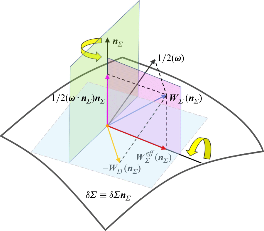
Rotation of a material surface element
 $\delta \boldsymbol{\varSigma }\equiv \delta {\varSigma }\boldsymbol{n}_{\varSigma }$
. Here
 $\boldsymbol{\omega }$
is the vorticity.
 $\boldsymbol{W}_{\varSigma }^{\textit{eff}}(\boldsymbol{n}_{\varSigma })$
and
 $\boldsymbol{W}_{\varSigma }(\boldsymbol{n}_{\varSigma })$
are the effective and total angular velocities of
 $\boldsymbol{n}_{\varSigma }$
, respectively;
 $-\boldsymbol{W}_{\kern-1.5pt D}(\boldsymbol{n}_{\varSigma })$
is the specific angular velocity of
 $\boldsymbol{n}_{\varSigma }$
. The yellow arrows indicate the rotation directions of
 $\boldsymbol{W}_{\varSigma }^{\textit{eff}}(\boldsymbol{n}_{\varSigma })$
and the gauge term
 $(\boldsymbol{\omega }\boldsymbol{\cdot }\boldsymbol{n}_{\varSigma })\boldsymbol{n}_{\varSigma }/2$
.

The physical quantities in (4.7) and (4.9) are illustrated in figure 2. Equation (4.9) indicates that a surface element undergoes the rigid rotation due to the combined effects of vorticity and strain rate, analogous to the interpretation for line-element rotation proposed by Corrsin & Karweit (Reference Corrsin and Karweit1972). However, the specific angular velocity of
 $\boldsymbol{n}_{\varSigma }$
is identified as
 $-\boldsymbol{W}_{\kern-1.5pt D}(\boldsymbol{n}_{\varSigma })$
, differing from that of a line element by a sign change. Since a fluid volume element contains material surface elements oriented in all possible directions, the surface average of
 $\boldsymbol{W}_{\kern-1.5pt D}(\boldsymbol{n}_{\varSigma })$
over all possible directions of
 $\boldsymbol{n}_{\varSigma }$
must vanish,
 \begin{eqnarray} \langle \boldsymbol{W}_{\kern-1.5pt D}(\boldsymbol{n}_{\varSigma })\rangle =\boldsymbol{0}, \end{eqnarray}
from which the first equality in (4.9) directly yields
 $\langle \boldsymbol{W}_{\varSigma }(\boldsymbol{n}_{\varSigma })\rangle ={1}/{2}\boldsymbol{\omega }$
. Subsequently, a comparison with (3.11) gives
 \begin{eqnarray} \boldsymbol{W}_{V}=\langle \boldsymbol{W}_{\varSigma }(\boldsymbol{n}_{\varSigma })\rangle =\frac {1}{2}\boldsymbol{\omega }, \end{eqnarray}
demonstrating that the angular velocity of a fluid volume element can be equivalently interpreted as the mean angular velocity of its constituent surface elements averaged over all possible spatial orientations. In addition, since
 $\boldsymbol{W}_{\kern-1.5pt D}(\boldsymbol{n}_{\varSigma })\perp \boldsymbol{n}_{\varSigma }$
, the first equality in (4.9) implies that
 $\boldsymbol{W}_{\varSigma }(\boldsymbol{n}_{\varSigma })\boldsymbol{\cdot }\boldsymbol{n}_{\varSigma }= {1}/{2}\boldsymbol{\omega }\boldsymbol{\cdot }\boldsymbol{n}_{\varSigma }$
which just coincides with the surface-normal component of the ‘mean angular velocity’
 $\boldsymbol{W}_{\textit{KB}}$
introduced by Batchelor (Reference Batchelor1967) and Thomson (Reference Thomson1869) (see Truesdell (Reference Truesdell1954)),
 \begin{eqnarray} \boldsymbol{W}_{\textit{KB}}\boldsymbol{\cdot }\boldsymbol{n}_{\varSigma }=\lim _{\epsilon \rightarrow 0}\frac {1}{2\pi \epsilon ^2}\oint _{C}\boldsymbol{u}\boldsymbol{\cdot }\, \text{d}\boldsymbol{r}=\frac {1}{2}\boldsymbol{\omega }\boldsymbol{\cdot }\boldsymbol{n}_{\varSigma }, \end{eqnarray}
for any open disk (with the radius
 $\epsilon$
) bounded by a circle
 $C$
centred at
 $\boldsymbol{x}$
and having the unit normal vector
 $\boldsymbol{n}_{\varSigma }$
. The condition
 $\boldsymbol{\omega }\boldsymbol{\cdot }\boldsymbol{n}_{\varSigma }=2\boldsymbol{W}_{\varSigma }(\boldsymbol{n}_{\varSigma })\boldsymbol{\cdot }\boldsymbol{n}_{\varSigma }$
is consistent with the case of a rotating rigid body immersed in a viscous flow, where the no-slip boundary condition is enforced on the solid surface.
From (4.6), we introduce the surface-element-based DVD,
 \begin{eqnarray} \boldsymbol{\omega }=\boldsymbol{R}_{\varSigma }(\boldsymbol{n}_{\varSigma })+\boldsymbol{s}_{\varSigma }(\boldsymbol{n}_{\varSigma })+\boldsymbol{g}_{\varSigma }(\boldsymbol{n}_{\varSigma }), \end{eqnarray}
where the vorticity constituents are given by
 \begin{align} \boldsymbol{R}_{\varSigma }(\boldsymbol{n}_{\varSigma }) & \equiv 2\boldsymbol{W}_{\varSigma }^{\textit{eff}}(\boldsymbol{n}_{\varSigma })=-2\boldsymbol{n}_{\varSigma }\times \left (\boldsymbol{A}\boldsymbol{\cdot }\boldsymbol{n}_{\varSigma }\right )=2\boldsymbol{n}_{\varSigma }\times \left (\boldsymbol{n}_{\varSigma }\boldsymbol{\cdot }\boldsymbol{B}\right ), \\[-9pt] \nonumber \end{align}
 \begin{align} \boldsymbol{s}_{\varSigma }(\boldsymbol{n}_{\varSigma }) & \equiv 2\boldsymbol{W}_{\kern-1.5pt D}(\boldsymbol{n}_{\varSigma })=2\boldsymbol{n}_{\varSigma }\times \left (\boldsymbol{D}\boldsymbol{\cdot }\boldsymbol{n}_{\varSigma }\right )=-2\boldsymbol{n}_{\varSigma }\times \left (\boldsymbol{n}_{\varSigma }\boldsymbol{\cdot }\boldsymbol{B}_{S}\right ), \\[-9pt] \nonumber \end{align}
 \begin{align} \boldsymbol{g}_{\varSigma }(\boldsymbol{n}_{\varSigma }) &\equiv \left (\boldsymbol{\omega }\boldsymbol{\cdot }\boldsymbol{n}_{\varSigma }\right )\boldsymbol{n}_{\varSigma }. \\[9pt] \nonumber \end{align}
In (4.14a
) and (4.14b
),
 $\boldsymbol{R}_{\varSigma }(\boldsymbol{n}_{\varSigma })$
and
 $\boldsymbol{s}_{\varSigma }(\boldsymbol{n}_{\varSigma })$
are termed the surface-element-based rigid-rotation and spin modes, respectively. Here
 $\boldsymbol{B}_{S}\equiv \vartheta \boldsymbol{I}-\boldsymbol{D}$
represents the symmetric part of
 $\boldsymbol{B}$
. As will be shown in § 6,
 $\boldsymbol{s}_{\varSigma }(\boldsymbol{n}_{\varSigma })$
is directly associated with the surface shear stress
 $\boldsymbol{\tau }$
. In (4.14c
),
 $\boldsymbol{g}_{\varSigma }(\boldsymbol{n}_{\varSigma })$
represents the surface-normal vorticity originating from the gauge term in (4.6). For a stationary solid boundary, the velocity adherence condition implies that the boundary vorticity is solely determined by the spin mode
 $\boldsymbol{s}_{\varSigma }(\boldsymbol{n}_{\varSigma })$
. It is worth noting that the streamsurface-based vorticity modes in (4.14) can be formally derived by making the following substitution in (3.13):
 \begin{eqnarray} \boldsymbol{e}\Rightarrow \boldsymbol{n}_{\varSigma },\ \boldsymbol{A}\Rightarrow \boldsymbol{B},\ \boldsymbol{D}\Rightarrow \boldsymbol{B}_{S}. \end{eqnarray}
5. Intrinsic relations for orthogonal line and surface elements
Consider a pair of orthogonal line and surface elements
 $ (\delta \boldsymbol{r},\delta \boldsymbol{\varSigma } )=(\delta {r}\boldsymbol{e},\delta \varSigma \boldsymbol{n}_{\varSigma })$
where
 $\boldsymbol{e}=\boldsymbol{n}_{\varSigma }$
holds at the considered instant. Since a volume element
 $\delta {V}$
is given by their dot product,
 $\delta {V}=\delta \boldsymbol{r}\boldsymbol{\cdot }\delta \boldsymbol{\varSigma }=\delta {r}\delta {\varSigma }$
, there must exist a kinematic relationship between the angular velocities of the line and surface elements. It is shown that the sum of (3.3a
) and (4.4a
) yields
 \begin{eqnarray} \frac {1}{\delta r}\frac {{\textrm D}\delta r}{{\textrm D}t}+ \frac {1}{\delta \varSigma }\frac {{\textrm D}\delta \varSigma }{{\textrm D}t}=\vartheta , \end{eqnarray}
which indicates that the dilatational motion of a volume element results from the superposition of the surface stretching motion and the normal extension. A general derivation of the rate of change of
 $\delta {V}$
is given in Appendix B.
Due to the presence of strain for fluid, neither
 $\boldsymbol{W}_{\varSigma }(\boldsymbol{n}_{\varSigma })$
nor
 $\boldsymbol{W}_{L}(\boldsymbol{n}_{\varSigma })$
equals
 ${1}/{2}\boldsymbol{\omega }$
individually (a condition satisfied only for rigid-body rotation), while each differs from
 ${1}/{2}\boldsymbol{\omega }$
by the specific angular velocity
 $\boldsymbol{W}_{\kern-1.5pt D}(\boldsymbol{n}_{\varSigma })$
. From the first equalities in (3.9) and (4.9), the sum and difference of
 $\boldsymbol{W}_{\varSigma }(\boldsymbol{n}_{\varSigma })$
and
 $\boldsymbol{W}_{L}(\boldsymbol{n}_{\varSigma })$
are given by
 \begin{align} \boldsymbol{W}_{\varSigma }(\boldsymbol{n}_{\varSigma })+\boldsymbol{W}_{L}(\boldsymbol{n}_{\varSigma }) & =\boldsymbol{\omega }, \\[-9pt] \nonumber \end{align}
 \begin{align} \boldsymbol{W}_{\varSigma }(\boldsymbol{n}_{\varSigma })-\boldsymbol{W}_{L}(\boldsymbol{n}_{\varSigma }) & =-\boldsymbol{s}_{\varSigma }(\boldsymbol{n}_{\varSigma })=-2\boldsymbol{W}_{\kern-1.5pt D}(\boldsymbol{n}_{\varSigma }). \\[9pt] \nonumber \end{align}
Equivalently, in terms of the vorticity modes, (5.2b ) can be expressed as
 \begin{eqnarray} \boldsymbol{R}_{L}(\boldsymbol{n}_{\varSigma })-\boldsymbol{R}_{\varSigma }(\boldsymbol{n}_{\varSigma })=2\boldsymbol{s}_{\varSigma }(\boldsymbol{n}_{\varSigma }). \end{eqnarray}
Equations (5.2a
) and (5.2b
) establish the general relations between the angular velocities of
 $ (\delta \boldsymbol{r},\delta \boldsymbol{\varSigma } )$
, revealing their complementary nature in both kinematics and geometry. First, combining (4.11) and (5.2a
) shows that the angular velocity of a fluid volume element is the arithmetic mean of those for
 $\delta \boldsymbol{r}$
and
 $\delta \boldsymbol{\varSigma }$
,
 \begin{eqnarray} \boldsymbol{W}_{V}=\frac {1}{2}\left [\boldsymbol{W}_{\varSigma }(\boldsymbol{n}_{\varSigma })+\boldsymbol{W}_{L}(\boldsymbol{n}_{\varSigma })\right ]. \end{eqnarray}
Second, (5.2b
) suggests that the surface-element-based spin mode is determined by the difference between the angular velocities of
 $\delta \boldsymbol{r}$
and
 $\delta \boldsymbol{\varSigma }$
. Taking the directional averages of both sides of (5.4) over all possible orientations of
 $\boldsymbol{n}_{\varSigma }$
recovers the previous result
 $\boldsymbol{W}_{V} = ({1}/{2})\boldsymbol{\omega }$
.
Taking the cross product of
 $\boldsymbol{n}_{\varSigma }$
with both sides of (5.2a
) yields
 \begin{eqnarray} \frac {{\textrm D}\boldsymbol{e}}{{\textrm D}t}+\frac {{\textrm D}\boldsymbol{n}_{\varSigma }}{{\textrm D}t}=\boldsymbol{\omega }\times \boldsymbol{n}_{\varSigma }. \end{eqnarray}
Then, the combination of (5.1) and (5.5) leads to
 \begin{eqnarray} \frac {1}{\delta \varSigma }\frac {{\textrm D}\delta \boldsymbol{\varSigma }}{{\textrm D}t} +\frac {1}{\delta {r}}\frac {{\textrm D}\delta \boldsymbol{r}}{{\textrm D}t}=\vartheta \boldsymbol{n}_{\varSigma }+\boldsymbol{\omega }\times \boldsymbol{n}_{\varSigma }, \end{eqnarray}
where the explicit dependence on
 $\boldsymbol{e}$
in the angular velocities has been formally eliminated. Equation (5.6) can alternatively be derived by summing (3.1) and (4.1), utilizing the relations
 $\boldsymbol{B}+\boldsymbol{A}=\vartheta \boldsymbol{I}+2\boldsymbol{\varOmega }$
and
 $2\boldsymbol{n}_{\varSigma }\boldsymbol{\cdot }\boldsymbol{\varOmega }=\boldsymbol{\omega }\times \boldsymbol{n}_{\varSigma }$
. We remark that (5.1)–(5.6) apply instantaneously to any orthogonal pair of material line and surface elements.
6. Physical interpretation of surface-element-based spin mode
Let us consider a material surface element
 $\delta \boldsymbol{\varSigma }\equiv \delta \varSigma \boldsymbol{n}_{\varSigma }$
. Building on the generalized decomposition of the VGT
 $\boldsymbol{A}\equiv \boldsymbol{\nabla }\boldsymbol{u}$
for arbitrarily moving and continuously deforming surfaces (Wu et al. Reference Wu, Yang, Luo and Pozrikidis2005), we express the VGT in a more convenient form,
 \begin{align} \boldsymbol{A}=\boldsymbol{n}_{\varSigma }\boldsymbol{n}_{\varSigma }\partial _{n}u_{n}+\boldsymbol{n}_{\varSigma }\left (\boldsymbol{\omega }_{r}\times \boldsymbol{n}_{\varSigma }\right )+\boldsymbol{n}_{\varSigma }\left (\boldsymbol{W}_{\varSigma }\times \boldsymbol{n}_{\varSigma }\right ) -\left (\boldsymbol{W}_{\varSigma }\times \boldsymbol{n}_{\varSigma }\right )\boldsymbol{n}_{\varSigma } +{\left (\boldsymbol{\nabla }_{\pi }\boldsymbol{u}\right )_{\pi }}, \end{align}
where
 $\boldsymbol{\omega }_{r}\equiv \boldsymbol{\omega }-2\boldsymbol{W}_{\varSigma }(\boldsymbol{n}_{\varSigma })$
represents the relative vorticity with
 $-2\boldsymbol{W}_{\varSigma }(\boldsymbol{n}_{\varSigma })$
accounting for the additional vorticity from the total angular velocity of rigid rotation of
 $\boldsymbol{n}_{\varSigma }$
. The condition (4.7) requires
 $\boldsymbol{\omega }_{r}$
to remain within the tangent space of
 $\delta \boldsymbol{\varSigma }$
. The decomposition in (6.1) reveals distinct physical interpretations for each component: the normal–normal (N–N) component is determined by
 $\partial _{n}u_{n}$
, representing the relative stretching rate normal to the surface; the normal–tangential (N–T) and tangential–normal (T–N) components are coupled to both the relative vorticity
 $\boldsymbol{\omega }_{r}$
and the angular velocity
 $\boldsymbol{W}_{\varSigma }(\boldsymbol{n}_{\varSigma })$
; the tangential–tangential (T–T) component is fully characterized by the surface velocity distribution, independent of off-surface velocity gradients.
The SAD of (6.1) yields the intrinsic decompositions of the strain-rate tensor
 $\boldsymbol{D}$
and vorticity tensor
 $\boldsymbol{\varOmega }$
,
 \begin{align} \boldsymbol{D} &=\boldsymbol{n}_{\varSigma }\boldsymbol{n}_{\varSigma }\partial _{n}u_{n}+\frac {1}{2}\boldsymbol{n}_{\varSigma }(\boldsymbol{\omega }_{r}\times \boldsymbol{n}_{\varSigma })+\frac {1}{2}(\boldsymbol{\omega }_{r}\times \boldsymbol{n}_{\varSigma })\boldsymbol{n}_{\varSigma }+{\mathscr{S}}[{\left (\boldsymbol{\nabla }_{\pi }\boldsymbol{u}\right )_{\pi }}], \\[-9pt] \nonumber \end{align}
 \begin{align} \boldsymbol{\varOmega } &=\frac {1}{2}\boldsymbol{n}_{\varSigma }(\boldsymbol{\omega }\times \boldsymbol{n}_{\varSigma })-\frac {1}{2}(\boldsymbol{\omega }\times \boldsymbol{n}_{\varSigma })\boldsymbol{n}_{\varSigma }+{\mathscr{A}}[{\left (\boldsymbol{\nabla }_{\pi }\boldsymbol{u}\right )_{\pi }}]. \\[9pt] \nonumber \end{align}
Equation (6.2a ) is the generalized Caswell formula (alternatively known as the Caswell–Wu formula), while (6.2b ) essentially realizes the orthogonal decomposition of vorticity in a tensorial form. Substituting (6.2a ) into (4.14b ) yields an elegant surface identity,
 \begin{eqnarray} \boldsymbol{s}_{\varSigma }(\boldsymbol{n}_{\varSigma })=2\boldsymbol{W}_{\kern-1.5pt D}(\boldsymbol{n}_{\varSigma })=\boldsymbol{\omega }_{r}, \end{eqnarray}
showing that the surface-element-based spin mode is identical to the relative vorticity. To our knowledge, this is an important result that has never been reported in prior literature. An immediate consequence of (6.3) is the universal expression for surface shear stress (exerted by the fluid at the
 $\boldsymbol{n}_{\varSigma }$
-side to the surface) in Newtonian fluids,
 \begin{eqnarray} \boldsymbol{\tau }=\mu \boldsymbol{\omega }_{r}\times \boldsymbol{n}_{\varSigma }=\mu \boldsymbol{s}_{\varSigma }(\boldsymbol{n}_{\varSigma })\times \boldsymbol{n}_{\varSigma }, \end{eqnarray}
with
 $\mu$
denoting the dynamic viscosity. An orthogonal surface-attached frame consists of a conjugate orthogonal pair
 $(\boldsymbol{\tau },\boldsymbol{\omega }_{r})$
and the unit normal vector
 $\boldsymbol{n}_{\varSigma }$
on a deformable surface, analogous to the
 $\boldsymbol{\tau }$
-frame (Wu et al. Reference Wu, Ma and Zhou2006) on a stationary solid boundary. For a material line element
 $\delta \boldsymbol{r}=\delta {r}\boldsymbol{e}$
with complementary surface element
 $\delta \boldsymbol{\varSigma }$
(where
 $\boldsymbol{n}_{\varSigma }=\boldsymbol{e}$
), we find the spin terms in (3.13b
) and (4.14b
) satisfy
 $\boldsymbol{s}_{L}(\boldsymbol{n}_{\varSigma })=-\boldsymbol{\omega }_{r}=-\boldsymbol{s}_{\varSigma }(\boldsymbol{n}_{\varSigma })$
, and the surface shear stress is
 $\boldsymbol{\tau }=\mu \boldsymbol{n}_{\varSigma }\times \boldsymbol{s}_{L}(\boldsymbol{n}_{\varSigma })$
. Therefore, the spin mode is alternatively termed the shear mode in viscous flows.
7. Streamline-based field description and vorticity decomposition
Historically, vortices have often been defined intuitively based on closed or spiralling streamlines. For instance, Robinson (Reference Robinson1991) proposed that a vortex exists when instantaneous streamlines projected onto a plane normal to the vortex core exhibit a roughly circular or spiral pattern in a reference frame moving with the vortex core centre. However, as Lugt (Reference Lugt1979) noted, streamlines lack Galilean and rotational invariance, meaning recirculatory streamline patterns at a certain instant in time do not necessarily reflect true vortex motions in which fluid particles rotate around a common axis. Consequently, a robust vortex identification method must satisfy Galilean invariance, keeping the vortex invariant under the choice of reference systems (Liu & Wang Reference Liu and Wang2020). Despite these limitations viewed from the algebraic perspective, the potential of streamline-based analysis within a field-theoretic framework remains underexplored. In particular, a systematic investigation into the interplay among streamlines, elementary vorticity modes and the rotational kinematics of directed material elements is still lacking.
In this section, we rigorously define the orbital rotation and spin modes of vorticity in terms of streamline geometry within a given reference frame, providing explicit vectorial expressions for each. These distinct modes are endowed with clear physical interpretations. Building on this foundation, we establish the relationship between the characteristic algebraic and field descriptions in §§ 9.5 and 9.6.
7.1. Streamline geometry and Frenet–Serret triad
In the field description, the counterpart of a material line element
 $\delta \boldsymbol{r}=\delta {r}\boldsymbol{e}$
is an infinitesimal streamline segment
 ${\mathcal{C}}$
, denoted as
 $\delta \bar {\boldsymbol{r}}=\delta {s}\boldsymbol{t}$
, where
 $s$
is the arclength parameter measured from a reference point on
 ${\mathcal{C}}$
, and
 $\delta {s}$
is its infinitesimal increment. At the considered instant,
 $\delta \bar {\boldsymbol{r}}$
coincides with
 $\delta \boldsymbol{r}$
. Each point on
 ${\mathcal{C}}$
is associated with an orthonormal right-handed triad
 $(\boldsymbol{t},\boldsymbol{n},\boldsymbol{b})$
, consisting of the unit tangent vector
 $\boldsymbol{t}$
, the principal normal vector
 $\boldsymbol{n}$
(pointing towards the streamline’s centre of curvature) and the binormal vector
 $\boldsymbol{b}\equiv \boldsymbol{t}\times \boldsymbol{n}$
(figure 3). The local curvature of
 ${\mathcal{C}}$
is denoted by
 $\kappa$
. The intrinsic evolution of
 $(\boldsymbol{t},\boldsymbol{n},\boldsymbol{b})$
along
 ${\mathcal{C}}$
is governed by the Frenet–Serret formulae from classical differential geometry (Serrin Reference Serrin1959; Chen Reference Chen2017). The osculating plane (spanned by
 $\boldsymbol{t}$
and
 $\boldsymbol{n}$
) and the normal plane (spanned by
 $\boldsymbol{n}$
and
 $\boldsymbol{b}$
) define the local geometry of
 ${\mathcal{C}}$
. Note that
 $\boldsymbol{n}$
is generally different from the unit normal vector
 $\boldsymbol{n}_{\varSigma }$
of an oriented surface. The velocity field along
 ${\mathcal{C}}$
is purely tangential and given by
 $\boldsymbol{u}=q\boldsymbol{t}$
, where
 $q\equiv \boldsymbol{u}\boldsymbol{\cdot }\boldsymbol{t}=\lVert \boldsymbol{u}\rVert$
is the velocity magnitude.
 $\partial _{s}\equiv \partial /\partial s$
represents the partial derivative with respect to
 $s$
for a physical quantity.
Schematic of the Frenet–Serret triad
 $(\boldsymbol{t},\boldsymbol{n},\boldsymbol{b})$
intrinsic to a regular streamline segment
 ${\mathcal{C}}$
with the local curvature radius
 $r_{0}\equiv \kappa ^{-1}$
. The streamline-based vorticity modes are shown as
 $(\boldsymbol{R}_{L}(\boldsymbol{t}),\boldsymbol{s}_{L}(\boldsymbol{t}),\boldsymbol{g}_{L}(\boldsymbol{t}))$
.

7.2. Streamline-based orbital-rotation mode
For a frozen velocity field, we observe that an orbital rotation along a streamline (segment)
 ${\mathcal{C}}$
occurs if and only if
 $\boldsymbol{t}\times \partial _{s}\boldsymbol{u}\neq \boldsymbol{0}$
(the non-collinearity between the tangent vector and the velocity variation in the osculating plane). Indeed, using the Frenet–Serret formula
 $\partial _{s}\boldsymbol{t}=\kappa \boldsymbol{n}$
and noting that
 $\boldsymbol{t}\times \boldsymbol{u}=\boldsymbol{0}$
, we find
 \begin{eqnarray} \boldsymbol{t}\times \partial _{s}\boldsymbol{u}=\kappa {q}\boldsymbol{b}, \end{eqnarray}
which indicates a local circular motion in the osculating plane about the binormal axis
 $\boldsymbol{b}$
. Thus, orbital rotation arises from streamline curvature
 $\kappa \neq {0}$
and non-zero speed
 $q\neq {0}$
. The radius of curvature is
 $r_{0}\equiv \kappa ^{-1}$
.
Since the directional derivative of velocity along a streamline can be expressed as
 $\partial _{s}\boldsymbol{u}=\boldsymbol{t}\boldsymbol{\cdot }\boldsymbol{A}$
, (7.1) can be adjusted to the form
 \begin{eqnarray} \boldsymbol{\psi }_{L}(\boldsymbol{t})\equiv \boldsymbol{t}\times \left (\boldsymbol{t}\boldsymbol{\cdot }\boldsymbol{A}\right )=\kappa {q}\boldsymbol{b}. \end{eqnarray}
We emphasize that in any flow field, the binormal vector
 $\boldsymbol{b}$
serves as the unique physically identifiable rotation axis external to the streamline orbit. Substituting
 $\boldsymbol{e} = \boldsymbol{t}$
into (3.4) yields the identity
 $\boldsymbol{W}_{L}^{\textit{eff}}(\boldsymbol{t}) = \boldsymbol{\psi }_{L}(\boldsymbol{t})$
. This reveals that
 $\boldsymbol{\psi }_{L}(\boldsymbol{t})$
in (7.2) can be interpreted as the effective angular velocity of
 $\boldsymbol{e}$
for a material line element instantaneously aligned with
 ${\mathcal{C}}$
(i.e.
 $\boldsymbol{e} = \boldsymbol{t}$
). Then, the vorticity in a reference rigid body (frozen with
 $\boldsymbol{t}$
) rotating with the angular velocity
 $\boldsymbol{\psi }_{L}(\boldsymbol{t})$
must be (figure 3)
 \begin{eqnarray} \boldsymbol{R}_{L}(\boldsymbol{t})=2\boldsymbol{t}\times \left (\boldsymbol{t}\boldsymbol{\cdot }\boldsymbol{A}\right )=2\kappa {q}\boldsymbol{b}. \end{eqnarray}
Here,
 $\boldsymbol{R}_{L}(\boldsymbol{t})$
is termed the streamline-based orbital-rotation mode (formally obtained from (3.13a
) via the substitution
 $\boldsymbol{e} = \boldsymbol{t}$
), analogous to a speed skater navigating a turn. Its binormal component is denoted by
 $R_{L}(\boldsymbol{t})\equiv \boldsymbol{R}_{L}(\boldsymbol{t})\boldsymbol{\cdot }\boldsymbol{b}=2\kappa {q}$
.
7.3. Streamline-based spin mode
Equation (7.3) immediately evokes a fundamental but often overlooked vorticity representation using the Frenet–Serret triad. This formulation appears in the classical literature (Serrin Reference Serrin1959, § 20) when expressed in the local rectangular coordinates aligned with
 $(\boldsymbol{t},\boldsymbol{n},\boldsymbol{b})$
,
 \begin{eqnarray} \boldsymbol{\omega }=\xi {q}\boldsymbol{t}+\partial _{b}q\boldsymbol{n}+\left (\kappa {q}-\partial _{n}q\right )\boldsymbol{b}, \end{eqnarray}
where the scalar factor
 $\xi$
,
 \begin{eqnarray} \xi \equiv \boldsymbol{t}\boldsymbol{\cdot }\left (\boldsymbol{\nabla }\times \boldsymbol{t}\right ) =\boldsymbol{b}\boldsymbol{\cdot }\partial _{n}\boldsymbol{t}-\boldsymbol{n}\boldsymbol{\cdot }\partial _{b}\boldsymbol{t}, \end{eqnarray}
was historically termed as the abnormality (also referred to as the torsion of the curve system or torsion of neighbouring vector lines). It was introduced as a measure of the departure of the velocity field from the property of having a normal congruence (Truesdell Reference Truesdell1954). The physical interpretation of this subtle parameter once perplexed prominent researchers, owing to the inherent limitation of the Frenet–Serret formalism: it applies to an individual curve but not to a family of neighbouring curves. However, the ambiguity is readily resolved by recognizing that
 $\xi {q}^{2}=\boldsymbol{\omega }\boldsymbol{\cdot }\boldsymbol{u}\equiv {h}$
represents the helicity density, implying
 $\xi =h/q^2$
(the ratio of helicity density to twice the kinetic energy density). In contrast to Serrin’s classical derivation, we can straightforwardly express the vorticity as
 $\boldsymbol{\omega }=\boldsymbol{\nabla }\times (q\boldsymbol{t} )=q\boldsymbol{\nabla }\times \boldsymbol{t}+\boldsymbol{\nabla }q\times \boldsymbol{t}$
. The first term expands further using the Frenet–Serret relations,
 $q\boldsymbol{\nabla }\times \boldsymbol{t}=\xi {q}\boldsymbol{t}+\kappa {q}\boldsymbol{b}$
, and the second term captures the variation of
 $q$
along the principal normal and binormal directions,
 $\boldsymbol{\nabla }q\times \boldsymbol{t}=\boldsymbol{n}\partial _{b}q-\boldsymbol{b}\partial _{n}q$
, as appeared in (7.4).
Consider now the spin mode associated with a streamline segment
 ${\mathcal{C}}$
. Owing to (7.3), (7.4) does not directly provide a vorticity decomposition into orbital and spin modes in the field description. However, a minor modification yields the desired splitting. Let
 $r$
denote the radial coordinate measured from the curvature centre of a point on
 ${\mathcal{C}}$
. Since
 $\partial _{n}q=-\partial _{r}q$
, the binormal vorticity component
 $\omega _{b}\equiv \boldsymbol{\omega }\boldsymbol{\cdot }\boldsymbol{b}$
becomes
 \begin{eqnarray} \omega _{b}=\kappa {q}-{\partial }_{n}q=\frac {1}{r_0}\frac {\partial }{\partial r}\left (rq\right ). \end{eqnarray}
A naïve identification of
 $\partial _{r}q$
as the spin component along the binormal direction
 $(s_{L}(\boldsymbol{t})\equiv \boldsymbol{s}_{L}(\boldsymbol{t})\boldsymbol{\cdot }\boldsymbol{b})$
leads to a paradox. Consider freezing the fluid near point
 $P$
into a rigid body rotating with angular velocity
 $W$
, such that
 $q=Wr$
. Although
 $\omega _{b}=2W$
correctly matches the rigid-body rotation, this approach would erroneously yield
 $s_{L}(\boldsymbol{t})=W$
instead of
 $s_{L}(\boldsymbol{t})=0$
. The resolution lies in recognizing that the principal normal
 $\boldsymbol{n}$
itself rotates, making
 $\partial _{n}q$
alone no longer characterize spin. The correct spin component must account for this rotation by subtracting the orbital contribution,
 \begin{eqnarray} s_{L}(\boldsymbol{t})=-\partial _{n}q-\kappa {q}=r_{0}\frac {\partial }{\partial r}\left (\frac {q}{r}\right ), \end{eqnarray}
analogous to a figure skater’s quadruple jump characterized by the radial velocity gradient. Furthermore, observing that
 $q\boldsymbol{\nabla }q=\boldsymbol{A}\boldsymbol{\cdot }\boldsymbol{u}$
(namely,
 $\boldsymbol{\nabla }q=\boldsymbol{A}\boldsymbol{\cdot }\boldsymbol{t}$
) and (7.2), we need to define, in general, the streamline-based spin mode as (figure 3)
 \begin{eqnarray} \boldsymbol{s}_{L}(\boldsymbol{t})\equiv \boldsymbol{\nabla }q\times \boldsymbol{t}-\boldsymbol{\psi }_{L}(\boldsymbol{t})=-2\boldsymbol{t}\times \left (\boldsymbol{t}\boldsymbol{\cdot }\boldsymbol{D}\right ). \end{eqnarray}
Remarkably,
 $\boldsymbol{s}_{L}(\boldsymbol{t})$
in (7.8) exhibits identical mathematical structure to the spin vorticity term
 $\boldsymbol{s}_{L}(\boldsymbol{e})$
in (3.13b
) when the alignment condition
 $\boldsymbol{e}=\boldsymbol{t}$
is imposed. Expanding (7.8) gives
 $\boldsymbol{s}_{L}(\boldsymbol{t})=\partial _{b}q\boldsymbol{n}+ (-\partial _{n}q-\kappa {q} )\boldsymbol{b}$
.
7.4. Streamline-based DVD
Based on the above discussion, we obtain the streamline-based DVD,
 \begin{eqnarray} \boldsymbol{\omega }=\boldsymbol{R}_{L}(\boldsymbol{t})+\boldsymbol{s}_{L}(\boldsymbol{t})+\boldsymbol{g}_{L}(\boldsymbol{t}), \end{eqnarray}
where the streamline-line orbital-rotation mode
 $\boldsymbol{R}_{L}(\boldsymbol{t})$
and spin mode
 $\boldsymbol{s}_{L}(\boldsymbol{t})$
are given in (7.3) and (7.8), respectively. The streamline-based streaming mode
 $\boldsymbol{g}_{L}(\boldsymbol{t})$
is defined as the streamline-parallel component (figure 3),
 \begin{eqnarray} \boldsymbol{g}_{L}(\boldsymbol{t})\equiv \left (\boldsymbol{\omega }\boldsymbol{\cdot }\boldsymbol{t}\right )\boldsymbol{t}=\xi {q}\boldsymbol{t}. \end{eqnarray}
We remark that (7.9) can also be derived from the Lamb decomposition of the convective acceleration,
 $\boldsymbol{u}\boldsymbol{\cdot }\boldsymbol{\nabla }\boldsymbol{u}=\boldsymbol{\omega }\times \boldsymbol{u}+\boldsymbol{\nabla }(q^{2}/2)$
, where
 $\boldsymbol{\omega }\times \boldsymbol{u}$
is the Lamb vector. Taking the cross product of
 $\boldsymbol{u}$
with both sides of this identity and employing the identity
 $\boldsymbol{\nabla }q = \boldsymbol{A} \boldsymbol{\cdot }\boldsymbol{t}$
yields the desired result.
8. Streamsurface-based field description and vorticity decomposition
8.1. Streamsurface-based DVD
Consider a material surface element
 $\delta \boldsymbol{\varSigma }\equiv \delta \varSigma \boldsymbol{n}_{\varSigma }$
instantaneously coinciding with an infinitesimal streamsurface element
 $\delta \overline {\boldsymbol{\varSigma }}\equiv \delta {S}\boldsymbol{n}_{S}$
, where
 $\delta \varSigma =\delta {S}$
and
 $\boldsymbol{n}_{\varSigma }=\boldsymbol{n}_{S}$
. A streamsurface
 $\mathcal{S}$
is formed by the set of streamlines passing through a reference curve in the flow field. Locally, the surface can be parameterized by two independent parameters
 $(x_{1},x_{2})$
, with
 $x_{3}$
denoting the normal coordinate. The associated orthonormal basis
 $(\overline {\boldsymbol{e}}_{1},\overline {\boldsymbol{e}}_{2},\overline {\boldsymbol{e}}_{3})$
defines a surface-attached reference frame, where
 $\overline {\boldsymbol{e}}_{3}=\overline {\boldsymbol{e}}_{1}\times \overline {\boldsymbol{e}}_{2}=\boldsymbol{n}_{S}$
. The surface curvature tensor is given by
 $\boldsymbol{K}\equiv -\boldsymbol{\nabla }_{\pi }\boldsymbol{n}_{S}=K_{\alpha \beta }\overline {\boldsymbol{e}}_{\alpha }\overline {\boldsymbol{e}}_{\beta }\ (\alpha ,\beta =1,2)$
, where
 $K_{\alpha \beta }$
are the tensor components. For conciseness, the partial derivatives with respective to the arclength parameters
 $(s_{1},s_{2})$
of the coordinate curves are denoted by
 \begin{eqnarray} \partial _{\alpha }\equiv \frac {\partial }{\partial {s}_{\alpha }}=\frac {1}{h_{\alpha }}\frac {\partial }{\partial {x}_{\alpha }},\ \alpha =1,2, \end{eqnarray}
where
 $h_{\alpha }\equiv \sqrt {g_{\alpha \alpha }}$
are Lamé coefficients, and
 $g_{\alpha \alpha }$
are the covariant metric components of the surface. When
 $(\overline {\boldsymbol{e}}_{1},\overline {\boldsymbol{e}}_{2})$
coincide with the two principal directions
 $(\overline {\boldsymbol{e}}_{\xi },\overline {\boldsymbol{e}}_{\eta })$
of
 $\delta \overline {\boldsymbol{\varSigma }}$
, with
 $\overline {\boldsymbol{e}}_{3}=\overline {\boldsymbol{e}}_{\zeta }=\boldsymbol{n}_{S}$
, the non-zero components of
 $\boldsymbol{K}$
are
 $(K_{\xi \xi },K_{\eta \eta })=(\lambda _{\xi },\lambda _{\eta })$
, where
 $\lambda _{\xi }$
and
 $\lambda _{\eta }$
denote the principal curvatures of
 $\mathcal{S}$
. In this principal frame
 $(\overline {\boldsymbol{e}}_{\xi },\overline {\boldsymbol{e}}_{\eta },\overline {\boldsymbol{e}}_{\zeta })$
, the streamsurface property
 $u_{\zeta }=0$
yields the following vorticity components (see Appendix C):
 \begin{align} \omega _{\xi } & =-\partial _{\zeta }\widehat {u}_{\eta }+\lambda _{\eta }u_{\eta },\ \omega _{\eta }=\partial _{\zeta }\widehat {u}_{\xi }-\lambda _{\xi }u_{\xi }, \\[-9pt] \nonumber \end{align}
 \begin{align} \omega _{\zeta } & =\partial _{\xi }u_{\eta }-\partial _{\eta }u_{\xi }+\kappa _{g,\xi }u_{\xi }-\kappa _{g,\eta }u_{\eta }, \\[9pt] \nonumber \end{align}
where
 $\kappa _{g,\xi }$
and
 $\kappa _{g,\eta }$
are the geodesic curvatures of the coordinate curves on the streamsurface, solely determined by the covariant metric components.
Analogous to the material description in (4.13) and (4.14), the streamsurface-based DVD is expressed as
 \begin{eqnarray} \boldsymbol{\omega }=\boldsymbol{R}_{\varSigma }(\boldsymbol{n}_{S})+\boldsymbol{s}_{\varSigma }(\boldsymbol{n}_{S})+\boldsymbol{g}_{\varSigma }(\boldsymbol{n}_{S}). \end{eqnarray}
The last term in (8.4) is equal to
 ${\omega _{3}}\boldsymbol{n}_{S}$
being equivalent to
 $2*{\mathscr{A}}[{ (\boldsymbol{\nabla }_{\pi }\boldsymbol{u} )_{\pi }}]$
, where
 $*$
is the Hodge-star operator (see Appendix C). By (4.5) and (4.14a
), the streamsurface-based orbital-rotation mode is determined as
 \begin{eqnarray} \boldsymbol{R}_{\varSigma }(\boldsymbol{n}_{S})\equiv -2\boldsymbol{n}_{S}\times \left (\boldsymbol{A}\boldsymbol{\cdot }\boldsymbol{n}_{S}\right )=2\lambda _{\eta }u_{\eta }\overline {\boldsymbol{e}}_{\xi }-2\lambda _{\xi }u_{\xi }\overline {\boldsymbol{e}}_{\eta }, \end{eqnarray}
representing a superposition of two regular circular motions: one with curvature radius
 $R_{\xi }=\lvert \lambda _{\xi }\rvert ^{-1}$
, and the other with
 $R_{\eta }=\lvert \lambda _{\eta }\rvert ^{-1}$
. From (4.14b
) and (6.3), the streamsurface-based spin mode is
 \begin{eqnarray} \boldsymbol{s}_{\varSigma }(\boldsymbol{n}_{S})=2\boldsymbol{n}_{S}\times \left (\boldsymbol{D}\boldsymbol{\cdot }\boldsymbol{n}_{S}\right )=(-\partial _{\zeta }\widehat {u}_{\eta }-\lambda _{\eta }u_{\eta })\overline {\boldsymbol{e}}_{\xi }+(\partial _{\zeta }\widehat {u}_{\xi }+\lambda _{\xi }u_{\xi })\overline {\boldsymbol{e}}_{\eta }, \end{eqnarray}
where each component exhibits the same form as its counterpart in planar flow. The resulting surface shear stress
 $\boldsymbol{\tau }=\tau _{\xi }\overline {\boldsymbol{e}}_{\xi }+\tau _{\eta }\overline {\boldsymbol{e}}_{\eta }$
on
 $\mathcal{S}$
is
 \begin{eqnarray} \tau _{\xi }=\mu (\partial _{\zeta }\widehat {u}_{\xi }+\lambda _{\xi }u_{\xi }),\ \tau _{\eta }=\mu (\partial _{\zeta }\widehat {u}_{\eta }+\lambda _{\eta }u_{\eta }). \end{eqnarray}
8.2. Consistency between different vorticity decompositions for a cylindrical streamsurface
The vorticity decompositions based on streamline
 ${\mathcal{C}}$
and streamsurface
 ${\mathcal{S}}$
are established in § 7.4 and § 8.1, respectively. In this subsection, we show the consistency between these two vorticity decompositions for a cylindrical streamsurface
 ${\mathcal{S}}$
with
 ${\mathcal{C}}$
as its directrix. Consider a pair of material line elements,
 $(\delta \boldsymbol{r},\delta \boldsymbol{r}^{\prime })=(\delta {r}\boldsymbol{e},\delta {r}^{\prime }\boldsymbol{e}^{\prime })$
, with
 $(\boldsymbol{e},\boldsymbol{e}^{\prime })=(\boldsymbol{t},\boldsymbol{n})$
(figure 4). This line-element pair can equivalently be viewed as a pair of material surface elements
 $(\delta \boldsymbol{\varSigma },\delta \boldsymbol{\varSigma }^{\prime })\equiv (\delta \varSigma \boldsymbol{n}_{\varSigma },\delta \varSigma ^{\prime }\boldsymbol{n}_{\varSigma }^{\prime })$
coinciding with
 ${\mathcal{S}}$
, where
 $(\boldsymbol{n}_{\varSigma },\boldsymbol{n}_{\varSigma }^{\prime })=(\boldsymbol{n},\boldsymbol{t})$
. The surface curvature tensor of
 ${\mathcal{S}}$
is
 $\boldsymbol{K}\equiv -\boldsymbol{\nabla }_{\pi }\boldsymbol{n}_{S}={\kappa }\boldsymbol{tt}$
so that the principal curvatures of
 ${\mathcal{S}}$
reduce to
 $(\lambda _{\xi }, \lambda _{\eta })=(\kappa ,0)$
, where
 $\kappa$
is the curvature of the streamline
 ${\mathcal{C}}$
. Since
 $\boldsymbol{g}_{\varSigma }(\boldsymbol{n})$
vanishes, the analysis focuses exclusively on the orbital-rotation and spin modes.
Sketch of a cylindrical streamsurface
 $\mathcal{S}$
generated by extending a regular streamline
 ${\mathcal{C}}$
(lying in the
 $\overline {\boldsymbol{e}}_{\xi }$
-
 $\overline {\boldsymbol{e}}_{\zeta }$
plane) along its binormal direction. The Frenet–Serret triad
 $(\boldsymbol{t},\boldsymbol{n},\boldsymbol{b})$
is defined at each point
 $P$
on
 ${\mathcal{C}}$
. The streamsurface normal
 $\boldsymbol{n}_{S}$
coincides with the principal normal
 $\boldsymbol{n}$
of
 ${\mathcal{C}}$
, with associated curvature radius
 $\kappa ^{-1}$
. The surface-attached frame
 $(\overline {\boldsymbol{e}}_{\xi },\overline {\boldsymbol{e}}_{\eta },\overline {\boldsymbol{e}}_{\zeta })$
is oriented such that
 $(\overline {\boldsymbol{e}}_{\xi },\overline {\boldsymbol{e}}_{\eta })$
align with the principal directions of
 $\mathcal{S}$
. Here
 $(\delta \boldsymbol{r},\delta \boldsymbol{r}^{\prime })$
represents a pair of orthogonal material line elements, with
 $\delta \boldsymbol{r}$
instantaneously coinciding with
 ${\mathcal{C}}$
. They can be viewed as a surface-element pair
 $(\delta \boldsymbol{\varSigma },\delta \boldsymbol{\varSigma }^{\prime })$
with
 $\delta \boldsymbol{\varSigma }$
residing on
 $\mathcal{S}$
.

Given the velocity field
 $\boldsymbol{u}=q\boldsymbol{t}$
on
 ${\mathcal{C}}$
, the streamsurface-based orbital-rotation mode in (8.5) equals to the streamline-based orbital-rotation mode,
 \begin{eqnarray} \boldsymbol{R}_{\varSigma }(\boldsymbol{n})=-2\kappa {q}\overline {\boldsymbol{e}}_{\eta }=2\kappa {q}\boldsymbol{b}=\boldsymbol{R}_{L}(\boldsymbol{t}). \end{eqnarray}
Equation (8.8) implies that the binormal components of
 $\boldsymbol{W}_{L}(\boldsymbol{t})$
and
 $\boldsymbol{W}_{\varSigma }(\boldsymbol{n})$
satisfy
 \begin{eqnarray} {W}_{\varSigma }(\boldsymbol{n})={W}_{L}(\boldsymbol{t})=\boldsymbol{t}\boldsymbol{\cdot }\boldsymbol{A}\boldsymbol{\cdot }\boldsymbol{n}=\kappa {q}, \end{eqnarray}
demonstrating that
 $\delta \boldsymbol{r}$
and
 $\delta \boldsymbol{\varSigma }$
rotates with the identical angular velocity
 $\kappa {q}$
. As a counterpart to (8.9), a similar relation follows,
 \begin{eqnarray} {W}_{L}(\boldsymbol{n})={W}_{\varSigma }(\boldsymbol{t}) =-\boldsymbol{n}\boldsymbol{\cdot }\boldsymbol{A}\boldsymbol{\cdot }\boldsymbol{t}=-\partial _{\zeta }{q}, \end{eqnarray}
showing that
 $\delta \boldsymbol{r}^{\prime }$
and
 $\delta \boldsymbol{\varSigma }^{\prime }$
also rotate with the identical angular velocity
 $-\partial _{\zeta }q$
, where the square of the velocity magnitude is
 ${q}^2=\widehat {u}_{\xi }^{2}+\widehat {u}_{\zeta }^{2}$
in a small neighbourhood of
 ${\mathcal{C}}$
. The streamsurface-based spin mode in (8.6) is equal to the streamline-based spin mode,
 \begin{eqnarray} \boldsymbol{s}_{\varSigma }(\boldsymbol{n}) =(\partial _{\zeta }\widehat {u}_{\xi }+\kappa {u}_{\xi })\overline {\boldsymbol{e}}_{\eta } =(-\partial _{\zeta }q-\kappa {q})\boldsymbol{b}=\boldsymbol{s}_{L}(\boldsymbol{t}). \end{eqnarray}
The second equality in (8.11) is due to the validity of the relations
 $\partial _{\zeta }\widehat {u}_{\xi } = \partial _{\zeta }{q}$
and
 $u_{\xi } = q$
on the considered streamline
 ${\mathcal{C}}$
.
By substituting (8.9) and (8.10) into (8.11), we find that the spin mode can be expressed in terms of the angular velocities describing the rigid-rotation modes of the orthogonal line-element pair
 $(\delta \boldsymbol{r},\delta \boldsymbol{r}^{\prime })$
or surface-element pair
 $(\delta \boldsymbol{\varSigma },\delta \boldsymbol{\varSigma }^{\prime })$
,
 \begin{align} {s}_{L}(\boldsymbol{t}) & ={W}_{L}(\boldsymbol{n})-{W}_{L}(\boldsymbol{t})={W}_{\varSigma }(\boldsymbol{t})-{W}_{\varSigma }(\boldsymbol{n}), \\[-9pt] \nonumber \end{align}
 \begin{align} {s}_{L}(\boldsymbol{t}) & ={W}_{\varSigma }(\boldsymbol{t})-{W}_{L}(\boldsymbol{t}) ={W}_{L}(\boldsymbol{n})-{W}_{\varSigma }(\boldsymbol{n}). \\[9pt] \nonumber \end{align}
As time evolves, the angle
 $\varTheta$
between the two material line elements will not remain
 $\pi /2$
due to their unequal angular velocities. Equation (8.12a
) implies that the rate of change of
 $\varTheta$
at the instant is equal to
 $s_{L}(\boldsymbol{t})$
. Furthermore,
 ${W}_{L}(\boldsymbol{t})$
and
 ${W}_{L}(\boldsymbol{n})$
can be decomposed as
 \begin{eqnarray} {W}_{L}(\boldsymbol{t})=\frac {1}{2}{\omega }_{b}+{W}_{D}(\boldsymbol{t}),\ {W}_{L}(\boldsymbol{n})=\frac {1}{2}{\omega }_{b}+{W}_{D}(\boldsymbol{n}), \end{eqnarray}
where their specific contributions are given by
 \begin{eqnarray} {W}_{D}(\boldsymbol{t})=-{W}_{D}(\boldsymbol{n})=\boldsymbol{t}\boldsymbol{\cdot }\boldsymbol{D}\boldsymbol{\cdot }\boldsymbol{n}=\frac {1}{2}\left (\kappa {q}+\partial _{\zeta }q\right ). \end{eqnarray}
9. Physical roles of rotational invariants
This section discusses the fundamental relationships among the material, field and characteristic algebraic descriptions, highlighting the physical significance of the rotational invariants in understanding these connections.
9.1. Normal-nilpotent decomposition and rotational invariants
In the region where the discriminant
 $\Delta _{\textrm{3D}}\gt 0$
,
 $\boldsymbol{A}\equiv \boldsymbol{\nabla }\boldsymbol{u}$
has one real eigenvalue
 $\lambda _{r}$
and a pair of complex conjugate eigenvalues
 $(\lambda _{1,2}=\lambda _{\textit{cr}}\pm {\textrm{i}}\lambda _{\textit{ci}})$
, where
 $\chi \equiv \lambda _{\textit{cr}}$
and
 $\lambda _{\textit{ci}}(\gt 0)$
represent the real and imaginary parts, respectively. At a given point
 $P$
, the rotation axis is specified by the real eigenvector
 $\boldsymbol{e}_{3}$
of
 $\boldsymbol{A}$
, which is uniquely determined by imposing a constraint for the axial vorticity component
 ${\omega }_{3}\equiv \boldsymbol{\omega }\boldsymbol{\cdot }\boldsymbol{e}_{3}\gt 0$
. The eigenpair
 $(\lambda _{r},\boldsymbol{e}_{3})$
satisfies the equation
 $\boldsymbol{e}_{3}\boldsymbol{\cdot }\boldsymbol{A}=\lambda _{r}\boldsymbol{e}_{3}$
. The rotation-axis-normal plane
 ${\mathcal{P}}$
is then identified as a 2-D subspace orthogonal to
 $\boldsymbol{e}_{3}$
. According to the classical critical-point theory (Chong et al. Reference Chong, Perry and Cantwell1990), a complex conjugate eigenvalue pair indicates a closed or spiral streamline pattern appearing in a small neighbourhood of
 $P$
on
 ${\mathcal{P}}$
. Under a proper orthonormal basis
 $(\boldsymbol{e}_{1},\boldsymbol{e}_{2},\boldsymbol{e}_{3})$
where
 $\boldsymbol{e}_{1}$
and
 $\boldsymbol{e}_{2}$
span the plane
 ${\mathcal{P}}$
, by employing the Schur theorem (Schur Reference Schur1909),
 $\boldsymbol{A}$
can be expressed in a real Schur form (that is, as a block upper triangular matrix in the field of real numbers), yielding the NND (Li Reference Li2010; Liu et al. Reference Liu, Gao, Tian and Dong2018; Li Reference Li2024),
 \begin{align} \boldsymbol{A} &= \begin{bmatrix} \chi & \psi +\gamma & -\beta \\[4pt] -\psi & \chi &\alpha \\[4pt] 0& 0& \lambda _{r} \end{bmatrix} =\boldsymbol{N}+\boldsymbol{S}, \\[-9pt] \nonumber \end{align}
 \begin{align} \boldsymbol{N} &= \begin{bmatrix} \chi & \psi & 0\\[4pt] -\psi & \chi &0\\[4pt] 0& 0& \lambda _{r} \end{bmatrix},\quad \boldsymbol{S}= \begin{bmatrix} 0 & \gamma & -\beta \\[4pt] 0& 0&\alpha \\[4pt] 0& 0& 0 \end{bmatrix}, \\[9pt] \nonumber \end{align}
where
 $\boldsymbol{N}$
is a normal tensor, and
 $\boldsymbol{S}$
is a nilpotent tensor. For notational simplicity, the same mathematical notation is employed for both a tensor and its corresponding matrix throughout the paper. The orthonormal basis
 $(\boldsymbol{e}_1, \boldsymbol{e}_2, \boldsymbol{e}_3)$
, which serves as the fundamental basis for the NND, is referred to as the NND basis or the NND triad (figure 5). The diagonal elements
 $(\chi , \lambda _r)$
in
 $\boldsymbol{A}$
and
 $\boldsymbol{N}$
describe the relative stretching rates of the material line elements along the NND axes. The off-diagonal element
 $\psi$
in
 $\boldsymbol{A}$
and
 $\boldsymbol{N}$
represents the characteristic angular velocity associated with the rigid rotation about
 $\boldsymbol{e}_3$
within
 ${\mathcal{P}}$
. The remaining invariants
 $(\alpha ,\beta ,\gamma )$
in
 $\boldsymbol{A}$
and
 $\boldsymbol{S}$
characterize the rates of angular deformation in the three orthogonal planes spanned by the NND triad. The dilatation is given by
 $\vartheta \equiv \textrm {tr}(\boldsymbol{A})=\boldsymbol{\nabla }\boldsymbol{\cdot }\boldsymbol{u}=2\chi +\lambda _{r}=\textrm {tr}(\boldsymbol{N})$
, where
 $\textrm {tr}$
denotes the trace. For
 $\Delta _{\textrm{3D}}\leq 0$
,
 $\boldsymbol{A}$
retains a matrix form analogous to (9.1a
), though no longer being a real Schur form (Li Reference Li2024).
Schematic of the right-handed NND triad
 $(\boldsymbol{e}_{1},\boldsymbol{e}_{2},\boldsymbol{e}_{3})$
on the rotation-axis-normal plane
 ${\mathcal{P}}$
, showing the rotation axis
 $\boldsymbol{e}_{3}$
(grey arrow, defined by
 $\omega _{3}\gt 0$
) and a typical swirling streamline (blue curve) near a point
 $P$
.

Using (9.1a
), the matrices of
 $\boldsymbol{D}$
and
 $\boldsymbol{\varOmega }$
in (2.1) are obtained as
 \begin{eqnarray} \boldsymbol{D}= \begin{bmatrix} \chi &\dfrac {1}{2}\gamma & -\dfrac {1}{2}\beta \\[8pt] \dfrac {1}{2}\gamma & \chi &\dfrac {1}{2}\alpha \\[8pt] -\dfrac {1}{2}\beta & \dfrac {1}{2}\alpha & \lambda _{r} \end{bmatrix}, \quad \boldsymbol{\varOmega }= \begin{bmatrix} 0 &\psi +\dfrac {1}{2}\gamma & -\dfrac {1}{2}\beta \\[8pt] -\left (\psi +\dfrac {1}{2}\gamma \right ) & 0&\dfrac {1}{2}\alpha \\[8pt] \dfrac {1}{2}\beta & -\dfrac {1}{2}\alpha & 0 \end{bmatrix}. \end{eqnarray}
Then, the vorticity
 $\boldsymbol{\omega }$
is derived as the dual vector of
 $\boldsymbol{\varOmega }$
, which is decomposed as
 \begin{align} \boldsymbol{\omega } & =\boldsymbol{R}_{N}+\boldsymbol{s}_{N}, \\[-9pt] \nonumber \end{align}
 \begin{align} \boldsymbol{R}_{N}=2\psi \boldsymbol{e}_{3}, & \quad \boldsymbol{s}_{N}=\alpha \boldsymbol{e}_{1}+\beta \boldsymbol{e}_{2}+\gamma \boldsymbol{e}_{3}. \\[9pt] \nonumber \end{align}
Equations (9.3a
) and (9.3b
) are collectively referred to as the invariant vorticity decomposition (IVD). Here
 $\boldsymbol{R}_{N}$
is termed the characteristic rigid-rotation mode;
 $\boldsymbol{s}_{N}$
is termed the characteristic spin mode whose in-plane components satisfy
 $(\omega _{1},\omega _{2})=(\alpha ,\beta )$
. The invariant vorticity splitting occurs exclusively for
 $\omega _{3}$
,
 \begin{eqnarray} \omega _{3}=2\psi +\gamma . \end{eqnarray}
From (9.1a
) and (9.1b
), we obtain the line-element-based representations of
 $(\boldsymbol{R}_{N},\boldsymbol{s}_{N})$
,
 \begin{eqnarray} \boldsymbol{R}_{N}=3\langle \boldsymbol{e}\times \left (\boldsymbol{e}\boldsymbol{\cdot }\boldsymbol{N}\right )\rangle ,\quad \boldsymbol{s}_{N}=3\langle \boldsymbol{e}\times \left (\boldsymbol{e}\boldsymbol{\cdot }\boldsymbol{S}\right )\rangle . \end{eqnarray}
The orientation of a reference frame in three-dimensional (3-D) space requires three scalars, while the second-order tensor
 $\boldsymbol{A}$
possesses nine independent elements. Consequently,
 $\boldsymbol{A}$
can be fully characterized by six intrinsic, orientation-invariant scalars. A conventional choice for these invariants comprises the three eigenvalues of
 $\boldsymbol{D}$
and the three vorticity components projected onto the
 $\boldsymbol{D}$
eigensystem, or alternatively, through properly defined tensor contractions (Meneveau Reference Meneveau2011). The real Schur form in (9.1a
) introduces a new set of rotational invariants
 $(\chi , \lambda _r, \alpha , \beta , \gamma , \psi )$
for generic compressible flows. Since
 $(\gamma , \psi )$
are functionally dependent on
 $(\lambda _{\textit{ci}}, \omega _3)$
(§ 9.4), an equivalent invariant set is
 $(\chi ,\lambda _{r},\alpha ,\beta ,\lambda _{\textit{ci}},\omega _{3})$
. This set encapsulates the complete eigenvalue information of
 $\boldsymbol{A}$
via
 $(\chi , \lambda _{\textit{ci}}, \lambda _r)$
, and the three vorticity components
 $(\alpha ,\beta ,\omega _{3})$
under the NND triad.
9.2. Rotational invariants and the generalized Caswell formula
The generalized Caswell formula (6.2a
) serves as the foundation for identifying the contribution of the surface-element-based spin mode to the surface vorticity. We now examine three special material surface elements
 $\delta \boldsymbol{\varSigma }^{(i)}=\delta \varSigma ^{(i)}\boldsymbol{e}_{i}$
(
 $i=1,2,3$
), with the unit normal vectors successively aligned with each NND basis vector. The material line element along
 $\boldsymbol{e}_{i}$
at the instant is denoted by
 $\delta \boldsymbol{r}^{(i)}=\delta {r}^{(i)}\boldsymbol{e}_{i}$
. Under the NND triad, the intrinsic decompositions of
 $\boldsymbol{D}$
in (6.2a
) and
 $\boldsymbol{\varOmega }$
in (6.2b
) are expressed as follows:
for
 $\delta \boldsymbol{\varSigma }^{(1)}=\delta \varSigma ^{(1)}\boldsymbol{e}_{1}$
,
 \begin{align} \boldsymbol{D} &=\begin{bmatrix} \chi &0 &0\\[8pt] 0 & 0&0\\[8pt] 0& 0& 0 \end{bmatrix}+ \begin{bmatrix} 0 &\dfrac {1}{2}\gamma & -\dfrac {1}{2}\beta \\[8pt] \dfrac {1}{2}\gamma & 0&0\\[8pt] -\dfrac {1}{2}\beta &0&0 \end{bmatrix}+ \begin{bmatrix} 0 &0 &0\\[8pt] 0 & \chi &\dfrac {1}{2}\alpha \\[8pt] 0& \dfrac {1}{2}\alpha & \lambda _{r} \end{bmatrix}, \end{align}
 \begin{align} \boldsymbol{\varOmega } &=\begin{bmatrix} 0 &\dfrac {1}{2}\omega _{3} &-\dfrac {1}{2}\beta \\[8pt] -\dfrac {1}{2}\omega _{3} & 0&0\\[8pt] \dfrac {1}{2}\beta & 0& 0 \end{bmatrix}+ \begin{bmatrix} 0 &0 &0\\[8pt] 0& 0&\dfrac {1}{2}\alpha \\[8pt] 0&-\dfrac {1}{2}\alpha &0 \end{bmatrix}; \end{align}
for
 $\delta \boldsymbol{\varSigma }^{(2)}=\delta \varSigma ^{(2)}\boldsymbol{e}_{2}$
,
 \begin{align} \boldsymbol{D} &=\begin{bmatrix} 0 &0 &0\\[8pt] 0 &\chi &0\\[8pt] 0& 0& 0 \end{bmatrix}+ \begin{bmatrix} 0 &\dfrac {1}{2}\gamma & 0\\[8pt] \dfrac {1}{2}\gamma & 0&\dfrac {1}{2}\alpha \\[8pt] 0&\dfrac {1}{2}\alpha &0 \end{bmatrix}+ \begin{bmatrix} \chi &0 &-\dfrac {1}{2}\beta \\[8pt] 0 &0&0\\[8pt] -\dfrac {1}{2}\beta & 0& \lambda _{r} \end{bmatrix}, \end{align}
 \begin{align} \boldsymbol{\varOmega} & =\begin{bmatrix} 0 &\dfrac {1}{2}\omega _{3} &0\\[8pt] -\dfrac {1}{2}\omega _{3} & 0&\dfrac {1}{2}\alpha \\[8pt] 0& -\dfrac {1}{2}\alpha & 0 \end{bmatrix}+ \begin{bmatrix} 0 &0 &-\dfrac {1}{2}\beta \\[8pt] 0& 0&0\\[8pt] \dfrac {1}{2}\beta &0&0 \end{bmatrix}; \end{align}
for
 $\delta \boldsymbol{\varSigma }^{(3)}=\delta \varSigma ^{(3)}\boldsymbol{e}_{3}$
,
 \begin{align} \boldsymbol{D} &=\begin{bmatrix} 0 &0 &0\\[8pt] 0 &0&0\\[8pt] 0& 0&\lambda _{r} \end{bmatrix}+ \begin{bmatrix} 0 &0 & -\dfrac {1}{2}\beta \\[8pt] 0 & 0&\dfrac {1}{2}\alpha \\[8pt] -\dfrac {1}{2}\beta &\dfrac {1}{2}\alpha &0 \end{bmatrix}+ \begin{bmatrix} \chi &\dfrac {1}{2}\gamma &0\\[8pt] \dfrac {1}{2}\gamma & \chi &0\\[8pt] 0& 0& 0 \end{bmatrix}, \end{align}
 \begin{align} \boldsymbol{\varOmega} &=\begin{bmatrix} 0 &0 &-\dfrac {1}{2}\beta \\[8pt] 0 & 0&\dfrac {1}{2}\alpha \\[8pt] \dfrac {1}{2}\beta & -\dfrac {1}{2}\alpha & 0 \end{bmatrix}+ \begin{bmatrix} 0 &\dfrac {1}{2}\omega _{3} &0\\[8pt] -\dfrac {1}{2}\omega _{3}& 0&0\\[8pt] 0&0&0 \end{bmatrix}. \end{align}
On the right-hand side of (9.6a
), (9.6c
) and (9.6e
), the matrices (from left to right) represent the normal stretching component (N–N), the symmetric shear component
 ${\mathscr{S}}[\boldsymbol{n}_{\varSigma }(\boldsymbol{\omega }_{r}\times \boldsymbol{n}_{\varSigma })]$
(T–N and N–T) and the in-plane component
 ${\mathscr{S}}[{ (\boldsymbol{\nabla }_{\pi }\boldsymbol{u} )_{\pi }}]$
(T–T). The surface-element-based spin mode
 $\boldsymbol{s}_{\varSigma }(\boldsymbol{e}_{i})$
is solely determined by two spin components
 \begin{align} \boldsymbol{s}_{\varSigma }(\boldsymbol{e}_{1})&=\boldsymbol{\omega }_{r}^{(1)}=\beta \boldsymbol{e}_{2}+\gamma \boldsymbol{e}_{3}=-\boldsymbol{s}_{L}(\boldsymbol{e}_{1}), \\[-9pt] \nonumber \end{align}
 \begin{align} \boldsymbol{s}_{\varSigma }(\boldsymbol{e}_{2})&=\boldsymbol{\omega }_{r}^{(2)}=\alpha \boldsymbol{e}_{1}-\gamma \boldsymbol{e}_{3}=-\boldsymbol{s}_{L}(\boldsymbol{e}_{2}), \\[-9pt] \nonumber \end{align}
 \begin{align} \boldsymbol{s}_{\varSigma }(\boldsymbol{e}_{3})&=\boldsymbol{\omega }_{r}^{(3)}=-\alpha \boldsymbol{e}_{1}-\beta \boldsymbol{e}_{2}=-\boldsymbol{s}_{L}(\boldsymbol{e}_{3}). \\[9pt] \nonumber \end{align}
Notably, only one spin component enters the matrix of
 ${\mathscr{S}}[{ (\boldsymbol{\nabla }_{\pi }\boldsymbol{u} )_{\pi }}]$
which characterizes the surface flexibility of
 $\delta \boldsymbol{\varSigma }^{(i)}$
. While the tensor
 ${\mathscr{S}}[{ (\boldsymbol{\nabla }_{\pi }\boldsymbol{u} )_{\pi }}]$
must be incorporated in the Cauchy–Poisson constitutive relation for the viscous stress tensor, it plays no dynamic role in generating surface shear stress. Moreover, the right-hand side matrices in (9.6b
), (9.6d
) and (9.6f
) represent the skew-symmetric tensors,
 ${\mathscr{A}}[\boldsymbol{n}_{\varSigma }(\boldsymbol{\omega }\times \boldsymbol{n}_{\varSigma })]$
and
 ${\mathscr{A}}[{ (\boldsymbol{\nabla }_{\pi }\boldsymbol{u} )_{\pi }}]$
, which determine the tangential and normal vorticity components, respectively.
Furthermore, for each orthogonal pair
 $(\delta \boldsymbol{\varSigma }^{(i)},\delta \boldsymbol{r}^{(i)})$
, the corresponding streamline- and streamsurface-based rigid-rotation modes are derived as
 \begin{align} \boldsymbol{R}_{L}(\boldsymbol{e}_{1})&=2\beta \boldsymbol{e}_{2}+2(\psi +\gamma )\boldsymbol{e}_{3},\ \boldsymbol{R}_{\varSigma }(\boldsymbol{e}_{1})=2\psi \boldsymbol{e}_{3}, \\[-9pt] \nonumber \end{align}
 \begin{align} \boldsymbol{R}_{L}(\boldsymbol{e}_{2}) &=2\alpha \boldsymbol{e}_{1}+2\psi \boldsymbol{e}_{3},\ \boldsymbol{R}_{\varSigma }(\boldsymbol{e}_{2})=2(\psi +\gamma )\boldsymbol{e}_{3}, \\[-9pt] \nonumber \end{align}
 \begin{align} \boldsymbol{R}_{L}(\boldsymbol{e}_{3}) &=\boldsymbol{0},\ \boldsymbol{R}_{\varSigma }(\boldsymbol{e}_{3})=2\alpha \boldsymbol{e}_{1}+2\beta \boldsymbol{e}_{2}. \\[9pt] \nonumber \end{align}
Evidently, (9.7) and (9.8) satisfy the relation in (5.3). These relations demonstrate that the rigid-rotation modes derived from the analyses of material line and surface elements fundamentally differ from those in the characteristic description. The characteristic spin components can modify the rigid-rotation modes of both material line and surface elements. The material line element aligned with
 $\boldsymbol{e}_{3}$
exhibits no rigid-rotation mode, while the rigid-rotation mode of
 $\boldsymbol{e}_{3}$
-oriented material surface element is exclusively determined by the two characteristic spin components
 $(\alpha ,\beta )$
.
9.3. Rotational invariants and Helmholtz decomposition
The NND triad
 $\{\boldsymbol{e}_{1},\boldsymbol{e}_{2},\boldsymbol{e}_{3}\}$
defines a Cartesian coordinate system
 $\boldsymbol{x}=(x_{1},x_{2},x_{3})$
in a small neighbourhood of
 $P$
. According to the Helmholtz–Hodge theorem, a smooth velocity field admits a global decomposition into longitudinal and transverse parts (Wu et al. Reference Wu, Ma and Zhou2015)
 \begin{align} \boldsymbol{u}=\boldsymbol{\nabla }\varPhi +\boldsymbol{v},\quad \boldsymbol{\nabla }\boldsymbol{\cdot }\boldsymbol{v}=0,\quad \boldsymbol{\nabla }\times \boldsymbol{v}=\boldsymbol{\omega }, \end{align}
where
 $\varPhi$
is the velocity potential, and
 $\boldsymbol{v}$
is the transverse velocity. This decomposition is unique in either an unbounded domain, or a bounded domain where
 $\boldsymbol{v}$
is parallel to the boundary. Evaluating the spatial gradient of (9.9) gives
 \begin{align} \boldsymbol{A}\equiv \boldsymbol{\nabla }\boldsymbol{u}=\boldsymbol{\nabla \boldsymbol{\nabla }}\varPhi +\boldsymbol{\nabla }\boldsymbol{v}, \end{align}
where
 $\boldsymbol{\nabla \boldsymbol{\nabla }}\varPhi =\partial _{i}\partial _{j}\varPhi \boldsymbol{e}_{i}\boldsymbol{e}_{j}$
is the potential Hessian, and the
 $\boldsymbol{\nabla }\boldsymbol{v}=\partial _{i}v_{j}\boldsymbol{e}_{i}\boldsymbol{e}_{j}$
is the transverse velocity gradient. The dilatation and vorticity are
 $\vartheta =\boldsymbol{\nabla} ^{2}\varPhi =\textrm {tr}(\boldsymbol{\nabla \boldsymbol{\nabla }}\varPhi )$
and
 $\boldsymbol{\omega }=\boldsymbol{\nabla }\times \boldsymbol{v}$
, respectively. By comparing the matrix in (9.1a
) with (9.10),
 $(A_{31},A_{32})=\partial _{3}\boldsymbol{u}_{\pi }=\boldsymbol{0}$
implies two constraints
 \begin{align} \partial _{3}\partial _{1}\varPhi =-\partial _{3}v_{1},\quad \partial _{3}\partial _{2}\varPhi =-\partial _{3}v_{2}, \end{align}
where
 $\boldsymbol{u}_{\pi }=(u_{1},u_{2})$
is the in-plane velocity field. Actually, it can be shown that
 $\partial _{3}\boldsymbol{u}_{\pi }=[\boldsymbol{e}_{3}\times (\boldsymbol{e}_{3}\boldsymbol{\cdot }\boldsymbol{A})]\times \boldsymbol{e}_{3}=\boldsymbol{W}_{L}^{\textrm{eff}}(\boldsymbol{e}_{3})\times \boldsymbol{e}_{3}$
. Since the rotation axis
 $\boldsymbol{e}_{3}$
satisfies
 $\boldsymbol{e}_{3}\boldsymbol{\cdot }\boldsymbol{A}=\lambda _{r}\boldsymbol{e}_{3}$
, the material line element aligned with
 $\boldsymbol{e}_{3}$
exhibits no effective rigid rotation, which ensures the intrinsic real Schur form of
 $\boldsymbol{A}$
.
The other rotational invariants in (9.1a ) are expressed as
 \begin{align} \chi &=\partial _{1}^{2}\varPhi +\partial _{1}v_{1}=\partial _{2}^{2}\varPhi +\partial _{2}v_{2},\quad \lambda _{r}=\partial _{3}^{2}\varPhi +\partial _{3}v_{3}, \\[-9pt] \nonumber \end{align}
 \begin{align} \alpha &=\partial _{2}\partial _{3}\varPhi +\partial _{2}v_{3},\quad \beta =-\partial _{1}\partial _{3}\varPhi -\partial _{1}v_{3}, \\[-9pt] \nonumber \end{align}
 \begin{align} 2\psi &=-2\partial _{2}\partial _{1}\varPhi -2\partial _{2}v_{1},\quad \gamma =2\partial _{1}\partial _{2}\varPhi +\partial _{1}v_{2}+\partial _{2}v_{1}. \\[9pt] \nonumber \end{align}
Applying (9.11) to (9.12b ) isolates the purely transverse contributions as
 \begin{align} \alpha =\partial _{2}v_{3}-\partial _{3}v_{2}=\omega _{1},\quad \beta =\partial _{3}v_{1}-\partial _{1}v_{3}=\omega _{2}. \end{align}
Note that both
 $2\psi$
and
 $\gamma$
in (9.12c
) incorporate the contributions from the potential and transverse velocities. However, the potential contributions (i.e.
 $\pm \partial _{1}\partial _{2}\varPhi$
) show opposite signs in their expressions, which cancel upon summation to yield
 $\omega _{3}=\partial _{1}v_{2}-\partial _{2}v_{1}$
in (9.4). Moreover, applying the SAD (2.1a
) to (9.10) gives
 \begin{align} \boldsymbol{D}=\boldsymbol{\nabla \boldsymbol{\nabla }}\varPhi +{\mathscr{S}}[\boldsymbol{\nabla }\boldsymbol{v}],\quad \boldsymbol{\varOmega }={\mathscr{A}}[\boldsymbol{\nabla }\boldsymbol{v}]. \end{align}
Equation (9.14) shows that the potential Hessian
 $\boldsymbol{\nabla \boldsymbol{\nabla }}\varPhi$
only contributes to
 $\boldsymbol{D}$
, whose diagonal matrix elements
 $(\partial _{1}^{2}\varPhi ,\partial _{2}^{2}\varPhi ,\partial _{3}^{2}\varPhi )$
affect the relative stretching rates
 $(\chi ,\lambda _{r})$
in (9.12a
).
 $\boldsymbol{\varOmega }$
is solely determined by the transverse velocity
 $\boldsymbol{v}$
.
9.4. Two IVDs
At the considered point
 $P$
, by restricting
 $\boldsymbol{A}$
in (9.1a
) to the rotation-axis-normal plane
 ${\mathcal{P}}$
, we obtain the restricted 2-D VGT under the basis
 $(\boldsymbol{e}_{1},\boldsymbol{e}_{2})$
,
 \begin{eqnarray} \kern1.5pt \widehat {\kern-1.5pt \boldsymbol{A}} \equiv \begin{bmatrix} \boldsymbol{e}_{1}\boldsymbol{\cdot }\boldsymbol{A}\boldsymbol{\cdot }\boldsymbol{e}_{1}&\boldsymbol{e}_{1}\boldsymbol{\cdot }\boldsymbol{A}\boldsymbol{\cdot }\boldsymbol{e}_{2}\\ \boldsymbol{e}_{2}\boldsymbol{\cdot }\boldsymbol{A}\boldsymbol{\cdot }\boldsymbol{e}_{1} & \boldsymbol{e}_{2}\boldsymbol{\cdot }\boldsymbol{A}\boldsymbol{\cdot }\boldsymbol{e}_{2} \end{bmatrix} =\begin{bmatrix} \chi &\psi +\gamma \\ -\psi & \chi \end{bmatrix}, \end{eqnarray}
whose characteristic equation is expressed as
 \begin{eqnarray} p(\lambda )\equiv \lambda ^{2}-2\chi \lambda +\chi ^{2}+\psi (\psi +\gamma )=0, \end{eqnarray}
where
 $p(\lambda )$
is a polynomial of the variable
 $\lambda$
. The discriminant of
 $p(\lambda )$
is
 \begin{eqnarray} \varDelta =4\lambda _{\textit{ci}}^{2}=4\psi (\psi +\gamma )=\omega _{3}^{2}-\gamma ^2. \end{eqnarray}
Obviously, in the region
 $\varDelta \gt 0$
(i.e.
 $\omega _{3}\gt \lvert \gamma \rvert$
), the complex conjugate eigenvalue pair of
 $\kern1.5pt \widehat {\kern-1.5pt \boldsymbol{A}}$
is
 $\lambda _{1,2}=\lambda _{\textit{cr}}\pm \textrm {i}\lambda _{\textit{ci}}$
, being exactly the same as that of
 $\boldsymbol{A}$
. The dilatation of the parallel flow on
 ${\mathcal{P}}$
is given by
 $\widehat {\vartheta }\equiv \textrm {tr}(\kern1.5pt \widehat {\kern-1.5pt \boldsymbol{A}})=2\chi$
. From a mathematical perspective, either
 $\gamma \gt 0$
(denoted as
 $\gamma ^{+}$
) or
 $\gamma \lt 0$
(denoted as
 $\gamma ^{-}$
) may serve as an alternative uniqueness condition for determining the real Schur form of
 $\boldsymbol{A}$
. The degenerate case with
 $\gamma =0$
implies
 $\omega _{3}=2\psi$
, representing purely the characteristic rigid rotation on
 ${\mathcal{P}}$
. To the best of our knowledge, this fundamental problem has not been explicitly analysed in the existing literature. As discussed below, this will yield two distinct IVDs corresponding to Case I and Case II, respectively.
(Case I) When
 $\gamma \gt 0$
, the condition
 $\omega _3 \gt \gamma \gt 0$
implies
 $\psi \gt 0$
. Let
 $(\psi ^+, \gamma ^+)$
denote the corresponding invariants and
 $(\boldsymbol{e}_{1}^{+},\boldsymbol{e}_{2}^{+},\boldsymbol{e}_{3}^{+})$
the associated NND triad (with
 $\boldsymbol{e}_{3}^{+}=\boldsymbol{e}_{3}$
). The first IVD is then established as
 \begin{align} \omega _{3}&=2\psi ^{+}+\gamma ^{+}, \\[-9pt] \nonumber \end{align}
 \begin{align} R_{N}^{+}\equiv 2\psi ^{+}&=\omega _{3}-\sqrt {\omega _{3}^{2}-4\lambda _{\textit{ci}}^{2}},\quad {s}_{N}^{+}\equiv \gamma ^{+}=\sqrt {\omega _{3}^{2}-4\lambda _{\textit{ci}}^{2}}. \\[9pt] \nonumber \end{align}
Equation (9.18a
) is essentially the Liutex-shear decomposition proposed by Liu et al. (Reference Liu, Gao, Tian and Dong2018). The characteristic rigid-rotation mode
 $\boldsymbol{R}_{N}^{+}\equiv 2\psi ^{+}\boldsymbol{e}_{3}$
is precisely the Liutex (or Rortex) vector introduced by Liu et al. (Reference Liu, Gao, Tian and Dong2018), which has been widely used to extract vortex in complex flows. The explicit expressions in (9.18b
) has previously been reported in studies such as Xu et al. (Reference Xu, Gao, Deng, Liu and Liu2019), Liu & Wang (Reference Liu and Wang2020) and more recently reviewed by Mao et al. (Reference Mao, Li, Yao and Wu2023). This case coincides with the KKB mechanism (§ 1): axial vortices form via the wrapping of shear layers, accompanied by a transfer from spin mode to rigid-rotation mode, ultimately resulting in vortex intensification.
(Case II) When
 $\gamma \lt 0$
, there is
 $2\psi \gt \omega _{3}\gt -\gamma \gt 0$
, which implies
 $\psi \gt -\gamma \gt 0$
. Let
 $(\psi ^{-},\gamma ^{-})$
denote the corresponding invariants and
 $(\boldsymbol{e}_{1}^{-},\boldsymbol{e}_{2}^{-},\boldsymbol{e}_{3}^{-})$
the associated NND triad (where
 $\boldsymbol{e}_{3}^{-}=\boldsymbol{e}_{3}$
). The second IVD is then established as
 \begin{align} \omega _{3}&=2\psi ^{-}+\gamma ^{-}, \\[-9pt] \nonumber \end{align}
 \begin{align} R_{N}^{-}\equiv 2\psi ^{-}&=\omega _{3}+\sqrt {\omega _{3}^{2}-4\lambda _{\textit{ci}}^{2}},\quad s_{N}^{-}\equiv \gamma ^{-}=-\sqrt {\omega _{3}^{2}-4\lambda _{\textit{ci}}^{2}}. \\[9pt] \nonumber \end{align}
In this case, the characteristic rigid-rotation mode is
 $\boldsymbol{R}_{N}^{-} \equiv 2\psi ^{-}\boldsymbol{e}_{3}$
. Equation (9.19a
) has been overlooked in the existing literature, primarily because
 $\gamma \gt 0$
is usually introduced as a uniqueness condition for determining the real Schur form of
 $\boldsymbol{A}$
. When the axial vortex has sufficient swirling strength to maintain its coherence, such that opposing spin effects cannot significantly disrupt the primary vortex structure, which we refer to as the anti-KKB mechanism/phenomenon. The physical validity of this case will be demonstrated through the Burgers vortex (§ 10.3) and the hurricane-eye structure on Saturn (§ 10.6).
From (9.18b ) and (9.19b ), the following identities are derived:
 \begin{eqnarray} \psi ^{+}=\psi ^{-}+\gamma ^{-},\quad \psi ^{-}=\psi ^{+}+\gamma ^{+},\quad \gamma ^{-}=-\gamma ^{+},\quad \omega _{3}=\psi ^{+}+\psi ^{-}. \end{eqnarray}
This leads to the concise representations for the discriminant
 $\varDelta$
and the imaginary part
 $\lambda _{\textit{ci}}$
:
 \begin{eqnarray} \varDelta =4\psi ^{+}\psi ^{-},\quad \lambda _{\textit{ci}}=\sqrt {\psi ^{+}\psi ^{-}}. \end{eqnarray}
Under the NND bases
 $(\boldsymbol{e}_{1}^{+},\boldsymbol{e}_{2}^{+})$
(Case I) and
 $(\boldsymbol{e}_{1}^{-},\boldsymbol{e}_{2}^{-})$
(Case II) on
 ${\mathcal{P}}$
, by using (9.15) and (9.20), the matrices of
 $\kern1.5pt \widehat {\kern-1.5pt \boldsymbol{A}}$
are, respectively, obtained as
 \begin{eqnarray} \text{Case I,}\ \kern1.5pt \widehat {\kern-1.5pt \boldsymbol{A}} =\begin{bmatrix} \chi &\psi ^{-}\\ -\psi ^{+} & \chi \end{bmatrix}; \quad \text{Case II,}\ \kern1.5pt \widehat {\kern-1.5pt \boldsymbol{A}} =\begin{bmatrix} \chi &\psi ^{+}\\ -\psi ^{-} & \chi \end{bmatrix}. \end{eqnarray}
We remark that
 $(\boldsymbol{e}_{1}^{+},\boldsymbol{e}_{2}^{+})$
can be obtained by rotating a given right-handed basis
 $(\boldsymbol{e}_{1}^{-},\boldsymbol{e}_{2}^{-})$
anticlockwise by an angle
 $\pi /2$
or
 $3\pi /2$
. Interestingly, we find that
 $\psi ^{+}$
and
 $\psi ^{-}$
are precisely the two eigenvalues of the matrix
 $\boldsymbol{Q}_{\theta }$
introduced by Nakayama (Reference Nakayama2017), which govern the azimuthal component of the relative velocity near the point
 $P$
,
 \begin{eqnarray} \widetilde {u}_{\theta }=(r\psi ^{+})\cos ^{2}\varTheta +(r\psi ^{-})\sin ^{2}\varTheta +O(r^2), \end{eqnarray}
where
 $r\gt 0$
is the radial distance from
 $P$
. To first order in
 $r$
, the minimum and maximum of
 $\widetilde {u}_{\theta }$
are
 $r\psi ^{+}$
and
 $r\psi ^{-}$
, respectively. Given that
 $\psi ^{+}\gt 0$
and
 $\psi ^{-}\gt 0$
, (9.23) demonstrates their combined role in establishing a unidirectional swirling motion around
 $P$
.
9.5. Relationship between characteristic and field descriptions
The streamline direction is a distinctive, physically significant direction. In the region where
 $\varDelta \gt 0$
, consider a regular streamline
 ${\mathcal{C}}$
passing through the point
 $P$
on the rotation-axis-normal plane
 ${\mathcal{P}}$
, equipped with the Frenet–Serret triad
 $(\boldsymbol{t},\boldsymbol{n},\boldsymbol{b})$
. The binormal vector aligns with the rotation axis
 $(\boldsymbol{b}=\boldsymbol{e}_{3})$
, giving
 $\omega _{b}=\omega _{3}\gt 0$
. Using (8.9) and (8.10), the matrix of
 $\kern1.5pt \widehat {\kern-1.5pt \boldsymbol{A}}$
in the streamline-attached basis
 $(\boldsymbol{t},\boldsymbol{n})$
is written as
 \begin{eqnarray} \kern1.5pt \widehat {\kern-1.5pt \boldsymbol{A}}_{\textrm{F-S}} \equiv \begin{bmatrix} \boldsymbol{t}\boldsymbol{\cdot }\boldsymbol{A}\boldsymbol{\cdot }\boldsymbol{t}&\boldsymbol{t}\boldsymbol{\cdot }\boldsymbol{A}\boldsymbol{\cdot }\boldsymbol{n}\\ \boldsymbol{n}\boldsymbol{\cdot }\boldsymbol{A}\boldsymbol{\cdot }\boldsymbol{t} & \boldsymbol{n}\boldsymbol{\cdot }\boldsymbol{A}\boldsymbol{\cdot }\boldsymbol{n} \end{bmatrix} =\begin{bmatrix} \chi (\boldsymbol{t}) &W_{L}(\boldsymbol{t})\\ -W_{L}(\boldsymbol{n}) & \chi (\boldsymbol{n}) \end{bmatrix}, \end{eqnarray}
where the relative stretching rates along
 $\boldsymbol{t}$
and
 $\boldsymbol{n}$
are
 \begin{eqnarray} \chi (\boldsymbol{t})\equiv \boldsymbol{t}\boldsymbol{\cdot }\boldsymbol{A}\boldsymbol{\cdot }\boldsymbol{t}=\boldsymbol{t}\boldsymbol{\cdot }\boldsymbol{D}\boldsymbol{\cdot }\boldsymbol{t},\quad \chi (\boldsymbol{n})\equiv \boldsymbol{n}\boldsymbol{\cdot }\boldsymbol{A}\boldsymbol{\cdot }\boldsymbol{n}=\boldsymbol{n}\boldsymbol{\cdot }\boldsymbol{D}\boldsymbol{\cdot }\boldsymbol{n}. \end{eqnarray}
Unlike in (9.15) and (9.22), the diagonal elements here are generally unequal:
 $\chi (\boldsymbol{t})\neq \chi (\boldsymbol{n})$
. The emergence of the irreducible real Schur form in (9.24) is particularly noteworthy, as it reveals the intrinsic structure of
 $\boldsymbol{A}$
through a streamline-based field description. Since (8.12a
) implies
 $W_{L}(\boldsymbol{n})=W_{L}(\boldsymbol{t})+s_{L}(\boldsymbol{t})$
, the matrix of
 $\kern1.5pt \widehat {\kern-1.5pt \boldsymbol{A}}$
under the basis
 $(-\boldsymbol{n},\boldsymbol{t})$
is given by
 \begin{eqnarray} \kern1.5pt \widehat {\kern-1.5pt \boldsymbol{A}}_{\textrm{F-S}} \equiv \begin{bmatrix} \boldsymbol{n}\boldsymbol{\cdot }\boldsymbol{A}\boldsymbol{\cdot }\boldsymbol{n}&-\boldsymbol{n}\boldsymbol{\cdot }\boldsymbol{A}\boldsymbol{\cdot }\boldsymbol{t}\\ -\boldsymbol{t}\boldsymbol{\cdot }\boldsymbol{A}\boldsymbol{\cdot }\boldsymbol{n} & \boldsymbol{t}\boldsymbol{\cdot }\boldsymbol{A}\boldsymbol{\cdot }\boldsymbol{t} \end{bmatrix} =\begin{bmatrix} \chi (\boldsymbol{n}) &W_{L}(\boldsymbol{t})+s_{L}(\boldsymbol{t})\\ -W_{L}(\boldsymbol{t}) & \chi (\boldsymbol{t}) \end{bmatrix}. \end{eqnarray}
The NND basis
 $(\boldsymbol{e}_{1}^{-},\boldsymbol{e}_{2}^{-})$
and the streamline basis
 $(\boldsymbol{t},\boldsymbol{n})$
are related through the following orthogonal transformation:
 \begin{eqnarray} \begin{bmatrix} \boldsymbol{t} & \boldsymbol{n} \end{bmatrix} =\begin{bmatrix} \boldsymbol{e}_{1}^{-} &\boldsymbol{e}_{2}^{-} \end{bmatrix} \begin{bmatrix} \cos \varTheta &-\sin \varTheta \\ \sin \varTheta & \cos \varTheta \end{bmatrix}, \end{eqnarray}
where
 $\varTheta$
is the azimuthal angle from the
 $\boldsymbol{e}_{1}^{-}$
axis. Combining (9.15), (9.20), (9.24) and (9.27) yields the following relations:
 \begin{align} & \chi (\boldsymbol{t})=\chi +\gamma ^{-}\sin \varTheta \cos \varTheta =\chi +\frac {1}{2}\gamma ^{-}\sin {2\varTheta }, \\[-9pt] \nonumber \end{align}
 \begin{align} & \chi (\boldsymbol{n})=\chi +\gamma ^{+}\sin \varTheta \cos \varTheta =\chi +\frac {1}{2}\gamma ^{+}\sin {2\varTheta }, \\[-9pt] \nonumber \end{align}
 \begin{align} & W_{L}(\boldsymbol{t})=\psi ^{-}+\gamma ^{-}\cos ^{2}\varTheta =\psi ^{+}\cos ^{2}\varTheta +\psi ^{-}\sin ^{2}\varTheta , \\[-9pt] \nonumber \end{align}
 \begin{align} & W_{L}(\boldsymbol{n})=\psi ^{-}+\gamma ^{-}\sin ^{2}\varTheta =\psi ^{-}\cos ^{2}\varTheta +\psi ^{+}\sin ^{2}\varTheta . \\[9pt] \nonumber \end{align}
Obviously, the upper and lower bounds of both
 $\chi (\boldsymbol{t})$
and
 $\chi (\boldsymbol{n})$
are
 $\chi + ({1}/{2})\gamma ^{+}$
and
 $\chi + ({1}/{2})\gamma ^{-}$
, respectively. The sum and difference of (9.28a
) and (9.28b
) give
 \begin{eqnarray} \chi (\boldsymbol{t})+\chi (\boldsymbol{n})=2\chi ,\quad \varphi (\boldsymbol{t})\equiv \chi (\boldsymbol{t})-\chi (\boldsymbol{n})=\gamma ^{-}\sin 2\varTheta . \end{eqnarray}
From (8.12a ), (9.28c ) and (9.28d ), it is implied that
 \begin{eqnarray} W_{L}(\boldsymbol{t})+W_{L}(\boldsymbol{n})=\omega _{3},\quad {s}_{L}(\boldsymbol{t})=\gamma ^{+}\cos 2\varTheta . \end{eqnarray}
Using (9.29) and (9.30), we obtain a concise relation for
 $(\gamma ^{\pm },s_{L}(\boldsymbol{t}),\varphi (\boldsymbol{t}))$
:
 \begin{eqnarray} \gamma ^{2}=s_{L}^{2}(\boldsymbol{t})+\varphi ^{2}(\boldsymbol{t}); \end{eqnarray}
and the angle
 $\varTheta$
must satisfy
 \begin{eqnarray} \tan 2\varTheta =-\frac {\varphi (\boldsymbol{t})}{s_{L}(\boldsymbol{t})}. \end{eqnarray}
We note that (9.31) reproduces the result reported by Chen & Liu (Reference Chen and Liu2025, (33a)). However, our derivation approach differs fundamentally from that used by Chen & Liu (Reference Chen and Liu2025) based on the frame-invariance of the discriminant
 $\varDelta$
for generic 2-D flows. The analysis in this subsection equally applies to a material line element
 $\delta \boldsymbol{r}\equiv \delta {r}\boldsymbol{e}$
on
 ${\mathcal{P}}$
, provided that the streamline-attached basis
 $(\boldsymbol{t},\boldsymbol{n})$
is replaced by
 $(\boldsymbol{e},\boldsymbol{e}_{\perp })$
where
 $\boldsymbol{e}_{\perp }\equiv \boldsymbol{e}_{3}\times \boldsymbol{e}$
.
9.6. Vorticity extrema
From (9.28c
) and (9.28d
), two fundamental equalities are derived for
 $({R}_{L}(\boldsymbol{t}),{s}_{L}(\boldsymbol{t}))$
:
 \begin{eqnarray} 2\psi ^{+}\leq {R}_{L}(\boldsymbol{t})\leq 2\psi ^{-},\quad \gamma ^{-}\leq {s}_{L}(\boldsymbol{t})\leq \gamma ^{+}. \end{eqnarray}
Equation (9.33) reveals that the streamline-based DVD vorticity modes
 $({R}_{L}(\boldsymbol{t}),{s}_{L}(\boldsymbol{t}))$
are rigorously bounded by the IVD vorticity modes
 $(2\psi ^{\pm },\gamma ^{\pm })$
. As illustrated in figure 6,
 $({R}_{L}(\boldsymbol{t}),{s}_{L}(\boldsymbol{t}))$
or
 $({R}_{L}(\boldsymbol{e}),{s}_{L}(\boldsymbol{e}))$
must reside along the principal diagonal of the square vorticity-mode space, bounded by the two critical configurations below.
-
(i) When
 $\boldsymbol{e}=\boldsymbol{e}_{2}^{+}$
or
$\boldsymbol{e}_{1}^{-}$
, the DVD vorticity modes correspond to the minimum rigid rotation
$2\psi ^{+}$
and the maximum spin
$\gamma ^{+}$
in Case I:(9.34)
\begin{align} R_{L}(\boldsymbol{e}_{2}^{+})=R_{L}(\boldsymbol{e}_{1}^{-})=2\psi ^{+},\quad s_{L}(\boldsymbol{e}_{2}^{+})=s_{L}(\boldsymbol{e}_{1}^{-})=\gamma ^{+}. \end{align}
-
(ii) When
$\boldsymbol{e}=\boldsymbol{e}_{1}^{+}$
or
$\boldsymbol{e}_{2}^{-}$
, the DVD vorticity modes correspond to the maximum rigid rotation
$2\psi ^{-}$
and the minimum spin
$\gamma ^{-}$
in Case II:(9.35)
\begin{align} R_{L}(\boldsymbol{e}_{1}^{+})=R_{L}(\boldsymbol{e}_{2}^{-})=2\psi ^{-},\quad s_{L}(\boldsymbol{e}_{1}^{+})=s_{L}(\boldsymbol{e}_{2}^{-})=\gamma ^{-}. \end{align}


From this perspective, the Liutex
 $\boldsymbol{R}_{N}^{+}\equiv 2\psi ^{+}\boldsymbol{e}_{3}$
(Liu et al. Reference Liu, Gao, Tian and Dong2018; Liu & Wang Reference Liu and Wang2020), widely used for vortex extraction, implicitly incorporates a minimization principle in its selection of the characteristic rigid-rotation mode.
The IVD and DVD actually provide complementary descriptions of vorticity kinematics at different levels for a generic flow field. The IVD modes (i.e. the vorticity extrema) can be evaluated to extract the primary features of flow structures at the characteristic algebraic level, albeit with some loss of flow details. In contrast, the DVD vorticity modes offer a more detailed description based on material and field perspectives, delivering deeper physical insight into the flow details. Therefore, a coupled IVD–DVD approach could enhance the physical understanding of the vorticity kinematics and structures, as demonstrated through several representative examples in § 10.
Illustration of the vorticity-mode diagram for the parallel flow in the rotation-axis-normal plane
 ${\mathcal{P}}$
. The DVD vorticity modes
 $(R_{L}(\boldsymbol{t}),s_{L}(\boldsymbol{t}))$
(represented by the cat symbol) are confined along the diagonal of the square domain of the vorticity-mode space, bounded by the IVD vorticity modes
 $(R_{N}^{\pm },s_{N}^{\pm })\equiv (2\psi ^{\pm },\gamma ^{\pm })$
(indicated by the yellow and red solid circles).

10. Examples
10.1. Simple shear flow and Joseph Bertrand’s puzzle
Consider a simple shear flow aligned with the Cartesian coordinate system
 $(x,y)$
, where
 $(\boldsymbol{e}_{x},\boldsymbol{e}_{y})$
denote the streamwise and vertical basis vectors, respectively. The velocity field
 $\boldsymbol{u}$
is prescribed as
 $(u_{x},u_{y})=(ky,0)\ (k\gt 0)$
. Hence, using the SAD in (2.1a
) and (2.1b
), the VGT
 $\boldsymbol{A}$
, the strain-rate tensor
 $\boldsymbol{D}$
, and the rotation-rate tensor
 $\boldsymbol{\varOmega }$
are evaluated as
 \begin{eqnarray} \boldsymbol{A}=k\boldsymbol{e}_{y}\boldsymbol{e}_{x},\quad \boldsymbol{D}=\frac {1}{2}(k\boldsymbol{e}_{x}\boldsymbol{e}_{y}+k\boldsymbol{e}_{y}\boldsymbol{e}_{x}),\quad \boldsymbol{\varOmega }=\frac {1}{2}(-k\boldsymbol{e}_{x}\boldsymbol{e}_{y}+k\boldsymbol{e}_{y}\boldsymbol{e}_{x}). \end{eqnarray}
The vorticity
 $\boldsymbol{\omega }$
is deduced as the dual vector of
 $\boldsymbol{\varOmega }$
, namely,
 $\boldsymbol{\omega }=-k\boldsymbol{e}_{z}$
. At the times of Helmholtz, Cauchy and Stokes, one could only apply the classical interpretation to postulate that a volume element of fluid must rotate with the angular velocity
 $\boldsymbol{W}_{V}=\boldsymbol{\omega }/2=-(k/2)\boldsymbol{e}_{z}$
. But then any material line element within a fluid volume element would obey the classical prediction, which however, fundamentally contradicts the truth that a material line element along
 $\boldsymbol{e}_{x}$
along the streamline direction shows no intuitive rotation. This precisely captures the essence of Joseph Bertrand’s famous puzzle in 1868: simple shear flow exhibits non-zero vorticity despite having entirely straight streamlines (Truesdell Reference Truesdell1954).
The
 $\boldsymbol{e}_{z}$
-components of (a)
 $(\boldsymbol{W}_{\kern-1.5pt D}(\boldsymbol{e}),\boldsymbol{W}_{L}(\boldsymbol{e}))$
and (b)
 $(\boldsymbol{R}_{L}(\boldsymbol{e}),\boldsymbol{s}_{L}(\boldsymbol{e}))$
for a material line element
 $\delta \boldsymbol{r}=\delta {r}\boldsymbol{e}$
, with the unit orientation vector
 $\boldsymbol{e}=\cos \theta \boldsymbol{e}_{x}+\sin \theta \boldsymbol{e}_{y}$
. The angle is normalized as
 $\theta ^* \equiv \theta /\pi$
. The angular velocities and vorticity components are normalized by
 $k/2$
and
 $k$
, respectively.

This paradox naturally disappears once the specific angular velocity
 $\boldsymbol{W}_{\kern-1.5pt D}(\boldsymbol{e})$
is recognized. For a material line element with
 $\boldsymbol{e}=\cos \theta \boldsymbol{e}_{x}+\sin \theta \boldsymbol{e}_{y}$
(
 $\theta$
is the angle from
 $\boldsymbol{e}_{x}$
), by using (3.7) and (3.9), we derive the specific and total angular velocities as
 \begin{align} & \boldsymbol{W}_{\kern-1.5pt D}(\boldsymbol{e})=\boldsymbol{e}\times (\boldsymbol{e}\boldsymbol{\cdot }\boldsymbol{D})=\frac {1}{2}k\cos 2\theta \boldsymbol{e}_{z}, \\[-9pt] \nonumber \end{align}
 \begin{align} & \boldsymbol{W}_{L}(\boldsymbol{e})=\boldsymbol{W}_{\kern-1.5pt D}(\boldsymbol{e})+\frac {1}{2}\boldsymbol{\omega }=\frac {1}{2}k(\cos 2\theta -1)\boldsymbol{e}_{z}. \\[9pt] \nonumber\end{align}
Correspondingly, the DVD vorticity modes are determined from (3.13a ) and (3.13b ) as
 \begin{eqnarray} \boldsymbol{R}_{L}(\boldsymbol{e})=k(\cos 2\theta -1)\boldsymbol{e}_{z},\quad \boldsymbol{s}_{L}(\boldsymbol{e})=-k\cos 2\theta \boldsymbol{e}_{z}. \end{eqnarray}
When
 $\boldsymbol{e}=\boldsymbol{e}_{x}=\boldsymbol{t}$
(
 $\theta =0$
) aligns with the streamline, the specific angular velocity
 $\boldsymbol{W}_{\kern-1.5pt D}(\boldsymbol{e}_{x})=(k/2)\boldsymbol{e}_{z}$
exactly cancels out
 $\boldsymbol{W}_{V}=-(k/2)\boldsymbol{e}_{z}$
, yielding
 $\boldsymbol{W}_{L}(\boldsymbol{e}_{x})=\boldsymbol{0}$
. The DVD modes are evaluated as
 $\boldsymbol{R}_{L}(\boldsymbol{t})=\boldsymbol{0}$
and
 $\boldsymbol{s}_{L}(\boldsymbol{t})=-k\boldsymbol{e}_{z}=\boldsymbol{\omega }$
. Hence, vorticity arises solely from the streamline-based spin mode, with no contribution from the orbital-rotation mode. Vorticity is not an appropriate physical measure to represent vortex in the spin-dominant region, despite a potentially high vorticity magnitude. Figures 7(a) and 7(b) display the
 $\boldsymbol{e}_{z}$
-components of
 $(\boldsymbol{W}_{\kern-1.5pt D}(\boldsymbol{e}),\boldsymbol{W}_{L}(\boldsymbol{e}))$
and
 $(\boldsymbol{R}_{L}(\boldsymbol{e}),\boldsymbol{s}_{L}(\boldsymbol{e}))$
, respectively. When
 $\theta$
increases from 0 to values within
 $(0,\pi /4)$
, both angular velocity components change:
 $0\lt W_{Dz}\lt k/2$
and
 $-k/2\lt W_{Lz}\lt 0$
, causing the clockwise rotation of the line element. At
 $\theta =\pi /4$
(i.e. the principal stretching axis of
 $\boldsymbol{D}$
), the specific angular velocity vanishes with
 $(W_{Dz},W_{Lz})=(0,-k/2)$
. Beyond this point
 $(\theta \in (\pi /4,3\pi /4))$
, the specific angular velocity component (dominated as
 $\cos 2\theta$
) becomes negative
 $(-k/2\leq {W}_{Dz}\lt 0)$
. The rotation continues until
 $\theta =3\pi /4$
(the principal compression axis of
 $\boldsymbol{D}$
), where
 $W_{Dz}$
again vanishes. Both components reach their minima at
 $\theta =\pi /2$
, with
 $(W_{Dz},W_{Lz})=(-k/2,-k)$
, while
 $W_{Lz}$
returns to zero at
 $\theta =\pi$
.
In the characteristic algebraic description, the condition
 $\omega _{3}\gt 0$
uniquely determines the rotation axis as
 $\boldsymbol{e}_{3}=-\boldsymbol{e}_{z}$
. From (10.4), the
 $\boldsymbol{e}_{3}$
-components of the line-element-based vorticity modes are
 $\overline {R}_{L}(\boldsymbol{e})=2k\sin ^{2}\theta$
and
 $\overline {s}_{L}(\boldsymbol{e})=k\cos 2\theta$
. For Case I ((9.18a
) and (9.18b
)), under the NND basis
 $(\boldsymbol{e}_{1}^{+},\boldsymbol{e}_{2}^{+})=(\boldsymbol{e}_{y},\boldsymbol{e}_{x})\ \text{or}\ (-\boldsymbol{e}_{y},-\boldsymbol{e}_{x})$
, the rotational invariants of
 $\boldsymbol{A}=k\boldsymbol{e}_{1}^{+}\boldsymbol{e}_{2}^{+}$
are given by
 $(2\psi ^{+},\gamma ^{+},\omega _{3})=(0,k,k)$
. Here
 $(\overline {R}_{L})_{\textit{min}}=2\psi ^{+}$
and
 $(\overline {s}_{L})_{\textit{max}}=\gamma ^{+}$
occur at
 $\theta =0$
(i.e.
 $\boldsymbol{e}=\boldsymbol{e}_{x}=\boldsymbol{t}$
) and
 $\pi$
(i.e.
 $\boldsymbol{e}=-\boldsymbol{e}_{x}$
). For Case II ((9.19a
) and (9.19b
)), under the NND basis
 $(\boldsymbol{e}_{1}^{-},\boldsymbol{e}_{2}^{-})=(\boldsymbol{e}_{x},-\boldsymbol{e}_{y})\ \text{or}\ (-\boldsymbol{e}_{x},\boldsymbol{e}_{y})$
, the rotational invariants of
 $\boldsymbol{A}=-k\boldsymbol{e}_{2}^{-}\boldsymbol{e}_{1}^{-}$
are given by
 $(2\psi ^{-},\gamma ^{-},\omega _{3})=(2k,-k,k)$
.
 $(\overline {R}_{L})_{\textit{max}}=2\psi ^{-}$
and
 $(\overline {s}_{L})_{\textit{min}}=\gamma ^{-}$
occur at
 $\theta =\pi /2$
(i.e.
 $\boldsymbol{e}=\boldsymbol{e}_{y}$
) and
 $3\pi /2$
(i.e.
 $\boldsymbol{e}=-\boldsymbol{e}_{y}$
). Physically, Case I corresponds to the rectilinear streamlines that exhibit no swirling motion, whereas Case II describes the behaviour of the material line elements oriented orthogonal to the streamline direction.
10.2. Potential flow outside a point vortex
For the pure potential flow
 $(\varDelta =-\gamma ^{2}\lt {0}\ \text{when}\ \gamma \neq {0})$
,
 $\boldsymbol{\omega }=\boldsymbol{0}$
implies
 $\alpha =\beta =0$
and
 $\gamma =-2\psi =2\partial _{1}\partial _{2}\varPhi$
. The characteristic spin component
 $\gamma$
coexists with the characteristic rigid-rotation component
 $\psi$
, which generates no surface shear stress due to the absence of viscosity. Consequently,
 $\boldsymbol{A}$
is fully described by three rotational invariants
 $(\chi ,\lambda _{r},\psi )$
where
 $\chi =\partial _{1}^{2}\varPhi =\partial _{2}^{2}\varPhi$
and
 $\lambda _{r}=\partial _{3}^{2}\varPhi$
(§ 9.3). The matrix of
 $\boldsymbol{A}$
in (9.1a
) is simplified as
 \begin{align} \boldsymbol{A}=\boldsymbol{D}=\boldsymbol{\nabla \boldsymbol{\nabla }}\varPhi = \begin{bmatrix} \chi & -\psi & 0\\[8pt] -\psi & \chi &0\\[8pt] 0& 0& \lambda _{r} \end{bmatrix} = \begin{bmatrix} \chi & \frac {1}{2}\gamma & 0\\[8pt] \frac {1}{2}\gamma & \chi &0\\[8pt] 0& 0& \lambda _{r} \end{bmatrix}. \end{align}
For a material line element
 $\delta \boldsymbol{r}=\delta {r}\boldsymbol{e}$
, (4.14) gives
 $\boldsymbol{R}(\boldsymbol{e})=-\boldsymbol{s}(\boldsymbol{e})=2\boldsymbol{e}\times (\boldsymbol{e}\boldsymbol{\cdot }\boldsymbol{\nabla \boldsymbol{\nabla }}\varPhi )$
.
Consider the potential flow outside a 2-D point vortex with the constant circulation
 $\varGamma =2\pi {K}\ (K\gt 0)$
. We adopt the cylindrical coordinate system
 $(r,\theta ,z)$
with the basis
 $(\boldsymbol{e}_{r},\boldsymbol{e}_{\theta },\boldsymbol{e}_{z})$
. For
 $r\gt 0$
, the azimuthal velocity component is
 $u_{\theta }(r)=K/r$
, and the VGT
 $\boldsymbol{A}$
is expressed as
 $\boldsymbol{A}=(\partial _{r}u_{\theta })\boldsymbol{e}_{r}\boldsymbol{e}_{\theta }-(u_{\theta }/r)\boldsymbol{e}_{\theta }\boldsymbol{e}_{r}$
. Under the NND triad
 $(\boldsymbol{e}_{1},\boldsymbol{e}_{2},\boldsymbol{e}_{3})=(\boldsymbol{e}_{r},\boldsymbol{e}_{\theta },\boldsymbol{e}_{z})$
, the invariants
 $(\psi ,\gamma ,\omega _{3})$
are given by (note
 $R_{N}=2\psi$
and
 $s_{N}=\gamma$
)
 \begin{eqnarray} \psi =\frac {u_{\theta }}{r}=\frac {K}{r^{2}},\quad \gamma =\frac {\partial {u}_{\theta }}{\partial r}-\frac {u_{\theta }}{r}=-\frac {2K}{r^{2}},\quad \omega _{3}=2\psi +\gamma =0. \end{eqnarray}
In contrast, the Liutex-based analysis (Liu et al. Reference Liu, Gao, Tian and Dong2018) yields
 $(\psi ,\gamma ,\omega _{3})=(0,0,0)$
in the region where
 $\varDelta \lt 0$
, which does not include the solution like (10.6).
To reveal the flow details, we examine the line-element-based DVD (in (3.12) and (3.13)) and the streamline-based DVD (in (7.3) and (7.8)). In this example, the Frenet–Serret frame of a circular streamline is just
 $(\boldsymbol{t},\boldsymbol{n},\boldsymbol{b})=(\boldsymbol{e}_{\theta },-\boldsymbol{e}_{r},\boldsymbol{e}_{z})$
. When
 $\boldsymbol{e}=\boldsymbol{t}=\boldsymbol{e}_{\theta }$
holds, we obtain
 \begin{eqnarray} \boldsymbol{R}_{L}(\boldsymbol{t})=2\frac {u_{\theta }}{r}\boldsymbol{e}_{z}=2\psi \boldsymbol{e}_{z}=\boldsymbol{R}_{N}, \quad \boldsymbol{s}_{L}(\boldsymbol{t})=\left (\frac {\partial u_{\theta }}{\partial r}-\frac {u_{\theta }}{r}\right )\boldsymbol{e}_{z}=\gamma \boldsymbol{e}_{z}=\boldsymbol{s}_{N}, \end{eqnarray}
where
 $(\boldsymbol{R}_{N},\boldsymbol{s}_{N})$
are the IVD vorticity modes in (9.3). When
 $\boldsymbol{e}=\boldsymbol{n}=-\boldsymbol{e}_{r}$
, we obtain
 \begin{align} & \boldsymbol{R}_{L}(\boldsymbol{n})=2\frac {\partial u_{\theta }}{\partial r}\boldsymbol{e}_{z}=2(\psi +\gamma )\boldsymbol{e}_{z}=-2\psi \boldsymbol{e}_{z}=-\boldsymbol{R}_{N}, \\[-9pt] \nonumber \end{align}
 \begin{align} & \boldsymbol{s}_{L}(\boldsymbol{n})=-\left (\frac {\partial u_{\theta }}{\partial r}-\frac {u_{\theta }}{r}\right )\boldsymbol{e}_{z}=-\gamma \boldsymbol{e}_{z}=-\boldsymbol{s}_{N}. \\[9pt] \nonumber \end{align}
10.3. Burgers vortex
The celebrated Burgers vortex is a steady, axisymmetric exact solution of the Navier–Stokes equations, widely used to model fine-scale turbulence structures owing to its finite and viscosity-independent total dissipation rate (Burgers Reference Burgers1948; Wu et al. Reference Wu, Ma and Zhou2015). It consists of an inward radial flow that concentrates and rotates around the symmetry axis, while the fluid moves outward in opposite directions along the axial dimension. In the following analysis, we adopt the cylindrical coordinate system
 $(r,\theta ,z)$
with the orthonormal basis
 $\{\boldsymbol{e}_{r},\boldsymbol{e}_{\theta },\boldsymbol{e}_{z}\}$
. The velocity field of the Burgers vortex is then expressed as
 \begin{align} & u_{r}=-\frac {1}{2}ar, \\[-9pt] \nonumber \end{align}
 \begin{align} & u_{\theta }=\frac {\varGamma }{2\pi r}\left [1-\exp \left (-\frac {r^2a}{4\nu }\right )\right ], \\[-9pt] \nonumber \end{align}
 \begin{align} & u_{z}=az. \\[9pt] \nonumber \end{align}
Here,
 $\varGamma$
denotes the total circulation that quantities the vortex strength; the positive constant
 $a$
represents the axial stretching rate,
 $\nu$
is the kinematic viscosity and
 $r$
is the radial distance measured from the
 $z$
-axis (i.e. the symmetry axis). For definiteness, we use the parameters (
 $a=0.084$
,
 $\varGamma =1.45$
,
 $\nu =0.01$
) reported in Shrestha et al. (Reference Shrestha, Nottage, Yu, Alvarez and Liu2021). Using (10.10), the matrices of
 $\boldsymbol{A}$
and
 $\boldsymbol{D}$
under
 $\{\boldsymbol{e}_{r},\boldsymbol{e}_{\theta },\boldsymbol{e}_{z}\}$
are given by
 \begin{eqnarray} \boldsymbol{A}= \begin{bmatrix} -\dfrac {1}{2}a &\dfrac {\partial u_{\theta }}{\partial r}& 0\\[8pt] -\dfrac {u_{\theta }}{r} &-\dfrac {1}{2}a&0\\[8pt] 0&0& a \end{bmatrix},\quad \boldsymbol{D}=\dfrac {1}{2} \begin{bmatrix} -a &\dfrac {\partial u_{\theta }}{\partial r}-\dfrac {u_{\theta }}{r}& 0\\[8pt] \dfrac {\partial u_{\theta }}{\partial r}-\dfrac {u_{\theta }}{r} &-a&0\\[8pt] 0&0& 2a \end{bmatrix}. \end{eqnarray}
Notably, the matrix
 $\boldsymbol{A}$
in (10.11) coincides precisely with the real Schur form in (9.1a
). Comparing (9.1a
) and
 $\boldsymbol{A}$
in (10.11) yields
 $(\chi ,\lambda _{r})=(-({1}/{2})a,a)$
and
 $(\alpha ,\beta )=(0,0)$
.
For Case II, the rotational invariants
 $(\psi ^{-},\gamma ^{-},\omega _{3})$
in (9.19a
) under the NND triad
 $\{\boldsymbol{e}_{1}^{-},\boldsymbol{e}_{2}^{-},\boldsymbol{e}_{3}^{-}\}=\{\boldsymbol{e}_{r},\boldsymbol{e}_{\theta },\boldsymbol{e}_{z}\}$
are given by
 \begin{align} & \psi ^{-}=\frac {u_{\theta }}{r},\quad R_{N}^{-}=2\psi ^{-}, \\[-9pt] \nonumber\end{align}
 \begin{align} & \gamma ^{-}=\frac {\partial {u}_{\theta }}{\partial r}-\frac {u_{\theta }}{r} =r\frac {\partial }{\partial r}\left (\frac {u_{\theta }}{r}\right ),\quad s_{N}^{-}=\gamma ^{-}, \\[-9pt] \nonumber\end{align}
 \begin{align} & \omega _{3}=2\psi ^{-}+\gamma ^{-}=\frac {\partial {u}_{\theta }}{\partial r}+\frac {u_{\theta }}{r} =\frac {1}{r}\frac {\partial }{\partial r}\left (ru_{\theta }\right ). \\[9pt] \nonumber\end{align}
Intuitively,
 $\psi ^{-}$
describes a virtual circular motion with speed
 $u_{\theta }$
and curvature radius
 $r$
. The corresponding characteristic rigid-rotation and spin modes are
 \begin{eqnarray} \boldsymbol{R}_{N}^{-}\equiv {R}_{N}^{-}\boldsymbol{e}_{3}^{-}=2\frac {{u}_{\theta }}{r}\boldsymbol{e}_{z},\quad \boldsymbol{s}_{N}^{-}\equiv {s}_{N}^{-}\boldsymbol{e}_{3}^{-}=r\frac {\partial }{\partial r}\left (\frac {u_{\theta }}{r}\right )\boldsymbol{e}_{z}. \end{eqnarray}
Substituting (10.10b ) into (10.12), we obtain the concrete expressions as
 \begin{align} & \psi ^{-}=\frac {\varGamma }{2\pi r^2}\left [1-\exp \left (-\frac {r^2a}{4\nu }\right )\right ], \\[-9pt] \nonumber\end{align}
 \begin{align} & \gamma ^{-}=\frac {\varGamma a}{4\pi \nu }\exp \left (-\frac {r^2a}{4\nu }\right )-\frac {\varGamma }{\pi r^2}\left [1-\exp \left (-\frac {r^2a}{4\nu }\right )\right ], \\[-9pt] \nonumber\end{align}
 \begin{align} & \omega _{3}=\frac {\varGamma a}{4\pi \nu }\exp \left (-\frac {r^2a}{4\nu }\right ). \\[9pt] \nonumber\end{align}
For Case I, the rotational invariants
 $(\psi ^{+},\gamma ^{+},\omega _{3})$
in (9.18b
) under the NND triad
 $\{\boldsymbol{e}_{1}^{+},\boldsymbol{e}_{2}^{+},\boldsymbol{e}_{3}^{+}\}=\left \{\boldsymbol{e}_{\theta },-\boldsymbol{e}_{r},\boldsymbol{e}_{z}\right \}$
are identified as
 \begin{align} \psi ^{+} & = \frac {\partial {u}_{\theta }}{\partial r},\quad R_{N}^{+}=2\psi ^{+}, \\[-9pt] \nonumber \end{align}
 \begin{align} \gamma ^{+} & = \frac {u_{\theta }}{r}-\frac {\partial {u}_{\theta }}{\partial r}=-r\frac {\partial }{\partial r}\left (\frac {u_{\theta }}{r}\right ),\quad s_{N}^{+}=\gamma ^{+}, \\[-9pt] \nonumber \end{align}
 \begin{align} \omega _{3} &= 2\psi ^{+}+\gamma ^{+}=\frac {\partial {u}_{\theta }}{\partial r}+\frac {u_{\theta }}{r}=\frac {1}{r}\frac {\partial }{\partial r}\left (ru_{\theta }\right ). \\[9pt] \nonumber \end{align}
Accordingly, the characteristic rigid-rotation and spin modes are given by
 \begin{eqnarray} \boldsymbol{R}_{N}^{+}\equiv {R}_{N}^{+}\boldsymbol{e}_{3}^{+}=2\frac {\partial {u}_{\theta }}{\partial r}\boldsymbol{e}_{z}, \quad \boldsymbol{s}_{N}^{+}\equiv {s}_{N}^{+}\boldsymbol{e}_{3}^{-}=-r\frac {\partial }{\partial r}\left (\frac {u_{\theta }}{r}\right )\boldsymbol{e}_{z}. \end{eqnarray}
For both cases, the discriminant
 $\varDelta$
in (9.17) admits a unified formulation:
 \begin{eqnarray} \varDelta =4\psi ^{+}\psi ^{-}=4\frac {u_{\theta }}{r}\frac {\partial {u}_{\theta }}{\partial r}. \end{eqnarray}
Unlike
 $\boldsymbol{R}_{N}^{-}$
in (10.13) governed by
 ${u_{\theta }}/{r}$
,
 $\boldsymbol{R}_{N}^{+}$
in (10.18) is just the Liutex vector associated with the radial velocity gradient
 $\partial _{r}u_{\theta }$
. This distinction renders
 $\boldsymbol{R}_{N}^{+}$
devoid of a kinematic interpretation via orbital rotation, due to its lack of a direct association with a specific orbit.
(a) Contour map of the normalized azimuthal velocity component
 $u_{\theta }$
with superposed streamlines for the Burgers vortex. (b) Radial profile of the normalized
 $u_{\theta }$
. (c) Comparison of the radial profiles of the normalized
 $\partial _{r}u_{\theta }$
,
 $u_{\theta }/r$
and the scaled discriminant
 $4\Delta$
.

The Burgers vortex emerges from a dynamic equilibrium among vorticity convection, vortex stretching and viscous diffusion. The reference scales for length, velocity and vorticity are thus introduced as
 $L_{\textit{ref}}\equiv ({\nu }/{a})^{1/2}$
,
 $U_{\textit{ref}}\equiv {\varGamma }/{L_{\textit{ref}}}$
and
 $\omega _{\textit{ref}}\equiv {\varGamma }/{L_{\textit{ref}}^2}$
, with an asterisk denoting normalized quantities. Figure 8(a) displays the distribution of the azimuthal velocity component
 $u_{\theta }^{*}$
on the rotation-axis-normal plane
 ${\mathcal{P}}$
, and its radial profile (along
 $y=0$
) is given in figure 8(b). The swirling streamlines indicate a 3-D vortex structure with axial stretching, because mass conservation requires outward axial flow to balance inward radial motion. We observe that
 $u_{\theta }$
exhibits a linear increase for small
 $r$
, following
 $u_{\theta }\sim {(\varGamma ar)}/{(8\pi \nu )}$
(or
 $u_{\theta }^{*}\sim {r^*}/{8\pi }$
in normalized form), matching the rigid-body rotation behaviour. It reaches a global maximum at the critical radius
 $r_{c}=r_{1}=2.242{L}_{\textit{ref}}$
(or
 $r_{c}^{*}=2.242$
), satisfying
 $\partial _{r}u_{\theta }(r_{c})=0$
. For
 $r\gt r_{c}$
, the velocity decays asymptotically as
 $u_{\theta }\sim {\varGamma }/{(2\pi r)}$
(or
 $u_{\theta }^{*}\sim {1}/{(2\pi {r}^*)}$
), showing characteristic of a potential vortex flow. Thus,
 $r_{c}$
naturally defines the vortex core radius. Figure 8(c) shows the radial distributions of
 $\partial _{r}u_{\theta }$
and
 ${u_{\theta }}/{r}$
, and the discriminant
 $\varDelta$
in (10.19), which govern the invariants in (10.12a
–
c
) and (10.17a
–
c
). As
 $r\rightarrow {0}$
, both
 $\partial _{r}u_{\theta }$
and
 ${u_{\theta }}/{r}$
approach
 ${\varGamma {a}}/{(8\pi \nu )}$
, confirming rigid-rotation characteristic within the vortex core. The quantity
 ${u_{\theta }}/{r}$
remains positive throughout and decays towards zero as
 $r\rightarrow {+\infty }$
, whereas
 $\partial _{r}u_{\theta }$
and
 $\varDelta$
reverse their signs at
 $r_c$
.
Contour maps of the normalized IVD variables for the Burgers vortex: (a)
 $2\psi ^{-}$
, (b)
 $\gamma ^{-}$
and (c)
 $\omega _{3}$
, with superposed streamlines. (d) Radial profiles of the normalized
 $2\psi ^{-}$
,
 $\gamma ^{-}$
,
 $\omega _{3}$
and the scaled discriminant
 $10\Delta$
.

Figure 9 presents the contour plots of the IVD variables
 $(2\psi ^{-},\gamma ^{-},\omega _{3})$
, with radial profiles shown in figure 9(d). The rigid-rotation mode
 $(R_{N}^{-}=2\psi ^{-})$
(figure 9
a) remains strictly positive and vanishes at infinity. In contrast, the spin mode
 $(s_{N}^{-}=\gamma ^{-})$
(figure 9
b) is exclusively negative, featuring a null point at the vortex-axis position
 $r_{\gamma }^{(1)}=0$
and a pronounced minimum at
 $r_{\gamma }^{(2)}$
(
 $r_{c}=r_{1}\lt r_{\gamma }^{(2)}\lt r_{2}$
), where
 $r_{2}$
is the inflection point of
 $u_{\theta }$
(
 $\partial _{r}^{2}u_{\theta }(r_2)=0$
). This minimum corresponds to the twin negative peaks in figure 9(d), revealing a dual-cored spin structure. The existence of
 $r_{\gamma }^{(2)}$
is qualitatively analysed as follows. At
 $r=r_{1}$
where
 $\partial _{r}u_{\theta }(r_{1})=0$
, figure 8(c) shows the negative slopes for both
 $\partial _{r}u_{\theta }$
and
 ${u_{\theta }}/{r}$
, with
 $\partial _{r}^{2}u_{\theta }(r_1)\lt \partial _{r}({u_{\theta }}/{r})(r_{1})$
, implying
 $\partial _{r}\gamma (r_{1})\lt 0$
. At
 $r=r_{2}$
, the slope reversal gives
 $\partial _{r}\gamma (r_{2})=-\partial _{r}({u_{\theta }}/{r})(r_{2})\gt 0$
. By the intermediate value theorem, there must exist a critical point
 $r_{\gamma }^{(2)}\in (r_{1},r_{2})$
of
 $\partial _{r}\gamma$
where
 $\gamma$
actually attains a minimum. The superposition of
 $2\psi ^{-}$
and
 $\gamma ^{-}$
produces the vorticity
 $\omega _z (=\omega _3)$
, with a more localized distribution than
 $2\psi ^{-}$
, as seen in both figures 9(c) and 9(d).
Note that for any fixed
 $z$
, a local comoving frame transformation
 $(\boldsymbol{u}\rightarrow \boldsymbol{u}-u_{z}(z)\boldsymbol{e}_{z})$
reduces the analysis to the rotation-axis-normal plane
 ${\mathcal{P}}$
which preserves all essential vortex kinematics. Since the in-plane velocity
 $\boldsymbol{u}_{\pi }(r,\theta )=u_{r}(r)\boldsymbol{e}_{r}+u_{\theta }(r)\boldsymbol{e}_{\theta }$
is independent of
 $z$
, we only need to analyse
 $z=0$
. Substituting (10.11) into (7.3) and (7.8) yields the streamline-based vorticity modes,
 \begin{align} & {R}_{L}(\boldsymbol{t})=2\psi ^{-}+2\frac {u_r^2}{q^2}\gamma ^{-}=2\psi ^{-}+2\gamma ^{-}\cos ^2{\varTheta }, \\[-12pt] \nonumber \end{align}
 \begin{align} & {s}_{L}(\boldsymbol{t})=\frac {u_{\theta }^{2}-u_{r}^{2}}{q^2}\gamma ^{-}=\gamma ^{+}\cos 2\varTheta , \\[9pt] \nonumber \end{align}
where
 $(\cos \varTheta ,\sin \varTheta )=(u_{r}/q,u_{\theta }/q)$
with
 $q^{2}=u_{\theta }^{2}+u_{r}^{2}$
and
 $\varTheta$
being the azimuthal angle from
 $\boldsymbol{e}_{r}$
. Equation (10.20a
) and (10.20b
) are consistent with the general theory in § 9.5.
Contour maps of the normalized streamline-based DVD vorticity modes on the rotation-axis-normal plane
 ${\mathcal{P}}$
for the Burgers vortex: (a)
 ${R}_{L}(\boldsymbol{t})$
and (b)
 ${s}_{L}(\boldsymbol{t})$
, with superposed streamlines. (c) Radial profiles of the normalized
 ${R}_{L}(\boldsymbol{t})$
,
 ${s}_{L}(\boldsymbol{t})$
,
 $\omega _{3}$
and the scaled discriminant
 $10\Delta$
.

Figure 10 presents the axial components of the DVD variables
 $({R}_{L}(\boldsymbol{t}),{s}_{L}(\boldsymbol{t}),{\omega }_{z})$
, with the radial distributions shown in figure 10(c). The DVD vorticity modes (figures 10
a and 10
b) resemble their IVD counterparts (figures 9
a and 9
b):
 ${R}_L(\boldsymbol{t})$
retains the monopole structure of
 $R_{N}^{-}$
, while
 ${s}_L(\boldsymbol{t})$
preserves the dipole character of
 $s_{N}^{-}$
(figures 9
d and 10
c). The radial distributions of
 $(R_{N}^{-},R_{N}^{+},{R}_{L}(\boldsymbol{t}))$
and
 $(s_{N}^{-},s_{N}^{+},s_L(\boldsymbol{t}))$
are compared in figures 11(a) and 11(b), respectively. Indeed, the DVD vorticity modes are always bounded by the IVD vorticity modes. In the vortex core
 $(r\lt {r_c},\Delta \gt 0)$
, since
 $u_{\theta }$
dominates the in-plane velocity field
 $(\lvert {u}_{\theta }\rvert \gg \lvert {u}_{r}\rvert )$
, (10.20a
) and (10.20b
) imply
 $R_{L}(\boldsymbol{t})\approx 2\psi ^{-}=R_{N}^{-}$
and
 $s_{L}(\boldsymbol{t})\approx \gamma ^{-}=s_{N}^{-}$
, which explain their close agreement. The deviation of
 $R_N^{+}$
from
 $R_L(\boldsymbol{t})$
is due to the term
 $2\gamma ^{+}\sin ^2\varTheta =2\gamma ^{+}(u_{\theta }/q)^2$
, as seen from the alternative expression based on the IVD vorticity modes
 $(R_{N}^{+},s_{N}^{+})$
in Case I:
 \begin{eqnarray} {R}_{L}(\boldsymbol{t})=2\psi ^{+}+2\frac {u_\theta ^2}{q^2}\gamma ^{+}=2\psi ^{+}+2\gamma ^{+}\sin ^2{\varTheta }. \end{eqnarray}
Both
 $R_{N}^{+}$
and
 $R_{N}^{-}$
converge to the same limit
 ${\varGamma a}/{(4\pi \nu )}$
as
 $r\rightarrow {0}$
. In the region
 $r^{*}\gt 5$
, the difference between
 $R_{N}^{-}$
and
 $R_{L}(\boldsymbol{t})$
is caused by
 $2\gamma ^{-}\cos ^{2}\varTheta =2\gamma ^{-}(u_{r}/q)^{2}$
in (10.20a
). According to (10.20b
), the sign reversal of
 $s_L(\boldsymbol{t})$
with increasing
 $r$
is attributed to the growing influence of the radial velocity magnitude
 $|u_r|$
.
Comparison of (a)
 $(R_{N}^{-},R_{N}^{+},{R}_{L}(\boldsymbol{t}))$
and (b)
 $(s_{N}^{-},s_{N}^{+},{s}_{L}(\boldsymbol{t}))$
for the Burgers vortex where
 $(R_{N}^{\pm },s_{N}^{\pm })=(2\psi ^{\pm },\gamma ^{\pm })$
. The discriminant
 $\varDelta$
has been multiplied by 5 and 3 in (a) and (b), respectively.

Furthermore, for a material line element on
 ${\mathcal{P}}$
with orientation
 $\boldsymbol{e}=\cos \hat {\varTheta }\boldsymbol{e}_{r}+\sin \hat {\varTheta }\boldsymbol{e}_{\theta }$
, the associated DVD vorticity modes are given by
 \begin{align} R_{L}(\boldsymbol{e})=2\psi ^{+}\cos ^{2}\hat {\varTheta }+2\psi ^{-}\sin ^{2}\hat {\varTheta },\quad s_{L}(\boldsymbol{e})=\gamma ^{+}\cos 2\hat {\varTheta }. \end{align}
Their extrema confirm the IVD modes as rigorous bounds, attained at specific orientations. Here
 $(R_{L})_{\textit{max}}=2\psi ^{-}$
and
 $(s_{L})_{\textit{min}}=\gamma ^{-}$
are achieved at
 $\hat {\varTheta }=\pi /2$
(i.e.
 $\boldsymbol{e}=\boldsymbol{e}_{\theta }$
) and
 $3\pi /2$
(i.e.
 $\boldsymbol{e}=-\boldsymbol{e}_{\theta }$
), while
 $(R_{L})_{\textit{min}}=2\psi ^{+}$
and
 $(s_{L})_{\textit{max}}=\gamma ^{+}$
are achieved at
 $\hat {\varTheta }=0$
(i.e.
 $\boldsymbol{e}=\boldsymbol{e}_{r}$
) and
 $\pi$
(i.e.
 $\boldsymbol{e}=-\boldsymbol{e}_{r}$
). In particular, when
 $\boldsymbol{e}=\boldsymbol{t}$
(i.e.
 $\hat {\varTheta }=\varTheta$
) holds, (10.22) is consistent with (10.20) and (10.21). Thus, the IVDs robustly capture vortical features at the characteristic algebraic level, whereas the DVDs reveal finer flow details from material and field perspectives. Together, they offer complementary insights that collectively build a more complete physical description of the flow.
10.4. Instability of a vortex sheet to small disturbance
10.4.1. Configuration and Batchelor’s classical interpretation
The study of dynamical instability has become a critical and coherent branch of fluid mechanics. It is well documented that at the interface between two approximately uniform streams with different velocities, undulations of increasing amplitude tend to develop, typically leading to turbulent flow (Batchelor Reference Batchelor1967). This can be modelled by an idealized vortex sheet
 $\boldsymbol{\varSigma }$
with infinitesimal thickness
 $(\delta \rightarrow {0})$
, a material surface forming the common boundary between two streams of the same fluid. The velocity fields
 $(\boldsymbol{u}_{1},\boldsymbol{u}_{2})$
on the upper and lower sides of
 $\boldsymbol{\varSigma }$
are derived from the velocity potentials
 $(\varPhi _{1},\varPhi _{2})$
satisfying
 $\boldsymbol{\nabla} ^{2}\varPhi _{i}=0\ (i=1,2)$
, with
 $\boldsymbol{u}_{i}=\boldsymbol{\nabla }{\varPhi }_{i}$
. The velocity jump across the sheet
 $ [\! [ \boldsymbol{u} ]\! ]\equiv \boldsymbol{u}_{1}-\boldsymbol{u}_{2}$
determines the strength density of the vortex sheet by integrating the vorticity across the thin transition layer at a given point,
 \begin{eqnarray} \boldsymbol{\varGamma }\equiv \lim _{\delta \rightarrow {0}}\int _{-\delta /2}^{\delta /2}\boldsymbol{\omega }\, \text{d}\zeta =\boldsymbol{n}_{\varSigma }\times \left [\!\left [ \boldsymbol{u} \right ]\!\right ],\quad \zeta \in \left [-\frac {\delta }{2},\frac {\delta }{2}\right ], \end{eqnarray}
where the unit normal vector
 $\boldsymbol{n}_{\varSigma }$
points from Region 2 to Region 1. Equation (10.23) shows that
 $\boldsymbol{\varGamma }$
is entirely determined by the tangential velocity discontinuity across
 $\varSigma$
.
Schematic illustrating the instability of a plane vortex sheet subjected to a small-amplitude sinusoidal perturbation. The blue arrows indicate the self-induced rotation direction at the discrete points satisfying
 $(\eta =0,\ \partial _{x}\eta \gt 0)$
, while the red arrows depict the resulting vorticity accumulation at these locations.

The linearized normal-mode theory predicts that an initially straight vortex sheet
 $\boldsymbol{\varSigma }$
with uniform strength density
 $\boldsymbol{\varGamma }_{0}$
is inherently unstable to infinitesimal perturbations (Kelvin–Helmholtz instability). Consider a planar vortex sheet initially at
 $y=0$
separating two uniform streams:
 $\boldsymbol{u}_{1}=-{1}/{2}U\boldsymbol{e}_{x}$
for the upper region
 $y\gt 0$
and
 $\boldsymbol{u}_{2}= {1}/{2}U\boldsymbol{e}_{x}$
for the lower region
 $y\lt 0$
(figure 12). Note that a generic small disturbance is a superposition of distinct Fourier modes. For a sinusoidal mode with wavelength
 $\lambda$
and wavenumber
 $k=2\pi /\lambda \ (k\gt 0)$
, the sheet displacement is
 $\eta (x,t)=O(\epsilon )$
, with
 $\epsilon \ll \lambda$
(
 $\epsilon$
is a small parameter). Assuming a constant sheet thickness
 $\delta \ll \epsilon$
(and
 $\lambda =O(1)$
for convenience so that
 $\delta \ll \epsilon \ll {1}$
), the total velocity potentials are
 $\varPhi _{1}=-{1}/{2}Ux+\phi _{1}$
and
 $\varPhi _{2}={1}/{2}Ux+\phi _{2}$
, where
 $(\phi _{1},\phi _{2})$
represent the disturbance-induced potentials
 $(U=O(1))$
. Then,
 $\boldsymbol{\varGamma }$
admits the following decomposition:
 \begin{eqnarray} \boldsymbol{\varGamma }=\boldsymbol{\varGamma }_{0}+\boldsymbol{\varGamma }^{\prime }, \quad \boldsymbol{\varGamma }_{0}\equiv \lim \limits _{\delta \rightarrow {0}} \int _{-\delta /2}^{\delta /2}\boldsymbol{\omega }_{0}\, \text{d}\zeta =U\boldsymbol{e}_{z},\quad \boldsymbol{\varGamma }^{\prime }=\varGamma ^{\prime }_{z}\boldsymbol{e}_{z}= \boldsymbol{n}_{\varSigma }\times \left [\!\left [ \boldsymbol{\nabla }\phi \right ]\!\right ], \end{eqnarray}
where
 $\boldsymbol{\varGamma }_{0}=O(1)$
and
 $\boldsymbol{\varGamma }^{\prime }=O(\epsilon )$
is the perturbation-induced local strength density.
Batchelor (Reference Batchelor1967, pp. 511–517) derived the solutions of
 $\eta$
,
 $\phi _{1,2}$
and
 $\varGamma ^{\prime }_{z}\approx -\partial _{x}(\phi _{1}-\phi _{2})_{y=0}$
(only their real parts are physically meaningful):
 \begin{align} & \eta (x,t)=C\exp (\sigma t)\exp (ikx), \\[-9pt] \nonumber\end{align}
 \begin{align} & \varGamma _{z}^{\prime }={2i}\sigma \eta ={2}\sigma {C}\exp (\sigma t)\exp \left [i\left (kx+\frac {\pi }{2}\right )\right ]. \\[9pt] \nonumber\end{align}
Here,
 $C\gt 0$
represents the initial disturbance magnitude, and
 $\sigma =kU/2\gt 0$
denotes the temporal growth rate, characterizing the exponential amplification of perturbations. The solution reveals that
 $\varGamma _{z}^{\prime }$
leads the phase of
 $\eta$
by
 $\pi /2$
, indicating a quarter-period phase difference between vorticity modulation and sheet displacement. As vividly sketched in Batchelor (Reference Batchelor1967, figure 7.1.3) and figure 12, the phase disparity drives the instability through two coupled processes occurring simultaneously: vorticity accumulation near the nodal points satisfying
 $(\eta =0,\partial _{x}\eta \gt 0)$
, and induced rotation of adjacent sheet segments. These mutually reinforcing mechanisms constitute the essential dynamics of the Kelvin–Helmholtz instability, explaining both the exponential growth of disturbances and the subsequent formation of discrete vortices.
10.4.2. A new interpretation of vortex-sheet instability
Building on (7.3) and (7.8), we analyse the streamline-based DVD vorticity modes. For both the upper and lower regions, the streamline curvature is
 $\kappa =\lvert \partial _{xx}\eta \rvert +O(\epsilon ^3)=O(\epsilon )$
, the velocity magnitude is
 $q=U/2+O(\epsilon )$
, and the binormal vector is
 $\boldsymbol{b}=\boldsymbol{e}_{z}$
(here, terms of
 $O(\delta )$
are absorbed into
 $O(\epsilon )$
since
 $\delta \ll \epsilon$
). Under these approximations, the
 $\boldsymbol{e}_{z}$
-component of the orbital-rotation mode in (7.3) is
 \begin{eqnarray} {R}_{L}(\boldsymbol{t})=k^{2}C\exp (\sigma t)\lvert \cos (kx)\rvert {U}+O(\epsilon ^2)=k^{2}\lvert \eta \rvert +O(\epsilon ^2), \end{eqnarray}
which maintains phase synchronization with the absolute displacement
 $\lvert \eta \rvert$
. The maxima of
 ${R}_{L}(\boldsymbol{t})$
occur at the discrete locations where
 $\lvert \cos (kx)\rvert =1$
. Since
 $\boldsymbol{R}_{L}(\boldsymbol{t})=O(\epsilon )$
, its integral across the vortex sheet scales as
 \begin{eqnarray} \int _{-\delta /2}^{\delta /2}\boldsymbol{R}_{L}(\boldsymbol{t})\, \text{d}\zeta =O(\epsilon \delta )\ll O(\epsilon ^2). \end{eqnarray}
In the region where
 $\eta \gt 0$
(the case
 $\eta \lt 0$
follows analogously), given that
 $\boldsymbol{t}=-\boldsymbol{e}_{x}+O(\epsilon )$
and
 $\boldsymbol{n}_{\varSigma }=\boldsymbol{e}_{y}+O(\epsilon )$
, the spin mode
 $\boldsymbol{s}_{L}(\boldsymbol{t})$
in (7.8) is estimated as
 \begin{eqnarray} \boldsymbol{s}_{L}(\boldsymbol{t})\approx -\boldsymbol{t}\times \left (\boldsymbol{n}_{\varSigma }\partial _{\zeta }\boldsymbol{u}\boldsymbol{\cdot }\boldsymbol{t}\right )+O(\epsilon )=-\partial _{\zeta }u_{x}\boldsymbol{e}_{z}+O(\epsilon ), \end{eqnarray}
which scales as
 $O(\delta ^{-1})$
, thereby dominating the vortex-sheet dynamics. Although the detailed variation of
 $u_{x}$
within the sheet is not available, its values at the transition-layer boundaries
 $\zeta =\pm ({1}/{2})\delta$
are known. The sheet centreline is parameterized as
 $\boldsymbol{r}(x,t)={x}\boldsymbol{e}_{x}+\eta (x,t)\boldsymbol{e}_{y}$
. Denoting
 $\boldsymbol{r}^{\pm }\equiv \boldsymbol{r}\pm ({\delta}/{2})\boldsymbol{n}_{\varSigma }$
,
 $\boldsymbol{\varGamma }^{\prime }$
in (10.24) is estimated as
 \begin{eqnarray} \boldsymbol{\varGamma }^{\prime }=\boldsymbol{n}_{\varSigma }\times \left [\!\left [ \boldsymbol{\nabla }\phi \right ]\!\right ]=\left [(\partial _{x}\phi _{2})(\boldsymbol{r}^{+})-(\partial _{x}\phi _{1})(\boldsymbol{r}^{-})\right ]\boldsymbol{e}_{z}+O\big(\epsilon ^2\big). \end{eqnarray}
Then, integrating (10.28) across the vortex sheet gives
 \begin{eqnarray} \int _{-\delta /2}^{\delta /2}\boldsymbol{s}_{L}(\boldsymbol{t})\, \text{d}\zeta =\boldsymbol{\varGamma }_{0}+\boldsymbol{\varGamma }^{\prime }+O\big(\epsilon ^2\big)=\boldsymbol{\varGamma }+O\big(\epsilon ^2\big). \end{eqnarray}
Equation (10.30) shows that under small disturbances,
 $\boldsymbol{\varGamma }$
can be approximated by the integral of
 $\boldsymbol{s}_{L}(\boldsymbol{t})$
across the vortex sheet. Since the vorticity in the unperturbed sheet arises solely from the spin mode, we define the disturbance spin as
 $\boldsymbol{s}_{L}^{\prime }(\boldsymbol{t})\equiv \boldsymbol{s}_{L}(\boldsymbol{t})-\boldsymbol{\omega }_{0}$
. It follows that (10.30) is equivalent to
 \begin{eqnarray} \int _{-\delta /2}^{\delta /2}\boldsymbol{s}_{L}^{\prime }(\boldsymbol{t})\, \text{d}\zeta =\boldsymbol{\varGamma }^{\prime }+O\big(\epsilon ^2\big). \end{eqnarray}
Equations (10.27) and (10.31) collectively imply that
 $\boldsymbol{s}_{L}^{\prime }(\boldsymbol{t})$
is the dominant contributor to
 $\boldsymbol{\varGamma }^{\prime }$
. Hence, the phase difference of
 ${1}/{2}\pi$
between
 $\boldsymbol{\varGamma }^{\prime }$
and
 $\eta$
is primarily governed by the disturbance spin mode, subject to minor modulation by the orbital-rotation mode. This result provides a novel vorticity-dynamical interpretation of vortex-sheet instability, complementing the classical theory of Batchelor (Reference Batchelor1967).
10.5. Moffatt–Kida–Ohkitani asymptotic vortex solution
10.5.1. Background: stretched vortices in triaxial strain field
Moffatt, Kida & Ohkitani (Reference Moffatt, Kida and Ohkitani1994) (MKO94) proposed that stretched vortices constitute the sinews of turbulence. To substantiate this claim, they developed a theory for a vortex embedded in a generic, uniform, non-axisymmetric, irrotational strain field. The background straining flow is given by
 \begin{align} & \boldsymbol{U}=(\bar {\alpha } x,\bar {\beta } y,\bar {\gamma }z)=\boldsymbol{\nabla }\varPhi , \\[-9pt] \nonumber\end{align}
 \begin{align} & \bar {\alpha }+\bar {\beta }+\bar {\gamma }=0,\quad \bar {\alpha }\lt 0\lt \bar {\gamma },\quad \bar {\beta }\geq \bar {\alpha }, \\[9pt] \nonumber\end{align}
where
 $\bar {\gamma }$
is the positive stretching rate along
 $\boldsymbol{e}_{z}$
, and the velocity potential is
 $\varPhi = ({1}/{2})(\bar {\alpha }x^2+\bar {\beta }y^2+\bar {\gamma }z^2)$
. Note that
 $(\bar {\alpha },\bar {\beta },\bar {\gamma })$
in (10.33) are distinct from the spin components
 $(\alpha ,\beta ,\gamma )$
in (9.3b
). Different strain configurations are characterized by the dimensionless parameter
 $\lambda =(\bar {\alpha }-\bar {\beta })/(\bar {\alpha }+\bar {\beta })\geq {0}$
, which yields
 $\bar {\alpha }=-{1}/{2}\bar {\gamma }(1+\lambda )$
and
 $\bar {\beta }=-{1}/{2}\bar {\gamma }(1-\lambda )$
. When
 $\bar {\alpha }\leq \bar {\beta } \lt 0$
(
 $0 \leq \lambda \lt 1$
), the system has a single positive principal strain rate (
 $\bar {\gamma }$
), promoting the formation of vortex tubes aligned with the
 $z$
-axis. This case is known as axial strain. The case where
 $\bar {\alpha } = \bar {\beta } \lt 0$
(
 $\lambda = 0$
) corresponds to axisymmetric axial strain, while
 $\lambda =1$
and
 $\lambda \gt 0$
correspond to plane strain and biaxial strain, respectively.
In an incompressible fluid, the velocity field is described by a stream function
 $f(x,y)$
, yielding
 $u_{x}=\partial _{y}f$
,
 $u_{y}=-\partial _{x}f$
and vorticity
 $\omega =-\boldsymbol{\nabla} ^{2}f$
. For a vortex of finite circulation
 $\varGamma =\iint \omega (x,y)\,\text{d}x\,\text{d}y$
at high Reynolds number
 $R_{\varGamma }\equiv \varGamma /\nu \gg {1}$
(
 $\nu$
is the kinematic viscosity), the small parameter
 $\epsilon \equiv {1}/R_{\varGamma }\ll {1}$
is defined. The characteristic radial length scale is
 $\delta =(\nu /\bar {\gamma })^{1/2}$
, and the maximum velocity in the vortex region is of the order
 $O(\varGamma /\delta )$
. After normalizing
 $(x,y)$
,
 $(\bar {\alpha },\bar {\beta })$
, and
 $f$
by
 $\delta$
,
 $\bar {\gamma }$
and
 $\varGamma$
, the dimensionless steady vorticity equation admits a series solution
 $f=f_{0}+\epsilon {f}_{1}+\epsilon ^{2}{f}_{2}+ {\cdots}$
. To first order in
 $\epsilon$
, the vorticity in polar coordinates
 $(r,\theta )$
is
 $\omega (r,\theta )=\omega _{0}(r)+\epsilon \lambda \varOmega (r)\sin (2\theta )$
(see figure 13
a), where
 $\varOmega (r)=(({1}/{4})r^2-f(r))\eta (r)$
is a well-behaved function. For small
 $r$
, the Taylor-expansion solutions of
 $f(r)$
and
 $\eta (r)$
are given in Moffatt et al. (Reference Moffatt, Kida and Ohkitani1994, (2.27) and (2.28)). The leading-order term
 $\omega _{0}(r)$
corresponds to the Burgers vortex solution (§ 10.3) (normalized by
 $\varGamma /\delta ^2=\bar {\gamma }/\epsilon$
) where
 $\bar {\alpha }=\bar {\beta }=-\bar {\gamma }/2=-a/2\ (\lambda =0)$
.
(a) Contour plot of the normalized vorticity field
 $\omega (r,\theta )$
for the MKO94 solution with
 $\lambda =0.725$
, where the green dashed lines mark the critical polar angles
 $\theta _c = \pi /4, 3\pi /4$
. Typical modes of the specific angular velocity
 $\boldsymbol{W}_{\kern-1.5pt D}(\boldsymbol{e})$
in (10.38), (10.39), and (10.40): (b)
 $\sin (2\phi )\sin \theta$
, (c)
 $\sin (2\phi )\cos \theta$
and (d)
 $(1-\cos (2\phi ))\sin (2\theta )$
.

10.5.2. Rotation of a material line element in a background strain field
We now analyse the rotation of a material line element
 ${\delta }\boldsymbol{r}=\delta {r}\boldsymbol{e}$
, retaining only the leading-order term from the MKO94 vortex solution. Here, the background strain field incorporates the non-axisymmetric effects
 $(\lambda \gt 0)$
arising from higher-order corrections. Let
 $\phi$
be the angle between
 $\boldsymbol{e}$
and the axial direction
 $\boldsymbol{e}_{z}$
, and
 $\theta$
the angle between the projection of
 $\boldsymbol{e}$
onto the
 $(x,y)$
-plane and
 $\boldsymbol{e}_{x}$
, so that
 $\boldsymbol{e}=\sin \phi (\cos \theta \boldsymbol{e}_{x}+\sin \theta \boldsymbol{e}_{y})+\cos \phi \boldsymbol{e}_{z}=\sin \phi \boldsymbol{e}_{r}+\cos \phi \boldsymbol{e}_{z}$
. From (10.33), the background VGT
 $\boldsymbol{A}_{\varPhi }$
and the strain-rate tensor
 $\boldsymbol{D}_{\varPhi }$
are given by
 \begin{eqnarray} \boldsymbol{A}_{\varPhi }=\boldsymbol{D}_{\varPhi }=\frac {1}{2}\bar {\gamma }\left [-(1+\lambda )\boldsymbol{e}_{x}\boldsymbol{e}_{x}-(1-\lambda )\boldsymbol{e}_{y}\boldsymbol{e}_{y}+2\boldsymbol{e}_{z}\boldsymbol{e}_{z}\right ]. \end{eqnarray}
It follows from (10.34) that the specific angular velocity due to
 $\boldsymbol{D}_{\varPhi }$
is
 \begin{eqnarray} \boldsymbol{W}_{D_{\varPhi }}(\boldsymbol{e}) &=& \boldsymbol{e}\times (\boldsymbol{e}\boldsymbol{\cdot }\boldsymbol{D}_{\varPhi })\nonumber \\ &=& \frac {1}{4}\bar {\gamma }\sin (2\phi )\left [(3-\lambda )\sin \theta \boldsymbol{e}_{x}-(3+\lambda )\cos \theta \boldsymbol{e}_{y}\right ]\nonumber \\ && +\, \frac {1}{4}\bar {\gamma }\lambda (1-\cos (2\phi ))\sin (2\theta )\boldsymbol{e}_{z}. \end{eqnarray}
Using (10.11) and (10.12), the disturbance VGT
 $\boldsymbol{A}_{\omega _{0}}$
and strain-rate tensor
 $\boldsymbol{D}_{\omega _{0}}$
arising from the leading-order solution are given by
 \begin{eqnarray} \boldsymbol{A}_{\omega _{0}}=(\psi ^{-}+\gamma ^{-})\boldsymbol{e}_{r}\boldsymbol{e}_{\theta }-\psi ^{-}\boldsymbol{e}_{\theta }\boldsymbol{e}_{r},\quad \boldsymbol{D}_{\omega _{0}}=\frac {1}{2}\gamma ^{-}(\boldsymbol{e}_{r}\boldsymbol{e}_{\theta }+\boldsymbol{e}_{\theta }\boldsymbol{e}_{r}). \end{eqnarray}
By (10.36), the specific angular velocity caused by
 $\boldsymbol{D}_{\omega _{0}}$
is evaluated as
 \begin{eqnarray} \boldsymbol{W}_{D_{\omega _{0}}}(\boldsymbol{e})&=&\boldsymbol{e}\times (\boldsymbol{e}\boldsymbol{\cdot }\boldsymbol{D}_{\omega _{0}})\nonumber \\ &=&-\frac {1}{4}\gamma ^{-}\sin (2\phi )\boldsymbol{e}_{r}+\frac {1}{4}\gamma ^{-}(1-\cos (2\phi ))\boldsymbol{e}_{z}. \end{eqnarray}
Defining
 $\gamma ^{*}\equiv \gamma ^{-}/\bar {\gamma }$
, the superposition of (10.35) and (10.37) yields
 \begin{align} \boldsymbol{W}_{\kern-1.5pt D}(\boldsymbol{e})& = \boldsymbol{e}\times (\boldsymbol{e}\boldsymbol{\cdot }\boldsymbol{D})\simeq \boldsymbol{W}_{{D}\perp }(\boldsymbol{e})+\boldsymbol{W}_{Dz}(\boldsymbol{e}), \\[-9pt] \nonumber\end{align}
 \begin{align} \boldsymbol{W}_{{D}\perp }(\boldsymbol{e}) & = \frac {1}{4}\bar {\gamma }\sin (2\phi )\left [(3-\lambda )\sin \theta -\gamma ^{*}\cos \theta \right ]\boldsymbol{e}_{x}\nonumber \\&\qquad -\frac {1}{4}\bar {\gamma }\sin (2\phi )\left [(3+\lambda )\cos \theta +\gamma ^{*}\sin \theta \right ]\boldsymbol{e}_{y}, \\[-9pt] \nonumber\end{align}
 \begin{align} & \boldsymbol{W}_{Dz}(\boldsymbol{e})=\frac {1}{4}\bar {\gamma }(1-\cos (2\phi ))(\gamma ^{*}+\lambda \sin (2\theta ))\boldsymbol{e}_{z}. \\[9pt] \nonumber\end{align}
Therefore, the total angular velocity
 $\boldsymbol{W}_{L}(\boldsymbol{e})$
is obtained as
 \begin{align} & \boldsymbol{W}_{L}(\boldsymbol{e})=\boldsymbol{W}_{{D}\perp }(\boldsymbol{e})+\boldsymbol{W}_{Lz}(\boldsymbol{e}),\quad W_{Lz}=W_{Dz}+\frac {1}{2}\omega _{z}, \\[-9pt] \nonumber\end{align}
 \begin{align} & W_{Lz}\simeq \frac {1}{2}\omega _{0}(r)+\frac {1}{4}\gamma ^{-}(1-\cos (2\phi ))+\frac {1}{4}\bar {\gamma }\lambda (1-\cos (2\phi ))\sin (2\theta ). \\[9pt] \nonumber\end{align}
Both
 $\boldsymbol{W}_{\kern-1.5pt D}(\boldsymbol{e})$
and
 $\boldsymbol{W}_{L}(\boldsymbol{e})$
exhibit non-trivial dependence on
 $(\phi ,\theta ,\lambda )$
. Typical modes of
 $\boldsymbol{W}_{\kern-1.5pt D}(\boldsymbol{e})$
in the
 $(\theta ,\phi )$
-space display periodic roll patterns, as shown in figure 13(b,d). We analyse two special orientations of
 $\boldsymbol{e}$
. When
 $\boldsymbol{e}=\boldsymbol{e}_{z}$
(i.e.
 $\phi =0$
, axial alignment),
 $\boldsymbol{W}_{\kern-1.5pt D}(\boldsymbol{e})=\boldsymbol{0}$
indicates the disappearance of specific rotation. When
 $\boldsymbol{e}\perp \boldsymbol{e}_{z}$
(i.e.
 $\phi =\pi /2$
, planar alignment),
 $\delta \boldsymbol{r}$
is confined to the
 $(x,y)$
-plane so that
 $\boldsymbol{W}_{{D}\perp }(\boldsymbol{e})=\boldsymbol{0}$
, and
 $\boldsymbol{W}_{\kern-1.5pt D}(\boldsymbol{e})=\boldsymbol{W}_{Dz}(\boldsymbol{e})={1}/{2}(\gamma ^{-}+\bar {\gamma }\lambda \sin (2\theta ))\boldsymbol{e}_{z}$
, demonstrating explicit dependence on
 $(\theta ,\lambda )$
. For a given
 $\lambda$
,
 $W_{Dz}$
reaches its maximum at
 $\theta =\pi /4$
(i.e.
 $y=x$
) and the minimum at
 $\theta =3\pi /4$
(i.e.
 $y=-x$
). Notably, these angles coincide with the principal axes of the isovorticity lines in figure 13(a). In addition, the viscous dissipation rate
 $2\nu \boldsymbol{D}\boldsymbol{:}\boldsymbol{D}$
, despite evolving in a rather complex manner, always exhibits two maxima near
 $\theta =3\pi /4$
(i.e.
 $y=-x$
) in contour maps across varying
 $R_{\varGamma }$
and symmetrically displaced from the vortex centre (Kida & Ohkitani Reference Kida and Ohkitani1992; Moffatt et al. Reference Moffatt, Kida and Ohkitani1994).
10.5.3. Disturbed vortex-filament rotation
An axial vortex in fluid dynamics cannot be simply approximated as a flexible rubber bar with limited degrees of freedom. Instead, this vortical structure comprises a bundle of innumerable thin vortex filaments, analogous to a brush used for traditional Chinese painting or calligraphy, made up of a large number of wool fibres bundled in parallel alignment. Under constrained conditions, each vortex filament exhibits independent degrees of freedom and may tilt under external disturbance. Once a rectilinear vortex filament deviates from the
 $\boldsymbol{e}_{z}$
direction due to some perturbation, it undergoes complex rotational motions governed by
 $\boldsymbol{W}_{L}(\boldsymbol{e})$
, particularly the transverse component
 $\boldsymbol{W}_{{D}\perp }(\boldsymbol{e})$
.
Assume initially a rectilinear vortex filament
 $\delta \boldsymbol{r}=\delta {z}\boldsymbol{e}_{z}$
positioned the original point, where the feedback of its circulation
 $\delta \varGamma$
on the flow is negligible. When a small perturbation tilt
 $\delta \boldsymbol{r}$
within the meridian plane
 $(\theta =0,\phi =O(\epsilon )\ll {1})$
, it will be driven by
 $W_{Lz}$
(dominated by the term
 ${1}/{2}\omega _{0}(r)$
) to rotate around
 $\boldsymbol{e}_{z}$
. Over a very short time interval, this rotation generates a small but finite
 $\theta =O(\epsilon )$
. Consequently, using the fact that
 $\gamma ^{-}(0)=\lim \nolimits _{r\rightarrow {0}}\gamma ^{-}(r)=0$
(see figure 9
d), we simplify (10.40) to obtain
 \begin{eqnarray} \boldsymbol{W}_{{D}\perp }(\boldsymbol{e})=-\frac {1}{2}\bar {\gamma }\phi (3+\lambda )\boldsymbol{e}_{y}+O\big(\epsilon ^2\big),\quad \boldsymbol{W}_{Dz}(\boldsymbol{e})=O\big(\epsilon ^3\big). \end{eqnarray}
Notably,
 $\boldsymbol{W}_{Dz}(\boldsymbol{e})=O(\epsilon ^3)$
is two orders of magnitude smaller than
 $\boldsymbol{W}_{{D}\perp }(\boldsymbol{e})=O(\epsilon )$
which depends on
 $(\phi ,\lambda )$
. Hence, the latter dominates
 $\boldsymbol{W}_{\kern-1.5pt D}(\boldsymbol{e})$
. From (10.42),
 $W_{Lz}$
reduces to
 \begin{eqnarray} W_{Lz}=\frac {1}{2}{\omega }_{0}(r)+O\big(\epsilon ^2\big). \end{eqnarray}
Therefore, over an ensuing short time interval,
 $\boldsymbol{W}_{{D}\perp }(\boldsymbol{e})$
drives
 $\delta \boldsymbol{r}$
to rotate about
 $\boldsymbol{e}_{y}$
, while
 $W_{Lz}$
simultaneously governs its rotation about
 $\boldsymbol{e}_{z}$
. If a small perturbation tilts
 $\delta \boldsymbol{r}$
within the meridian plane
 $(\theta =\pi /4,\phi =O(\epsilon )\ll {1})$
, then (10.40) gives
 \begin{align} \boldsymbol{W}_{{D}\perp }(\boldsymbol{e})=\frac {\sqrt {2}}{4}\bar {\gamma }\phi \left [(3-\lambda )\boldsymbol{e}_{x}+(3+\lambda )\boldsymbol{e}_{y}\right ]+O\big(\epsilon ^2\big), \\[-28pt] \nonumber \end{align}
 \begin{align} \boldsymbol{W}_{Dz}(\boldsymbol{e})=\frac {1}{2}\bar {\gamma }\phi ^2\lambda \boldsymbol{e}_{z}+O(\epsilon ^{3}). \\[0pt] \nonumber \end{align}
Typically,
 $\boldsymbol{W}_{Dz}(\boldsymbol{e})=O(\epsilon ^2)$
is one order of magnitude smaller than
 $\boldsymbol{W}_{{D}\perp }(\boldsymbol{e})=O(\epsilon )$
. Beyond driving rotation about
 $\boldsymbol{e}_{z}$
,
 $\boldsymbol{W}_{{D}\perp }(\boldsymbol{e})$
induces a complicated rotation about a composite axis lying in the
 $(x,y)$
plane: the
 $\boldsymbol{e}_{y}$
-component is always positive whereas the
 $\boldsymbol{e}_{x}$
-component remains positive for
 $\lambda \in [0,3)$
but becomes negative for
 $\lambda \in (3,+\infty )$
. As shown in figure 14, the polar angle
 $\theta _{c}$
between this composite axis (restricted to the upper half-plane) and
 $\boldsymbol{e}_{x}$
exhibits a unique dependence on
 $\lambda$
. This parameter characterizes the departure from axisymmetry in the strain field, with
 $\theta _{c}$
determined by
 \begin{eqnarray} \tan \theta _{c}=\frac {3+\lambda }{3-\lambda },\quad \theta _{c}\in \left [\frac {1}{4}\pi ,\frac {3}{4}\pi \right ),\quad \lambda \in [0,+\infty ). \end{eqnarray}
Here
 $\lambda =0$
and
 $3$
correspond to the rotation about
 $\theta _{c}=\pi /4$
and
 $\boldsymbol{e}_{y} (\theta _{c}=\pi /2)$
, respectively. For a high value of
 $\lambda$
, the rotation axis approaches
 $\theta _{c}=3\pi /4$
asymptotically.
The polar angle
 $\theta _{c}$
of the composite axis lying in the
 $(x,y)$
plane as a strictly increasing function of the parameter
 $\lambda$
.

The peculiar dancing patterns of vortex filaments bring additional degrees of freedom to the theoretical analysis. A fundamental issue arises: Could these supplementary dynamical modes give rise to novel vortical-flow instability mechanisms – potentially even chaotic behaviour – in both axial vortices and shear layers? This consideration is particularly significant as conventional stability analyses rely exclusively on volume-element formulations. It is worth noticing that if to these
 $\boldsymbol{e}$
-dependent rotation modes, one adds the coupled effects of filament stretching and self-induced velocity field governed by the Biot–Savart law, a complete theoretical framework for vortex filament evolution could be established. For example, the numerical study by Siggia (Reference Siggia1985) on the self-induced evolution of an initially elliptical thin vortex ring clearly revealed these complex direction-dependent rotation patterns by solving the Euler equations, even without external strain fields or additional vortices. These findings raise several important questions worthy of further investigation: whether such intricate filament motions could initiate strongly nonlinear processes like vortex breakdown, and how these rotation patterns evolve during the development of breakdown. These promising directions extend beyond the present study and merit dedicated exploration.
10.6. Hexagon and NPV on Saturn
10.6.1. Extraction of velocity field from cloud images
The atmospheric flow structures near Saturn’s north pole have attracted considerable attention in the scientific community and public. In particular, the NPV and the hexagon circulating jet (hexagon) around the NPV were observed. The NPV is a hurricane-like vortex that has the radius of approximately 54 000–60 000 km and a maximum wind speed of approximately 150 ms−1, while the hexagon is a jet stream of gas exhibiting a hexagon shape. The Cassini probe that orbited Saturn from 2004 to 2017 gave the best views of the hexagon and NPV, heightening the mysterious phenomenon. The colour-filter movie of the hexagon was assembled from eight images captured by Cassini over 10 hr on 10 December 2012, which shows the hexagon in colour filters and a complete view from the north pole down to approximately 70 degrees north latitude (https://science.nasa.gov/mission/cassini/science/saturn/hexagon-in-motion). Figures 15(a) and 15(b) show two consecutive black-and-white images (2048 pixels
 $\times$
2048 pixels) of the movie near Saturn’s north pole, in which a wide variety of cloud structures within the hexagon are observed. The NPV is centred at the north pole, surrounded by numerous small vortices. The hexagon and NPV rotate anticlockwise, while some of the smaller vortices travelling along with the jet stream exhibit clockwise rotation. The biggest distinct one of these vortices, which is seen near the lower right-hand corner of the hexagon in the colour image, spans approximately 3500 km.
Two consecutive cloud images of Saturn’s hexagon and NPV captured by Cassini on 10 December 2012: (a,b) the raw images, and (c) the extracted mean velocity vectors within the hexagon boundary using the OFM.

We will employ the optical flow method (OFM) to extract high-resolution velocity fields from the eight black-and-white images of the NPV and hexagon obtained during the NASA flight missions. Originally developed for visual image measurement and pattern recognition in computer vision, the OFM solves the Horn–Schunck brightness constraint equation in the image plane (Horn & Schunck Reference Horn and Schunck1981). The general relationship between the optical flow and fluid flow was first established by Liu & Shen (Reference Liu and Shen2008), who derived a physics-based optical flow equation, providing a rigorous foundation for applying the OFM to flow visualization images. As a differential-equation-based method, the OFM is particularly well-suited for extracting small displacement vectors from high-resolution images with continuous patterns (yielding one vector per pixel). Detailed variational formulations and numerical algorithms for optical flow computations can be found in Liu & Shen (Reference Liu and Shen2008) and Wang et al. (Reference Wang, Cai, Shen and Liu2015). As a special form of global flow diagnostics, the physics-based OFM has been successfully applied to track fascinating coherent structures in planetary atmospheric flows based on the available images from space flight missions (Liu et al. Reference Liu, Wang and Choi2012, Reference Liu, Sayanagi, Brueshaber, Blalock, Ingersoll, Dyudina and Ewald2019; Liu & Salazar Reference Liu and Salazar2022).
The working principle of the OFM is briefly described as follows. When projected onto the image plane
 $(x,y)$
, the optical flow equation is expressed as (Liu & Shen Reference Liu and Shen2008)
 \begin{eqnarray} \frac {\partial g}{\partial t}+\boldsymbol{\nabla }\boldsymbol{\cdot }(g\boldsymbol{u})=S_{g}, \end{eqnarray}
where
 $g$
is the normalized image intensity associated with a measured physical quantity,
 $\boldsymbol{u}=(u_{x},u_{y})$
represents the two-component optical flow velocity field, and
 $\boldsymbol{\nabla }=(\partial _{x},\partial _{y})$
is the spatial gradient operator. In practical applications, the source term
 $S_{g}$
is typically neglected as a first-order approximation. For a given
 $g$
and
 $S_{g}$
, determining the optical flow velocity field from images can be treated as an inverse problem. Incorporating the first-order Tikhonov regularization as a constraint, the approximate solution of the velocity field
 $\boldsymbol{u}$
can be obtained by minimizing the following functional:
 \begin{eqnarray} \mathcal{L}(\boldsymbol{u})=\int _{\mathcal{D}}\left [\frac {\partial g}{\partial t}+\boldsymbol{\nabla }\boldsymbol{\cdot }(g\boldsymbol{u})-S_{g}\right ]\,\text{d}x\,\text{d}y+\alpha \int _{\mathcal{D}}\boldsymbol{\nabla }\boldsymbol{u}\boldsymbol{:}\boldsymbol{\nabla }\boldsymbol{u}\,\text{d}x \text{d}y, \end{eqnarray}
where
 $\mathcal{D}$
is the integral domain, and
 $\alpha$
is a constant Lagrange multiplier. Applying the first-order variational principle to
 $\mathcal{L}(\boldsymbol{u})$
yields the corresponding Euler–Lagrange equation:
 \begin{eqnarray} g\left [\frac {\partial g}{\partial t}+\boldsymbol{\nabla }\boldsymbol{\cdot }(g\boldsymbol{u})-S_{g}\right ]+\alpha \boldsymbol{\nabla} ^{2}\boldsymbol{u}=\boldsymbol{0}. \end{eqnarray}
The velocity field is then obtained numerically by using standard finite difference methods, subject to appropriate Neumann boundary conditions enforced on the image plane (Wang et al. Reference Wang, Cai, Shen and Liu2015). As shown in figure 15(c), this approach successfully generates seven high-resolution snapshots of the velocity field (
 $512\times 512$
vectors). The mean velocity field computed within the hexagon boundary clearly validates the effectiveness of the OFM for flow field analysis. In the following normalization, the reference length
 $L_{\textit{ref}}$
and velocity
 $U_{\textit{ref}}$
are defined as the mean radius of the rigid-rotation vortex core and the mean maximum circumferential velocity, respectively. Consequently, the reference vorticity is given by
 $U_{\textit{ref}}/L_{\textit{ref}}$
.
10.6.2. Results and analysis
The velocity field and streamline topology are analysed to identify the primary flow structures in Saturn’s north polar region. Figure 16(a) presents the (normalized) velocity component
 $u_{x}$
along the
 $y$
direction (at
 $x^{*}=3.155$
) whereas figure 16(b) displays the corresponding global streamline pattern. Key features are marked in both figures, with peak and valleys points
 $(A_{1}-F_{1})$
of
 $u_{x}$
indicated by circles and dashed lines, respectively. The streamline analysis reveals a well-defined hexagonal structure in the outer region, containing both the anticlockwise-rotating NPV and a clearly distinguishable secondary vortex (hurricane eye) manifesting clockwise rotation. Within the core region
 $(C_{1},D_{1})$
around the NPV, the flow inherently exhibits a quasilinear velocity profile characteristic of rigid-body rotation, with velocity-magnitude maxima occurring at the endpoints
 $C_{1}$
and
 $D_{1}$
. The hexagon (i.e. the high-speed jet stream confined in the ring-belt region) consists of the radial segments
 $(A_{1},C_{1})$
and
 $(D_{1},F_{1})$
, where the velocity profile exhibits concave curvature relative to the jet stream, with local minima occurring at points
 $B_{1}$
and
 $E_{1}$
, respectively. The nonlinear variation of
 $u_{x}$
within these segments indicates that the shearing motion plays a crucial role in modulating the jet’s rotational motion. Viscous dissipation at small scales leads to velocity decay in the far field (beyond
 $A_{1}$
and
 $F_{1}$
). Complementary data in figures 16(c) and 16(d) show similar behaviour for the velocity component
 $u_{y}$
along the
 $x$
-direction (
 $y^{*}=3.155$
), further confirming the NPV and hexagon as the dominant coherent structures governing the global flow pattern.
Spatial distributions of the normalized velocity components in the hexagon and the NPV: (a,b)
 $u_{x}^{*}$
along
 $x^{*}=3.155$
(green vertical line); (c,d)
 $u_{y}^{*}$
along
 $y^{*}=3.155$
(green horizontal line). Peak and valley points of the velocity profiles are marked by red circles in (a) and (b), with their corresponding positions indicated by red dashed lines in (c) and (d).

Global contour maps of vortex characteristics in the hexagon and the NPV: (a) the streamline-based orbital-rotation mode
 $\boldsymbol{R}_{L}(\boldsymbol{t})\boldsymbol{\cdot }\boldsymbol{e}_{z}$
, (b) the streamline-based spin mode
 $\boldsymbol{s}_{L}(\boldsymbol{t})\boldsymbol{\cdot }\boldsymbol{e}_{z}$
, (c) the vorticity
 $\omega _{z}$
and (d) the second principal invariant
 $Q$
(with a minus sign) of the VGT, with superposed streamlines. The cross-sections at
 $x^*=3.155$
and
 $y^*=3.155$
are indicated by the green lines.

The streamline-based DVD in (7.9) is employed to decompose the total vorticity
 $\boldsymbol{\omega }$
into its constituent components: the orbital rotation mode
 $\boldsymbol{R}_{L}(\boldsymbol{t})$
and the spin mode
 $\boldsymbol{s}_{L}(\boldsymbol{t})$
. Within this field description framework, the orbital rotation mode represents a natural extension of rigid-rotation concept to characterize the rotational behaviour of a material line element instantaneously coinciding with the streamline. Figure 17(a) presents the global contour distribution of the axial vorticity component
 $\boldsymbol{R}_{L}(\boldsymbol{t})$
(i.e.
 $\boldsymbol{R}_{L}(\boldsymbol{t})\boldsymbol{\cdot }\boldsymbol{e}_{z}$
) associated with the orbital rotation mode while figure 17(b) displays the corresponding axial component
 $\boldsymbol{s}_{L}(\boldsymbol{t})\boldsymbol{\cdot }\boldsymbol{e}_{z}$
for the spin mode. In figure 17(a), we observe six distinct petal-shaped regions of positive orbital rotation surrounding the NPV, though with significantly weaker magnitudes compared with the NPV core. Most notably, the analysis clearly identifies a clockwise-rotating hurricane eye in the lower-right quadrant
 $(x^{*},y^{*})\in [3.2,4.4]\times [1,2.2]$
, characterized by negative orbital-rotation component, which coexists with both the NPV and hexagon. Figure 17(b) demonstrates that while the spin mode shows relatively weak intensity within the NPV core region, the surrounding annular shear zone exhibits pronounced spin magnitude with alternating positive and negative vorticity bands aligned radially. This distinctive pattern results from strong velocity gradients at the transition region between the NPV and the hexagonal jet stream, in agreement with the velocity profiles previously shown in figures 16(a) and 16(c). The distribution of vorticity is displayed in figure 17(c). The combined analysis of figure 17(a–c) confirms that the NPV is predominantly governed by the orbital rotation mode, whereas the hexagon exhibits dominance of the spin mode. These findings are consistent with prior interpretation based on the velocity field and streamline patterns. Furthermore, quantitative comparisons along the lines
 $x^{*}=3.155$
and
 $y^{*}=3.155$
(figures 18
a and 18
b) provide additional validation of these dynamical distinctions. Near the NPV, both the variation trend and magnitude of the vorticity
 $\omega _{z}$
closely resemble those of the orbital rotation
 $\boldsymbol{R}_{L}(\boldsymbol{t})$
. In contrast, within the hexagon, while the variation trend of vorticity aligns with the spin mode
 $\boldsymbol{s}_{L}(\boldsymbol{t})$
, its magnitude exhibits additional modulation by the orbital rotation
 $\boldsymbol{R}_{L}(\boldsymbol{t})$
.
Here
 $(\boldsymbol{R}_{L}(\boldsymbol{t}),\boldsymbol{s}_{L}(\boldsymbol{t}),\boldsymbol{\omega })$
along (a) the vertical line
 $x^{*}=3.155$
and (b) the horizontal line
 $y^{*}=3.155$
.

For incompressible flows, the second principal invariant of
 $\boldsymbol{A}$
is expressed as
 $Q= ({1}/{2})(\lVert \boldsymbol{\varOmega }\rVert _{F}^{2}-\lVert \boldsymbol{D}\rVert _{F}^{2})$
, which characterizes the local competition between shear strain rate and vorticity magnitude (Hunt et al. Reference Hunt, Wray and Moin1988; Jeong & Hussain Reference Jeong and Hussain1995). Here, the Frobenius norm of an arbitrary second-order tensor
 $\boldsymbol{C}$
is given by
 $\lVert \boldsymbol{C}\rVert _{F}\equiv [\textrm {tr}(\boldsymbol{C}\boldsymbol{C}^{ {T}})]^{1/2}$
, with
 ${\textrm{tr}}$
denoting the trace. It has been commonly used as a scalar criterion for vortex identification in complex flows. Physically,
 $Q$
serves as the source term in the pressure Poisson equation
 $\boldsymbol{\nabla} ^{2}p=2\rho {Q}$
. The presence of a vortex core usually corresponds to a low-pressure region which can be captured by a positive
 $Q$
, although there is no explicit connection between
 $Q\gt 0$
and local pressure minimum. Figure 17(d) displays the contour map of
 $-Q$
for comparative analysis. The results demonstrate that while the NPV and hurricane eye (represented as column vortex) are effectively captured by
 $-Q\lt 0$
, the hexagon, predominantly dominated by the spin mode, exhibits less distinct differentiation. This reduced sensitivity arises because both the strain-rate tensor
 $\boldsymbol{D}$
and rotation tensor
 $\boldsymbol{\varOmega }$
incorporate physical effects attributable to the spin mode, leading to partial cancellation of their respective contributions to
 $Q$
. Consequently, the spin-dominated dynamics in the hexagon region are not as clearly captured by
 $Q$
-criterion.
Contour maps of vortex characteristics in the hurricane eye: (a) the streamline-based orbital-rotation mode
 $\boldsymbol{R}_{L}(\boldsymbol{t})\boldsymbol{\cdot }\boldsymbol{e}_{z}$
, (b) the streamline-based spin mode
 $\boldsymbol{s}_{L}(\boldsymbol{t})\boldsymbol{\cdot }\boldsymbol{e}_{z}$
, (c) the vorticity
 $\omega _{z}$
and (d) the second principal invariant
 $Q$
(with a minus sign) of the VGT, with superposed streamlines. The green solid line marks the cross-section
 $x^{*}=3.634$
across the centre of the hurricane eye.

Figure 19 provides zoom-in views of the quantities previously shown in figure 17, focusing on the hurricane eye region with superimposed streamlines. The primary structure of the hurricane eye exhibits a characteristic saddle-node pair configuration, which maintains the required topological balance between node and saddle points in the flow field according to the topological rule (Tobak & Peake Reference Tobak and Peake1982). The orbital-rotation component
 $\boldsymbol{R}_{L}(\boldsymbol{t})\boldsymbol{\cdot }\boldsymbol{e}_{z}$
(figure 19
a) exhibits a coherent negative-valued region with high magnitude, whose spatial distribution precisely matches the characteristic eye-shaped pattern. The superimposed streamlines reveal a distinct clockwise spiralling motion converging towards the rotation centre, clearly demonstrating the hallmark features of an intense swirling vortex. Along the lower periphery of the hurricane eye, intense shear interaction between the eastward jet current and westward vortex flow induces abrupt streamline deflection. This strong velocity gradient generates a banded region of high-magnitude orbital rotation that correlates with the zone of maximum streamline curvature. The close proximity near the saddle point displays both the positive and negative orbital rotation components due to the competing influences between the rotational flow and adjacent jet stream. Notably, the spin component
 $\boldsymbol{s}_{L}(\boldsymbol{t})\boldsymbol{\cdot }\boldsymbol{e}_{z}$
(figure 19b
) displays a remarkably similar spatial distribution to the orbital rotation. The presence of negative rigid-rotation and positive spin in the central region indicates the action of an anti-KKB mechanism. Immediately beneath the eye structure, the negative spin is also a direct consequence of the high-curvature streamline geometry. The superposition of these two modes yields the vorticity
 $\omega _{z}$
in figure 19(c). A distinct blue-shaded region exhibiting negative vorticity is observed, with its centroid displaying significant spatial offset from the orbital rotation centre due to the influence of the spin mode.
Moreover, the second invariant
 $Q\gt 0$
in figure 19(d) reveals a flow pattern qualitatively similar to
 $\omega _{z}$
, effectively capturing both the primary vortex core dominated by orbital rotation and portions of the hexagon. According to the characteristic algebraic description,
 $Q$
can be equivalently expressed as
 $Q=\lambda _{\textit{ci}}^{2}- ({1}/{3})\varepsilon ^{2}$
, where
 $\varepsilon \equiv \lambda _{r}-\chi$
indicates the difference between the relative stretching rates along the NND axes (Li et al. Reference Li, Zhang and He2014; Liu & Wang Reference Liu and Wang2020; Shrestha et al. Reference Shrestha, Nottage, Yu, Alvarez and Liu2021). This result implies that the region with
 $Q\gt 0$
must satisfy
 $\lambda _{\textit{ci}}\neq {0}$
and
 $\varDelta \gt 0$
, but the converse does not hold. Therefore, the region identified by
 $Q\gt 0$
is a subset of
 $\varDelta \gt 0$
.
Contour maps of the characteristic rigid-rotation modes in the hurricane eye: (a)
 $\boldsymbol{R}_{N}^{+}\boldsymbol{\cdot }\boldsymbol{e}_{z}$
(Liutex) and (b)
 $\boldsymbol{R}_{N}^{-}\boldsymbol{\cdot }\boldsymbol{e}_{z}$
, with superposed streamlines. The green solid line indicates
 $x^{*}=3.634$
across the centre of the hurricane eye.

In figures 20(a) and 20(b), we show the contour maps of two physical quantities for extracting the characteristic rigid-rotation modes:
 $\boldsymbol{R}_{N}^{+}\equiv 2\psi ^{+}\boldsymbol{e}_{3}$
(i.e. the Liutex vector) and
 $\boldsymbol{R}_{N}^{-}\equiv 2\psi ^{-}\boldsymbol{e}_{3}$
, in the region
 $\varDelta \gt 0$
. While exhibiting distinct magnitude differences, they demonstrate qualitatively similar spatial distributions, effectively capturing the overall rigid-rotation features in both the hurricane eye (represented by a singly connected blue region), and the peripheral zone of the hexagon (marked by a red region). However, when compared with the orbital rotation
 $\boldsymbol{R}_{L}(\boldsymbol{t})$
(figure 19
a) in the field description, these invariant physical measures demonstrate certain limitations in capturing the flow details such as high-curvature streamline region, and localized flow turning phenomena near the saddle point.
Here (a)
 $(\boldsymbol{R}_{L}(\boldsymbol{t}),\boldsymbol{s}_{L}(\boldsymbol{t}),\omega _{z})$
, (b)
 $(\boldsymbol{R}_{L}(\boldsymbol{t}),\boldsymbol{s}_{L}(\boldsymbol{t}),\varDelta )$
, (c)
 $(\boldsymbol{R}_{L}(\boldsymbol{t}),\boldsymbol{R}_{N}^{\pm },\varDelta )$
and (d)
 $(\boldsymbol{s}_{L}(\boldsymbol{t}),\boldsymbol{s}_{N}^{\pm },\varDelta )$
along the vertical line
 $x^*=3.634$
in the hurricane eye. The normalized discriminant
 $\varDelta ^{*}$
has been scaled by
 $1/4$
.

Figure 21 presents quantitative comparisons of the DVD vorticity modes along the centreline of the hurricane eye
 $(x^{*}=3.634)$
. As the centre of the hurricane eye is approached, the velocity magnitude attains its local minimum value
 $(q\rightarrow {0},\partial _{n}q\rightarrow {0})$
, indicating the behaviour of a stagnation point; and the streamline curvature becomes singular
 $(\kappa ^{-1}\rightarrow {0}\ \text{as}\ \kappa \rightarrow \infty )$
. Therefore, the vorticity modes should satisfy
 $\boldsymbol{R}_{L}(\boldsymbol{t})\boldsymbol{\cdot }\boldsymbol{e}_{z}\sim -2\kappa {q}$
and
 $\boldsymbol{s}_{L}(\boldsymbol{t})\boldsymbol{\cdot }\boldsymbol{e}_{z}\sim \kappa {q}$
, which explain the negative and positive peaks observed in figures 21(a) and 21(b), respectively, within the resolution limits of our dataset. From the perspective of critical-point theory (Chong et al. Reference Chong, Perry and Cantwell1990), a well-defined vortex structure can only exist within regions satisfying
 $\varDelta \gt 0$
, where the instantaneous streamlines exhibit a closed or swirling pattern in a reference frame comoving with a fluid particle. For instance, the Liutex is only defined in the region
 $\varDelta \gt 0$
and becomes null for
 $\varDelta \lt 0$
where the vorticity reduces to the characteristic spin (Gao & Liu Reference Gao and Liu2019; Liu & Wang Reference Liu and Wang2020). In contrast, the DVD vorticity modes
 $(\boldsymbol{R}_{L}(\boldsymbol{t}),\boldsymbol{s}_{L}(\boldsymbol{t}))$
are well defined throughout the entire flow domain (figure 21
b), independent of the sign of
 $\varDelta$
that determines the local flow topology. For example, two additional peaks emerge within the region where
 $\varDelta \lt 0$
(between
 $y^{*}=1.2$
and
 $y^{*}=1.4$
), coinciding spatially with zones of elevated streamline curvature. In this region without classical swirling regime, the Liutex
 $\boldsymbol{R}_{N}^{+}$
vanishes while the orbital rotation mode
 $\boldsymbol{R}_{L}(\boldsymbol{t})$
exhibits pronounced dominance.
In figures 21(c) and 21(d), a comparison is made between the
 $\boldsymbol{e}_{z}$
components of the DVD vorticity modes
 $(\boldsymbol{R}_{L}(\boldsymbol{t}),\boldsymbol{s}_{L}(\boldsymbol{t}))$
(in (7.3) and (7.8)) and the IVD vorticity modes
 $(\boldsymbol{R}_{N}^{\pm },\boldsymbol{s}_{N}^{\pm })$
(in (9.18) and (9.19)), evaluated along the line
 $x^{*}=3.634$
. As shown in figure 21(c), the orbital rotation
 $\boldsymbol{R}_{L}(\boldsymbol{t})$
is constrained between the upper bound
 $\boldsymbol{R}_{N}^{+}$
(Liutex) and the lower bound
 $\boldsymbol{R}_{N}^{-}$
in the region
 $\varDelta \gt 0$
. Interestingly,
 $\boldsymbol{R}_{L}(\boldsymbol{t})$
exhibits close agreement with
 $\boldsymbol{R}_{N}^{+}$
(with only minor deviation) while remaining distinctly separate from
 $\boldsymbol{R}_{N}^{-}$
, showing inverse characteristics compared with the Burgers vortex (§ 10.3). Therefore, with reference to
 $\boldsymbol{R}_{N}^{-}$
, the Liutex
 $\boldsymbol{R}_{N}^{+}$
represents a more suitable physical quantity for extracting the characteristic rigid-rotation mode in this example. Similarly, figure 21(d) demonstrates that the DVD spin mode is bounded by the IVD modes
 $(\boldsymbol{s}_{N}^{+}\equiv \gamma ^{+}\boldsymbol{e}_{3}\ \text{and}\ \boldsymbol{s}_{N}^{-}\equiv \gamma ^{-}\boldsymbol{e}_{3})$
, with
 $\boldsymbol{s}_{N}^{+}$
closely approximating
 $\boldsymbol{s}_{L}(\boldsymbol{t})$
. The comparison further confirms the general inequalities presented in (9.33).
11. Conclusion and discussion
The fundamental concept of fluid rotation has evolved along two distinct yet profoundly interconnected pathways (§ 1.1) since the classical Cauchy–Stokes theorem, revealing the rotational complexity of elementary fluid elements and vortex structures. Following the second research line, we propose a general kinematic theory of fluid-element rotation and intrinsic vorticity decompositions, unifying the material, field and characteristic algebraic descriptions. The main contributions are summarized as follows, accompanied by further discussion.
11.1. Fluid-element rotation and DVDs
-
(i) In § 3, we analyse the rotation of a material line element
$\delta \boldsymbol{r}\equiv \delta {r}\boldsymbol{e}$
by introducing the effective and total angular velocities of
$\boldsymbol{e}$
((3.4) and (3.8)). The total angular velocity
$\boldsymbol{W}_{L}(\boldsymbol{e})$
(3.9) comprises the classical vorticity contribution,
${1}/{2}\boldsymbol{\omega }$
, and a strain-rate-induced specific term
$\boldsymbol{W}_{\kern-1.5pt D}(\boldsymbol{e})$
(3.7). Since the directional average of
$\boldsymbol{W}_{\kern-1.5pt D}(\boldsymbol{e})$
vanishes, the angular velocity of a fluid volume element is reasonably defined as
$\boldsymbol{W}_{V}\equiv \langle \boldsymbol{W}_{L}(\boldsymbol{e})\rangle = ({1}/{2})\boldsymbol{\omega }$
(3.11). Based on these results, we propose the line-element-based DVD ((3.12) and (3.13)) where the corresponding rigid-rotation and spin modes are denoted as
$\boldsymbol{R}_{L}(\boldsymbol{e})$
and
$\boldsymbol{s}_{L}(\boldsymbol{e})$
, respectively. -
(ii) In § 4, we analyse the rotation of a material surface element
$\delta \boldsymbol{\varSigma }\equiv \delta \varSigma \boldsymbol{n}_{\varSigma }$
by introducing the effective and total angular velocities of
$\boldsymbol{n}_{\varSigma }$
((4.5) and (4.7)). The total angular velocity
$\boldsymbol{W}_{\varSigma }(\boldsymbol{n}_{\varSigma })$
(4.9) arises from the combined influence of the classical vorticity contribution
${1}/{2}\boldsymbol{\omega }$
and the specific angular velocity
$-\boldsymbol{W}_{\kern-1.5pt D}(\boldsymbol{n}_{\varSigma })$
. Consequently,
$\boldsymbol{W}_{V}$
can be interpreted as the mean angular velocity of its constituent surface elements (4.11). Building on these results, we propose the surface-element-based DVD ((4.13) and (4.14)) in which the corresponding rigid-rotation and spin modes are denoted as
$\boldsymbol{R}_{\varSigma }(\boldsymbol{n}_{\varSigma })$
and
$\boldsymbol{s}_{\varSigma }(\boldsymbol{n}_{\varSigma })$
, respectively. -
(iii) In § 5, we derive the intrinsic relations for the angular velocities
$(\boldsymbol{W}_{L}(\boldsymbol{n}_{\varSigma }),\boldsymbol{W}_{\varSigma }(\boldsymbol{n}_{\varSigma }))$
of any orthogonal pair of line and surface elements
$(\delta \boldsymbol{r},\delta \boldsymbol{\varSigma })$
, revealing their complementary nature in both kinematics and geometry. -
(iv) In § 6, applying the generalized Caswell formula (6.2a ) to a material surface shows that the surface-element-based spin mode
$\boldsymbol{s}_{\varSigma }(\boldsymbol{n}_{\varSigma })$
in (4.14b
) is identical to the relative vorticity
$\boldsymbol{\omega }_{r}$
(6.3). This equivalence provides a direct explanation for the surface shear stress on a deformable surface/boundary (6.4). -
(v) In §§ 7 and 8, we introduce the streamline- and streamsurface-based DVDs under the field-description framework. The quantities
$\boldsymbol{R}_{L}(\boldsymbol{t})$
(7.3) and
$\boldsymbol{s}_{L}(\boldsymbol{t})$
(7.8) are termed the streamline-based orbital-rotation and spin modes, respectively. Similarly,
$\boldsymbol{R}_{\varSigma }(\boldsymbol{n}_{S})$
(8.5) and
$\boldsymbol{s}_{\varSigma }(\boldsymbol{n}_{S})$
(8.6) are defined as the streamsurface-based orbital-rotation and spin modes, respectively. In § 8.2, we demonstrate the consistency between these two vorticity decompositions for a cylindrical streamsurface.


11.2. Physical roles of rotational invariants and IVDs
-
(i) In the vortical flow region where
$\varDelta \gt 0$
, the VGT
$\boldsymbol{A}$
can be expressed in a real Schur form under the NND triad
$(\boldsymbol{e}_{1},\boldsymbol{e}_{2},\boldsymbol{e}_{3})$
. The NND approach introduces six rotational invariants
$(\chi , \lambda _r, \alpha , \beta , \gamma , \psi )$
to characterize the local flow structure (§ 9.1). The rotation axis
$\boldsymbol{e}_{3}$
is chosen as the real eigenvector corresponding to the real eigenvalue
$\lambda _{r}$
. The three invariants
$(\chi ,\gamma ,\psi )$
govern the restricted VGT
$\kern1.5pt \widehat {\kern-1.5pt \boldsymbol{A}}$
which describes the parallel flow in the rotation-axis-normal plane
$\mathcal{P}\equiv \textrm {span}\left \{\boldsymbol{e}_{1},\boldsymbol{e}_{2}\right \}$
perpendicular to
$\boldsymbol{e}_{3}$
. The physical roles of these invariants are elucidated by integrating the proposed DVDs, the generalized Caswell formula (§ 9.2), and the Helmholtz decomposition (§ 9.3). -
(ii) Under proper conditions of uniqueness, applying the SAD to the real Schur form of
$\boldsymbol{A}$
yields the IVD where the vorticity
$\boldsymbol{\omega }$
is decomposed as the sum of the characteristic rigid-rotation mode
$\boldsymbol{R}_{N}$
and the characteristic spin mode
$\boldsymbol{s}_{N}$
(9.3). From a phenomenological morphology perspective, the basic forms of flow structures at high Reynolds numbers typically manifest as axial vortices and shear layers, which often coexist in a swirling vortex structure. Axial vortices are predominantly governed by
$\boldsymbol{R}_{N}$
, whereas sheet-like shear layers are dominated by the spin mode
$\boldsymbol{s}_{N}$
. -
(iii) In § 9.4, we introduce two distinct IVDs in terms of the sign of
$\gamma$
: (Case I) the invariants
$(2\psi ^{+},\gamma ^{+},\omega _{3})$
with the NND basis
$(\boldsymbol{e}_{1}^{+},\boldsymbol{e}_{2}^{+})$
, and (Case II) the invariants
$(2\psi ^{-},\gamma ^{-},\omega _{3})$
with the NND basis
$(\boldsymbol{e}_{1}^{-},\boldsymbol{e}_{2}^{-})$
. Note that
$(\boldsymbol{e}_{1}^{+},\boldsymbol{e}_{2}^{+})$
can be obtained by rotating a given
$(\boldsymbol{e}_{1}^{-},\boldsymbol{e}_{2}^{-})$
anticlockwise by an angle
$\pi /2$
or
$3\pi /2$
. The IVD in Case I (9.18) corresponds to the Liutex-shear decomposition, reflecting the KKB mechanism. The IVD in Case II (9.19) corresponds to a complementary physical scenario which we refer to as the anti-KKB mechanism. Additionally, four exact identities are derived for these IVD vorticity constituents (9.20), along with the concise formulations for
$\lambda _{\textit{ci}}$
and
$\varDelta$
(9.21). -
(iv) In § 9.5, for the in-plane flow on
${\mathcal{P}}$
, we show that the matrix of the restricted VGT
$\kern1.5pt \widehat {\kern-1.5pt \boldsymbol{A}}$
along a regular streamline exhibits an irreducible real Schur form in the Frenet–Serret frame
$(\boldsymbol{t},\boldsymbol{n})$
, although the diagonal elements, which represent the relative stretching rates along
$\boldsymbol{t}$
and
$\boldsymbol{n}$
, are generally unequal (9.26). Furthermore, we derive exact transformation identities for the matrix elements of
$\kern1.5pt \widehat {\kern-1.5pt \boldsymbol{A}}$
under the characteristic and field descriptions (9.28). -
(v) In § 9.6, we demonstrate that the streamline-based DVD vorticity modes
$({R}_{L}(\boldsymbol{t}),{s}_{L}(\boldsymbol{t}))$
are rigorously bounded by the IVD vorticity modes
$({R}_{N}^{\pm },{s}_{N}^{\pm })\equiv (2\psi ^{\pm },\gamma ^{\pm })$
(i.e. the vorticity extrema) (9.33). The DVD vorticity modes
$({R}_{L}(\boldsymbol{t}),{s}_{L}(\boldsymbol{t}))$
must reside along the main diagonal of the square vorticity-mode space. From this perspective, the Liutex implicitly incorporates a minimization principle in selecting the characteristic rigid-rotation mode. The invariants in both Case I and Case II are indispensable for determining the local flow patterns on the rotation-axis-normal plane
${\mathcal{P}}$
.


11.3. Summary of example flows
-
(i) In § 10.1, we provide a complete resolution to Joseph Bertrand’s puzzle for simple shear flow (
$\varDelta =0$
) by unifying different descriptions. Physically, Case I corresponds to rectilinear streamlines that exhibit no intuitive swirling motion, whereas Case II actually describes the behaviour of the material line elements oriented orthogonal to the streamline direction. For the potential flow outside a 2-D point vortex (where
$\varDelta \lt 0$
) in § 10.2, the characteristic spin mode coexists with the characteristic rigid-rotation mode, satisfying
$\gamma =-2\psi$
, which collectively yield zero net vorticity. -
(ii) In § 10.3, the Burgers vortex serves as an analytical example to examine the rigid-rotation and spin modes under the material, field and characteristic algebraic descriptions. Unlike
${R}_{N}^{-}$
governed by
$u_{\theta }/r$
, the Liutex component
${R}_{N}^{+}$
is associated with the radial velocity gradient
$\partial _{r}u_{\theta }$
, devoid of a kinematic interpretation via orbital rotation. It is observed that in the vortex-core region,
${R}_{N}^{+}$
deviates more significantly from the streamline-based orbital-rotation mode
$R_{L}(\boldsymbol{t})$
than
${R}_{N}^{-}$
. -
(iii) In § 10.4, we propose a novel vorticity-dynamical interpretation of vortex-sheet instability under small perturbation. The phase difference of
$\pi /2$
between the perturbation-induced local strength density
$\boldsymbol{\varGamma }^{\prime }$
and the disturbance displacement
$\eta$
is dominated by the disturbance spin mode
$\boldsymbol{s}_{L}^{\prime }(\boldsymbol{t})$
, with only minor modulation from the orbital-rotation mode. This analysis deepens the classical interpretation established by Batchelor (Reference Batchelor1967). -
(iv) In § 10.5, we demonstrate the direction-dependent rotation patterns of material line elements within a triaxial strain background field and provide a preliminary investigation into the orientation instability of perturbed filaments.
-
(v) In § 10.6, by employing the OFM in flow visualization to extract the velocity field, we investigate the intriguing vortical structures on Saturn’s north pole (including the hexagon, the NPV and the secondary hurricane-eye vortex) within both characteristic and field descriptions. The results validate that the streamline-based DVD vorticity modes
$(\boldsymbol{R}_{L}(\boldsymbol{t}),\boldsymbol{s}_{L}(\boldsymbol{t}))$
are constrained by the IVD modes
$(\boldsymbol{R}_{N}^{+},\boldsymbol{R}_{N}^{-})$
in the region where
$\varDelta \gt 0$
. In contrast to the Burgers vortex,
$\boldsymbol{R}_{N}^{+}$
(Liutex) shows a stronger alignment with the orbital-rotation mode
$\boldsymbol{R}_{L}(\boldsymbol{t})$
than does
$\boldsymbol{R}_{N}^{-}$
.


11.4. Outlook and future work
In future studies, we will apply this theoretical approach to analyse the kinematic and dynamic evolution of coherent structures in 3-D turbulent flows, both isotropic and wall-bounded, elucidating how their formation and evolution arise from the interactions and transformations among different vorticity modes. Extending the analysis to sound-source structures and sound-generation mechanisms in complex flows also offers promising research directions. Since the rotation of a material line or surface element in a background flow involves more degrees of freedom than that of a single volume element, new types of hydrodynamic instabilities may emerge for vortex filaments and surfaces, extending beyond traditional vortex-instability theory. This remains a fundamental topic worthy of further investigation, particularly with the aid of modern visualization techniques such as the vortex-surface field theory linked with the spherical Clebsch representation (Chern et al. Reference Chern, Knöppel, Pinkall and Schröder2017; Yang, Xiong & Lu Reference Yang, Xiong and Lu2023). Furthermore, the present study does not address the definition and detection of vorticity boundaries. It would therefore be valuable to explore the spatial distributions of both the IVD and DVD vorticity modes within the black-hole vortices identified by the method of Haller & Beron-Vera (Reference Haller and Beron-Vera2013) adopting a Lagrangian perspective.
Funding
The work was supported by the National Natural Science Foundation of China (NSFC award no. 12402262), the John O. Hallquist Endowed Professorship, and the Presidential Innovation Professorship at Western Michigan University.
Declarations of interests
The authors declare that they have no known competing financial interests or personal relationships that could have appeared to influence the work reported in this paper.
Appendix A. Surface average of specific angular velocity
The dot product of the displacement vector
 $\delta \boldsymbol{r}\equiv \boldsymbol{x}^{\prime }-\boldsymbol{x}=\delta {r}\boldsymbol{e}$
and the strain-rate tensor
 $\boldsymbol{D}$
is given by
 \begin{eqnarray} \delta \boldsymbol{r}\boldsymbol{\cdot }\boldsymbol{D}=\boldsymbol{\nabla }^{\prime }\left (\frac {1}{2}\delta \boldsymbol{r}\boldsymbol{\cdot }\boldsymbol{D}\boldsymbol{\cdot }\delta \boldsymbol{r}\right ), \end{eqnarray}
where the operator
 $\boldsymbol{\nabla }^{\prime }\equiv \boldsymbol{\nabla }_{\boldsymbol{x}^{\prime }}$
evaluates the spatial gradient with respect to
 $\boldsymbol{x}^{\prime }$
. By using (A1) and applying the chain rule of partial derivatives, we obtain
 \begin{eqnarray} \boldsymbol{e}\boldsymbol{\cdot }\boldsymbol{D}=\boldsymbol{\nabla }^{\prime }\left (\frac {1}{\delta r}\frac {1}{2}\delta \boldsymbol{r}\boldsymbol{\cdot }\boldsymbol{D}\boldsymbol{\cdot }\delta \boldsymbol{r}\right )-\frac {1}{2}\left (\delta \boldsymbol{r}\boldsymbol{\cdot }\boldsymbol{D}\boldsymbol{\cdot }\delta \boldsymbol{r}\right )\boldsymbol{\nabla }^{\prime }\left (\frac {1}{\delta r}\right ). \end{eqnarray}
On the right-hand side of (A2), the bracketed expression in the first term reduces to
 \begin{eqnarray} \frac {1}{\delta r}\frac {1}{2}\delta \boldsymbol{r}\boldsymbol{\cdot }\boldsymbol{D}\boldsymbol{\cdot }\delta \boldsymbol{r}=\frac {1}{2}\delta {r}\left (\boldsymbol{e}\boldsymbol{\cdot }\boldsymbol{D}\boldsymbol{\cdot }\boldsymbol{e}\right )=\frac {1}{2}\frac {{\textrm D}\delta r}{{\textrm D}t}. \end{eqnarray}
Using (A3), (A1) admits an alternative form as
 \begin{eqnarray} \delta \boldsymbol{r}\boldsymbol{\cdot }\boldsymbol{D}=\boldsymbol{\nabla }^{\prime }\left (\frac {1}{4}\frac {{\textrm D}\delta r^2}{{\textrm D}t}\right ). \end{eqnarray}
The evaluation of the spatial gradients of the squared displacement relation,
 $\delta r^{2} = \delta \boldsymbol{r} \boldsymbol{\cdot }\delta \boldsymbol{r}$
, yields
 \begin{eqnarray} 2\delta {r}\boldsymbol{\nabla }^{\prime }\delta {r}=2\boldsymbol{\nabla }^{\prime }\delta \boldsymbol{r}\boldsymbol{\cdot }\delta \boldsymbol{r}=2\delta \boldsymbol{r}. \end{eqnarray}
It follows that the spatial gradient of
 $\delta {r}$
with respect to
 $\boldsymbol{x}^{\prime }$
is
 \begin{eqnarray} \boldsymbol{\nabla }^{\prime }\delta {r}=\frac {\delta \boldsymbol{r}}{\delta r}=\boldsymbol{e}. \end{eqnarray}
Consequently, by applying (A6), the last term on the right-hand side of (A2) is evaluated as
 \begin{eqnarray} -\frac {1}{2}\left (\delta \boldsymbol{r}\boldsymbol{\cdot }\boldsymbol{D}\boldsymbol{\cdot }\delta \boldsymbol{r}\right )\boldsymbol{\nabla }^{\prime }\left (\frac {1}{\delta r}\right )=\frac {1}{2}\left (\boldsymbol{e}\boldsymbol{\cdot }\boldsymbol{D}\boldsymbol{\cdot }\boldsymbol{e}\right )\boldsymbol{e}. \end{eqnarray}
Substituting (A3) and (A7) into (A2) gives
 \begin{eqnarray} \boldsymbol{e}\boldsymbol{\cdot }\boldsymbol{D}=\boldsymbol{\nabla }^{\prime }\left (\frac {1}{2}\frac {{\textrm D}\delta r}{{\textrm D}t}\right )+\frac {1}{2}\left (\boldsymbol{e}\boldsymbol{\cdot }\boldsymbol{D}\boldsymbol{\cdot }\boldsymbol{e}\right )\boldsymbol{e}. \end{eqnarray}
Taking the cross product of both sides of (A8) with
 $\boldsymbol{e}$
then leads to
 \begin{eqnarray} \boldsymbol{W}_{\kern-1.5pt D}(\boldsymbol{e})\equiv \boldsymbol{e}\times (\boldsymbol{e}\boldsymbol{\cdot }\boldsymbol{D})=\boldsymbol{e}\times \boldsymbol{\nabla }^{\prime }\left (\frac {1}{2}\frac {{\textrm D}\delta r}{{\textrm D}t}\right ). \end{eqnarray}
Finally, by applying Gauss’s divergence theorem in conjunction with (A9), the surface average of the specific angular velocity
 $\boldsymbol{W}_{\kern-1.5pt D}(\boldsymbol{e})$
over the boundary surface
 $\boldsymbol{\varSigma }(\boldsymbol{e})=\boldsymbol{\varSigma }(\theta ,\phi )$
of a unit sphere
 $\mathcal{B}(\boldsymbol{x})$
centred at
 $\boldsymbol{x}$
is evaluated as
 \begin{eqnarray} \langle \boldsymbol{W}_{\kern-1.5pt D}(\boldsymbol{e})\rangle &\equiv &\frac {1}{4\pi }\int _{\boldsymbol{\varSigma }(\boldsymbol{e})}\boldsymbol{e}\times \left (\boldsymbol{e}\boldsymbol{\cdot }\boldsymbol{D}(\boldsymbol{x})\right )\, \text{d}S^{\prime }\nonumber \\ &=&\frac {1}{4\pi }\int _{\mathcal{B}(\boldsymbol{x})}\boldsymbol{\nabla }^{\prime }\times \boldsymbol{\nabla }^{\prime }\left (\frac {1}{2}\frac {{\textrm D}\delta r}{{\textrm D}t}\right )\, \text{d}V^{\prime }\nonumber \\ &=&\boldsymbol{0}, \end{eqnarray}
where
 $\phi$
and
 $\theta$
are the polar and azimuthal angles of the spherical coordinate system such that
 $\, \text{d}S^{\prime}=\sin \phi {\, \text{d}\phi }{\, \text{d}\theta }$
.
Appendix B. Rate of change of a fluid volume element
Consider the volume element
 $\delta V = \delta \boldsymbol{r} \boldsymbol{\cdot }\delta \boldsymbol{\varSigma }$
, where
 $\delta \boldsymbol{r} = \delta r \boldsymbol{e}$
and
 $\delta \boldsymbol{\varSigma } = \delta \varSigma \boldsymbol{n}_{\varSigma }$
are not necessarily orthogonal. By employing (3.1) and (4.1), the rate of change of
 $\delta {V}$
is evaluated as
 \begin{eqnarray} \frac {{\textrm D}\delta V}{{\textrm D}t}&=&\frac {D}{{\textrm D}t}\left (\delta \boldsymbol{r} \boldsymbol{\cdot }\delta \boldsymbol{\varSigma }\right )=\frac {{\textrm D}\delta \boldsymbol{r}}{{\textrm D}t}\boldsymbol{\cdot }\delta \boldsymbol{\varSigma }+\delta \boldsymbol{r}\boldsymbol{\cdot }\frac {{\textrm D}\delta \boldsymbol{\varSigma }}{{\textrm D}t}\nonumber \\ &=&\left (\delta \boldsymbol{r}\boldsymbol{\cdot }\boldsymbol{A}\right )\boldsymbol{\cdot }\delta \boldsymbol{\varSigma }+\delta \boldsymbol{r}\boldsymbol{\cdot }\left (\delta \boldsymbol{\varSigma }\boldsymbol{\cdot }\boldsymbol{B}\right )\nonumber \\ &=&\delta \boldsymbol{r}\boldsymbol{\cdot }\boldsymbol{A}\boldsymbol{\cdot }\delta \boldsymbol{\varSigma }+\vartheta \delta \boldsymbol{r}\boldsymbol{\cdot }\delta \boldsymbol{\varSigma }-\delta \boldsymbol{r}\boldsymbol{\cdot }\boldsymbol{A}\boldsymbol{\cdot }\delta \boldsymbol{\varSigma }\nonumber \\ &=&\vartheta \delta {V}, \end{eqnarray}
which gives
 $\vartheta ={\delta V}^{-1}{{\textrm D}\delta V}/{{\textrm D}t}$
(Wu et al. Reference Wu, Ma and Zhou2015). Moreover, by (3.9) and (4.9), we obtain a general formula as
 \begin{eqnarray} \vartheta =\left [\boldsymbol{W}_{L}(\boldsymbol{e})-\boldsymbol{W}_{\varSigma }(\boldsymbol{n}_{\varSigma })\right ]\boldsymbol{\cdot }\left (\boldsymbol{e}\times \boldsymbol{n}_{\varSigma }\right )+\left (\frac {1}{\delta {r}}\frac {{\textrm D}\delta r}{{\textrm D}t}+\frac {1}{\delta \varSigma }\frac {{\textrm D}\delta \varSigma }{{\textrm D}t}\right )\boldsymbol{e}\boldsymbol{\cdot }\boldsymbol{n}_{\varSigma }. \end{eqnarray}
When
 $\boldsymbol{e}=\boldsymbol{n}_{\varSigma }$
holds at the considered instant, (B2) reduces to (5.1).
Appendix C. Vorticity components expressed in a surface-attached orthonormal frame
The 3-D spatial gradient operator
 $\boldsymbol{\nabla }$
can be decomposed as
 $\boldsymbol{\nabla }=\boldsymbol{\nabla }_{\pi }+\boldsymbol{n}_{\varSigma }\partial _{3}$
, where
 $\boldsymbol{\nabla }_{\pi }$
is the surface tangential gradient operator, and
 $\partial _{3}=\partial _{n}$
evaluates the surface-normal derivative. Using the surface-attached orthonormal frame
 $\left \{\overline {\boldsymbol{e}}_{1},\overline {\boldsymbol{e}}_{2},\overline {\boldsymbol{e}}_{3}\right \}\ (\overline {\boldsymbol{e}}_{3}=\boldsymbol{n}_{\varSigma })$
illustrated in figure 22(a), the vorticity on the surface
 $\boldsymbol{\varSigma }$
is decomposed as
 \begin{eqnarray} \boldsymbol{\omega }=\overline {\boldsymbol{e}}_{1}\times \partial _{1}\boldsymbol{u}+\overline {\boldsymbol{e}}_{2}\times \partial _{2}\boldsymbol{u}+\boldsymbol{n}_{\varSigma }\times \partial _{3}\boldsymbol{u}, \end{eqnarray}
where the partial derivatives
 $\partial _{i}\ (i=1,2)$
follow the definition in (8.1).
By employing the frame-movement equations from the differential geometry (Chen Reference Chen2017), we evaluate the first two terms on the right-hand side of (C1) as follows:
 \begin{align} & \overline {\boldsymbol{e}}_{1}\times \partial _{1}\boldsymbol{u}=(-\partial _{1}u_{3}-K_{11}u_{1}-K_{12}u_{2})\overline {\boldsymbol{e}}_{2} +(\partial _{1}u_{2}+\kappa _{g,1}u_{1}-K_{12}u_{3})\overline {\boldsymbol{e}}_{3}, \\[-9pt] \nonumber \end{align}
 \begin{align} & \overline {\boldsymbol{e}}_{2}\times \partial _{2}\boldsymbol{u}=\left (\partial _{2}u_{3}+K_{12}u_{1}+K_{22}u_{2}\right )\overline {\boldsymbol{e}}_{1}+\left (-\partial _{2}u_{1}-\kappa _{g,2}u_{2}+K_{12}u_{3}\right )\overline {\boldsymbol{e}}_{3}, \\[9pt] \nonumber \end{align}
where the geodesic curvatures of the coordinate curves are given by
 \begin{eqnarray} \kappa _{g,1}=-\partial _{2}\ln \sqrt {g_{11}},\quad \kappa _{g,2}=-\partial _{1}\ln \sqrt {g_{22}}. \end{eqnarray}
It is noteworthy that the coefficient in the equations of Chen (Reference Chen2017, p. 219) is not
 $K_{12}$
itself, but a new quantity termed the geodesic torsion,
 $\tau _{g}$
. A straightforward calculation confirms that
 $K_{12}=\tau _{g}$
(note that
 $ \tau _{g}\equiv \partial _{1}\overline {\boldsymbol{e}}_{2}\boldsymbol{\cdot }\boldsymbol{n}_{\varSigma }=-\overline {\boldsymbol{e}}_{2}\boldsymbol{\cdot }\partial _{1}\boldsymbol{n}_{\varSigma }=\overline {\boldsymbol{e}}_{1}\boldsymbol{\cdot }\boldsymbol{K}\boldsymbol{\cdot }\overline {\boldsymbol{e}}_{2}=K_{12}$
). For the final term in (C1), evaluating the surface-normal derivative
 $\partial _{3}\boldsymbol{u}=\partial _{n}\boldsymbol{u}$
at a surface point
 $P$
requires knowledge of the velocity distribution along the normal direction outside
 $\boldsymbol{\varSigma }$
. For any point
 $P^{\prime }$
in a small neighbourhood of
 $\boldsymbol{\varSigma }$
, we can define
 $\left \{\widehat {\boldsymbol{e}}_{1},\widehat {\boldsymbol{e}}_{2},\widehat {\boldsymbol{e}}_{3}\right \}(P^{\prime })\equiv \left \{\overline {\boldsymbol{e}}_{1},\overline {\boldsymbol{e}}_{2},\overline {\boldsymbol{e}}_{3}\right \}(P)$
such that
 $\partial _{3}\widehat {\boldsymbol{e}}_{1}=\partial _{3}\widehat {\boldsymbol{e}}_{2}=\partial _{3}\widehat {\boldsymbol{e}}_{3}=\boldsymbol{0}$
along
 $\overline {PP^{\prime }}$
. Since the velocity field at
 $P^{\prime }$
is expanded as
 ${\boldsymbol{u}}=\widehat {u}_{1}\widehat {\boldsymbol{e}}_{1}+\widehat {u}_{2}\widehat {\boldsymbol{e}}_{2}+\widehat {u}_{3}\boldsymbol{n}_{\varSigma }$
, we obtain the following result on
 $\boldsymbol{\varSigma }$
:
 \begin{eqnarray} \boldsymbol{n}_{\varSigma }\times \partial _{3}\boldsymbol{u}=-\partial _{3}\widehat {u}_{2}\overline {\boldsymbol{e}}_{1} +\partial _{3}\widehat {u}_{1}\overline {\boldsymbol{e}}_{2}. \end{eqnarray}
Surface-attached orthonormal frame and its normal extension in a small neighbourhood of the base surface
 $\boldsymbol{\varSigma }$
: (a) the present treatment, and (b) the non-holonomic basis theory proposed by Xie (Reference Xie2020).

Substituting (C3) and (C5) into (C1) yields
 \begin{align} & \omega _{1}=\partial _{2}u_{3}-\partial _{3}\widehat {u}_{2}+K_{12}u_{1}+K_{22}u_{2}, \\[-9pt] \nonumber \end{align}
 \begin{align} & \omega _{2}=\partial _{3}\widehat {u}_{1}-\partial _{1}u_{3}-K_{11}u_{1}-K_{12}u_{2}, \\[-9pt] \nonumber \end{align}
 \begin{align} & \omega _{3}=\partial _{1}u_{2}-\partial _{2}u_{1}+\kappa _{g,1}u_{1}-\kappa _{g,2}u_{2}. \\[9pt] \nonumber \end{align}
We note that the surface-normal vorticity component
 $\omega _{3}$
in (C8) is fully determined by the in-surface motion (specifically, the tangential velocity field
 $\boldsymbol{u}_{\pi }$
and its surface-parallel derivatives) and the local geometric properties of the surface, independent of the off-surface velocity distribution and associated gradients. Using (C4),
 $\omega _{3}$
admits a more compact representation as
 \begin{eqnarray} \omega _{3}=\frac {1}{\sqrt {g_{11}}\sqrt {g_{22}}}\left [\frac {\partial }{\partial x_{1}}\left (\sqrt {g_{22}}u_{2}\right )-\frac {\partial }{\partial x_{2}}\left (\sqrt {g_{11}}u_{1}\right )\right ]. \end{eqnarray}
Moreover,
 ${\omega }_{3}$
completely determines the last term in (6.2b
) via
 \begin{eqnarray} 2{\mathscr{A}}[{\left (\boldsymbol{\nabla }_{\pi }\boldsymbol{u}\right )_{\pi }}]=\omega _{3}\overline {\boldsymbol{e}}_{1}\overline {\boldsymbol{e}}_{2}-\omega _{3}\overline {\boldsymbol{e}}_{2}\overline {\boldsymbol{e}}_{1}=\omega _{3}\overline {\boldsymbol{e}}_{1}\wedge \overline {\boldsymbol{e}}_{2}, \end{eqnarray}
where
 $\wedge$
is the wedge product for exterior forms (Chern, Chen & Lam Reference Chern, Chen and Lam2000). Applying the Hodge star operator
 $*$
to both sides of (C10) yields
 \begin{eqnarray} 2*{\mathscr{A}}[{\left (\boldsymbol{\nabla }_{\pi }\boldsymbol{u}\right )_{\pi }}]=\omega _{3}\boldsymbol{n}_{\varSigma }=\boldsymbol{g}_{\varSigma }(\boldsymbol{n}_{\varSigma }). \end{eqnarray}
In particular, when
 $\left \{\overline {\boldsymbol{e}}_{1},\overline {\boldsymbol{e}}_{2}\right \}$
coincide with the principal directions
 $\left \{\overline {\boldsymbol{e}}_{\xi },\overline {\boldsymbol{e}}_{\eta }\right \}$
of
 $\boldsymbol{\varSigma }$
(note
 $\overline {\boldsymbol{e}}_{\zeta }=\boldsymbol{n}_{\varSigma }$
), we have
 $(\kappa _{g,1},\kappa _{g,2})=(\kappa _{g,\xi },\kappa _{g,\eta })$
and
 $(K_{11},K_{22},K_{12},K_{21})=(\lambda _{\xi },\lambda _{\eta },0,0)$
. Then, (C8) reduces to
 \begin{align} & \omega _{\xi }=\partial _{\eta }u_{\zeta }-\partial _{\zeta }\widehat {u}_{\eta }+\lambda _{\eta }u_{\eta }, \\[-9pt] \nonumber \end{align}
 \begin{align} & \omega _{\eta }=\partial _{\zeta }\widehat {u}_{\xi }-\partial _{\xi }u_{\zeta }-\lambda _{\xi }u_{\xi }, \\[-9pt] \nonumber \end{align}
 \begin{align} & \omega _{\zeta }=\partial _{\xi }u_{\eta }-\partial _{\eta }u_{\xi }+\kappa _{g,\xi }u_{\xi }-\kappa _{g,\eta }u_{\eta }. \\[9pt] \nonumber \end{align}
Notably, Xie (Reference Xie2020) proposed a non-holonomic-basis theory based on the orthogonal coordinate system
 $(\xi ,\eta )$
with respect to the principal directions
 $\left \{\overline {\boldsymbol{e}}_{\xi },\overline {\boldsymbol{e}}_{\eta }\right \}$
of the base surface
 $\boldsymbol{\varSigma }(\xi ,\eta )$
. As shown in figure 22(b), a 3-D orthogonal coordinate system
 $(\boldsymbol{x},\zeta )=(\xi ,\eta ,\zeta )$
is constructed by performing the normal extension in a small neighbourhood of the base surface, so that the local surface at a given
 $\zeta$
is expressed as
 $\boldsymbol{\varSigma }_{\zeta }(\xi ,\eta )=\boldsymbol{\varSigma }(\xi ,\eta )+\zeta \boldsymbol{n}_{\boldsymbol{\varSigma }}(\xi ,\eta )$
. Then, the local covariant basis
 $\left \{\widehat {\boldsymbol{g}}_{\xi },\widehat {\boldsymbol{g}}_{\eta },\widehat {\boldsymbol{g}}_{\zeta }\right \}$
is induced by this 3-D coordinate system, which yields the orthonormal basis
 $\left \{\widehat {\boldsymbol{e}}_{\xi },\widehat {\boldsymbol{e}}_{\eta },\widehat {\boldsymbol{e}}_{\zeta }\right \}=\left \{\overline {\boldsymbol{e}}_{\xi },\overline {\boldsymbol{e}}_{\eta },\overline {\boldsymbol{e}}_{\zeta }\right \}$
. The equations governing frame movement along the principal directions of a surface were derived independently. All the non-zero formal Christoffel symbols correspond directly to the principal curvatures or geodesic curvatures of the base or local surface, from which (C14) is derived as a direct application. In contrast, the results in (C8) hold for any orthonormal basis of
 $\boldsymbol{\varSigma }$
, which is consistent with (C14) when the basis aligns with the principal directions.