1 Introduction
When a millimetric droplet of silicone oil impacts on a vertically vibrating fluid bath, it is separated from the underlying substrate by a thin lubrication air layer (Couder et al. Reference Couder, Fort, Gautier and Boudaoud2005a). For sufficiently large vibrational forcing, the droplet is propelled back into the air before the onset of coalescence, leading to periodic vertical bouncing and the generation of axisymmetric Faraday waves at each impact. As the subcritical vibrational forcing is increased, the bouncing motion may destabilise to a rectilinear self-propelling ‘walking’ state, where the droplet is guided by its accompanying Faraday wave field, generated over all prior impacts. In this walking regime, the droplet’s vertical motion typically lies in subharmonic resonance with the Faraday waves (Couder et al. Reference Couder, Protière, Fort and Boudaoud2005b). This macroscopic particle–wave duality has been shown to exhibit many dynamics that were previously thought to be exclusive to the quantum realm (see Bush (Reference Bush2015) and references therein).
The dynamics of this hydrodynamic pilot-wave system may be characterised in terms of the dimensionless vibrational acceleration  $\unicode[STIX]{x1D6E4}=A\unicode[STIX]{x1D714}_{0}^{2}/g$, where
 $A$ and
 $\unicode[STIX]{x1D714}_{0}$ are the vibrational amplitude and angular frequency, respectively, and
 $g$ is the gravitational acceleration. For a viscous fluid, there exists a critical threshold,
 $\unicode[STIX]{x1D6E4}=\unicode[STIX]{x1D6E4}_{F}>0$, at which the rest state destabilises and standing waves spontaneously form on the surface of the bath, where the waves are subharmonic relative to the forcing frequency for sufficiently deep fluid (Kumar & Tuckerman Reference Kumar and Tuckerman1994; Kumar Reference Kumar1996). For subcritical vibrational forcing (
 $\unicode[STIX]{x1D6E4}<\unicode[STIX]{x1D6E4}_{F}$), the transient Faraday waves exhibit temporal decay whose time scale increases as the Faraday threshold,
 $\unicode[STIX]{x1D6E4}_{F}$, is approached. In this subcritical regime of interest, the influence of the wave field generated by prior droplet impacts may thus be viewed as a ‘path memory’ of the system (Eddi et al. Reference Eddi, Sultan, Moukhtar, Fort, Rossi and Couder2011).
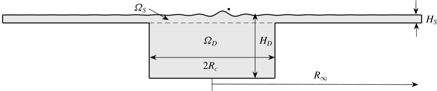
Schematic cross-sectional diagram of the circular corral configuration, where the fluid domain,  $\unicode[STIX]{x1D6FA}$, is the union of
 $\unicode[STIX]{x1D6FA}_{S}$ and
 $\unicode[STIX]{x1D6FA}_{D}$. The droplet is confined to the deep region. Effects of parasitic meniscus waves are contained within the shallow layer. The amplitude of the waves is exaggerated for visualisation of the free surface. Gilet (Reference Gilet2016) considered the cylindrical domain
 $R_{\infty }=R_{c}$, but we explore the case
 $R_{\infty }>R_{c}$ (Harris et al. Reference Harris, Moukhtar, Fort, Couder and Bush2013; Cristea-Platon, Sáenz & Bush Reference Cristea-Platon, Sáenz and Bush2018).

Submerged topography has been used in several prior experimental studies to provide controlled deviations from the droplet’s rectilinear walking state, mediated by topographically induced alterations to the guiding pilot wave. Examples include diffraction through slits (Couder & Fort Reference Couder and Fort2006; Andersen et al. Reference Andersen, Madsen, Reichelt, Rosenlund Ahl, Lautrup, Ellegaard, Levinsen and Bohr2015; Pucci et al. Reference Pucci, Harris, Faria and Bush2017), reflection and tunnelling over submerged walls (Eddi et al. Reference Eddi, Fort, Moisy and Couder2009; Pucci et al. Reference Pucci, Sáenz, Faria and Bush2016) and confinement to a cavity (Protière, Boudaoud & Couder Reference Protière, Boudaoud and Couder2006; Harris et al. Reference Harris, Moukhtar, Fort, Couder and Bush2013; Filoux, Hubert & Vandewalle Reference Filoux, Hubert and Vandewalle2015; Filoux et al. Reference Filoux, Hubert, Schlagheck and Vandewalle2017; Sáenz, Cristea-Platon & Bush Reference Sáenz, Cristea-Platon and Bush2018; Cristea-Platon et al. Reference Cristea-Platon, Sáenz and Bush2018). Of particular interest is the dynamics of a droplet confined by submerged topography to a circular cavity (henceforth, a ‘corral’), in which the droplet explores a deep, circular region, confined by the wave reflection off the surrounding submerged wall, as depicted in figure 1.
An array of dynamics may emerge for different values of the subcritical vibrational forcing. At short path memory, the wave reflection off the submerged wall acts as a non-local force on the droplet, resulting in the emergence of periodic orbits, typically characterised as circles, lemniscates and trefoils (Cristea-Platon et al. Reference Cristea-Platon, Sáenz and Bush2018). These trajectories exhibit a double quantisation in their mean radius and angular momentum, bearing similar dynamics to that of a droplet walking in a harmonic potential (Perrard et al. Reference Perrard, Labousse, Miskin, Fort and Couder2014b). Remarkably, the double quantisation of this hydrodynamic system has a form analogous to the double quantisation of the energy and angular momentum of a quantum particle. In this work, we rationalise the origins of dynamical similitude between these two contrasting configurations.
As the vibrational forcing is increased towards the Faraday threshold ( $\unicode[STIX]{x1D6E4}\rightarrow \unicode[STIX]{x1D6E4}_{F}^{-}$), the path memory necessarily increases and the droplet’s strong interaction with its wake, which fills the domain, results in a chaotic dynamics. In this latter regime, it has been shown that the long-time statistical distribution for the droplet’s position is multimodal in certain circumstances, with a statistical length scale prescribed by the Faraday wavelength,
 $\unicode[STIX]{x1D706}_{F}$ (Harris et al. Reference Harris, Moukhtar, Fort, Couder and Bush2013). This wave-like statistical form is analogous to that of quantum electrons moving in a quantum corral, where the Faraday wavelength plays the role of the de Broglie wavelength.
Unlike earlier studies of the pilot-wave dynamics in an unbounded domain, submerged topography considerably increases the computational expense of evolving the fluid equations. Even when using a linearised, weakly viscous, quasi-potential fluid model (Dias, Dyachenko & Zakharov Reference Dias, Dyachenko and Zakharov2008), one must solve Laplace’s equation for the velocity potential,  $\unicode[STIX]{x1D719}$, in the confining geometry in order to evolve the system. To reduce the problem to computations on the linearised free surface,
 $z=0$, one may construct the Dirichlet-to-Neumann (DtN) map, allowing the Neumann data,
 $\unicode[STIX]{x1D719}_{z}|_{z=0}$, to be determined by the Dirichlet data,
 $\unicode[STIX]{x1D719}|_{z=0}$, as is required for the kinematic boundary condition. However, computation of this map is difficult for complex, three-dimensional geometries, and, in contrast to the flat bottom or infinite-depth cases, the DtN map in the corral is not diagonal in the wavenumber,
 $k$, under a standard spectral decomposition.
To alleviate the difficulty of computing the DtN map for the corral geometry, Gilet (Reference Gilet2016) treated the submerged step as a no-flux (Neumann) boundary condition, maintaining the benefits of a diagonal system in the wavenumber,  $k$, for a cylindrical domain. However, this approximation fails to trap the droplet, which may sometimes escape the cavity. Indeed, the whole hydrodynamic evolution of the wave field is likely to be unsatisfactory under such a simple approximation, as the reflection, transmission and damping of the waves are not properly treated.
Computation of the DtN map for two-dimensional, polygonal geometries can be achieved using Schwarz–Christoffel conformal mapping, as was used by Nachbin, Milewski & Bush (Reference Nachbin, Milewski and Bush2017) and Nachbin (Reference Nachbin2018). For three-dimensional geometry, Faria (Reference Faria2017) proposed an ad hoc approximation of the DtN map, in which the map is tuned to match the phase speed of the Faraday waves in regions of constant depth. While this approximation has allowed for favourable agreement with pilot-wave experiments in a number of geometries (Pucci et al. Reference Pucci, Sáenz, Faria and Bush2016, Reference Pucci, Harris, Faria and Bush2017; Harris et al. Reference Harris, Brun, Damiano, Faria and Bush2018), the computations rely on viscosity to damp spurious high frequencies excited at sharp changes in depth.
In contrast, we seek a more general formulation that can be applied to a wide range of inviscid and weakly viscous wave problems, and develop a theoretical model for describing the Faraday pilot-wave dynamics under confinement to a circular corral. While some inferences have been made of the pilot-wave dynamics in specific topographical configurations (Pucci et al. Reference Pucci, Sáenz, Faria and Bush2016; Harris et al. Reference Harris, Brun, Damiano, Faria and Bush2018), we devise a framework amenable to analysis and efficient numerical simulations, shedding light on a class of problems in which few precise statements have been made. Specifically, we aim to characterise the form of the Faraday waves in a circular corral, rationalise the origins for the beguiling similarity between the observed pilot-wave dynamics in a harmonic potential (Perrard et al. Reference Perrard, Labousse, Fort and Couder2014a,Reference Perrard, Labousse, Miskin, Fort and Couderb) and a circular corral (Cristea-Platon et al. Reference Cristea-Platon, Sáenz and Bush2018) and probe regimes previously unexplored in experiments. Furthermore, our broad exploration of this pilot-wave system allows us to buttress prior experimental observations, specify regimes of future study and pin-point suitable refinements to the fluid mechanical model.
The paper is arranged as follows: in § 2, we present a formulation of the DtN map for the corral geometry. Upon assuming instantaneous, periodic point impacts, we derive a discrete-time iterative map to describe the evolution of the pilot-wave system in the corral, whose properties are analysed in § 3. We proceed by studying the linear stability of stationary bouncing and circular orbits in § 4, and rationalise the onset of orbital quantisation in the long-path-memory limit. Finally, we present a thorough simulation study of the pilot-wave dynamics in § 5, in which we see the emergence of exotic periodic orbits and the onset of chaos.
2 Model derivation
To model the fluid evolution over submerged topography, we make two simplifications to formulate a tractable system. First, we employ the linearised quasi-potential flow approximation within the fluid bulk, which involves neglecting the higher-order dissipation term in the dynamic boundary condition (Dias et al. Reference Dias, Dyachenko and Zakharov2008; Milewski et al. Reference Milewski, Galeano-Rios, Nachbin and Bush2015; Galeano-Rios, Milewski & Vanden-Broeck Reference Galeano-Rios, Milewski and Vanden-Broeck2017). Under this approximation, the vortical component of velocity decouples from the evolution of the velocity potential and the free-surface elevation, representing a significant computational saving. We note, however, that this quasi-potential model does not assume that the fluid motion is irrotational.
The second approximation is to neglect the no-slip condition on the submerged topography, akin to previous works (Faria Reference Faria2017; Nachbin et al. Reference Nachbin, Milewski and Bush2017; Nachbin Reference Nachbin2018). This approximation is reasonable when the topography is sufficiently deep relative to the length scale over which the submerged topography influences the dynamics of the fluid bulk. Specifically, for kinematic viscosity  $\unicode[STIX]{x1D708}$, fluid depth
 $H$ and vibrational forcing with angular frequency
 $\unicode[STIX]{x1D714}_{0}=2\unicode[STIX]{x03C0}f_{0}$, the departure from potential-like flow for subharmonic Faraday waves is described by the dimensionless parameter
 $\unicode[STIX]{x1D6FF}=\sqrt{\unicode[STIX]{x1D708}/\unicode[STIX]{x1D714}_{0}H^{2}}$ (Cerda & Tirapegui Reference Cerda and Tirapegui1998). For weak penetration of the fluid evolution due to the effect of the boundaries, we require
 $\unicode[STIX]{x1D6FF}\ll 1$. With the experimental parameters used by Harris et al. (Reference Harris, Moukhtar, Fort, Couder and Bush2013), namely
 $\unicode[STIX]{x1D708}=2\times 10^{-5}~\text{m}^{2}~\text{s}^{-1}$, vibrational frequency
 $f_{0}=80~\text{Hz}$, shallow depth
 $H_{S}=0.6~\text{mm}$ and deep depth
 $H_{D}=6.6~\text{mm}$, we find that
 $\unicode[STIX]{x1D6FF}$ in these two regions takes the values
 $\unicode[STIX]{x1D6FF}_{S}\approx 0.33$ and
 $\unicode[STIX]{x1D6FF}_{D}\approx 0.03$, respectively. While
 $\unicode[STIX]{x1D6FF}_{S}$ is hardly negligible in this regime, we demonstrate that our model captures the main features of the pilot-wave system, chiefly because the submerged walls confine the droplet to the deep region of the bath, where viscous effects due to the boundaries can be safely neglected.
As shown in figure 1, for  $\boldsymbol{x}=(x,y)^{\text{T}}$, we consider a finite domain
 $(\boldsymbol{x},z)\in \unicode[STIX]{x1D6FA}_{S}\cup \unicode[STIX]{x1D6FA}_{D}$, where the shallow layer is
 $\unicode[STIX]{x1D6FA}_{S}=\{(\boldsymbol{x},z)\,:\,|\boldsymbol{x}|<R_{\infty },z\in (-H_{S},0)\}$ and the deep region is
 $\unicode[STIX]{x1D6FA}_{D}=\{(\boldsymbol{x},z)\,:\,|\boldsymbol{x}|<R_{c},z\in (-H_{D},-H_{S})\}$. The outer radius,
 $R_{\infty }$, is large enough to guarantee that the fluid is undisturbed at the outer boundary.
We describe the fluid evolution in dimensionless variables. The corral radius,  $R_{c}$, is the most natural length scale; the Faraday wavelength is not clearly defined (due to coupling of wavenumbers) and we explore the effect of changing the forcing frequency,
 $f_{0}$. Thus, we scale
 $(\boldsymbol{x},z)\sim R_{c}$ and time with the Faraday period,
 $t\sim T_{F}=4\unicode[STIX]{x03C0}/\unicode[STIX]{x1D714}_{0}=2/f_{0}$. For a droplet of mass
 $m_{0}$, the natural pressure scale is
 $P_{0}\sim m_{0}g/R_{c}^{2}$, which supplies a balance with the free-surface elevation,
 $\unicode[STIX]{x1D702}(\boldsymbol{x},t)$, and velocity potential,
 $\unicode[STIX]{x1D719}(\boldsymbol{x},z,t)$, namely
 $\unicode[STIX]{x1D702}\sim Z_{0}$ and
 $\unicode[STIX]{x1D719}\sim Z_{0}R_{c}/T_{F}$, where
 $Z_{0}=m_{0}gT_{F}^{2}/(\unicode[STIX]{x1D70C}R_{c}^{3})$,
 $\unicode[STIX]{x1D70C}$ is the fluid density and
 $g$ is the gravitational acceleration. The dimensionless height of each layer is
 $h_{s}=H_{S}/R_{c}$ and
 $h_{d}=H_{D}/R_{c}$, and the dimensionless far-field radius is
 $r_{\infty }=R_{\infty }/R_{c}$.
The dimensionless equations for linearised quasi-potential flow (Dias et al. Reference Dias, Dyachenko and Zakharov2008) in the corral domain,  $\unicode[STIX]{x1D6FA}=\unicode[STIX]{x1D6FA}_{S}\cup \unicode[STIX]{x1D6FA}_{D}$, written in the vibrating frame of reference, are
 $$\begin{eqnarray}\displaystyle & 0=\unicode[STIX]{x0394}\unicode[STIX]{x1D719}+\unicode[STIX]{x1D719}_{zz},\quad (\boldsymbol{x},z)\in \unicode[STIX]{x1D6FA}, & \displaystyle\end{eqnarray}$$
 $$\begin{eqnarray}\displaystyle & \unicode[STIX]{x1D719}_{t}=-G(1-\unicode[STIX]{x1D6E4}\cos (4\unicode[STIX]{x03C0}t))\unicode[STIX]{x1D702}+Bo\,\unicode[STIX]{x0394}\unicode[STIX]{x1D702}+2Re^{-1}\unicode[STIX]{x0394}\unicode[STIX]{x1D719}-P_{0},\quad z=0,|\boldsymbol{x}|<r_{\infty }, & \displaystyle\end{eqnarray}$$
 $$\begin{eqnarray}\displaystyle & \unicode[STIX]{x1D702}_{t}=\unicode[STIX]{x1D719}_{z}+2Re^{-1}\unicode[STIX]{x0394}\unicode[STIX]{x1D702},\quad z=0,|\boldsymbol{x}|<r_{\infty }, & \displaystyle\end{eqnarray}$$
 $\unicode[STIX]{x1D6E5}=\unicode[STIX]{x2202}_{xx}+\unicode[STIX]{x2202}_{yy}$ is the horizontal Laplacian operator. The system’s dimensionless parameters are the Reynolds number
 $Re=R_{c}^{2}/\unicode[STIX]{x1D708}T_{F}$, Bond number
 $Bo\,=\unicode[STIX]{x1D70E}T_{F}^{2}/\unicode[STIX]{x1D70C}R_{c}^{3}$, inverse-squared Froude number
 $G=gT_{F}^{2}/R_{c}$ and the reduced acceleration
 $\unicode[STIX]{x1D6E4}=A\unicode[STIX]{x1D714}_{0}^{2}/g$, with forcing amplitude
 $A$, fluid kinematic viscosity
 $\unicode[STIX]{x1D708}$ and surface tension
 $\unicode[STIX]{x1D70E}$. One may model an applied pressure,
 $P_{0}(\boldsymbol{x},t)$, arising during droplet impact, but we instead prescribe
 $P_{0}$ through the wave–droplet coupling discussed below.
The free surface,  $\unicode[STIX]{x1D702}$, and the velocity potential,
 $\unicode[STIX]{x1D719}$, also obey the boundary conditions
 $$\begin{eqnarray}\displaystyle & \unicode[STIX]{x1D702}=0\quad \text{at }|\boldsymbol{x}|=r_{\infty }, & \displaystyle\end{eqnarray}$$
 $$\begin{eqnarray}\displaystyle & \unicode[STIX]{x1D719}=0\quad \text{on }|\boldsymbol{x}|=r_{\infty },z\in (-h_{s},0), & \displaystyle\end{eqnarray}$$
 $$\begin{eqnarray}\displaystyle & \unicode[STIX]{x2202}_{n}\unicode[STIX]{x1D719}=0\quad \text{on }|\boldsymbol{x}|=1,z\in (-h_{d},-h_{s}), & \displaystyle\end{eqnarray}$$
 $$\begin{eqnarray}\displaystyle & \unicode[STIX]{x2202}_{n}\unicode[STIX]{x1D719}=0\quad \text{on }z=-h_{d},|\boldsymbol{x}|\in [0,1), & \displaystyle\end{eqnarray}$$
 $$\begin{eqnarray}\displaystyle & \unicode[STIX]{x2202}_{n}\unicode[STIX]{x1D719}=0\quad \text{on }z=-h_{s},|\boldsymbol{x}|\in [1,r_{\infty }), & \displaystyle\end{eqnarray}$$
 $|\boldsymbol{x}|\rightarrow 0$, and
 $\unicode[STIX]{x2202}_{n}$ denotes the directional derivative operator along a unit vector normal to the corresponding surface.
To describe the droplet’s horizontal motion, we employ the model of Moláček & Bush (Reference Moláček and Bush2013). In dimensionless variables, the droplet’s position,  $\boldsymbol{X}(t)$, is governed by
 $$\begin{eqnarray}\boldsymbol{X}^{\prime \prime }(t)+(C_{a}+C_{i}\,f(t))\boldsymbol{X}^{\prime }(t)=-\unicode[STIX]{x1D6FF}_{0}Gf(t)\unicode[STIX]{x1D735}\unicode[STIX]{x1D702}(\boldsymbol{X}(t),t),\end{eqnarray}$$
where  $f(t)$ is a prescribed reaction force, which is zero during flight and positive during impact. The dimensionless coefficients
 $C_{i}=cgT_{F}\sqrt{\unicode[STIX]{x1D70C}R_{0}/\unicode[STIX]{x1D70E}}$ and
 $C_{a}=6\unicode[STIX]{x03C0}R_{0}\unicode[STIX]{x1D707}_{a}T_{F}/m_{0}$ describe the drag due to skidding friction and air drag, while
 $\unicode[STIX]{x1D6FF}_{0}=Z_{0}/R_{c}$ is a length-scale ratio. Here,
 $R_{0}$ and
 $m_{0}=\frac{4}{3}\unicode[STIX]{x03C0}\unicode[STIX]{x1D70C}R_{0}^{3}$ are the dimensional radius and mass of the droplet, respectively,
 $\unicode[STIX]{x1D707}_{a}=1.8\times 10^{-5}~\text{kg}~\text{m}^{-1}~\text{s}^{-1}$ is the dynamic viscosity of air and
 $c=0.17$ is an empirically deduced skidding friction coefficient (Moláček & Bush Reference Moláček and Bush2013).
To derive a tractable model, which we recast as a discrete-time iterative map in § 2.3, we proceed to make several simplifications. Consistent with experimental observations of walkers (Couder et al. Reference Couder, Protière, Fort and Boudaoud2005b; Protière et al. Reference Protière, Couder, Fort and Boudaoud2005, Reference Protière, Boudaoud and Couder2006; Eddi et al. Reference Eddi, Sultan, Moukhtar, Fort, Rossi and Couder2011; Moláček & Bush Reference Moláček and Bush2013; Wind-Willassen et al. Reference Wind-Willassen, Moláček, Harris and Bush2013), we prescribe the droplet’s vertical motion as periodic and subharmonic relative to the vibrational forcing. Moreover, as the impact duration of walkers is typically short relative to the bouncing period (Protière et al. Reference Protière, Boudaoud and Couder2006), we reduce the wave–droplet coupling to an instant in time, which has been shown to be a practical simplification in prior works (Durey & Milewski Reference Durey and Milewski2017; Faria Reference Faria2017). Lastly, as the droplet radius is small compared to a typical wavelength, and short waves are rapidly damped, we model the pressure,  $P_{0}$, as a point in space.
The assumption of subharmonic, periodic impacts implies that the time-averaged normal force balances with the droplet’s weight (Moláček & Bush Reference Moláček and Bush2013). Hence, we prescribe the dimensionless pressure distribution as  $P_{0}(\boldsymbol{x},t)=f(t)\unicode[STIX]{x1D6FF}(\boldsymbol{x}-\boldsymbol{X}(t))$, where
 $f(t)=\sum _{n=0}^{\infty }\unicode[STIX]{x1D6FF}(t-t_{n})$ is the dimensionless normal force,
 $t_{n}=n+\unicode[STIX]{x1D703}_{I}/(4\unicode[STIX]{x03C0})$ for all
 $n\geqslant 0$ and the droplet impact phase,
 $\unicode[STIX]{x1D703}_{I}$, is a free parameter of the model. The instantaneous forcing gives rise to jump conditions in
 $\unicode[STIX]{x1D719}$ and
 $\boldsymbol{X}^{\prime }$ at each impact, as discussed in § 2.3.
Throughout this work, we consider silicone oil with kinematic viscosity  $\unicode[STIX]{x1D708}=2\times 10^{-5}~\text{m}^{2}~\text{s}^{-1}$, density
 $\unicode[STIX]{x1D70C}=949~\text{kg}~\text{m}^{-3}$ and surface tension
 $\unicode[STIX]{x1D70E}=2.06\times 10^{-2}~\text{kg}~\text{s}^{-2}$. To match the predictions of the quasi-potential flow model with the experimentally observed Faraday threshold,
 $\unicode[STIX]{x1D6E4}_{F}=4.22$, in an unbounded domain with
 $f_{0}=80~\text{Hz}$ (Wind-Willassen et al. Reference Wind-Willassen, Moláček, Harris and Bush2013), Milewski et al. (Reference Milewski, Galeano-Rios, Nachbin and Bush2015) introduced the viscosity correction
 $\unicode[STIX]{x1D708}\mapsto 0.8025\unicode[STIX]{x1D708}$. As the temporal decay of the Faraday waves depends primarily on the ratio
 $\unicode[STIX]{x1D6E4}/\unicode[STIX]{x1D6E4}_{F}$, this fluid model has been used to successfully reproduce a number of experimentally observed phenomena (see, for example, Pucci et al. (Reference Pucci, Sáenz, Faria and Bush2016, Reference Pucci, Harris, Faria and Bush2017), Faria (Reference Faria2017), Galeano-Rios et al. (Reference Galeano-Rios, Milewski and Vanden-Broeck2017), Nachbin et al. (Reference Nachbin, Milewski and Bush2017), Galeano-Rios, Milewski & Vanden-Broeck (Reference Galeano-Rios, Milewski and Vanden-Broeck2019) and Harris et al. (Reference Harris, Brun, Damiano, Faria and Bush2018)). We also adopt this viscosity correction, although we do not account for any additional viscous effects that may arise due to interaction with the submerged topography.
Equations (2.1)–(2.2) are challenging to evolve in a numerically efficient manner as one must solve Laplace’s equation in the domain,  $\unicode[STIX]{x1D6FA}$, for the velocity potential,
 $\unicode[STIX]{x1D719}$. In § 2.1, we reduce the dynamics to the surface by constructing the DtN operator,
 ${\mathcal{N}}[\unicode[STIX]{x1D719}|_{z=0}]=\unicode[STIX]{x1D719}_{z}|_{z=0}$. (The reader only interested in the application of this operator may proceed to § 2.2.) To further increase the numerical efficiency, we then exploit the fact that the wave–droplet coupling is confined to an instant in time, allowing us to reformulate the dynamics as a discrete-time iterative map, as derived in § 2.3.
2.1 The Dirichlet-to-Neumann map
To numerically compute the DtN map in the corral geometry, we employ a domain decomposition method. In simple geometries, there are known analytical solutions to Laplace’s equation. In certain complex geometries that are composed of combinations of such simple geometries, the domain decomposition method is particularly effective since the known solutions form the building blocks of the DtN map. In our case, the corral is the union of two cylinders. By using a Hankel transform to solve Laplace’s equation analytically in each cylindrical sub-domain, and using appropriate matching, one obtains the required DtN map for the full domain. This method also applies to the annular cavity (Filoux et al. Reference Filoux, Hubert and Vandewalle2015) and submerged pillar (Harris et al. Reference Harris, Brun, Damiano, Faria and Bush2018) configurations.
Other problems can also be approached this way: when each sub-domain instead has a rectangular cross-section, such as for planar steps (Pucci et al. Reference Pucci, Sáenz, Faria and Bush2016), square corrals (Protière et al. Reference Protière, Boudaoud and Couder2006; Eddi et al. Reference Eddi, Fort, Moisy and Couder2009) or linear channels (Harris Reference Harris2015; Filoux et al. Reference Filoux, Hubert, Schlagheck and Vandewalle2017), a domain decomposition based on Fourier modes is appropriate. Furthermore, elliptical corrals (Sáenz et al. Reference Sáenz, Cristea-Platon and Bush2018) can be studied using elliptical coordinates (corresponding to Mathieu functions). The efficiency of the method can be further increased when each sub-geometry exhibits either rotational or translational invariance, as discussed below.
We first decompose the velocity potential,  $\unicode[STIX]{x1D719}$, for each sub-domain
 $$\begin{eqnarray}\unicode[STIX]{x1D719}=\left\{\begin{array}{@{}l@{}}\unicode[STIX]{x1D719}^{S},\quad (\boldsymbol{x},z)\in \unicode[STIX]{x1D6FA}_{S},\quad \\ \unicode[STIX]{x1D719}^{D},\quad (\boldsymbol{x},z)\in \unicode[STIX]{x1D6FA}_{D}.\quad \end{array}\right.\end{eqnarray}$$
Both  $\unicode[STIX]{x1D719}^{S}$ and
 $\unicode[STIX]{x1D719}^{D}$ satisfy Laplace’s equation in their respective domains, equipped with boundary conditions consistent with (2.2). At each instant in time, the aim is to solve for
 $\unicode[STIX]{x1D719}$ given Dirichlet data
 $\unicode[STIX]{x1D719}|_{z=0}=a(\boldsymbol{x})$, from which we determine the corresponding Neumann data,
 $\unicode[STIX]{x1D719}_{z}|_{z=0}$. To solve for
 $\unicode[STIX]{x1D719}^{S}$ and
 $\unicode[STIX]{x1D719}^{D}$ concurrently, we introduce the unknown functions
 $b^{S}(\boldsymbol{x})$ and
 $b^{D}(\boldsymbol{x})$, satisfying
 $$\begin{eqnarray}\unicode[STIX]{x1D719}^{S}=b^{S}\quad \text{and}\quad \unicode[STIX]{x1D719}^{D}=b^{D}\quad \text{on }z=-h_{s}.\end{eqnarray}$$
The functions  $b^{S}(\boldsymbol{x})$ and
 $b^{D}(\boldsymbol{x})$ are chosen to be consistent with the fluid flow, specifically
 $$\begin{eqnarray}\displaystyle & b^{S}=b^{D}\quad \text{for }|\boldsymbol{x}|<1, & \displaystyle \nonumber\\ \displaystyle & \unicode[STIX]{x2202}_{z}\unicode[STIX]{x1D719}^{S}=\unicode[STIX]{x2202}_{z}\unicode[STIX]{x1D719}^{D}\quad \text{on }z=-h_{s},|\boldsymbol{x}|<1, & \displaystyle \nonumber\\ \displaystyle & \unicode[STIX]{x2202}_{z}\unicode[STIX]{x1D719}^{S}=0\quad \text{on }z=-h_{s},|\boldsymbol{x}|\in [1,r_{\infty }). & \displaystyle \nonumber\end{eqnarray}$$
Upon solving for  $b^{S}$, one can determine
 $\unicode[STIX]{x1D719}^{S}$ and hence
 $\unicode[STIX]{x1D719}_{z}^{S}|_{z=0}$, completing the DtN map.
The inversion for  $b^{S}$ and
 $b^{D}$ can be simplified when the domain exhibits rotational or translational invariance, as is the case for circular corrals, infinitely long rectilinear channels and annular cavities. Upon appropriate discretisation, this invariance allows one to divide the domain decomposition method into a series of problems of much smaller size (for which computations may be parallelised), significantly reducing the computational cost. We proceed to describe this method for a circular corral, the domain of interest in this study. (The implementations of the DtN map for an annular channel and an infinite-length, rectilinear channel are presented in the supplementary material available at https://doi.org/10.1017/jfm.2020.140.)
To analytically solve for  $\unicode[STIX]{x1D719}^{S}$ and
 $\unicode[STIX]{x1D719}^{D}$ in the circular corral geometry, we introduce cylindrical polar coordinates
 $(r,\unicode[STIX]{x1D703},z)$. We proceed by expanding
 $\unicode[STIX]{x1D719}^{S}$,
 $\unicode[STIX]{x1D719}^{D}$,
 $a$,
 $b^{S}$ and
 $b^{D}$ into Fourier angular modes, for example
 $\unicode[STIX]{x1D719}^{S}(r,\unicode[STIX]{x1D703},z)=\sum _{m=-\infty }^{\infty }\unicode[STIX]{x1D719}_{m}^{S}(r,z)\text{e}^{\text{i}m\unicode[STIX]{x1D703}}$, where
 $\text{i}^{2}=-1$. As
 $\unicode[STIX]{x1D719}^{S}$ and
 $\unicode[STIX]{x1D719}^{D}$ are both harmonic functions, it is necessary to solve
 $$\begin{eqnarray}\displaystyle & {\mathcal{L}}_{m}\unicode[STIX]{x1D719}_{m}^{S}=0,\quad \text{for }(r,z)\in [0,r_{\infty })\times (-h_{s},0), & \displaystyle \nonumber\\ \displaystyle & {\mathcal{L}}_{m}\unicode[STIX]{x1D719}_{m}^{D}=0,\quad \text{for }(r,z)\in [0,1)\times (-h_{d},-h_{s}), & \displaystyle \nonumber\end{eqnarray}$$
where  ${\mathcal{L}}_{m}=\unicode[STIX]{x2202}_{rr}+r^{-1}\unicode[STIX]{x2202}_{r}+\unicode[STIX]{x2202}_{zz}-(m/r)^{2}$ is Laplace’s operator for angular mode
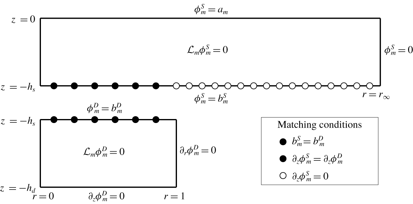
 $m$. As depicted in figure 2, the boundary conditions for the shallow region are
 $\unicode[STIX]{x1D719}_{m}^{S}=0$ on
 $r=r_{\infty }$,
 $\unicode[STIX]{x1D719}_{m}^{S}=a_{m}$ on
 $z=0$,
 $\unicode[STIX]{x1D719}_{m}^{S}=b_{m}^{S}$ on
 $z=-h_{s}$, with
 $\unicode[STIX]{x1D719}_{m}^{S}$ bounded as
 $r\rightarrow 0$. Similarly, we require
 $\unicode[STIX]{x2202}_{r}\unicode[STIX]{x1D719}_{m}^{D}=0$ on
 $r=1$,
 $\unicode[STIX]{x1D719}_{m}^{D}=b_{m}^{D}$ on
 $z=-h_{s}$,
 $\unicode[STIX]{x2202}_{z}\unicode[STIX]{x1D719}_{m}^{D}=0$ on
 $z=-h_{d}$ and boundedness of
 $\unicode[STIX]{x1D719}_{m}^{D}$ as
 $r\rightarrow 0$.
Cross-sectional schematic diagram of the domain decomposition method used to compute the DtN map. The circles indicate the  $N_{S}$ radial collocation points,
 $\unicode[STIX]{x1D70C}_{j}$, with black circles for
 $j\leqslant N_{D}$ and white circles for
 $j>N_{D}$. The differential operator is
 ${\mathcal{L}}_{m}=\unicode[STIX]{x2202}_{rr}+r^{-1}\unicode[STIX]{x2202}_{r}+\unicode[STIX]{x2202}_{zz}-(m/r)^{2}$. At
 $r=0$, we seek a bounded solution.

We first solve for  $\unicode[STIX]{x1D719}_{m}^{S}$ and
 $\unicode[STIX]{x1D719}_{m}^{D}$ before determining
 $b_{m}^{S}$ and
 $b_{m}^{D}$ according to the matching conditions. To solve
 ${\mathcal{L}}_{m}\unicode[STIX]{x1D719}_{m}^{S}=0$ with respect to the radial boundary conditions, we employ the Hankel transform
 $\unicode[STIX]{x1D719}_{m}^{S}(r,z)=\sum _{p=1}^{\infty }\unicode[STIX]{x1D719}_{mp}^{S}(z)\text{J}_{m}(k_{mp}^{S}r)$ (similarly for
 $b_{m}^{S}$ and
 $a_{m}$), where
 $\text{J}_{m}(x)$ is the Bessel function of the first kind of order
 $m$. The distinct wavenumbers
 $k_{mp}^{S}>0$ satisfy the Dirichlet boundary condition (2.2b) at
 $r=r_{\infty }$, specifically
 $\text{J}_{m}(k_{mp}^{S}r_{\infty })=0$. The analytic solution for
 $\unicode[STIX]{x1D719}_{m}^{S}(r,z)$ is then
 $$\begin{eqnarray}\unicode[STIX]{x1D719}_{m}^{S}(r,z)=\mathop{\sum }_{p=1}^{\infty }\left[a_{mp}\frac{\sinh (k_{mp}^{S}(z+h_{s}))}{\sinh (k_{mp}^{S}h_{s})}-b_{mp}^{S}\frac{\sinh (k_{mp}^{S}z)}{\sinh (k_{mp}^{S}h_{s})}\right]\text{J}_{m}(k_{mp}^{S}r).\end{eqnarray}$$
In the deep region, the radial boundary conditions determine the Hankel transform  $\unicode[STIX]{x1D719}_{m}^{D}(r,z)=\sum _{p=1}^{\infty }\unicode[STIX]{x1D719}_{mp}^{D}(z)\text{J}_{m}(k_{mp}^{D}r)$, where the distinct wavenumbers
 $k_{mp}^{D}\geqslant 0$ satisfy
 $\text{J}_{m}^{\prime }(k_{mp}^{D})=0$. This problem yields the well-known DtN map for finite depth, namely
 $\unicode[STIX]{x2202}_{z}\unicode[STIX]{x1D719}_{mp}^{D}(-h_{s})=b_{mp}^{D}k_{mp}^{D}\tanh (k_{mp}^{D}(h_{d}-h_{s}))$. Hence,
 $$\begin{eqnarray}\unicode[STIX]{x2202}_{z}\unicode[STIX]{x1D719}_{m}^{D}(r,-h_{s})=\mathop{\sum }_{p=1}^{\infty }b_{mp}^{D}k_{mp}^{D}\tanh (k_{mp}^{D}(h_{d}-h_{s}))\text{J}_{m}(k_{mp}^{D}r).\end{eqnarray}$$
To match the velocity potential along  $z=-h_{s}$ for each angular mode
 $m$, we utilise
 $N_{S}$ radial collocation points
 $\unicode[STIX]{x1D70C}_{j}$, where
 $0\leqslant \unicode[STIX]{x1D70C}_{1}<\unicode[STIX]{x1D70C}_{2}<\cdots <\unicode[STIX]{x1D70C}_{N_{S}}<r_{\infty }$, which we define in appendix A. To satisfy the velocity continuity between the domains
 $\unicode[STIX]{x1D6FA}_{S}$ and
 $\unicode[STIX]{x1D6FA}_{D}$, as well as the no-flux condition through the base of the corral (see (2.2e)), at each radial collocation point,
 $\unicode[STIX]{x1D70C}_{j}$, we require
 $$\begin{eqnarray}\displaystyle & b_{m}^{S}=b_{m}^{D},\quad \unicode[STIX]{x1D70C}_{j}\in [0,1), & \displaystyle\end{eqnarray}$$
 $$\begin{eqnarray}\displaystyle & \unicode[STIX]{x2202}_{z}\unicode[STIX]{x1D719}_{m}^{S}=\unicode[STIX]{x2202}_{z}\unicode[STIX]{x1D719}_{m}^{D},\quad \unicode[STIX]{x1D70C}_{j}\in [0,1),z=-h_{s}, & \displaystyle\end{eqnarray}$$
 $$\begin{eqnarray}\displaystyle & \unicode[STIX]{x2202}_{z}\unicode[STIX]{x1D719}_{m}^{S}=0,\quad \unicode[STIX]{x1D70C}_{j}\in [1,r_{\infty }),z=-h_{s}. & \displaystyle\end{eqnarray}$$
 $N_{D}<N_{S}$ collocation points satisfy
 $\unicode[STIX]{x1D70C}_{j}<1$. For a well-posed problem, we must similarly truncate the wavenumbers
 $k_{mp}^{S}$ and
 $k_{mp}^{D}$ to
 $p\leqslant N_{S}$ and
 $p\leqslant N_{D}$ in the shallow and deep regions, respectively.
To satisfy conditions (2.6b)–(2.6c), we evaluate (2.4)–(2.5) at the collocation points, yielding a system of  $N_{S}$ equations for
 $b_{m1}^{S},\ldots ,b_{mN_{S}}^{S}$ and
 $b_{m1}^{D},\ldots ,b_{mN_{D}}^{D}$
 $$\begin{eqnarray}\displaystyle & & \displaystyle \mathop{\sum }_{p=1}^{N_{S}}(a_{mp}-b_{mp}^{S}\cosh (k_{mp}^{S}h_{s}))\frac{k_{mp}^{S}\text{J}_{m}(k_{mp}^{S}\unicode[STIX]{x1D70C}_{j})}{\sinh (k_{mp}^{S}h_{s})}\nonumber\\ \displaystyle & & \displaystyle \quad =\left\{\begin{array}{@{}ll@{}}\displaystyle \mathop{\sum }_{p=1}^{N_{D}}b_{mp}^{D}k_{mp}^{D}\tanh (k_{mp}^{D}(h_{d}-h_{s}))\text{J}_{m}(k_{mp}^{D}\unicode[STIX]{x1D70C}_{j}),\quad & j\leqslant N_{D},\\ 0,\quad & j>N_{D}.\end{array}\right.\end{eqnarray}$$
To close the system, the continuity condition (2.6a) gives
 $$\begin{eqnarray}\mathop{\sum }_{p=1}^{N_{S}}b_{mp}^{S}\text{J}_{m}(k_{mp}^{S}\unicode[STIX]{x1D70C}_{j})=\mathop{\sum }_{p=1}^{N_{D}}b_{mp}^{D}\text{J}_{m}(k_{mp}^{D}\unicode[STIX]{x1D70C}_{j}),\quad \forall j\leqslant N_{D}.\end{eqnarray}$$
For each  $m\in \mathbb{Z}$, equations (2.7)–(2.8) may be recast in the form
 $$\begin{eqnarray}\left(\begin{array}{@{}cc@{}}\unicode[STIX]{x1D63D} & \unicode[STIX]{x1D63E}\\ \unicode[STIX]{x1D63F} & \unicode[STIX]{x1D640}\end{array}\right)\left(\begin{array}{@{}c@{}}\boldsymbol{b}_{S}\\ \boldsymbol{b}_{D}\end{array}\right)=\left(\begin{array}{@{}c@{}}\unicode[STIX]{x1D63C}\boldsymbol{a}\\ \boldsymbol{ 0}\end{array}\right),\end{eqnarray}$$
where it remains to find vectors  $\boldsymbol{b}_{S}$ and
 $\boldsymbol{b}_{D}$ for given
 $\boldsymbol{a}$. Following the numerical computation of
 $b_{mp}^{S}$ and
 $b_{mp}^{D}$, equation (2.4) determines the DtN map
 $$\begin{eqnarray}\unicode[STIX]{x2202}_{z}\unicode[STIX]{x1D719}_{mp}^{S}(0)=k_{mp}^{S}(a_{mp}\coth (k_{mp}^{S}h_{s})-b_{mp}^{S}\,\text{cosech}(k_{mp}^{S}h_{s})).\end{eqnarray}$$
When repeatedly computing the DtN, we pre-compute the LU-decomposition (with partial pivoting) of the map’s mass matrix (see (2.9)).
The justification for truncating large wavenumbers relies on the shallow penetration depth of short waves, in which surface perturbations do not propagate to the sufficiently deep submerged topography. Although energy may be transferred from long to short waves across the step, the short waves continue to evolve as if the domain were of infinite depth and so do not significantly influence the wave evolution near the submerged step.
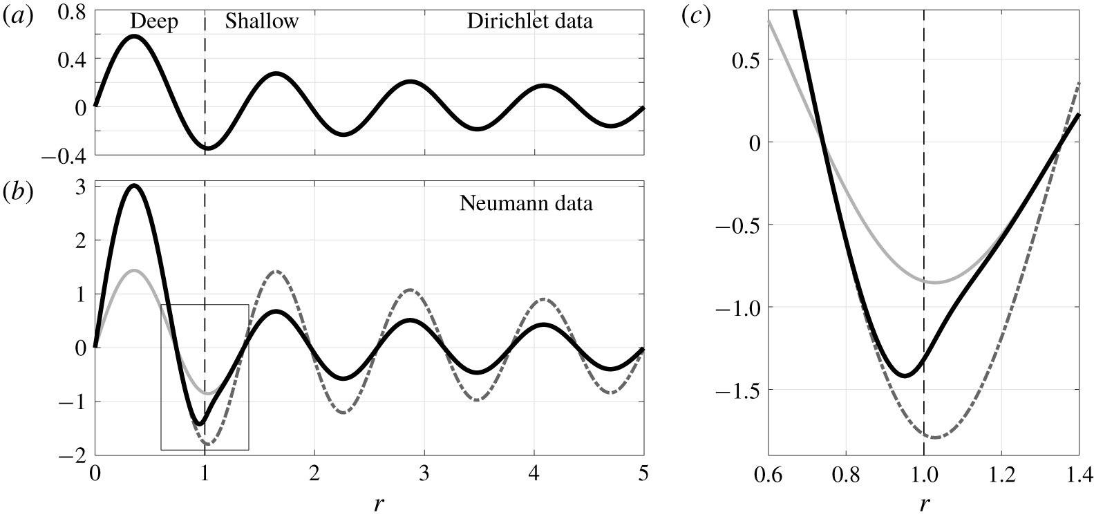
The DtN map for  $m=1$ with a step at
 $r=1$ (black dashed line), outer radius
 $r_{\infty }=5$ and depths
 $h_{d}=1$ and
 $h_{s}=0.1$. The submerged topography is not shown in the figure. (a) Example Dirichlet data
 $\unicode[STIX]{x1D719}_{1}^{S}(r,0)=\text{J}_{m}(k_{1,8}^{S}r)$. (b) The Neumann data,
 $\unicode[STIX]{x2202}_{z}\unicode[STIX]{x1D719}_{1}^{S}(r,0)$, for the corral geometry (black curve) computed using
 $N_{S}=512$ collocation points,
 $\unicode[STIX]{x1D70C}_{j}$. The corresponding data
 $\unicode[STIX]{x2202}_{z}\unicode[STIX]{x1D719}_{1}^{S}(r,0)$ for a cylindrical domain of radius
 $r_{\infty }$ with constant depth
 $h_{s}$ (light grey curve) and constant depth
 $h_{d}$ (dash-dotted curve). (c) Zoom-in of the rectangular box in panel
 $(b)$, showing that, for the corral,
 $\unicode[STIX]{x2202}_{z}\unicode[STIX]{x1D719}_{1}^{S}(r,0)$ coincides with the constant-depth cases away from the submerged step, with a smooth transition between the two solutions across
 $r=1$.

We present an example of the DtN map for the corral geometry in figure 3 for  $m=1$ and given Dirichlet data. Sufficiently far away from the submerged step, the Neumann data for the corral coincides with Neumann data for a cylindrical domain of constant depth
 $h$, with
 $h=h_{d}$ for
 $r<1$, and
 $h=h_{s}$ for
 $r>1$. In the vicinity of the step, the corral solution smoothly transitions between the two constant-depth solutions, over a length scale determined by the spatial non-locality of the operator. The self-convergence of this method as
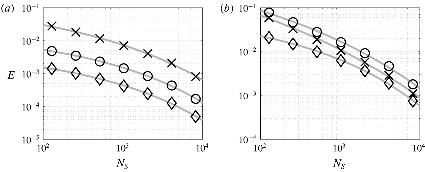
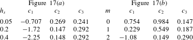
 $N_{S}\rightarrow \infty$ is discussed in § B.1, from which we deduce that
 $N_{S}=512$ is sufficient to accurately resolve the DtN map in the corral geometries considered.
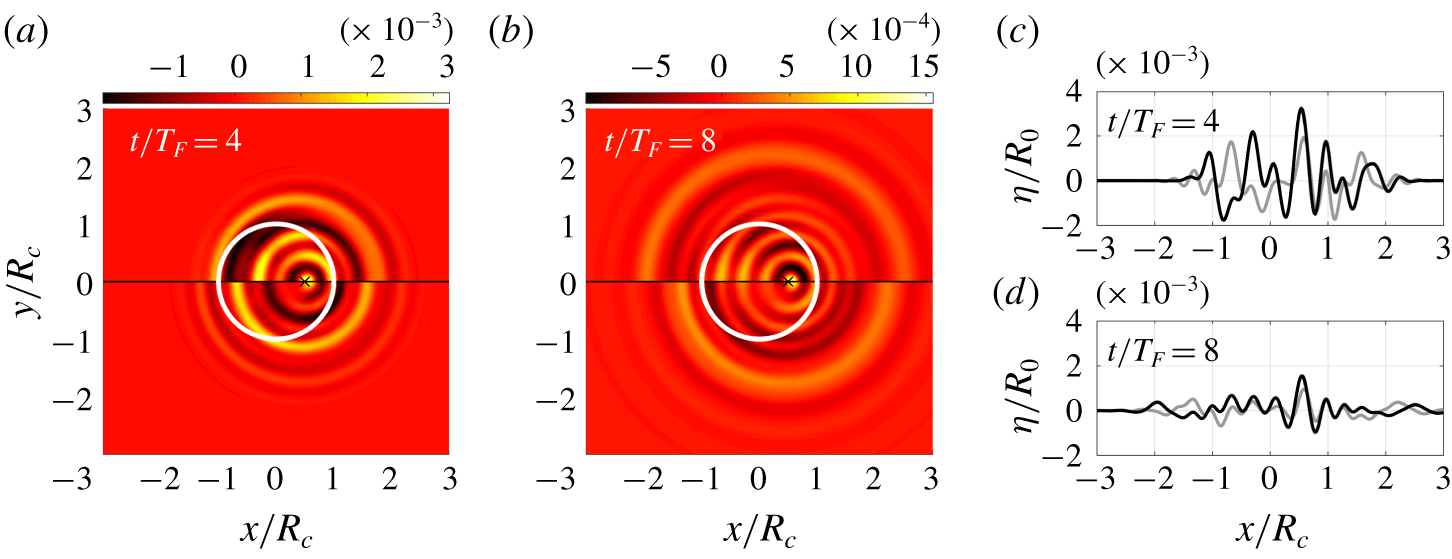
Comparison of the wave field generated by a single impact, evolved using our model and Faria’s model, for corral radius  $R_{c}=14~\text{mm}$, frequency
 $f_{0}=80~\text{Hz}$ and
 $\unicode[STIX]{x1D6E4}=4.1$ (corresponding to
 $\unicode[STIX]{x1D6E4}/\unicode[STIX]{x1D6E4}_{F}=0.9$ in our model). The free-surface elevation is normalised by the droplet radius,
 $R_{0}=0.35~\text{mm}$. The impact was at position
 $\boldsymbol{x}/R_{c}=(0.5,0)^{\text{T}}$, indicated by the cross in (a,b), with phase
 $\unicode[STIX]{x1D703}_{I}=1.43\unicode[STIX]{x03C0}$. (a,b) The computations of our model are presented for
 $y>0$, and Faria’s model for
 $y<0$, at times (a)
 $t/T_{F}=4$ and (b)
 $t/T_{F}=8$. The white circle denotes the submerged step. (c,d) The
 $y=0$ cross-section of our model (black) and Faria’s model (grey). The data in (c,d) are identical to (a,b).

Unlike the work of Faria (Reference Faria2017), our computation of the DtN map does not invoke jumps in the velocity potential across the step, making this approach applicable to inviscid flows, without relying on viscosity to dampen spurious short waves. Moreover, Faria’s method is specifically designed to approximate the evolution of Faraday waves, whereas our formulation may be applied to a broad class of water wave problems. We explore the effect of these approximations in § 2.2.
2.2 Comparison to a Faraday phase-speed-matched model
We compare the predictions of our model, with the computation of the DtN map described in § 2.1, to that of Faria (Reference Faria2017). In Faria’s model, the DtN map is replaced by the expression  $\unicode[STIX]{x1D719}_{z}|_{z=0}=-\unicode[STIX]{x1D735}\boldsymbol{\cdot }(b\unicode[STIX]{x1D735}\unicode[STIX]{x1D719}|_{z=0})$, where
 $b(\boldsymbol{x})$ is chosen to match the phase speed of the Faraday wavenumber in regions of constant depth. In dimensional variables,
 $b(\boldsymbol{x})$ takes the value
 $\tanh (k_{D}H_{D})/k_{D}$ in the deep region and
 $\tanh (k_{S}H_{S})/k_{S}$ in the shallow layer, where, for given
 $\unicode[STIX]{x1D6E4}$,
 $k_{D}$ and
 $k_{S}$ are the critical Faraday wavenumbers for flat-bottom domains of depth
 $H_{D}$ and
 $H_{S}$, respectively (Milewski et al. Reference Milewski, Galeano-Rios, Nachbin and Bush2015; Faria Reference Faria2017). Other than the DtN map, the two models are identical, but their implementation differs significantly.
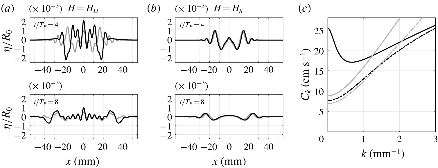
We consider the wave evolution arising from a single instantaneous point impact, which is the Green’s function for the corral geometry. The numerical implementation of our model is described in § 2.3, and Faria’s model is implemented using the Fourier pseudo-spectral method detailed in Faria (Reference Faria2017). As highlighted in figure 4, there are marked differences in the wave evolution, particularly at short times. To understand the origins of this discrepancy, we consider the same wave field generation but for a flat-bottom domain (with depth  $H_{D}$ or
 $H_{S}$) and infinite horizontal extent, the implementation of which is as described by Durey & Milewski (Reference Durey and Milewski2017). As presented in figure 5, similar discrepancies persist in the absence of submerged topography at depth
 $H_{D}$, but less so at depth
 $H_{S}$ (since Faria’s DtN map is inspired by shallow water theory), highlighting a fundamental difference in the wave evolution of these two models in the deep region. This difference is significant in the resulting pilot-wave dynamics, as the droplet is confined to the deep region of the corral, for which the wave field discrepancy is greatest.
Comparison of the axisymmetric wave field generated by a single impact over a flat-bottom domain with infinite horizontal extent, evolved using our model (black curves) and Faria’s model (grey curves) for  $f_{0}=80~\text{Hz}$,
 $\unicode[STIX]{x1D6E4}=3.8$ and
 $\unicode[STIX]{x1D703}_{I}=1.43\unicode[STIX]{x03C0}$. The free surface is normalised by the droplet radius,
 $R_{0}=0.35~\text{mm}$. (a) Depth
 $H_{D}=6.6~\text{mm}$. (b) Depth
 $H_{S}=0.6~\text{mm}$. (c) Phase speed of the unforced waves (
 $\unicode[STIX]{x1D6E4}=0$) for our model (
 $C_{k}$, black curves) and Faria’s model (
 $C_{k}^{F}$, grey curves). Solid and dash-dotted curves correspond to depths
 $H_{D}$ and
 $H_{S}$, respectively, with respective intersections at
 $k=k_{D}$ and
 $k=k_{S}$.

The differences at short time may be explained through consideration of the phase speed,  $C_{k}$, arising from the dispersion relation of (2.1) for wavenumber
 $k$ and
 $\unicode[STIX]{x1D6E4}=0$. Similarly,
 $C_{k}^{F}$ is the phase speed for Faria’s model. For constant depth
 $H$, we obtain
 $$\begin{eqnarray}C_{k}=\sqrt{\frac{\tanh (kH)}{k}\left(g+\frac{\unicode[STIX]{x1D70E}}{\unicode[STIX]{x1D70C}}k^{2}\right)}\quad \text{and}\quad C_{k}^{F}=\sqrt{\frac{\tanh (k_{F}H)}{k_{F}}\left(g+\frac{\unicode[STIX]{x1D70E}}{\unicode[STIX]{x1D70C}}k^{2}\right)},\end{eqnarray}$$
where  $k_{F}$ is the corresponding critical Faraday wavenumber (
 $k_{D}$ or
 $k_{S}$). As presented in figure 5(c),
 $C_{k}$ and
 $C_{k}^{F}$ agree only at
 $k=k_{F}$, where the difference is most apparent for deep fluid. Waves of intermediate length are only weakly damped at short times, playing a pivotal role in the wave field evolution. While the discrepancy between the two models may reduce when one considers subharmonic periodic impacts on the bath resonating with the Faraday frequency (Faria Reference Faria2017), short-time transient effects can strongly influence the pilot-wave dynamics of droplet–droplet interactions (Galeano-Rios, Couchman & Bush Reference Galeano-Rios, Couchman and Bush2018) or for dynamics very close to boundaries, where reflected transients are significant. Our method for computing the DtN map is thus particularly beneficial for modelling droplet–droplet dynamics confined by submerged topography, such as strings of propelling droplets (Filoux et al. Reference Filoux, Hubert and Vandewalle2015) and droplet lattices (Thomson, Couchman & Bush Reference Thomson, Couchman and Bush2020).
2.3 The discrete-time iterative map
We employ a similar decomposition to that of the previous section, expressing  $\boldsymbol{x}$ as
 $(r,\unicode[STIX]{x1D703})$ in plane-polar coordinates. Hence,
 $\unicode[STIX]{x1D702}$ and
 $\unicode[STIX]{x1D719}|_{z=0}$ are recast as
 $$\begin{eqnarray}\unicode[STIX]{x1D702}(\boldsymbol{x},t)=\mathop{\sum }_{m=-\infty }^{\infty }\mathop{\sum }_{p=1}^{\infty }\unicode[STIX]{x1D702}_{mp}(t)\unicode[STIX]{x1D6F7}_{mp}(\boldsymbol{x})\quad \text{and}\quad \unicode[STIX]{x1D719}(\boldsymbol{x},0,t)=\mathop{\sum }_{m=-\infty }^{\infty }\mathop{\sum }_{p=1}^{\infty }\unicode[STIX]{x1D719}_{mp}(t)\unicode[STIX]{x1D6F7}_{mp}(\boldsymbol{x}),\end{eqnarray}$$
with orthogonal basis functions  $\unicode[STIX]{x1D6F7}_{mp}(\boldsymbol{x})=\text{J}_{m}(k_{mp}^{S}r)\text{e}^{\text{i}m\unicode[STIX]{x1D703}}$. For tractable notation, we henceforth remove the superscript from
 $k_{mp}^{S}$. The reality condition for
 $\unicode[STIX]{x1D702}$ is
 $\unicode[STIX]{x1D702}_{-m,p}=(-1)^{m}\unicode[STIX]{x1D702}_{m,p}^{\ast }$, where
 $\ast$ denotes complex conjugation, and similarly for
 $\unicode[STIX]{x1D719}$.
By similarly expressing the pressure,  $P_{0}(\boldsymbol{x},t)$, in terms of the transformed variables
 $P_{mp}(t)$, the dimensionless governing fluid equations (2.1) reduce to the system
 $$\begin{eqnarray}\displaystyle & \displaystyle \frac{\text{d}}{\text{d}t}\unicode[STIX]{x1D719}_{mp}=-G(1-\unicode[STIX]{x1D6E4}\cos (4\unicode[STIX]{x03C0}t))\unicode[STIX]{x1D702}_{mp}-Bo\,k_{mp}^{2}\unicode[STIX]{x1D702}_{mp}-2Re^{-1}k_{mp}^{2}\unicode[STIX]{x1D719}_{mp}-P_{mp}, & \displaystyle\end{eqnarray}$$
 $$\begin{eqnarray}\displaystyle & \displaystyle \frac{\text{d}}{\text{d}t}\unicode[STIX]{x1D702}_{mp}={\mathcal{N}}_{mp}[\unicode[STIX]{x1D753}_{m}]-2Re^{-1}k_{mp}^{2}\unicode[STIX]{x1D702}_{mp}, & \displaystyle\end{eqnarray}$$
 $\unicode[STIX]{x1D753}_{m}=(\unicode[STIX]{x1D719}_{m1},\unicode[STIX]{x1D719}_{m2},\ldots )^{\text{T}}$ and
 ${\mathcal{N}}_{mp}[\unicode[STIX]{x1D753}_{m}]$ is the DtN operator for angular mode
 $m$ with corresponding wavenumber
 $k_{mp}$ (as derived in § 2.1).
The Hankel transform of a point-force pressure distribution is
 $$\begin{eqnarray}P_{mp}(t)=\frac{f(t)}{2\unicode[STIX]{x03C0}C_{mp}}\unicode[STIX]{x1D6F7}_{mp}^{\ast }(\boldsymbol{X}(t)),\end{eqnarray}$$
where  $C_{mp}=\int _{0}^{r_{\infty }}r\text{J}_{m}^{2}(k_{mp}r)\,\text{d}r=\frac{1}{2}(r_{\infty }\text{J}_{m}^{\prime }(k_{mp}r_{\infty }))^{2}$. Integrating the dynamic boundary condition (2.10a) across an impact at time
 $t_{n}$ yields the jump
 $$\begin{eqnarray}[\unicode[STIX]{x1D719}_{mp}(t_{n})]_{-}^{+}=-\frac{1}{2\unicode[STIX]{x03C0}C_{mp}}\unicode[STIX]{x1D6F7}_{mp}^{\ast }(\boldsymbol{X}(t_{n})),\end{eqnarray}$$
while during flight ( $t\neq t_{n}$), system (2.10) simplifies to
 $$\begin{eqnarray}\displaystyle & \displaystyle \frac{\text{d}}{\text{d}t}\unicode[STIX]{x1D719}_{mp}=-G(1-\unicode[STIX]{x1D6E4}\cos (4\unicode[STIX]{x03C0}t))\unicode[STIX]{x1D702}_{mp}-Bo\,k_{mp}^{2}\unicode[STIX]{x1D702}_{mp}-2Re^{-1}k_{mp}^{2}\unicode[STIX]{x1D719}_{mp}, & \displaystyle\end{eqnarray}$$
 $$\begin{eqnarray}\displaystyle & \displaystyle \frac{\text{d}}{\text{d}t}\unicode[STIX]{x1D702}_{mp}={\mathcal{N}}_{mp}[\unicode[STIX]{x1D753}_{m}]-2Re^{-1}k_{mp}^{2}\unicode[STIX]{x1D702}_{mp}. & \displaystyle\end{eqnarray}$$
As the governing fluid equations (2.13) are of Floquet form and the droplet impacts are modelled as instantaneous, we may evolve  $\unicode[STIX]{x1D702}_{mp}$ and
 $\unicode[STIX]{x1D719}_{mp}$ between impacts (
 $t_{n}^{+}\mapsto t_{n+1}^{-}$) using fundamental matrices,
 $\unicode[STIX]{x1D648}_{m}(\unicode[STIX]{x1D6E4})$, for each angular mode,
 $m\in \mathbb{Z}$. We exploit periodicity and initialise (2.13) with
 $\unicode[STIX]{x1D702}_{mp}(t_{0})=(1-\unicode[STIX]{x1D70D})\unicode[STIX]{x1D6FF}_{pq}$ and
 $\unicode[STIX]{x1D719}_{mp}(t_{0})=\unicode[STIX]{x1D70D}\unicode[STIX]{x1D6FF}_{pq}$ for each
 $q\in \{1,\ldots ,P\}$ and
 $\unicode[STIX]{x1D70D}\in \{0,1\}$, where
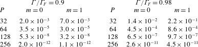
 $P\leqslant N_{S}$ accounts for a further truncation of the highly damped short waves, which have a negligible effect on the pilot-wave dynamics (but do play a role in the computation of the DtN map). Suitable values of
 $P\leqslant N_{S}$ are discussed in § B.2. We then solve the governing equations (2.13) numerically for a given vibrational forcing
 $\unicode[STIX]{x1D6E4}<\unicode[STIX]{x1D6E4}_{F}$ to find
 $\unicode[STIX]{x1D702}_{mp}(t_{1})$ and
 $\unicode[STIX]{x1D719}_{mp}(t_{1})$ (for all
 $p=1,\ldots ,P$), corresponding to the entries of
 $\unicode[STIX]{x1D648}_{m}\in \mathbb{R}^{2P\times 2P}$ for column number
 $(q+P\unicode[STIX]{x1D70D})$. The numerical integration is performed using a fourth-order Runge–Kutta method with the integrating factor
 $\exp (2Re^{-1}k_{mp}^{2}(t-\unicode[STIX]{x1D70F}_{j}))$ for integrating from time
 $t=\unicode[STIX]{x1D70F}_{j}$ to
 $t=\unicode[STIX]{x1D70F}_{j+1}$.
When truncating to  $P\leqslant N_{S}$ wavenumbers, we define vectors
 $\boldsymbol{\unicode[STIX]{x1D702}}_{m}^{n},\unicode[STIX]{x1D753}_{m}^{n}\in \mathbb{C}^{P\times 1}$ as
 $$\begin{eqnarray}\boldsymbol{\unicode[STIX]{x1D702}}_{m}^{n}=(\unicode[STIX]{x1D702}_{m1}(t_{n}),\ldots ,\unicode[STIX]{x1D702}_{mP}(t_{n}))^{\text{T}}\quad \text{and}\quad \unicode[STIX]{x1D753}_{m}^{n}=(\unicode[STIX]{x1D719}_{m1}(t_{n}^{+}),\ldots ,\unicode[STIX]{x1D719}_{mP}(t_{n}^{+}))^{\text{T}},\end{eqnarray}$$
where  $\unicode[STIX]{x1D702}$ is continuous across each impact, whereas we consider the velocity potential,
 $\unicode[STIX]{x1D719}$, in the instant just after impact. We also define
 $\unicode[STIX]{x1D64B}_{m}\in \mathbb{R}^{P\times P}$ as a diagonal matrix with elements
 $(2\unicode[STIX]{x03C0}C_{mp})^{-1}$ (the jump condition coefficients), and the row vector of basis functions
 $\unicode[STIX]{x1D731}_{m}(\boldsymbol{x})=(\unicode[STIX]{x1D6F7}_{m1}(\boldsymbol{x}),\ldots ,\unicode[STIX]{x1D6F7}_{mP}(\boldsymbol{x}))$. Combining the wave field evolution during flight (2.13) and at impact (2.12) yields (2.16b) in the iterative map below.
Under the imposed choice of  $f(t)=\sum _{n=0}^{\infty }\unicode[STIX]{x1D6FF}(t-t_{n})$, equation (2.3) may be decomposed into the droplet’s horizontal motion during flight (
 $t\neq t_{n}$)
 $$\begin{eqnarray}\boldsymbol{X}^{\prime \prime }(t)+C_{a}\boldsymbol{X}^{\prime }(t)=\mathbf{0},\end{eqnarray}$$
with jumps in the droplet’s horizontal velocity at impact (Durey & Milewski Reference Durey and Milewski2017)
 $$\begin{eqnarray}[\boldsymbol{X}^{\prime }(t_{n})]_{-}^{+}=-(1-\text{e}^{-C_{i}})\left(\frac{\unicode[STIX]{x1D6FF}_{0}G}{C_{i}}\unicode[STIX]{x1D735}\unicode[STIX]{x1D702}(\boldsymbol{X}(t_{n}),t_{n})+\boldsymbol{X}^{\prime }(t_{n}^{-})\right).\end{eqnarray}$$
To express the droplet dynamics (2.14)–(2.15) as a discrete-time map, we integrate (2.14) analytically and eliminate  $\boldsymbol{X}^{\prime }(t_{n}^{\pm })$ in (2.15) in favour of
 $\boldsymbol{X}(t_{n})$ and
 $\boldsymbol{X}(t_{n+1})$. Then, by defining
 $\boldsymbol{X}_{n}=\boldsymbol{X}(t_{n})$ as the droplet position at impact and
 $\boldsymbol{U}_{n}=\boldsymbol{X}_{n+1}-\boldsymbol{X}_{n}$ as the mean velocity during flight, the iterative map for the corral pilot-wave dynamics is
 $$\begin{eqnarray}\displaystyle & \displaystyle \boldsymbol{X}_{n}-\boldsymbol{X}_{n-1}=\boldsymbol{U}_{n-1}, & \displaystyle\end{eqnarray}$$
 $$\begin{eqnarray}\displaystyle & \displaystyle \left(\begin{array}{@{}c@{}}\boldsymbol{\unicode[STIX]{x1D702}}_{m}^{n}\\ \unicode[STIX]{x1D753}_{m}^{n}\end{array}\right)=\unicode[STIX]{x1D648}_{m}(\unicode[STIX]{x1D6E4})\left(\begin{array}{@{}c@{}}\boldsymbol{\unicode[STIX]{x1D702}}_{m}^{n-1}\\ \unicode[STIX]{x1D753}_{m}^{n-1}\end{array}\right)-\left(\begin{array}{@{}c@{}}\mathbf{0}\\ \unicode[STIX]{x1D64B}_{m}\unicode[STIX]{x1D731}_{m}^{\ast }(\boldsymbol{X}_{n})\end{array}\right), & \displaystyle\end{eqnarray}$$
 $$\begin{eqnarray}\displaystyle & \displaystyle (\boldsymbol{U}_{n}-\boldsymbol{U}_{n-1})+{\mathcal{D}}\boldsymbol{U}_{n-1}=-{\mathcal{F}}\unicode[STIX]{x1D735}\unicode[STIX]{x1D702}(\boldsymbol{X}_{n},t_{n}), & \displaystyle\end{eqnarray}$$
 $\ast$ denotes the matrix conjugate transpose, and the free surface is
 $\unicode[STIX]{x1D702}(\boldsymbol{x},t_{n})=\sum _{m=-\infty }^{\infty }\unicode[STIX]{x1D731}_{m}(\boldsymbol{x})\boldsymbol{\unicode[STIX]{x1D702}}_{m}^{n}$. Furthermore, the drag,
 ${\mathcal{D}}$, and wave force,
 ${\mathcal{F}}$, coefficients are
 $$\begin{eqnarray}{\mathcal{D}}=1-\text{e}^{-(C_{i}+C_{a})}\quad \text{and}\quad {\mathcal{F}}=\frac{1-\text{e}^{-C_{i}}}{C_{i}}\frac{1-\text{e}^{-C_{a}}}{C_{a}}\unicode[STIX]{x1D6FF}_{0}G.\end{eqnarray}$$
MATLAB code for evolving (2.16) is provided in the supplementary material.
2.4 Summary
In § 2, we derived a first-principles fluid model for the corral geometry, which is coupled to a reduced model for the droplet’s evolution. To recast this pilot-wave system into a tractable form, we formulated a method for numerically computing the DtN map for the corral geometry, reducing the evolution of the system to flow on the surface. As discussed in §§ 2.1 and 2.2, this methodology supersedes the ad hoc formulation of Faria (Reference Faria2017) in many respects. We then utilised fundamental matrices to express the evolution of the system as a discrete-time iterative map, where all the information of the corral geometry, vibrational forcing and fluid properties is encoded within the fundamental matrices  $\unicode[STIX]{x1D648}_{m}(\unicode[STIX]{x1D6E4})$. This discrete-time formulation is not only computationally more efficient (compared to repeatedly evolving the waves during flight (Faria Reference Faria2017)), but also provides a framework amenable for detailed analysis of the pilot-wave dynamics.
3 Properties of the Faraday problem and pilot-wave system
For our study of this pilot-wave system, we henceforth employ  $N_{S}=512$ collocation points with the further truncation to the first
 $P=128$ wavenumbers. We fix the corral dimensions as
 $R_{\infty }=64~\text{mm}$,
 $H_{S}=0.6~\text{mm}$ and
 $H_{D}=6.6~\text{mm}$, consistent with the experiments of Harris et al. (Reference Harris, Moukhtar, Fort, Couder and Bush2013). We will investigate the effect of changing the radius of the submerged step,
 $R_{c}$, the frequency of the vibrational forcing,
 $f_{0}$, and the dimensionless acceleration,
 $\unicode[STIX]{x1D6E4}$. Given
 $R_{\infty }$ and
 $N_{S}$, we restrict the corral radius to increments of
 $\unicode[STIX]{x0394}R_{c}=R_{\infty }/N_{S}=0.125~\text{mm}$. To incorporate regimes explored in prior experimental studies (Harris et al. Reference Harris, Moukhtar, Fort, Couder and Bush2013; Cristea-Platon et al. Reference Cristea-Platon, Sáenz and Bush2018; Sáenz et al. Reference Sáenz, Pucci, Goujon, Cristea-Platon and Bush2018), we consider
 $5\,\text{mm}\leqslant R_{c}\leqslant 15\,\text{mm}$. We note that Cristea-Platon et al. (Reference Cristea-Platon, Sáenz and Bush2018) instead used a shallow depth of
 $H_{S}=0.22~\text{mm}$, which is too shallow to be accurately described by quasi-potential flow.
3.1 The Faraday threshold
In addition to computational efficiency, the fundamental matrices,  $\unicode[STIX]{x1D648}_{m}(\unicode[STIX]{x1D6E4})$, also determine the subharmonic Faraday eigenmodes for given vibrational forcing
 $\unicode[STIX]{x1D6E4}<\unicode[STIX]{x1D6E4}_{F}$. Furthermore, the eigenvalues of
 $\unicode[STIX]{x1D648}_{m}$ give the decay rates of each fluid eigenmode. For each
 $m\in \mathbb{Z}$, we denote the dominant real eigenvalue as
 $\unicode[STIX]{x1D706}_{m}^{c}(\unicode[STIX]{x1D6E4})$, which satisfies
 $$\begin{eqnarray}\unicode[STIX]{x1D648}_{m}\left(\begin{array}{@{}c@{}}\boldsymbol{\unicode[STIX]{x1D702}}_{m}^{c}\\ \unicode[STIX]{x1D753}_{m}^{c}\end{array}\right)=\unicode[STIX]{x1D706}_{m}^{c}\left(\begin{array}{@{}c@{}}\boldsymbol{\unicode[STIX]{x1D702}}_{m}^{c}\\ \unicode[STIX]{x1D753}_{m}^{c}\end{array}\right).\end{eqnarray}$$
Each angular mode destabilises at the critical vibrational forcing  $\unicode[STIX]{x1D6E4}=\unicode[STIX]{x1D6E4}_{m}^{c}$, where
 $\unicode[STIX]{x1D706}_{m}^{c}(\unicode[STIX]{x1D6E4}_{m}^{c})=1$. This feature contrasts with earlier works (Durey & Milewski Reference Durey and Milewski2017), where the Faraday threshold was independent of the angular mode,
 $m$, for a fluid of infinite depth and horizontal extent. The corresponding Faraday threshold,
 $\unicode[STIX]{x1D6E4}_{F}$, for the corral geometry is thus the minimum for each angular mode, with
 $\unicode[STIX]{x1D6E4}_{F}=\min _{m}\unicode[STIX]{x1D6E4}_{m}^{c}.$ For
 $\unicode[STIX]{x1D6E4}<\unicode[STIX]{x1D6E4}_{m}^{c}$ and each angular mode
 $m$, the critical eigenvalue,
 $\unicode[STIX]{x1D706}_{m}^{c}(\unicode[STIX]{x1D6E4})$, determines the memory
 ${\mathcal{M}}_{m}(\unicode[STIX]{x1D6E4})=|\text{log}\,\unicode[STIX]{x1D706}_{m}^{c}(\unicode[STIX]{x1D6E4})|^{-1}$, a proxy for the number of prior impacts that significantly influence the system. The relative magnitude of each angular memory,
 ${\mathcal{M}}_{m}$, controls the form of the pilot-wave dynamics as
 $\unicode[STIX]{x1D6E4}\rightarrow \unicode[STIX]{x1D6E4}_{F}$, a concept revisited throughout this work. Moreover, the system memory,
 $Me(\unicode[STIX]{x1D6E4})=\max _{m}{\mathcal{M}}_{m}(\unicode[STIX]{x1D6E4})$, diverges in the limit
 $\unicode[STIX]{x1D6E4}\rightarrow \unicode[STIX]{x1D6E4}_{F}$.
3.2 Cavity modes
At the critical vibrational forcing  $\unicode[STIX]{x1D6E4}_{m}^{c}$ for each angular mode
 $m$, the eigenvalue problem (3.1) yields the Faraday cavity modes
 $\boldsymbol{\unicode[STIX]{x1D702}}_{m}^{c}$ and
 $\unicode[STIX]{x1D753}_{m}^{c}$. Inverting the Hankel transform back to physical space gives the corresponding radial part of each free-surface cavity mode, namely
 $\unicode[STIX]{x1D702}_{m}^{c}(r,t_{0})$ and
 $\unicode[STIX]{x1D719}_{m}^{c}(r,t_{0})$. It should be noted that, unlike the free-space dynamics explored in earlier works (Durey & Milewski Reference Durey and Milewski2017), the cavity modes are a superposition of Bessel functions with different wavenumbers. In particular, beyond the submerged step (
 $r\geqslant 1$), we observe exponential spatial decay in
 $\unicode[STIX]{x1D702}_{m}^{c}$ and
 $\unicode[STIX]{x1D719}_{m}^{c}$.
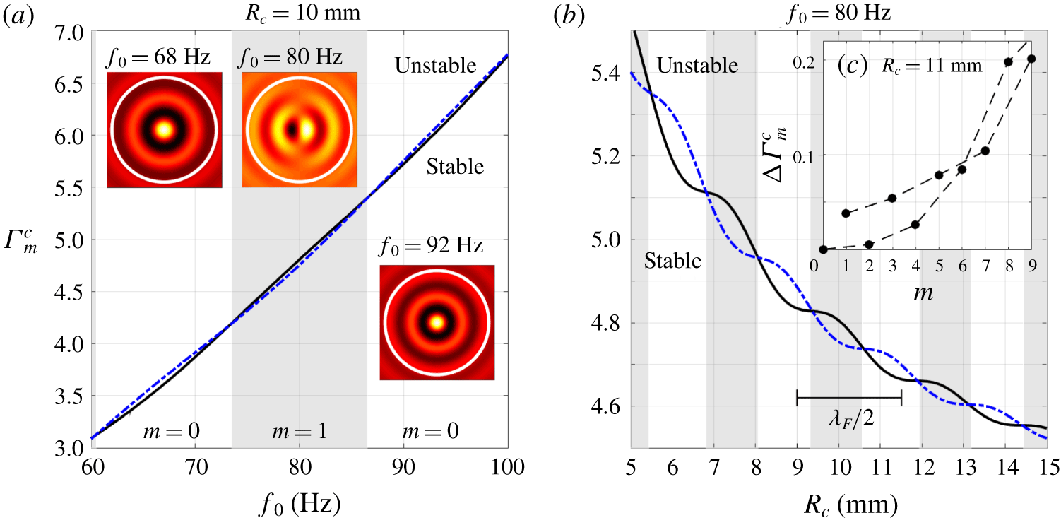
The critical vibrational forcing,  $\unicode[STIX]{x1D6E4}_{m}^{c}$, for
 $m=0$ (solid curve) and
 $m=1$ (dash-dotted curve), where the Faraday threshold is
 $\unicode[STIX]{x1D6E4}_{F}=\min _{m}\unicode[STIX]{x1D6E4}_{m}^{c}$. When
 $\unicode[STIX]{x1D6E4}_{0}^{c}<\unicode[STIX]{x1D6E4}_{1}^{c}$ (white background), the critical Faraday mode is axisymmetric, but has angular dependence for
 $\unicode[STIX]{x1D6E4}_{0}^{c}>\unicode[STIX]{x1D6E4}_{1}^{c}$ (grey background). (a) The dependence of
 $\unicode[STIX]{x1D6E4}_{m}^{c}$ on the vibrational frequency,
 $f_{0}$, for corral radius
 $R_{c}=10~\text{mm}$. The insets portray the real part of the critical cavity mode
 $\unicode[STIX]{x1D702}_{m}^{c}(r,0)\text{e}^{\text{i}m\unicode[STIX]{x1D703}}$ at
 $\unicode[STIX]{x1D6E4}=\unicode[STIX]{x1D6E4}_{m}^{c}=\unicode[STIX]{x1D6E4}_{F}$ for frequencies
 $f_{0}=68~\text{Hz}$,
 $f_{0}=80~\text{Hz}$ and
 $f_{0}=92~\text{Hz}$ (arbitrary vertical units). The white circle indicates the submerged step. (b) The dependence of
 $\unicode[STIX]{x1D6E4}_{m}^{c}$ on the corral radius,
 $R_{c}$, for frequency
 $f_{0}=80~\text{Hz}$. The marker indicates half the Faraday wavelength,
 $\unicode[STIX]{x1D706}_{F}=5.02~\text{mm}$, for a circular cylinder of constant depth
 $H_{D}=6.6~\text{mm}$ (Milewski et al. Reference Milewski, Galeano-Rios, Nachbin and Bush2015). (c) The increase in critical forcing,
 $\unicode[STIX]{x0394}\unicode[STIX]{x1D6E4}_{m}^{c}=\unicode[STIX]{x1D6E4}_{m}^{c}-\unicode[STIX]{x1D6E4}_{F}$, for corral radius
 $R_{c}=11~\text{mm}$ with frequency
 $f_{0}=80~\text{Hz}$, where
 $\unicode[STIX]{x1D6E4}_{F}=\unicode[STIX]{x1D6E4}_{0}^{c}$. The dashed lines are guides for the eyes.

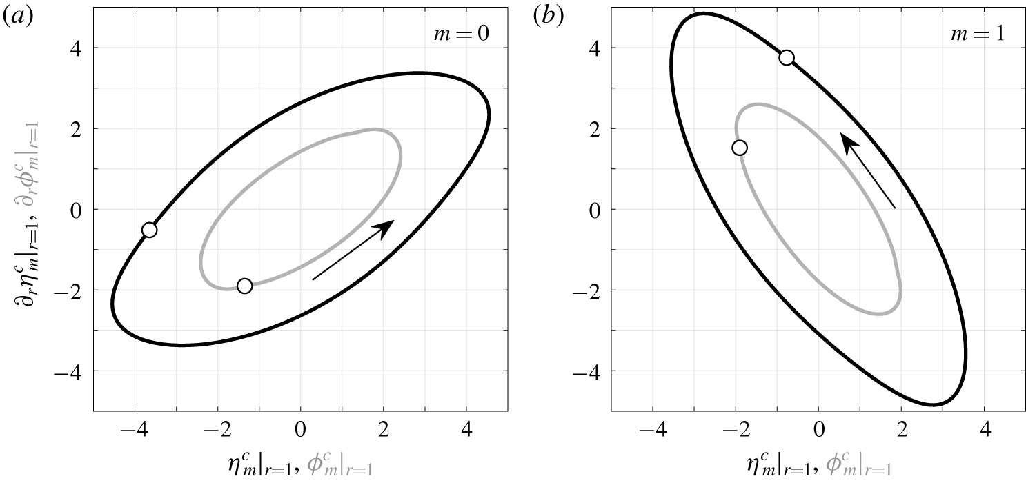
Phase-space time evolution of the dimensionless cavity modes  $\unicode[STIX]{x1D702}_{m}^{c}$ (black) and
 $\unicode[STIX]{x1D719}_{m}^{c}$ (grey) at
 $r=1$ (in arbitrary units). (a)
 $m=0$ and
 $\unicode[STIX]{x1D6E4}=\unicode[STIX]{x1D6E4}_{0}^{c}=4.806$, (b)
 $m=1$ and
 $\unicode[STIX]{x1D6E4}=\unicode[STIX]{x1D6E4}_{1}^{c}=4.754$. If a Dirichlet or Neumann approximation were adequate to describe the dynamics at
 $r=1$ then the trajectories would be approximately vertical or horizontal, respectively. The arrow denotes the time evolution. The reference dots denote the functions evaluated at time
 $t=0$. The frequency is
 $f_{0}=80~\text{Hz}$ with corral radius
 $R_{c}=10~\text{mm}$.

In figure 6, we present the critical vibrational forcing,  $\unicode[STIX]{x1D6E4}_{m}^{c}$, as a function of vibrational frequency,
 $f_{0}$, and corral radius,
 $R_{c}$. Not only does changing the forcing frequency affect the Faraday wavelength,
 $\unicode[STIX]{x1D706}_{F}$, and the subharmonic Faraday period,
 $T_{F}=2/f_{0}$, but it also determines which angular mode,
 $m$, is the most unstable, i.e. the value of
 $m$ that minimises the critical forcing acceleration,
 $\unicode[STIX]{x1D6E4}_{m}^{c}$. For
 $73.5\lesssim f_{0}\lesssim 86.5~\text{Hz}$, the
 $m=1$ mode is excited beyond the critical forcing acceleration, whereas there exist surrounding regions where the critical mode is radially symmetric (
 $m=0$). In the parameter regimes considered, we observed that
 $\unicode[STIX]{x1D6E4}_{2m}^{c}\geqslant \unicode[STIX]{x1D6E4}_{2m-2}^{c}$ and
 $\unicode[STIX]{x1D6E4}_{2m+1}^{c}\geqslant \unicode[STIX]{x1D6E4}_{2m-1}^{c}$ for all
 $m\geqslant 1$ (see figure 6c), indicating that the Faraday instability,
 $\unicode[STIX]{x1D6E4}_{F}$, corresponds only to cavity modes with radial symmetry (
 $m=0$) or the lowest angular frequency
 $(m=1)$. This result differs from the Faraday instability in a circular cylinder, where cavity modes with larger angular frequencies may be the first to destabilise (Gilet Reference Gilet2016). We note, however, that there is no guarantee that the supercritical Faraday pattern predicted by the linear theory will agree with experiments, for which weakly nonlinear (Skeldon & Rucklidge Reference Skeldon and Rucklidge2015) and fully nonlinear (Périnet, Juric & Tuckerman Reference Périnet, Juric and Tuckerman2009; Kahouadji et al. Reference Kahouadji, Périnet, Tuckerman, Shin, Chergui and Juric2015) effects will be significant. Nevertheless, when only one angular mode is linearly unstable, we may expect that the nonlinear Faraday pattern has a similar form for a supercritical bifurcation at the Faraday threshold. Finally, it is important to note that, for subcritical vibrational forcing (
 $\unicode[STIX]{x1D6E4}<\unicode[STIX]{x1D6E4}_{F}$), we do not observe any consistent ordering of the memories
 ${\mathcal{M}}_{m}$.
To explore the feasibility of a simple effective boundary condition above the step, we consider the time evolution of the amplitude and gradient of the cavity modes,  $\unicode[STIX]{x1D702}_{m}^{c}(r,t)$ and
 $\unicode[STIX]{x1D719}_{m}^{c}(r,t)$, evaluated at
 $r=1$, with the results presented in figure 7. At the critical vibrational forcing,
 $\unicode[STIX]{x1D6E4}_{m}^{c}$, the time evolution of the cavity modes is necessarily periodic, whereas the phase-space trajectory spirals towards the origin on the memory time scale,
 ${\mathcal{M}}_{m}$, for subcritical vibrations. Since the evolution of the free surface and velocity potential does not yield straight lines in phase space, considering effective Dirichlet (Blanchette Reference Blanchette2016; Filoux et al. Reference Filoux, Hubert, Schlagheck and Vandewalle2017), Neumann (Dubertrand et al. Reference Dubertrand, Hubert, Schlagheck, Vandewalle, Bastin and Martin2016; Gilet Reference Gilet2016) or Robin boundary conditions for
 $\unicode[STIX]{x1D702}_{m}^{c}$ and
 $\unicode[STIX]{x1D719}_{m}^{c}$ above the submerged step would be inadequate for capturing the evolution of the cavity modes. This result is an important feature of our study and highlights the benefits of our approach. A similar result was observed for the reflection of a walker off a submerged planar wall (Damiano et al. Reference Damiano, Brun, Harris, Galeano-Rios and Bush2016; Faria Reference Faria2017).
3.3 Relating the droplet statistics and the mean pilot wave
In certain circumstances, the mean pilot wave, averaged over the droplet’s trajectory, has a controlling influence on the droplet motion, determining the quantisation length of periodic trajectories (Labousse et al. Reference Labousse, Perrard, Couder and Fort2014; Perrard et al. Reference Perrard, Labousse, Miskin, Fort and Couder2014b) or acting as an effective potential in the long-path-memory limit (Cristea-Platon et al. Reference Cristea-Platon, Sáenz and Bush2018; Durey, Milewski & Bush Reference Durey, Milewski and Bush2018). Indeed, in an experimental study of elliptical corrals, Sáenz et al. (Reference Sáenz, Cristea-Platon and Bush2018) observed that the droplet’s statistical distribution and the accompanying mean pilot wave have a similar form, a result that we precisely define for the pilot-wave model considered herein.
As discussed by Durey et al. (Reference Durey, Milewski and Bush2018), several experimental and numerical studies provide evidence to support the validity of the ergodic hypothesis for confined, chaotic pilot-wave dynamics, typically leading to the emergence of a stationary probability density function,  $\unicode[STIX]{x1D707}(\boldsymbol{x})$, for the droplet’s position. Under the assumptions of ergodicity and stationarity, we prove in § C.1 that the mean wave field
 $$\begin{eqnarray}\bar{\unicode[STIX]{x1D702}}(\boldsymbol{x})=\lim _{N\rightarrow \infty }\frac{1}{N}\mathop{\sum }_{n=1}^{N}\unicode[STIX]{x1D702}(\boldsymbol{x},t_{n})\end{eqnarray}$$
satisfies
 $$\begin{eqnarray}\bar{\unicode[STIX]{x1D702}}(\boldsymbol{x})=\int _{\mathbb{R}^{2}}\unicode[STIX]{x1D702}_{G}(\boldsymbol{x};\boldsymbol{y})\unicode[STIX]{x1D707}(\,\boldsymbol{y})\,\text{d}\boldsymbol{y},\end{eqnarray}$$
where the wave field generated by infinitely many prior impacts at position  $\boldsymbol{x}=\boldsymbol{x}_{0}$ is
 $\unicode[STIX]{x1D702}_{G}(\boldsymbol{x};\boldsymbol{x}_{0})$, the time-periodic Green’s function for the domain (see figure 8 and appendix C for details). In contrast, the pilot-wave dynamics might instead be periodic, in which case
 $\boldsymbol{X}_{n+{\mathcal{P}}}=\boldsymbol{X}_{n}$ for all
 $n$ for some
 ${\mathcal{P}}\in \mathbb{N}$. As shown in § C.2, equation (3.2) also applies in this setting when we instead define
 $$\begin{eqnarray}\unicode[STIX]{x1D707}(\boldsymbol{x})=\frac{1}{{\mathcal{P}}}\mathop{\sum }_{n=1}^{{\mathcal{P}}}\unicode[STIX]{x1D6FF}(\boldsymbol{x}-\boldsymbol{X}_{n})\quad \text{and}\quad \bar{\unicode[STIX]{x1D702}}(\boldsymbol{x})=\frac{1}{{\mathcal{P}}}\mathop{\sum }_{n=1}^{{\mathcal{P}}}\unicode[STIX]{x1D702}(\boldsymbol{x},t_{n}).\end{eqnarray}$$
While we utilise these two relationships to elucidate the pilot-wave dynamics explored herein, there might also exist regimes in which the dynamics is neither ergodic nor periodic. One may then also consider the mean pilot wave generated over a finite time and its convergence to the asymptotic result given in (3.2). This statistical relaxation time was explored numerically by Tambasco & Bush (Reference Tambasco and Bush2018), where it was observed that the relaxation time scale was comparable to the memory time scale.
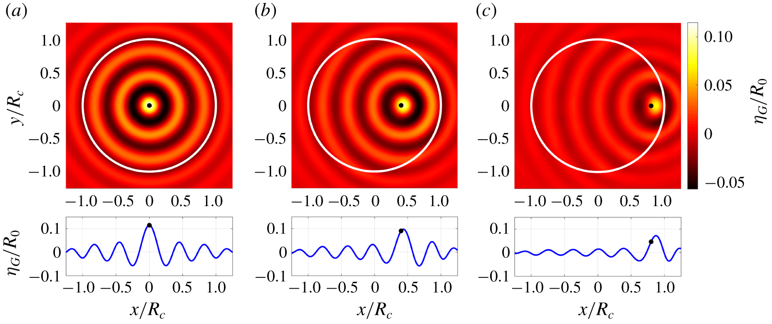
The wave field  $\unicode[STIX]{x1D702}_{G}(\boldsymbol{x};\boldsymbol{x}_{0})$ (upper panel) and its
 $y=0$ cross-section (lower panel). The white circles indicate the corral wall and the black dots denote the droplet position. We set
 $\boldsymbol{x}_{0}=(r_{0},0)^{\text{T}}$ with (a)
 $r_{0}=0$, (b)
 $r_{0}=0.4R_{c}$ and (c)
 $r_{0}=0.8R_{c}$. The corral radius is
 $R_{c}=14~\text{mm}$, with frequency
 $f_{0}=80~\text{Hz}$ and
 $\unicode[STIX]{x1D6E4}/\unicode[STIX]{x1D6E4}_{F}=0.965$, corresponding to memory
 $Me=19.3$. The droplet radius is
 $R_{0}=0.35~\text{mm}$ with impact phase
 $\unicode[STIX]{x1D703}_{I}=1.43\unicode[STIX]{x03C0}$. In the asymmetric cases, we observe three features of
 $\unicode[STIX]{x1D702}_{G}$: the magnitude of the wave decreases with
 $r_{0}$, the wave field gradient
 $\unicode[STIX]{x1D735}\unicode[STIX]{x1D702}_{G}$ is generally non-zero at
 $\boldsymbol{x}=\boldsymbol{x}_{0}$ (due to the wave reflection off the submerged step) and the wave damping increases in the shallow region, as is most apparent in (c).

To rationalise this observation for dynamics in a circular corral, we consider the pilot-wave dynamics arising on an initially quiescent bath. Moreover, by conditioning over the first  $N$ impacts of the droplet’s trajectory
 $\boldsymbol{X}_{0},\ldots ,\boldsymbol{X}_{N-1}$, we define the statistical distribution,
 $\unicode[STIX]{x1D707}_{N}(\boldsymbol{x})$, and accompanying mean wave field,
 $\bar{\unicode[STIX]{x1D702}}_{N}(\boldsymbol{x})$, as
 $$\begin{eqnarray}\unicode[STIX]{x1D707}_{N}(\boldsymbol{x})=\frac{1}{N}\mathop{\sum }_{n=0}^{N-1}\unicode[STIX]{x1D6FF}(\boldsymbol{x}-\boldsymbol{X}_{n})\quad \text{and}\quad \bar{\unicode[STIX]{x1D702}}_{N}(\boldsymbol{x})=\frac{1}{N}\mathop{\sum }_{n=0}^{N-1}\unicode[STIX]{x1D702}(\boldsymbol{x},t_{n}),\end{eqnarray}$$
respectively. As derived in § C.3, the trajectory-dependent mean pilot wave is  $\bar{\unicode[STIX]{x1D702}}_{N}(\boldsymbol{x})=\int _{\mathbb{R}^{2}}\unicode[STIX]{x1D702}_{G}(\boldsymbol{x};\boldsymbol{y})\unicode[STIX]{x1D707}_{N}(\,\boldsymbol{y})\,\text{d}\boldsymbol{y}+R_{N}(\boldsymbol{x})$, where the remainder term,
 $R_{N}(\boldsymbol{x})$, is
 $$\begin{eqnarray}R_{N}(\boldsymbol{x})=\frac{1}{N}\unicode[STIX]{x1D702}(\boldsymbol{x},t_{N-1})-\frac{1}{N}\mathop{\sum }_{m=-\infty }^{\infty }\left(\begin{array}{@{}cc@{}}\unicode[STIX]{x1D731}_{m}(\boldsymbol{x}) & \mathbf{0}\end{array}\right)(\unicode[STIX]{x1D644}-\unicode[STIX]{x1D648}_{m})^{-1}\left(\begin{array}{@{}c@{}}\boldsymbol{\unicode[STIX]{x1D702}}_{m}^{N-1}\\ \unicode[STIX]{x1D753}_{m}^{N-1}\end{array}\right).\end{eqnarray}$$
Strikingly, the remainder term,  $R_{N}(\boldsymbol{x})$, depends only on the wave field at the most recent impact. Assuming that the system remains bounded for all time, the first term decays to zero as
 $N\rightarrow \infty$ with size
 $O(1/N)$. As the dominant real eigenvalue of
 $(\unicode[STIX]{x1D644}-\unicode[STIX]{x1D648}_{m})^{-1}$ is
 ${\mathcal{M}}_{m}(1+O({\mathcal{M}}_{m}^{-1}))$ for
 ${\mathcal{M}}_{m}\gg 1$, and as
 $Me=\max _{m}{\mathcal{M}}_{m}$, we deduce that the second term in
 $R_{N}(\boldsymbol{x})$ has size
 $O(Me/N)$ as
 $N\rightarrow \infty$, rationalising the simulation results of Tambasco & Bush (Reference Tambasco and Bush2018). Moreover, the temporal decay of
 $R_{N}(\boldsymbol{x})$ highlights the robustness of the asymptotic relationship between
 $\bar{\unicode[STIX]{x1D702}}(\boldsymbol{x})$ and
 $\unicode[STIX]{x1D707}(\boldsymbol{x})$ given in (3.2).
3.4 The slow-moving limit: an effective potential
Cristea-Platon et al. (Reference Cristea-Platon, Sáenz and Bush2018) reported that when the droplet is confined to a corral, the pilot-wave system may exhibit a similar dynamics to the case where the droplet is instead subjected to a harmonic potential with no submerged topography (Perrard et al. Reference Perrard, Labousse, Fort and Couder2014a,Reference Perrard, Labousse, Miskin, Fort and Couderb). These two systems exhibit qualitatively different trapping mechanisms: in the case of an applied harmonic potential, the central force is applied directly to the droplet, whereas in a corral, the droplet is driven back towards the centre of the corral by the wave reflection off the submerged topography. To rationalise the origins of this similarity, we consider the form of the pilot wave for a droplet walking in the slow-moving limit. In this limit, the pilot wave at any given droplet position  $\boldsymbol{x}_{0}$ is well approximated by the wave field
 $\unicode[STIX]{x1D702}_{G}(\boldsymbol{x};\boldsymbol{x}_{0})$ of a stationary droplet bouncing at that same position (see figure 8). As the stationary droplet is positioned closer towards the submerged wall, the slope underneath the droplet deviates from zero, providing an inward radial force.
For a stationary bouncing at  $\boldsymbol{x}_{0}=r\boldsymbol{e}_{r}$, where
 $\boldsymbol{e}_{r}$ is a radial unit vector, the dimensionless inward force acting on the droplet is
 $F_{G}(r)=\boldsymbol{e}_{r}\boldsymbol{\cdot }\unicode[STIX]{x1D735}\unicode[STIX]{x1D702}_{G}(\boldsymbol{x};r\boldsymbol{e}_{r})|_{\boldsymbol{x}=r\boldsymbol{e}_{r}}$. An effective dimensionless potential,
 ${\mathcal{V}}(r)$, satisfies
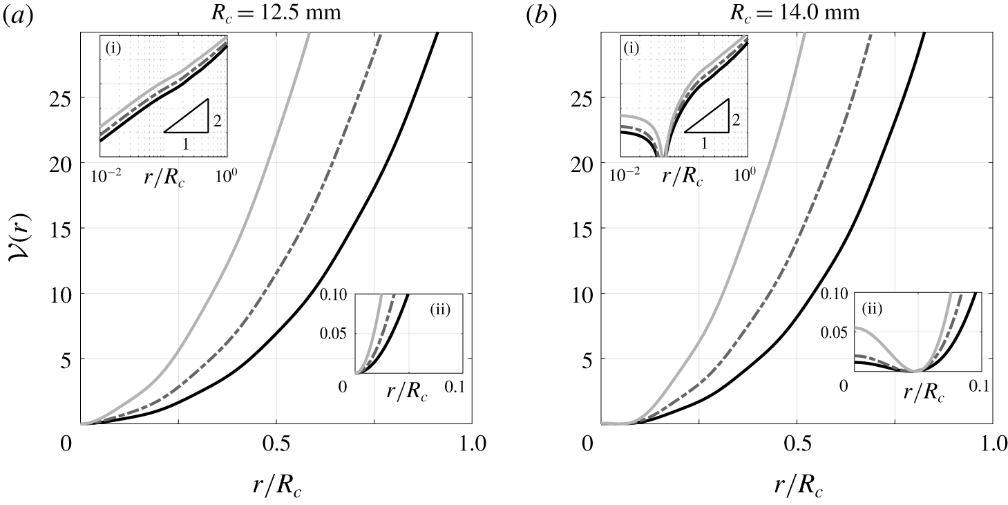
 ${\mathcal{V}}^{\prime }(r)=F_{G}(r)$. As presented in figure 9,
 ${\mathcal{V}}(r)$ is approximately quadratic in
 $r$ away from the origin, strikingly similar to a harmonic potential, suggesting a dynamical correspondence between these two systems in this particular limit. However, unlike an applied potential, the steepness of
 ${\mathcal{V}}(r)$ increases with the vibrational forcing and the origin is not always a minimum of the potential, as rationalised in § 4.3.
Dimensionless effective potential,  ${\mathcal{V}}(r)$, for a stationary droplet. The vibrational forcing is
 $\unicode[STIX]{x1D6E4}/\unicode[STIX]{x1D6E4}_{F}=0.80$ (black curve),
 $\unicode[STIX]{x1D6E4}/\unicode[STIX]{x1D6E4}_{F}=0.85$ (dash-dotted curve) and
 $\unicode[STIX]{x1D6E4}/\unicode[STIX]{x1D6E4}_{F}=0.90$ (light grey curve). (a)
 $R_{c}=12.5~\text{mm}$, (b)
 $R_{c}=14.0~\text{mm}$. Inset (i)
 ${\mathcal{V}}(r)$ for log–log axes, indicating quadratic-like growth away from the origin. Inset (ii)
 ${\mathcal{V}}(r)$ in the vicinity of the origin. The system parameters are
 $f_{0}=80~\text{Hz}$,
 $R_{0}=0.35~\text{mm}$ and
 $\unicode[STIX]{x1D703}_{I}=1.43\unicode[STIX]{x03C0}$.

3.5 Summary
In § 3, we explored the fundamental properties of this Faraday problem and pilot-wave system. We demonstrated that the form of the most unstable cavity mode depends on the corral geometry and the vibrational frequency. Furthermore, an effective boundary condition (in the form of a Dirichlet or Neumann condition above the step) is inadequate to describe the interaction with submerged topography, highlighting the limitations of prior works (Blanchette Reference Blanchette2016; Dubertrand et al. Reference Dubertrand, Hubert, Schlagheck, Vandewalle, Bastin and Martin2016; Gilet Reference Gilet2016; Filoux et al. Reference Filoux, Hubert, Schlagheck and Vandewalle2017). We then determined how the droplet statistics relate to the mean pilot wave, which may control the form of the pilot-wave dynamics in certain circumstances (Labousse et al. Reference Labousse, Perrard, Couder and Fort2014; Perrard et al. Reference Perrard, Labousse, Miskin, Fort and Couder2014b). Finally, we provided a rationale for the experimentally observed similitude between this corral system (Cristea-Platon et al. Reference Cristea-Platon, Sáenz and Bush2018) and the dynamics in a harmonic potential (Perrard et al. Reference Perrard, Labousse, Miskin, Fort and Couder2014b), demonstrating that the topography acts as a quadratic-like potential in the slow-moving limit. We proceed to explore the full range of pilot-wave dynamics predicted by this model, with the aim of rationalising further similarities and differences between the dynamics in a corral and a harmonic potential.
4 Stationary bouncing, circular orbits and the onset of quantisation
Following the experiments of Cristea-Platon et al. (Reference Cristea-Platon, Sáenz and Bush2018), we fix the vibrational frequency  $f_{0}=80~\text{Hz}$ and the droplet radius
 $R_{0}=0.35~\text{mm}$ for the remainder of this study. Although the impact phase,
 $\unicode[STIX]{x1D703}_{I}$, may vary weakly with the vibrational forcing (Moláček & Bush Reference Moláček and Bush2013), we henceforth fix
 $\unicode[STIX]{x1D703}_{I}=1.43\unicode[STIX]{x03C0}$, yielding free-walking speeds consistent with experiments. The particular value of
 $\unicode[STIX]{x1D703}_{I}$ does not change the qualitative features of the pilot-wave system: As
 $\unicode[STIX]{x1D703}_{I}$ is decreased towards
 $\unicode[STIX]{x03C0}$, the magnitude of the waves increases, decreasing the critical vibrational forcing at which instabilities arise.
To rationalise the dynamics of periodic bouncing and circular orbits, we express the iterative map (2.16) in a rotating frame of reference, prescribed by the (as yet unknown) orbital angular velocity,  $\unicode[STIX]{x1D703}_{0}$. Stationary bouncing corresponds to the special case
 $\unicode[STIX]{x1D703}_{0}=0$. By denoting the standard rotation matrix as
 $\unicode[STIX]{x1D64D}(\unicode[STIX]{x1D703}_{0})\in \mathbb{R}^{2\times 2}$, equation (2.16) is recast as
 $$\begin{eqnarray}\displaystyle & \displaystyle \left(\begin{array}{@{}c@{}}\boldsymbol{\unicode[STIX]{x1D702}}_{m}^{n}\\ \unicode[STIX]{x1D753}_{m}^{n}\end{array}\right)=\text{e}^{\text{i}m\unicode[STIX]{x1D703}_{0}}\unicode[STIX]{x1D648}_{m}\left(\begin{array}{@{}c@{}}\boldsymbol{\unicode[STIX]{x1D702}}_{m}^{n-1}\\ \unicode[STIX]{x1D753}_{m}^{n-1}\end{array}\right)-\left(\begin{array}{@{}c@{}}\mathbf{0}\\ \unicode[STIX]{x1D64B}_{m}\unicode[STIX]{x1D731}_{m}^{\ast }(\boldsymbol{X}_{n})\end{array}\right), & \displaystyle\end{eqnarray}$$
 $$\begin{eqnarray}\displaystyle & \displaystyle \unicode[STIX]{x1D64D}(\unicode[STIX]{x1D703}_{0})\boldsymbol{X}_{n+1}-2\boldsymbol{X}_{n}+\unicode[STIX]{x1D64D}(-\unicode[STIX]{x1D703}_{0})\boldsymbol{X}_{n-1}=-{\mathcal{D}}(\boldsymbol{X}_{n}-\unicode[STIX]{x1D64D}(-\unicode[STIX]{x1D703}_{0})\boldsymbol{X}_{n-1})-{\mathcal{F}}\unicode[STIX]{x1D735}\unicode[STIX]{x1D702}(\boldsymbol{X}_{n},t_{n}).\quad & \displaystyle\end{eqnarray}$$
We now seek a fixed point of (4.1) corresponding to a circular orbit of radius  $r_{0}>0$ with dimensionless angular velocity
 $\unicode[STIX]{x1D703}_{0}$. Hence,
 $\boldsymbol{X}_{n}=r_{0}\boldsymbol{e}_{r}$ for all
 $n$, where
 $\boldsymbol{e}_{r}=(\cos \unicode[STIX]{x1D6FC},\sin \unicode[STIX]{x1D6FC})^{\text{T}}$ is a fixed arbitrary unit vector (
 $\unicode[STIX]{x1D6FC}\in \mathbb{R}$), with corresponding wave field coefficients
 $\boldsymbol{\unicode[STIX]{x1D702}}_{m}^{n}=\boldsymbol{\unicode[STIX]{x1D702}}_{m}^{O}$ and
 $\unicode[STIX]{x1D753}_{m}^{n}=\unicode[STIX]{x1D753}_{m}^{O}$ for all
 $n$. Substituting this orbital ansatz into (4.1) yields
 $$\begin{eqnarray}\displaystyle & \displaystyle (\unicode[STIX]{x1D644}-\text{e}^{\text{i}m\unicode[STIX]{x1D703}_{0}}\unicode[STIX]{x1D648}_{m})\left(\begin{array}{@{}c@{}}\boldsymbol{\unicode[STIX]{x1D702}}_{m}^{O}\\ \unicode[STIX]{x1D753}_{m}^{O}\end{array}\right)=-\left(\begin{array}{@{}c@{}}\mathbf{0}\\ \unicode[STIX]{x1D64B}_{m}\unicode[STIX]{x1D731}_{m}^{\ast }(r_{0}\boldsymbol{ e}_{r})\end{array}\right), & \displaystyle\end{eqnarray}$$
 $$\begin{eqnarray}\displaystyle & \displaystyle (\unicode[STIX]{x1D64D}(\unicode[STIX]{x1D703}_{0})-2\unicode[STIX]{x1D644}+\unicode[STIX]{x1D64D}(-\unicode[STIX]{x1D703}_{0})+{\mathcal{D}}(\unicode[STIX]{x1D644}-\unicode[STIX]{x1D64D}(-\unicode[STIX]{x1D703}_{0})))r_{0}\boldsymbol{e}_{r}=-{\mathcal{F}}\unicode[STIX]{x1D735}\unicode[STIX]{x1D702}_{O}(r_{0}\boldsymbol{e}_{r}), & \displaystyle\end{eqnarray}$$
 $\unicode[STIX]{x1D702}_{O}(\boldsymbol{x})=\sum _{m=-\infty }^{\infty }\unicode[STIX]{x1D731}_{m}(\boldsymbol{x})\boldsymbol{\unicode[STIX]{x1D702}}_{m}^{O}$ is the corresponding orbital wave field. By solving (4.2a) for
 $\boldsymbol{\unicode[STIX]{x1D702}}_{m}^{O}$ and defining the Jacobian matrix
 $$\begin{eqnarray}\unicode[STIX]{x1D645}_{m}(\boldsymbol{x})=\left(\begin{array}{@{}c@{}}\unicode[STIX]{x2202}_{x}\unicode[STIX]{x1D731}_{m}(\boldsymbol{x})\\ \unicode[STIX]{x2202}_{y}\unicode[STIX]{x1D731}_{m}(\boldsymbol{x})\end{array}\right),\end{eqnarray}$$
we obtain
 $$\begin{eqnarray}\unicode[STIX]{x1D735}\unicode[STIX]{x1D702}_{O}(r_{0}\boldsymbol{ e}_{r})=-\mathop{\sum }_{m=-\infty }^{\infty }\left(\begin{array}{@{}cc@{}}\unicode[STIX]{x1D645}_{m}(r_{0}\boldsymbol{e}_{r}) & \unicode[STIX]{x1D7EC}\end{array}\right)(\unicode[STIX]{x1D644}-\text{e}^{\text{i}m\unicode[STIX]{x1D703}_{0}}\unicode[STIX]{x1D648}_{m})^{-1}\left(\begin{array}{@{}c@{}}\mathbf{0}\\ \unicode[STIX]{x1D64B}_{m}\unicode[STIX]{x1D731}_{m}^{\ast }(r_{0}\boldsymbol{e}_{r})\end{array}\right).\end{eqnarray}$$
Furthermore, rearranging the droplet equation (4.2b) yields
 $$\begin{eqnarray}({\mathcal{D}}-2)(1-\cos \unicode[STIX]{x1D703}_{0})r_{0}\boldsymbol{e}_{r}+{\mathcal{D}}r_{0}\sin \unicode[STIX]{x1D703}_{0}\boldsymbol{e}_{\unicode[STIX]{x1D703}}=-{\mathcal{F}}\unicode[STIX]{x1D735}\unicode[STIX]{x1D702}_{O}(r_{0}\boldsymbol{e}_{r}),\end{eqnarray}$$
where the unit vector  $\boldsymbol{e}_{\unicode[STIX]{x1D703}}=(-\!\sin \unicode[STIX]{x1D6FC},\cos \unicode[STIX]{x1D6FC})^{\text{T}}$ is orthogonal to
 $\boldsymbol{e}_{r}$. By combining (4.3)–(4.4), we seek
 $r_{0}>0$ and
 $\unicode[STIX]{x1D703}_{0}\in \mathbb{R}$ for given
 $\unicode[STIX]{x1D6E4}<\unicode[STIX]{x1D6E4}_{F}$ such that
 $$\begin{eqnarray}\displaystyle & & \displaystyle ({\mathcal{D}}-2)(1-\cos \unicode[STIX]{x1D703}_{0})r_{0}\boldsymbol{e}_{r}+{\mathcal{D}}r_{0}\sin \unicode[STIX]{x1D703}_{0}\boldsymbol{e}_{\unicode[STIX]{x1D703}}\nonumber\\ \displaystyle & & \displaystyle \quad ={\mathcal{F}}\mathop{\sum }_{m=-\infty }^{\infty }\left(\begin{array}{@{}cc@{}}\unicode[STIX]{x1D645}_{m}(r_{0}\boldsymbol{e}_{r}) & \unicode[STIX]{x1D7EC}\end{array}\right)(\unicode[STIX]{x1D644}-\text{e}^{\text{i}m\unicode[STIX]{x1D703}_{0}}\unicode[STIX]{x1D648}_{m}(\unicode[STIX]{x1D6E4}))^{-1}\left(\begin{array}{@{}c@{}}\mathbf{0}\\ \unicode[STIX]{x1D64B}_{m}\unicode[STIX]{x1D731}_{m}^{\ast }(r_{0}\boldsymbol{e}_{r})\end{array}\right).\nonumber\end{eqnarray}$$
If  $(r_{0},\unicode[STIX]{x1D703}_{0})$ is a solution then so is
 $(r_{0},-\unicode[STIX]{x1D703}_{0})$, corresponding orbiting in the opposite direction. The dimensionless orbital speed is
 $u=2r_{0}|\text{sin}(\unicode[STIX]{x1D703}_{0}/2)|\approx r_{0}|\unicode[STIX]{x1D703}_{0}|$ for
 $|\unicode[STIX]{x1D703}_{0}|\ll 1$.
Orbiting ( $u>0$, solid curves) and bouncing (
 $u=0$, dotted curves) states for (a)
 $R_{c}=12.5~\text{mm}$ and (b)
 $R_{c}=14.0~\text{mm}$. We categorise the linear stability as follows: stable states (blue); unstable states with all unstable eigenvalues appearing in complex-conjugate pairs (green); there exists a real unstable eigenvalue (red). The white diamonds in (a) correspond to the orbital wave fields in figure 11. In both panels, the black circles denote the computed values of
 $r_{\ast }$ in the limit
 $\unicode[STIX]{x1D6E4}\rightarrow \unicode[STIX]{x1D6E4}_{F}$. The left inset in each panel denotes the form of the cavity mode at the Faraday threshold,
 $\unicode[STIX]{x1D6E4}=\unicode[STIX]{x1D6E4}_{F}$, where the critical mode is (a)
 $m=1$ and (b)
 $m=0$ (arbitrary vertical units). The right inset in each panel portrays the orbital speed,
 $u$. When multiple orbits exist at high memory, the speed lies in the range
 $8{-}10~\text{mm}~\text{s}^{-1}$. (a) The orbiting state bifurcates from stationary bouncing at the origin. (b) The orbiting state instead bifurcates from stationary bouncing a distance
 $r_{b}>0$ from the origin. The corresponding axisymmetric bouncing state is unstable for all
 $\unicode[STIX]{x1D6E4}<\unicode[STIX]{x1D6E4}_{F}$ in this case.

The orbital wave field,  $\unicode[STIX]{x1D702}_{O}$, for anticlockwise (
 $\unicode[STIX]{x1D703}_{0}>0$) orbital states denoted by the white diamonds in figure 10(a). (a)
 $\unicode[STIX]{x1D6E4}/\unicode[STIX]{x1D6E4}_{F}=0.86$,
 $r_{0}=0.12R_{c}$ and orbital speed
 $u=1.99~\text{mm}~\text{s}^{-1}$. (b)
 $\unicode[STIX]{x1D6E4}/\unicode[STIX]{x1D6E4}_{F}=0.90$,
 $r_{0}=0.32R_{c}$ and
 $u=6.00~\text{mm}~\text{s}^{-1}$. (c)
 $\unicode[STIX]{x1D6E4}/\unicode[STIX]{x1D6E4}_{F}=0.97$,
 $r_{0}=0.40R_{c}$ and
 $u=8.96~\text{mm}~\text{s}^{-1}$. All three orbits are stable according to the asymptotic linear stability analysis. The free-surface elevation is normalised by the droplet radius,
 $R_{0}=0.35~\text{mm}$. The droplet’s position and trajectory are marked by the black dot and dashed circle, respectively. The white circle denotes the submerged step.

Orbital solutions are presented in figure 10 for corral radii  $R_{c}=12.5~\text{mm}$ and
 $R_{c}=14~\text{mm}$. Asymptotic linear stability analysis (as derived in § 4.1) reveals that stable stationary bouncing states (with
 $u=0$) destabilise into circular orbits, which are typically stable for short path memory. As the influence of the droplet’s wake becomes more pronounced, circular orbits destabilise via a pair of complex-conjugate eigenvalues, yielding stable precessing loops (see § 5). In the long-path-memory limit, several quantised orbital solutions emerge (all of which are unstable), whose radii we rationalise in § 4.2. Finally, the bifurcation between bouncing and orbiting is qualitatively different in the cases
 $R_{c}=12.5~\text{mm}$ and
 $R_{c}=14~\text{mm}$. For
 $R_{c}=12.5~\text{mm}$, circular orbits bifurcate from the axisymmetric bouncing state, yet for
 $R_{c}=14~\text{mm}$, the circular orbits instead bifurcate from an off-centre bouncing state. We study this bifurcation and the existence of off-centre bouncing states in § 4.3. Simulations reveal that in the region of unstable, small-radius circular orbits (for
 $R_{c}=14~\text{mm}$ and
 $\unicode[STIX]{x1D6E4}\approx 0.86$), stable, small-amplitude rectilinear oscillations arise, akin to experiments (Cristea-Platon et al. Reference Cristea-Platon, Sáenz and Bush2018).
We present the orbital wave field,  $\unicode[STIX]{x1D702}_{O}(\boldsymbol{x})$, for three stable circular orbits (for
 $R_{c}=12.5~\text{mm}$) in figure 11. For short path memory (
 $\unicode[STIX]{x1D6E4}/\unicode[STIX]{x1D6E4}_{F}=0.86$), the orbital wave field has a similar form to the wave field of a droplet bouncing at the origin (see figure 8). However, as the vibrational forcing increases, the combined effect of increased orbital speed and longer path-memory results in a pronounced distortion of the droplet’s wake.
4.1 Linear stability analysis
To study the asymptotic linear stability of the orbital and bouncing states, we consider perturbations from the steady state of the form
 $$\begin{eqnarray}\boldsymbol{X}_{n}=r_{0}\boldsymbol{e}_{r}+\unicode[STIX]{x1D716}\hat{\boldsymbol{X}}_{n},\quad \boldsymbol{\unicode[STIX]{x1D702}}_{m}^{n}=\boldsymbol{\unicode[STIX]{x1D702}}_{m}^{O}+\unicode[STIX]{x1D716}\hat{\boldsymbol{\unicode[STIX]{x1D702}}}_{m}^{n},\quad \unicode[STIX]{x1D753}_{m}^{n}=\unicode[STIX]{x1D753}_{m}^{O}+\unicode[STIX]{x1D716}\hat{\unicode[STIX]{x1D753}}_{m}^{n},\end{eqnarray}$$
where  $0<\unicode[STIX]{x1D716}\ll 1$. Consequentially, the perturbed free surface at each impact is
 $\hat{\unicode[STIX]{x1D702}}(\boldsymbol{x},t_{n})=\sum _{m=-\infty }^{\infty }\unicode[STIX]{x1D731}_{m}(\boldsymbol{x})\hat{\boldsymbol{\unicode[STIX]{x1D702}}}_{m}^{n}$. By substituting this perturbation ansatz in the orbital trajectory equation (4.1), the perturbed variables evolve according to the linearised system
 $$\begin{eqnarray}\displaystyle & \displaystyle \left(\begin{array}{@{}c@{}}\hat{\boldsymbol{\unicode[STIX]{x1D702}}}_{m}^{n}\\ \hat{\unicode[STIX]{x1D753}}_{m}^{n}\end{array}\right)=\text{e}^{\text{i}m\unicode[STIX]{x1D703}_{0}}\unicode[STIX]{x1D648}_{m}\left(\begin{array}{@{}c@{}}\hat{\boldsymbol{\unicode[STIX]{x1D702}}}_{m}^{n-1}\\ \hat{\unicode[STIX]{x1D753}}_{m}^{n-1}\end{array}\right)-\left(\begin{array}{@{}c@{}}\mathbf{0}\\ \unicode[STIX]{x1D64B}_{m}\unicode[STIX]{x1D645}_{m}^{\ast }(r_{0}\boldsymbol{ e}_{r})\hat{\boldsymbol{X}}_{n}\end{array}\right), & \displaystyle\end{eqnarray}$$
 $$\begin{eqnarray}\displaystyle & \displaystyle \unicode[STIX]{x1D64D}_{+}\hat{\boldsymbol{X}}_{n+1}-2\hat{\boldsymbol{X}}_{n}+\unicode[STIX]{x1D64D}_{-}\hat{\boldsymbol{X}}_{n-1}=-{\mathcal{D}}(\hat{\boldsymbol{X}}_{n}-\unicode[STIX]{x1D64D}_{-}\hat{\boldsymbol{X}}_{n-1})-{\mathcal{F}}[\unicode[STIX]{x1D643}\hat{\boldsymbol{X}}_{n}+\unicode[STIX]{x1D735}\hat{\unicode[STIX]{x1D702}}(r_{0}\boldsymbol{e}_{r},t_{n})], & \displaystyle\end{eqnarray}$$
 $\unicode[STIX]{x1D64D}_{\pm }=\unicode[STIX]{x1D64D}(\pm \unicode[STIX]{x1D703}_{0})$ and
 $\unicode[STIX]{x1D643}$ is the Hessian matrix of the steady-state wave field,
 $\unicode[STIX]{x1D702}_{O}(\boldsymbol{x})$, evaluated at
 $\boldsymbol{x}=r_{0}\boldsymbol{e}_{r}$, namely
 $\unicode[STIX]{x1D643}=\unicode[STIX]{x1D735}\unicode[STIX]{x1D735}^{\text{T}}\unicode[STIX]{x1D702}_{O}(r_{0}\boldsymbol{e}_{r})$.
We now seek solutions to (4.5) where the perturbed variables evolve according to  $\hat{\boldsymbol{X}}_{n}=\unicode[STIX]{x1D706}^{n}\hat{\boldsymbol{X}}_{0}$,
 $\hat{\boldsymbol{\unicode[STIX]{x1D702}}}_{m}^{n}=\unicode[STIX]{x1D706}^{n}\hat{\boldsymbol{\unicode[STIX]{x1D702}}}_{m}^{0}$ and
 $\hat{\unicode[STIX]{x1D753}}_{m}^{n}=\unicode[STIX]{x1D706}^{n}\hat{\unicode[STIX]{x1D753}}_{m}^{0}$ for all
 $n$, where
 $\unicode[STIX]{x1D706}\in \mathbb{C}$ is an eigenvalue of the perturbed system (to be determined). By substituting this ansatz into (4.5), we obtain
 $$\begin{eqnarray}\displaystyle & \displaystyle (\unicode[STIX]{x1D706}\unicode[STIX]{x1D644}-\text{e}^{\text{i}m\unicode[STIX]{x1D703}_{0}}\unicode[STIX]{x1D648}_{m})\left(\begin{array}{@{}c@{}}\hat{\boldsymbol{\unicode[STIX]{x1D702}}}_{m}^{0}\\ \hat{\unicode[STIX]{x1D753}}_{m}^{0}\end{array}\right)=-\unicode[STIX]{x1D706}\left(\begin{array}{@{}c@{}}\unicode[STIX]{x1D7EC}\\ \unicode[STIX]{x1D64B}_{m}\unicode[STIX]{x1D645}_{m}^{\ast }(r_{0}\boldsymbol{e}_{r})\end{array}\right)\hat{\boldsymbol{X}}_{0}, & \displaystyle\end{eqnarray}$$
 $$\begin{eqnarray}\displaystyle & \displaystyle (\unicode[STIX]{x1D706}^{2}\unicode[STIX]{x1D64D}_{+}-2\unicode[STIX]{x1D706}\unicode[STIX]{x1D644}+\unicode[STIX]{x1D64D}_{-})\hat{\boldsymbol{X}}_{0}=-{\mathcal{D}}(\unicode[STIX]{x1D706}\unicode[STIX]{x1D644}-\unicode[STIX]{x1D64D}_{-})\hat{\boldsymbol{X}}_{0}-{\mathcal{F}}\unicode[STIX]{x1D706}[\unicode[STIX]{x1D643}\hat{\boldsymbol{X}}_{0}+\unicode[STIX]{x1D735}\hat{\unicode[STIX]{x1D702}}(r_{0}\boldsymbol{e}_{r},t_{0})]. & \displaystyle\end{eqnarray}$$
 $\unicode[STIX]{x1D735}\hat{\unicode[STIX]{x1D702}}(r_{0}\boldsymbol{e}_{r},t_{0})=-\unicode[STIX]{x1D706}\unicode[STIX]{x1D642}(\unicode[STIX]{x1D706})\hat{\boldsymbol{X}}_{0}$, where
 $\unicode[STIX]{x1D642}\in \mathbb{C}^{2\times 2}$ is defined as
 $$\begin{eqnarray}\unicode[STIX]{x1D642}(\unicode[STIX]{x1D706})=\mathop{\sum }_{m=-\infty }^{\infty }\left(\begin{array}{@{}cc@{}}\unicode[STIX]{x1D645}_{m}(r_{0}\boldsymbol{e}_{r}) & \unicode[STIX]{x1D7EC}\end{array}\right)(\unicode[STIX]{x1D706}\unicode[STIX]{x1D644}-\text{e}^{\text{i}m\unicode[STIX]{x1D703}_{0}}\unicode[STIX]{x1D648}_{m})^{-1}\left(\begin{array}{@{}c@{}}\unicode[STIX]{x1D7EC}\\ \unicode[STIX]{x1D64B}_{m}\unicode[STIX]{x1D645}_{m}^{\ast }(r_{0}\boldsymbol{e}_{r})\end{array}\right).\end{eqnarray}$$
Substituting  $\unicode[STIX]{x1D735}\hat{\unicode[STIX]{x1D702}}(r_{0}\boldsymbol{e}_{r},t_{0})$ into (4.6b) yields
 $\unicode[STIX]{x1D63C}(\unicode[STIX]{x1D706})\unicode[STIX]{x1D64D}_{-}\hat{\boldsymbol{X}}_{0}=\mathbf{0}$, where
 $$\begin{eqnarray}\unicode[STIX]{x1D63C}(\unicode[STIX]{x1D706})=(\unicode[STIX]{x1D706}\unicode[STIX]{x1D64D}_{+}-\unicode[STIX]{x1D644})^{2}+{\mathcal{D}}(\unicode[STIX]{x1D706}\unicode[STIX]{x1D64D}_{+}-\unicode[STIX]{x1D644})+\unicode[STIX]{x1D706}{\mathcal{F}}(\unicode[STIX]{x1D643}-\unicode[STIX]{x1D706}\unicode[STIX]{x1D642}(\unicode[STIX]{x1D706}))\unicode[STIX]{x1D64D}_{+}.\end{eqnarray}$$
For non-trivial  $\hat{\boldsymbol{X}}_{0}$, it remains to find an eigenvalue
 $\unicode[STIX]{x1D706}\in \mathbb{C}$ such that
 $\det \unicode[STIX]{x1D63C}(\unicode[STIX]{x1D706})=0$. The system is unstable if there exists
 $\unicode[STIX]{x1D706}$ such that
 $|\unicode[STIX]{x1D706}|>1$, and stable otherwise, where we note that rotational invariance (for
 $r_{0}>0$) supplies that
 $\unicode[STIX]{x1D706}=1$ is always an eigenvalue.
4.2 The high-memory limit: rationalising the orbital quantisation
The mean wave field,  $\bar{\unicode[STIX]{x1D702}}(\boldsymbol{x})$, associated with a circular orbit with radius
 $r_{0}$ is
 $$\begin{eqnarray}\bar{\unicode[STIX]{x1D702}}(\boldsymbol{x})=-\left(\begin{array}{@{}cc@{}}\unicode[STIX]{x1D731}_{0}(\boldsymbol{x}) & \mathbf{0}\end{array}\right)(\unicode[STIX]{x1D644}-\unicode[STIX]{x1D648}_{0})^{-1}\left(\begin{array}{@{}c@{}}\mathbf{0}\\ \unicode[STIX]{x1D64B}_{0}\unicode[STIX]{x1D731}_{0}^{\ast }(r_{0}\boldsymbol{e}_{r})\end{array}\right),\end{eqnarray}$$
which is exactly equal to the radially symmetric contribution to the orbital wave field,  $\unicode[STIX]{x1D702}_{O}(\boldsymbol{x})$, at each impact (see (4.2a)). Hence, the contribution of the mean wave field to the inward radial kick imparted on the droplet at each impact is defined as
 $F_{O}(r_{0})=\boldsymbol{e}_{r}\boldsymbol{\cdot }\unicode[STIX]{x1D735}\bar{\unicode[STIX]{x1D702}}(r_{0}\boldsymbol{e}_{r})$, where the function
 $F_{O}(r)$ is given by
 $$\begin{eqnarray}F_{O}(r)=-\boldsymbol{e}_{r}\boldsymbol{\cdot }\left(\begin{array}{@{}cc@{}}\unicode[STIX]{x1D645}_{0}(r\boldsymbol{e}_{r}) & \unicode[STIX]{x1D7EC}\end{array}\right)(\unicode[STIX]{x1D644}-\unicode[STIX]{x1D648}_{0})^{-1}\left(\begin{array}{@{}c@{}}\mathbf{0}\\ \unicode[STIX]{x1D64B}_{0}\unicode[STIX]{x1D731}_{0}^{\ast }(r\boldsymbol{e}_{r})\end{array}\right).\end{eqnarray}$$
We now use (4.8) to rationalise the emergence of orbital quantisation in the high-memory limit. We first consider the case where the  $m=0$ mode destabilises first (so
 $\unicode[STIX]{x1D6E4}_{F}=\unicode[STIX]{x1D6E4}_{0}^{c}$ and
 $Me={\mathcal{M}}_{0}$ close to the Faraday threshold). In the limit
 $\unicode[STIX]{x1D6E4}\rightarrow \unicode[STIX]{x1D6E4}_{F}$, the dominant real eigenvalue of
 $(\unicode[STIX]{x1D644}-\unicode[STIX]{x1D648}_{0})^{-1}$ is
 $Me(1+O(Me^{-1}))$ for
 $Me\gg 1$. Hence, the magnitude of the radial kick,
 $|F_{O}(r_{0})|$, grows without bound as
 $Me\rightarrow \infty$ unless the orbital radius,
 $r_{0}$, suppresses the singularity. This behaviour may be achieved via two different mechanisms: either the orbital radius,
 $r_{0}$, minimises the excitation of the radially symmetric mode, or the radially symmetric mode is excited at each impact yet
 $r_{0}$ lies at a radial extremum. Hence, in the case of an axisymmetric Faraday instability, the origin of orbital quantisation in a corral is analogous to dynamics in an unbounded domain: the corresponding expression for (4.8) in the limit
 $Me\rightarrow \infty$ may be approximated as
 $F_{O}(r)/Me\propto \text{J}_{0}(k_{F}r)\text{J}_{0}^{\prime }(k_{F}r)$, where
 $k_{F}$ is the critical Faraday wavenumber (Oza et al. Reference Oza, Harris, Rosales and Bush2014; Perrard et al. Reference Perrard, Labousse, Miskin, Fort and Couder2014b). Moreover, this quantisation mechanism depends on the droplet properties only through the impact phase,
 $\unicode[STIX]{x1D703}_{I}$, and is independent of
 ${\mathcal{D}}$ and
 ${\mathcal{F}}$.
When the decay time of the axisymmetric mode is instead subdominant to another mode (so  $\unicode[STIX]{x1D6E4}_{F}<\unicode[STIX]{x1D6E4}_{0}^{c}$), one may expect a different form of the asymptotic orbital quantisation. Even though
 ${\mathcal{M}}_{0}$ achieves only a finite value at
 $\unicode[STIX]{x1D6E4}=\unicode[STIX]{x1D6E4}_{F}$, the dominant eigenvalue of
 $(\unicode[STIX]{x1D644}-\unicode[STIX]{x1D648}_{0})^{-1}$ remains sufficiently large to necessitate the suppression of the radial kick, resulting in orbital radii approximately coinciding with the zeros,
 $r_{\ast }$, of
 $F_{O}(r)$ as
 $\unicode[STIX]{x1D6E4}\rightarrow \unicode[STIX]{x1D6E4}_{F}$.
The zeros,  $r_{\ast }$, of
 $F_{O}(r)$ in the limit
 $\unicode[STIX]{x1D6E4}\rightarrow \unicode[STIX]{x1D6E4}_{F}$ are denoted as black circles in figure 10. When the
 $m=0$ mode is most unstable (
 $R_{c}=14~\text{mm}$), the agreement between the asymptotic theory,
 $r_{\ast }$, and orbital radius,
 $r_{0}$, is excellent, while a qualitative agreement is obtained for the
 $m=1$ case (
 $R_{c}=12.5~\text{mm}$), as anticipated in the above argument. For circular orbits with an oscillatory eigenvalue (green curves),
 $r_{0}$ minimises the excitation of the mean wave field,
 $\bar{\unicode[STIX]{x1D702}}$, for which the exponential growth rate from the steady state is typically comparable to the orbital frequency. In contrast, orbits along the extrema of
 $\bar{\unicode[STIX]{x1D702}}$ have a real unstable eigenvalue (red curves), with a growth rate much larger than the orbital frequency. In the former case,
 $\bar{\unicode[STIX]{x1D702}}$ appears to control the pilot-wave dynamics through an underlying minimisation principle (Perrard et al. Reference Perrard, Labousse, Miskin, Fort and Couder2014b).
4.3 The bifurcation from bouncing to orbiting
In figure 10, we observe that circular orbits with infinitesimally small radii are permitted for  $R_{c}=12.5~\text{mm}$, yet the orbital radius instead approaches a non-zero value for
 $R_{c}=14~\text{mm}$. We now rationalise these two bifurcations from bouncing to orbiting.
We first consider the limit of vanishing orbital radius,  $r_{0}\rightarrow 0$, corresponding to a droplet repeatedly bouncing at the centre of the bath. The accompanying Faraday wave field,
 $\unicode[STIX]{x1D702}_{B}(\boldsymbol{x})$, for this stationary bouncing state is axisymmetric and related to the time-periodic Green’s function via
 $\unicode[STIX]{x1D702}_{B}(\boldsymbol{x})=\unicode[STIX]{x1D702}_{G}(\boldsymbol{x};\mathbf{0})$. For weak vibrational forcing, the droplet is trapped by the submerged topography. However, as the vibrational forcing is increased beyond a critical threshold
 $\unicode[STIX]{x1D6E4}>\unicode[STIX]{x1D6E4}_{0}$ (to be determined), the axisymmetric bouncing state destabilises due to the increased influence of the waves generated by all prior impacts.
The critical threshold,  $\unicode[STIX]{x1D6E4}_{0}$, is determined by utilising the stability analysis for circular orbits in the case
 $\unicode[STIX]{x1D703}_{0}=0$ and
 $r_{0}=0$. In this case, the rotational symmetry implies that the steady state Hessian matrix,
 $\unicode[STIX]{x1D643}$, is diagonal, with
 $\unicode[STIX]{x1D643}={\mathcal{H}}\unicode[STIX]{x1D644}$ and
 ${\mathcal{H}}=-{\textstyle \frac{1}{2}}\sum _{p=1}^{\infty }k_{0p}^{2}\unicode[STIX]{x1D702}_{0p}^{B}$. Furthermore, by noting that
 $\unicode[STIX]{x1D645}_{m}(\mathbf{0})=\unicode[STIX]{x1D7EC}$ for all
 $m$ such that
 $|m|\neq 1$, and
 $$\begin{eqnarray}\unicode[STIX]{x1D645}_{\pm 1}(\mathbf{0})=\frac{1}{2}\left(\begin{array}{@{}c@{}}\pm 1\\ \text{i}\end{array}\right)\boldsymbol{k}_{1}^{\text{T}},\end{eqnarray}$$
where  $\boldsymbol{k}_{1}=(k_{11},k_{12},\ldots )^{\text{T}}$ is a column vector of wavenumbers, we obtain
 $\unicode[STIX]{x1D642}={\mathcal{G}}\unicode[STIX]{x1D644}$, where
 $$\begin{eqnarray}{\mathcal{G}}(\unicode[STIX]{x1D706})=\frac{1}{2}\left(\begin{array}{@{}cc@{}}\boldsymbol{k}_{1}^{\text{T}} & \mathbf{0}\end{array}\right)(\unicode[STIX]{x1D706}\unicode[STIX]{x1D644}-\unicode[STIX]{x1D648}_{1})^{-1}\left(\begin{array}{@{}c@{}}\boldsymbol{ 0}\\ \unicode[STIX]{x1D64B}_{1}\boldsymbol{ k}_{1}\end{array}\right).\end{eqnarray}$$
As  $\unicode[STIX]{x1D643}$ and
 $\unicode[STIX]{x1D642}$ both reduce to diagonal matrices, equation (4.7) yields
 $\unicode[STIX]{x1D63C}={\mathcal{A}}\unicode[STIX]{x1D644}$, where
 $$\begin{eqnarray}{\mathcal{A}}(\unicode[STIX]{x1D706})=(\unicode[STIX]{x1D706}-1)^{2}+{\mathcal{D}}(\unicode[STIX]{x1D706}-1)+\unicode[STIX]{x1D706}{\mathcal{F}}({\mathcal{H}}-\unicode[STIX]{x1D706}{\mathcal{G}}(\unicode[STIX]{x1D706})).\end{eqnarray}$$
The stability of the axisymmetric bouncing state is determined by the eigenvalues,  $\unicode[STIX]{x1D706}$, satisfying
 ${\mathcal{A}}(\unicode[STIX]{x1D706})=0$. The instability threshold,
 $\unicode[STIX]{x1D6E4}=\unicode[STIX]{x1D6E4}_{0}$, corresponds to when the dominant eigenvalue (which is either real or part of a complex-conjugate pair) satisfies
 $|\unicode[STIX]{x1D706}|=1$. As the topography prohibits translational invariance,
 $\unicode[STIX]{x1D706}=1$ is not typically an eigenvalue.
When the droplet instead exhibits stationary bouncing at a fixed position  $r_{b}\boldsymbol{e}_{r}$, where
 $r_{b}>0$ and
 $\boldsymbol{e}_{r}$ is an arbitrary unit vector, the accompanying wave field is
 $\unicode[STIX]{x1D702}_{G}(\boldsymbol{x};r_{b}\boldsymbol{e}_{r})$. The distance
 $r_{b}$ satisfies
 $F_{G}(r_{b})=0$, where
 $F_{G}(r)=\boldsymbol{e}_{r}\boldsymbol{\cdot }\unicode[STIX]{x1D735}\unicode[STIX]{x1D702}_{G}(\boldsymbol{x};r\boldsymbol{e}_{r})|_{\boldsymbol{x}=r\boldsymbol{e}_{r}}$ is the radial slope. We note that
 $r_{b}$ depends only weakly on the vibrational forcing (see figure 10b). The function
 $F_{G}(r)$ has at most one non-zero root in the current parameter regime. A necessary condition for this root to exist appears to be
 $F_{G}^{\prime }(0)<0$ (see figure 12a), where
 $F_{G}^{\prime }(0)={\mathcal{H}}-{\mathcal{G}}(1)$. Hence, a second bouncing state emerges for geometries where the axisymmetric bouncing state satisfies
 ${\mathcal{H}}={\mathcal{G}}(1)$, which, from (4.9), corresponds to the instability threshold with
 $\unicode[STIX]{x1D706}=1$. This second bouncing state is present for the
 $R_{c}=14~\text{mm}$ corral (figure 10b) but absent for
 $R_{c}=12.5~\text{mm}$ (figure 10a). The existence of this off-centre bouncing state rationalises why a non-zero minimum orbital radius was reported in experiments (Cristea-Platon et al. Reference Cristea-Platon, Sáenz and Bush2018). Furthermore, from the linear stability analysis of circular orbits (and the simulations in § 5), we see that whenever an off-centre bouncing state exists, the corresponding orbital solution is unstable for small radii (with a complex-conjugate pair of unstable eigenvalues).
Off-centre bouncing states for  $R_{c}=14~\text{mm}$. (a) The function
 $F_{G}(r)$ for
 $\unicode[STIX]{x1D6E4}/\unicode[STIX]{x1D6E4}_{F}=0.85$ (black) and
 $\unicode[STIX]{x1D6E4}/\unicode[STIX]{x1D6E4}_{F}=0.95$ (grey). Inset:
 $F_{G}(r)$ has one positive root and
 $F_{G}^{\prime }(0)<0$. (b) The three unstable eigenvalues,
 $\unicode[STIX]{x1D706}$, that leave the unit disc (solid curve) nearly simultaneously as
 $\unicode[STIX]{x1D6E4}$ is increased (denoted by the arrows) from
 $\unicode[STIX]{x1D6E4}/\unicode[STIX]{x1D6E4}_{F}=0.853$ to
 $\unicode[STIX]{x1D6E4}/\unicode[STIX]{x1D6E4}_{F}=0.891$, with increments of
 $\unicode[STIX]{x0394}\unicode[STIX]{x1D6E4}=0.002\unicode[STIX]{x1D6E4}_{F}$. The black and white circles are to aid visualisation.

The walking threshold,  $\unicode[STIX]{x1D6E4}_{W}$, is defined as follows. In the regime where only an axisymmetric bouncing state exists, then
 $\unicode[STIX]{x1D6E4}_{W}=\unicode[STIX]{x1D6E4}_{0}$. In contrast, when off-centre bouncing states arise, the linear stability may be rationalised using the analysis for circular orbits with
 $\unicode[STIX]{x1D703}_{0}=0$ and
 $r_{0}=r_{b}$. Remarkably, the instability of the off-centre bouncing state occurs when three eigenvalues (each satisfying
 $\det \unicode[STIX]{x1D63C}=0$) almost simultaneously leave the unit disc at
 $\unicode[STIX]{x1D6E4}=\unicode[STIX]{x1D6E4}_{W}$ (see figure 12b): two eigenvalues are complex-conjugate pairs that give rise to radial oscillations (in the direction of
 $\boldsymbol{e}_{r}$), and the remaining real eigenvalue yields transverse growth (in the direction
 $\boldsymbol{e}_{\unicode[STIX]{x1D703}}$). This behaviour provides strong indication of a codimension-two bifurcation at or near this point in
 $(\unicode[STIX]{x1D6E4},R_{c})$ parameter space. In fact, when an off-centre bouncing state exists, the corresponding axisymmetric bouncing state is unstable for all vibrational forcing, so
 $\unicode[STIX]{x1D6E4}_{0}=0$. Hence, at most one stable bouncing state may exist for all of the small (
 $R_{c}\leqslant 15~\text{mm}$) corral geometries considered.
We present the results of the walking threshold,  $\unicode[STIX]{x1D6E4}_{W}/\unicode[STIX]{x1D6E4}_{F}$, in figure 13 (red curve). Off-centre bouncing states typically arise when
 $\unicode[STIX]{x1D6E4}_{W}/\unicode[STIX]{x1D6E4}_{F}$ is decreasing, although a more precise statement remains the subject of future work. Moreover, the walking threshold approaches a constant as the corral radius increases. To explore the pilot-wave dynamics that arises when the bouncing states and circular orbits are both unstable, we proceed to simulate the iterative map (2.16) for a range of corral radii and vibrational forcings.
5 Exotic orbits and chaotic dynamics
To fully explore the pilot-wave dynamics predicted by this model, we perform a thorough simulation study of (2.16). Following a similar methodology to Cristea-Platon et al. (Reference Cristea-Platon, Sáenz and Bush2018) and Wind-Willassen et al. (Reference Wind-Willassen, Moláček, Harris and Bush2013), we initialise the system close to the Faraday threshold ( $\unicode[STIX]{x1D6E4}/\unicode[STIX]{x1D6E4}_{F}=0.99$) with a quiescent bath, where the droplet has a random (uniformly distributed) position within the corral and a random (normally distributed) mean-zero velocity with standard deviation of
 $3~\text{mm}~\text{s}^{-1}$. To increase the likelihood of accessing multistable attractors, we simulate up to five such realisations of the system. Moreover, after simulating the dynamics over 12 000 impacts (equating to five minutes in experiments), we decrement
 $\unicode[STIX]{x1D6E4}$ by
 $\unicode[STIX]{x0394}\unicode[STIX]{x1D6E4}=0.002\unicode[STIX]{x1D6E4}_{F}$, where the initial wave field and droplet dynamics of the following simulation are given by the final values obtained in the preceding simulation. In the vicinity of bifurcations, we increase the simulation duration to ensure that the new steady state is attained. When there is a sudden change in the form of the droplet’s trajectory for neighbouring parameter values, we checked for hysteresis by incrementing
 $\unicode[STIX]{x1D6E4}$ via a similar process to the method described above. The smallest value of the vibrational forcing considered is
 $\unicode[STIX]{x1D6E4}/\unicode[STIX]{x1D6E4}_{F}=0.85$, which is below the walking threshold,
 $\unicode[STIX]{x1D6E4}_{W}$, for the range of corral radii (
 $5~\text{mm}\leqslant R_{c}\leqslant 15~\text{mm}$) considered. The corral radius was changed with increments of
 $\unicode[STIX]{x0394}R_{c}=0.125~\text{mm}$.
To post-process the data, we assigned each simulated trajectory to one of the following categories: stationary bouncing states (either axisymmetric and off-centre), circular orbits, precessing loops, rectilinear oscillators, lemniscates and chaotic motion, with sample trajectories shown in figure 13. The trajectory was deemed chaotic if the frequency spectrum of the time series of the droplet’s spatial extent,  $|\boldsymbol{X}_{n}|$, was broadbanded.
Regime diagram delineating the dependence of the droplet’s trajectory as a function of corral radius,  $R_{c}$, and vibrational forcing,
 $\unicode[STIX]{x1D6E4}$. The trajectory is colour-coded according to the legend, with sample trajectories marked by the white diamonds for
 $R_{c}=10~\text{mm}$. Only the major dynamical regimes are shown. Coloured dotted patterns correspond to regions of hysteresis. White dots correspond to quasiperiodic lemniscate trajectories. Dark purple bands in the bouncing region determine off-centre bouncing states: all other bouncing states are axisymmetric (light purple). The red curve denotes the walking threshold,
 $\unicode[STIX]{x1D6E4}_{W}$. The Faraday threshold,
 $\unicode[STIX]{x1D6E4}_{F}=\min (\unicode[STIX]{x1D6E4}_{0}^{c},\unicode[STIX]{x1D6E4}_{1}^{c})$, is determined by
 $\unicode[STIX]{x1D6E4}_{0}^{c}$ and
 $\unicode[STIX]{x1D6E4}_{1}^{c}$ presented in figure 6(b). The bars above the main panel determine corral radii for which
 $\unicode[STIX]{x1D6E4}_{F}=\unicode[STIX]{x1D6E4}_{0}^{c}$ (white) and
 $\unicode[STIX]{x1D6E4}_{F}=\unicode[STIX]{x1D6E4}_{1}^{c}$ (grey). The arrows below the main panel measure half the Faraday wavelength,
 $\unicode[STIX]{x1D706}_{F}=5.02~\text{mm}$, for a circular cylinder of constant depth
 $H_{D}=6.6~\text{mm}$ (Milewski et al. Reference Milewski, Galeano-Rios, Nachbin and Bush2015).

Continuous transition from circles to rectilinear oscillations for  $R_{c}=10~\text{mm}$. (a) Left axis (black): the maximum
 ${\mathcal{A}}_{+}$ and minimum
 ${\mathcal{A}}_{-}$ spatial extent of the periodic trajectory, where
 ${\mathcal{A}}_{+}={\mathcal{A}}_{-}$ for circles and
 ${\mathcal{A}}_{-}=0$ for rectilinear oscillations. Right axis (grey): the rotation angle,
 $\unicode[STIX]{x1D6FF}\unicode[STIX]{x1D703}$, between consecutive radial maxima, which is
 $180^{\circ }$ for rectilinear oscillations and undefined for circles. The dashed lines denote bifurcations. (b–g) The mean pilot wave
 $\bar{\unicode[STIX]{x1D702}}$ for periodic trajectories: (b) circular orbit at
 $\unicode[STIX]{x1D6E4}/\unicode[STIX]{x1D6E4}_{F}=0.912$; (c) 3-fold symmetry at
 $\unicode[STIX]{x1D6E4}/\unicode[STIX]{x1D6E4}_{F}=0.9284$; (d) 5-fold symmetry at
 $\unicode[STIX]{x1D6E4}/\unicode[STIX]{x1D6E4}_{F}=0.9396$; (e) 7-fold symmetry at
 $\unicode[STIX]{x1D6E4}/\unicode[STIX]{x1D6E4}_{F}=0.9413$; (f) 9-fold symmetry at
 $\unicode[STIX]{x1D6E4}/\unicode[STIX]{x1D6E4}_{F}=0.9418$; (g) rectilinear oscillations at
 $\unicode[STIX]{x1D6E4}/\unicode[STIX]{x1D6E4}_{F}=0.944$.

In figure 13, we observe that below the walking threshold,  $\unicode[STIX]{x1D6E4}=\unicode[STIX]{x1D6E4}_{W}$ (the red curve), the droplet approaches either an axisymmetric or off-centre stationary bouncing state, depending on the corral radius,
 $R_{c}$. Typically, the axisymmetric bouncing states destabilise to circular orbits (see figure 10a for
 $R_{c}=12.5~\text{mm}$). In contrast, the off-centre bouncing states instead destabilise to small rectilinear oscillations. In this regime, the corresponding circular orbits are unstable, as determined by the asymptotic linear stability analysis presented in § 4.1 (see figure 10b for
 $R_{c}=14~\text{mm}$). As the vibrational forcing is increased, the rectilinear oscillations destabilise and circular orbits become stable, where the instability threshold exhibits hysteresis.
For  $0.91\lesssim \unicode[STIX]{x1D6E4}/\unicode[STIX]{x1D6E4}_{F}\lesssim 0.95$, circular orbits destabilise and the droplet trajectory takes the form of precessing loops. We characterise these loops in terms of the droplet’s maximum
 ${\mathcal{A}}_{+}$ and minimum
 ${\mathcal{A}}_{-}$ spatial extent,
 $|\boldsymbol{X}_{n}|$, and also in terms of the constant precession rotation angle
 $\unicode[STIX]{x1D6FF}\unicode[STIX]{x1D703}$ between consecutive maxima of
 $|\boldsymbol{X}_{n}|$, where
 $\unicode[STIX]{x1D6FF}\unicode[STIX]{x1D703}$ satisfies
 $0^{\circ }\leqslant \unicode[STIX]{x1D6FF}\unicode[STIX]{x1D703}\leqslant 180^{\circ }$. Periodic orbits exist if and only if
 $\unicode[STIX]{x1D6FF}\unicode[STIX]{x1D703}$ is rational; otherwise, the orbit is quasiperiodic. As presented in figure 14, the rotation angle,
 $\unicode[STIX]{x1D6FF}\unicode[STIX]{x1D703}$, varies continuously with the vibrational forcing: as the vibrational forcing is increased, the rotation angle between radial extrema approaches
 $180^{\circ }$, giving rise to large-amplitude rectilinear oscillations. Moreover, the range of the spatial extent explored by the droplet typically increases with the vibrational forcing, leading to longer and increasingly straight passages past the centre of the corral.
As  $\unicode[STIX]{x1D6FF}\unicode[STIX]{x1D703}$ is typically not a fractional multiple of
 $360^{\circ }$, the trajectory does not close and an azimuthal precession arises (see figure 13). As
 $\unicode[STIX]{x1D6FF}\unicode[STIX]{x1D703}$ varies continuously with the vibrational forcing, we may tune
 $\unicode[STIX]{x1D6E4}$ to obtain a closed orbit with rotational symmetry. Due to the relationship between the droplet’s statistical distribution and the mean wave field,
 $\bar{\unicode[STIX]{x1D702}}(\boldsymbol{x})$, given in (3.2), the
 $n$-fold symmetry in the periodic orbit persists in
 $\bar{\unicode[STIX]{x1D702}}$ where only angular modes
 $m\in \{\ldots ,-2n,-n,0,n,2n,\ldots \}$ are excited. Examples of the
 $n$-fold symmetry are shown in figure 14 for
 $n\in \{3,5,7,9\}$. In contrast,
 $\bar{\unicode[STIX]{x1D702}}$ is axisymmetric for quasiperiodic orbits (not shown in figure 14). Circular orbits also give rise to axisymmetric
 $\bar{\unicode[STIX]{x1D702}}$ (as discussed in § 4.2), whilst
 $\bar{\unicode[STIX]{x1D702}}$ has two lines of symmetry for rectilinear oscillations. The mean wave field of the rectilinear oscillations in the corral differ in form to free-space oscillations (Durey et al. Reference Durey, Milewski and Bush2018) due to the wave reflection off the submerged wall.
The amplitude of rectilinear oscillations typically increases with the vibrational forcing, extending up to 2–3 mm from the submerged step. For certain corral radii, roughly corresponding to when the Faraday instability arises through the  $m=1$ angular mode (see figure 13), these rectilinear oscillations destabilise to lateral perturbations at large vibrational forcing, giving rise to lemniscate trajectories. Unlike the central-force configuration (Perrard et al. Reference Perrard, Labousse, Miskin, Fort and Couder2014b), the submerged topography invokes off-centre lemniscate trajectories, as observed in experiments (Y. Couder, personal communication 2018).
Rectilinear oscillations are stabilised by the focusing induced by the submerged wall. For large corrals ( $R_{c}>15~\text{mm}$, not shown in figure 13), the curvature of the corral wall decreases and rectilinear oscillations cease to exist. Instead, the droplet executes nearly linear motion across the centre of the bath before arcing in a tight loop near the submerged step. This behaviour marks the transition from strongly confined pilot-wave dynamics to the regime in which the droplet is unaffected by distant boundaries.
As an important consequence of the continuous transition from stationary bouncing to circular orbits, precessing loops, rectilinear oscillations and lemniscate trajectories (characterised in figure 14), the mean radius and angular momentum of each trajectory also vary continuously. Hence, a double quantisation does not arise for periodic trajectories (Perrard et al. Reference Perrard, Labousse, Miskin, Fort and Couder2014b; Cristea-Platon et al. Reference Cristea-Platon, Sáenz and Bush2018) in this particular corral geometry.
For  $12~\text{mm}\lesssim R_{c}\lesssim 13~\text{mm}$, stable circular orbits exist for
 $0.96\lesssim \unicode[STIX]{x1D6E4}/\unicode[STIX]{x1D6E4}_{F}\lesssim 0.97$ (see figure 10a for
 $R_{c}=12.5~\text{mm}$). Indeed, for certain corral radii, stable circular and lemniscate attractors co-exist. As these stable states exist so close to the transition to chaos, one may expect a manifestation of these eigenstates in the chaotic trajectory. This ‘intermittent regime’ was apparent experimentally for both the corral (Cristea-Platon et al. Reference Cristea-Platon, Sáenz and Bush2018) and the harmonic potential (Perrard et al. Reference Perrard, Labousse, Fort and Couder2014a,Reference Perrard, Labousse, Miskin, Fort and Couderb) configurations. To explore this regime, we simulate the pilot-wave system over a single long trajectory (of
 $1.5\times 10^{6}$ impacts) and consider the statistics of the droplet’s dimensionless spatial extent,
 $|\boldsymbol{X}_{n}|$, and angular momentum
 $L_{z,n}=\boldsymbol{e}_{z}\boldsymbol{\cdot }(\boldsymbol{X}_{n}\times \boldsymbol{U}_{n}/\bar{u})$, where
 $\boldsymbol{e}_{z}$ is the upward-pointing unit vector,
 $\times$ denotes the vector product, and
 $\bar{u}$ is the mean droplet speed.
Simulations of chaotic pilot-wave dynamics arising at long path memory, with corral radius  $R_{c}=12.125~\text{mm}$. The duration of each simulation is
 $1.5\times 10^{6}$ impacts, ensuring statistical convergence. The columns correspond to different values of the vibrational forcing, namely
 $\unicode[STIX]{x1D6E4}/\unicode[STIX]{x1D6E4}_{F}=0.976$ (left),
 $\unicode[STIX]{x1D6E4}/\unicode[STIX]{x1D6E4}_{F}=0.980$ (middle) and
 $\unicode[STIX]{x1D6E4}/\unicode[STIX]{x1D6E4}_{F}=0.990$ (right). (a) The droplet’s trajectory over 20 000 impacts (grey) with sample sub-trajectories overlaid in red and blue. (b) The evolution of the dimensionless angular momentum,
 $L_{z,n}$, over 2000 impacts, with shaded regions corresponding to the sub-trajectories shown in (a). (The reference
 $n=0$ is not the start of the simulation.) (c,d) The probability density functions of the dimensionless angular momentum,
 $L_{z}$, and dimensionless spatial extent,
 $r$, respectively. (e) The axisymmetric component of the mean wave field,
 $\bar{\unicode[STIX]{x1D702}}_{0}(r)$, normalised by the droplet radius
 $R_{0}=0.35~\text{mm}$.

The simulation results for  $R_{c}=12.125~\text{mm}$ are presented in figure 15 for increasing values of the vibrational forcing. For
 $0.976\lesssim \unicode[STIX]{x1D6E4}/\unicode[STIX]{x1D6E4}_{F}\lesssim 0.980$, the chaotic trajectory is generally incoherent yet regular motion is observed over short time intervals, typically of the order of 100 impacts. These sub-trajectories are recognisable as circles and lemniscates, whose statistical signature is present in the multimodal probability density functions of the droplet’s angular momentum and spatial extent, reminiscent of the quantised statistical distributions presented by Perrard et al. (Reference Perrard, Labousse, Miskin, Fort and Couder2014b) in the case of a harmonic potential. Moreover, at
 $\unicode[STIX]{x1D6E4}/\unicode[STIX]{x1D6E4}_{F}=0.980$, the droplet frequently weaves across the centre of the bath (blue curve) before sharply turning near the submerged step, akin to the unstable loops observed by Perrard et al. (Reference Perrard, Labousse, Fort and Couder2014a,Reference Perrard, Labousse, Miskin, Fort and Couderb) in the harmonic potential, whose stable form was later conjectured as a dumbbell shape (Bush Reference Bush2015).
As the vibrational forcing is increased up to  $\unicode[STIX]{x1D6E4}/\unicode[STIX]{x1D6E4}_{F}=0.990$, regular motion is no longer observed and the droplet’s motion is erratic for its entire trajectory. This regime is characterised by sharp changes in direction and rapid variations in the droplet’s speed, ranging from
 $1~\text{mm}~\text{s}^{-1}$ up to
 $25~\text{mm}~\text{s}^{-1}$, with a mean value of
 $8.81~\text{mm}~\text{s}^{-1}$. It is in this erratic regime that wave-like statistical distributions were observed by Harris et al. (Reference Harris, Moukhtar, Fort, Couder and Bush2013) and Sáenz et al. (Reference Sáenz, Cristea-Platon and Bush2018), but no such statistical pattern is present in our simulations, indicating a limitation of our model in the high-memory regime. This limitation is expected given our prescription of the droplet’s vertical motion, which is instead typically chaotic at long path memory (Moláček & Bush Reference Moláček and Bush2013; Wind-Willassen et al. Reference Wind-Willassen, Moláček, Harris and Bush2013).
By virtue of the relationship between the mean wave field and the droplet’s statistical distribution (see (3.2)), we infer the droplet’s mean wave field,  $\bar{\unicode[STIX]{x1D702}}$, at impact. For long-time statistics, we expect the probability density function,
 $\unicode[STIX]{x1D707}(\boldsymbol{x})$, for the droplet’s position, and accompanying mean pilot wave, to be axisymmetric. To account for residual asymmetry arising from a finite simulation duration, we present the axisymmetric component,
 $\bar{\unicode[STIX]{x1D702}}_{0}(r)$, of the mean wave field in figure 15(e). In the intermittent regime, the form of both
 $\unicode[STIX]{x1D707}$ and
 $\bar{\unicode[STIX]{x1D702}}_{0}$ depend only weakly on the vibrational forcing. However,
 $\bar{\unicode[STIX]{x1D702}}_{0}(r)$ is an order of magnitude smaller than the typical instantaneous wave field (see, for example, figure 11). The qualitative change in the droplet’s statistical distribution at
 $\unicode[STIX]{x1D6E4}/\unicode[STIX]{x1D6E4}_{F}=0.990$ is mirrored in
 $\bar{\unicode[STIX]{x1D702}}_{0}(r)$, which becomes less oscillatory.
6 Discussion
We have developed a model to describe the pilot-wave dynamics in a circular corral, which was recast as a nonlinear discrete-time dynamical system. The fluid evolution was modelled using linearised quasi-potential flow, where we used a domain decomposition method to compute the DtN map of the velocity potential within the corral geometry. Unlike the work of Faria (Reference Faria2017), our approach does not rely on viscosity to smooth out sharp changes in the velocity potential induced by an ad hoc approximation of the DtN map, and our approach is not confined to the study of Faraday waves. Furthermore, unlike conformal mapping, our approach applies to a three-dimensional cavity. Indeed, the method derived herein may be modified for any topography with circular symmetry, such a submerged pillar (Harris et al. Reference Harris, Brun, Damiano, Faria and Bush2018) or an annular channel (Filoux et al. Reference Filoux, Hubert and Vandewalle2015). Moreover, by an appropriate change in the spectral basis functions, the DtN map may also be computed for a planar step (Pucci et al. Reference Pucci, Sáenz, Faria and Bush2016), square corrals (Protière et al. Reference Protière, Boudaoud and Couder2006; Eddi et al. Reference Eddi, Fort, Moisy and Couder2009), linear channels (Harris Reference Harris2015; Filoux et al. Reference Filoux, Hubert, Schlagheck and Vandewalle2017), and elliptical corrals (Sáenz et al. Reference Sáenz, Cristea-Platon and Bush2018). This flexibility allows us to model almost all of the geometries considered in prior walking droplet experiments (see Bush (Reference Bush2015) and references therein).
Equipped with the discrete-time reformulation of the pilot-wave dynamics, we elucidated a number of regimes. First, we showed that the topography acts as an effective, quadratic-like potential in the slow-moving limit, suggesting the origins of the similitude between the corral and harmonic potential configurations. Furthermore, we analysed the radii and stability of circular orbits, providing a simple rationale for orbital quantisation in the long-path-memory limit. Although the orbits are linearly unstable at high memory in the parameter regime commonly explored in experiments, a recent study of hydrodynamic spin states (Labousse et al. Reference Labousse, Perrard, Couder and Fort2016b) in an unbounded domain has highlighted that such orbits may be stabilised when the droplet’s inertia is small relative to the drag and wave forces (Oza, Rosales & Bush Reference Oza, Rosales and Bush2018). Exploring the parameter regime in which the quantised orbits are stable in the corral remains the subject of future work.
Our analysis of circular orbits also highlights that, unlike the pilot-wave dynamics arising under an applied force (Oza et al. Reference Oza, Harris, Rosales and Bush2014; Labousse et al. Reference Labousse, Oza, Perrard and Bush2016a; Durey & Milewski Reference Durey and Milewski2017), small-radius circular orbits are not necessarily stable in the corral geometry, in corroboration with experimental observations (Cristea-Platon et al. Reference Cristea-Platon, Sáenz and Bush2018). Indeed, this instability coincides with the emergence of off-centre bouncing states, a phenomenon not reported in prior experimental studies (Harris et al. Reference Harris, Moukhtar, Fort, Couder and Bush2013; Cristea-Platon et al. Reference Cristea-Platon, Sáenz and Bush2018).
To complement the recent experiments of Cristea-Platon et al. (Reference Cristea-Platon, Sáenz and Bush2018), we performed a comprehensive simulation study of the pilot-wave dynamics, varying both the vibrational forcing and the corral radius. We observed a range of orbits seen in experiments and rationalised the continuous transition from circular orbits to precessing loops and rectilinear oscillations. Furthermore, we observed off-centre lemniscate trajectories, which represent an additional non-central-force-like feature of the pilot-wave dynamics, highlighting that the droplet is trapped by the wave reflection off the submerged wall rather than through a directly applied force (Perrard et al. Reference Perrard, Labousse, Miskin, Fort and Couder2014b). Finally, we explored the chaotic intermittent regime, in which the droplet trajectory continually switches between the underlying unstable eigenstates (Perrard et al. Reference Perrard, Labousse, Miskin, Fort and Couder2014b; Durey & Milewski Reference Durey and Milewski2017; Kurianski, Oza & Bush Reference Kurianski, Oza and Bush2017; Cristea-Platon et al. Reference Cristea-Platon, Sáenz and Bush2018). A clear signature of these eigenstates was observed in the droplet’s statistical distribution, where multimodal distributions were apparent for both the droplet’s radius and angular momentum. A more detailed exploration into this apparent double quantisation (Cristea-Platon et al. Reference Cristea-Platon, Sáenz and Bush2018) remains the subject of future work, particularly exploring the effect of changing the depth of the outer fluid layer, which contributes to the strength of the droplet’s confinement.
To derive a tractable and numerically efficient model, we prescribed the droplet’s vertical motion as periodic, akin to several prior works (Fort et al. Reference Fort, Eddi, Boudaoud, Moukhtar and Couder2010; Oza, Rosales & Bush Reference Oza, Rosales and Bush2013; Durey & Milewski Reference Durey and Milewski2017; Faria Reference Faria2017; Nachbin et al. Reference Nachbin, Milewski and Bush2017). Whilst we have been able to rationalise many of the pilot-wave dynamics observed for periodic dynamics and chaotic motion in the intermittent regime, we were not able to capture the wave-like statistical patterns observed in the erratic regime arising in the long-path-memory limit (Harris et al. Reference Harris, Moukhtar, Fort, Couder and Bush2013; Sáenz et al. Reference Sáenz, Cristea-Platon and Bush2018). In contrast, however, the time-periodic impacts model of Gilet (Reference Gilet2016) did give rise to a wave-like statistical pattern, although it should be noted that the infinite-memory, zero-inertia limit explored by Gilet resulted in marked differences in the form of the droplet dynamics and the resulting statistical distribution. In particular, Gilet’s model predicts that the droplet will spend a significant duration near the edge of the cavity, rather than at the centre (Harris et al. Reference Harris, Moukhtar, Fort, Couder and Bush2013; Sáenz et al. Reference Sáenz, Cristea-Platon and Bush2018), presumably due to the approximate treatment of the submerged boundary.
We proceed to postulate the source of the limitations in our model’s predictions in the high-memory regime, through consideration of the droplet’s vertical dynamics. Unlike the pilot-wave dynamics in large domains, in which the deviations from the droplet’s steady walking state are weak (Fort et al. Reference Fort, Eddi, Boudaoud, Moukhtar and Couder2010; Harris & Bush Reference Harris and Bush2014; Pucci et al. Reference Pucci, Sáenz, Faria and Bush2016; Faria Reference Faria2017), it seems plausible that the accumulation of the pilot wave in the corral can yield significant variations on the impact phase, an effect that is yet to be reported in experiments. This variation present in our simulations is evidenced in figure 16, demonstrating the marked increase in the variation of the free-surface elevation beneath the droplet in the erratic regime compared to the intermittent regime, indicating a strong deviation from periodic impacts. Moreover, the average free-surface elevation conditioned on the droplet’s spatial extent is non-uniform, suggesting a possible resonance between the droplet’s vertical motion and the axisymmetric cavity mode. Such variations in impact phase may explain the experimentally observed spatial dependence of the droplet’s average speed (Harris et al. Reference Harris, Moukhtar, Fort, Couder and Bush2013; Sáenz et al. Reference Sáenz, Cristea-Platon and Bush2018), which appears to ultimately give rise to the observed wave-like statistical pattern.
Statistics of the local free-surface elevation  $Z_{n}=\unicode[STIX]{x1D702}(\boldsymbol{X}_{n},t_{n})$ normalised by the droplet radius
 $R_{0}=0.35~\text{mm}$. (a) Probability density function of
 $Z_{n}$. (b) The mean free-surface elevation,
 $Z_{n}$, conditioned on the droplet’s spatial extent,
 $|\boldsymbol{X}_{n}|$. The system parameters are identical to figure 15, with
 $\unicode[STIX]{x1D6E4}/\unicode[STIX]{x1D6E4}_{F}=0.976$ (red) and
 $\unicode[STIX]{x1D6E4}/\unicode[STIX]{x1D6E4}_{F}=0.990$ (grey).

Whilst implementing existing vertical dynamics models for walking droplets (Moláček & Bush Reference Moláček and Bush2013; Milewski et al. Reference Milewski, Galeano-Rios, Nachbin and Bush2015; Galeano-Rios et al. Reference Galeano-Rios, Milewski and Vanden-Broeck2019) would identify the extent of the variations in the droplet’s vertical motion in the erratic regime, it is computationally intractable to obtain long-time statistics. Although reduced phase-variation models may rationalise the interaction of droplet pairs (Oza et al. Reference Oza, Siéfert, Harris, Moláček and Bush2017; Arbelaiz, Oza & Bush Reference Arbelaiz, Oza and Bush2018; Couchman, Turton & Bush Reference Couchman, Turton and Bush2019), these models assume quasi-static subharmonic vertical motion, so cannot capture chaotic vertical dynamics. Methods for implementing a numerically efficient and flexible vertical dynamics model are under way, with the aim of elucidating the role of vertical dynamics in the erratic regime and the emergence of wave-like statistics.
In more recent pilot-wave experiments, a slightly more viscous silicone oil (with kinematic viscosity  $\unicode[STIX]{x1D708}=2.09\times 10^{-5}~\text{m}^{2}~\text{s}^{-1}$) and shallower fluid depth,
 $H_{S}$, have been used, marking an increase in the surface dissipation due to boundary effects. Specifically, the corresponding values of the dimensionless parameter
 $\unicode[STIX]{x1D6FF}=\sqrt{\unicode[STIX]{x1D708}/\unicode[STIX]{x1D714}_{0}H^{2}}$ in the shallow region is prohibitively large, taking values
 $\unicode[STIX]{x1D6FF}_{S}=0.57$ (Pucci et al. Reference Pucci, Sáenz, Faria and Bush2016),
 $\unicode[STIX]{x1D6FF}_{S}=0.91$ (Cristea-Platon et al. Reference Cristea-Platon, Sáenz and Bush2018) and
 $\unicode[STIX]{x1D6FF}_{S}=5.06$ (Sáenz et al. Reference Sáenz, Cristea-Platon and Bush2018), well beyond the range of validity for quasi-potential flow. While a weakly viscous approximation may capture the pilot-wave dynamics qualitatively in these regimes (Faria Reference Faria2017), a more detailed model is required for a quantitative agreement. For intermediate values of
 $\unicode[STIX]{x1D6FF}_{S}$, it may be sufficient to modify weakly dissipative models for flow over a flat bottom (Müller et al. Reference Müller, Wittmer, Wagner, Albers and Knoor1997; Dutykh & Dias Reference Dutykh and Dias2007) to account for variable topography, although the temporal non-locality of these formulations (even without variable topography) significantly increases the model complexity. For larger values of
 $\unicode[STIX]{x1D6FF}_{S}$, it is necessary to incorporate additional viscous effects arising in the lubrication regime (Cerda & Tirapegui Reference Cerda and Tirapegui1998), in which dissipative effects from the topography affect the entire fluid bulk. Further improvements in modelling the evolution of the Faraday waves over variable topography in regimes that mark a departure from potential-like flow are the subject of future work.
Acknowledgements
The authors thank Y. Couder, T. Cristea-Platon, E. Fort, C. Galeano-Ríos, D. Harris and P. Sáenz for valuable discussions. M.D. gratefully acknowledges support through a scholarship from the EPSRC Centre for Doctoral Training in Statistical Applied Mathematics at Bath (SAMBa) under the project EP/L015684/1. P.A.M. gratefully acknowledges support through the EPSRC project EP/N018176/1. Z.W. gratefully acknowledges the support of the Key Research Program of Frontier Sciences, CAS (no. QYZDBSSWSYS015).
Declaration of interests
The authors report no conflict of interest.
Supplementary material
Supplementary material is available at https://doi.org/10.1017/jfm.2020.140.
Appendix A. The radial collocation points for the DtN map
We proceed to define the radial collocation points,  $0\leqslant \unicode[STIX]{x1D70C}_{1}<\unicode[STIX]{x1D70C}_{2}<\cdots <\unicode[STIX]{x1D70C}_{N_{S}}<r_{\infty }$. Convergence is improved by placing a collocation point at
 $r=1$, preserving the no-flux condition (2.6c) at the submerged step. As all the shallow-layer basis functions satisfy Dirichlet boundary conditions at
 $r=r_{\infty }$, we fix
 $\unicode[STIX]{x1D70C}_{N_{S}}=r_{\infty }(1-1/(2N_{S}))$ for all
 $m\in \mathbb{Z}$.
The choice of  $\unicode[STIX]{x1D70C}_{1}$ is a little more subtle. Fixing
 $\unicode[STIX]{x1D70C}_{1}\geqslant 0$ for all
 $m$ may yield an unacceptably high condition number if
 $\unicode[STIX]{x1D70C}_{1}$ is too close to the origin, since
 $\text{J}_{m}(z)\sim z^{m}/(2^{m}m!)$ for
 $0\leqslant |z|\ll \sqrt{m+1}$ for all
 $m>0$, corresponding to very flat behaviour in the vicinity of
 $z=0$ for large
 $m$. The resulting redundancy in some of the collocation points deems the problem poorly conditioned. To reduce the condition number by several orders of magnitude, we define
 $\unicode[STIX]{x1D70C}_{1}=0$ for
 $m=0$, and
 $\unicode[STIX]{x1D70C}_{1}=r_{\infty }k_{m1}/k_{mN_{S}}$ otherwise, where
 $\unicode[STIX]{x1D70C}_{1}$ departs from the origin as
 $m$ increases. The remaining collocation points are distributed as evenly as possible given
 $\unicode[STIX]{x1D70C}_{1}$,
 $\unicode[STIX]{x1D70C}_{N_{S}}$ and
 $\unicode[STIX]{x1D70C}_{N_{D}+1}=1$. For given
 $N_{S}$, we define
 $N_{D}=[N_{S}(1-\unicode[STIX]{x1D70C}_{1})/(\unicode[STIX]{x1D70C}_{N_{S}}-\unicode[STIX]{x1D70C}_{1})]$, where
 $[\,\cdot \,]$ denotes rounding to the nearest integer, yielding
 $$\begin{eqnarray}\unicode[STIX]{x1D70C}_{j}=\left\{\begin{array}{@{}ll@{}}\unicode[STIX]{x1D70C}_{1}+{\displaystyle \frac{j-1}{N_{D}}}(1-\unicode[STIX]{x1D70C}_{1}),\quad & 1<j\leqslant N_{D},\\ 1+{\displaystyle \frac{j-(N_{D}+1)}{N_{S}-(N_{D}+1)}}(\unicode[STIX]{x1D70C}_{N_{S}}-1),\quad & N_{D}<j<N_{S}.\end{array}\right.\end{eqnarray}$$
Exploring alternative sets of collocation points remains the subject of future work.
Appendix B. Convergence studies of the wave model
We consider real functions  $F(\boldsymbol{x})$ in
 $L^{2}$-space on the domain
 $\unicode[STIX]{x1D6FA}_{0}=\{\boldsymbol{x}:|\boldsymbol{x}|<r_{\infty }\}$, with Dirichlet boundary conditions on
 $|\boldsymbol{x}|=r_{\infty }$ and corresponding norm
 $\Vert F\Vert _{L^{2}}^{2}=\int _{\unicode[STIX]{x1D6FA}_{0}}|F|^{2}\,\text{d}A$. Using the spectral decomposition
 $F(\boldsymbol{x})=\sum _{m=-\infty }^{\infty }\sum _{p=1}^{\infty }F_{mp}\unicode[STIX]{x1D6F7}_{mp}(\boldsymbol{x})$, we obtain
 $\Vert F\Vert _{L^{2}}^{2}=2\unicode[STIX]{x03C0}\sum _{m=-\infty }^{\infty }\sum _{p=1}^{\infty }C_{mp}|F_{mp}|^{2}$, where
 $C_{mp}={\textstyle \frac{1}{2}}(r_{\infty }\text{J}_{m}^{\prime }(k_{mp}r_{\infty }))^{2}$.
B.1 Convergence of the Dirichlet-to-Neumann map
We present examples of the self-convergence of the DtN map, denoting the Dirichlet data as  $\unicode[STIX]{x1D719}_{m}^{S}|_{z=0}=a_{m}$ and the computed Neumann data as
 $\unicode[STIX]{x2202}_{z}\unicode[STIX]{x1D719}_{m}^{S}|_{z=0}=h_{m}$. By taking the finite Hankel transforms of
 $a_{m}(r)$ and
 $h_{m}(r)$, we consider Dirichlet data
 $a_{mp}=\unicode[STIX]{x1D6FF}_{p,5}$ for all
 $m$, where
 $\unicode[STIX]{x1D6FF}_{p,q}$ is the Kronecker delta (hence,
 $a_{m}(r)=\text{J}_{m}(k_{m,5}r)$). For
 $N_{S}=2^{\mathscr{P}}$ collocation points, we denote the corresponding computed Neumann data as
 $h_{m}^{\mathscr{P}}$. We then consider the self-convergence of the system via the error
 $\unicode[STIX]{x1D712}_{m}^{\mathscr{P}}=h_{m}^{\mathscr{P}}-h_{m}^{\infty }$, where we define
 $h_{mp}^{\mathscr{P}}=0$ for all
 $p>2^{\mathscr{P}}$ and the numerical approximation of the true solution as
 $h_{m}^{\infty }=h_{m}^{14}$. We define the relative error,
 $E$, in the
 $L^{2}$-norm as
 $E=\Vert \unicode[STIX]{x1D712}_{m}^{\mathscr{P}}\Vert _{L^{2}}/\Vert h_{m}^{\infty }\Vert _{L^{2}}.$
We present the results of our convergence tests in figure 17 for different geometries and angular modes. Rather than linear convergence as  $N_{S}\rightarrow \infty$ (where
 $E=O(N_{S}^{-q})$), we instead observe super-algebraic convergence with a functional form
 $\log _{10}E=c_{1}-c_{2}N_{S}^{c_{3}}$. The real coefficients,
 $c_{j}$, vary with the geometry and angular mode; the values obtained in this study are listed in table 1. Although our study provides evidence that the self-convergence is super-algebraic in the
 $L^{2}$-norm, a proof is beyond the scope of this paper.
Self-convergence of the DtN map. The relative error,  $E$, as a function of the number of collocation points,
 $N_{S}$, for fixed
 $h_{d}=1$. (a) Self-convergence for
 $m=0$ and
 $r_{\infty }=3$, where
 $h_{s}=0.05$ (crosses),
 $h_{s}=0.2$ (circles) and
 $h_{s}=0.4$ (diamonds). (b) Self-convergence for
 $h_{s}=0.05$ and
 $r_{\infty }=4$, where
 $m=0$ (crosses),
 $m=1$ (circles) and
 $m=2$ (diamonds). Each grey curve is a nonlinear least-squares fit, with form
 $\log _{10}E=c_{1}-c_{2}N_{S}^{c_{3}}$, suggesting super-algebraic as
 $N_{S}\rightarrow \infty$ in the
 $L^{2}$-norm. The coefficients,
 $c_{j}$, are presented in table 1.

Parameters  $c_{1},c_{2},c_{3}$ used for fitting the self-convergence presented in figure 17 (grey curves), given to three significant figures. Each function has the form
 $\log _{10}E=c_{1}-c_{2}N_{S}^{c_{3}}$.

B.2 Truncation of the fundamental matrices
To evolve the pilot-wave system, the large wavenumbers required to accurately compute the DtN map are not required to adequately describe the evolution of the Faraday waves between successive impacts via the fundamental matrices,  $\unicode[STIX]{x1D648}_{m}(\unicode[STIX]{x1D6E4})$. We truncate
 $\unicode[STIX]{x1D648}_{m}$ to the first
 $P\leqslant N_{S}$ wavenumbers, allowing for more efficient simulation of the pilot-wave system. In table 2, we present the relative error of the memory
 ${\mathcal{M}}_{m}=|\text{log}\unicode[STIX]{x1D706}_{m}^{c}(\unicode[STIX]{x1D6E4})|^{-1}$, computed from the dominant real eigenvalue
 $\unicode[STIX]{x1D706}_{m}^{c}$ for each truncation
 $P\leqslant N_{S}$ of the fundamental matrix
 $\unicode[STIX]{x1D648}_{m}$, where we fix
 $N_{S}=512$. The error rapidly decreases as
 $P$ is increased, at a rate broadly independent of
 $m$ and
 $\unicode[STIX]{x1D6E4}$. Similar results were also observed with different corral radii and larger
 $m$. For
 $N_{S}=512$, a suitable compromise between accuracy and computational cost for evolving the pilot-wave system is
 $P=128$.
Relative error in the memory,  ${\mathcal{M}}_{m}$, for each angular mode
 $m$, computed from the dominant real eigenvalue of the fundamental matrix
 $\unicode[STIX]{x1D648}_{m}$, which is truncated from size
 $2N_{S}\times 2N_{S}$ to size
 $2P\times 2P$, with
 $N_{S}=512$. The bath dimensions are
 $R_{c}=10~\text{mm}$,
 $H_{D}=6.6~\text{mm}$,
 $H_{S}=0.6~\text{mm}$ and
 $R_{\infty }=64~\text{mm}$, with frequency
 $f_{0}=80~\text{Hz}$ and Faraday threshold
 $\unicode[STIX]{x1D6E4}_{F}=4.75$.

Appendix C. Relating the droplet statistics to the mean pilot wave
We first define the non-axisymmetric wave field  $\unicode[STIX]{x1D702}_{G}(\boldsymbol{x};\boldsymbol{x}_{0})$ generated by repeated impacts at the same position
 $\boldsymbol{x}=\boldsymbol{x}_{0}$, which the time-periodic Green’s function for the domain. By decomposing
 $\unicode[STIX]{x1D702}_{G}(\boldsymbol{x};\boldsymbol{x}_{0})=\sum _{m=-\infty }^{\infty }\unicode[STIX]{x1D731}_{m}(\boldsymbol{x})\boldsymbol{\unicode[STIX]{x1D702}}_{m}^{G}(\boldsymbol{x}_{0})$ (and similarly for the velocity potential), the discrete-time map (2.16b) yields, for
 $\unicode[STIX]{x1D6E4}<\unicode[STIX]{x1D6E4}_{F}$,
 $$\begin{eqnarray}\left(\begin{array}{@{}c@{}}\boldsymbol{\unicode[STIX]{x1D702}}_{m}^{G}(\boldsymbol{x}_{0})\\ \unicode[STIX]{x1D753}_{m}^{G}(\boldsymbol{x}_{0})\end{array}\right)=-(\unicode[STIX]{x1D644}-\unicode[STIX]{x1D648}_{m}(\unicode[STIX]{x1D6E4}))^{-1}\left(\begin{array}{@{}c@{}}\mathbf{0}\\ \unicode[STIX]{x1D64B}_{m}\unicode[STIX]{x1D731}_{m}^{\ast }(\boldsymbol{x}_{0})\end{array}\right).\end{eqnarray}$$
C.1 Ergodic dynamics
To derive the mean wave field for chaotic dynamics, we assume that a stationary distribution  $\unicode[STIX]{x1D707}(\boldsymbol{x})$ exists and that the process is ergodic, consistent with experimental observations (Harris et al. Reference Harris, Moukhtar, Fort, Couder and Bush2013; Sáenz et al. Reference Sáenz, Cristea-Platon and Bush2018). We define the mean wave field as
 $$\begin{eqnarray}\bar{\unicode[STIX]{x1D702}}(\boldsymbol{x})=\lim _{N\rightarrow \infty }\frac{1}{N}\mathop{\sum }_{n=1}^{N}\unicode[STIX]{x1D702}(\boldsymbol{x},t_{n})\quad \text{with }\bar{\unicode[STIX]{x1D702}}(\boldsymbol{x})=\mathop{\sum }_{m=-\infty }^{\infty }\unicode[STIX]{x1D731}_{m}(\boldsymbol{x})\bar{\boldsymbol{\unicode[STIX]{x1D702}}}_{m},\end{eqnarray}$$
and similarly for the accompanying velocity potential (in the instant following impact). Thus, the corresponding Hankel-space coefficients satisfy
 $$\begin{eqnarray}\left(\begin{array}{@{}c@{}}\bar{\boldsymbol{\unicode[STIX]{x1D702}}}_{m}\\ \bar{\unicode[STIX]{x1D753}}_{m}\end{array}\right)=\lim _{N\rightarrow \infty }\frac{1}{N}\mathop{\sum }_{n=1}^{N}\left(\begin{array}{@{}c@{}}\boldsymbol{\unicode[STIX]{x1D702}}_{m}^{n}\\ \unicode[STIX]{x1D753}_{m}^{n}\end{array}\right).\end{eqnarray}$$
Using these definitions, the discrete-time map (2.16b) supplies
 $$\begin{eqnarray}\left(\begin{array}{@{}c@{}}\bar{\boldsymbol{\unicode[STIX]{x1D702}}}_{m}\\ \bar{\unicode[STIX]{x1D753}}_{m}\end{array}\right)=-(\unicode[STIX]{x1D644}-\unicode[STIX]{x1D648}_{m})^{-1}\left(\begin{array}{@{}c@{}}\mathbf{0}\\ \unicode[STIX]{x1D64B}_{m}\displaystyle \int _{\mathbb{R}^{2}}\unicode[STIX]{x1D731}_{m}^{\ast }(\,\boldsymbol{y})\unicode[STIX]{x1D707}(\,\boldsymbol{y})\,\text{d}\boldsymbol{y}\end{array}\right)=\displaystyle \int _{\mathbb{R}^{2}}\left(\begin{array}{@{}c@{}}\boldsymbol{\unicode[STIX]{x1D702}}_{m}^{G}(\,\boldsymbol{y})\\ \unicode[STIX]{x1D753}_{m}^{G}(\,\boldsymbol{y})\end{array}\right)\unicode[STIX]{x1D707}(\,\boldsymbol{y})\,\text{d}\boldsymbol{y},\end{eqnarray}$$
where we have used ergodicity to replace temporal averages with spatial averages, and simplified using (C 1). It follows that
 $$\begin{eqnarray}\bar{\unicode[STIX]{x1D702}}(\boldsymbol{x})=\int _{\mathbb{R}^{2}}\unicode[STIX]{x1D702}_{G}(\boldsymbol{x};\boldsymbol{y})\unicode[STIX]{x1D707}(\,\boldsymbol{y})\,\text{d}\boldsymbol{y}.\end{eqnarray}$$
Owing to the confining geometry,  $\unicode[STIX]{x1D702}_{G}(\boldsymbol{x};\boldsymbol{x}_{0})$ does not exhibit translational invariance, differing from the analogous result for an unbounded domain (Durey et al. Reference Durey, Milewski and Bush2018).
C.2 Periodic dynamics
We now derive the relationship between  $\unicode[STIX]{x1D707}(\boldsymbol{x})$ and
 $\bar{\unicode[STIX]{x1D702}}(\boldsymbol{x})$ for periodic motion. If
 $\boldsymbol{X}_{n+{\mathcal{P}}}=\boldsymbol{X}_{n}$ for all
 $n$ (where
 ${\mathcal{P}}\in \mathbb{N}$), then
 $\bar{\unicode[STIX]{x1D702}}(\boldsymbol{x})={\mathcal{P}}^{-1}\sum _{n=1}^{{\mathcal{P}}}\unicode[STIX]{x1D702}(\boldsymbol{x},t_{n})$. The decomposition
 $\bar{\unicode[STIX]{x1D702}}(\boldsymbol{x})=\sum _{m=-\infty }^{\infty }\unicode[STIX]{x1D731}_{m}(\boldsymbol{x})\bar{\boldsymbol{\unicode[STIX]{x1D702}}}_{m}$ (and similarly for the mean velocity potential) yields
 $$\begin{eqnarray}\left(\begin{array}{@{}c@{}}\bar{\boldsymbol{\unicode[STIX]{x1D702}}}_{m}\\ \bar{\unicode[STIX]{x1D753}}_{m}\end{array}\right)=\frac{1}{{\mathcal{P}}}\mathop{\sum }_{n=1}^{{\mathcal{P}}}\left(\begin{array}{@{}c@{}}\boldsymbol{\unicode[STIX]{x1D702}}_{m}^{n}\\ \unicode[STIX]{x1D753}_{m}^{n}\end{array}\right).\end{eqnarray}$$
By summing both sides of (2.16b) over  ${\mathcal{P}}$ impacts and exploiting periodicity, we obtain
 $$\begin{eqnarray}(\unicode[STIX]{x1D644}-\unicode[STIX]{x1D648}_{m}(\unicode[STIX]{x1D6E4}))\left(\begin{array}{@{}c@{}}\bar{\boldsymbol{\unicode[STIX]{x1D702}}}_{m}\\ \bar{\unicode[STIX]{x1D753}}_{m}\end{array}\right)=-\frac{1}{{\mathcal{P}}}\mathop{\sum }_{n=1}^{{\mathcal{P}}}\left(\begin{array}{@{}c@{}}\mathbf{0}\\ \unicode[STIX]{x1D64B}_{m}\unicode[STIX]{x1D731}_{m}^{\ast }(\boldsymbol{X}_{n})\end{array}\right).\end{eqnarray}$$
As  $\unicode[STIX]{x1D707}(\boldsymbol{x})={\mathcal{P}}^{-1}\sum _{n=1}^{{\mathcal{P}}}\unicode[STIX]{x1D6FF}(\boldsymbol{x}-\boldsymbol{X}_{n})$, we solve (C 3) for
 $\bar{\boldsymbol{\unicode[STIX]{x1D702}}}_{m}$ and use (C 1) to derive
 $$\begin{eqnarray}\bar{\unicode[STIX]{x1D702}}(\boldsymbol{x})=\int _{\mathbb{R}^{2}}\unicode[STIX]{x1D702}_{G}(\boldsymbol{x};\boldsymbol{y})\unicode[STIX]{x1D707}(\,\boldsymbol{y})\,\text{d}\boldsymbol{y},\end{eqnarray}$$
which is identical in form to (C 2). This result remains robust when the orbital frequency is incommensurate with the Faraday frequency (and hence  ${\mathcal{P}}\rightarrow \infty$).
C.3 The mean pilot wave associated with a given trajectory
After  $N$ impacts (at positions
 $\boldsymbol{X}_{0},\ldots ,\boldsymbol{X}_{N-1}$), we define the mean wave field
 $\bar{\unicode[STIX]{x1D702}}_{N}(\boldsymbol{x})$ and probability distribution
 $\unicode[STIX]{x1D707}_{N}(\boldsymbol{x})$ conditioned on the droplet’s trajectory as follows:
 $$\begin{eqnarray}\bar{\unicode[STIX]{x1D702}}_{N}(\boldsymbol{x})=\frac{1}{N}\mathop{\sum }_{n=0}^{N-1}\unicode[STIX]{x1D702}(\boldsymbol{x},t_{n})\quad \text{and}\quad \unicode[STIX]{x1D707}_{N}(\boldsymbol{x})=\frac{1}{N}\mathop{\sum }_{n=0}^{N-1}\unicode[STIX]{x1D6FF}(\boldsymbol{x}-\boldsymbol{X}_{n}).\end{eqnarray}$$
We proceed to show that  $\bar{\unicode[STIX]{x1D702}}_{N}(\boldsymbol{x})=\int _{\mathbb{R}^{2}}\unicode[STIX]{x1D702}_{G}(\boldsymbol{x};\boldsymbol{y})\unicode[STIX]{x1D707}_{N}(\,\boldsymbol{y})\,\text{d}\boldsymbol{y}+R_{N}(\boldsymbol{x})$ for all
 $N\in \{1,2,3,\ldots \}$.
For an initially quiescent bath ( $\unicode[STIX]{x1D702}=\unicode[STIX]{x1D719}=0$ for all
 $t<t_{0}$), we recast (2.16b) as
 $$\begin{eqnarray}\left(\begin{array}{@{}c@{}}\boldsymbol{\unicode[STIX]{x1D702}}_{m}^{n}\\ \unicode[STIX]{x1D753}_{m}^{n}\end{array}\right)=-\mathop{\sum }_{l=0}^{n}\unicode[STIX]{x1D648}_{m}^{n-l}\left(\begin{array}{@{}c@{}}\mathbf{0}\\ \unicode[STIX]{x1D64B}_{m}\unicode[STIX]{x1D731}_{m}^{\ast }(\boldsymbol{X}_{l})\end{array}\right),\end{eqnarray}$$
and define  $\bar{\boldsymbol{\unicode[STIX]{x1D702}}}_{m}^{N}=N^{-1}\sum _{n=0}^{N-1}\boldsymbol{\unicode[STIX]{x1D702}}_{m}^{n}$ (and similarly for
 $\bar{\unicode[STIX]{x1D753}}_{m}^{N}$). We apply the sum
 $\sum _{n=0}^{N-1}$ to (C 5) and swap the order of the double sum on the right-hand side, yielding
 $$\begin{eqnarray}\left(\begin{array}{@{}c@{}}\bar{\boldsymbol{\unicode[STIX]{x1D702}}}_{m}^{N}\\ \bar{\unicode[STIX]{x1D753}}_{m}^{N}\end{array}\right)=-\frac{1}{N}\mathop{\sum }_{l=0}^{N-1}\mathop{\sum }_{n=l}^{N-1}\unicode[STIX]{x1D648}_{m}^{n-l}\left(\begin{array}{@{}c@{}}\mathbf{0}\\ \unicode[STIX]{x1D64B}_{m}\unicode[STIX]{x1D731}_{m}^{\ast }(\boldsymbol{X}_{l})\end{array}\right).\end{eqnarray}$$
Since  $\sum _{n=l}^{N-1}\unicode[STIX]{x1D648}_{m}^{n-l}=(\unicode[STIX]{x1D644}-\unicode[STIX]{x1D648}_{m})^{-1}(\unicode[STIX]{x1D644}-\unicode[STIX]{x1D648}_{m}^{N-l})$, we re-arrange (C 6) to obtain
 $$\begin{eqnarray}\left(\begin{array}{@{}c@{}}\bar{\boldsymbol{\unicode[STIX]{x1D702}}}_{m}^{N}\\ \bar{\unicode[STIX]{x1D753}}_{m}^{N}\end{array}\right)=\frac{1}{N}\mathop{\sum }_{l=0}^{N-1}\left(\begin{array}{@{}c@{}}\boldsymbol{\unicode[STIX]{x1D702}}_{m}^{G}(\boldsymbol{X}_{l})\\ \unicode[STIX]{x1D753}_{m}^{G}(\boldsymbol{X}_{l})\end{array}\right)-\frac{1}{N}(\unicode[STIX]{x1D644}-\unicode[STIX]{x1D648}_{m})^{-1}\unicode[STIX]{x1D648}_{m}\left(\begin{array}{@{}c@{}}\boldsymbol{\unicode[STIX]{x1D702}}_{m}^{N-1}\\ \unicode[STIX]{x1D753}_{m}^{N-1}\end{array}\right),\end{eqnarray}$$
where we have simplified the first term using (C 1) and the second term using (C 5) with  $n=N-1$. By noting that
 $-(\unicode[STIX]{x1D644}-\unicode[STIX]{x1D648}_{m})^{-1}\unicode[STIX]{x1D648}_{m}=\unicode[STIX]{x1D644}-(\unicode[STIX]{x1D644}-\unicode[STIX]{x1D648}_{m})^{-1}$, we recast (C 7) as
 $$\begin{eqnarray}\left(\begin{array}{@{}c@{}}\bar{\boldsymbol{\unicode[STIX]{x1D702}}}_{m}^{N}\\ \bar{\unicode[STIX]{x1D753}}_{m}^{N}\end{array}\right)=\frac{1}{N}\mathop{\sum }_{l=0}^{N-1}\left(\begin{array}{@{}c@{}}\boldsymbol{\unicode[STIX]{x1D702}}_{m}^{G}(\boldsymbol{X}_{l})\\ \unicode[STIX]{x1D753}_{m}^{G}(\boldsymbol{X}_{l})\end{array}\right)+\frac{1}{N}\left(\begin{array}{@{}c@{}}\boldsymbol{\unicode[STIX]{x1D702}}_{m}^{N-1}\\ \unicode[STIX]{x1D753}_{m}^{N-1}\end{array}\right)-\frac{1}{N}(\unicode[STIX]{x1D644}-\unicode[STIX]{x1D648}_{m})^{-1}\left(\begin{array}{@{}c@{}}\boldsymbol{\unicode[STIX]{x1D702}}_{m}^{N-1}\\ \unicode[STIX]{x1D753}_{m}^{N-1}\end{array}\right).\end{eqnarray}$$
Using the definitions of  $\bar{\unicode[STIX]{x1D702}}_{N}(\boldsymbol{x})$ and
 $\unicode[STIX]{x1D707}_{N}(\boldsymbol{x})$, we transform (C 8) back to physical space, yielding
 $\bar{\unicode[STIX]{x1D702}}_{N}(\boldsymbol{x})=\int _{\mathbb{R}^{2}}\unicode[STIX]{x1D702}_{G}(\boldsymbol{x};\boldsymbol{y})\unicode[STIX]{x1D707}_{N}(\,\boldsymbol{y})\,\text{d}\boldsymbol{y}+R_{N}(\boldsymbol{x})$, where the remainder term,
 $R_{N}(\boldsymbol{x})$, is
 $$\begin{eqnarray}R_{N}(\boldsymbol{x})=\frac{1}{N}\unicode[STIX]{x1D702}(\boldsymbol{x},t_{N-1})-\frac{1}{N}\mathop{\sum }_{m=-\infty }^{\infty }\left(\begin{array}{@{}cc@{}}\unicode[STIX]{x1D731}_{m}(\boldsymbol{x}) & \mathbf{0}\end{array}\right)(\unicode[STIX]{x1D644}-\unicode[STIX]{x1D648}_{m})^{-1}\left(\begin{array}{@{}c@{}}\boldsymbol{\unicode[STIX]{x1D702}}_{m}^{N-1}\\ \unicode[STIX]{x1D753}_{m}^{N-1}\end{array}\right).\end{eqnarray}$$