I. INTRODUCTION
As a powerful technique, the depth-sensing instrumented indentation has long been used to study the fundamental mechanical properties of materials including Young's modulus and hardness, based on the experimentally determined load–unload curves (P–h).Reference Gouldstone, Chollacoop, Dao, Li, Minor and Shen1–Reference Cheng and Cheng5 Many aspects such as indentation size effect theory,Reference Huang, Qu, Hwang, Li and Gao6–Reference Qu, Huang, Pharr and Hwang9 material mechanical studies as forward and reverse problem,Reference Dao, Chollacoop, Van Vliet, Venkatesh and Suresh2,Reference Oliver and Pharr4,Reference Lu, Suresh and Ravichandran10–Reference Collin, Mauvoisin and Pilvin12 the correlation between testing hardness and material properties, etc.Reference Gouldstone, Chollacoop, Dao, Li, Minor and Shen1,Reference Durst, Backes and Göken13–Reference Cheng and Cheng19 have been focused nowadays in research widely.
Since 1950s, TaborReference Tabor20 proposed a model as Tabor's relation between the hardness and the flow stress, i.e., H = kσr, where the hardness H is related to a representative stress σr, which is the flow stress of a certain representative strain around 8%, and k is a constant value of 3. Later, Cheng and ChengReference Cheng and Cheng19 gave a relationship between the hardness and the basic mechanical properties of solids with Young's modulus, initial yield strength, and work-hardening exponent for certain indenter shape. Wei and HutchinsonReference Wei and Hutchinson17 concluded that the hardness was a function of the most important variables in the indentation test, including the size of the indenter relative to the material length parameters, the strain hardening exponent, the ratio of initial yield stress to Young's modulus, and the geometry of the indenter. Qu et al.Reference Qu, Huang, Pharr and Hwang9 studied the size effect via the conventional theory of mechanism-based strain gradient and established a indentation model of indentation hardness 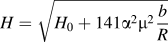 $H = \sqrt {{H_0} + 141{\alpha ^2}{\mu ^2}{b \over R}}$ in terms of the spherical indenter radius R and original indentation hardness H 0
 $\left( {{H_0} = 2.8{\sigma _{\rm{ref}}f\left( {{\varepsilon ^{\rm{p}}} = {a \over {5R}}} \right)} \right)$. Huang et al.Reference Huang, Zhang, Hwang, Nix, Pharr and Feng8 established an analytical model for nanoindentation hardness based on the maximum allowable geometrically necessary dislocation density. Recently, Cao et al.Reference Cao, Xue, Chen and Raabe15 studied the sharp indentation in soft metals and found a simple relation between the nominal hardness, H n, and the flow stress, σr, i.e., H n = 4.4σr.
Based on the previous research, this study focuses on the hardness with different combinations of material properties with considering size effect. To establish an integrated relationship for solving the forward problem, a model has been derived from the simulation results to set up the correlation between hardness and material elastic–plastic properties (E, σy, n). For the established model, it is not only a combination of material properties and size effect relating to hardness, but also a bridge between maximum load and loading curvature, and material properties. Furthermore, the characteristic length h ∗ in Nix/Gao model is rewritten and discussed with material properties accordingly.
II. THEORY AND EXPERIMENT
A. Theory of indentation experiments
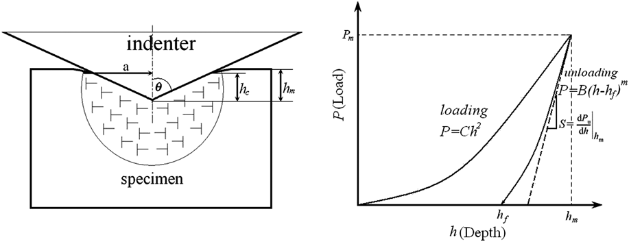
In the indentation field, Oliver and PharrReference Oliver and Pharr3,Reference Oliver and Pharr4 showed their methods based on the Berkovich indenters. The law relating to the applied load, P, to the penetration depth, h, follows Kick's law (see Fig. 1):
 $$P = C{h^2}\quad,$$
where C is the loading curvature which depends on elastic and plastic material properties, as well as indenter geometry.Reference Gouldstone, Chollacoop, Dao, Li, Minor and Shen1 Similarly, the unloading curve follows a simple power–law relation determined by a least square fitting procedure:
 $$P = B \times {(h - {h_{\rm{f}}})^m}\quad,$$
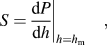
in which B and m are fitting parameters and h f is the residual depth after complete unloading. The elastic contact stiffness, S, is given by the first derivative at the peak load of unloading curve:
 $$S = {\left. {{{{\rm{d}}P} \over {{\rm{d}}h}}} \right|_{h = {h_{\rm{m}}}}}\quad,$$
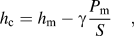
where h m is the maximum penetration depth. The depth, along which contact is made between the indenter and the specimen, can be estimated and given by
 $${h_{\rm{c}}} = {h_{\rm{m}}} - \gamma {{{P_{\rm{m}}}} \over S}\quad,$$
where P m is the maximum load at the onset of unloading, and γ is a tip-dependent geometry factor, which is equal to 0.72 for a conical indenter, 0.75 for a Berkovich indenter, and 1 for a flat cylindrical indenter.Reference Gouldstone, Chollacoop, Dao, Li, Minor and Shen1,Reference Oliver and Pharr4 From the knowledge of h c and the indenter parameter k = πtan2θ, the developed contact area, A, can be given byReference Ma and Clarke21
 $$A = kh_{\rm{c}}^2 = \pi {\tan ^2}\theta h_{\rm{c}}^2\quad.$$
Sketch of indentation process and P–h curve.

Consequently, the hardness of testing material can be determined as
 $$H = {{{P_{\rm{m}}}} \over A}\quad.$$
B. Simulation process
For simulation, a two-dimensional axisymmetric finite element model is constructed to simulate the indentation process by ABAQUS/Standard.Reference Hibbit22 The indenter is assumed to an equivalent cone and the tip apex angle θ is chosen as 70.3° for Berkovich indenter.Reference Gouldstone, Chollacoop, Dao, Li, Minor and Shen1,Reference Dao, Chollacoop, Van Vliet, Venkatesh and Suresh2,Reference Cheng and Cheng5 As shown in Fig. 2, it is the designed model which contains 2500 elements using quadrilateral elements. According to the study by Mata and Alcala,Reference Mata and Alcala23 the friction has great influence on considerable piling-up effects and little influence on moderate pileup or sinking-in. In this paper, the piling-up and sinking-in effects are not mentioned, so the friction between the indenter and the solid is set as frictionless tangential.Reference Mata and Alcala23 The input material constitutive model is written asReference Gouldstone, Chollacoop, Dao, Li, Minor and Shen1,Reference Dao, Chollacoop, Van Vliet, Venkatesh and Suresh2
 $$\sigma = \left\{ {\matrix{ {E\varepsilon } \cr {\sigma _{\rm{y}} \left( {1 + {E \over {\sigma _{\rm{y}} }}\varepsilon _{\rm{p}} } \right)^n } \cr } } \right.\quad \matrix{ {{\rm{for}}\quad \sigma \le \sigma _{\rm{y}} } \cr {{\rm{for}}\quad \sigma \ge \sigma _{\rm{y}} } \cr }\quad .$$
The simulation model.
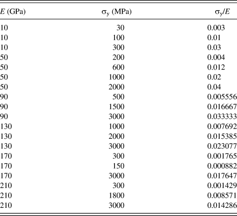
The material properties are selected as used in the study by Dao et al.Reference Dao, Chollacoop, Van Vliet, Venkatesh and Suresh2 shown in Table I with different strain hardening exponent, n = 0.1, 0.2, 0.3, 0.4, 0.5.Reference Dieter24 Also, different indentation depths are chosen in the range of 1, 1.5, 2, 2.5, 3 μm. The Poisson’s ratio of all the materials is fixed as ν = 0.33.
The material properties as used in the study of Dao et al.Reference Dao, Chollacoop, Van Vliet, Venkatesh and Suresh2
III. RESULTS AND DISCUSSION
A. Simulation results
After simulation, the relationship between the calculated hardness, the ratio of σy/E, and indentation depth h for different material properties is depicted in Fig. 3(a). Obviously, it can be seen that as the indentation depth decreased and the strain hardening exponent increased, the ratios of H/σy increase accordingly. In terms of Fig. 3(b), the ratios of h c/h m increase with the indentation depth and decreasing strain hardening exponent, however, it is not distinct with the increasing σy/E. Besides, P m/σy increases with the increasing indentation depth and strain hardening exponent, see Fig. 3(c). According to Eq. (1), the fitting loading curvature C is also plotted as shown in Fig. 3(d). With the increasing indentation depth h, C is decreasing a little, and it increases with the increasing strain hardening exponent. Still, no clear trend with σy/E can be found.
The relation between (a) H/σy; (b) hc/hm; (c) Pm/σy; (d) loading curvature C; versus σy/E at different indentation depth.
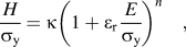
In a certain indentation depth, the H/σy is a function of σy/E and strain hardening exponent. To find a clear relation between hardness and material properties, a model is adopted as
 $${H \over {{\sigma _{\rm{y}}}}} = \kappa {\left( {1 + {\varepsilon _{\rm{r}}}{E \over {{\sigma _{\rm{y}}}}}} \right)^n}\quad,$$
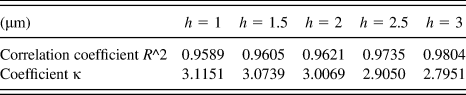
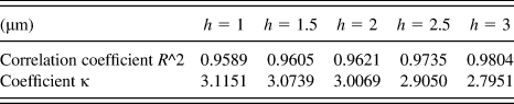
where κ is the coefficient and εr is the representative strain. Although the representative strain defined by Dao et al. only works for a limited property range,Reference Cao and Huber25 the representative strain in this paper was chosen as 0.033 as given in Ref. Reference Dao, Chollacoop, Van Vliet, Venkatesh and Suresh2, due to the material properties selected as shown in Table I. By using Eq. (8), the fitting results of κ are shown in Table II. It can be seen that as the indentation depth increases, the coefficient decreases. From this result, it is hard for us to get a uniform model to characterize the material properties. So, the indentation depth (size effect) should also be considered simultaneously at this level.
The fitting results by using Eq. (8).
B. The relation between microhardness and material properties
According to Cheng and Cheng,Reference Cheng and Cheng19 the relationship between microhardness, material properties (E, n, σy, ν), and simulation parameters (indenter angle θ) at certain indentation depth h, where the friction effect was not considered, can be written as
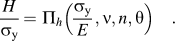 $${H \over {{\sigma _{\rm{y}}}}} = {\Pi _h}\left( {{{{\sigma _{\rm{y}}}} \over E},\nu ,n,\theta } \right)\quad.$$
If the indentation depth size effect is considered, Eq. (9) can be rewritten as
 $$H = H({\kappa _0},E,n,{\sigma _{\rm{y}}},\nu ,h,{h^ * })\quad.$$
In general, the material hardness is related to the material flow stress σflow asReference Gouldstone, Chollacoop, Dao, Li, Minor and Shen1,Reference Dao, Chollacoop, Van Vliet, Venkatesh and Suresh2,Reference Cheng and Cheng5,Reference Cheng and Cheng19
 $${H_0} = {\kappa _0}{\sigma _{{\rm{flow}}}}\quad,$$
where H 0 is the hardness of the material at macroscale, corresponding to the measured hardness at the greatest depth tested,Reference Swadener, George and Pharr26 and σflow is the uniaxial tensile flow stressReference Huang, Zhang, Hwang, Nix, Pharr and Feng8 or representative stress. κ0 is a constraint factor depending on indenter angle and material properties, which increases with E/σy (or 1/εy) and approaches a constant (∼3) when E/tanθ(1−ν2)σy > 20.Reference Chen and Vlassak27,Reference Johnson28 The constraint factor κ0 is 2.75 referring to the study by Cheng and Cheng.Reference Cheng and Cheng18
According to the study by Huang et al.,Reference Huang, Zhang, Hwang, Nix, Pharr and Feng8 the flow stress is determined from the uniaxial tension stress–strain curve, which is related to the plastic strain εp as
 $${\sigma _{{\rm{flow}}}} = {\sigma _{{\rm{ref}}}}f({\varepsilon ^{\rm{p}}})\quad,$$
where σref is a reference stress and f(εp) is a nondimensional function, which can be written in a different form according to the material properties adopted.Reference Cheng and Cheng5,Reference Huang, Zhang, Hwang, Nix, Pharr and Feng8,Reference Wei and Hutchinson17
Combining Eqs. (11) and (12), the relationship between hardness and flow stress can be rewritten as
 $${H_0} = {\kappa _0}{\sigma _{{\rm{ref}}}}f({\varepsilon ^{\rm{p}}})\quad.$$
Here, the reference stress is taken as σref = σy, and the function of plastic strain from Huang et al.Reference Huang, Zhang, Hwang, Nix, Pharr and Feng8 is
 $$f({\varepsilon ^{\rm{p}}}) = {\left( {1 + {E \over {{\sigma _{\rm{y}}}}}{\varepsilon ^{\rm{p}}}} \right)^n} = {\left( {1 + {{{\varepsilon ^{\rm{p}}}} \over {{\varepsilon ^{\rm{y}}}}}} \right)^n}\quad.$$
Using Eq. (14) and σref = σy in Eq. (13), it can be rewritten as
 $${H_0} = {\kappa _0}{\sigma _{{\rm{flow}}}} = {\kappa _0}{\sigma _{{\rm{ref}}}}f({\varepsilon ^{\rm{p}}}) = {\kappa _0}{\sigma _{\rm{y}}}{\left( {1 + {E \over {{\sigma _{\rm{y}}}}}{\varepsilon ^{\rm{p}}}} \right)^n}\quad.$$
If εp is chosen as a representative strain εr, the relationship can be obtained, which agrees with Eq. (8):
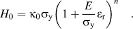 $${H_0} = {\kappa _0}{\sigma _{\rm{y}}}{\left( {1 + {E \over {{\sigma _{\rm{y}}}}}{\varepsilon _{\rm{r}}}} \right)^n}\quad.$$
From the previous research studies on size effect,Reference Nix and Gao7,Reference Huang, Zhang, Hwang, Nix, Pharr and Feng8,Reference Durst, Backes and Göken13 the material hardness at microscale is
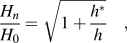 $${{{H_n}} \over {{H_0}}} = \sqrt {1 + {{{h^*}} \over h}}\quad ,$$
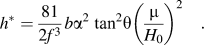 $${h^*} = {{81} \over {2{f^3}}}b{\alpha ^2}\;{\tan ^2}\theta {\left( {{\mu \over {{H_0}}}} \right)^2}\quad.$$
In the above equations, H 0 is the macroscopic hardness, relating to the density of statistically stored dislocations (SSDs) according to Nix/Gao model and h ∗ is a characteristic length for the material.Reference Nix and Gao7 If the hardness H 0 in Eqs. (16) and (17a) is the same, and using Eq. (16) in Eq. (17a), one can find
 $$H = H({\kappa _0},E,n,{\sigma _{\rm{y}}},\nu ,h,{h^ * }) = {H_0}\sqrt {1 + {{{h^*}} \over h}} = {\kappa _0}{\sigma _{\rm{r}}}\sqrt {1 + {{{h^*}} \over h}} = {\kappa _0}{\sigma _{\rm{y}}}{\left( {1 + {E \over {{\sigma _{\rm{y}}}}}{\varepsilon _{\rm{r}}}} \right)^n}\sqrt {1 + {{{h^*}} \over h}}\quad .$$
It is the relationship between hardness and material properties with considering size effect at a certain Poisson’s ratio. In the proposed model as in Eq. (18), h ∗ relates to the material properties, definitely not a constant for all materials. It is related to the intrinsic characteristic length associating with size effect, as shown in Eq. (17b). If shear modulus,  $\mu = {E \over {2(1 + \nu )}}$ and macroscopic hardness
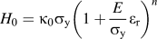 ${H_0} = {\kappa _0}{\sigma _{\rm{y}}}{\left( {1 + {E \over {{\sigma _{\rm{y}}}}}{\varepsilon _{\rm{r}}}} \right)^n}$ with representative strain εr = 0.033 as in the study by Dao et al.Reference Dao, Chollacoop, Van Vliet, Venkatesh and Suresh2 are substituted in Eq. (18), the model is determined as
$$H = {\kappa _0}{\sigma _{\rm{y}}}{\left( {1 + {E \over {{\sigma _{\rm{y}}}}}{\varepsilon _{\rm{r}}}} \right)^n}\sqrt {1 + {{81} \over {2{f^3}h}}b{\alpha ^2}\;{{\tan }^2}\theta {{\left( {{\mu \over {{H_0}}}} \right)}^2}} = {\kappa _0}{\sigma _{\rm{y}}}{\left( {1 + {E \over {{\sigma _{\rm{y}}}}}{\varepsilon _{\rm{r}}}} \right)^n}\sqrt {1 + {{81} \over {2{f^3}h}}b{\alpha ^2}\;{{\tan }^2}\theta {{\left( {{E \over {2(1 + \nu ){\kappa _0}{\sigma _{\rm{y}}}{{\left( {1 + {E \over {{\sigma _{\rm{y}}}}}{\varepsilon _{\rm{r}}}} \right)}^n}}}} \right)}^2}\quad}.$$ For a Berkovich indenter, θ = 70.3°, Burgers vector b is at quality of 10−4 μm, and empirical coefficient is α = 0.1–0.5. So, the part of 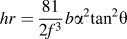 $hr = {{81} \over {2{f^3}}}b{\alpha ^2}{\tan ^2}\theta$ should be at the order of magnitude of 10−4–10−2. From the proposed model, a better fitting result is obtained with the constraint factor as κ0 = 2.90016, and hr = 0.000613247, which meets the requirement of magnitude order, with correlation coefficient (R): 0.9839. The proposed model reflects a good relationship between material hardness and their properties.
By the process of Nix and Gao, H 0 can be obtained by the linear fitting H 2 versus h −1 by 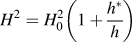 ${H^2} = H_0^2\left( {1 + {{{h^*}} \over h}} \right)$.Reference Nix and Gao7 With the simulation results, the relationship between the fitting H 0 and predicted H 0 is plotted in Fig. 4, where predicted hardness
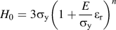 ${H_0} = 3{\sigma _{\rm{y}}}{\left( {1 + {E \over {{\sigma _{\rm{y}}}}}{\varepsilon _{\rm{r}}}} \right)^n}$, in which the constraint factor is set as 3.Reference Cheng and Cheng5,Reference Tabor20 We can find that the predicted H 0 is a bit greater than experimental results. The reason can be explained by the previous fitting result κ0 = 2.90016, which is less than the traditional one used.Reference Cheng and Cheng5,Reference Tabor20
The relationship between the experiment H 0 and predicted H 0.
In microscale, the hardness of solids is determined by many factors, such as material elastic–plastic properties (E, σy, n), indenter geometry (half apex angle, indenter shape), friction factor, etc.Reference Cheng and Cheng5,Reference Cheng and Cheng18,Reference Johnson28 To find a proper and precise relation between hardness and material properties, the forward problem has been focused on since long.Reference Cheng and Cheng5,Reference Cheng and Cheng18,Reference Tabor20,Reference Johnson28 Tabor proposed that the hardness is 3 times of the flow stress at 8% representative strain.Reference Gouldstone, Chollacoop, Dao, Li, Minor and Shen1 The result of Johnson for a large indent in an elastic–perfectly plastic solid is  $H = {2 \over 3}{\sigma _{\rm{y}}}(1 + \ln (\tan \beta /3{\varepsilon _{\rm{y}}}))$, which is in agreement with the limit for large indents for the solid with low strain hardening.Reference Wei and Hutchinson17,Reference Johnson28 Following Tabor's model, Cheng and Cheng set up a model between hardness and representative stress (the yield stress at 10% of strain) with a different yield strain, since with great representative strain, the effect of strain hardening exponent vanished.Reference Cheng and Cheng19 As used in the concept, the material hardness is independent to indentation depth.Reference Cheng and Cheng5 This previous model was not considered size effect at microscale, which cannot obtain better results in this study. In regard to the model of Eq. (18) with size effect, the part of
 $\sqrt {1 + {{{h^*}} \over h}}$ is combined with material properties. When the indentation depth is large enough, the part of
 $\sqrt {1 + {{{h^*}} \over h}}$ will be close to 1, and then the hardness will not relate to size effect and just depends on material properties. Besides, according to Cao et al.,Reference Cao, Xue, Chen and Raabe15 he defined a new hardness as H 0n, which is the nominal hardness at the macroscaleReference Cao, Xue, Chen and Raabe15 or is the hardness in the limit of infinite depth.Reference Nix and Gao7 It was H n = 4.4σr, in which the constraint factor κ0 was set as 4.4, different from the general result κ0 = 3.Reference Ogasawara, Chiba and Chen14,Reference Chen and Vlassak27 According to the proposed model,
 $H = {H_0}\sqrt {1 + {{{h^*}} \over h}} = {\kappa _0}{\sigma _{\rm{r}}}\sqrt {1 + {{{h^*}} \over h}}\,$, at an infinite size or indentation depth h 0n, the material hardness is given as
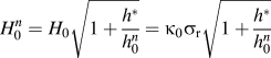 $H_0^n = {H_0}\sqrt {1 + {{{h^*}} \over {h_0^n}}} = {\kappa _0}{\sigma _{\rm{r}}}\sqrt {1 + {{{h^*}} \over {h_0^n}}}\,$. Combining the part of
 ${\kappa _0}\sqrt {1 + {{{h^*}} \over {h_0^n}}}\,$, it is greater than 3 for the nominal hardness of the material at an infinite size, or at the limitation of size effect, which is similar to the results of Cao et al.Reference Cao, Xue, Chen and Raabe15 For h 0n, it may be related to the limited depth of size effect, which is needed for further investigation.
Accordingly, by using Eqs. (1) and (6) the maximum load is determined as
 $${P_{\rm{m}}} = {P_{\rm{m}}}({\kappa _0},E,n,{\sigma _{\rm{y}}},\nu ,h,{h^ * }) = HA = kh_{\rm{c}}^2H = kh_{\rm{c}}^2{\kappa _0}{\sigma _{\rm{y}}}{\left( {1 + {\varepsilon _{\rm{r}}}{E \over {{\sigma _{\rm{y}}}}}} \right)^n}\sqrt {1 + {{{h^*}} \over h}}\quad .$$
As given in Eq. (6), the hardness H is the ratio between maximum load P m and contact area A: 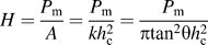 $H = {{{P_{\rm{m}}}} \over A} = {{{P_{\rm{m}}}} \over {kh_{\rm{c}}^2}} = {{{P_{\rm{m}}}} \over {\pi {{\tan }^2}\theta h_{\rm{c}}^2}}$.
C. The relationship between loading curvature and material properties
Similarly, loading curvature C, which depends on elastic and plastic material properties, as well as indenter geometry,Reference Gouldstone, Chollacoop, Dao, Li, Minor and Shen1 is the ratio of load and indenter depth h by Eq. (1). During indentation process, C is a constant, which can be obtained from the fitting process as shown in Fig. 5. Also, it can be determined at peak depth h m as 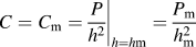 $C = {C_{\rm{m}}} = {\left. {{P \over {{h^2}}}} \right|_{h = h{\rm{m}}}} = {{{P_{\rm{m}}}} \over {h_{\rm{m}}^2}}$, which is similar to the definition as hardness H. One relates to the contact depth h c, and the other associates to the maximum depth h m. From Eq. (6), it can be found that C mh m2 = Hkh c2. So, loading curvature C can be determined as
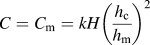 $C = {C_{\rm{m}}} = kH{\left( {{{{h_{\rm{c}}}} \over {{h_{\rm{m}}}}}} \right)^2}$. From the obtained results as shown in Fig. 3(d), the relationship between C and
 $H{\left( {{{{h_{\rm{c}}}} \over {{h_{\rm{m}}}}}} \right)^2}$ is fitted, a good result for coefficient k is obtained as 24.399–24.673, which is close to the value of k = πtan2θ = 24.56, with correlation coefficient (R): 0.9997 (see Fig. 6).
Examples of fitting loading curvature C with n = 0.3 and h = 1 (red lines are the fitting lines and scattered symbols are the original data).
The relation between loading curvature C and H(h c/h m)2.
Accordingly, combining Eqs. (18), (20), and (1), the loading curvature C can be rewritten as
 $$C = kH{\left( {{{{h_{\rm{c}}}} \over {{h_{\rm{m}}}}}} \right)^2} = k{\kappa _0}{\sigma _{\rm{r}}}{\left( {{{{h_{\rm{c}}}} \over {{h_{\rm{m}}}}}} \right)^2}\sqrt {1 + {{{h^*}} \over {{h_{\rm{m}}}}}} = k{\kappa _0}{\sigma _{\rm{y}}}{\left( {1 + {\varepsilon _{\rm{r}}}{E \over {{\sigma _{\rm{y}}}}}} \right)^n}{\left( {{{{h_{\rm{c}}}} \over {{h_{\rm{m}}}}}} \right)^2}\sqrt {1 + {{{h^*}} \over {{h_{\rm{m}}}}}}\quad ,$$
in which C depends on elastic and plastic material properties, as well as indenter geometry.Reference Gouldstone, Chollacoop, Dao, Li, Minor and Shen1 From Eq. (21), loading curvature C is related to the material properties with  ${\kappa _0}{\sigma _{\rm{r}}}\sqrt {1 + {{{h^*}} \over {{h_{\rm{m}}}}}}$, i.e., the macronominal hardness, H 0, indenter geometry k = πtan2θ, and certain ratio between contact depth and maximum depth
 $\left( {{{{h_{\rm{c}}}} \over {{h_{\rm{m}}}}}} \right)$, which vary slightly with increasing indentation depth.
D. Characteristic length h ∗
For size effect, the hardness relates to the dislocation in the material during deformation as GND density (ρG) which responds to the ‘additional’ hardness, and the original SSDs density (ρS) and the size effect of the material can be rewritten as
 $${{{H_{\rm{n}}}} \over {{H_0}}} = \sqrt {1 + {{{h^*}} \over h}} = \sqrt {1 + {{{\rho _{\rm{G}}}} \over {{\rho _{\rm{S}}}}}}\quad ,$$
 $${h^*} = {{{\rho _{\rm{G}}}} \over {{\rho _{\rm{S}}}}}h\quad.$$
in which h ∗ is not a constant for a given material and indenter geometry. Rather it depends on the SSD density through H 0.Reference Nix and Gao7 And GND density (ρG) and SSD density (ρS) are
 $${\rho _{\rm{G}}} = \bar r{{{\eta ^p}} \over b} = {3 \over {2{f^3}\;{{\tan }^2}\theta bh}}\quad,$$
 $${\rho _{\rm{S}}} = {[{\sigma _{{\rm{ref}}}}f({\varepsilon ^{\rm{p}}})/(M\mu \alpha b)]^2}\quad,$$
in which a coefficient f is added into GND density [ρG as Eq. (23b)], when the profile of indenter shape is not considered,Reference Durst, Backes and Göken13,Reference Swadener, George and Pharr26 and M is the Taylor factor which acts as an isotropic interpretation of the crystalline anisotropy at the continuum level, M = 3 for FCC metals as well as for BCC metals on {1 1 0} slip planes. The relation between GND density (ρG) and SSD density (ρS) is
 $${{{\rho _{\rm{G}}}} \over {{\rho _{\rm{S}}}}} = {{{3 \over {2{f^3}{{\tan }^2}\theta bh}}} \over {{{[{\sigma _{{\rm{ref}}}}f({\varepsilon ^{\rm{p}}})/(M\mu \alpha b)]}^2}}} = {{3{{(M\mu \alpha )}^2}b} \over {2{f^3}{{\tan }^2}\theta h{{[{\sigma _{{\rm{ref}}}}f({\varepsilon ^{\rm{p}}})]}^2}}}\quad.$$
And h ∗ can be rewritten as
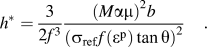 $${h^ * } = {3 \over {2{f^3}}}{{{{(M\alpha \mu )}^2}b} \over {{{({\sigma _{{\rm{ref}}}}f({\varepsilon ^{\rm{p}}})\tan \theta )}^2}}}\quad.$$
In Nix and Gao,Reference Nix and Gao7 the hardness also was determined as
 $${H_0} = {\kappa _0}M\alpha \mu b\sqrt {{\rho _{\rm{S}}}}\quad .$$
In Nix/Gao model, the SSD density (ρS) was  ${\rho _{\rm{s}}} \approx {1 \over {L_{\rm{s}}^2}}$, where L s is the mean spacing between SSDs.Reference Nix and Gao7 However, for the case of materials strengthened by dispersoids or precipitations, the flow stress in the absence of gradients might be expressed in terms of the mean spacing between particles, L p,
 ${\rho _{\rm{s}}} \approx {1 \over {{{(\alpha {L_{\rm{p}}})}^2}}}$ according toReference Nix and Gao7
 $${\rho _{\rm{s}}} \approx {1 \over {L_{\rm{s}}^2}}\quad,$$
 $${\rho _{\rm{s}}} \approx {1 \over {{{(\alpha {L_{\rm{p}}})}^2}}}\quad.$$
Referring to Eqs. (16) and (26), the SSD density (ρS) can be rewritten as
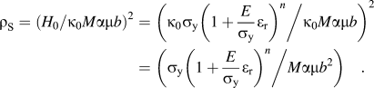 $${\rho _{\rm{S}}} = {({H_0}/{\kappa _0}M\alpha \mu b)^2} = {\left( {{{{\kappa _0}{\sigma _{\rm{y}}}{{\left( {1 + {E \over {{\sigma _{\rm{y}}}}}{\varepsilon _{\rm{r}}}} \right)}^n}} \mathord{\left/ {\vphantom {{{\kappa _0}{\sigma _{\rm{y}}}{{\left( {1 + {E \over {{\sigma _{\rm{y}}}}}{\varepsilon _{\rm{r}}}} \right)}^n}} {{\kappa _0}M\alpha \mu b}}} \right. \kern-\nulldelimiterspace} {{\kappa _0}M\alpha \mu b}}} \right)^2} = \left( {{{{\sigma _{\rm{y}}}{{\left( {1 + {E \over {{\sigma _{\rm{y}}}}}{\varepsilon _{\rm{r}}}} \right)}^n}} \mathord{\left/ {\vphantom {{{\sigma _{\rm{y}}}{{\left( {1 + {E \over {{\sigma _{\rm{y}}}}}{\varepsilon _{\rm{r}}}} \right)}^n}} {M\alpha \mu {b^2}}}} \right. \kern-\nulldelimiterspace} {M\alpha \mu {b^2}}}} \right)\quad.$$
According to Eq. (27c), SSD density (ρS) is related to the material properties, i.e., the macronominal hardness, H 0. When the material is selected, the SSD density mainly depends on the deformation degree in the material. With the increasing plastic strain, the SSD density (ρS) increases accordingly. Additionally, the loading curvature is related to dislocation density as 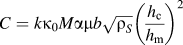 $C = k{\kappa _0}M\alpha \mu b\sqrt {{\rho _S}} {\left( {{{{h_{\rm{c}}}} \over {{h_{\rm{m}}}}}} \right)^2}$.
Moreover, if GND density (ρG) is taken as given in Ref. Reference Durst, Backes and Göken13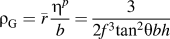 ${\rho _{\rm{G}}} = \bar r{{{\eta ^p}} \over b} = {3 \over {2{f^3}{{\tan }^2}\theta bh}}$, in which a coefficient f was used for the plastic deformation scope under indenter tip.Reference Durst, Backes and Göken13 Accordingly, the characteristic length h ∗ is determined as
 $${h^*} = {{{3 \over {2{f^3}{{\tan }^2}\theta bh}}} \over {{\rho _{\rm{S}}}}}h = {3 \over {2b{f^3}{\rho _{\rm{S}}}{{\tan }^2}\theta }}\quad.$$
Substituting SSD density (ρS) in Eq. (28), h ∗ can be rewritten as
 $$h^* = \left\{ {\matrix{ {{{3L^2 _{\rm{S}} } \over {2bf^3 \tan ^2 \theta }}} \cr {{{3\alpha ^2 L^2 _{\rm{P}} } \over {2bf^3 \tan ^2 \theta }}} \cr } } \right.\quad \matrix{ {{\rm{for}}\;{\rm{pure}}\;{\rm{metal}}} \cr {{\rm{for}}\;{\rm{strengthened}}\;{\rm{materials}}} \cr }\quad ,$$
or
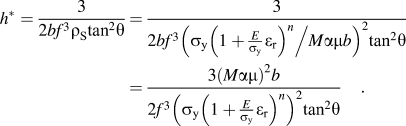 $${h^*} = {3 \over {2b{f^3}{\rho _{\rm{S}}}{{\tan }^2}\theta }} = {3 \over {2b{f^3}{{\left( {{{{\sigma _{\rm{y}}}{{\left( {1 + {E \over {{\sigma _{\rm{y}}}}}{\varepsilon _{\rm{r}}}} \right)}^n}} \mathord{\left/ {\vphantom {{{\sigma _{\rm{y}}}{{\left( {1 + {E \over {{\sigma _{\rm{y}}}}}{\varepsilon _{\rm{r}}}} \right)}^n}} {M\alpha \mu b}}} \right. \kern-\nulldelimiterspace} {M\alpha \mu b}}} \right)}^2}{{\tan }^2}\theta }} = {{3{{(M\alpha \mu )}^2}b} \over {2{f^3}{{\left( {{\sigma _{\rm{y}}}{{\left( {1 + {E \over {{\sigma _{\rm{y}}}}}{\varepsilon _{\rm{r}}}} \right)}^n}} \right)}^2}{{\tan }^2}\theta }}\quad.$$
The characteristic length h ∗ only depends on the material properties, especially the average distance between dislocations or dispersoids or precipitations. With the increasing SSD density or dispersoids or precipitations, the distance between them is reduced accordingly. This effect strengthens the material with small characteristic length h ∗. Furthermore, the value of characteristic length h ∗ is a measurement for size effect. When the ratio of h ∗/h is small enough at great indentation depth, the material hardness will become constant, while it is sensitive to indentation depth when the ratio of h ∗/h is a non-missing part.
IV. CONCLUSION
By using a two-dimensional axisymmetric finite element model, the indentation hardness has been studied with different combinations of material properties with considering size effect. Based on the previous research on size effect, a model of correlation between several indentation experiment parameters (hardness H, maximum load P m, and loading curvature C) and material properties (E, σy, and n) has been derived. From the simulation results, a better fitting result is obtained from the model with size effect. Furthermore, the characteristic length h ∗ in Nix/Gao model has been rewritten and discussed accordingly.
ACKNOWLEDGMENTS
The authors are very grateful for the support received from the Aeronautical Science Foundation of China under Grant No. 2011ZE53059 and National Natural Science Foundation of China (51275414).