I. INTRODUCTION
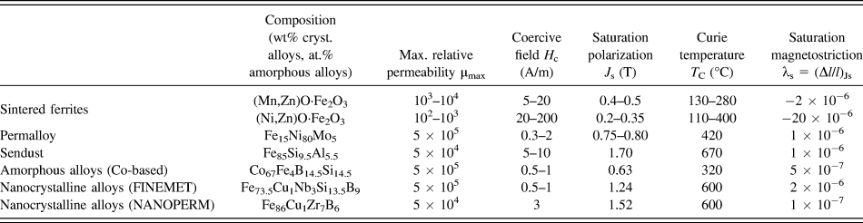
The soft magnetic materials nowadays available to industry are required to cover a tremendous array of applications, from the classical use as cores of transformers, generators, and motors, to the great variety of inductive components used in power electronics, sensing, automotive, household, recording, and telecommunication technologies. Remarkably, all these functions are covered with a handful of compositions, providing the best compromise among a number of requirements, of which the excellent soft magnetic behavior is not always the most important one. A vast and expanding applicative area for soft magnetic cores concerns a multitude of devices for electronics, which call for soft magnetic materials endowed with high permeability and low losses over a broad range of frequencies, from DC to several MHz. Relevant examples of applications are found in the switch-mode power supplies (SMPS), converters, inverters, radiofrequency interference filters, and magnetic amplifiers, where the core losses and the ensuing rise of temperature are main issues. Soft ferrites have traditionally dominated this field of applications. They are mixed oxides, having the general composition MO·Fe2O3, where M is a divalent metal ion such as Fe2+, Mn2+, Ni2+, Zn2+, and Mg2+. The Mn–Zn and Ni–Zn ferrite cores, obtained by sintering the oxide powders, are the standard industrial products, with the Ni–Zn types covering a broader frequency range, typically up to some 10 MHz versus a typical 1 MHz limit of Mn–Zn ferrites, at the cost of reduced permeability.Reference Snelling1 The key to the soft magnetic properties of ferrites is the so-called mechanism of “anisotropy compensation”,Reference Pascard2 where the negative magnetocrystalline anisotropy of the Fe3+ ions is compensated by the positive anisotropy of divalent cations, like Fe2+ or Co2+, introduced on purpose. With suitable concentration of these ions, the resultant magnetocrystalline anisotropy constant will cross the zero value at a convenient temperature (typically, between room temperature and 100 °C). Full anisotropy compensation is, for example, obtained at ∼25 °C with the composition Mn0.53Zn0.40Fe0.072+Fe23+O4.
A vanishing magnetic anisotropy opens the way to soft and extra-soft magnetic properties because the magnetization process, be it accomplished by domain wall (dw) displacements or rotation of the magnetic moments, is the easier the lower is the anisotropy energy (i.e., the anisotropy constant K). A simplified approach to the coercive field H c and the initial permeabilities by dw motion  $\mu _{\rm{i}}^{{\rm{dw}}}$ and rotations
 $\mu _{\rm{i}}^{{\rm{rot}}}$ provides
 $${H_{\rm{c}}} \propto {{{K^{1/2}}} \over {{J_{\rm{s}}}\left\langle s \right\rangle }},\quad \mu _{\rm{i}}^{{\rm{dw}}} \propto {{J_{\rm{s}}^2 \cdot \left\langle s \right\rangle } \over {{K^{1{\rm{/}}2}}}}\quad \mu _{\rm{i}}^{{\rm{rot}}} \propto {{J_{\rm{s}}^2} \over K}\quad ,$$
in a material of saturation polarization J s and average grain size 〈s〉.Reference Rossignol and du Trémolet de Lacheisserie3,Reference Fiorillo, Appino, Pasquale, Bertotti and Mayergoyz4
Permalloy and Sendust are trade names of alloys having compositions leading to simultaneous near zero magnetocrystalline anisotropy K and magnetostriction constant λs. In this way, also the anisotropy induced by local or applied stress σ, K σ = (3/2) λsσ, is minimized. Permalloy has typical composition Fe15Ni80Mo5 and attains vanishing magnetocrystalline anisotropy by compensation of the positive K of Fe with the negative K of Ni. Sendust is the ternary alloy Fe85Si9.5Al5.5, which is obtained in powder form and typically shaped as consolidated cores for magnetic heads. Because of their vanishing intrinsic anisotropy, Permalloy tapes are sensitive to magnetic field annealing and the correspondingly induced anisotropy. Consequently, they can display a range of hysteresis loop shapes, besides excellent response in broadband applications, but, like the Sendust alloy, they generally cover niche markets. In many such applications, the nanocrystalline alloys have a competitive advantage with respect to permalloys, as they come at a fraction of cost, and, as shown in Table I, they are endowed with higher saturation polarization (thereby withstanding better any DC field bias), while displaying superior temperature stability and similar versatility and magnetic softness. Nanocrystalline ribbons represent a smart alternative to permalloys, as they can, in spite of their metallic features, display excellent soft magnetic behavior at very high frequencies, as required, for example, in inductors of high-power-density SMPS. Vanishing magnetocrystalline anisotropy is achieved in these alloys thanks to their nanogranular structure, obtained by homogeneous crystallization of a precursor amorphous alloy produced by rapid solidification.Reference Yoshizawa, Oguma and Yamauchi5,Reference Makino, Inoue and Masumoto6 Here the anisotropy fluctuates from grain to grain, on a much smaller scale than the exchange length L ex, which encompasses a large number of nanometer-sized crystals, exchange coupled via the amorphous residual phase. The magnetic moments in the grains are therefore constrained to alignment by the exchange interaction and cannot follow the random directions of the local easy axes. Consequently, the local magnetocrystalline anisotropy K 1 is averaged out to a residual anisotropy K 0 across the N structural units of average size δ within the volume L ex3 = Nδ3 according to K 0 ≈ K 1/√N. For the classical case of a Finemet alloy Fe73.5Cu1Nb3B9Si13.5, having average nanograin size δ = 10 nm, one finds the faint residual anisotropy K 0 ∼ 2.5 J/m3.Reference Herzer7,Reference Herzer and Buschow8 Higher saturation magnetization than the one exhibited by Finemet (J s = 1.24 T) is obtained with the composition Fe86Cu1Zr3B9Si13.5 (Nanoperm, J s = 1.52 T), at the cost of increased coercivity and decreased permeability.Reference Makino, Inoue and Masumoto6 The operating temperature in both alloys is lower than 250 °C, because of the relatively low Curie temperature of the amorphous phase. Higher operating temperatures are obtained by the addition of Co, like in the nanocrystalline HITperm alloys, having composition Fe44Co44Zr7Cu1, where the high J s value is associated with improved mechanical properties.Reference Willard, Laughlin, McHenry, Thoma, Sickafus, Cross and Harris9 With partial substitution of Co with Ni, the relatively moderate soft magnetic properties of HITperm improve thanks to reduced magnetostriction. Nanocrystalline alloys of composition Fe77Ni8.25 Co2.75Zr7B4Cu1 show, for example, a coercive field of 12.5 A/m and a magnetostriction constant λs = 4.8 ⋅ 10−6.Reference Martone, Dong, Lan and Willard10 The concept of random anisotropy obviously applies to the amorphous alloys, where the ordered units are aggregates of few atoms.Reference Alben, Becker and Chi11 However, once the magnetocrystalline effects are made negligible, other sources of magnetic anisotropy emerge. This is the case of the magnetostrictive Fe-based amorphous alloys (like the popular Fe78B13Si9), where local anisotropies up to some 103 J/m3 can arise in the as-quenched ribbons because of the magnetoelastic coupling between frozen-in stresses and magnetization.Reference Kronmüller and Fernengel12,Reference Appino and Fiorillo13 Such stresses cannot be fully eliminated by annealing because the treatment temperature must be sufficiently low to avoid incipient inhomogeneous crystallization. It is to note that in the nanocrystalline alloys also the local magnetostrictive anisotropy is averaged out to a negligible value, bringing about stress insensitivity of the magnetic properties.Reference Herzer and Buschow8 Co-based amorphous alloys (like Co67Fe4B14.5Si14.5, Co71Fe4B15Si10, and Co66Fe5Cr4B15Si1) have vanishing magnetostriction (λs ∼ 10−8 to 10−7) and, obviously lacking any magnetocrystalline anisotropy, they can exhibit an extremely soft magnetic behavior, fully comparable to one of the nanocrystalline alloys (see Table I). The Co-based amorphous alloys display great versatility and sensitivity to magnetic annealing, besides excellent broadband soft magnetic response. They are not affected by the extreme brittleness of the nanocrystalline alloys, but their low saturation magnetization and the costs associated with the presence of Co limit their use to specialized applications. In these alloys, the anisotropy induced by field annealing is ascribed to atomic rearrangements of the local ordered units, whose symmetry is influenced by the direction of the magnetization,Reference Morita, Obi, Fujimori, Steeb and Warlimont14 while directional pair ordering of the Si atoms in the Fe–Si nanocrystals is invoked for the nanocrystalline alloys.Reference Herzer and Buschow8 High uniaxial transverse anisotropies, up to some kJ/m3, can be induced in amorphous and nanocrystalline ribbons by annealing under tensile stress,Reference Kraus, Závěta, Heczko, Duhaj, Vlasák and Schneider15,Reference Alves and Barrué16 an effect that is thought to descend from thermally activated anelastic creep and ensuing redistribution of the atomic bonds in the amorphous phase, which are frozen-in upon cooling and stress removal.Reference Suzuki, Haimovich and Egami17
Typical compositions and basic magnetic parameters of soft magnetic materials for broadband applications.
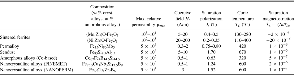
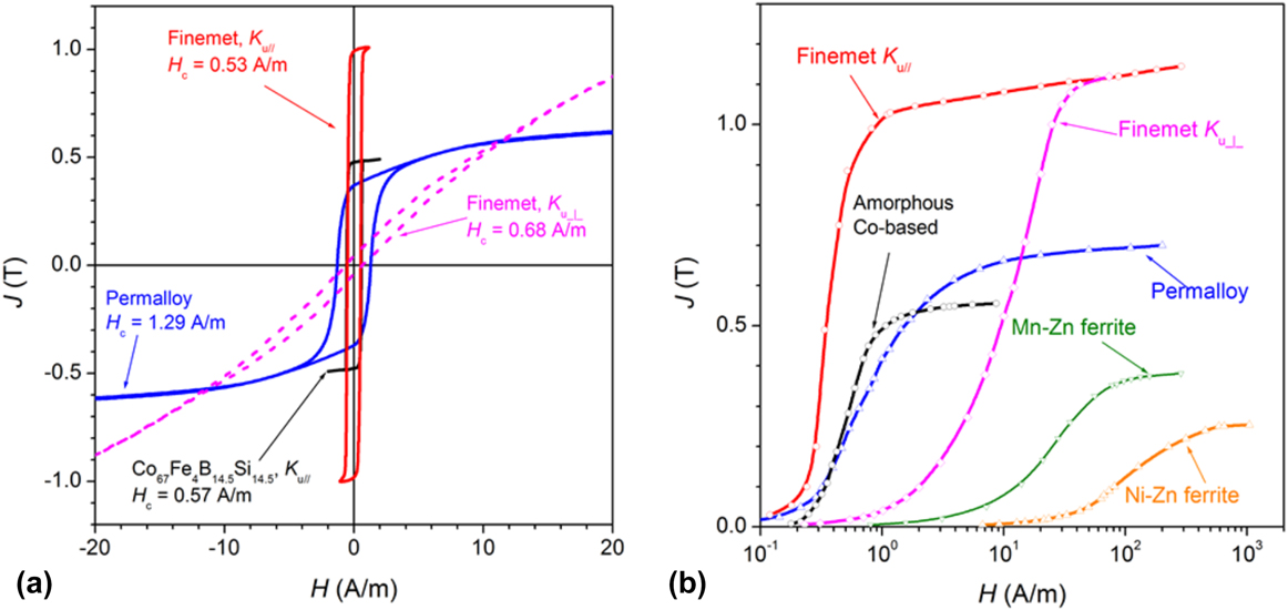
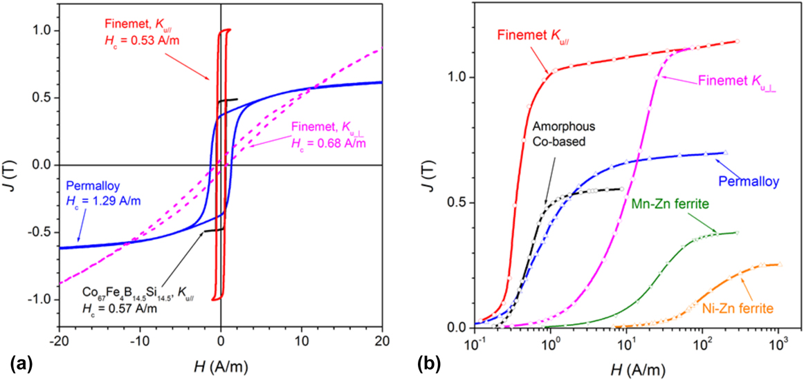
Figure 1 provides an overview of the quasi-static magnetic behavior of Permalloy tapes, Finemet and amorphous Co-based ribbons, and sintered Mn–Zn and Ni–Zn ring samples. An example of loop shearing in the Finemet ribbon by annealing under a saturating transverse field is provided. It is remarked how this can occur by inducing quite a low transverse anisotropy (K u⊥ ∼ 15 J/m3), a feature conducive to excellent frequency response, in terms of high permeability, high cutoff frequency, and low losses. The high transverse anisotropy arising upon stress annealing provides instead a very good alternative to cut cores for choke coils and linear inductors.Reference Fukunaga, Furukawa, Tanaka and Nakano18 Nanocrystalline samples come as thin (typically around 20 μm) ribbons and their resistivity is relatively high (ρ = 118 × 10−8 Ω m in Finemet). These properties are helpful in limiting the energy dissipation by eddy currents and in broadening the useful frequency band. They are shared by the Co-based amorphous alloys (see Table I), including the resistivity value (ρ = 141 × 10−8 Ω m in Co67Fe4B14.5Si14.5), but for the saturation magnetization. It is then verified that similar good loss and permeability behaviors deep into the MHz range are obtained in both alloysReference Herzer and Buschow8,Reference Magni, Bottauscio, Beatrice, Caprile, Ferrara and Fiorillo19,Reference Fiorillo, Bertotti, Appino, Pasquale and Peterca20 because of the strict similarities of their static and dynamic response to the induced anisotropy. But, properly annealed amorphous ribbons are not so brittle and allow for easier and more comprehensive magneto-optical analysis of the dw dynamics than nanocrystalline samples.Reference Magni, Bottauscio, Beatrice, Caprile, Ferrara and Fiorillo19
(a) Quasi-static major hysteresis loops of soft magnetic materials for broadband applications (Permalloy Fe15Ni80Mo5, amorphous alloy Co67Fe4B14.5Si14.5, nanocrystalline (Finemet) alloy Fe73.5Cu1Nb3B9Si13.5). All these materials are obtained as ribbons. Either longitudinal K u‖ or transverse K u⊥ anisotropy is induced by annealing under a saturating magnetic field. Quasi-linear J(H) curve with K u⊥ ∼ 15 J/m3 is shown for the Finemet alloy. (b) The normal magnetization curves of the same alloys are compared with those of the sintered Mn–Zn and Ni–Zn ferrites.
In recent times, interest has been devoted to conglomerates of either amorphous or nanocrystalline particles, obtained by a host of methods,Reference Otsuka, Wada, Maeta, Kadomura and Yagi21,Reference Mazaleyrat and Varga22 by which one can manufacture net-shaped parts through particle bonding or sintering, without need for further tooling. Three-dimensional fluxes can in this way be accommodated. Because of the distributed air-gaps, these materials exhibit low permeabilities, typically in the range 20–200, and the initial permeability can maintain a constant value up to the MHz range.Reference Shokrollahi and Janghorban23,Reference Füzer, Bednarčík, Kollár and Roth24
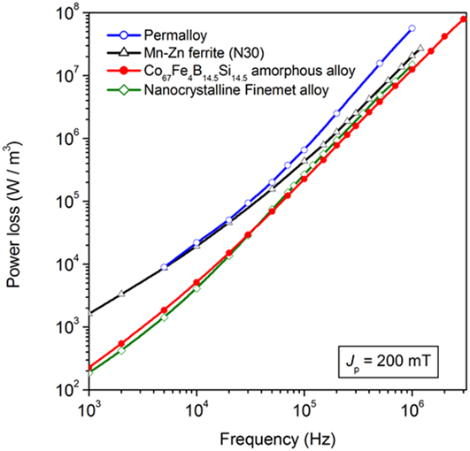
The very high resistivity of ferrites (typically 1–10 Ω m in Mn–Zn and some 105 Ω m in Ni–Zn) is equally instrumental in favoring good high-frequency behavior, which, in combination with assessed preparation methods and low costs, makes these materials still privileged for mass applications. We compare in Fig. 2 the power loss versus frequency behavior, measured up to about 1 MHz at peak polarization J p = 200 mT in sintered Mn–Zn ferrites, field-annealed tapewound ring samples of Permalloy, Co-based amorphous alloys, and Finemet nanocrystalline alloys. Overall better response of the amorphous and Finemet alloys is put in evidence. Note that Fig. 2 shows the behavior of the power loss per unit volume. By referring it to the unit mass, an increased loss figure for the ferrite sample would appear because of its lower mass density (e.g., δ = 4800 kg/m3 versus δ = 7200 kg/m3 in Finemet).
Power loss at intermediate and high frequencies and peak polarization value J p = 200 mT in tapewound ring samples of Fe15Ni80Mo5 Permalloy (ribbon thickness d = 25 μm), amorphous Co67Fe4B14.5Si14.5 alloy (d = 13.7 μm), nanocrystalline (Finemet) Fe73.5Cu1Nb3B9Si13.5 alloy (d = 20.3 μm), and in a sintered Mn–Zn ferrite. The tapewound samples have been annealed under a transverse saturating field.

For all the applicative importance of these materials and the increasing consideration deserved by the magnetic loss behavior, as dictated by trends toward miniaturization, ensuing increase of the working frequencies, and mandatory restraint of dissipation and temperature in the inductive components, comprehensive quantitative modeling of the wideband loss phenomenology is poorly assessed in the literature. This problem resides, on the one hand, in the difficulty of managing the description of the magnetization process and its evolution from quasi-static excitation up to radiofrequencies. On the other hand, the experiments reported in the literature generally deal with limited ranges of magnetizing frequency and peak magnetization values, lending themselves to equally limited theoretical approaches.
We start this review by discussing the measuring methods applied to the magnetic characterization of soft ferrites and amorphous/nanocrystalline alloys from quasi-static excitation up to the limiting frequencies, often approaching the GHz range, where the magnetic response of the material eventually expires. Significant results are then discussed, in the light of recent and less recent modeling approaches. Emphasis is placed, in particular, on the specific features of the high-frequency behavior of complex permeability and losses and on the competing mechanisms of magnetization rotation and dw motion. We discuss, in particular, how the concept of loss decomposition can be preserved and made general upon the whole wide frequency range, beyond the conventional approach to energy dissipation by eddy currents. Instrumental in the treatment of the high-frequency magnetic losses is the identification of a magnetic constitutive equation associated with the rotational processes as solution of the Landau–Lifshitz equation. This applies, in particular, when rotations play a major role in the magnetization process, which is not always the case, and the alternating induction is of relatively low amplitude, thereby giving sense to a constitutive equation described in terms of complex permeability.
II. BROADBAND CHARACTERIZATION: MACROSCOPIC APPROACH AND MICROSCOPIC OBSERVATIONS
A. Magnetic characterization
The spinel ferrites and the amorphous and nanocrystalline alloys can display useful soft magnetic behavior upon an extremely wide range of frequencies, from DC to hundreds of MHz. Their full characterization on such a range is not an easy task and several experimental limitations may arise on proceeding toward the radiofrequency regimes. It is therefore expedient in many instances to extract basic information on the frequency response of the material by impedance measurements on ring samples. By the use of a four-terminal LCR digital analyzer, the inductive and resistive contributions versus frequency are obtainedReference Callegaro25 and, once the role of the winding resistance is accounted for, the real and imaginary initial permeability components are derived. This approach has practical value and is quite the rule in the literature,Reference Betancourt26,Reference Füzer, Dobák and Kollár27 but the magnetization level in the sample is generally very low and undefined, and the loss figure of the material is perturbed by the ohmic dissipation. Consequently, it is ill-suited to quantitative assessment and modeling of the magnetization process and losses. It deals exclusively with a linear regime and sinusoidal signal, whereas a variety of regimes and induction levels are observed in applications.Reference Petzold28
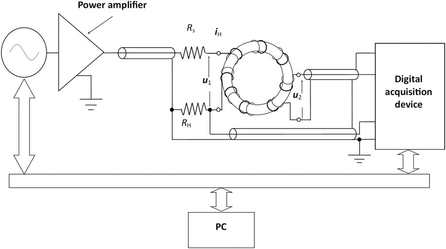
Extensive characterization under controlled sinusoidal and nonsinusoidal induction can actually be achieved with a fluxmetric setup, an example of which is schematically shown in Fig. 3. It is a standard configuration where, with careful control and suppression of the spurious contributions by the stray parameters and taking profit of the broadband capabilities of the used arbitrary function generator, power amplifier, and digital acquisition device, the MHz region on standard ferrite components and tapewound rings can be routinely attained. In a typical arrangement, a Keysight 33220A generator, an NF DC-10 MHz HSA 4101 power amplifier (Keysight Technologies, Santa Rosa, California), and a 500 MHz TDS 724A (Tektronix, Beaverton, Oregon), or HDO 4000 LeCroy (Teledyne LeCroy, Chestnut Ridge, New York), oscilloscope are used. The spurious phase shifts between the measured primary current i H and secondary voltage u 2 are minimized by judicious arrangement of the windings, minimum length of leads and cables, and choice of an anti-inductive shunt resistor R H. The specific detrimental role of this resistor in introducing by stray inductance, a systematic deviation in the measurement of the energy losses at high frequencies, is recognized, as discussed in detail in Ref. Reference Ahmadi, Mazaleyrat, Chaplier, Loyau and LoBue29. It has therefore been suggested that in a number of cases, the direct determination of the power loss by the measurement of the rate of rise of the sample temperature T m upon application of the AC field might be preferable.Reference Loyau, Lo Bue and Mazaleyrat30 In fact, the magnetic power loss per unit mass P is simply related, under adiabatic conditions, to the temperature derivative dT m/dt through the specific heat of the material c p
 $$P = {c_{\rm{p}}}{{{\rm{d}}{T_{\rm{m}}}} \over {{\rm{d}}t}},\quad \left[ {{{\rm{W}} / {{\rm{kg}}}}} \right]\quad .$$
Scheme of a fluxmetric setup used in the broadband measurement of hysteresis loop and losses in soft magnetic materials. The voltage drop u H = R Hi H on the anti-inductive resistance RH, proportional to the applied field, and the secondary voltage u 2 are fed into a high-sampling-rate acquisition device. The prescribed induction waveform is controlled by digital feedback. Number of turns and layout of the primary and secondary windings can evolve with frequency, to guarantee sufficiently high u 2 value at low frequencies and minimum role by the stray parameters at high frequencies.

Equation (2) compares with the standard fluxmetric derivation of the loss per unit volume
 $$P = {1 \over T}\int_0^T {H\left( t \right){{{\rm{d}}B} \over {{\rm{d}}t}}{\rm{d}}t} ,\quad \left[ {{{\rm{W}} / {{{\rm{m}}^3}}}} \right]\quad ,$$
the product of field and induction derivative integrated over the period T = 1/f. The adiabatic conditions can, however, only be emulated, by restraining the loss of heat to the environment. To this end, the sample is generally kept in vacuum. By identifying a heat transmission coefficient K h and formulating a balance equation for the generated, stored and transmitted heat rates upon switch-on of the AC field at time t = 0, we arrive at the equation
 $$P = {{{K_{\rm{h}}}\left( {{T_{\rm{m}}} - {T_0}} \right)} \over {1 - \exp \left( { - {{{K_{\rm{h}}}} \over {{c_{\rm{p}}}}}} \right)t}},\quad \left[ {{{\rm{W}} / {{\rm{kg}}}}} \right]$$
if T 0 is the temperature of the reservoir.Reference Fiorillo31 The coefficient K h is easily determined by fitting the exponential decrease of the sample temperature after switch-off of the field.
Wideband power loss measurements by the thermometric method have been reported for Mn–Zn ferrites in Ref. Reference LoBue, Mazaleyrat and Loyau32. The rise of sample temperature can actually be remarkable, such as to eventually impair, depending on the J p value, the fluxmetric loss measurement at high frequencies. For example, the power loss at 5 MHz and J p = 50 mT in a typical Mn–Zn ferrite sample is of the order of 5 kW/kg, which amounts, according to (2), to a maximum rate of increase of the temperature dT/dt ∼ 7 °C/s. Fast operations and minimum sample heating can possibly be obtained by means of a pulsed field approach.Reference Tellini, Giannetti, Robles and Lizón-Martínez33
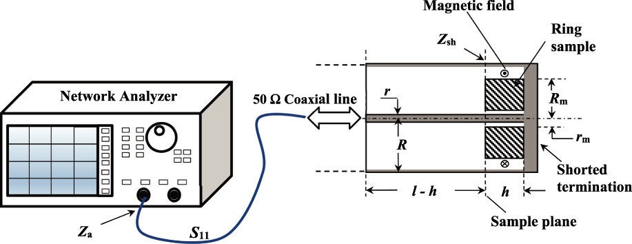
The typical upper frequency limit of a few MHz, intrinsic to the fluxmetric method, does not permit one to perform, in general, a full permeability and loss analysis up to the frequencies where the magnetic response of the materials has, to any practical extent, died out. Under these circumstances, a natural solution for high-frequency characterization is provided by the measurement of the sample impedance using a transmission-line method.Reference Goldfarb and Bussey34 This is quite conveniently performed using a vector network analyzer (VNA), which works both as a variable frequency signal source and as a receiver. With the arrangement shown in Fig. 4, we measure the reflection coefficient S 11(f) of a shorted coaxial line of characteristic impedance Z 0, where a test ring sample is centrally placed at the shorted end of the line. The coefficient S 11(f) at the sample plane is related to the impedance Z sh(f) of the piece of line containing the ring by the equation
 $${Z_{{\rm{sh}}}}\left( f \right) = {Z_0}{{1 + {S_{11}}\left( f \right)} \over {1 - {S_{11}}\left( f \right)}}\quad .$$
The complex magnetic permeability of a ring sample is obtained up to a few GHz by a transmission-line method, making use of a VNA feeding a shorted 50 Ω coaxial cable, which holds the sample at its bottom. The VNA generates a frequency-swept signal and provides the frequency dependence of the complex reflection coefficient S 11(f). This is, in turn, related to the impedance Z sh(f) at the sample plane by the equation Z sh(f) = Z 0(1 + S 11(f))/(1 − S 11(f)), where Z 0 is the characteristic impedance of the line. S 11(f) is measured at the sample plane by moving the port plane via internal software, compensating for the electrical length of the coaxial cable.
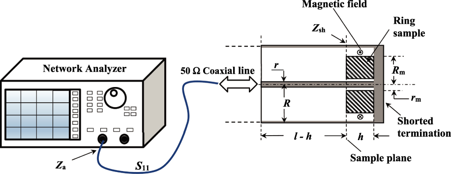
If the sample thickness h is small with respect to the quarter wave length λ/4 of the electromagnetic field, the sample is located in a node of the electric field, and dielectric effects can be ignored. The input impedance Z sh of the piece of line of length h ≪ λ/4 ending into the shorted termination is therefore given by the expression
 $${Z_{{\rm{sh}}}}\left( f \right) = j{Z_0}\tanh \left( {\beta h} \right) \approx j{Z_0}\beta h\quad ,$$
where  $\beta = \omega \sqrt {LC}$ is the propagation constant of the line (the phase variation of the electromagnetic wave per unit length). Since
 ${Z_0} = \sqrt {{L / C}}$, we have Z sh(f) ≈ jωLh. An air-filled lossless coaxial line of radii R and r and length h (Fig. 4) is endowed with field lines concentric with the inner conductor and its impedance is, according to (6), given by the equation
 $${Z_{{\rm{sh}}}} = j\omega {{{\mu _0}} \over {2\pi }}h \cdot \ln {R \over r}\quad .$$
If the same piece of line is filled with a magnetic ring of thickness h, a dissipation term will appear and the material will then be characterized by a complex permeability  $\mu = {\mu _0}{\mu '_{\rm{r}}} - j{\mu _0}{\mu ''_{\rm{r}}}$. The input impedance will be
 $${Z_{{\rm{sh}}}} = j\omega {{{\mu _{\rm{0}}}} \over {2\pi }}\ln {R \over r} \cdot h \cdot \left( {{{\mu '}_{\rm{r}}} - j{{\mu ''}_{\rm{r}}}} \right)\quad ,$$
the resistive part being associated with the magnetic loss. When the ring of radii R m ≤ R and r m ≥ r does not fit the line, Z sh is obtained as the sum of the impedance provided by the region occupied by the material, given by (8) with R m and r m in the place of R and r, and the impedance of the remaining air-filled part. It is essential in this case that the sample be centered in the coaxial line, that is, concentric with the field lines, to avoid demagnetizing effects. Two measurements of Z in,sh are thus performed, with and without the sample inserted in the line. From the difference  $\Delta Z = \Re {\rm{e}}\left\{ {\Delta {Z_{{\rm{sh}}}}} \right\} + j\Im {\rm{m}}\left\{ {\Delta {Z_{{\rm{sh}}}}} \right\}$, the real and imaginary components of the permeability are obtained, according to the equations
 $${\mu '_{\rm{r}}} = 1 + {{\Im {\rm{m}}\left\{ {\Delta {Z_{{\rm{sh}}}}} \right\}} / {\left( {\omega {{{\mu _0}} \over {2\pi }}h \cdot \ln {{{R_{\rm{m}}}} \over {{r_{\rm{m}}}}}} \right)}}\quad {\mu ''_{\rm{r}}} = {{\Re {\rm{e}}\left\{ {\Delta {Z_{{\rm{sh}}}}} \right\}} / {\left( {\omega {{{\mu _0}} \over {2\pi }}h \cdot \ln {{{R_{\rm{m}}}} \over {{r_{\rm{m}}}}}} \right)}}\quad ,$$
together with the related quantities tan δ = μ″/μ′ and Q = 1/tan δ.
At very high frequencies, the condition h ≪ λ/4 may not be fulfilled because the wave length in the material shortens to  ${\lambda _{\rm{m}}} \cong {{{\lambda _0}} / {\sqrt {{{\varepsilon '}_{\rm{r}}}{{\mu '}_{\rm{r}}}} }}$, where
 ${\lambda _0} = {1 / {f\sqrt {{\varepsilon _0}{\mu _0}} }}$ is the free-space wave length and
 ${\varepsilon '_{\rm{r}}}$ is the relative dielectric permittivity. Mn–Zn ferrites display an extremely high DC permittivity, typically of the order of some 105 and, in spite of its rapid decrease with frequency, it might happen that in very large samples λm becomes comparable with h at high frequencies. Consequently, dimensional resonance, in combination with eddy currents, may cause abnormal increase of the loss.Reference Skutt and Lee35 Let us therefore consider a typical Mn–Zn ring sample with h = 5 mm at 1 GHz. At this frequency, we are well beyond the ferromagnetic resonance and
 ${\mu '_{\rm{r}}}$ ∼ 1. By estimating
 ${\varepsilon '_{\rm{r}}}$ ∼ 100 at such frequency, we get λm ∼ 4–8 mm.
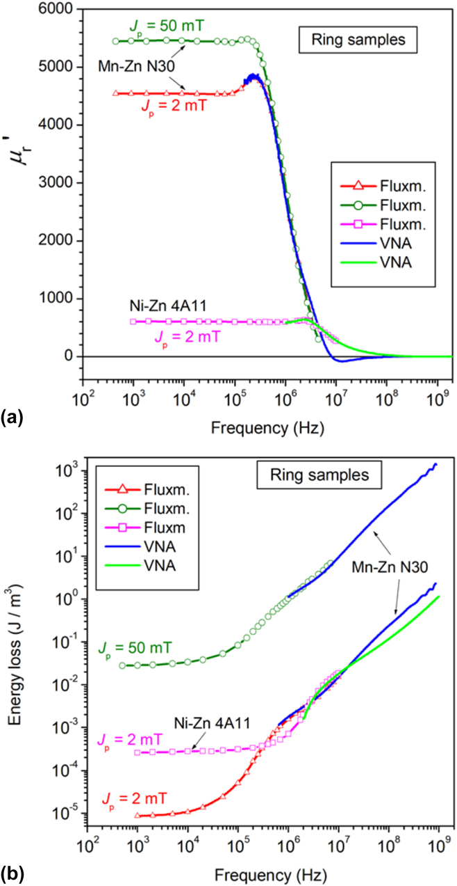
The measured high-frequency μ′(f) and μ″(f) behaviors can be affected to some degree by systematic uncertainty and correction for it may call for a reference sample. Alternatively, one can measure the initial permeability on a lower and partially overlapping frequency interval by the fluxmetric method, for which the measurement uncertainty is known and traceability to the appropriate standards is at hand. What we do, in practice, is to measure fluxmetrically J p up to a few MHz at a defined very low J p value, more or less corresponding to the value expectedly attained at such frequencies by the transmission line measurement on the same ring sample. Obviously, the VNA works at defined incident power (either 1 mW or 10 mW, using the Agilent 8753A; Agilent Technologies, Santa Clara, California), which implies decreasing J p with increasing frequency. We can verify, however, that the involved J p values are generally so low (say, around 1–2 mT and lower at 1 MHz) that μ′(f) and μ″(f) become independent of it in most instances.Reference Magni, Fiorillo, Ferrara, Caprile, Bottauscio and Beatrice36 This could be guessed from the Rayleigh law µ(H) = a + bH at such J p values, where the irreversible contribution bH is much smaller than the reversible permeability a. It is then understood how one can correspondingly obtain the largely overlapping fluxmetric and VNA wideband μ′(f) behaviors shown for a Mn–Zn ring sample in Fig. 5(a). Here, we note that μ′(f) falls, beyond a few hundred kHz, on the VNA measured quantity also at a polarization, as high as J p = 50 mT, which scarcely complies with the notion of initial permeability. This kind of response is typical of the sintered Mn–Zn and Ni–Zn ferrites and of the transverse-anisotropy amorphous and nanocrystalline tapes, where the role of rotations in the permeability behavior is prominent in the low induction range. On approaching the MHz range, the dws become stuck, at least at low inductions, by the dissipative processes and only the rotations provide for the magnetization reversal. In the limit of small oscillations and for isotropically distributed easy axes (e.g., in sintered ferrites), the rotational permeability μrot depends only slightly on J p, at least up to J p/J s ∼ 0.1–0.2. This justifies the observed coalescing of the μ′(f) (and μ″(f)) curves in the upper frequency range and the use of the following expression for the energy loss:
 $$W\left( f \right) = {{\pi J_{\rm{p}}^2\mu ''} / {\left( {{{\mu '}^2} + {{\mu ''}^2}} \right)}}\quad \left[ {{{\rm{J}} / {{{\rm{m}}^3}}}} \right]\quad .$$
(a) Examples of wideband behavior of the relative real permeability µ′r(f) in Mn–Zn and Ni–Zn ferrite ring samples (outside diameter 15 mm, thickness 5.36 mm) at different J p values. The fluxmetric and VNA results overlap in the common frequency interval. (b) Corresponding behavior of the energy losses. The overlapping region shrinks on increasing J p because of a correspondingly increasing proportion of the domain wall processes with respect to the rotations.
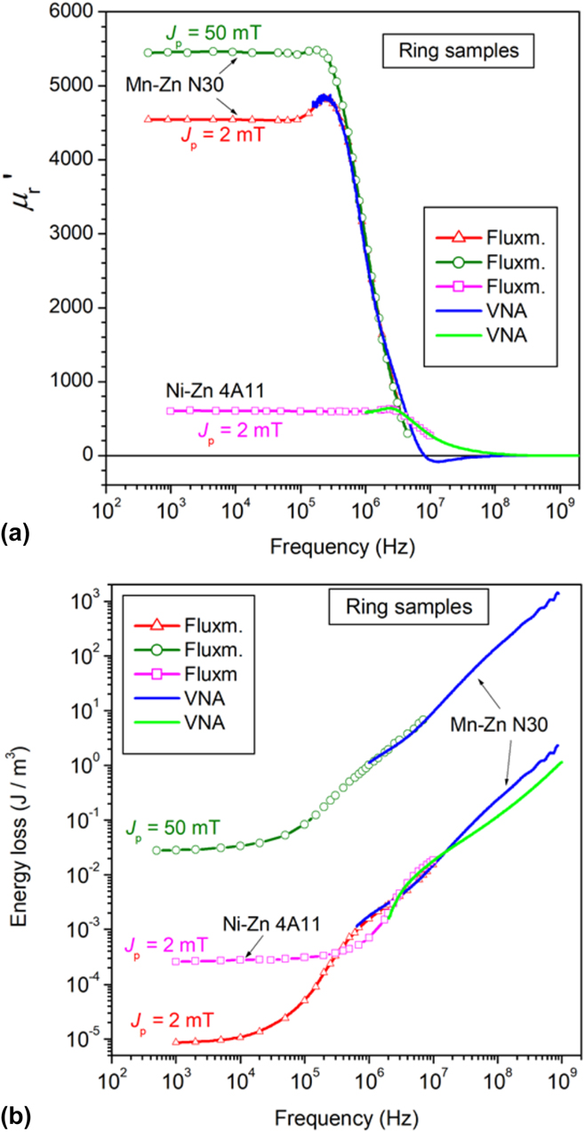
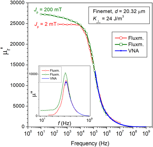
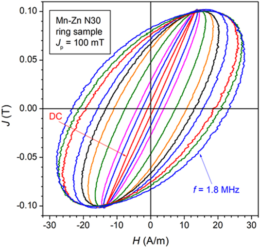
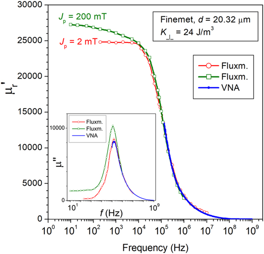
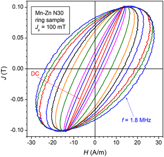
Overlap of the W(f) curves obtained by direct fluxmetric measurements and VNA derived μ′(f) and μ″(f) via Eq. (9) is demonstrated in Fig. 5(b) (N30-type Mn–Zn ferrite). This conclusion equally applies, by virtue of a quasi-linear J(H) curve (see Fig. 1), to the transverse-anisotropy nanocrystalline and amorphous ribbons, up to pretty large J p/J s values. This is shown for a Finemet tape in Fig. 6 and is discussed in Refs. Reference Magni, Fiorillo, Ferrara, Caprile, Bottauscio and Beatrice36 and Reference Beatrice, Dobák, Ferrara, Fiorillo, Ragusa, Füzer and Kollár37. It is fair to stress, in any case, that the experimental limitations of the fluxmetric approach occurring at high frequencies and medium-to-high J p values compound with conceptual hurdles in the definition of complex permeability in strongly nonlinear materials, devoiding (10) of physical meaning. This is what we expect, for example, with extra-soft nanocrystalline or amorphous alloys annealed under longitudinal field, which display rectangular DC hysteresis loops (see Fig. 1). Figure 7 shows, however, that the required approximation of near-elliptical loops holds, for example, for J p = 100 mT (J p/J s ∼ 0.25) in conventional Mn–Zn ferrites.
Real µ′ and imaginary µ″ permeability components versus frequency measured at J p = 2 mT and J p =200 mT in a 20.32 µm thick transverse anisotropy (K ⊥ = 24 J/m3) nanocrystalline ribbon. Fluxmetric and VNA measurements overlap at high frequencies.
Evolution of the hysteresis loops under increasing magnetizing frequency at J p = 100 mT in a N30 Mn–Zn ferrite. The near-elliptical shape of the loops makes realistic their description via the complex permeability.
B. Domain wall dynamics by high-speed Kerr imaging
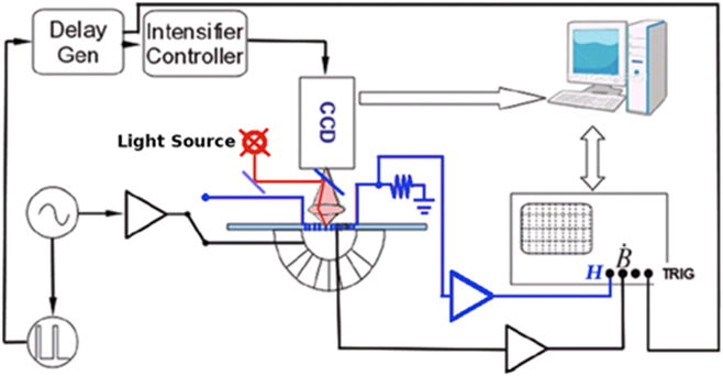
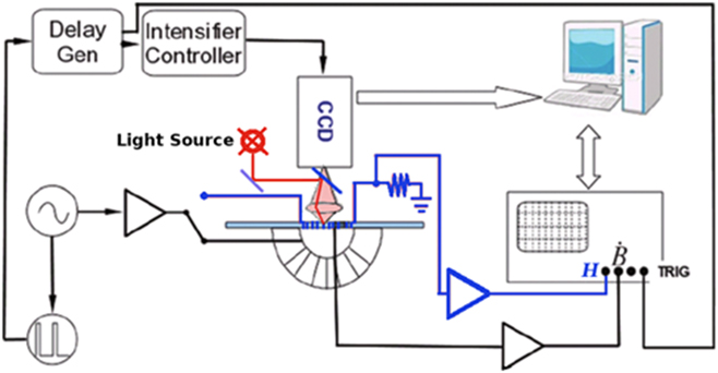
The indirect evidence, arising from the permeability and loss behaviors, of the relative roles of dw displacements and rotations and the eventual disappearance of the former at sufficiently high frequencies, both in ferrites and amorphous/nanocrystalline alloys, becomes manifest in the specific instances where the domains and the dynamics of the dws can be directly observed by Kerr imaging. Amorphous/nanocrystalline strips annealed under a transverse saturating field are endowed with a more or less sharp transverse domain structure, depending on the specifically adopted thermomagnetic treatment and the ensuing value of the induced transverse anisotropy.Reference Flohrer, Schäfer, McCord, Roth, Schultz, Fiorillo, Günther and Herzer38 Under the action of an applied longitudinal field, both dw displacements and rotations occur and can be distinguished by dynamic Kerr measurements. The classical magneto-optical Kerr technique can in fact be extended up to very high frequencies by means of advanced stroboscopic methods,Reference Chumakov, McCord, Schäfer, Schultz, Vinzelberg, Kaltofen and Mönch39 where, under the condition of repeatable domain structure, image acquisition can be made over an extremely short time interval upon a large number of successive cycles. High-speed time-resolved Kerr analysis on strip samples can be carried out, in combination with fluxmetric measurements, with the setup schematically shown in Fig. 8. The strip under investigation, placed between the pole faces of a double-C Mn–Zn ferrite core, is endowed with a small solenoid, exactly fitting the inner diameter of the core, and a few-turn tiny pickup coil, by which the fluxmetric measurements according to the scheme shown in Fig. 3 are made. After removing the upper portion of the double-C yoke and the solenoid, the strip is placed in the focal plane of a wide-field Kerr microscope, based on a Zeiss Axioskop 2 Plus device (Carl Zeiss AG, Oberkochen, Germany). The lower yoke now provides both exciting field and flux-closure. The CCD camera is coupled with a gated image intensifier, placed upon the ocular of the Kerr microscope, ensuring high time resolution, namely apertures as short as 50 ps. The synchronization with respect to the trigger is controlled by a dedicated external delay unit. A circular spot of diameter 1.3 mm with a pixel size of 2.9 µm is illuminated close to the pickup coil. An additional generator, slaved to the field signal generator, synchronously triggers the acquisition of equally time-spaced images along the hysteresis half-loop. The number of averaged acquisitions, ranges from 104 at low frequencies (f < 1 kHz) to 107 for f > 1 MHz. Defocusing due to thermal expansion of the sample poses an upper limit to the combination of high frequencies and high J p values.
Magneto-optical setup for broadband time-resolved observation of the domain structure in amorphous/nanocrystalline strip samples. The core of the setup is an intensified CCD camera, with aperture down to 50 ps, synchronized via an external dedicated delay unit. The specimen, endowed with primary and secondary windings, is placed between the pole faces of Mn–Zn ferrite double-C core for the fluxmetric measurements. After removing the upper portion of the yoke, Kerr measurements are performed (switch in the lower position), with the yoke providing the exciting AC field.
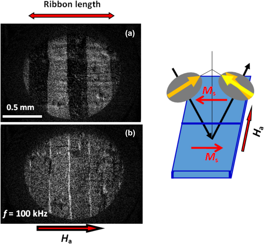
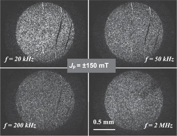
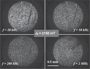
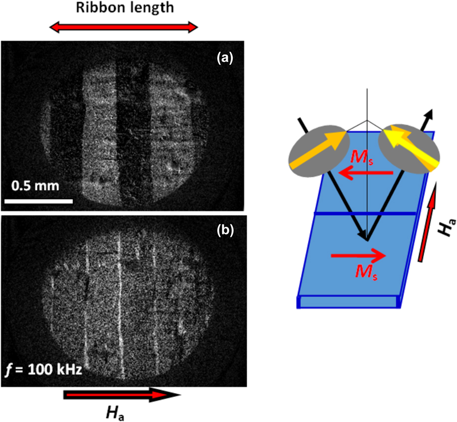
We show in Fig. 9(a) an example of instantaneous domain structure corresponding to a defined value (J, H) of the hysteresis loop in a transverse anisotropy (K ⊥ ∼ 50 J/m3) Co71Fe4B15Si10 ribbon magnetized at 100 kHz and peak polarization J p = 400 mT. The image is the result of an average of about 106 frames and subsequent subtraction of the background (the fully saturated sample). By making the difference of the images taken at +J p and −J p, the area swept by the walls emerges either as a black or white stripe, depending on the direction of motion of the walls [see Fig. 9(b)]. It is noted that parts of the same wall can move in opposite directions. Indeed, although the longitudinally applied field H is basically orthogonal to the 180° dws and its pressure p = 2H·Js on them is nearly zero, the walls are observed to oscillate under alternating H. Close scrutiny on the collective motion of the walls and the measurement of the transverse magnetization variation ΔM ⊥Reference Magni, Bottauscio, Beatrice, Caprile, Ferrara and Fiorillo19 put in evidence that always ΔM ⊥ ∼ 0, implying that what is observed is a simple rearrangement of the dw spacing. Such a process takes place because the rotation of the magnetization modifies the magnetostatic energy content, chiefly at the ribbon edges. Consequently, the system tends to modify the dw configuration, to decrease the free energy. Thus, although ΔM ⊥ ∼ 0 and no contribution to the longitudinal magnetization is provided, a dw related loss is inevitably generated. But the restraining action of the loss related counterfield on the dw motion, depending on the rate of change of the magnetization across the wall, is much higher than the one accompanying the large-scale rotational processes. It turns out that, on increasing the frequency, the dw displacements are increasingly unfavoured and are subject to earlier relaxation with respect to the rotations. The differential dynamic Kerr images in Fig. 10, illustrating the case of a transverse anisotropy Co-based ribbon magnetized between J p = ± 150 mT up to 2 MHz, provide a clear example of increasingly hindered dw motion with increasing frequency. The thin stripes correspond to the difference of the images taken at the tip points of the hysteresis loop and each of them is the trace of the area swept by a moving wall along a half loop. Black and white areas result from the motion of a wall or portions of it along opposite directions, respectively, while the gray background belongs to the sample region where only rotations occur. The shrinking of the stripes with increasing frequency denotes the progressive reduction of the displacements of the dws, which hold still by approaching the MHz region.
Dynamic domain structure observed by high-speed Kerr imaging in a transverse anisotropy (K ⊥ ∼ 50 J/m3) 19 μm thick Co71Fe4B15Si10 amorphous ribbon. (a) The stroboscopic acquisition is made at a given (H, J) point of the hysteresis loop (peak polarization J p = 400 mT) at f = 100 kHz. (b) Differential image where the white stripes emerge from the magneto-optical frames taken at the opposite tip points of the loop and denote the area swept by the walls upon cycling between ±J p. The gray areas are exclusively occupied by the rotational processes.
The dynamic images of the domain structure, taken at J p = ± 150 mT in a transverse anisotropy Co-based amorphous ribbon, are subtracted one to another, to reveal the displacements of the domain walls across the hysteresis loop. The area swept by the walls, exposed by the thin transverse stripes traversing the gray noise background, fully vanish at 2 MHz.

Eddy currents are not the sole responsible for magnetic energy dissipation. In the highly resistive sintered ferrites, their role can even become negligible and spin damping, engendering direct flow of energy by spin wave decay from the precessing spins to the lattice, is invoked. Also in this case, however, the experimental evidence points to early relaxation of the dw motion under increasing frequency.
III. A THEORETICAL ASSESSMENT OF THE BROADBAND MAGNETIC PROPERTIES OF FERRITES AND NANOCRYSTALLINE ALLOYS
The investigation of the soft magnetic materials for high-frequency applications is generally directed at the behavior of two basic technical parameters: initial permeability and magnetic losses. They are not independent quantities and, under the condition of small signal amplitude and defined J p value, they are in a direct relationship, as quantified by Eq. (10). The initial permeability is measured under a very weak field, typically by means of an impedance analyzer, and the J p value is not held constant with frequency. J p is always so small along this measurement that the measured permeability value becomes quite independent of it, the linear approximation holds, and Eq. (10) is fully justified. Under these conditions, the broadband soft magnetic response of the material is qualitatively classified through the Snoek’s product μrDCf 0, where μrDC is the relative DC permeability and f 0 is the cutoff frequency. In soft ferrites, one usually finds that such a product is quite independent of the specific structural properties of the core. This is understood under the assumption that the magnetization process prominently occurs by rotations. For isotropic distribution of easy axes and μrDC ≫ 1, we estimate μrDC f 0 = γJ s/3μ0, where γ is the free-electron gyromagnetic ratio.Reference Stoppels40 However, the landscape of the working conditions of soft cores in present-day electronic applications is too wide for a simple approach based on the initial permeability because we are expected to deal with a range of induction values and waveforms. Consequently, the role of different materials, endowed with a variety of structural properties, very often needs to be assessed upon several frequency decades. The materials of interest can be structurally homogeneous or heterogeneous, and they can either be metallic or poorly conducting and subject to different microscopic dissipation mechanisms. The question is therefore posed, in the absence of a comprehensive theoretical appraisal of their broadband behavior, on how far we can rely on and extend the models developed for the conventional steel sheets used in the electrical machines, that is, for the typical industrial frequencies. A most successful interpretative approach, overcoming the intrinsic limitations of often-adopted empirical descriptions, like the ones based on the Steinmetz’s model, is offered by the statistical theory of losses (STL), a physically grounded model developed for the prediction of the eddy current losses in steel sheets. This model provides solid foundation to the concept of loss separationReference Bertotti41,Reference Bertotti42 and, in combination with the Preisach model of magnetic hysteresis and its dynamic version,Reference Bertotti43 it can be applied, with the help of numerical methods, also in the presence of skin effect using a defined rate-dependent hysteretic constitutive equation.Reference Bertotti, Bottauscio, Chiampi, Fiorillo, Pasquale and Repetto44 But, on proceeding toward the MHz range and further, both with metallic tapes and the poorly conductive/nonconductive ferrites, we should re-adjust to quite a general view of loss separation and loss components. We should account, on the one hand, for energy dissipation by spin relaxation to the lattice, and, on the other hand, for the expected high-frequency evolution of the magnetic constitutive equation.
A. Energy loss and permeability in sintered soft ferrites
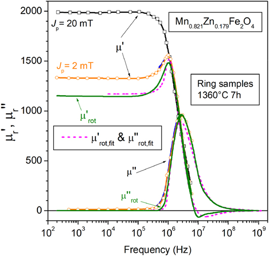
The intrinsic magnetic softness, the low-to-negligible electrical conductivity, the inexpensive raw materials, and the well-established mass production make the sintered low-anisotropy spinel ferrites the material of choice for inductive components destined to broadband applications. But the widespread use of the Mn–Zn and Ni–Zn ferrites is not associated with satisfactory quantitative physical modeling and consensus on role and proportion of the different microscopic mechanisms lying behind the frequency response of permeability and energy losses.Reference Saotome and Sakaki45–Reference Roshen47 The dw displacements and the rotations actually combine and compete in providing the magnetization reversal, and both relaxation and resonant effects have been envisaged for these processes. As shown in Fig. 11, the rotations dominate at low and medium frequencies from the viewpoint of initial permeability (i.e., for J p of few mT). But they are in competition up to high frequencies with the dw displacements from the viewpoint of losses. Rotations can only provide a dynamic contribution to the losses, and even if the dws little contribute to the permeability, they matter in terms of losses at low frequencies since they are the sole dissipative process taking place under quasi-static excitation (area of the DC hysteresis loop). Certain difficulties also exist in Mn–Zn ferrites in treating the evolution of the electrical properties with frequency because the eddy current patterns evolve under increasing f from grain-confined to homogeneously distributed across the sample cross section.Reference Drofenik, Znidarsic and Zajc48
Real and imaginary permeability measured up to 1 GHz by combination of fluxmetric (symbols) and VNA (solid lines) methods in a Mn–Zn ring sample sintered 7 h at 1360 °C. The rotational contributions  ${\mu '_{{\rm{rot}}}}\left( f \right)$ and
 ${\mu ''_{{\rm{rot}}}}\left( f \right)$ are singled out from the measured permeabilities μ′(f) and μ″(f) by a self-consistent procedure, discussed in Ref. Reference Beatrice, Tsakaloudi, Dobák, Zaspalis and Fiorillo55. The dashed lines show the prediction of the
 ${\mu '_{{\rm{rot}}}}\left( f \right)$ and
 ${\mu ''_{{\rm{rot}}}}\left( f \right)$ behaviors by Eq. (15) using the Landau–Lifshitz damping parameter α = 0.04.
It has been suggested in recent times that the STL and the correspondingly derived physical concept of loss separation, where the measured energy loss W(f) is expressed as the sum of hysteresis (quasi-static), excess, and classical components W(f) = W hyst + W exc(f) + W cl(f), can be comprehensively extended to the case where the mechanism of spin damping, alone or in combination with eddy current damping, takes place.Reference Fiorillo, Beatrice, Bottauscio, Manzin and Chiampi49 This amounts to state that these two viscous mechanisms follow strictly similar equations at a mesoscopic level (e.g., at the scale of dws and domains), where the statistical distribution of the locally involved coercive fields regulates the sequence of irreversible processes under an applied field H a(t). It is well known, in fact, and proved by the experiments that a very same equation can describe the dynamics of a wall overcoming the static frictional pressure offered by the coercive field H c in conducting and in insulating single crystalsReference Dillon and Earl50
 $$2{J_{\rm{s}}}\left( {{H_{\rm{a}}} - {H_{\rm{c}}}} \right) = \beta \dot{x}\quad .$$
The damping coefficient β, proportionally relating the pressure of the dynamic field H exc = H a − H c and the wall velocity  $\dot{x}$, is the sum of both eddy currents and spin damping coefficients β = βeddy + βsd. For a rigid isolated wall moving in a slab of conductivity σ and thickness d, the eddy current coefficient is βeddy = 4σJ s2Gd, with the dimensionless coefficient G = 0.1356.Reference Bertotti41 If the slab material is nonconducting, like in the classical experiment by Dillon and Earl on a Mn ferrite single crystal,Reference Dillon and Earl50 the spin damping coefficient becomes βsd = (2J s/μ0γδ)·α, where γ is the electron gyromagnetic ratio, δ is the dw thickness, and α is the Landau–Lifshitz damping constant.Reference Peuzin and du Trémolet de Lacheisserie51 Equation (11) identifies the energy dissipation occurring inside and, with eddy currents, around the moving dw. The coercive field H c is related to the quasi-static energy loss and H exc provides the additional frictional force hindering the wall motion as a whole under dynamic conditions. In particular, the fast microscopic jumps of the dws (the localized Barkhausen reversals) generate both microeddy currents and direct release of energy to the lattice by spin damping and the corresponding energy dissipation per unit volume is W hyst = 4H cJ p. In metallic samples, the localized eddy currents dominate over spin damping, while H exc is related to the eddy currents circulating around the moving dws. Since the experiments of Dillon and Earl show that extra-dissipation proportional to the dw velocity occurs also in the insulating ferrites, we can identify, for both conducting and nonconducting materials, the dw related excess loss W exc = 4H excJ p. Of course, a real sample hosts a multitude of dws and a statistics is required to deal with the great complexity of their motion. As shown by Bertotti,Reference Bertotti41 such a statistics must take into account that the dws generally move in a correlated fashion and one identifies the correlation regions with the term “magnetic objects”. In polycrystalline materials, the grains are reasonably identified with the magnetic objects (MOs).
The local eddy currents obviously diffuse and give rise, according to Maxwell’s equations, to a defined pattern across the sample cross section under steady state. This is the pattern one would predict for an infinitely dense domain structure (or, equivalently, assuming a fictitious structureless material). The correspondingly predicted loss is the so-called classical component, expressed for a bar-like sample of aspect ratio R and cross-sectional area S under sinusoidal flux as
 $${W_{{\rm{cl,eddy}}}}\left( {{J_{\rm{p}}},f} \right) = \left( {{{{\pi ^2}} \over 6}} \right)\sigma '\left( {12k\left( R \right)S} \right)J_{\rm{p}}^2f,\quad \left[ {{{\rm{J}} / {{{\rm{m}}^3}}}} \right]$$
where k(R) is described by an increasing function of R, k(R) = 0.0744R − 0.0434R 2, saturating at the value k(R) = 0.035 for R = 1.Reference de la Barrière, Appino, Fiorillo, Ragusa, Lecrivain, Rocchino, Ben Ahmed, Gabsi, Mazaleyrat and Lo Bue52 In the limit of infinitely extended sheet of thickness d, we obtain 12 k(R)S = d 2 and the standard formula for W cl,eddy(J p, f) is retrieved. Note the use of the real part σ′ of the conductivity in (12). It takes into account the fact that σ can be a complex quantity in a heterogeneous assembly of grains. This is what occurs in the sintered Mn–Zn ferrites, which are composed of semiconducting grains and insulating nanometer thick grain boundaries, electrically behaving as an RC network. While eddy current effects are negligible in the highly insulating Ni–Zn ferrites, sintered Mn–Zn cores are the seat of eddy currents, which circulate inside the grains at low frequencies and progressively invest the whole cross-sectional area of the sample under increasing f.Reference Drofenik, Znidarsic and Zajc48 Consequently, the conductivity is endowed with real and imaginary components, with σ′ monotonically decreasing with f and σ″ passing through a maximum value at intermediate frequencies.Reference Loyau, Wang, LoBue and Mazaleyrat53 With such evolving eddy current patterns, Eq. (12) is applied to the individual grains at low frequencies and to the whole sample cross section at high frequencies, using the grain conductivity and the overall conductivity at high frequencies, respectively.
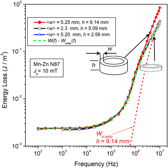
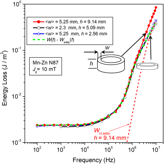
The problem of making a full prediction versus frequency of W cl,eddy(f) in the Mn–Zn ferrites is thus complicated by σ being a complex quantity and by the evolution of the eddy current patterns with frequency. Such a prediction has been provided in recent times, by formulating the electromagnetic field equations through a variational multiscale approach, which leads to a simplified numerical solution.Reference Fiorillo, Beatrice, Bottauscio and Carmi54 This procedure requires, besides knowledge of the sample geometry and grain size, the full electrical characterization of the material up to about 10 MHz. It is remarkable, however, that eddy currents need a sufficiently large sample to play a role and, in most cases, this occurs only by entering the MHz range. This is illustrated by the frequency behavior of the energy loss for J p = 10 mT in N87-type ring samples of different sizes shown in Fig. 12. Up to about 1 MHz, no difference ascribable to the sample size can be put in evidence. Above such a frequency, higher loss is exhibited by the largest ring (5.25 × 9.14 mm2 cross-sectional area), which is due to the eddy current classical contribution W cl,eddy(f), as predicted by the formulation provided in Ref. Reference Fiorillo, Beatrice, Bottauscio and Carmi54.
Magnetic energy loss W(f) up to 10 MHz at J p = 10 mT in commercial Mn–Zn ferrite rings of different sizes. Eddy current losses provide a measurable contribution to W(f) in the largest sample only (thickness 9.14 mm), beyond about 1 MHz, as predicted by the calculated classical loss W cl,eddy(f) (short-dash line).Reference Fiorillo, Beatrice, Bottauscio and Carmi54 By subtracting W cl,eddy(f) from W(f), we obtain the eddy current free loss curve (dashed line), which coincides with the curves measured on the smaller 5.09 and 2.56 mm thick rings.
We might of course verify the possible role by the eddy current related excess loss W exc,eddy(f), which is generated by the motion of the dws simultaneous with the spin damping contribution W exc,sd(f), according to Eq. (11) and the involved damping coefficients βeddy and βsd. Since we deal with granular materials and the motion of the walls and the immediately surrounding eddy currents are basically confined within the grains, we have, according to the STL, βeddy = 4σJ s2G〈s〉, where the average grain size 〈s〉 is typically around 10–50 µm, the grain conductivity σ is about 10–20 Ω−1 m−1, and G = 0.1356.Reference Bertotti41 On the other hand, βsd = (2J s/μ0γδ)·α is quite independent of the structural details and, with γ = 1.76 · 1011 T−1 s−1, a domain wall thickness δ ∼ 1 µm, and α = 0.04, we get βsd ∼ 0.1 J s/m4 versus βeddy ∼ 10−4 J s/m4. The grain conductivity is thus sufficiently low to make W exc,eddy(f) negligible with respect to W exc,sd(f). It is concluded that W exc(f) ≅ W exc,sd(f). We can derive it, by virtue of Eq. (11), closely following the approach of the STL. Following the procedure discussed in Appendix A, we can eventually formulate the excess losses for sinusoidal induction and contribution to the peak polarization by the dws J p,dw < J p
 $$W_{{\rm{exc}}}^{(\sin )}\left( {{J_{{\rm{p,dw}}}},f} \right) = {\left( {{{2\pi } \over 4}} \right)^{{1 \over {1 + m}}}}\lambda \left( m \right){J_{{\rm{p,dw}}}}{\left( {{{{\beta _{{\rm{sd}}}}SV_0^m{J_{{\rm{p,dw}}}}f} \over {\left\langle s \right\rangle J_{\rm{s}}^2}}} \right)^{1/(m + 1)}}\quad \left( {m \le 1} \right),\quad \left[ {{{\rm{J}} / {{{\rm{m}}^3}}}} \right]\quad ,$$
where S is the cross-sectional area of the sample, V 0 is a statistical parameter related to the distribution of the local coercive fields,Reference Bertotti42 and
 $$\lambda \left( m \right) = \int_0^{2\pi } {{{\left| {\cos \varphi } \right|}^{{{(2 + m)} / {(1 + m)}}}}{\rm{d}}\varphi } \quad .$$
As previously remarked, the dw displacements will fully relax in favor of the rotational processes at high frequencies. Consequently, W exc,sd(f) will tend to vanish, following the decrease of J p,dw.
The excess loss in steel sheets is experimentally obtained, as a rule, by subtracting W hyst(J p) and W cl,eddy(J p, f) from the measured energy loss W(J p, f). In the low-anisotropy soft ferrites, however, we need to account for the role of the rotations and the mechanism of damping affecting the magnetic moments that oscillate inside the domains. The oscillation amplitude fluctuates from grain to grain, as imposed by the local value of the anisotropy field, but to incomparably smaller degree than the sharp variations imposed by the full moment transitions occurring inside the moving wall, responsible for W hyst and W exc. The scale of eddy currents generated by the spins rotating inside the domains is thus sufficiently wide to be included in the classical loss component W cl,eddy(J p, f) (Fig. 12). The problem therefore is posed of providing also a formulation for the rotational loss W rot,sd(J p, f) due to the spin damping mechanism. Again, we have to deal with a large-scale effect, bearing resemblance to the classical eddy current loss, and it can similarly be treated separately from the excess loss W exc,sd(J p, f). To this end, we take profit of the quasi-linear behavior exhibited by the soft ferrites up to reasonable J p values (see Fig. 7), of absolute interest for the high-frequency applications. We thus describe the viscous rotational response of the spins in the bulk to the applied AC field by the Landau–Lifshitz–Gilbert equation, which provides a frequency-dependent constitutive magnetic equation of the material in terms of complex rotational susceptibility  ${\chi _{{\rm{rot}}}}\left( f \right) = {\chi '_{{\rm{rot}}}}\left( f \right) - j{\chi ''_{{\rm{rot}}}}\left( f \right)$. It is shown in Appendix B that the real and imaginary susceptibility components, averaged over the distribution g(H k,eff) of the amplitude of the anisotropy field H k and the orientation of the easy axes in the single grains, can be expressed as
 $$\left\langle {{{\chi '}_{{\rm{rot}}}}\left( f \right)} \right\rangle = {2 \over 3}\int_0^\infty {g\left( {{H_{{\rm{k,eff}}}}} \right){{\chi '}_{{\rm{rot}}}}\left( {f,{H_{{\rm{k,eff}}}},{\pi \over 2}} \right){\rm{d}}{H_{{\rm{k,eff}}}}\quad ,}$$
 $$\left\langle {{{\chi ''}_{{\rm{rot}}}}\left( f \right)} \right\rangle = {2 \over 3}\int_0^\infty {g\left( {{H_{{\rm{k,eff}}}}} \right){{\chi ''}_{{\rm{rot}}}}} \left( {f,{H_{{\rm{k,eff}}}},{\pi \over 2}} \right){\rm{d}}{H_{{\rm{k,eff}}}}\quad ,$$
if 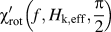 ${\chi '_{{\rm{rot}}}}\left( {f,{H_{{\rm{k,eff}}}},{\pi \over 2}} \right)$ and
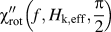 ${\chi ''_{{\rm{rot}}}}\left( {f,{H_{{\rm{k,eff}}}},{\pi \over 2}} \right)$ are the solutions at the frequency f of the Landau–Lifshitz equation for anisotropy field of strength H k,eff orthogonal to the exciting AC field. An example of predicted rotational permeabilities
 ${\mu '_{{\rm{rot}}}}\left( f \right) = 1 + \left\langle {{{\chi '}_{{\rm{rot}}}}\left( f \right)} \right\rangle$ and
 ${\mu ''_{{\rm{rot}}}}\left( f \right) = \left\langle {{{\chi ''}_{{\rm{rot}}}}\left( f \right)} \right\rangle$ is given in Fig. 11. With such a prediction, we identify an average value for the anisotropy field, that is, for the effective average anisotropy constant of the material. As discussed in Appendix B, the rotational energy loss is then calculated as
 $${W_{{\rm{rot}}}}\left( f \right) = {{\pi J_{\rm{p}}^2{{\mu ''}_{{\rm{rot}}}}} / {\left( {{{\mu '}^2} + {{\mu ''}^2}} \right)}}\quad \left[ {{{\rm{J}} / {{{\rm{m}}^{\rm{3}}}}}} \right]\quad ,$$
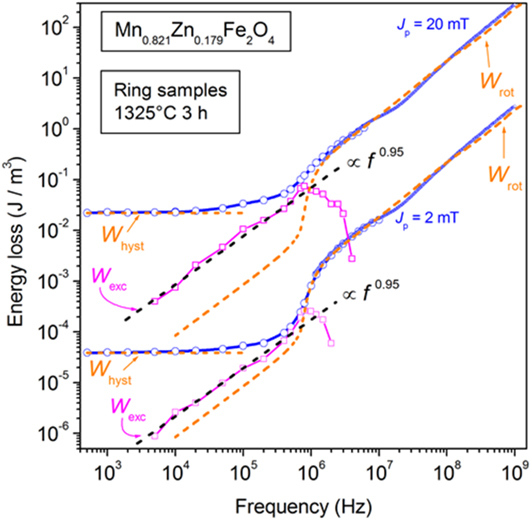
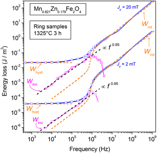
where μ′ = μ′dw + μ′rot and μ″ = μ″dw + μ″rot. The calculated W rot(f) curves are shown in Fig. 13 for J p = 2 mT and J p = 20 mT, compared with the experimental W(f) curves of a Mn0.821Zn0.179Fe2O4 ring sample of cross-sectional area S = 2.6 × 1.2 mm2. With thickness d = 1.2 mm, eddy current effects are negligible and we can proceed to the loss decomposition according to W(f) = W hyst + W exc(f) + W rot(f). The so-obtained W exc(f) is shown to depend on frequency according to the power law W exc(f) ∝ f p, with p = (1/(1 + m)) ∼ 0.95, that is, m ∼ 0.05 in Eqs. (13) and (14). Physically, this implies, according to the STL, a narrow distribution of the local coercive fields and weak increase with frequency of the MOs (or dws) active at a given instant of time. The polycrystalline ferrite aggregate lacks in fact the homogenizing effect of eddy currents and the related mechanisms of dw bowing, instability, and multiplication.
DC-1 GHz energy loss W(f) measured at two J p levels in a Mn–Zn ring sample sintered 3 h at 1325 °C and its decomposition W(f) = W hyst + W exc(f) + W rot(f). The 1.2 mm thick sample is free of eddy current losses. W hyst is an experimental quantity, W rot(f) is calculated by Eq. (16), and W exc(f) is obtained as a difference. W exc(f) significantly contributes to W(f) from some 50 kHz up to about 1 MHz, where it starts to drop (together with W hyst). In this frequency interval, it follows a law of the type W exc(f) ∝ f p, with p ∼ 0.95.
B. Modeling magnetic losses in transverse anisotropy nanocrystalline alloys
The excellent broadband properties of the transverse anisotropy nanocrystalline ribbons are apparent in the example of initial permeability versus frequency behavior provided in Fig. 6, concerning a tapewound ring sample of thickness 20.32 µm endowed with K ⊥ = 24 J/m3. A high value of the Snoek’s product μrDCf 0 = 3.4 × 10⁹ Hz is associated with a residual µ′r ∼ 60 at 100 MHz and a low value of the energy loss at all frequencies, as illustrated in Fig. 2. Similarly good response and frequency behavior can be found in the Co-based amorphous ribbons, whose main physical difference with the nanocrystalline alloys consists in the fairly lower saturation magnetization.Reference Herzer and Buschow8,Reference Fiorillo, Bertotti, Appino, Pasquale and Peterca20 It is remarkable in Fig. 6 the fact that the increase of J p by two orders of magnitude, from 2 to 200 mT, brings about a relatively small increase of the DC permeability, in association with the coalescing of the µ′ versus frequency curves around 50–100 kHz. This behavior descends from the existence of the previously described transverse domain structure, making rotations the dominant magnetization process (as far as permeability is concerned). As shown in Sec. II.B, the dws perform a substantial travel under an applied alternating longitudinal field Ha, although nearly orthogonal to it, the main reason residing in the evolution of the free poles at and close to the ribbon edges. This implies that both hysteresis and the excess losses, exclusively generated by the dw motion, will appear. As the Kerr experiments show, the dw displacements relax, depending on the ribbon thickness, to full extent beyond some 100 kHz and only the rotations are involved in the upper frequency range. This amounts to state that the magnetization process is spatially uniform, if compared to the extreme localization of the dw processes. We are thus under a condition where a classical approach applies and, as shown in Fig. 1, a linear approximation holds so that the DC permeability can play the role of quasi-static constitutive equation. Given the typical resistivity and thickness values of the ribbon samples and the wide range of frequencies, we would expect, according to the solution of the electromagnetic diffusion equation that the skin effect should soon or later enter into play. In such a case, the frequency dependence of the classical loss should pass from the W cl,eddy ∝ f to the W cl,eddy ∝ f 1/2 dependence.Reference Bertotti41 This is never observed.Reference Magni, Bottauscio, Beatrice, Caprile, Ferrara and Fiorillo19 The point here is that the DC permeability is hardly acceptable as constitutive equation at high frequencies.Reference Seemann, Leiste and Bekker56,Reference Serpico, Mayergoyz and Bertotti57 On the other hand, to find a dynamic constitutive equation is not an easy task. In the present case, however, we have to face the rotational process at high frequencies, under favorable geometrical conditions, where the AC field is orthogonal to the easy axis and a simple antiparallel domain structure exists. This permits us to focus on such a process and analytically solve the associated linearized Landau–Lifshitz equation
 $${{\partial {\bi{M}}} \over {\partial t}} = - {\mu _0}\gamma {\bi{M}} \times {{\bi{H}}_{{\rm{eff}}}} + {\bi{M}} \times {\alpha \over {{M_{\rm{s}}}}}{{\partial {\bi{M}}} \over {\partial t}}\quad .$$
We pose Heff = Hk + h and M = Ms + m, where both Hk and Ms lie along the transverse x direction and the dynamic field h and magnetization m are treated as perturbations. The system is conveniently assumed as a single domain, lumping the role of the actual antiparallel domain structure into a demagnetizing coefficient for the z direction, normal to the ribbon plane, N dz < 1 and a demagnetizing field h dem = −N dzm z. m is composed of longitudinal m y and vertical m z components. Finally, the longitudinal effective field h eff,y is the sum of the applied AC field h a and the eddy-current counterfield h eddy.
A solution of Eq. (17) can then be found analytically, within the harmonic approximation, and an expression for the intrinsic susceptibility χint(f), playing the role of a frequency-dependent constitutive magnetic equation of the material, is derived, as demonstrated in detail in Ref. Reference Beatrice, Dobák, Ferrara, Fiorillo, Ragusa, Füzer and Kollár37. Such a quantity is then entered the Maxwell’s diffusion equation, written as
 $${{{\partial ^2}{h_{\rm{y}}}} \over {\partial {z^2}}} = j\omega \sigma {b_{\rm{y}}}\quad ,$$
where b y is the AC induction. This is solved, with the appropriate boundary conditions, in conjunction with the constitutive equation
 $${b_{\rm{y}}} = {\mu _0}\left( {1 + {\chi _{{\mathop{\rm int}} }}\left( f \right)} \right){h_{{\rm{eff,y}}}} = {\mu _{{\mathop{\rm int}} }}{h_{{\rm{eff,y}}}}\quad .$$
As shown in Ref. Reference Beatrice, Dobák, Ferrara, Fiorillo, Ragusa, Füzer and Kollár37, the calculations eventually lead to the following expression for the energy loss, of classical character, associated with the magnetization rotations
 $${W_{{\rm{rot}}}}\left( f \right) = {{\pi B_{\rm{p}}^2} \over {2\left| {{\mu _{{\mathop{\rm int}} }}} \right|}} \cdot {{\left( {\lambda ' - \lambda ''} \right)\sinh \left( {\lambda ' - \lambda ''} \right) - \left( {\lambda ' + \lambda ''} \right)\sin \left( {\lambda ' + \lambda ''} \right)} \over {\cosh \left( {\lambda ' - \lambda ''} \right) - \cos \left( {\lambda ' + \lambda ''} \right)}}\quad ,$$
where λ′ and λ″ are the real and imaginary parts of the complex quantity
 $$\lambda = \lambda ' + j\lambda '' = \sqrt {{{\omega \sigma \left| {{\mu _{{\mathop{\rm int}} }}} \right|{d^2}} \over 2}} \cdot \left( {\sqrt {{{1 + {{{{\mu '}_{{\mathop{\rm int}} }}} / {\left| {{\mu _{{\mathop{\rm int}} }}} \right|}}} \over 2}} - j\sqrt {{{1 - {{{{\mu '}_{{\mathop{\rm int}} }}} / {\left| {{\mu _{{\mathop{\rm int}} }}} \right|}}} \over 2}} } \right)\quad .$$
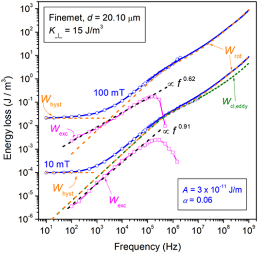
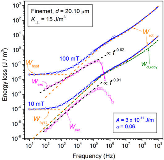
We show in Fig. 14 an example of DC-1 GHz energy loss behavior measured on a 20.1 μm thick tapewound nanocrystalline ring sample endowed with transverse anisotropy K ⊥ = 15 J/m3 and its decomposition into the hysteresis W hyst, rotational W rot(f), and W exc(f) components. It is observed how W rot(f) (dashed line), calculated assuming the exchange stiffness constant value A = 3 × 10⁻¹¹ J/m and the Landau–Lifshitz damping constant α = 0.06, fully covers the experimental W(f) above a few hundred kHz. It is remarked that eddy currents appear to provide larger contribution to W rot(f) than dissipation by spin damping. The excess loss follows a power law dependence on frequency W exc(f) ∝ f p, with the exponent p < 1, decreasing with increasing J p, and drops beyond some 100 kHz, as expected from the predicted and magneto-optically observed relaxation of the dw processes. The decrease of p with J p is understood with a correspondingly increased probability for dw multiplication.
DC-1 GHz energy loss W(f) measured in a 20.1 µm thick transverse anisotropy nanocristalline ribbon (tapewound ring sample) with K ⊥ = 15 J/m3 (symbols and solid lines). The loss decomposition is carried out at two different J p values. The rotational loss W rot(f), calculated with Eq. (20), coincides with the measured loss beyond a few hundred kHz. The contribution by eddy currents is put in evidence for J p = 10 mT. The excess loss W exc(f) = W(f) – W rot(f) – W hyst obeys a power law dependence on frequency W exc(f) ∝ f p, with p < 1 and decreasing with increasing J p.
IV. CONCLUSIONS
Soft ferrites and nanocrystalline alloys owe their remarkable soft magnetic properties to intrinsically low anisotropy energy, prone to manipulation through either calibrated chemistry, like in the Mn–Zn compounds, or magnetothermal treatments, like with nanocrystalline ribbons, by which strength of the anisotropy constant and direction of the easy axis can be regulated. The insulating/semi-insulating properties of the ferrites and the very low thickness of the nanocrystalline ribbons are conducive to excellent broadband permeability and energy loss behavior, fully extending inside the MHz range. In spite of widespread studies and ubiquitous applications, the theoretical/phenomenological assessment of these behaviors has been hardly attained in the literature.
In this paper, we review, after a brief introduction regarding the general physical and magnetic properties of these materials, the main experimental techniques adopted for their characterization upon a range of frequencies extending from DC to hundreds of MHz. Attention is devoted to the traditional fluxmetric measuring method, used up to a few MHz, and the transmission-line method using the VNA, by which the GHz range can be attained. Supporting evidence to the envisaged magnetization mechanisms is provided by dynamic magneto-optical observations of the domain structure, performed by means of a high-speed Kerr setup. A useful combination of low anisotropy properties and early relaxation of the dw processes permits one to achieve frequency continuity and overlapping results on passing from one experimental method to the other, within the peak polarization intervals of interest for the high-frequency applications.
The analysis of the broadband loss and permeability properties is based, on the one hand, on the appraisal of the distinct roles of dw displacements and magnetization rotations and, on the other hand, on a generalized view of the concepts and the formulation of the loss separation, as provided by the STL, where spin damping and eddy currents are identified as concurring dissipation mechanisms. In such a context, the Landau–Lifshitz equation is adopted for the determination of the high-frequency magnetic constitutive equation of the material. One important outcome of this approach is that no evidence exists, both in Mn–Zn ferrites and nanocrystalline ribbons, for the appearance of the skin effect. The thin (∼1 mm) ferrite samples are actually devoid of any eddy current contribution to the loss. Formulations are thus provided for the rotational losses, both in ferrites and in transverse anisotropy nanocrystalline ribbons, by which the high-frequency loss behaviors are predicted and found to be in good agreement with the experiments. The loss decomposition can consequently be carried out and the excess loss component, associated with the dw dynamics both with insulating and conducting materials, is found to follow a power law dependence on frequency, as envisaged by the generalized STL.
Supplementary Material
To view supplementary material for this article, please visit https://doi.org/10.1557/jmr.2018.275.