1 Introduction
The understanding of the spreading or the breakup processes of a drop impacting onto a solid substrate is an area of current active research because of its relevance in a number of technological applications such as coating, cleaning, cooling and combustion (Josserand & Thoroddsen Reference Josserand and Thoroddsen2016). It is known that, at room temperature, drop splashing not only depends on the radius
 $R$
, the impacting velocity
 $V$
, the density
 $\unicode[STIX]{x1D70C}$
, the viscosity
 $\unicode[STIX]{x1D707}$
and the interfacial tension
 $\unicode[STIX]{x1D70E}$
of the liquid, but also on the material properties of the gas, on the gas pressure (Xu, Zhang & Nagel Reference Xu, Zhang and Nagel2005) and on the physicochemical properties of the substrate (Duez et al.
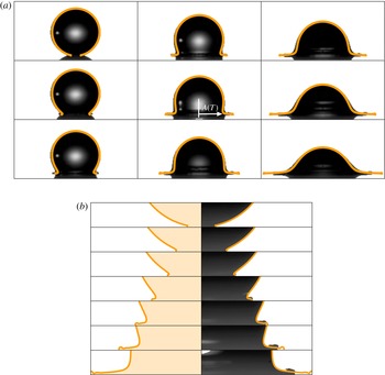
Reference Duez, Ybert, Clanet and Bocquet2007). For the case of drops impacting a smooth and dry solid substrate at room temperature, illustrated in figure 1, it can be observed that once the drop touches the solid at
 $T=0$
, a small bubble – which has no influence on the subsequent dynamics – is entrapped near the axis of symmetry. Subsequently, at the ejection time
 $T_{e}$
, a thin sheet of liquid is expelled from the radial position
 $A(T_{e})$
, with
 $\unicode[STIX]{x03C0}\,A^{2}(T_{e})$
the area of the wetted region. Then, if the impact velocity is below the critical velocity for splashing,
 $V<V^{\ast }$
, the ejected lamella spreads tangentially along the solid; however, if
 $V>V^{\ast }$
, the edge of the liquid sheet dewets the solid as a consequence of the lift forces exerted by the surrounding gas (see Riboux & Gordillo (Reference Riboux and Gordillo2014), hereafter RG14). Then, capillary and Rayleigh–Taylor disturbances grow in the azimuthal direction of the rim, causing its disintegration into drops. At room temperature, splashing will occur only if the liquid front is able to dewet the solid. However, when the temperature of the substrate is above
 $T_{L}$
, with
 $T_{L}$
the Leidenfrost temperature, the liquid never touches the substrate, independent of the value of the impact velocity because under these conditions, the drop levitates on its own vapour (Shirota et al.
Reference Shirota, van Limbeek, Sun, Prosperetti and Lohse2016). Consequently, the critical velocity for splashing will strongly depend on whether the solid temperature is below or above
 $T_{L}$
, as it has been recently reported by Staat et al. (Reference Staat, Tran, Geerdink, Riboux, Sun, Gordillo and Lohse2015). In addition, as a consequence of the frictionless motion of the liquid with the substrate, the maximum spreading diameter of impacting drops increases for temperatures above
 $T_{L}$
with respect to the case of drop impact at room temperature (Lastakowski et al.
Reference Lastakowski, Boyer, Biance, Pirat and Ybert2014; Wilderman et al.
Reference Wilderman, Visser, Sun and Lohse2016).
(a) The sequence of images illustrate an ethanol drop of initial radius
 $R=1.03$
mm impacting against a dry smooth solid surface at room temperature with a velocity
 $V=1.69~\text{m}~\text{s}^{-1}$
–
 $\mathit{We}=\unicode[STIX]{x1D70C}V^{2}R/\unicode[STIX]{x1D70E}=100$
and
 $Re=\unicode[STIX]{x1D70C}VR/\unicode[STIX]{x1D707}=1360$
– at times
 $t\simeq 0$
,
 $t=0.10$
,
 $t=0.19$
,
 $t=0.29$
,
 $t=0.38$
,
 $t=0.48$
,
 $t=0.57$
,
 $t=0.76$
,
 $t=0.95$
with
 $t=TV/R$
. The bright line represents the result of the boundary integral simulation, which is carried out using a number of nodes
 $N$
that increases dynamically in time (
 $N(T=0)=501$
). Nodes are clustered in the regions with the highest curvature. The radius of the wetted area
 $A(T)/R=a(t)=\sqrt{3t}$
(Riboux & Gordillo Reference Riboux and Gordillo2014) is indicated. (b) The right column is a zoom in of the region where the lamella is ejected for different instants of time, namely,
 $t=0.016$
,
 $0.049$
,
 $0.082$
,
 $0.164$
,
 $0.246$
,
 $0.328$
and
 $0.491$
. For reference, the left column illustrates the numerical results for the same values of
 $t$
. The absence of viscous shear stresses causes the rim to flow faster in the numerical simulations than in the experiments.

In this contribution we aim to predict, for temperatures of the substrate above
 $T_{L}$
, the maximum spreading radius of the drop as well as the critical impact velocity above which the drop disintegrates into smaller droplets. Moreover, for impact velocities larger than the critical one, we will also provide results for the velocities and for the diameters of the tiny droplets ejected. For this purpose, the flow field within the ejected lamella is modelled using a ballistic approximation and next, making use of integral balances of mass and momentum, the dynamics of the rim is described. A similar study was carried out by Riboux & Gordillo (Reference Riboux and Gordillo2015) (from now on RG15), where the analytical expressions for the liquid velocity and the height of the liquid sheet deduced in RG14 were used as boundary conditions for the equations describing the flow in the expanding lamella. One of our main contributions here is that these analytical expressions are substituted by universal time-dependent functions calculated numerically using a boundary integral method (BIM). We find that, for short times after impact, the simulations are in excellent agreement with the theoretical predictions in RG14 but, for times
 $T\sim R/V$
, these numerical results depart from those in RG14 and also from the equations provided in Roisman (Reference Roisman2009), Eggers et al. (Reference Eggers, Fontelos, Josserand and Zaleski2010). The differences found are essential to correctly predict the experiments.
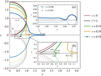
The potential flow numerical results start imposing the initial wetted radius,
 $a=\sin \unicode[STIX]{x1D703}_{0}\approx \unicode[STIX]{x03C0}/36$
with
 $\unicode[STIX]{x1D703}_{0}=5^{\circ }$
. The inset (a) shows the re-gridding procedure used to stabilize the numerical simulation, consisting of placing nodes in between the nodes of the previous time step. The inset (b) is a zoom in of the region from which the lamella is ejected at three different instants of time:
 $t_{e}$
,
 $t=0.15$
and
 $t=0.35$
. The figure also illustrates the wetted radius
 $a(t)$
as well as the radial position of the rim,
 $r_{t}(t)$
, and its velocity,
 $v_{t}(t)$
. The inset also shows the definition of height of the lamella,
 $h(r,t)$
, not to be confused with the width of the rim,
 $h_{t}(t)$
.

Potential flow numerical simulations will be carried out using the BIM described in Rodríguez-Rodríguez, Gordillo & Martínez–Bazán (Reference Rodríguez–Rodríguez, Gordillo and Martínez–Bazán2006), Gordillo & Gekle (Reference Gordillo and Gekle2010). This type of code is adequate to simulate the splashing of drops for substrate temperatures above
 $T_{L}$
since: (i) the vorticity in the falling drop is initially zero and (ii) the shear stresses acting in the circular region of radius
 $A(T)$
below the drop – see figure 1 – are negligible because, in the dynamic Leidenfrost regime, a thin vapour layer prevents the liquid from touching the wall. Therefore, the production of vorticity is restricted to regions near the free surface where the interfacial curvature is highest, e.g. the region where the impacting drop meets the ejected liquid sheet. Consequently, the flow field after the impact is mostly irrotational except in very narrow regions localized near the free surface. Motivated by this fact, in this contribution, we approximate the velocity field within the drop as
 $\boldsymbol{v}=\unicode[STIX]{x1D735}\unicode[STIX]{x1D6F7}$
, with
 $\unicode[STIX]{x1D6F7}$
the velocity potential satisfying the impenetrability condition at
 $Z=0$
,
 $\unicode[STIX]{x2202}\unicode[STIX]{x1D6F7}/\unicode[STIX]{x2202}Z=0$
. In addition, thanks to the symmetry of the flow with respect to the plane
 $Z=0$
,
 $\boldsymbol{v}$
is calculated here as the result of the head on collision of two drops of identical radii
 $R$
moving with respective velocities
 $V\boldsymbol{e}_{z}$
and
 $-V\boldsymbol{e}_{z}$
. Here,
 $\boldsymbol{e}_{z}$
indicates the unit vector pointing in the opposite direction to that of the falling drop. The comparison of the experimental images corresponding to an ethanol drop impacting a solid substrate at room temperature with the numerical profiles is provided in figure 1. Except in the region near the edge of the lamella, the agreement between experiments and numerical results, is remarkable. The discrepancies in the position of the rim observed in figure 1 are due to the fact that, at room temperature, the viscous shear stresses at the wall contribute to further decelerate the advancing front. We used our own experiments, performed at room temperature, to compare with the numerical results since we could not find in the literature experimental images of drops impacting a hot substrate in the Leidenfrost regime with enough spatio-temporal resolution.
2 Potential flow simulations
Following the notation in RG14, lower case variables will be used in what follows to refer to dimensionless variables, which are constructed here using as scales for velocity, length and pressure
 $V$
,
 $R$
and
 $\unicode[STIX]{x1D70C}V^{2}$
, respectively. Since the Froude number
 $\mathit{Fr}=V^{2}/gR\gg 1$
and the shear stresses acting on the liquid are negligible, the only relevant dimensionless parameter characterizing the splashing of droplets in the Leidenfrost regime is the Weber number, defined here as
 $\mathit{We}=\unicode[STIX]{x1D70C}V^{2}R/\unicode[STIX]{x1D70E}$
.
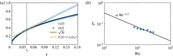
(a) The figure shows the numerical results for both
 $a(t)$
and the radial position of the edge lamella
 $r_{t}(t)$
in the case of
 $\mathit{We}=100$
. The vertical line indicates the ejection time predicted by (2.2) and the dashed line represents the predicted position of the rim, ejected from
 $r=\sqrt{3t_{e}}$
with an initial velocity
 $v_{t}(t_{e})=1/2\sqrt{3/t_{e}}$
, with
 $t_{e}$
given in (2.2). (b) The ejection times predicted by the BIMs are such that
 $t_{e}\propto \mathit{We}^{-2/3}$
, in agreement with (2.2).

The most relevant event taking place after the impact of a drop in the dynamic Leidenfrost regime is that at
 $t_{e}$
, with
 $t_{e}$
the ejection time – see figure 2 – an extremely thin liquid sheet of initial thickness
 $h_{t}(t_{e})$
is expelled tangentially to the substrate with an initial velocity
 $v_{t}(t_{e})$
. In RG14, an algebraic equation for
 $t_{e}$
was deduced based on the following facts: (i) prior to the ejection of the lamella, the time evolution of the radius of the wetted area is
 $a(t)=\sqrt{3t}$
(this result was derived for the very first time by Riboux and Gordillo in RG14 using the linearization of the boundary conditions for the potential flow (Wagner Reference Wagner1932)); (ii) at
 $t_{e}$
, the velocity of the tip of the lamella is equal to the velocity of the wetted radius, i.e.
 $v_{t}(t_{e})={\dot{a}}(t_{e})$
with dots denoting time derivatives; and (iii) the lamella can only be ejected if its tip advances faster than the radius of the wetted area. We concluded in RG14 that
 $t_{e}$
can be calculated solving the algebraic equation
 $$\begin{eqnarray}\displaystyle \frac{\sqrt{3}}{2}\,Re^{-1}\,t_{e}^{-1/2}+\mathit{We}^{-1}=\ddot{a}\,h_{t}^{2}=c^{2}t_{e}^{3/2}\quad \text{with }c=1.1, & & \displaystyle\end{eqnarray}$$
which expresses the fact that the ejection time is the instant at which the deceleration of the edge of the lamella coincides with the deceleration of the wetted area,
 $\ddot{a}$
. For wall temperatures above
 $T_{L}$
, the edge of the lamella is not decelerated by the action of viscous shear stresses and, therefore, setting to infinity the Reynolds number
 $Re$
in (2.1) yields,
 $$\begin{eqnarray}\displaystyle t_{e}=(c^{2}\,\mathit{We})^{-2/3}. & & \displaystyle\end{eqnarray}$$
Using the analytical expressions for both
 $v_{t}(t_{e})$
and
 $h_{t}(t_{e})$
derived in RG14, as well as the result in (2.2), it can be concluded that
 $v_{t}(t_{e})=1/2\sqrt{3/t_{e}}\propto \mathit{We}^{1/3}$
and
 $h_{t}(t_{e})=\sqrt{12}\,t_{e}^{3/2}/\unicode[STIX]{x03C0}\propto \mathit{We}^{-1}$
. Figure 3 confirms the result in (2.2),
 $t_{e}\propto \mathit{We}^{-2/3}$
.
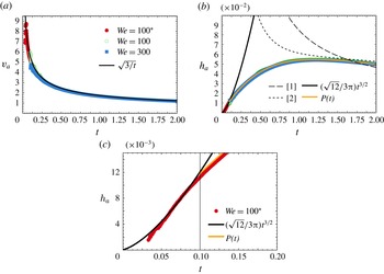
(a) Comparison between the theoretical expression
 $v_{a}=2{\dot{a}}=\sqrt{3/t}$
deduced in RG14 and the numerical result. The good agreement between theory and experiments depicted in this figure is independent of the Weber number whenever
 $\mathit{We}\geqslant 100$
. Two of the simulations shown are carried out using
 $N(T=0)=501$
whereas in the case marked with an asterisk [
 $^{\ast }$
],
 $N(T=0)=1001$
. (b) Comparison of the height of the lamella at
 $r=\sqrt{3t}$
predicted by the models in Eggers et al. (Reference Eggers, Fontelos, Josserand and Zaleski2010) [1] and Roisman (Reference Roisman2009) [2] with the numerical result. (c) Comparison between the theoretical expression
 $h_{a}=h(a(t),t)=(\sqrt{12}/3\unicode[STIX]{x03C0})\,t^{3/2}$
deduced in RG14, valid for
 $t\ll 1$
and the numerical result. The vertical line indicates the instant at which we have set the transition between the result predicted by the potential flow theory and the fitting polynomial
 $P(t)$
in (2.4).

Once the lamella is ejected, as also deduced in RG14, for
 $t>t_{e}$
and
 $t\ll 1$
, both the liquid velocity and the height of the liquid layer at
 $r=a(t)=\sqrt{3t}$
, which is the radial position where the drop meets the lamella, are respectively given by
 $v_{a}=2{\dot{a}}=\sqrt{3/t}$
and
 $h_{a}=\sqrt{12}\,t^{3/2}/(3\unicode[STIX]{x03C0})$
. Figure 4 confirm these theoretical predictions for
 $\mathit{We}\geqslant 100$
. More precisely, figure 4 shows that, while the analytical expression for
 $v_{a}$
is valid for arbitrary times, the corresponding analytical expression for
 $h_{a}$
departs from the numerical results for
 $t\geqslant 0.1$
(see figure 4
c). Therefore, the equations describing the liquid velocity in the lamella
 $u(r,t)$
and its height
 $h(r,t)$
at
 $r=\sqrt{3t}$
i.e. at the radial position from which the liquid sheet is ejected for times
 $t>t_{e}$
, are respectively given by
 $$\begin{eqnarray}\displaystyle \left.\begin{array}{@{}c@{}}\displaystyle u(r=a,t)=v_{a}=\sqrt{3/t},\quad \text{and }\\ \displaystyle h(r=a,t)=h_{a}=\sqrt{12}t^{3/2}/(3\unicode[STIX]{x03C0})\quad \text{for }t<0.1\\ \displaystyle h(r=a,t)=P(t)\quad \text{for }t\geqslant 0.1,\end{array}\right\} & & \displaystyle\end{eqnarray}$$
with
 $$\begin{eqnarray}\displaystyle \left.\begin{array}{@{}c@{}}\displaystyle P(t)=\mathop{\sum }_{i=0}^{5}(0.1p_{i})t^{i}\quad \text{and}\quad p_{0}=-2.453\times 10^{-3},\quad p_{1}=1.321,\quad p_{2}=-1.176,\\ \displaystyle p_{3}=0.4943,\quad p_{4}=-0.1047,\quad p_{5}=8.89\times 10^{-3}\end{array}\right\}\quad & & \displaystyle\end{eqnarray}$$
a polynomial which is fitted to the numerical results.
The ad hoc radial velocity field within the drop proposed by both Roisman (Reference Roisman2009) and Eggers et al. (Reference Eggers, Fontelos, Josserand and Zaleski2010) is
 $u(r,t)=r/(t+\unicode[STIX]{x1D70F})$
, with
 $\unicode[STIX]{x1D70F}$
an adjustable order-unity constant. While the stagnation point type of flow within the impacting drop hypothesized by Roisman (Reference Roisman2009) and Eggers et al. (Reference Eggers, Fontelos, Josserand and Zaleski2010) is a good approximation to the real flow field for
 $t\sim O(1)$
, for times such that
 $t>t_{e}$
,
 $t\ll 1$
, the velocity field at
 $r\simeq \sqrt{3t}$
does not correspond to a stagnation point flow (see RG14 for details). Interestingly, our theory predicts a radial velocity at
 $r=a(t)=\sqrt{3t}$
,
 $u(r=a(t),t)=a(t)/t=\sqrt{3/t}$
for
 $t\ll 1$
which is, by coincidence, the radial velocity corresponding to a stagnation point of flow of the type
 $u=r/t$
particularized at
 $r=\sqrt{3t}$
. This is why figure 4(a) shows a fairly good between the analytical expression
 $v_{a}=\sqrt{3/t}$
and the numerical results for arbitrary values of
 $t$
. Figure 4(b) also shows the values of
 $h_{a}(t)=h(r=\sqrt{3t},t)$
predicted by the model in Roisman (Reference Roisman2009),
 $$\begin{eqnarray}\displaystyle h(r,t)=8\frac{\unicode[STIX]{x1D702}}{(t+\unicode[STIX]{x1D70F})^{2}}\exp \left[-\frac{6\unicode[STIX]{x1D702}\,r^{2}}{(t+\unicode[STIX]{x1D70F})^{2}}\right], & & \displaystyle\end{eqnarray}$$
with
 $\unicode[STIX]{x1D702}=0.39$
,
 $\unicode[STIX]{x1D70F}=2\times 0.25$
and with a constant equal to
 $8$
because here we define dimensionless lengths using the drop radius instead of its diameter, as well as the results predicted by the model in Eggers et al. (Reference Eggers, Fontelos, Josserand and Zaleski2010),
 $$\begin{eqnarray}\displaystyle \left.\begin{array}{@{}c@{}}\displaystyle h(r,t)=\frac{1}{(t+\unicode[STIX]{x1D70F})^{2}}\,H(x)\\ \displaystyle H(x)=\frac{3.19}{(1+C\,x^{2})^{6}}\quad \text{with }\,\,x(r,t)=\frac{r}{t+\unicode[STIX]{x1D70F}},\end{array}\right\} & & \displaystyle\end{eqnarray}$$
with
 $C=0.604$
and
 $\unicode[STIX]{x1D70F}=1$
(Lastakowski et al.
Reference Lastakowski, Boyer, Biance, Pirat and Ybert2014). Clearly, neither the model by Roisman (Reference Roisman2009) not that by Eggers et al. (Reference Eggers, Fontelos, Josserand and Zaleski2010) are in agreement with the numerical results.
3 Prediction of the critical Weber number for splashing and of the maximum spreading radius for droplets impacting in the Leidenfrost regime
For a given instant of time
 $t>t_{e}$
, the lamella extends from the position where the drop meets the liquid sheet i.e.
 $r=\sqrt{3t}$
, down to
 $r=r_{t}(t)$
, with
 $r_{t}(t)$
indicating the radial position of the rim. In RG15, we showed that both the liquid velocity
 $u(r,t)$
and the height of the liquid layer within the lamella,
 $h(r,t)$
, can be calculated using the pair of equations (Gordillo & Gekle Reference Gordillo and Gekle2010; Villermaux & Bossa Reference Villermaux and Bossa2011),
 $$\begin{eqnarray}\displaystyle \frac{\text{D}u}{\text{D}t}=0\quad \text{and}\quad \frac{\text{D}\ln (rh)}{\text{D}\,t}=-\frac{\unicode[STIX]{x2202}\,u}{\unicode[STIX]{x2202}\,r}, & & \displaystyle\end{eqnarray}$$
with
 $\text{D}/\text{D}t\equiv \unicode[STIX]{x2202}/\unicode[STIX]{x2202}\,t+u\,\unicode[STIX]{x2202}/\unicode[STIX]{x2202}r$
the material derivative. The former of the two equations in (3.1a,b
) expresses that fluid particles conserve their velocities within the lamella from
 $r=\sqrt{3t}$
down to the radial position
 $r_{t}(t)$
where the rim is located; the latter is the continuity equation. The pair of equations in (3.1a,b
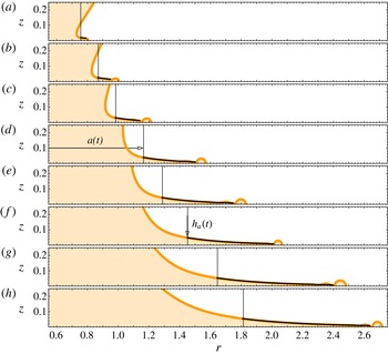
) representing the ballistic motion of fluid particles along the lamella are solved subject to the initial conditions given in equation (2.3) by means of the Lagrangian numerical method already used in RG15. The results of the model for
 $h(r,t)$
, shown in figure 5, are in excellent agreement with the numerical simulations.
Comparison, for
 $\mathit{We}=100$
, between the height of the lamella predicted by the model – ballistic equations (3.1a,b
) subjected to the boundary conditions given in (2.3) – and the numerical result. The vertical line illustrates the radial position
 $r=a(t)=\sqrt{3t}$
for several instants of time as well as the height of the lamella at
 $r=\sqrt{3t}$
,
 $h_{a}(t)=h(r=\sqrt{3t},t)$
;
 $v_{a}$
is the liquid velocity at
 $r=a(t)=\sqrt{3t}$
, namely
 $v_{a}=u(r=\sqrt{3t},t)$
. (a)
 $t=0.19$
, (b)
 $0.25$
, (c)
 $0.32$
, (d)
 $0.45$
, (e)
 $0.55$
, (f)
 $0.70$
, (g)
 $0.90$
and (h)
 $t=1.10$
.

The radial position of the edge of the lamella,
 $r_{t}(t)$
, as well as its thickness,
 $h_{t}(t)$
, are deduced by applying the integral balances of mass and momentum at the rim (Taylor Reference Taylor1959; Culick Reference Culick1960),
 $$\begin{eqnarray}\displaystyle \left.\begin{array}{@{}c@{}}\displaystyle \frac{\text{d}r_{t}}{\text{d}t}=v_{t},\\ \displaystyle \frac{\unicode[STIX]{x03C0}}{4}\frac{\text{d}h_{t}^{2}}{\text{d}t}=[u(r_{t},t)-v_{t}]h(r_{t},t),\\ \displaystyle \frac{\unicode[STIX]{x03C0}\,h_{t}^{2}}{4}\frac{\text{d}v_{t}}{\text{d}t}=[u(r_{t},t)-v_{t}]^{2}\,h(r_{t},t)-2\,\mathit{We}^{-1}.\end{array}\right\} & & \displaystyle\end{eqnarray}$$
The system of equations (3.2) is solved subjected to the following initial conditions,
 $$\begin{eqnarray}\displaystyle \left.\begin{array}{@{}c@{}}\displaystyle r_{t}=a(t_{e})=\sqrt{3\,t_{e}},\\ \displaystyle v_{t}=v_{t}(t_{e})=1/2\sqrt{3/t_{e}},\\ \displaystyle h_{t}=h_{t}(t_{e})=\sqrt{12}\,t_{e}^{3/2}/\unicode[STIX]{x03C0},\end{array}\right\} & & \displaystyle\end{eqnarray}$$
with
 $t_{e}$
given by (2.2).
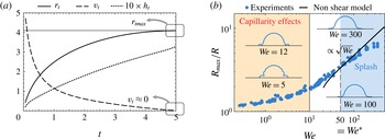
Figure 6(a) shows the solution of the system of equations (3.1a,b
)–(3.3) for a particular value of the Weber number, whereas figure 6(b) illustrates the comparison between the predicted maximum spreading radius and the experimental data in Tran et al. (Reference Tran, Staat, Prosperetti, Sun and Lohse2012). As was pointed out in Wilderman et al. (Reference Wilderman, Visser, Sun and Lohse2016), there are two clearly differentiated regions in the plot
 $r_{max}$
versus
 $\mathit{We}$
of figure 6(b): the impact is elastic for
 $\mathit{We}\lesssim 10$
since the initial kinetic energy is transformed into surface energy, as it apparent from the capillary waves developing at the interface of the impacting drop whereas, for
 $\mathit{We}\gtrsim 10$
, the drop spreading process is dominated by inertia. It is discussed in Wilderman et al. (Reference Wilderman, Visser, Sun and Lohse2016) that approximately one-half of the initial kinetic energy is dissipated in the sudden expansion connecting the liquid sheet with the rim for
 $\mathit{We}\geqslant 10$
, a fact which is implicitly taken into account in the mass and momentum conservation equations (3.2). In spite of the fact that the system of equations (3.2) is analogous to that used in Roisman (Reference Roisman2009), Eggers et al. (Reference Eggers, Fontelos, Josserand and Zaleski2010), Villermaux & Bossa (Reference Villermaux and Bossa2011) and Lastakowski et al. (Reference Lastakowski, Boyer, Biance, Pirat and Ybert2014), the crucial difference between the present study and previous ones is that, in our case, we do not impose a specific form for the velocity field within the lamella. Instead, since fluid particles conserve their velocities within the liquid sheet, our system of equations (3.2) subjected to the real initial conditions given in (2.3), with
 $t_{e}$
calculated self-consistently through equation (2.2), provides us with the correct expressions for both the liquid velocity
 $u(r_{t})$
and the height of the lamella
 $h(r_{t})$
upstream of the toroidal rim, as can be inferred from the good agreement existing between experiments and predictions depicted in figure 6(b).
(a) Radial position
 $r_{t}$
, velocity
 $v_{t}$
and height
 $h_{t}$
of the edge of the lamella as function of the dimensionless time
 $t$
for
 $\mathit{We}=150$
. The maximum spreading radius is reached when
 $r_{t\,max}=R_{max}/R\;\Longleftrightarrow \;v_{t}\approx 0$
. (b) The predicted maximum spreading radius is of the form
 $R_{max}/R\propto \mathit{We}^{1/2}$
for
 $\mathit{We}\gtrsim 20$
. The experiments in Tran et al. (Reference Tran, Staat, Prosperetti, Sun and Lohse2012) are plotted for comparison. Two different regimes are observed: for Weber numbers
 $\mathit{We}\lesssim 10$
, capillary waves develop, distorting the initial shape of the drop, whereas for
 $\mathit{We}>10$
, the impact is dominated by inertia. The black line represents the maximum spreading radius resulting from the self-consistent theory presented here.

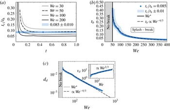
(a) Ratio
 $t_{c}/t_{h}$
as function of
 $t$
for several values of the Weber number. The theory in RG15 predicts the disintegration of the toroidal rim when
 $0.075\leqslant t_{c}/t_{h}\leqslant 0.095$
(area coloured in blue). Therefore, the predicted critical Weber number is
 $\mathit{We}^{\ast }\simeq 50$
. (b) For
 $\mathit{We}>\mathit{We}^{\ast }$
, the rim breaks at
 $t_{b}\propto \mathit{We}^{-4/3}$
. (c) The diameters and velocities of the droplets ejected for
 $\mathit{We}>\mathit{We}^{\ast }$
calculated numerically are approximated here as
 $d_{d}=h_{t}(t_{b})\propto \mathit{We}^{-4/3}$
and
 $v_{d}=v_{t}(t_{b})\propto \mathit{We}^{2/3}$
respectively.

Another of the advantages of not imposing an ad hoc velocity field within the lamella rests in the fact that both the critical Weber number and the diameters and the velocities of the droplets ejected for impact velocities
 $V>V^{\ast }$
, which strongly depend on
 $h(r_{t})$
, can be calculated self-consistently. Indeed, in RG15, following the ideas in Villermaux & Bossa (Reference Villermaux and Bossa2011) and Agbaglah, Josserand & Zaleski (Reference Agbaglah, Josserand and Zaleski2013), we deduced a criterion for the disintegration of the edge of the liquid sheet based on the fact that the droplets composing the spray result from the amplification in the azimuthal direction of Rayleigh–Taylor and capillary instabilities. The growth rates of the disturbances developing in the azimuthal direction of the toroidal rim are highly attenuated as a consequence of the simultaneous growth of its thickness. In consequence, we concluded that drops will only be ejected when the time characterizing the radial growth of the rim,
 $T_{h}=(R/V)t_{h}=(1/H_{t}\,\text{d}H_{t}/\text{d}T)^{-1}$
, is substantially larger than the capillary time
 $T_{c}=(R/V)t_{c}=(\unicode[STIX]{x1D70C}\,H_{t}^{3}/8\unicode[STIX]{x1D70E})^{1/2}$
. The breakup time
 $t_{b}$
is fixed at the instant at which
 $t_{c}/t_{h}\simeq 0.085$
for the reasons explained in RG15, which are reproduced here for the sake of clarity: (i) the characteristic time of growth of a capillary instability is
 ${\sim}3\,T_{c}$
, (ii) a Rayleigh’s stability analysis of capillary perturbations reveals that the dimensionless wavenumber
 $k$
with a fastest growth rate is
 $k=\unicode[STIX]{x03C0}H_{t}/\unicode[STIX]{x1D706}\simeq 0.7$
, where
 $\unicode[STIX]{x1D706}$
indicates the wavelength of the perturbation, which is kept constant in time and (iii) the growth of capillary instabilities is inhibited for
 $k\geqslant 1$
(Eggers & Villermaux Reference Eggers and Villermaux2008). Therefore, in order for capillary corrugations with characteristic initial wavenumbers
 $k=0.7$
to be amplified up to the point that drops are ejected from the rim, it is necessary that, in a time
 $3\,T_{c}$
,
 $\unicode[STIX]{x1D6E5}k<0.3$
or, equivalently, that
 $(\text{d}H_{t}/\text{d}T)\times 3T_{c}\lesssim 0.3H_{t}\Rightarrow T_{c}/T_{h}\lesssim 0.1$
, a value which is very close to
 $t_{c}/t_{h}\simeq 0.085$
.
It is depicted in figure 7(a) that the ratio
 $t_{c}/t_{h}$
is above the threshold
 $0.085$
for
 $\mathit{We}\lesssim 50$
, a fact meaning that the drop never splashes for values of the Weber number, based on
 $R$
, below 50. Therefore, the critical Weber number predicted by our approach is
 $\mathit{We}^{\ast }=50$
, a value which is rather close to the experimental one reported in Staat et al. (Reference Staat, Tran, Geerdink, Riboux, Sun, Gordillo and Lohse2015), who find that
 $\mathit{We}^{\ast }$
based on
 $R$
slightly varies with temperature within the range
 $\mathit{We}^{\ast }\simeq 55{-}100$
. Let us point out that
 $\mathit{We}^{\ast }$
is insensitive to the specific value chosen for the threshold
 $t_{c}/t_{h}$
, whenever this value is included within the range
 $0.075\leqslant t_{c}/t_{h}\leqslant 0.095$
(see the shaded region in figure 7). For values of the Weber number above the critical, figure 7(b) shows that the dimensionless breakup time decreases with
 $\mathit{We}$
as
 $t_{b}\propto \mathit{We}^{-3/4}$
and, motivated by the good agreement existing between experiments and theory reported in RG15, the diameters and the velocities of the tiny droplets ejected radially outwards from the toroidal rim are calculated respectively as
 $d_{d}=h_{t}(t_{b})$
and
 $v_{d}=v_{t}(t_{b})$
. The numerical values for both
 $d_{d}\propto \mathit{We}^{-4/3}$
and
 $v_{d}\propto \mathit{We}^{2/3}$
, which need experimental validation, are provided in figure 7(c).
4 Conclusions
In this contribution we have developed a self-consistent theory to predict the critical Weber number for splashing,
 $\mathit{We}^{\ast }$
, when droplets impact against a solid substrate heated above the dynamic Leidenfrost temperature,
 $T_{L}$
(Tran et al.
Reference Tran, Staat, Prosperetti, Sun and Lohse2012, Reference Tran, Staat, Susarrey–Arce, Foertsch, van Houselt, Gardeniers, Prosperetti, Lohse and Sun2013). Our theory is based on the fact that, in the dynamic Leidenfrost regime, the viscous shear stresses acting on the bottom of the drop can be neglected thanks to the vapour layer preventing the liquid drop from touching the substrate. Therefore, the velocity field within the lamella, which is ejected radially outwards and tangentially to the substrate from
 $r=\sqrt{3t}$
for times after impact
 $t>t_{e}$
, with
 $t_{e}$
the ejection time, can thus be described by means of a ballistic approach. In contrast with previous studies (Roisman Reference Roisman2009; Eggers et al.
Reference Eggers, Fontelos, Josserand and Zaleski2010; Villermaux & Bossa Reference Villermaux and Bossa2011) we do not impose a specific form for the velocity field within the lamella. Instead, since fluid particles conserve their velocities within the liquid sheet, we impose as boundary conditions for the ballistic equations describing the flow in the lamella the numerical results obtained using a BIM code. These boundary conditions agree well with the expressions deduced in RG14 in the limit
 $t\ll 1$
. Once the flow in the lamella is calculated, both the position and the diameter of the edge of the liquid sheet are determined using integral balances of mass and momentum (Taylor Reference Taylor1959; Culick Reference Culick1960). The maximum spreading radius of drops impacting in the dynamic Leidenfrost regime are then calculated in a self-consistent manner, and the results obtained are in good agreement with the experimental data provided in Tran et al. (Reference Tran, Staat, Prosperetti, Sun and Lohse2012). Making use of the fact that drops will only be ejected from the rim when the time characterizing the radial growth of the edge of the lamella is substantially larger than the capillary time, we conclude that
 $\mathit{We}^{\ast }\simeq 50$
. This value is also in good agreement with the experimental values reported in Staat et al. (Reference Staat, Tran, Geerdink, Riboux, Sun, Gordillo and Lohse2015). For
 $\mathit{We}>\mathit{We}^{\ast }$
, using the approach described in RG15, we also provide closed expressions for the diameters and for the velocities of the droplets composing the spray as a function of the Weber number. These expressions need experimental validation.
Acknowledgements
This study has been financially supported by the Spanish MINECO under Project DPI2014-59292-C3-2-P, partly financed through European funds.