I. Introduction
This paper aims at identifying the determinants of Romanian wine companies’ exports and analyzing the link between exports and financial performanceFootnote 1 in the Romanian wine industry.
With 175,000 ha, Romania has Europe's fourth largest vineyard area (behind Spain, Italy, and France). However, due to its relatively low yields, Romania's wine production ranks only seventh in Europe (behind Italy, France, Spain, Germany, Portugal, and Russia) (Anderson and Pinilla, Reference Anderson and Pinilla2018). In addition, Romania's wine production is characterized by an outstandingly high degree of fragmentation. There are approximately 855,000 vineyard holdings in Romania, more than anywhere in Europe (Eurostat, 2020), which, in turn, results in the smallest average vineyard size per holding in Europe.Footnote 2
With an annual volume of approximately 23 million liters (2019), worth US$35 million (Comtrade, 2020), Romania's wine exports are relatively small. Among the world's wine exporting countries, Romania is ranked number 36 by value and 22 by volume (Comtrade, 2020). Approximately 75% of Romanian wine exports by volume are bottled; its main export markets are Germany, the United Kingdom, and The Netherlands.
Our paper analyzes the impact of exports on the financial performance of Romanian wine producers. For this purpose, we use a panel data approach with a sample that includes 207 active companies over the period 2009–2017. Our results suggest that exports are positively linked to financial firm performance and that trade is impacted by several regionalFootnote 3 variables (e.g., wine production per hectare, cultivated vineyard area, agglomeration effects, and growing temperatures). Moreover, exports seem to be higher in regions that specialize in the production of red wine.
The remainder of our paper is organized as follows. Section II presents the literature. Section III describes the methodology and data, and Section IV reports the empirical results. Section V evaluates the results with various robustness checks. Section VI concludes.
II. Literature Review
The literature on exports and economic performance at the micro-level goes back to Bernard and Jensen (Reference Bernard and Jensen1995). By drawing on longitudinal data for U.S. companies, they compare exporters and non-exporters. Exporters generally perform better than non-exporters in the short term, which is due to factors such as firm size, yields, and capitalization. Melitz (Reference Melitz2003) explores the probability of exporting, under different sunk costs and yield levels in a dynamic industry model with heterogeneous firms. He finds that more productive companies can penetrate the export market, while less productive ones continue to operate at the domestic level. Moreover, he shows that, among companies with low yields, the ones with the lowest yields are eventually forced to leave the market. Crozet, Head, and Mayer (Reference Crozet, Head and Mayer2012) provide further support to Melitz's (Reference Melitz2003) analysis as they develop an empirical analysis that uses data on products’ quality in a study that investigates the French wine industry. They conclude that higher wine quality levels increase exports to more markets, as well as drive up prices and sales in each market.
A series of studies have followed these papers. They consider either yields or profitability to capture firm performance in relation to exports.Footnote 4 Within this framework, two strands of literature can be identified. The first strand shows a positive impact of exports on profitability (Fryges and Wagner, Reference Fryges and Wagner2010), while the second one finds mixed results (either a negative impact (Esen, Simdi, and Erguzel, Reference Esen, Simdi and Erguzel2016), non-linear effects (Vogel and Wagner, Reference Vogel and Wagner2010), or no connection between exports and financial performance (Wagner, Reference Wagner2012).
Only a few papers are strictly devoted to wine, with many focusing on France. For example, by analyzing the French wine industry, Viviani (Reference Viviani2009) finds that exports positively influence financial performance, but through the intangible expenses directly connected with companies’ profit and risk. Similar results are put forward by Amadieu, Maurel, and Viviani (Reference Amadieu, Maurel and Viviani2013), also for France. They show that exports improve financial performance, but the intensity of the effect depends on whether the wine producer is a corporation or a cooperative. Unlike the aforementioned authors, Cardebat and Figuet (Reference Cardebat and Figuet2019) test the influence of the exchange rate as the main determinant for French wine exports. An Armington panel model, covering 2000 to 2011, represents the empirical support. The finding shows that French wines lose in terms of competition during the 2000s: this is explained by the rise of domestic wine prices compared to foreign competitors and the appreciation of the euro with respect to both USD and GBP.
Only a few papers have analyzed the Romanian wine industry assessing its competitiveness (Nakata and Antalis, Reference Nakata and Antalis2013) or the trade performance of the sector (Noev, Reference Noev2007).
Our paper aims at investigating how exports interact with the financial performance of Romanian companies in the wine industry, using an original database and different econometric tools.
III. Data and Methodology
A. Methodology
We analyze the influence of wine exports on financial performance in the Romanian wine industry with a panel model approach and run several regressions from 2009 to 2017, using an original data set, that is, firm-level data for 207 wineries in combination with Google Trends data, and various data at the regional level.
Our empirical strategy consists of two steps: (1) exploring the main determinants of wine exports, and (2) examining the impact of wine exports on financial performance.
(1) Wine Exports and Their Determinants
We employ an ordinary least squares (OLS) panel model and consider yields, vineyard area, an agglomeration index, export prices, and climate conditions (i.e., temperature and precipitations) as exogenous determinants. We conduct our analysis at the firm level and also include various regional NUTS II level data. The model is written as

where Exportsijt denotes the wine exports of company i from region j at moment t. α is the intercept, while βk are the slopes of the independent variables X k (i.e., regional wine yields, vineyard area, agglomeration effect, and climatic conditions), with k = 1 .. n. The error term is ɛ it varying over both companies and time. In order to avoid endogeneity issues, the lag of wine yields is alternatively used in the estimations. We denote each wine variety with a dummy variable. The unobserved heterogeneity is modeled via random-effects. We expect these models to be more appropriate than fixed-effect ones as T < N in our case, and heterogeneity can be considered constant over time. The final selection of the random effects is made based on a Hausman test. Both OLS and generalized least squares (GLS) estimators are considered further in the random effect estimations.
(2) Exports and Financial Performance
We follow a dynamic approach employing a generalized method of moments (GMM) estimator. The GMM approach tackles the endogeneity issue generated by the reverse causality between exports and financial performances, but also caused by omitted variables or measurement errors. Additionally, such estimators allow controlling for heteroscedasticity. Roodman (Reference Roodman2009) underlines several advantages of the GMM estimators. They can be used in the case of “1) ‘small T, large N’ panels, meaning few time periods and many individuals; 2) a linear functional relationship; 3) one left-hand-side (LHS) variable that is dynamic, depending on its own past realizations; 4) independent variables that are not strictly exogenous, meaning that they are correlated with past and possibly current realizations of the error; 5) fixed individual effects; 6) heteroskedasticity and autocorrelation within individuals but not across them” (Roodman, Reference Roodman2009, p. 86).
In our analysis, we acknowledge that the current financial performance of a winery may depend on its past financial performance and on current economic variables. The Arellano and Bond (Reference Arellano and Bond1991) GMM estimator (GMM-dynamic) can be used to capture this. However, a weak instrument problem can occur in the Arellano–Bond approach. To take account of the fact that in this modeling strategy, the lagged levels of regressors might be poor instruments for the first-differenced ones, we finally choose to employ the Blundell and Bond (Reference Blundell and Bond1998) approach. This offers an improved version of the GMM-dynamic estimator, the so-called GMM-system estimator, which also considers the level of variables, as shown in Equation (1). A system with two equations represents the core of the GMM-system estimator: one differenced and another one in level. Hansen's J-test is used to check the validity of instruments, its alternative—the Sargan test—being inconsistent under robust GMM. As Mileva (Reference Mileva2007) suggests, the Arellano–Bond test for autocorrelation allows for the detection of the autocorrelation in residuals by following the AR(2) test in the first difference. Given its superior valence in terms of consistency compared to the GMM-dynamic models, the GMM-system estimator is used in all related estimations for this paper.
Our model can be written as

where φ denotes the coefficient of the lagged dependent variable FinPerf, which, in turn, captures the financial performances of company i at time t. Exports represents the variable of interest (i.e., firms’ exports), while ψ is the coefficient of the vector of control variables X′. The standard random variable with zero mean is captured by νi. The error term is ɛ it, which varies over both country and time.
B. Data
One of the main challenges in analyzing Romanian wine exports is the lack of data. We try to overcome this problem by using firm-level data, Google Trends data, and regional data. Our empirical approach is constructed on an extended unbalanced 207-firm panel covering the period 2009–2017.
The main panel is divided into two sub-panels: we use the first one in the export determinants study (1), and the second in the exports and financial performances analysis (2).
(1) Export Determinants
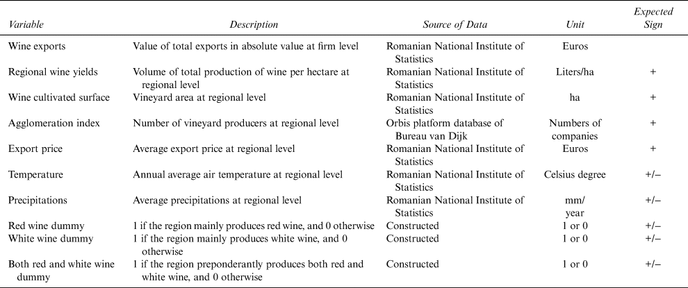
In order to analyze export determinants we include the following variables: wine exports at the firm level, wine yields at the regional level, regional vineyard area, agglomeration index, national export prices, temperature, and precipitation. As each region produces different grape varieties, we also included three dummy variables for predominant wine production, one for each red, white, and both red and white wine varieties produced at the regional level.
The dependent variable is wine exports, measured in euros. Since exports data are unavailable at the firm level, we compute this variable at time t, by multiplying the operational revenues (euros) of a company i from the region r, by the “Google Trends Wine” regional indicator (transformed in percentage), as

The intensity of exports at the regional level, captured through the “Google Trends Wine” indicator, is used to proxy the exports at the level of companies. We suppose that the export intensity at the regional level is related to the operational revenues of a company active in that region to proxy the firm's exports (i.e., the wine exports in operational revenues increase as the intensity of exports at the regional level rises as well).
The “Google Trends Wine” variable is obtained based on the Google Trends Index. It measures the frequency of searches for the English word “wine” in Romania at the regional level. We follow the approach of Askitas and Zimmermann (Reference Askitas and Zimmermann2015), in which different variables in the social sciences can be approximated using internet resources. We assume that wine exports are positively and strongly correlated with the frequency of Google searches for “wine” (i.e., the more searches for “wine,” the higher the wine exports in the area should be). Google Trends Index (2018) searches generate values between 0 and 100, where 0 (or 0% ≈ 0) is the minimum level and 100 (or 100% ≈ 1) is the maximum level. Thus, exports of wine are higher if the indicator is close to 100 ≈ 1. We compute the correlation coefficient of our export index using the Romanian national wine exports data (mill euros),Footnote 5 over the period 2009–2017. The results show that both the “Google Trends Wine” index and the country's wine exports follow the same trend except for 2015–2017. Nevertheless, over 2009–2017, the correlation coefficient between the two variables equals 0.918, which suggests that the “Google Trends Wine” index can serve as a proxy for wine exports. This proxy is simple to compute and allows for collecting data for various periods, frequencies, regions, and companies.Footnote 6
The first three independent variables are average yields in the wine industry at the regional level, the vineyard area in each region, as well as an agglomeration index. The first two are specific determinants for wine exports, according to the Romanian Wine Exporters and Producers Association (WEPA) (2016). The third is a constructed index for each NUTS 2 region, taking into account the number of firms. The average wine yield at the regional level is expressed in liters per hectare; the regional vineyard area is measured in hectares. We compute the agglomeration index as the number of active winemakers per NUTS 2 region. This index is meant to capture the concentration of wine companies in a specific region. All three variables, available at the regional level, are linked to firm-level data since we have the exact geographical location for each company. We expect the regional average wine yields to be positively linked with wine exports. The expected impact of the regional vineyard area on wine exports is ambiguous. Brunow, Pestel, and Partridge (Reference Brunow, Pestel and Partridge2019) show that agglomeration triggers economies of scale that stimulate exports through increased yields. We expect a positive sign of the agglomeration index in relation to exports.
The export price variable captures the economic conditions at the national level. Export price is the average national price per exported liter in euros. As Tamas (Reference Tamas2017) notes, referring to the case of Romania, a negative correlation between the export price and exports can be expected.
Finally, two climate variables are also considered as export determinants: temperature and precipitations. Temperature is given as the annual average in degrees Celsius and precipitation is in millimeters per year. Given that we know each company's geographical location, both variables are firm-specific. Since climatic conditions influence the volume of wine production and wine quality, the direct of weather variables’ is a priori uncertain.
We include three wine variety dummies: red wine, white wine, and both red and white wine. Each dummy is introduced separately into the considered models and takes the value 1 if a region is predominantly producing red/white/both red and white wine and 0 otherwise. For each of the 41 NUTS 2 regions, we compute the specialization index in terms of dominant grape varieties.Footnote 7
The operational revenues used to estimate the exports are from the Orbis platform database of Bureau van Dijk (Reference Bureau van Dijk2018), while the variables available at the regional level (average yields of the wine industry, vineyard surface, temperature, and precipitations) are available on RNIS’ (2018) website. The agglomeration index captures the concentration of companies, being computed based on information provided by the Orbis platform database of Bureau van Dijk (Reference Bureau van Dijk2018). The index translates the number of active firms at the level of each region.Footnote 8 The regional agglomeration index increases as the number of companies rise within a region. The export price is available at the national level and is provided by the Romanian National Institute of Statistics.
(2) Exports and Financial Performance
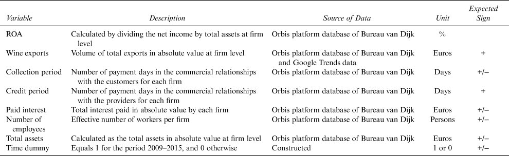
Our dependent variable is return on investment (ROA), reflecting the company's profitability as net income over total assets as a percentage. Lu and Beamish (Reference Lu and Beamish2004) show that ROA is the best way to measure the company's financial performance.
The explanatory variable of interest is wine exports. According to the literature, we expect a positive link between exports and ROA.
We also add a set of control variables, such as collection period and credit period, which capture the quality of payment management regarding commercial relations with customers and providers, respectively. The collection period shows the number of payment days in the commercial relationship with the customers, while the credit period reflects the number of payment days in the commercial relationship with the providers. Tang (Reference Tang2014) suggests that one may expect a positive or negative relation between the collection period and the financial performance of a firm. A higher collection period compresses the operational costs, increases sales, and secures customer loyalty, but, at the same time, it can seriously affect the balance of payment. The credit period is positively connected with financial performances because of lower operational costs. Both variables are expressed in the number of payment days.
An interacted collection-credit period variable is constructed as the ratio between the collection period and the credit period. This is done in order to check for the quality of the management payment period. Given the above assumptions for collection and credit periods, we expect a mixed impact on the financial performance for this interacted variable.
The debt status of a company is measured by interest paid in euros. Its impact on financial performances is controversial. Modigliani and Miller (Reference Modigliani and Miller1958) show a positive influence of debt on profitability, while Smith and Warner (Reference Smith and Warner1979) find a negative one.
Two other variables are alternatively used to test the impact of company size on financial performances: number of employees and total assets. The number of employees captures the number of persons employed in each firm, while total assets are expressed in euros. On the one hand, we can expect a positive correlation between the firm size and the profitability as a result of economies of scale. On the other hand, Mehran (Reference Mehran1995) suggests a negative link as small companies can be more flexible and find better business opportunities.
Finally, a time dummy variable controls for 2015 to 2017, when the relationship between the “Google Trends Wine” index and real country wine exports were weak. It equals 1 for 2009 to 2015 and 0 otherwise.
Except for wine exports, all firm-level variables come from the Orbis platform database of Bureau van Dijk (Reference Bureau van Dijk2018). In order to use the same scale of measurement, all variables used in this paper are normalized and range between 0 and 1.
Detailed information, about the raw variables, for both scenarios, are presented in Tables 1 and 2.
Description of Variables — “Determinants of Exports”

Description of Variables — “Exports and Financial Performances” Analysis

The stationarity property of the normalized variables is tested via the Maddala and Wu (Reference Maddala and Wu1999) test, but only in the second scenario; the variables in the first scenario are generally scalars. We exclusively follow the first generation of the panel unit-root test by assuming cross-sectional independence, the sub-panel being unbalanced (i.e., the second generation of panel unit-root tests assumes cross-sectional dependence and requires balanced panel). Although the panel has a small T compared to N, the unit-root test is employed to simply eliminate any bias doubt, which can influence the quality of estimations.
Finally, variance inflation factors (VIF) test for normalized variables is performed for each scenario in order to detect any multicollinearity issue.
IV. Results and Interpretation
A. Export Determinants
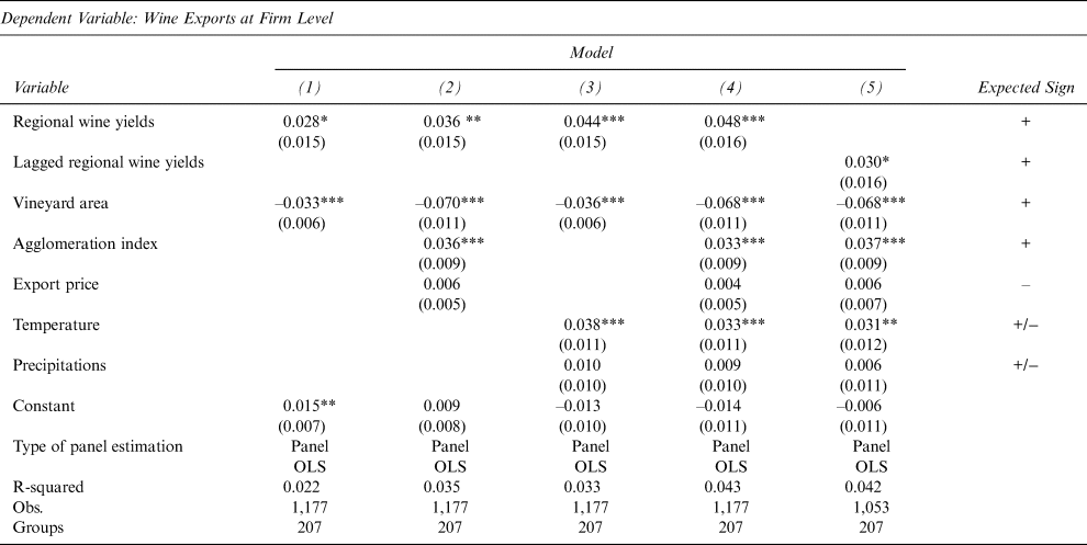
Table 3 reports the results of our export-determinant model drawing on various OLS panel Models (1)–(5).
Empirical Results — “Determinants of Exports” Analysis

Notes: Standard errors in parentheses; statistical significance levels ***(1%), ***(5%), *(10%).
As the VIF average value of 2.48 does not exceed Ringle, Wende, and Becker's (Reference Ringle, Wende and Becker2015) recommended level of 5 or Hair et al.'s (Reference Hair, Anderson, Tatham and Black1995) rule of 10, no evidence of multicollinearity bias is found in our panel models.Footnote 9
Model (1) in Table 3 shows that average regional yields and the vineyard area are key determinants of wine exports in Romania, both are statistically significant. Yields are positively correlated with exports, while the cultivated surface has the opposite impact. Unlike yields, the vineyard area does square with our expectations.
Even when introducing variables capturing specific economic conditions, that is, the agglomeration index and export prices, yields and surface remain significant. The agglomeration index is significant and positively linked with exports; however, the export price is statistically insignificant. The results show that wine producers export more as the concentration of wine companies in an area increases, squaring with the results of Brunow, Pestel, and Partridge (Reference Brunow, Pestel and Partridge2019).
Model (3) includes weather variables in lieu of the “economic condition” variables. However, only the temperature variable is significant, suggesting that exports increase with higher temperatures. This is partially in line with Cahill et al. (Reference Cahill, Lobell, Field, Bonfils and Hayhoe2007).
Finally, Model (4) includes all determinants mentioned earlier, which, with the exception of export price and precipitations, are all significant. Exports are stimulated by higher yields in the wine industry, smaller cultivated surfaces, agglomeration economies, and higher temperatures (i.e., considered as a key element for the wine quality). In Model 5, we use the lag of wine yields. This variable is statistically significant and has a positive sign as in Model (4), suggesting a positive impact of the past year's wine exports. All other variables remain significant and have similar coefficients as in Model (4).
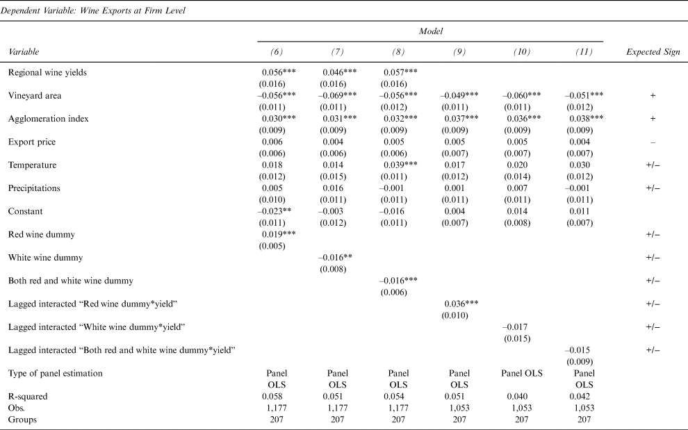
Next step, we analyze the impact of specific wine varieties on exports. Table 4 presents the full OLS Panel Models (4) and (5) extended with wine variety dummies and lagged interacted “variety of wine dummy-wine yields,” respectively.
Empirical Results — “Determinants of Exports” Analysis Considering the Wine Varieties

Notes: Standard errors in parentheses; statistical significance levels ***(1%), ***(5%), *(10%).
The results (Models 6–11) suggest that only the regional specialization in red wine varieties is positively correlated with wine exports, while white varieties, and both red and white ones, are negatively linked to exports. Moreover, Models (9)–(11) show that the lagged interacted “red wine dummy-yields” remains positively correlated with wine exports, while the lagged interacted “both red and white wine dummy - yield” has a negative sign.
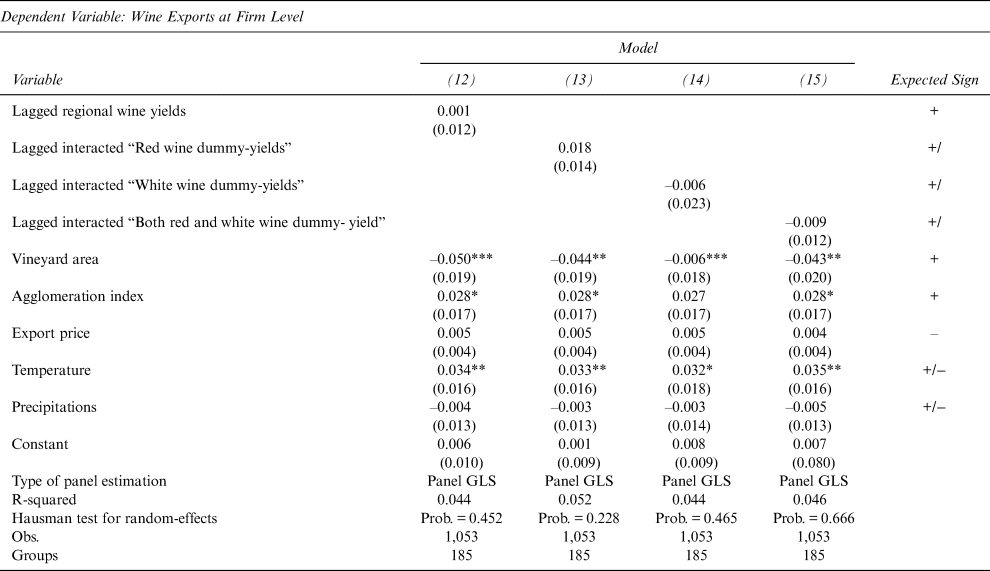
Table 5 shows the unobserved heterogeneity is modeled by using GLS estimators.
Export Determinants Analysis with Random Effects

Notes: Standard errors in parentheses; statistical significance levels ***(1%), ***(5%), *(10%).
The Hausman tests suggest that random-effects are more appropriate than fixed-effects in all scenarios. Models (12)–(15) show that the vineyard area, the agglomeration index, and temperature are still significant in all estimations, maintaining their previous signs. However, we find lagged wine yields (in Model 12) or lagged interacted “variety of wine dummy*yield” (in Models (13)–(15), respectively) to be statistically insignificant, suggesting that wine exports are randomly sensitive to regional conditions.
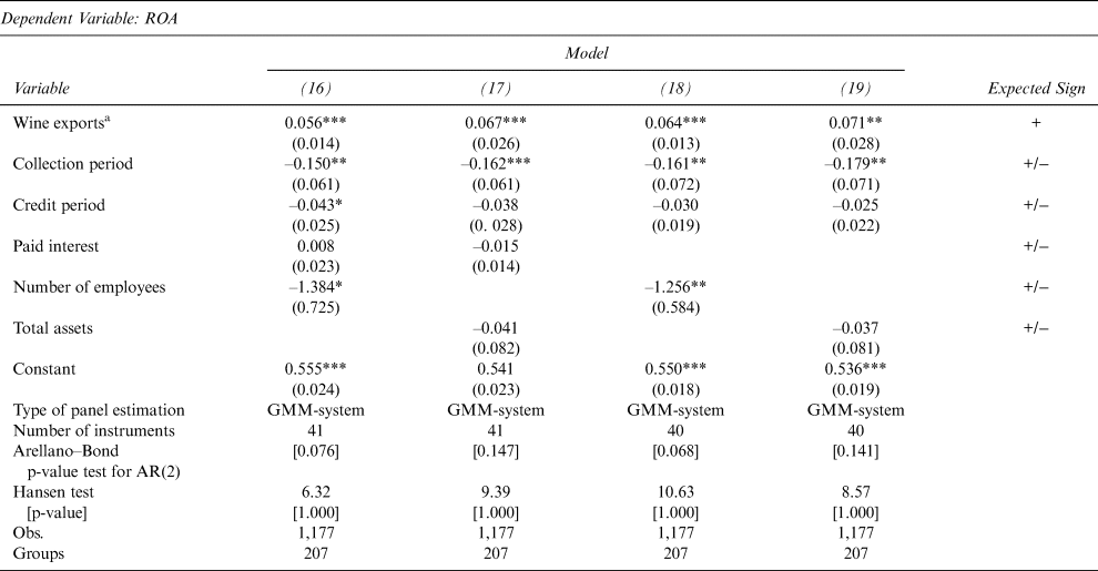
Table 6 reports the results of our GMM-system panel Models (16)–(19).
GMM-System Panel Model Exports and Financial Performance

Notes: Standard errors in parentheses; statistical significance levels ***(1%), ***(5%), *(10%).
a Firm-level wine exports obtained using Google Trends data.
The results of Maddala and Wu's (Reference Maddala and Wu1999) test for panel unit root suggest that all normalized variables used in this step are stationary in level. Moreover, no multicollinearity issue is detected, as the average value of the VIF test (1.30) is lower than the critical level.Footnote 10
The GMM-system estimations deal with the endogeneity generated by the reverse causality of “financial performance - exports” (Melitz, Reference Melitz2003). The main instruments used to fix the issue are two proxies of “wine exports” (i.e., wine yields and vineyard area) and the lagged values of wine exports.
Model (16) suggests that exports have a significantly positive impact on ROA. Both credit and collection period variables are significant but negatively correlated with ROA, while paid interest is insignificant. Controlling for company size using the number of employees, we find that there is a significant and negative correlation between the number of workers and ROA. The negative sign seems to be explained by a lower yield, seen as a consequence of lower employee engagement in the Romanian wine sector (Harter, Schmidt, and Hayes, Reference Harter, Schmidt and Hayes2002); this may be explained by the fact that most of the workers in this sector are seasonal with fixed-term contracts.
Model (17) also controls for the company size, but through the total assets. This variable, however, is not significant. Here, the exports and the collection period maintain their significance and signs as in the previous model, while the credit period and paid interest lose their significance.
Models (18) and (19) alternatively use the number of employees and the total assets, removing the effect of the paid interest. The exports, the collection period, and the number of employees are significant, having the sign put forward in the previous estimations, while the credit period and total assets are not significant.
Overall, the results show that the wine exports variable has a positive impact on ROA in all model versions, which is in line with the findings of Fryges and Wagner (Reference Fryges and Wagner2010). It is also noteworthy that the collection period and the number of employees are robust, both having a negative impact on ROA. These findings are in line with Tang (Reference Tang2014) in terms of the collection period and Mehran (Reference Mehran1995) regarding the company size. Paid interest, credit period, and total assets are not significant in the analyzed scenarios. Moreover, it seems that firm exports are enhanced in regions specializing in red wine.
V. Robustness Check
We run robustness checks at two levels. First, we introduce more variables in the model that explains the relation between financial performances and exports. We include a time period variable to account for changes over the considered period and an interaction between the collection and the credit variables. Second, two alternative variables will be used to capture the wine exports: the wine exports (all) and the wine exports (only significant). These variables are the estimated wine exports, obtained by using two econometric strategies that will be described later in this section.
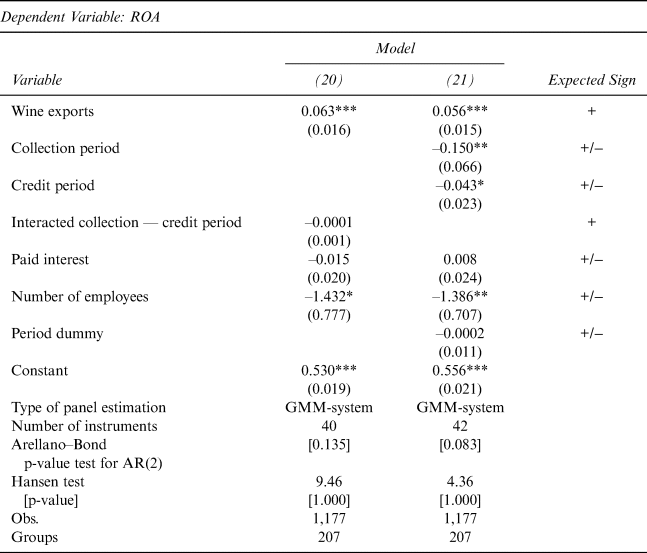
A first robustness check is run for the model that links financial performances and regional-firm-level wine exports (obtained by drawing on Google Trends data). We aim at taking account of the impact that the time dimension of our study can have on the results (in this respect, a time period dummy is used) and of possible interactions between key variables presented in Equation (2). The results are presented in Table 7.
GMM-System Panel Model Exports and Financial Performance — Robustness Check

Notes: Standard errors in parentheses; statistical significance levels ***(1%), ***(5%), *(10%).
Model (20) introduces a new variable capturing the interaction between the collection period and the credit variable in order to check for the quality of the payment management period, using the number of employees as a control for the company size. The variables exports and number of employees are significant, maintaining their previous signs, while the interacted variable is not significant. Finally, Model (21) analyzes the same relation while controlling for the period with a lower correlation between “Google Trends Wine” index and the real country wine exports (“a disconnected period”). The dummy period is insignificant, suggesting that the observed “disconnection” does not generate a bias in estimations. Moreover, wine exports, the collection period, and the number of employees remain significant, keeping the signs they had in previous estimations.
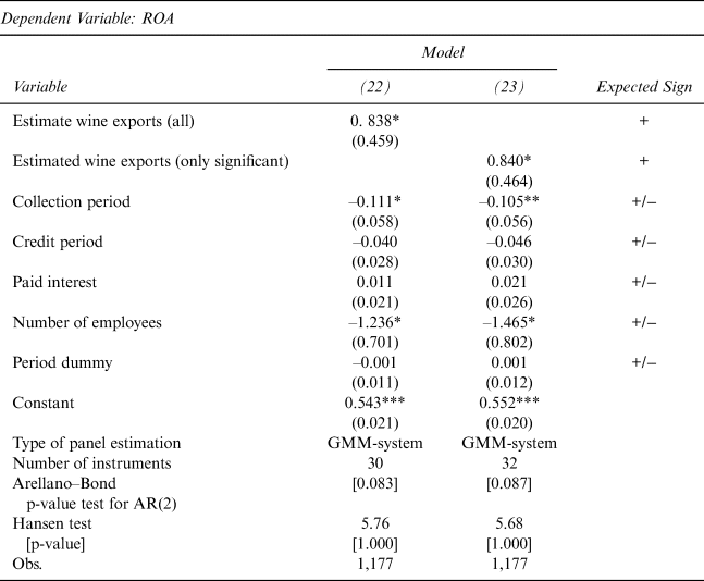
In a second robustness check, we measure the “wine exports” index using estimated wine exports. To do so, we use a two-step approach. First, we run the full Model (12) (Table 5) and obtain estimated wine exports drawing on both significant and non-significant variables in the regression. We call this variable wine exports (all). We then employ the same approach but only include the significant regressors and call this variable wine exports (only significant). We follow this approach in order to avoid any potential bias generated by omitted variables. In a second step, we run Equation (2), which links financial performances and exports, alternatively, with the two estimated wine export variables. The results are presented in Table 8.
GMM-System Panel Model Exports and Financial Performance Robustness Check with Estimated Wine Exports

Notes: Standard errors in parentheses; statistical significance levels ***(1%), ***(5%), *(10%).
These models are run, first, by introducing the time dummy mentioned in Section III, and second, by dropping it from the regressions. As the results do not change (in the presence or in the absence of the time dummy), we present the outcomes obtained in the presence of this variable. They show that both estimated wine export alternatives significantly impact the ROA. The collection period and the number of employees are also significant and have the expected signs.
VI. Conclusion
In the wine industry, exports can play a crucial role in explaining the financial performance of firms. We analyze whether Romanian wine firms could improve their financial performance via exports. Furthermore, we explore the potential drivers of wine exports.
The main results of this study suggest that a high level of exports is associated with better financial performance while controlling for the collection payment period and firm size. In other words, profitability is positively impacted by exports and negatively affected by the collection payment period rise and by additional hired workers. Our results point to higher exports generating more revenue by being able to absorb the associated costs. A reduction of the collection period, without diminishing sales, can then lead to additional cash flows that can further support those operations. The addition of a new employee seems to be related to lower profitability; this might be explained by a lower, work engagement, that is, employees in this sector generally have seasonal jobs with fixed-term contracts. Here, the related costs can be compensated for by higher yields generated by exports, which is one way for companies to achieve economies of scale.
At the same time, the financial performance of Romanian wine producers does not seem influenced by management of the credit payment period or by concomitant adjustment of both “collection” and “credit” payment periods. Finally, we show that Romanian wine exports, at the firm level, are positively associated with higher regional wine yields (especially in the case of red wine varieties) and temperature, as well as with stronger firm agglomeration, and negatively affected by the vineyard size.