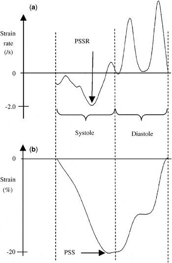


Strain and strain rate are parameters for assessing regional myocardial function in adultsReference Heimdal, Stoylen, Torp and Skjaerpe1–Reference Ingul, Stoylen and Slordahl8 and children,Reference Weidemann, Eyskens and Jamal9 the parameters both measuring deformation. Myocardial strain describes the deformation of a myocardial segment relative to its original length, while the strain rate is the strain per unit of time (Fig. 1).Reference Heimdal, Stoylen, Torp and Skjaerpe1 Analysis of the parameters requires initial recording of the images using tissue Doppler, followed by the analysis itself. Several additional parameters must be set both during acquisition and analysis. Analysis using tissue Doppler is noisy, and the ratio of signal to noise is more unfavourable when assessed in small segments.Reference Heimdal, Stoylen, Torp and Skjaerpe1, Reference D’hooge, Heimdal and Jamal10 It is important, therefore, to choose settings during acquisition and off-line analysis that provide measurements with the lowest possible noise, be the measurements made in adults or neonates. We have already shown that the noise encountered during analysis is dependent on the parameters used for off-line analysis when using images recorded with a 5S phase array probe having a frequency of 2.4 MHz (GE Vingmed, Horten, Norway) and using the default setting for tissue Doppler frame rate.Reference Nestaas, Stoylen, Sandvik, Brunvand and Fugelseth11 If shown to be reproducible, the values obtained using analysis of strain and strain rate could prove useful tools for investigation of myocardial function in neonates.
Example of a curve for strain rate (a) and a curve for strain (b) for one heart cycle. A peak systolic strain rate (PSSR) of −2/s means that the maximal rate of shortening during systole is 2 per second. A peak systolic strain (PSS) of −20% means that the segment has shortened 20% from the end-diastolic length.

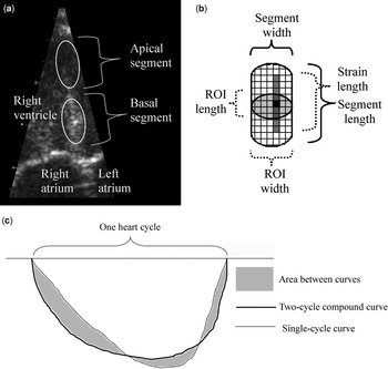
Due to differences in depth and lateral resolution, the settings regarding probe type and tissue Doppler frame rate may provide images with different noises. Further, the impact from the settings chosen for off-line analysis on the noise may be dissimilar when the settings are changed with regard to the type of probe used and the tissue Doppler frame rate. With these possibilities in mind, therefore, we have investigated the impact of different settings during acquisition and analysis on the noise produced when measuring strain and strain rate, hoping to establish the optimal settings for two-segment analyses (Fig. 2).
Basic concepts in analyses of strain and strain rate. The grey scale image (a) of the septum from the apical 4-chamber view shows the area of myocardium used in the apical and basal septal segmental analyses. The relationship is shown between the length and width of the segment, the length and width of the region of interest (ROI), and the strain length (b). The segmental values are estimated by averaging the values for all points within the region of interest (light grey). The values for each point (black square) are estimated by assessing the velocity gradients along the strain length for each point (dark grey). Estimation of the beat-to-beat variation (c). The two cycle compound curve is the curve averaged from two consecutive heart cycles. The beat-to-beat variation is the area between the curves (grey) divided by the area under the compound curve. An example is shown of a strain curve.

Materials and methods
Subjects
We obtained images from 27 healthy term neonates delivered at the Maternity Ward of Ulleval University Hospital. They were examined during the first, second, and third day of life from March to May 2005. Their mean weight at birth was 3.72 kilograms, with a 95 percent confidence interval from 3.53 to 3.90 kg. The mean gestational age was 40.8 weeks, with a 95 percent confidence interval from 40.4 to 41.1 weeks, and the median Apgar score at 5 minutes was 9, with a range from 8 to 10. We obtained written informed parental consent, and the project was approved by the Regional Committee for Medical Research Ethics, and by the scientific committee at Ulleval University Hospital.
Measurements
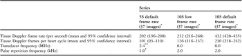
Tissue Doppler images were recorded using the 10S phased array probe (Vivid 7 Dimension v 4.0.1 built 1644, GE Vingmed, Horten, Norway), with a frequency of 8 MHz, and a range of tissue velocities from −0.16 to 0.16 metres per second, corresponding to a pulse repetition frequency of 2.0 kHz (Table 1). The ultrasonic beams were kept parallel to the myocardial wall. We recorded one series of images using the default settings for tissue Doppler frame rate, and another series using a low frame rate. The sector angle was mainly around 30 degrees. During recording, it is necessary to set the degree of averaging between velocities for adjacent points in the radial and lateral direction. The lateral averaging can be adjusted in steps from 0 to 4, and the radial averaging in steps from 0 to 3. The default settings were step 0 of 4 for the lateral averaging, and step 3 of 3 for the radial averaging, and these settings were used in this study.
Details for the tissue Doppler images.

*No difference between each series wall distribution, Chi-square p>0.995 for all pair wise comparisons.
**Transducer frequency was 2.2 MHz in one image.
†Pulse repetition frequency was 0.99 kHz in one image.
We recorded 13 examinations with the default frame rate, and 11 examinations with the low rate. We had planned 2 more examinations at the low rate, but the data was lost in 1 due to a problem with storage, while in another neonate, an asymptomatic left-sided pneumothorax made apical ultrasonic imaging impossible. In all examinations, we studied 9 cardiac walls, as in our previous study.Reference Nestaas, Stoylen, Sandvik, Brunvand and Fugelseth11 We examined the left ventricular lateral wall, the septal wall, and the right ventricular lateral wall from the four-chamber view, the left inferior and anterior wall of the left ventricle using the two-chamber view, the anterior septum and left inferiolateral wall from the apical long-axis view, the right ventricular inferior wall from the inferior two-chamber view, and the right ventricular anterior wall from the anterior two-chamber view. The inferior and anterior two-chamber views of the right ventricle were achieved by tilting the probe from the four-chamber view to centralise the right ventricle, and then rotating the probe counter clockwise or clockwise to produce the required views.
Protocol
Measurements of tissue Doppler derived strain and strain rate are made within mural segments, and are based on the gradients of velocity of the tissues. The values within an individual segment are estimated by averaging the values for all points within a region of interest. The latter values are estimated by assessing the velocity gradient along a length centred in that point and parallel to the ultrasonic beam, known as the strain length. The segment is the area of the myocardium from which the velocities used in the segment analyses are measured. The width of the segment is the same as the width of the region of interest, while the length of the segment is the sum of the length of the strain length and of the region of interest (Fig. 2).
As in our previous study,Reference Nestaas, Stoylen, Sandvik, Brunvand and Fugelseth11 we quantified the noise in the analyses by estimating the beat-to-beat variation in strain and strain rate (Fig. 2). We analyzed these parameters in 2 consecutive cardiac cycles, extracting the curves for each cycle. We then estimated a 2-cycle compound curve by averaging the curves for the two cycles. The variation from beat to beat was then estimated by dividing the area between the curve of the single cycle and the two-cycle compound curve by the area under the curve for the compound cycle. In noisy analyses, the variation between the measurements for the two consecutive cycles will be larger than in those with less noise. This was quantified by the variation from beat to beat, which is the sum of the true variation between the beats and the variation caused by the noise in the analyses.
To minimize distortion due to low quality of images, we selected for analysis only images of good quality from the series obtained using the 10S probe and either the default and low frame rates, judging quality according to visual appearance, finding little or no reverberations or acoustic dropouts in those deemed to be of good quality. We performed 2-segment analyses (Fig. 2) of two consecutive cycles using standard software (Echopac PC SW 4.0, GE Vingmed, Horten, Norway) by measuring the strain and strain rate in the apical and in the basal part of each myocardial wall, using linear drift compensation for the Lagrangian strain curves, and default 40 ms Gaussian smoothing for all analyses. We chose lengths of 1, 3 and 6 mm, and widths of 1, 2, 3 and 4 mm for the region of interest, using strain lengths of 4, 6, 8 and 10 mm, as in our previous study.Reference Nestaas, Stoylen, Sandvik, Brunvand and Fugelseth11 The variation from beat to beat for strain and strain rate were estimated for each of these 48 combinations for all segments. A semi automated tracking system was used to keep the region of interest in the mid segment throughout the cardiac cycle.
In our previous study,Reference Nestaas, Stoylen, Sandvik, Brunvand and Fugelseth11 80 images recorded with the 5S phased array probe had been analyzed in the same way as the images currently obtained using the 10S probe. We selected for comparison, therefore, a similar number of images from that initial study, aiming at a distribution between the walls similar to the images obtained currently for both series using the 10S probe. The ranges of velocity, and averaging settings for the parameters, were equal in all series, with the series obtained using the 5S probe having a pulse repetition frequency of 1.0 kHz (Table 1).
The settings with least random noise will always be the largest combination of the length of the region of interest and strain length. In 2-segment analyses, the length of the segment should then be the half of the length of the wall. The end-systolic lengths of the myocardial walls parallel to the ultrasonic beam were 2.5 cm, or higher. We considered, therefore, a segmental length of from 9 to 12 mm to be appropriate. We then sought the combinations with the lowest noise for each series amongst the settings with the sum of the strain length and the length of the region of interest within this range. The noise was quantified by the variation from beat to beat. Thus, if the variation for one analysis was 10% higher than for another analysis, the noise in the former analysis was regarded as 10% higher than in the latter analysis. The peak systolic strain, and peak systolic strain rate (Fig. 1), were assessed from the 2-cycle compound curves for each series using these settings.
Analysis of data
Chi-square tests were used to test for differences in mural distribution between the series. One-way analysis of variance was used for comparing the beat-to-beat variation for the different settings. Bonferroni correction was used for post hoc pair wise comparisons. A corrected p-value less than 0.05 was considered significant. Combinations with beat-to-beat variation significantly higher than the best found were excluded in stepwise fashion, repeating the procedure until there were no significant differences between the remaining combinations. Values for peak systolic strain and strain rate were compared in similar fashion.
To determine the repeatability of the analyses, one image from each of the walls in the series with the lowest beat-to-beat variation were analyzed 3 times; twice by the same investigator (EN) several weeks apart, and once by another investigator (AS). The intra class correlation coefficients were then assessed for the intra- and interobserver analyses. Using the combination of the size of the region of interest and strain length with the lowest variations, the results obtained were compared using paired sample t-tests.
Results
Data for the tissue Doppler images is shown in Table 1. We obtained 37 images of good quality using the default tissue Doppler frame rate for the 10S probe, and 46 images using the low frame rate as judged by the visual appearance. To obtain an equal number of images in each series, we selected 37 of the 46 images of good quality obtained using the low rate for further analyses. From the 80 images obtained with the 5S probe and analyzed in our previous study,Reference Nestaas, Stoylen, Sandvik, Brunvand and Fugelseth11 we again selected 37 images, choosing a distribution between mural segments similar to those obtained using the 10S probe for both series. In total, we included measurements of 111 images.
Influence of the settings used for acquisition and off line analysis
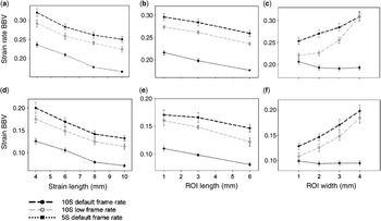
The beat-to-beat variation noted for both strain and strain rate using the 5S probe were lower than the corresponding variation for both series obtained using the 10S probe (p less than 0.05). The beat-to-beat variation using low tissue Doppler frame rates with the 10S probe were lower than when using the default setting for frame rate (p less than 0.05) (Table 2). Each length and width of the region of interest and strain length were associated with significantly lower beat-to-beat variations in strain and strain rate for the 5S probe than the series obtained using the 10S probe (p less than 0.05) (Fig. 3), with values again being lower when using the 10S probe with low frame rates rather than the default setting (p less than 0.05). There were 3 exceptions. When using the 10S probe, we found no significant difference for beat-to-beat variations in strain at a length of 1 mm for the regions of interest, or in beat-to-beat variations for either strain or strain rate at a width of 4 mm for the regions of interest. For each series of measurements, we found that the beat-to-beat variation in both strain and strain rate differed significantly between the strain lengths and the lengths of the region of interest (p less than 0.05), except that no significant difference was found between lengths of the region of interest of 1 and 3 mm when using the default frame rate for the 10S probe and measuring beat-to-beat variation in strain.
Strain and strain rate beat-to-beat variation in each series.

Each value is expressed as mean (95% confidence interval) beat-to-beat variation for the 48 combinations of region-of-interest size and strain length in all segments measured. See text for details.
*Significantly higher than in the 5S series (p less than 0.05).
**Significantly higher than in the 10S low frame rate series (p less than 0.05).
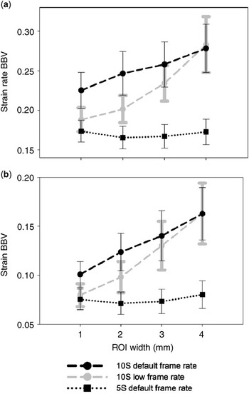
Beat-to-beat variation (BBV) in the strain rate is shown for each strain length (a), length (b) and width (c) of the region of interest (ROI). Beat-to-beat variation is also shown for strain for each strain length (d), length (e) and width (f) of the region of interest. Mean and 95% confidence intervals are depicted. See text for details.

The impact of the width of the region of interest on the beat-to-beat variation in both strain and strain rate was different when using the 5S probe as compared to the 10S probe (Fig 3c, f). There was no significant difference in the values obtained using the 5S probe for different widths of the region of interest, except for a higher variation for strain rate when the width was 1 mm compared to other widths (p less than 0.05). All beat-to-beat variations obtained with the 10S probe were significantly lower when the width of the region of interest was 1 mm compared to all other widths (p less than 0.05), except for no significant difference between widths of 1 and 2 mm in the strain rate analysis in the series obtained using the 10S probe at low frame rate.
Optimal settings for 2-segment analyses
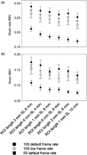
In each of the six combinations with sum of lengths of the region of interest and strain length suitable for 2-segment analyses (Fig. 4), beat-to-beat variations for both strain and strain rate obtained using the 5S probe were significantly lower than the corresponding variation in the series obtained using the 10S probe (p less than 0.05). All variations for strain rate obtained with the 10S probe at low frame rate were lower than the corresponding values obtained using the default frame rate (p less than 0.05). Significant differences for beat-to-beat variation in strain using the 10S probe were found only for two of the six combinations, namely a length of the region of interest of 6 mm and a strain length of 4 mm, and a length of the region of interest of 6 mm and a strain length of 6 mm (p less than 0.05). Beat-to-beat variations for each series were lowest when the length of the region of interest was 1 mm and the strain length 10 mm. Within each series, beat-to-beat variations varied significantly between the combinations (p less than 0.05) but by post hoc tests the beat-to-beat variation within the same series were significantly higher only for a few of the combinations.
Beat-to-beat variations (BBV) in strain rate (a) and strain (b) in all series are shown for all combinations of length of the region of interest (ROI) and strain length (SL) suitable for two segment analysis (segment length 9–12 mm). The cartoon shows mean and 95% confidence intervals.

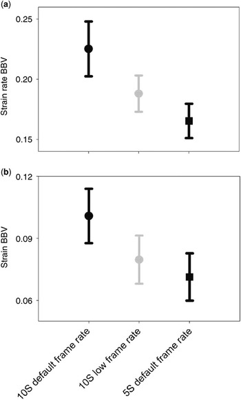
Using a strain length of 10 mm and a length of the region of interest of 1 mm (Fig. 5), we found no significant differences when using the 5S probe for beat-to-beat variations in strain and strain rate between the different widths for the region of interest. All variations using the 10S probe were lowest when the width of the region of interest was either 1 or 2 mm, with no significant differences between these. Beat-to-beat variations for both strain and strain rate were significantly higher using the 10S probe at low frame rates when the width of the region of interest was 3 or 4 mm rather than 1 mm (p less than 0.05). The differences obtained when using the 10S probe at the default frame rate was significant for the strain analyses (p less than 0.05), while the difference for the analyses of strain rate did not reach significance (p equal to 0.054).
Beat-to-beat variations (BBV) for strain rate (a) and strain (b) are shown at each width of the region of interest (ROI) for each series, using a strain length of 10 mm and a length of the region of interest of 1 mm, showing mean values with 95% confidence intervals.

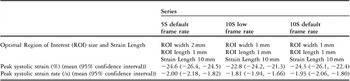
When using the 5S probe, the lowest beat-to-beat variations were found using a strain length of 10 mm, a length of the region of interest of 1 mm, and a width of 2 mm. With the 10S probe, comparable lowest variations were found using a strain length of 10 mm, and length and width of 1 mm for the region of interest. Comparing the variations for all segments in each series using these settings for the analyses, variations were lowest using the 5S probe (Fig. 6). The beat-to-beat variation in strain rate was significantly higher using the 10S probe for both frame rates (p less than 0.05). The beat-to-beat variation in strain was significantly higher using the 10S probe at the default frame rate (p less than 0.05), while the difference between these values and those obtained at low frame rate was not significant. Beat-to-beat variations were significantly higher when using the 10S probe at the default rate compared to the low frame rate (p less than 0.05). Quantified by the beat-to-beat variation for strain and strain rate (Fig. 6), the noise was 13% higher for strain, and 14% higher for strain rate when using the 10S probe at low frame rate compared to the 5S probe. The differences were larger between the probes when the 10S probe was used at the default setting for frame rate, with 42% higher noise for strain, and 36% higher noise for strain rate. There were no significant differences in the two-cycle compound peak systolic strain or peak systolic strain rate between the series when these optimal settings were used (Table 3).
The beat-to-beat variations (BBV) in strain rate (a) and strain (b) are shown for each series, using the optimal strain length and size of the region of interest for two-segmental analysis, showing mean and 95% confidence intervals. The differences between the series were statistically significant (p less than 0.05) except that no differences were found when using the 5S probe and the 10S probe at low frame rates for beat-to-beat variations in strain. See text for details.

Optimal settings and two-cycle compound peak values for two segment strain and strain rate analyses.

Intra- and interobserver measurements
As noise was lowest using the 5S probe, we deemed this series as most appropriate for assessing the intra- and inter-observer analyses, as described in our methodology section. The intraobserver strain beat-to-beat variation intra class correlation coefficient was 0.58 and the intraobserver strain rate beat-to-beat variation intra class correlation coefficient was 0.72. The interobserver strain beat-to-beat variation intra class correlation coefficient was 0.46 and the interobserver strain rate beat-to-beat variation intra class correlation coefficient was 0.49. Of the combinations eligible for two segment analyses, both the strain and the strain rate beat-to-beat variation were lowest using the combination of strain length of 10 mm and length of region of interest of 1 mm in all series analysed. There were no significant differences in beat-to-beat variation recorded for strain or strain rate between the intra- and inter-observer series when using the settings producing the lowest noise.
Discussion
Influence of the settings used for acquisition and off line analysis
The measured variation between two consecutive heart cycles was caused by the true beat-to-beat variation and the noise in the analyses. As the series of images were recorded in the same population, the true beat-to-beat variation was similar, and hence difference in the measured beat-to-beat variation indicated difference in analysis quality between the series. Estimated by the beat-to-beat variation in strain and strain rate, the noise was lower when using the 5S probe, but also lower when using the 10S probe at a low frame rate rather than using the default setting.
The beam transmitted by the 5S probe has a lower ultrasonic frequency than that transmitted by the 10S probe. Such beams of low frequency have deeper penetration. The 5S probe, therefore, is likely to provide more accurate information when depth resolution is needed. High frequency beams have better near-field resolution. The 10S probe, therefore, is more likely to provide more detailed information within the area of penetration. As the noise is lower when using the 5S probe, we suggest that the capability for penetrating the tissue is more important for decreasing the noise in the analyses than the ability for providing detailed near-field information. Hence, use of the 5S probe seems more appropriate when making tissue Doppler recordings in neonates.
The velocities for each point within the myocardium were stored in a velocity grid for each frame during the recording. Velocities for pixels not directly in the path of the ultrasonic beams were estimated by averaging adjacent velocities. The frame rate and beam density were related. Increased frame rate was achieved by reducing the number of beams in each frame, and hence, beam density. With a low beam density, a large amount of interpolated velocities were used. This decreased the lateral resolution, and increased the influence from adjacent beams. The accuracy for each velocity measurement decreased, but as time smoothing was used, the increased frame rate could in part offset this, because each reported value was averaged from more measurements in time. The estimations of strain and strain rate, therefore, were based on more measurements when using the 10S probe at the default rate, while the lateral resolution was higher when using the low frame rate. The lower noise using the low frame rate suggests that higher lateral resolution is more important for providing images with low noise than a high number of velocities in the datasets.
Increasing the strain length reduced noise by improving the ratio of signal, this being the difference between the endpoint velocities, to noise, representing the sum of velocity uncertainties. Increasing the size of the region of interest reduced noise by spatial averaging of more values from a larger area. As we found in our previous study,Reference Nestaas, Stoylen, Sandvik, Brunvand and Fugelseth11 the noise was reduced if the strain length was maintained, even at the expense of the length of the region of interest. When using a long strain length, the estimated velocity gradient proved more accurate, improving the accuracy for each point within the region of interest. Increasing the length increased the area of the region of interest, and hence the number of points from which the regional values were averaged. The measurements were less noisy when increasing the number of velocities used in the gradient estimation than when increasing the number of points for the assessment of regional values.
When using the 5S probe, the noise was similar when the width of the region of interest was 2, 3, or 4 mm. When using the 10S probe, the noise was lowest at the shortest widths. The number of points used in the regional analyses increases in proportion to the area of the region of interest. The regional values were averaged from more points at increasing widths of the region of interest because the area of the region increases in proportion to the width. When increasing the width, the benefit of the increased area due to spatial averaging was countered by lower quality of the signal in the new points. This was especially evident when using higher frame rates, where the lateral resolution was poorest and more of the velocities were interpolated values, but the same effect was also seen at the highest widths when using the 10S probe at low frame rates.
Optimal settings for two-segment analyses
Comparing the combinations suitable for two-segment analyses, the noise in all series was lowest using a length of the region of interest of 1 mm, and strain length of 10 mm. When using the 5S probe, the noise was lowest when the width of the region of interest was 2 mm, whereas the comparable width when using the 10S probe, irrespective of frame rate, was 1 mm. Within each series, the noise was significantly higher only for a few of the other combinations of strain length and size of the region of interest. Using optimal settings, the noise was lowest when using the 5S probe. The differences according to the probe were significant both for measurements of strain and strain rate for the 10S probe at default frame rate, while at low frame rate the differences were significant only for the measurements of strain rate. Quantified by the beat-to-beat variation, the noise was 42% higher for the measurements of strain rate, and 36% higher for the measurements of strain, when using the 10S probe at the default frame rate. They were 14% higher for the measurements of strain rate, and 13% higher for the measurements of strain, when using the 10S probe at low frame rate. These differences may be regarded as clinically relevant. As no differences were found in measurements of peak systolic strain or strain rate between the series, the settings providing the lowest beat-to-beat variation should be used.
Of the settings currently investigated, we suggest that two segment strain and strain rate should be analyzed in images recorded with the 5S probe using the default frame rate. Further, for the off line analyses, a strain length of 10 mm, along with a length of 1 mm and a width of 2 mm should be chosen for the region of interest. If the 10S probe, is used, images should be obtained with a low tissue Doppler frame rate, and analyses should be performed using a width of the region of interest of 1 mm.
Intra- and interobserver measurements
Within the combinations eligible for two-segment analyses, the noise proved lowest for the same combinations of length of the region of interest and strain length in the series analysed between observers, and in both of the series analysed by the same observer, albeit that the intra class correlation coefficients were not very high, probably reflecting the random distribution of noise in the images.
Limitations
The beat-to-beat variation measures the variation between two consecutive heart cycles. Systematic noise is repeated to a greater degree from cycle to cycle, and will not affect the beat-to-beat variation as much as random noise. Thus beat-to-beat variation is not as efficient as a measure of systematic noise. Systematic noise might differ according to the probe and settings of frame rate, and is probably also dependent on other factors, like settings for gain and filters. The impact from these factors has not been investigated. The decreased noise at decreased frame rates was only investigated for the 10S probe, as images with the 5S probe were recorded only using default rates.
Future studies
Assessing the beat-to-beat variation as proposed here might be suitable for comparing other probe and frame rate settings, and noise should be compared using low frame rates with the 5S probe. A more systematic study of the relation between beat-to-beat variation and different kinds of noise should be undertaken, assessing any influence from the quality of the images. Normal values of strain and strain rate in neonates should also be established in a larger series, to assess the impact of the haemodynamic changes on the measurements of contractility. This will give a basis for evaluation of the myocardial performance in neonates with congenitally malformed hearts and circulatory disturbances.
Acknowledgement
Leiv Sandvik advised on the statistical analyses.