



1 Introduction
Approximately half of the observed ice loss from Antarctica and Greenland is due to the calving of icebergs from the margins of the ice sheets (Depoorter et al. Reference Depoorter, Bamber, Griggs, Lenaerts, Ligtenberg, van den Broeke and Moholdt2013; Enderlin & Howat Reference Enderlin and Howat2014). Once the icebergs are calved into the surrounding ocean they are advected by both winds and ocean currents. How rapidly they melt during their drift will determine where the freshwater is released, which has implications for ocean circulation, sea ice formation and biological activity.
Iceberg dynamics and thermodynamics include processes that are still poorly understood. Indeed, there is much interest in comprehending the complex interactions between icebergs and the surrounding ocean, in terms of both how the environment influences the iceberg and vice versa. In particular, the meltwater produced by icebergs has been observed to modify the local ocean physical and chemical properties, affecting both the dynamical response (Helly et al. Reference Helly, Kaufmann, Stephenson and Vernet2011; Stephenson et al. Reference Stephenson, Sprintall, Gille, Vernet, Helly and Kaufmann2015) and the biogeochemical response (Smith et al. Reference Smith, Robison, Helly, Kaufmann, Ruhl, Shaw, Twining and Vernet2007; Duprat, Bigg & Wilton Reference Duprat, Bigg and Wilton2016). Moreover, icebergs are well known to pose a hazard for human activities such as oil platforms, submarine pipelines and, of course, navigation (Bigg & Wilton Reference Bigg and Wilton2014).
Recent numerical works have underlined the importance of correctly describing the iceberg size distribution in order to accurately model sea ice, ocean temperature and ocean salinity (Stern, Adcroft & Sergienko Reference Stern, Adcroft and Sergienko2016; Rackow et al.
Reference Rackow, Wesche, Timmermann, Hellmer, Juricke and Jung2017). The iceberg size distribution is particularly important around Antarctica, where large tabular icebergs with areas that can reach values up to
 $O(10^{3}~\text{km}^{2})$
exist. There, neglecting the giant icebergs can lead to a bias towards the south in the freshwater input, since large icebergs drift further north (Rackow et al.
Reference Rackow, Wesche, Timmermann, Hellmer, Juricke and Jung2017).
Contributions to the melting come from processes acting both above and below sea level. In particular, above the air–sea interface, solar radiation, forced convection due to the winds and sublimation occur, but these processes are generally negligible in terms of the total iceberg decay. At the air–sea interface, wave erosion continuously acts to reduce the iceberg volume both by directly transferring heat from the seawater through the periodic wave motion and by breaking off pieces of the iceberg itself. Below the air–sea interface, buoyant and forced convections significantly contribute to the submarine melting by entraining relatively warmer oceanic water in the turbulent layer attached to the iceberg. Here, buoyant convection refers to the vertical motion associated with the positively buoyant meltwater, while forced convection refers to the relative motion of the water masses, as explained further below. For a comprehensive review of the mechanisms that control iceberg dynamics and melting, the reader is referred to Savage (Reference Savage, Balmforth and Provenzale2001) and Bigg (Reference Bigg2015).
Forced convection is the process that is mainly considered in the present work. In general, it refers to the transfer of heat between a fluid and a body submerged in it through the turbulent boundary layer that develops at the interface due to the relative fluid flow (Eckert & Drake Reference Eckert and Drake1959). In the case of icebergs, the fact that their displacement is controlled by both winds and ocean currents (Wagner, Dell & Eisenman Reference Wagner, Dell and Eisenman2017) provides the relative motion with respect to the ocean. In particular, for large tabular icebergs, even if their displacement is controlled by the ocean currents (Wagner et al. Reference Wagner, Dell and Eisenman2017), there might be relative motion at the base of the iceberg because of the presence of a vertical shear (Bigg Reference Bigg2015; FitzMaurice et al. Reference FitzMaurice, Straneo, Cenedese and Andres2016), because the iceberg is blocked by sea ice or some sea floor topographic features, or because of variations of ocean currents at spatial scales smaller than the iceberg and temporal scales faster than the iceberg response time.
Various efforts have attempted to represent the melting due to the forced convection as a function of the fluid (speed, temperature, salinity) and the ice properties (temperature), to understand better the relevant physical processes and to parametrize the submarine melting in general circulation models (GCMs). The two most widespread parametrizations are those described by Weeks & Campbell (Reference Weeks and Campbell1973) (WC) and Holland & Jenkins (Reference Holland and Jenkins1999) (HJ). They both attempt to model the turbulent flux of heat (and salt) to the ice to calculate the melt rate. WC is built on empirical observations of flow past a heated plate and only considers heat flux (Eckert & Drake Reference Eckert and Drake1959), as described in § 2.1. The HJ parametrization is built upon empirical observations of heat transport in pipe flow (Kader & Yaglom Reference Kader and Yaglom1972) but has been extended to consider both heat and salt transport. Typically, WC is used in studies examining iceberg melting while HJ is used in studies focused on the melting of ice shelves and tidewater glaciers, despite both attempting to model the same heat and salt transport. Since the focus of this work is on iceberg melting, the choice was to model the ice melting with the WC formulation. Examples of the use of the two schemes in GCMs are Bigg et al. (Reference Bigg, Wadley, Stevens and Johnson1997) for the former and Timmermann, Wang & Hellmer (Reference Timmermann, Wang and Hellmer2012) and Rackow et al. (Reference Rackow, Wesche, Timmermann, Hellmer, Juricke and Jung2017) for the latter, amongst others. There is evidence that iceberg melting representation in GCMs is over-simplified, as Stern et al. (Reference Stern, Adcroft, Sergienko and Marques2017) show for tabular icebergs, highlighting that these large icebergs are not currently well represented. Stern et al. (Reference Stern, Adcroft, Sergienko and Marques2017) suggest a newly developed framework in which large icebergs are represented by smaller elements interacting together, which enables the modelling of calving events and iceberg breakup. Active research keeps bringing new insights into how icebergs melt in various dynamical regimes, as in FitzMaurice, Cenedese & Straneo (Reference FitzMaurice, Cenedese and Straneo2017), where an improved version of the WC parametrization is developed to include side melting due to the buoyant meltwater, and in FitzMaurice, Cenedese & Straneo (Reference FitzMaurice, Cenedese and Straneo2018), where the presence of a vertical shear in the flow is shown to significantly alter the submarine melting, compared to a uniform flow case equal to the vertically averaged velocity.
Rotational effects have been shown to be important in the modulation of heat transport in various convective systems. A non-monotonic dependence of the heat transport in Rayleigh–Bénard convection as a function of background rotation is discussed by King et al. (Reference King, Stellmach, Noir, Hansen and Aurnou2009) and King, Stellmach & Buffet (Reference King, Stellmach and Buffet2012). As for horizontal convection, it has been shown that the heat transport generally decreases with increasing rotation (Vreugdenhil, Gayen & Griffiths Reference Vreugdenhil, Gayen and Griffiths2016). Given the importance of heat transport to the melting of icebergs, it is relevant to investigate how rotation can impact ice melting.
The goal of the present study is to quantify the effects of the Earth’s rotation on iceberg melting in a laboratory set-up. For typical values of Antarctic icebergs with length scale
 $L\sim 20$
km, Coriolis parameter
 $f\sim 10^{-4}~\text{s}^{-1}$
and relative flow speed
 $U\sim 10~\text{cm}~\text{s}^{-1}$
(Gladstone, Bigg & Nicholls Reference Gladstone, Bigg and Nicholls2001; FitzMaurice et al.
Reference FitzMaurice, Straneo, Cenedese and Andres2016), the Rossby number
 $Ro=U/fL$
is
 $Ro\sim 0.05$
, which suggests that rotational effects are important. In particular, the possible formation of a Taylor column (TC) under an iceberg and its influence upon melting are explored. The WC parametrization is then extended to try to reproduce the observed variations of the submarine melt rate as a function of the background rotation. In § 2 background information is reviewed. Section 3 describes the experimental methods and set-up, while the results are presented in § 4. Remaining open issues and conclusions are given in § 5.
2 Theoretical background
In the present section, some background information, on which the analysis of the experimental data is based, is reviewed. First, the submarine melt rate parametrization introduced by Weeks & Campbell (Reference Weeks and Campbell1973) is described. It accounts for the relative free stream velocity and is based on the experimental measurements of the heat exchanges of a flow past a flat plate by Eckert & Drake (Reference Eckert and Drake1959). Second, the dynamics leading to the formation of TCs is reviewed. The analytical solutions obtained for this problem by Ingersoll (Reference Ingersoll1969) and Johnson (Reference Johnson1983) are the starting points for the inclusion of rotational effects in the WC parametrization, due to the modifications of the flow structure as the background rotation changes.
2.1 Submarine melting parametrization
Following an experimental procedure similar to the work of FitzMaurice et al. (Reference FitzMaurice, Cenedese and Straneo2017), the focus of this work is on the melting due to forced convection and its representation by the WC parametrization. This parametrization describes the submarine melt rate
 $\dot{v}$
, i.e. the iceberg volume loss per unit area per unit time, as a function of the relative flow speed
 $U$
, the forcing temperature
 $\unicode[STIX]{x0394}T=T_{w}-T_{i}$
(with
 $T_{w}$
denoting the water temperature and
 $T_{i}$
denoting the ice temperature) and the length scale of the iceberg in the direction of the flow
 $\ell$
as
 $$\begin{eqnarray}\dot{v}=K\unicode[STIX]{x0394}T\frac{U^{m}}{\ell ^{1-m}}\quad \text{with}~m=0.8.\end{eqnarray}$$
Here
 $K$
is a constant of proportionality that contains various flow parameters and enables the results from the laboratory to be scaled to the oceans. In particular,
 $$\begin{eqnarray}K=C\frac{kPr^{n}}{\unicode[STIX]{x1D70C}_{i}\unicode[STIX]{x1D6E4}\unicode[STIX]{x1D708}^{m}}\quad \text{with}~C=0.037,\,n=1/3,\end{eqnarray}$$
where
 $\unicode[STIX]{x1D70C}_{i}=917~\text{kg}~\text{m}^{-3}$
is the ice density (IOC, SCOR & IAPSO 2010),
 $\unicode[STIX]{x1D6E4}=3.34\times 10^{5}~\text{J}~\text{kg}^{-1}$
is the ice latent heat of fusion,
 $k$
is the water thermal conductivity,
 $\unicode[STIX]{x1D708}$
its kinematic viscosity and
 $Pr=c_{p}\unicode[STIX]{x1D70C}_{w}\unicode[STIX]{x1D708}/k$
is the Prandtl number, with
 $c_{p}=3991~\text{J}~\text{K}^{-1}~\text{kg}^{-1}$
as the water specific heat (IOC et al.
2010) and
 $\unicode[STIX]{x1D70C}_{w}=1024~\text{kg}~\text{m}^{-3}$
as its density. The values of
 $C$
,
 $n$
and
 $m$
are based on the experimental work of Eckert & Drake (Reference Eckert and Drake1959) on forced convection along a flat plate. These values depend on the geometry of the obstacle, but for the range of parameters explored in the present work the melt rate given by the WC parametrization does not significantly change if the values for a cylindrical obstacle are used (not shown). By choosing the appropriate values for the physical parameters in SI units, given in table 1, one finds
 $K=8.67\times 10^{-6}$
for the laboratory and
 $K=6.27\times 10^{-6}$
for the oceans, so that the results scale accordingly. More details about the derivation of the WC parametrization can be found in Weeks & Campbell (Reference Weeks and Campbell1973) and FitzMaurice et al. (Reference FitzMaurice, Cenedese and Straneo2017).
Values of thermal conductivity and kinematic viscosity used to calculate
 $K$
in the laboratory and in the oceans (FitzMaurice et al.
Reference FitzMaurice, Cenedese and Straneo2017).

It is interesting to notice that, despite salinity having been shown to be important in affecting the melt rate of ice (Kerr & McConnochie Reference Kerr and McConnochie2015), it is not included in the WC parametrization. In the current set-up, this is reasonable because the ice is melting purely due to the fact that the water temperature is much higher than the melting point of ice and, thus, the phase change is controlled by the heat flux alone (Kerr & McConnochie Reference Kerr and McConnochie2015). However, the melting of icebergs in the polar ocean is likely to depend on both the ambient temperature and the salinity.
FitzMaurice et al. (Reference FitzMaurice, Cenedese and Straneo2017) have tested the WC parametrization behaviour for a range of flow speeds. They find that for low flow speed
 $U$
, the buoyant convection due to the meltwater plumes controls the iceberg lateral melt rate. This happens because the meltwater produced by the ice block itself, despite being cooler than the environment, is buoyant due to its lower salinity content and moves upwards forming plumes along the sides of the ice block. For low relative flow velocity,
 $U<w_{p}$
, where
 $w_{p}$
is the typical value of the vertical velocity of the plume (see Wells & Worster (Reference Wells and Worster2008) for a detailed model of the buoyant plume behaviour near the ice surface), the melting is correctly parametrized by WC using the iceberg draft as length scale and the buoyant plume temperature and velocity in (2.1). Instead, for higher velocity,
 $U>w_{p}$
, the WC parametrization with the free stream quantities and the iceberg length fits the data well. In the former regime, the buoyant meltwater plumes remain attached to the ice block, which is thus unaffected by the free stream flow, and in the latter, the plumes are swept away and the free stream velocity and temperature control the forced convection that melts the ice block.
2.2 Taylor column dynamics
Let us now consider a barotropic, inviscid, incompressible, rotating flow, with low Rossby number
 $Ro=U/fL$
, where
 $U$
is the velocity scale,
 $f=2\unicode[STIX]{x1D6FA}$
(the Coriolis parameter) is the background vorticity (
 $\unicode[STIX]{x1D6FA}$
is the background rotation rate) and
 $L$
is the length scale of the flow. Under these conditions, the Taylor–Proudman theorem can be proved (Vallis Reference Vallis2006). In fact, by neglecting the inertial terms in the geostrophic limit (
 $Ro\ll 1$
), and by neglecting the viscous and baroclinic terms for an inviscid incompressible fluid, the vorticity equation states that the fluid velocity
 $\boldsymbol{v}$
is uniform in the direction of the axis of rotation
 $z$
, namely
 $$\begin{eqnarray}\frac{\unicode[STIX]{x2202}\boldsymbol{v}}{\unicode[STIX]{x2202}z}=0\quad \text{for}~Ro\ll 1.\end{eqnarray}$$
This implies that, if an obstacle is placed somewhere in the domain, the flow is forced to go around it not only at the depth where the obstacle is physically present, but also everywhere above (or below) the obstacle. It is as if the obstacle was virtually extended throughout the entire fluid column. This virtual obstacle is stagnant and has been called a TC (Taylor Reference Taylor1923).
The analytical steady-state solution for the velocity field in the case of a cylindrical obstacle is given by Ingersoll (Reference Ingersoll1969) for a uniform background flow and by Johnson (Reference Johnson1983) for a horizontally sheared background flow. They both consider a constant background fluid flow rotating at a constant rate and confined between two horizontal parallel flat plates, distanced
 $H$
from each other and with a cylindrical obstacle of height
 $h<H$
placed on one of the plates. Using a perturbation approach in terms of
 $Ro$
, they find that to the lowest order the interior solution is two-dimensional and geostrophic. Ingersoll (Reference Ingersoll1969) finds that the steady-state solution for the zeroth-order horizontal velocity, denoted with
 $u^{(0)}(x,y)$
in what follows, depends only on the parameter
 $$\begin{eqnarray}\unicode[STIX]{x1D6FC}=\frac{Ro}{h_{0}}=\frac{U}{fL}\frac{H}{h},\end{eqnarray}$$
where
 $h_{0}=h/H$
is the non-dimensional height of the obstacle. Instead, Johnson (Reference Johnson1983) derives a solution that depends on
 $\unicode[STIX]{x1D6FC}$
and on
 $$\begin{eqnarray}\unicode[STIX]{x1D6FD}=\frac{\unicode[STIX]{x0394}U/\unicode[STIX]{x0394}y}{f}\frac{H}{h},\end{eqnarray}$$
where
 $\unicode[STIX]{x0394}U$
is the change in horizontal velocity over a cross-flow distance
 $\unicode[STIX]{x0394}y$
.
From a dynamical point of view, the problem is solved with the appropriate potential vorticity conservation equation. Such a constraint induces an anticyclonic relative vorticity anomaly due to the compression of the water column in response to the obstacle. In the case of horizontally sheared background flow, the solutions differ as to whether the vorticity added by the horizontal shear has the same sign as or opposite sign to that of the vorticity anomaly induced by the fluid being squeezed below the obstacle. For the interested reader, the analytical solution for the case of positive
 $\unicode[STIX]{x1D6FD}$
, which applies to the current set-up, is given by equations (3.5) and (3.11) of the paper by Johnson (Reference Johnson1983). In particular, such equations give the streamfunction over the entire domain (both below the obstacle and outside it), from which the velocity field can be obtained.
The colours indicate the difference between the analytical solution for the flow speed under the cylindrical obstacle
 $u^{(0)}(x,y)$
and the far field velocity
 $\tilde{U} (x,y)$
in the case of no shear,
 $\tilde{U} (x,y)=U=4~\text{cm}~\text{s}^{-1}$
, in (a–c) (Ingersoll Reference Ingersoll1969), and with positive horizontal shear,
 $\tilde{U} (x,y)=U+y\unicode[STIX]{x0394}U/\unicode[STIX]{x0394}y$
with
 $\unicode[STIX]{x0394}U/\unicode[STIX]{x0394}y=0.1~\text{s}^{-1}$
, in (d–f) (Johnson Reference Johnson1983) for different values of
 $\unicode[STIX]{x1D6FC}$
. In all cases
 $h=2$
cm and
 $H=12$
cm. The dotted areas denote negative values of such a speed difference. The green solid thick line is the section of the cylindrical obstacle which has radius
 $L=12.5$
cm. The black solid thin lines are streamlines and for anticlockwise rotation (Northern Hemisphere) the flow goes from left to right, as the relative vorticity anomaly induced by the obstacle is anticyclonic. The closed streamlines within the section of the obstacle in (c,e,f) delimit regions of no motion, i.e. partial TCs.
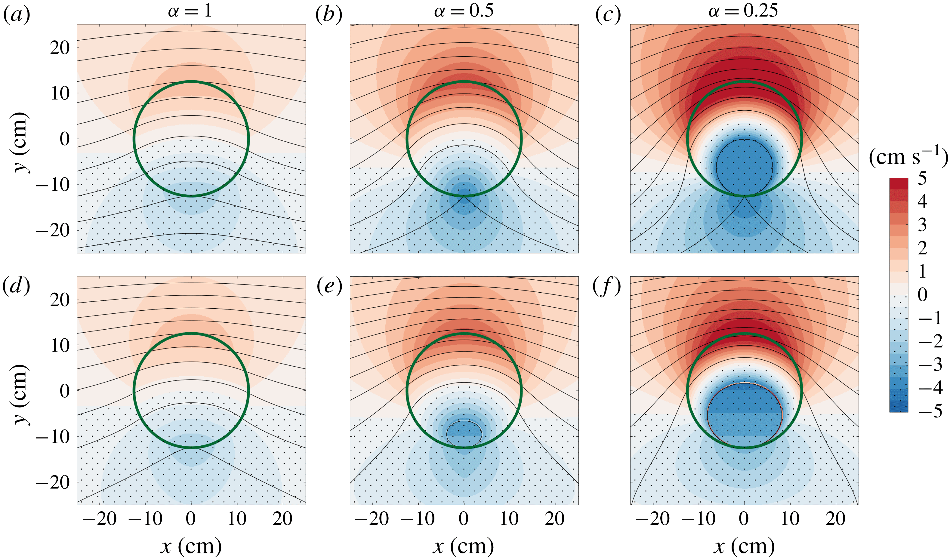
Figure 1 shows the analytical steady solution of the TC problem outlined above, both for zero horizontal shear (figure 1
a–c) and for a positive shear (figure 1
d–f). The parameters used to plot this figure are taken from the experimental set-up, as described in § 3. The top row is obtained for a uniform far field velocity
 $\tilde{U} (x,y)=U$
, with
 $U=4~\text{cm}~\text{s}^{-1}$
, while the bottom row is obtained for a positively sheared flow
 $\tilde{U} (x,y)=U+y\unicode[STIX]{x0394}U/\unicode[STIX]{x0394}y$
, with
 $\unicode[STIX]{x0394}U/\unicode[STIX]{x0394}y=0.1~\text{s}^{-1}$
. The different columns correspond to different values of
 $\unicode[STIX]{x1D6FC}$
and, going from left to right, they show the transition from a no-TC solution to a partial TC one. It is known, in fact, that as
 $\unicode[STIX]{x1D6FC}$
decreases, a stagnation point appears in the velocity field. Huppert (Reference Huppert1975) showed that such a critical value
 $\unicode[STIX]{x1D6FC}_{c}$
depends on the geometry of the obstacle and on the stratification of the fluid. He also showed that for a cylindrical obstacle in a uniform flow of a homogeneous fluid the critical value is
 $\unicode[STIX]{x1D6FC}_{c}=0.5$
. Panels (a,d) have
 $\unicode[STIX]{x1D6FC}=1>\unicode[STIX]{x1D6FC}_{c}$
and do not have any TC, because the background rotation has a rather small effect on the flow and thus the difference between the velocity magnitude of the flow with respect to the far field (denoted with the colour shading) is small. Panels (b,e) have
 $\unicode[STIX]{x1D6FC}=0.5=\unicode[STIX]{x1D6FC}_{c}$
and in the no-shear case, panel (b), the stagnation point at the lower end of the obstacle is visible as a cusp where the bottom streamline intersects with the obstacle. Panel (e) shows that the presence of a positive shear makes it easier to have a region of no motion, because the added background vorticity due to the positive
 $\unicode[STIX]{x1D6FD}$
is of the same sign as the vorticity anomaly induced by the squeezing of the fluid below the obstacle. Panels (c,f) have
 $\unicode[STIX]{x1D6FC}=0.25<\unicode[STIX]{x1D6FC}_{c}$
and they both show a region of zero motion, i.e. a TC, which is larger for lower values of
 $\unicode[STIX]{x1D6FC}$
(Ingersoll Reference Ingersoll1969; Johnson Reference Johnson1983). It is interesting to notice that while on one side of the obstacle a region of zero motion appears, on the other side there is a relative increase in velocity with respect to the far field.
To have a sense of the importance of such dynamics in real oceans, the following typical values of the quantities defining
 $\unicode[STIX]{x1D6FC}$
are considered. Take the relative speed to be
 $U\sim 10~\text{cm}~\text{s}^{-1}$
, the Coriolis parameter
 $f\sim 10^{-4}~\text{s}^{-1}$
, the horizontal length scale of the iceberg
 $L\sim 20$
km, the depth of the water
 $H\sim 10^{3}$
m and the draft of the iceberg
 $h\sim 500$
m. This leads to
 $$\begin{eqnarray}\unicode[STIX]{x1D6FC}=\frac{U}{fL}\frac{H}{h}\sim 0.1,\end{eqnarray}$$
which is below the critical value
 $\unicode[STIX]{x1D6FC}_{c}=0.5$
considered above. This motivates the current investigation because it shows that a TC could form below a sufficiently large iceberg and, thus, could impact its melting. In fact, as shown in figure 1, in the case of formation of a partial TC, a region of increased velocity and a region of decreased velocity appear at the base of the obstacle. Then, since the melt rate depends on the relative speed, as in (2.1), the formation of a TC could increase or decrease the melt rate, depending upon the horizontal extent of the column relative to the area of the object.
3 Experiments
The experiments were conducted in a rotating tank with a diameter of 210 cm, filled to a depth
 $H\simeq 12$
cm with seawater with salinity of approximately
 $33~\text{g}~\text{kg}^{-1}$
and kept at room temperature of 18–
 $20\,^{\circ }\text{C}$
. At least 30 min before the beginning of each experiment, the rotating tank was turned on to set the fluid in solid body rotation with angular velocity
 $\unicode[STIX]{x1D6FA}_{0}$
and corresponding absolute vorticity
 $f_{0}=2\unicode[STIX]{x1D6FA}_{0}$
. The spin-up time that characterizes this transient fluid acceleration has been extensively studied in the past (Greenspan & Howard Reference Greenspan and Howard1963) and is given by the expression
 $$\begin{eqnarray}\unicode[STIX]{x1D70F}_{E}=\frac{H}{(2\unicode[STIX]{x1D708}f_{0})^{1/2}}.\end{eqnarray}$$
For the experimental parameters of this work, the e-folding time varied from roughly 50 s, corresponding to
 $f_{0}=3~\text{rad}~\text{s}^{-1}$
, to 190 s, corresponding to
 $f_{0}=0.2~\text{rad}~\text{s}^{-1}$
, which is much shorter than the time over which the tank was allowed to reach solid body rotation.
Top (a) and side (b) view schematic of the experimental apparatus (not to scale). The presence of horizontal shear is highlighted in (a) by the radially increasing velocity profile
 $\tilde{U} =\tilde{U} (r)=r\unicode[STIX]{x0394}\unicode[STIX]{x1D6FA}$
. The dashed line in (b) underlines that the free surface is parabolic, according to (3.6).
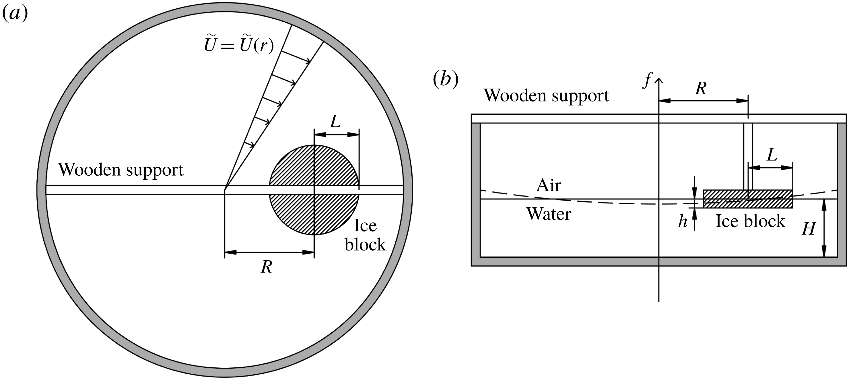
Once the fluid was in solid body rotation, which was confirmed by the vertical straight lines left behind when potassium permanganate crystals were dropped into the fluid, a cylindrical ice block of radius
 $L$
was suspended in the water with a wooden support at a distance
 $R$
from the axis of rotation and with a submerged part of height
 $h$
(see figure 2). As soon as the ice block was in position, the rotation rate of the tank was increased by an amount
 $\unicode[STIX]{x0394}\unicode[STIX]{x1D6FA}$
. This set a relative velocity field
 $\tilde{u}$
between the ice block and the fluid characterized by the radial distance
 $r$
from the centre of the tank and a quasi-exponential decay (Greenspan & Howard Reference Greenspan and Howard1963), namely
 $$\begin{eqnarray}\tilde{u} (r,t)=\tilde{U} (r)\exp (-t/\unicode[STIX]{x1D70F}_{E}),\end{eqnarray}$$
with
 $\tilde{U} (r)=r\unicode[STIX]{x0394}\unicode[STIX]{x1D6FA}$
being the initial velocity profile whose value at the centre of the obstacle is set to be equal to the free stream velocity
 $U$
, namely
 $\tilde{U} (R)=R\unicode[STIX]{x0394}\unicode[STIX]{x1D6FA}=U$
. To keep the relative flow speed almost constant throughout the duration of the experiments, the rotation rate of the tank was further increased by a smaller amount
 $\unicode[STIX]{x1D6FF}\unicode[STIX]{x1D6FA}<\unicode[STIX]{x0394}\unicode[STIX]{x1D6FA}$
at regular intervals
 $\unicode[STIX]{x1D6FF}t$
. In particular, using the equivalent of (3.2) for the angular velocity together with the expression of the spin-up time (3.1), the interval
 $\unicode[STIX]{x1D6FF}t$
at which the tank needs to be accelerated to balance the relative velocity decay is given by
 $$\begin{eqnarray}\unicode[STIX]{x1D6FF}t=-\unicode[STIX]{x1D70F}_{E}\log \left(1-\frac{\unicode[STIX]{x1D6FF}\unicode[STIX]{x1D6FA}}{\unicode[STIX]{x0394}\unicode[STIX]{x1D6FA}}\right),\end{eqnarray}$$
after choosing
 $\unicode[STIX]{x1D6FF}\unicode[STIX]{x1D6FA}$
to be some fraction of
 $\unicode[STIX]{x0394}\unicode[STIX]{x1D6FA}$
. The choice for the experiments was
 $\unicode[STIX]{x1D6FF}\unicode[STIX]{x1D6FA}=\unicode[STIX]{x0394}\unicode[STIX]{x1D6FA}/10$
, so that the values of
 $\unicode[STIX]{x1D6FF}t$
were between 15 and 40 s, depending on the initial background rotation. Since the experiments lasted for 3 min, the number of rotation increase steps was always lower than 12. This procedure was tested for different values of
 $f_{0}$
,
 $R$
and
 $\unicode[STIX]{x0394}\unicode[STIX]{x1D6FA}$
by measuring the fluid angular velocity with floating tracers and it was possible to keep the relative flow speed constant, with fluctuations of the order of 5 % (not shown). The value of background vorticity
 $f$
used to calculate
 $Ro$
and
 $\unicode[STIX]{x1D6FC}$
was taken to be the average between the initial value
 $f_{0}$
and the final one.
The radial increase of
 $\tilde{U} (r)$
also sets its cross-flow derivative, which corresponds to the value of the horizontal shear that appears in the problem solved by Johnson (Reference Johnson1983), namely
 $$\begin{eqnarray}\frac{\unicode[STIX]{x0394}U}{\unicode[STIX]{x0394}y}=\frac{\text{d}\tilde{U} }{\text{d}r}=\unicode[STIX]{x0394}\unicode[STIX]{x1D6FA}.\end{eqnarray}$$
Since
 $\unicode[STIX]{x0394}\unicode[STIX]{x1D6FA}$
is constant for a given value of
 $U$
, this implies that
 $\unicode[STIX]{x1D6FD}$
is directly proportional to
 $\unicode[STIX]{x1D6FC}$
according to
 $$\begin{eqnarray}\unicode[STIX]{x1D6FD}=\frac{L}{U}\frac{\unicode[STIX]{x0394}U}{\unicode[STIX]{x0394}y}\unicode[STIX]{x1D6FC}=\frac{L}{U}\unicode[STIX]{x0394}\unicode[STIX]{x1D6FA}\unicode[STIX]{x1D6FC}.\end{eqnarray}$$
This was chosen so that a single parameter controlled the dynamics, even in the case of horizontally sheared flow. The parameter
 $\unicode[STIX]{x1D6FD}$
could have been varied independently from
 $\unicode[STIX]{x1D6FC}$
, but the study of the dependence of the solution on
 $\unicode[STIX]{x1D6FD}$
is left for future work.
The ice blocks were made in stainless steel cylindrical moulds with radius
 $L=12.5$
cm and height 5 cm, so that they could be half-submerged during the experiments, resulting in values of
 $h\simeq 2$
or 3 cm. The water used to make the ice blocks was degassed and dyed with 2 ml of blue food dye in order to be able to distinguish the meltwater from the ambient fluid in the tank. There are two reasons why the ice blocks were cylindrical. The first is because the focus of this work was on the basal iceberg melting rather than the lateral one. Thus, since the circle is the figure that maximizes the area for a given perimeter, the cylinder has the highest basal to lateral area ratio for a given height. This means that it is the optimal choice to study the melting coming from the base and for the values of the experiments,
 $h\sim 2$
cm and
 $L=12.5$
cm, the area of the base
 $\unicode[STIX]{x03C0}L^{2}$
is roughly three times larger than the area of the side
 $2\unicode[STIX]{x03C0}Lh$
. The second reason is because the analytical solutions for the TC problem, described in § 2.2, have been developed only for flat-topped cylindrical obstacles (Ingersoll Reference Ingersoll1969; Johnson Reference Johnson1983).
The actual fluid height
 $\unicode[STIX]{x1D702}$
varied radially due to the parabolic free surface as
 $$\begin{eqnarray}\unicode[STIX]{x1D702}(r,\unicode[STIX]{x1D6FA})=H+\frac{\unicode[STIX]{x1D6FA}^{2}}{4g}(2r^{2}-D^{2}),\end{eqnarray}$$
with
 $g$
being the acceleration due to gravity,
 $D=105$
cm the radius of the rotating tank and
 $H=12$
cm the non-rotating fluid height. With respect to the flat free surface of the non-rotating case, the deviation on each side of the ice block was approximately
 $$\begin{eqnarray}\unicode[STIX]{x0394}\unicode[STIX]{x1D702}=\unicode[STIX]{x1D702}(R+L,\unicode[STIX]{x1D6FA})-\unicode[STIX]{x1D702}(R,\unicode[STIX]{x1D6FA})\simeq \unicode[STIX]{x1D702}(R,\unicode[STIX]{x1D6FA})-\unicode[STIX]{x1D702}(R-L,\unicode[STIX]{x1D6FA})\simeq 0.8~\text{cm}\end{eqnarray}$$
in the cases of highest rotation rate,
 $f=3~\text{rad}~\text{s}^{-1}$
. All the experiments, even those with the most tilted free surface, were conducted making sure that the upper side of the ice block was never submerged, in order to avoid the introduction of an extra melting source. When calculating the TC dynamics, the water column height at the centre of the ice block
 $\unicode[STIX]{x1D702}(R,\unicode[STIX]{x1D6FA})$
was used.
For each experiment, two quantities were measured: the mass loss
 $\unicode[STIX]{x0394}m$
and the initial submerged draft
 $h$
. The mass loss was measured by weighing the ice block before and after each experiment and was converted to a volume loss
 $\unicode[STIX]{x0394}V=\unicode[STIX]{x0394}m/\unicode[STIX]{x1D70C}_{i}$
from the known density of the ice
 $\unicode[STIX]{x1D70C}_{i}=917~\text{kg}~\text{m}^{-3}$
(IOC et al.
2010). The initial submerged draft was measured with a ruler as the difference between the initial height of the ice block (measured before the experiment) and the height of the non-submerged part (measured right after the experiment). The melting of the non-submerged part of the blocks was observed to be negligible. For each block, to remove the asymmetry due to the free surface tilting, the measure was taken in four antipodal points and then averaged. Then
 $\dot{v}$
was calculated assuming the melt rate to be equal on the base and on the sides (this assumption is discussed in more detail at the end of § 4) and uniform for the duration of an experiment,
 $\unicode[STIX]{x0394}t=3$
min. The duration of the experiments was chosen as a compromise. A shorter time interval would have reduced the asymmetries in the ice block melting, due to the presence of horizontal shear in the flow and due to the free surface tilting. A longer time interval would have allowed more ice to melt, inducing a larger mass loss and thus reducing its relative uncertainty.
With these hypotheses, the submarine melt rate was calculated as
 $$\begin{eqnarray}\dot{v}=\frac{\unicode[STIX]{x0394}V}{A_{a}\unicode[STIX]{x0394}t},\end{eqnarray}$$
where
 $A_{a}$
is the average submerged area between the initial state and the final one. Since the melt rate is considered constant and uniform, the average area
 $A_{a}$
is the arithmetic mean between the initial submerged area
 $A_{i}=\unicode[STIX]{x03C0}(L^{2}+2Lh)$
and the final one
 $A_{f}$
. The latter is obtained considering that each dimension is reduced by a length equal to the product of the melt rate and the duration of the melting,
 $\dot{v}\unicode[STIX]{x0394}t$
, namely
 $A_{f}=\unicode[STIX]{x03C0}[(L-\dot{v}\unicode[STIX]{x0394}t)^{2}+2(L-\dot{v}\unicode[STIX]{x0394}t)(h-\dot{v}\unicode[STIX]{x0394}t)]$
. Explicitly, the average area is
 $$\begin{eqnarray}A_{a}=\frac{\unicode[STIX]{x03C0}}{2}[L^{2}+2Lh+(L-\dot{v}\unicode[STIX]{x0394}t)^{2}+2(L-\dot{v}\unicode[STIX]{x0394}t)(h-\dot{v}\unicode[STIX]{x0394}t)],\end{eqnarray}$$
which is equivalent to the assumption that the measured mass loss constrains the value of the final area. Equations (3.8) and (3.9) are then solved together for the two unknowns
 $\dot{v}$
and
 $A_{a}$
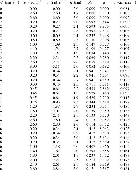
. The parameters and measured quantities for each experiment are given in table 2.
Summary of all the experiments. Parameter
 $U$
is the free stream velocity obtained as
 $U=R\unicode[STIX]{x0394}\unicode[STIX]{x1D6FA}$
. In particular, the ice block is placed at
 $R=[40,40,60]$
cm from the centre of the tank with
 $\unicode[STIX]{x0394}\unicode[STIX]{x1D6FA}=[0.05,0.1,0.1]~\text{rad}~\text{s}^{-1}$
for
 $U=[2,4,6]~\text{cm}~\text{s}^{-1}$
, respectively. Parameter
 $f$
is the average between the initial
 $f_{0}$
and the final value of the background vorticity.
4 Results
In this section, the experimental data obtained from four series of experiments with different values of the free stream velocity,
 $U\in [0,2,4,6]~\text{cm}~\text{s}^{-1}$
, are described. For each value of
 $U$
, a range of values of
 $\unicode[STIX]{x1D6FC}$
was explored by changing the background rotation of the tank, as shown in table 2.
The experimental measurements of the submarine melt rate for all the experiments are shown in figure 3 as a function of the free stream velocity
 $U$
. The data points are colour-coded with the value of
 $\unicode[STIX]{x1D6FC}=Ro/h_{0}$
, which controls the TC dynamics as described in § 2.2. The orange solid line shows the WC parametrization, as in (2.1), with
 $\unicode[STIX]{x0394}T=18\,^{\circ }\text{C}$
and
 $\ell =2L=25$
cm. The value of
 $K$
, as discussed in § 2.1, contains several physical constants of the system. Here, the laboratory value of
 $K$
is chosen and it is rescaled so that all the inputs of the parametrization are taken in SI units and
 $\dot{v}$
is measured in
 $\text{cm}~\text{min}^{-1}$
. The value of
 $\unicode[STIX]{x0394}T$
is taken to be the difference between the ambient fluid temperature,
 $18\,^{\circ }\text{C}$
, and the melting point of the ice block,
 $0\,^{\circ }\text{C}$
. Despite being in a salty environment, the ice block melts at
 $0\,^{\circ }\text{C}$
because the temperature gradient between ice and water is much larger than the salinity gradient, and thus the ice is in a condition of pure melting with no dissolution. Physically, it means that a thin layer of freshwater insulates the ice block from the seawater, so that the salinity at the interface is zero and the freezing temperature is
 $0\,^{\circ }\text{C}$
, accordingly (Kerr & McConnochie Reference Kerr and McConnochie2015). The length scale of the obstacle to be used in the parametrization is the diameter.
The experimental uncertainty is
 $\pm 0.01~\text{cm}~\text{min}^{-1}$
based on some repeated experiments. The fact that for
 $U=0~\text{cm}~\text{s}^{-1}$
and
 $U=2~\text{cm}~\text{s}^{-1}$
the measured melt rate is significantly higher than the parametrized one is indicative of the action of another process controlling the melting for low free stream velocity, similar to what was found for the side melt rate by FitzMaurice et al. (Reference FitzMaurice, Cenedese and Straneo2017). The hypothesis is that at low
 $U$
, the positively buoyant meltwater formed at the base of the ice block flows as a gravity current which moves faster than the free stream velocity. Unfortunately, due to the experimental tank having opaque walls, it was not possible to accurately observe this process at the base of the ice block. Thus, further experiments with submerged cameras and/or in a non-rotating transparent tank are encouraged to better observe and understand what happens at the base of the ice block for low
 $U$
.
To include the effect of this basal meltwater gravity current in the submarine melt rate dependence on the free stream velocity, a constant
 $\dot{v}$
below a certain threshold velocity
 $U_{t}$
is introduced (shown as a black dashed line in figure 3). In particular,
 $U_{t}$
is calculated from the WC parametrization as
 $$\begin{eqnarray}U_{t}=\left(\frac{\dot{v}_{U=0}\ell ^{0.2}}{K\unicode[STIX]{x0394}T}\right)^{5/4},\end{eqnarray}$$
imposing the melt rate to be equal to the value obtained from the experiments at zero relative flow velocity, with
 $\dot{v}_{U=0}=0.09\pm 0.01~\text{cm}~\text{min}^{-1}$
. The threshold value is
 $U_{t}=3.8\pm 0.5~\text{cm}~\text{s}^{-1}$
. Data points at high
 $\unicode[STIX]{x1D6FC}$
(low relative rotation rate) of both the
 $4~\text{cm}~\text{s}^{-1}$
and
 $2~\text{cm}~\text{s}^{-1}$
series agree quite well with this constant value (figure 3).
Submarine melt rate as a function of the free stream velocity
 $U$
. The experimental uncertainty is shown in the upper left corner of the figure. The WC parametrization, (2.1), is shown as an orange solid line. The colour of the data points is chosen according to the value of
 $\unicode[STIX]{x1D6FC}$
of each experiment. A constant
 $\dot{v}$
line is added (black dashed) corresponding to the experimental value obtained with no relative flow,
 $\dot{v}_{U=0}=0.09~\text{cm}~\text{min}^{-1}$
, for a free stream velocity below the threshold
 $U_{t}=3.8~\text{cm}~\text{s}^{-1}$
. See the text for further details.

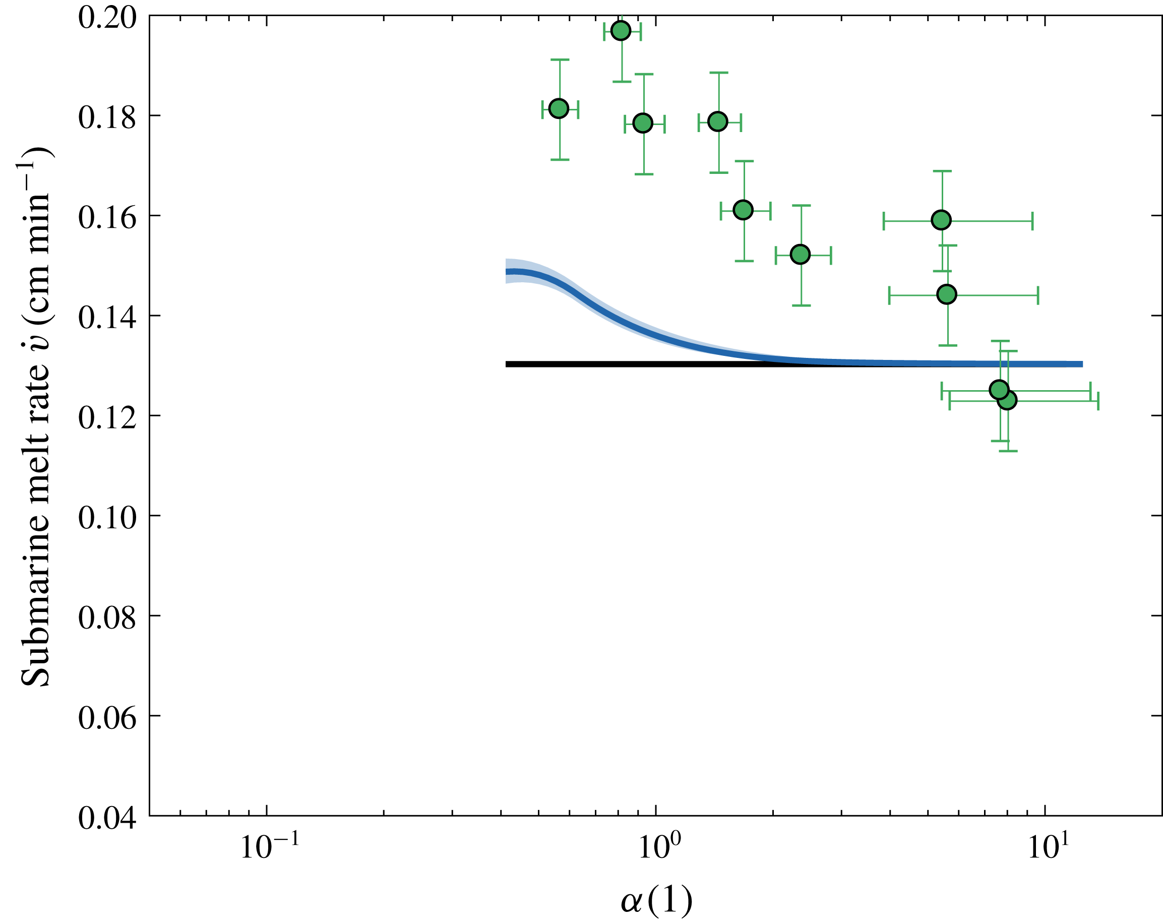
Considering, now, the series of experiments with approximately constant non-zero free stream velocity, the experimental submarine melt rate generally increases as
 $\unicode[STIX]{x1D6FC}$
decreases. The melt rate as a function of
 $\unicode[STIX]{x1D6FC}$
for
 $U=[2,4,6]~\text{cm}~\text{s}^{-1}$
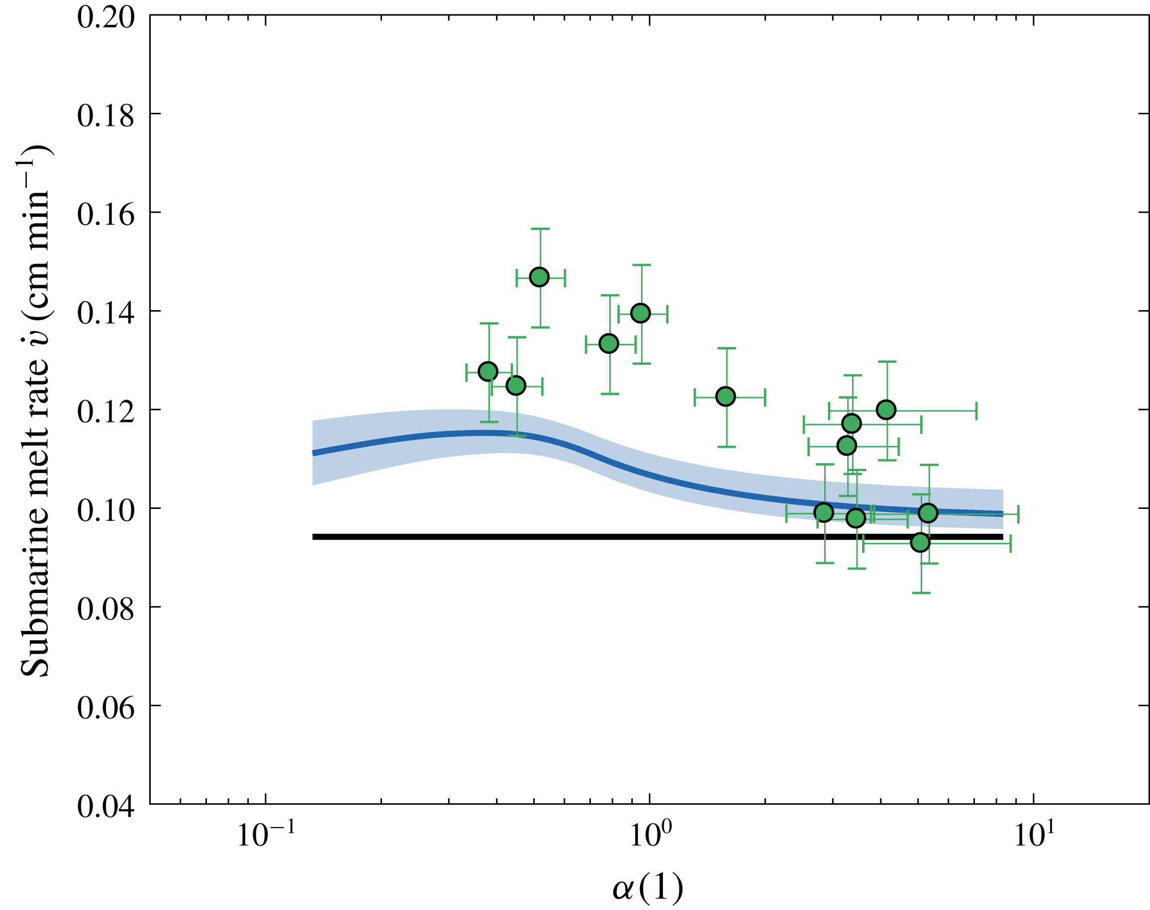
is shown in figures 4, 5 and 6, respectively. The data points, together with their uncertainty, are shown as green circles. The uncertainty on
 $\unicode[STIX]{x1D6FC}$
comes both from the experimental uncertainty on
 $h$
, the draft of the ice block, and from the fact that to maintain the relative velocity
 $U$
constant, the rate of rotation had to increase throughout the experiment, as explained in § 3. The black solid line denotes the value of the WC parametrization calculated for the specified
 $U$
. The parametrized melt rate is constant because it does not depend on the background rotation rate.
To include the effect of the TC dynamics on the melting of the iceberg, an effective velocity
 $u^{\ast }(r,\unicode[STIX]{x1D703})$
, where
 $\{r,\unicode[STIX]{x1D703}\}$
now denote the set of polar coordinates centred on the obstacle, was calculated. The analytical solution for the velocity field obtained by Johnson (Reference Johnson1983)
 $u^{(0)}(r,\unicode[STIX]{x1D703})$
, introduced in § 2.2 and shown in figure 1, was calculated with the parameters of the experimental set-up for every point under the ice block. Where the velocity was lower than the threshold value calculated in (4.1), it was replaced by
 $U_{t}$
itself, to account for the gravity current dynamics described above. The effective velocity field at the base of the obstacle was written as
 $$\begin{eqnarray}u^{\ast }(r,\unicode[STIX]{x1D703})=\left\{\begin{array}{@{}ll@{}}U_{t} & \text{if}~u^{(0)}(r,\unicode[STIX]{x1D703})<U_{t}\\ u^{(0)}(r,\unicode[STIX]{x1D703}) & \text{otherwise}.\end{array}\right.\end{eqnarray}$$
Then the WC parametrization was calculated with the area-averaged velocity over the base of the cylindrical obstacle, namely
 $$\begin{eqnarray}\overline{U}=\frac{1}{\unicode[STIX]{x03C0}L^{2}}\int _{0}^{2\unicode[STIX]{x03C0}}\text{d}\unicode[STIX]{x1D703}\int _{0}^{L}\text{d}r\,u^{\ast }(r,\unicode[STIX]{x1D703}),\end{eqnarray}$$
instead of the free stream value
 $U$
. The area-averaged velocity was used in the WC parametrization because in their derivation Weeks & Campbell (Reference Weeks and Campbell1973) used a spatial average of the velocity field. Alternatively, one could think of dividing the base of the ice block into smaller regions, according to the value of
 $u^{\ast }(r,\unicode[STIX]{x1D703})$
, and finding the melt rate as an area average of the local melt rate using
 $u^{\ast }(r,\unicode[STIX]{x1D703})$
in the WC parametrization, instead of
 $U$
. But since the dependence of the melt rate
 $\dot{v}$
on the velocity
 $U$
is slightly sublinear,
 $\dot{v}\propto U^{0.8}$
, it was confirmed that calculating the melt rate pointwise using
 $u^{\ast }(r,\unicode[STIX]{x1D703})$
and then averaging over the base of the obstacle did not significantly change the results (not shown). In figures 4–6, the effect of using
 $\overline{U}$
instead of
 $U$
in the calculation of the melt rate using the WC parametrization is shown by the blue line, together with the uncertainty associated with
 $U_{t}$
. This new prediction still underestimates the experimental data, but captures the increasing trend as
 $\unicode[STIX]{x1D6FC}$
decreases.
For
 $U=2~\text{cm}~\text{s}^{-1}$
(figure 4), the velocity is always below the threshold
 $U_{t}$
and thus there is not a strong dependence on the rotation rate, i.e. on
 $\unicode[STIX]{x1D6FC}$
, either in the experimental data points or in the corrected velocity
 $\overline{U}$
WC parametrization, which agree quite well.
For
 $U=4~\text{cm}~\text{s}^{-1}$
(figure 5), the significant increasing trend in the experimental data as
 $\unicode[STIX]{x1D6FC}$
decreases, i.e. the background rotation increases, is visible. For very low
 $\unicode[STIX]{x1D6FC}$
(high background rotation), a decrease in melt rate
 $\dot{v}$
is also visible. This is consistent with the hypothesis that as the area of the TC expands, the region of increased velocity is pushed out of the bottom of the ice block. It was not possible to investigate the behaviour of this decreasing trend for even lower
 $\unicode[STIX]{x1D6FC}$
because the tank rotation became too fast for the ice block to be removed safely and the free surface deviation too large.
For
 $U=6~\text{cm}~\text{s}^{-1}$
(figure 6), even if the
 $\overline{U}$
WC parametrization is further below the data with respect to the
 $U=4~\text{cm}~\text{s}^{-1}$
case, the increase of the melt rate as a function of
 $\unicode[STIX]{x1D6FC}$
is stronger both in the data and in the curve. Thus, the combination of TC dynamics and the threshold behaviour due to the meltwater gravity current observed for low free stream velocity appears to correctly capture the trend of the melt rate as a function of
 $\unicode[STIX]{x1D6FC}$
for all the free stream velocities considered.
Submarine melt rate as a function of
 $\unicode[STIX]{x1D6FC}$
for
 $U=2~\text{cm}~\text{s}^{-1}$
. The black constant line is the WC parametrization calculated with
 $U$
and the blue line, with the shaded area denoting its uncertainty, is the WC parametrization calculated with
 $\overline{U}$
, i.e. it includes both the TC dynamics and the threshold behaviour, as explained in the text.

As in figure 4 but for
 $U=4~\text{cm}~\text{s}^{-1}$
.
As in figure 4 but for
 $U=6~\text{cm}~\text{s}^{-1}$
.
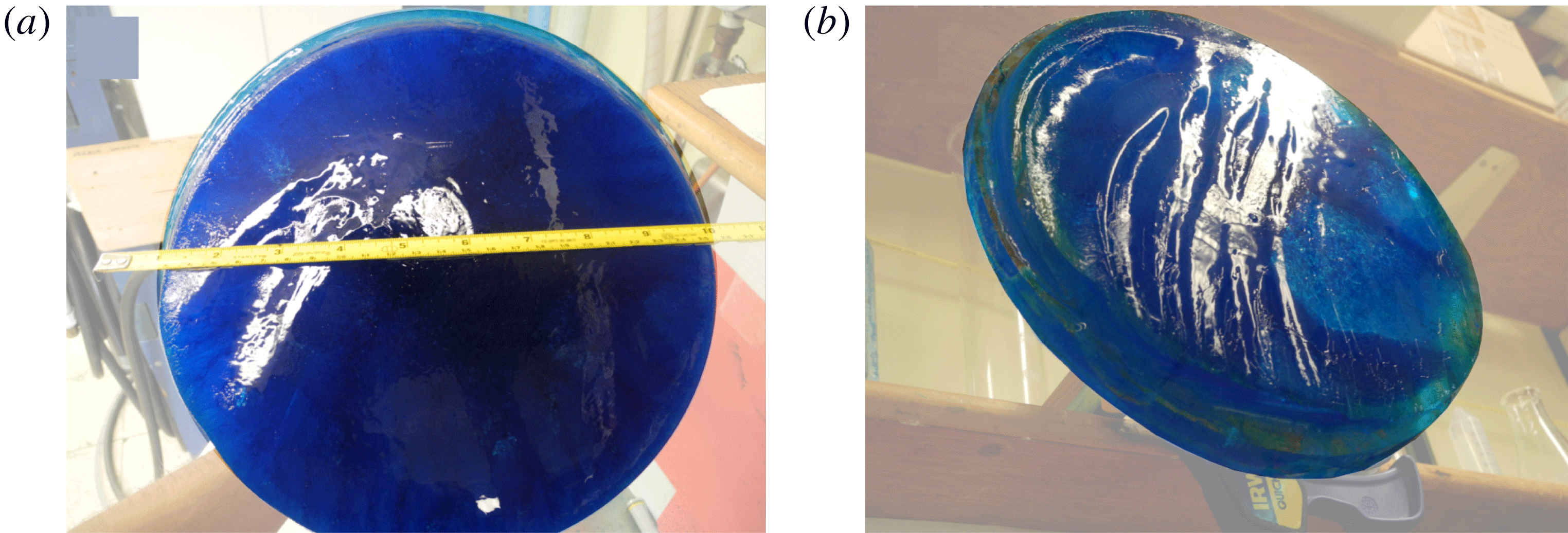
The increased melt rate for high background rotation was also observed in the laboratory by visual inspection of the base of the ice block at the end of the experiments, as shown in figure 7. Comparing two experiments with the same free stream velocity
 $U$
but different background rotation
 $f$
, it was clear that in the case of higher rotation (lower
 $\unicode[STIX]{x1D6FC}$
) the basal melting was higher than in the case of lower background rotation (higher
 $\unicode[STIX]{x1D6FC}$
). In particular, in the case of high background rotation, a region of higher melting, in forms of elongated stripes roughly along the curved streamlines of the steady-state solution and outside the TC region, was observed.
Two pictures of the bottom of the ice blocks after two experiments with the same free stream velocity
 $U=4~\text{cm}~\text{s}^{-1}$
and different background rotation: (a) low
 $f$
,
 $\unicode[STIX]{x1D6FC}>\unicode[STIX]{x1D6FC}_{c}$
and (b) high
 $f$
,
 $\unicode[STIX]{x1D6FC}<\unicode[STIX]{x1D6FC}_{c}$
. In (b) a partial TC was observed. When submerged, the rightward side of the ice blocks in these images was closest to the axis of rotation of the tank.
To resolve the discrepancy between the experimental melt rates and the corrected WC parametrization, there are a few other dynamical aspects that should be considered: for example, the meltwater gravity current dynamics at the base of the ice block, the effects of the meltwater on the TC dynamics through changes in the stratification, which are known to introduce a dependence of the velocity on the vertical distance from the obstacle (Huppert Reference Huppert1975), the curvature of the streamlines due to the geometrical shape of the tank, the transient features of the flow response and an accurate description of the flow changes due to the fact that the obstacle is finite (within the fluid).
Another aspect of the theory that needs further work is the assumption that the side and basal melt rate,
 $\dot{v}_{s}$
and
 $\dot{v}_{b}$
, are equal. Here, this assumption is based on some considerations following the work of Eckert & Drake (Reference Eckert and Drake1959). In fact, by estimating the side melt rate using the turbulent heat flux for a flow past a cylinder and by estimating the basal melt rate using the flux for a flow past a flat plate, one can calculate the ratio of the two melt rates. In particular, this means that the parameters
 $K$
,
 $m$
and
 $n$
that appear in (2.1) and (2.2) are different for the side and basal melt rates. This results in the ratio
 $\dot{v}_{s}/\dot{v}_{b}$
being 1.06, 0.93 and 0.87 for
 $U=2$
, 4 and
 $6~\text{cm}~\text{s}^{-1}$
, respectively. Some estimates of
 $\dot{v}_{s}$
and
 $\dot{v}_{b}$
by image analysis of the pictures of the ice blocks taken before and after the experiments are in agreement with the assumption that the two melt rates are of the same order (not shown). Since this method has large uncertainties, the ratio
 $\dot{v}_{s}/\dot{v}_{b}$
could not be constrained further to improve the analysis. An additional factor to bear in mind, as discussed below, is that the finite height of the obstacle alters the flow structure and, thus, the heat transfer to the ice block and, ultimately, its melting.
In what follows, a discussion is added about the fact that in the derivation of the interior flow solution neither Ingersoll (Reference Ingersoll1969) nor Johnson (Reference Johnson1983) include the description of the flow near the edges of a finite cylindrical obstacle. In the extreme case of a TC fully extended over the base of the obstacle, for
 $Ro\ll 1$
, the flow is two-dimensional and always goes around the motionless portion of fluid under the obstacle, i.e. the TC. Instead, if the background rotation is negligible, for
 $Ro\gg 1$
, the flow has a three-dimensional structure near the edge of the obstacle, with a fraction of the fluid going under it and the remaining fraction going around it. Thus, the assumption that the velocity field is two-dimensional and independent of the height may not hold even in the intermediate case of
 $Ro\sim 1$
, as in the experiments of this work. This has a clear parallel in the problem of stratified flow over a mountain, where the stratification is acting to suppress vertical motion, but in the vicinity of the topography there is a region of three-dimensional motion with part of the fluid going over the mountain (Greenslade Reference Greenslade, Castro and Rockcliff1994). In the present case, the thickness of this layer is expected to scale with
 $Ro$
or
 $\unicode[STIX]{x1D6FC}$
, so that it gets small in the limit of vanishing
 $Ro$
.
The fact that some fluid flows under the ice block rather than around it is not included in the corrected WC parametrization and if a fraction of fluid is added beneath the obstacle, it means that the flow is accelerated at the base of the cylinder, for conservation of mass. Since the ice melt rate is based on the velocity field immediately below the ice block, this acceleration might affect its melting.
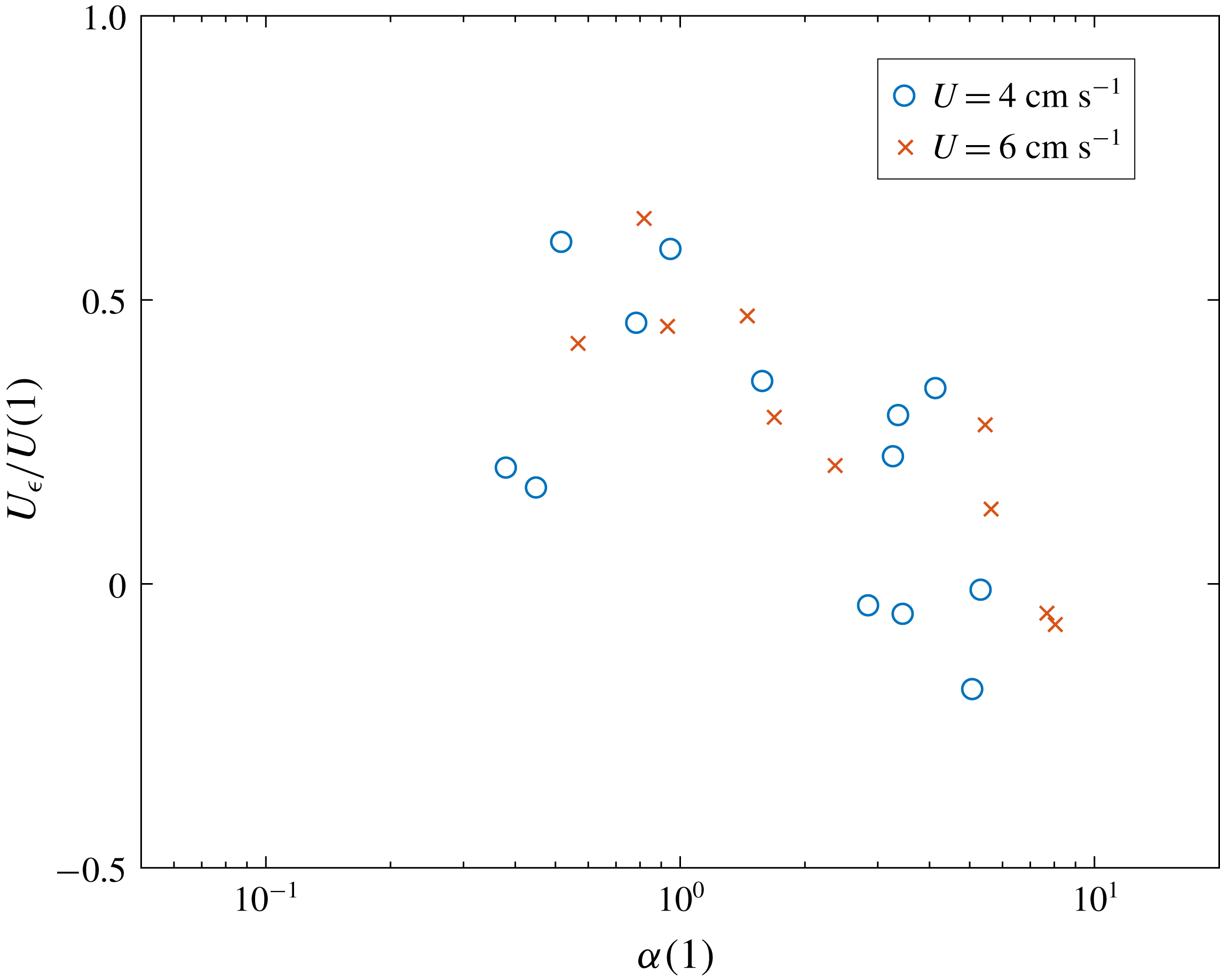
A simple attempt to quantify this process is now introduced. An additional velocity
 $U_{\unicode[STIX]{x1D716}}=U_{\unicode[STIX]{x1D716}}(\unicode[STIX]{x1D6FC})$
is added to the free stream velocity
 $U$
, so that the WC parametrization calculated with the corresponding
 $\overline{U}$
matches the experimental data. The non-dimensional extra velocity
 $U_{\unicode[STIX]{x1D716}}/U$
is shown in figure 8 as a function of
 $\unicode[STIX]{x1D6FC}$
for
 $U=4~\text{cm}~\text{s}^{-1}$
and
 $U=6~\text{cm}~\text{s}^{-1}$
. The series with
 $U=2~\text{cm}~\text{s}^{-1}$
is excluded because its dynamics seems to be controlled by the meltwater gravity current that forms at the base of the block. Unfortunately, at this stage, it is not possible to determine if the dependence on
 $\unicode[STIX]{x1D6FC}$
is due to more fluid being swept under the block or to the accelerated layer being confined to a thinner height under the block, because the full three-dimensional flow is not known. Therefore, more work is encouraged to investigate the behaviour of a rotating flow past a finite cylinder as a function of
 $Ro$
or
 $\unicode[STIX]{x1D6FC}$
.
Normalized extra velocity
 $U_{\unicode[STIX]{x1D716}}/U$
as a function of
 $\unicode[STIX]{x1D6FC}$
.
To address the open issues highlighted above, apart from performing new experiments in the laboratory, one could also think of some direct numerical simulations of the flow past an ice block. Numerical simulations of ice melting face several complications due to the small but important turbulent boundary layer near the ice–fluid interface and the evolving boundary. Nonetheless, they would be a useful tool to determine the three-dimensional flow field around the obstacle and the partial TC.
5 Conclusions
Through laboratory experiments in a rotating tank with cylindrical ice blocks mimicking Antarctic tabular icebergs, the effects of the Earth’s rotation on iceberg melting were investigated. It is found that at high rotation rates the base of the ice block melts more rapidly because of an increased average basal velocity below the block itself. This results from the enhanced relative vorticity below the block following the squeezing of the fluid column in the rotating system. In contrast, at low background rotation, the fluid flow is almost unaffected. When increasing the rotation, i.e. lowering
 $\unicode[STIX]{x1D6FC}$
, the ratio of the Rossby number to the non-dimensional height of the obstacle, the TC starts forming on one side of the obstacle and partially covers its base. In this condition, where the TC is not present, the flow velocity is larger than the far-field value, which is thought to be responsible for the observed higher melting. As the background rotation is further increased, i.e. for lower
 $\unicode[STIX]{x1D6FC}$
, the TC extends its area until it covers the entire ice block base. It is expected, then, that the melt rate is no longer dependent on the rotation rate, because the TC structure is unchanging.
The WC parametrization is then applied to describe the trend of the melt rate as a function of the free stream velocity
 $U$
. It is observed that for low relative velocity, below a certain threshold
 $U_{t}$
, the basal melt is not controlled by the forced convection due to
 $U$
, but it is controlled by a gravity current formed by the buoyant meltwater pool spreading radially towards the edge of the ice block. More work is needed to understand better what is happening in this region, both in a non-rotating environment and in a rotating one. However it is clear that for low
 $U$
, the free stream velocity does not control the melting.
Two corrections have been made to the WC parametrization to add the TC dynamics and the observed change in regime at low relative free stream velocity. First, rotational effects are included by considering the analytical steady solution obtained by Johnson (Reference Johnson1983) for the TC problem under a cylindrical obstacle. Second, wherever the analytical velocity magnitude falls below the threshold velocity
 $U_{t}$
, it is replaced by
 $U_{t}$
itself. This represents the fact that the ice melt rate does not vanish for vanishing free stream velocity, because the heat transfer from the fluid to the ice is controlled by the meltwater gravity current dynamics. The WC parametrization calculated with
 $\overline{U}$
, the area average of the corrected velocity field at the base of the ice block, correctly reproduces the increasing melt rate trend for decreasing
 $\unicode[STIX]{x1D6FC}$
, for all the series of experiments. By looking at such a trend in the experimental data, the inclusion of rotational effects thus determines a 30–40 % relative increment of the melt rate.
Despite additional dynamics still needing to be considered, the present work shows that moderate background rotation characterized by
 $\unicode[STIX]{x1D6FC}\sim 1$
can significantly increase the basal melting of an ice block due to modifications of the flow typical of a rotating system and that for low relative free stream velocity the basal melt is not controlled by the free stream velocity. The first-order dynamics is understood and the increasing trend of the melt rate for decreasing
 $\unicode[STIX]{x1D6FC}$
observed in the data is reproduced by the corrected WC parametrization. There are two key results that apply in the realistic ocean case,
 $\unicode[STIX]{x1D6FC}\sim 0.1$
. It is found that a TC is likely to form under a significant portion of the iceberg. Within this region, the melt rate is controlled by a gravity current like flow of buoyant meltwater towards the edge of the iceberg. Outside the TC region, the velocity is significantly higher than the free stream velocity due to the deflection of the ambient fluid around the TC. Within these regions, the melt rate is higher than predicted by the WC parametrization. This is likely to result in an asymmetric melt rate pattern inside and outside of the TC region. More work examining the structure of the flow past a finite cylinder as a function of
 $Ro$
together with the meltwater gravity current dynamics at the base of the ice block is encouraged for further developments.
Acknowledgements
The authors acknowledge A. Jensen for his help in building the apparatus and the ice block moulds and the GFD Summer Program held at Woods Hole Oceanographic Institution where the work was undertaken. A.N.M. was funded by the 2017 GFD Summer Program Fellowship and thanks C. Pasquero for her continuous scientific encouragement and support. C.D.M. acknowledges funding from the Weston Howard Jr Fellowship. C.C. was supported by NSF OCE-1658079.



