


Concern over the political consequences of misperceptions and misinformed beliefs has steadily escalated in recent years. In contrast to ignorance of the truth, misperceptions are distinguished by the depth, firmness, steadfastness, or confidence with which one holds a false or unsupported belief (Flynn, Nyhan, and Reifler Reference Flynn, Nyhan and Reifler2017; Kuklinski et al. Reference Kuklinski, Quirk, Jerit, Schwieder and Rich2000). This prevailing definition of a misperception falls in tension with classic research on attitudes, which holds that survey responses are best characterized as on-the-spot inferences based on whatever relevant information the respondent can call to mind (Tourangeau, Rips, and Rasinski Reference Tourangeau, Rips and Rasinski2000; Zaller Reference Zaller1992). In an effort to close the gap between definitions and measurement, a growing body of research advocates reserving the term “misperception” or “misinformed” for those who report a high level of confidence or certainty about their response (e.g., Graham Reference Graham2020; Kuklinski et al. Reference Kuklinski, Quirk, Jerit, Schwieder and Rich2000; Luskin, Sood, and Blank Reference Luskin, Sood and Blank2018; Pasek, Sood, and Krosnick Reference Pasek, Sood and Krosnick2015; Peterson and Iyengar Reference Peterson and Iyengar2021). At face value, certainty scales would seem to bridge the gap between the beliefs of interest and the vagaries of the survey response. Yet no published research interrogates the veracity of survey respondents’ claims to be certain of falsehoods.
This paper examines the nature of the beliefs captured by survey measures of misperceptions. It does so by adapting the long tradition of using temporal stability to interrogate the degree to which survey responses reflect true attitudes or beliefs (Converse Reference Converse and Apter1964; Reference Converse and Tufte1970). As opposed to confidently held beliefs, prevailing practices are more aptly characterized as capturing a mix of blind guesses and “miseducated” guesses based on mistaken, on-the-spot inferences. In five surveys covering a range of topics from existing research—government budgets, politicized controversies, the economy, science, and the COVID-19 pandemic—respondents who initially endorse falsehoods exhibit a large regression to the mean effect in follow-up surveys, assigning far less probability to the falsehood than their initial response implied. Respondents who answer the same questions correctly exhibit three to five times less regression. This result holds even among those who report 100% certainty. Whereas the average respondent who reports complete certainty about a correct answer assigns an average probability of around 0.95 to their initial response in a follow-up survey, the average respondent who reports complete certainty about an incorrect answer drops to about 0.75. This means that even the typical respondent who claims to be absolutely certain of falsehoods is not deeply convinced of the statement they have endorsed. Instead, they find the falsehood to be more plausible than not based on underlying beliefs that are suggestive, but not dispositive, as to the matter in question.
Any framework capable of describing a problem can also be used to evaluate solutions. As a step in this direction, the analysis concludes by evaluating a novel intervention that merges frame of reference training (FOR; Bernardin and Buckley Reference Bernardin and Buckley1981; Woehr Reference Woehr1994) with theories of the survey response (Tourangeau, Rips, and Rasinski Reference Tourangeau, Rips and Rasinski2000; Zaller Reference Zaller1992). Respondents read four short vignettes about a hypothetical person answering a question about the price of gas, guess that person’s certainty level, and then receive instruction as to which certainty level is most appropriate and why. This 60–90-second exercise increases the temporal stability of measured misperceptions by about 40%. These benefits extend to both high and low respondents on several dimensions that have previously been shown to predict incorrect answers to survey questions and real-world engagement with misinformation—for example, partisan identity and cognitive reflection.
The findings suggest three principles for building a sounder evidentiary basis for understanding the prevalence and consequences of misperceptions. First, interpretations of survey measures can and should be justified with hard empirical evidence. Even as the results yield little evidence of firm belief in falsehoods, the same measurement techniques identify firm, confidently held beliefs among those who report being certain of the correct answers of a multiplicity of questions designed to tap political and scientific knowledge. It cannot be taken for granted that a survey question has measured misperceptions, but it can be proven. Second, theoretical expectations as to who is most likely to be misinformed are a poor substitute for hard evidence. The results hold when samples are split by dispositions that existing research has shown to predict incorrect answers to survey questions and real-world engagement with misinformation, including political party, generic conspiracy beliefs, and need for cognitive closure. Third, evidence on measurement properties should be question specific. Though this paper finds modest degrees of response stability among incorrect answers to some questions, others are unstable across the board. For example, denial that global temperatures have risen appears to be almost entirely driven by blind guessing, with extremely low response stability even among those who report complete certainty. Similar measurement properties are observed among those who deny the existence of continental drift.
The lack of correspondence between prevailing interpretations of measured misperceptions and their observable measurement properties calls for a reassessment of existing evidence as to the prevalence, predictors, and consequences of misperceptions and misinformed beliefs. Political partisanship may be the most studied predictor of incorrect survey responses. This paper’s findings suggest that measured partisan belief differences should be interpreted not as evidence of misperceptions but as differential knowledge and ignorance of convenient and inconvenient truths. As elaborated in the concluding section, this posture is consistent with several established patterns that misinformation-focused accounts have trouble accommodating. The findings also call for reconsideration of research on correcting misperceptions and the benefits (or lack of benefits) that arise from doing so. Much of this research is unlikely to have measured misperceptions to begin with and is more safely interpreted as describing the consequences of ignorance.
Though the results are discouraging for the unvalidated measurement practices that dominate existing survey-based research on political misperceptions, this paper’s ultimate value lies in its development of methods for identifying relatively successful questions and measurement practices. By assuming the burden of proof for its interpretation of survey responses, research can develop a more trustworthy basis for understanding the prevalence and consequences of political misperceptions.
A Conceptual–Empirical Disconnect
Surveys are commonly used to document “widespread” misperceptions and misinformed beliefs among the general public as well as what personal characteristics predict such beliefs, how to correct them, and the consequences of doing so (Flynn, Nyhan, and Reifler Reference Flynn, Nyhan and Reifler2017, 129; Nyhan Reference Nyhan2020, 227). Misperceptions are distinguished from ignorance by the degree of conviction with which the respondent holds the belief (Kuklinski et al. Reference Kuklinski, Quirk, Schwieder and Rich1998; Reference Kuklinski, Quirk, Jerit, Schwieder and Rich2000). Whereas the “genuinely misinformed” “firmly hold beliefs that happen to be wrong,” the “guessing uninformed” “do not hold factual beliefs at all” (Kuklinski et al. Reference Kuklinski, Quirk, Jerit, Schwieder and Rich2000, 792–3). Consistent with this influential distinction, research describes misperceptions and misinformed beliefs as “firm” (Jerit and Zhao Reference Jerit and Zhao2020, 78, 81), “deep-seated” (Berinsky Reference Berinsky2018, 212), “steadfast” (Li and Wagner Reference Li and Wagner2020, 650), “confidently held” (Pasek, Sood, and Krosnick Reference Pasek, Sood and Krosnick2015) “belief in information that is factually incorrect” (Berinsky Reference Berinsky2018, 212), which can be thought of as “incorrect knowledge” (Hochschild and Einstein Reference Hochschild and Einstein2015, 10). Though the terms “misperception” and “misinformation” are often used interchangeably,Footnote 1 this paper favors the former so as to maintain a clear distinction between beliefs and the information environment (also see Thorson Reference Thorson2015).
Researchers’ interest in beliefs of this kind runs into a classic problem in the study of public opinion: respondents answer survey questions even when they do not hold a firm belief about the matter at hand. Converse (Reference Converse and Apter1964; Reference Converse and Tufte1970) famously pointed out that many responses are temporally unstable, meaning that they change from one survey to the next. To accommodate this and other empirical regularities that problematize the idea that surveys measure preexisting beliefs (e.g., Schuman and Presser Reference Schuman and Presser1981), researchers developed alternative accounts. Consensus now holds that survey-measured attitudes are generally not firm, deep, or steadfast but are formed by retrieving a “sample” of topic-relevant considerations from memory and integrating them into an on-the-spot judgment (Strack and Martin Reference Strack, Martin, Hippler, Schwarz and Sudman1987; Tourangeau, Rips, and Rasinski Reference Tourangeau, Rips and Rasinski2000; Zaller Reference Zaller1992; also see Berinsky Reference Berinsky2017; Bullock and Lenz Reference Bullock and Lenz2019; Flynn, Nyhan, and Reifler Reference Flynn, Nyhan and Reifler2017).
In an effort to close the gap between the definition of a misperception and the received wisdom from attitudinal research, some research applies a higher standard of measurement. Research increasingly uses certainty or confidence scales to identify respondents who are misinformed or hold a misperception (Flynn Reference Flynn2016; Graham Reference Graham2020; Lee and Matsuo Reference Lee and Matsuo2018; Li and Wagner Reference Li and Wagner2020; Marietta and Barker Reference Marietta and Barker2019; Pasek, Sood, and Krosnick Reference Pasek, Sood and Krosnick2015; Peterson and Iyengar Reference Peterson and Iyengar2021; Sutton and Douglas Reference Sutton and Douglas2020). Such research often finds that misperceptions or misinformed beliefs are much less common than is generally supposed. Luskin, Sood, and Blank (Reference Luskin, Sood and Blank2018) refer to certainty scales as a “24-carat gold standard” for measuring misinformed beliefs. Accordingly, the 2020 American National Election Study added a “misinformation” battery that included a confidence scale of this kind.
At face value, one who reports being certain of a falsehood would seem to firmly believe it. Yet there also exists suggestive evidence that respondents may claim to be certain of falsehoods that are not firmly believed. Alongside questions designed to tap partisan-biased misperceptions, Graham (Reference Graham2020) measures confidence in answers to political knowledge questions about officeholders and institutional rules. About one in 10 respondents reported being “very” or “absolutely” certain about an incorrect answer. Graham (Reference Graham2020) attributes this to “traps” set by the response options—for example, “Nancy Pelosi as the Senate Minority Leader (instead of Chuck Schumer)” and “the filibuster as the Senate procedure to make budget changes via a simple majority (instead of reconciliation)” (318). Few would interpret these responses as representing beliefs that are firm, deep, steadfast, or related in any way to misinformation.
Further reasons to be skeptical that self-described certainty indicates a firmly held belief emerges from the literature on attitude strength. The few published tests of the strength–stability relationship find that strong attitudes are only modestly more stable than weak attitudes, with little focus on exactly how strong the strongest attitudes are. In a 1974–75 panel survey, Schuman and Presser (Reference Schuman and Presser1981) find that about 75% of high-importance respondents chose the same response to a binary item in both survey waves, compared with 65% in the low-importance group. Krosnick (Reference Krosnick1988) finds a weak (“not strong,” 243, 247) relationship on six items in the 1980–88 ANES. Reanalyzing a larger subset of the same data, Leeper (Reference Leeper2014) finds statistically significant relationships for three of the six items. In three other datasets, Leeper (Reference Leeper2014) finds only a weak relationship. Prislin (Reference Prislin1996) conducts 14 regression tests for each of three attitudinal scales and found one statistically significant relationship in each case. Evidence also emerges that the strength–stability relationship is heterogeneous. Krosnick (Reference Krosnick1988) finds the strongest attitudes toward unemployment to be less stable than the weakest attitudes toward other issues. Bassili (Reference Bassili1996) finds a stronger relationship with respect to pizza than to any policy issue, and finds no relationship with respect to attitudes toward pornography. Schuman and Presser (Reference Schuman and Presser1981) find that among opponents of gun control, attitude strength strongly predicts self-reported activist behavior; among supporters, the relationship is completely flat.Footnote 2
If incorrect answers to survey questions do not represent firm, deep, or steadfast misperceptions, what else could they represent? The analysis considers two other archetypes: blind guesses and miseducated guesses. Blind guessers either do not possess or do not put much effort into recalling topic-relevant considerations. Such respondents should split evenly between response options as though the respondent is flipping a mental coin. Miseducated guesses are made by respondents who sample their considerations from a pool of stored information that favors one response option over the others but is not conclusive as to which is true or which is false. Such respondents may make the same guess with regularity but do not firmly believe the falsehood implied by their incorrect answer. For example, a respondent may reason that a true claim about Trump is false because they believe that media are always making up stories about him (see Table 2 and the surrounding discussion). Relative to blind guessers, miseducated guessers are characterized by a greater degree of latent ambivalence, meaning that their memory contains topic-relevant considerations that point in both directions. In moments when the most accessible considerations happen to all point in one direction, such respondents may have a fleeting feeling of confidence that is not representative of their true beliefs. In other moments, the same respondents may feel uncertain or even make the opposite guess as to which response option is most likely to be correct.
Regression to the Mean, Study 2

Note: The table displays the statistic named in the column header for each question in Study 2, and c
i1 and b
i2 are defined in the text. The “Diff” column displays c
i1
 $ - $
b
i2, and “D-in-D” column displays the difference between the “Diff” columns. Clustered standard errors in parentheses. N = 866.
Examples of Miseducated Guesses, Study 2a

In the language of the attitudinal literature, an educated or miseducated guess can be thought of as a middle category between Converse’s (Reference Converse and Apter1964; Reference Converse and Tufte1970) famed limiting cases of a nonattitude and a crystallized belief. Researchers have long recognized that a “third concept” like “quasi-attitudes or pseudo-attitudes” would aptly describe many responses (Schuman and Presser Reference Schuman and Presser1981, 159). Even Converse’s seminal articles (Reference Converse and Apter1964; Reference Converse and Tufte1970) found that a “black-and-white” distinction between nonattitudes and crystallized attitudes applied to only one of eight attitudinal questions; for the other seven, intermediate response types were “entirely compatible with the data” (Reference Converse and Apter1964, footnote 41).Footnote 3 Attitudinal research ultimately adapted by merging the middle and top categories, lowering the bar for “attitudes” to include on-the-spot judgments (Tourangeau, Rips, and Rasinski Reference Tourangeau, Rips and Rasinski2000; Zaller Reference Zaller1992) formalized as latent variables that exist by definition (Achen Reference Achen1975; Erikson Reference Erikson1979; see discussion below). For misperceptions and beliefs more generally, a three-category conceptualization adds value for two reasons. First, far from giving up on the top category, research often claims to have measured deep, firm, steadfast belief in specific falsehoods. Second, as this paper shows, certainty scales do enable firmly held beliefs to be measured for a wide range of items—but only among those who answer correctly. Unlike the case of attitudes, ruling out the possibility that surveys measure firm beliefs is not an option. Instead, research on beliefs and misperceptions needs clear language to distinguish the firmly held beliefs it wants to measure from the mis/educated guesses it often measures instead.
Though archetypes are expositionally useful, the analysis ultimately refrains from anointing any particular certainty level as distinguishing one type of belief from another. The arbitrariness of choosing such thresholds is deep enough that philosophers generally reject threshold-based conceptions of belief altogether (Foley Reference Foley1992). Instead, the empirical framework below specifies two benchmarks against which to judge claims to be certain about incorrect answers: what would be observed in the absence of measurement error and what is actually observed among correct answers collected in the same survey using the same measurement technique. This gives a sense of where responses fall along the continuum without resorting to sharp, ultimately arbitrary distinctions. The frequent focus on respondents who claim to be 100% certain of their answers is intended not as an implicit threshold but as a most likely case for measuring misperceptions as they are traditionally defined—and by extension, as a least likely case for this paper’s main result.
The task at hand is distinct from two related lines of research. First, as mentioned above, several articles note that apparent misperceptions drop substantially when measures of confidence or certainty are incorporated. This paper focuses not the prevalence or predictors of such responses but on how to interpret them. Second, other research examines expressive responding, which is survey subjects’ tendency to select responses other than their sincere best guess as a way of expressing partisan sentiments (Berinsky Reference Berinsky2018; Bullock et al. Reference Bullock, Gerber, Hill and Huber2015; Prior, Sood, and Khanna Reference Prior, Sood and Khanna2015). The only study of expressive responding that includes measures of certainty does not probe the veracity of claims to be certain (Peterson and Iyengar Reference Peterson and Iyengar2021). Some studies of expressive responding allow respondents to say “don’t know” (DK), which tends to filter out respondents with low levels of knowledge (Luskin and Bullock Reference Luskin and Bullock2011; Sturgis, Allum, and Smith Reference Sturgis, Allum and Smith2008) and certainty (Graham Reference Graham2021). This means that DK response options are well suited to filtering out blind guesses, but they do not isolate a group of respondents that firmly believes its answers.Footnote 4
Empirical Framework
Research contending that surveys measure true attitudes has long represented survey responses as functions of probability distributions consisting of a true attitude and an error term (Achen Reference Achen1975; Ansolabehere, Rodden, and Snyder Reference Ansolabehere, Rodden and Snyder2008; Erikson Reference Erikson1979). The “true” attitude or belief is a latent variable that exists by definition.Footnote
5
For a binary question (with two response options), define respondent i’s spontaneously formed belief as
 $ \tilde{p}_i\equiv {p}_i+{\epsilon}_{it} $
, where
 $ {p}_i\,\in\,\left[0,1\right] $
is i’s true belief and
 $ {\epsilon}_{it} $
is error in the measure taken at time t. When
 $ {p}_i=1 $
, i holds a completely certain belief in the correct answer. When
 $ {p}_i=0 $
, t holds a completely certain belief in the incorrect answer. Accordingly, define i’s stated best guess as the response they claim to find most probable,
 $ \tilde{g}_{it}\equiv 1\left(\tilde{p}_{it}>0.5\right) $
. Define certainty as the probability i assigns to their best guess, which can be written as,
 $ \tilde{c}_{it}\equiv argmax\left(\tilde{p}_{it},1 - \tilde{p}_{it}\;\right) $
. Existing research on factual beliefs adopts similar models with no explicit error term (Bullock et al. Reference Bullock, Gerber, Hill and Huber2015; Bullock and Lenz Reference Bullock and Lenz2019).Footnote
6
To quantify response stability, the analysis will examine what belief is expressed in a follow-up survey conditional on what belief was expressed initially. Figure 1 displays two ways of visualizing this relationship. First focusing on the left panel, define the conditional average belief as
 $ \unicode{x1D53C}\left[{\overset{\sim }{P}}_{i2}, |,\;{\overset{\sim }{P}}_{i1}=p\right] $
, where
 $ \unicode{x1D53C} $
, the expectation operator, simply takes the average. If
 $ {\epsilon}_{it} $
is unsystematic and uncorrelated over time,
 $ \unicode{x1D53C}\left[{\overset{\sim }{P}}_{i2}, |,\;{\overset{\sim }{P}}_{i1}=p\right] $
is an unbiased estimate of the true belief, pi
, conditional on the belief reported at t = 1. Absent measurement error, the first and second measures of belief would always line up exactly.Footnote
7
In Figure 1, this is visualized by the dashed line that cuts a 45-degree line across the left panel. When beliefs are measured with error, they depart from this ideal. This is represented by the solid line, which is stylized after the results.
Two Ways to Display the Temporal Stability of Respondents’ Measured Beliefs

As some error is to be expected in all survey measures, it is more charitable to benchmark incorrect answers against a certifiably attainable goal: the degree of stability observed among respondents who claim the same degree of certainty about correct answers. This provides a sense of whether instability among incorrect beliefs could be an artifact of the certainty scale’s limitations. To facilitate such comparisons, Figure 1’s right panel introduces an alternative display for the same data. Intuitively, the right panel “folds” the left panel both vertically and horizontally, mirroring the bottom-left quadrant onto the top right. The close alignment between the dashed lines indicates that absent measurement error, the beliefs of respondents who answered correctly and incorrectly should be equally stable. The gap between the solid lines previews the paper’s primary result: conditional on how certain a respondent claims to be, incorrect beliefs are less stable than correct beliefs. Formally, define belief stability as
 $$ {\displaystyle \begin{array}{c}\hskip-2.2em {b}_{i2}=\hskip1em {c}_{i2}\hskip1em \mathrm{if}\hskip1em {g}_{i1}=\hskip.1em {g}_{i2\hskip-.1em }\\ {}1 - {c}_{i2}\hskip1em \mathrm{if}\hskip1em {g}_{i1}\ne {g}_{i2}\end{array}} $$
and conditional belief stability as
 $ \unicode{x1D53C}\left[{B}_{i2}\;|\;{C}_{i1}=c\right] $
. This faithfully reflects the stability of each respondent’s measured belief while facilitating direct comparisons between respondents’ degree of belief in correct and incorrect answers.
A useful interpretation of
 $ \unicode{x1D53C}\left[{B}_{i2}\;|\bullet \right] $
is the average respondent’s true degree of belief in their initial best guess. Just as
 $ \tilde{p}_{i1}=\tilde{p}_{i2} $
when beliefs are measured without error, it follows directly from (1) that an error-free measure of belief would mean that
 $ \tilde{b}_{i2}=\tilde{c}_{i1} $
.Footnote
8
Differences between
 $ \tilde{b}_{i2} $
and
 $ \tilde{c}_{i1} $
indicate that measurement error systematically inflated (or deflated) the apparent degree to which respondents believe their chosen answer. Accordingly, differences between
 $ {b}_{i2} $
and
 $ {c}_{i1} $
will sometimes be referred to as regression to the mean.
For some readers, it may help to relate the plotted quantities to predicted values from an ordinary least squares regression. Observe that
 $ \unicode{x1D53C}\left[{B}_{i2}\;|\;{C}_{i1}=c\right] $
is a conditional expectation function (CEF). Predicted values from a regression approximate the CEF under the assumption that
 $ \unicode{x1D53C}\left[Y|X=x\right] $
is linear in X (Angrist and Pischke Reference Angrist and Pischke2008; Aronow and Miller Reference Aronow and Miller2019). This means that the plots in this paper provide the same information depicted in a typical plot of predicted values but without the ex ante assumption that stability is exactly linear in certainty. Appendices B.4 and C.4 show that the results hold within a regression framework.
Although the heart of the analysis focuses on belief stability, Study 1 considers certainty scales defined only in terms of subjective scale points. Such scales do not capture individual-level uncertainty in a way that aligns with distributions defined by probability theory.Footnote
9
For such data, the analysis examines a metric that may be more familiar to consumers of survey research: the stability of the respondent’s best guess. Define best guess stability as
 $ {s}_{i2}\equiv 1\left({g}_{i1}={g}_{i2}\right) $
, which equals 1 if the respondent’s best guess in the second survey matches the best guess in the first survey and 0 if the two guesses do not match. In analysis of a survey that elicited only the respondent’s best guess about each question, si
would be called “response stability.” For the present analysis, it has two main disadvantages. First, si
is completely insensitive to cases in which best guesses are stable but certainty is not. Second, an error-free measure of best guesses would always be perfectly stable, regardless of the respondent’s level of certainty. As properties of a performance measure, “insensitive to a crucial source of variation” and “uninformative expectations” are not great. Despite these shortcomings, the appendices to Studies 2 and 3 show that similar results obtain when best guess stability is substituted for belief stability.
Threats to Inference
The analysis takes steps to mitigate four sources of measurement error that could artificially inflate differences in stability between correct and incorrect answers. First, respondents could look up the correct answers while taking the survey. Accordingly, each survey included at least one established method of detecting and deterring information search. Second, differences between correct and incorrect answers could be an artifact of scale coarseness. Coarse scales ask respondents with a range of latent certainty levels to group themselves together into the same bin, potentially creating an artificial gap between correct and incorrect answers. For example, it could be that most of those who answer correctly and choose the highest certainty level are close to 100% certain, whereas most of those who answer incorrectly and choose the highest level intend to claim only 70% or 80% certainty. Whereas Study 1 uses scales from previously published research, Studies 2 and 3 account for concerns about coarseness by using more-granular scales. Third, respondents’ true beliefs may genuinely change between waves of the survey. If the information that causes such changes disproportionately favors the correct answer, an asymmetry between correct and incorrect answers could emerge as a consequence. Fourth, it could be that expressive responding occurs in both waves, artificially inflating the stability of incorrect beliefs among respondents with a partisan incentive to endorse a falsehood (as well as correct beliefs about convenient truths).
To address the third and fourth threats, the results of Studies 2 and 3 are reproduced using an alternative, incentive-compatible measure of belief. The costly measure collects the same information as a direct question using a series of choices between payment for a correct answer and fixed probabilities of earning the same reward.Footnote 10 Measuring the belief twice in the same survey using two distinct measures mitigates concerns that the results are an artifact of change between surveys.Footnote 11 The financial incentive mitigates the concern that expressive tendencies, not the beliefs themselves, drive belief stability and partisan differences therein.
The costly measure proceeds as follows. At the outset, respondents are told that they will make a series of choices between tickets to enter into drawings for bonus payments of up to $100. On each screen, respondents first choose which of two tickets they would like to enter into the drawing: win if [choice A], or win if [choice B]. A menu of additional choices then appears: win if [selected choice] or an X in 10 chance to win. By choosing between winning if one’s best guess is correct and a 6 in 10, 7 in 10, 8 in 10, 9 in 10, and 99 in 100 chance to win, respondents reveal their probabilistic beliefs in an incentive-compatible manner. For example, one who would rather be paid for a correct answer than an 8 in 10 chance to win but prefers a 9 in 10 chance over payment for a correct answer, assigns a probability between 0.8 and 0.9 to their response. Hill (Reference Hill2017) uses a version of this approach to study beliefs about politically relevant facts. Holt and Smith (Reference Holt and Smith2016) find that discrete choice methods like this paper’s outperform methods that ask respondents to directly state their crossover probability (also see Trautmann and van de Kuilen Reference Trautmann and van de Kuilen2015).
Study 1: Foreign Aid
The U.S. government’s foreign aid budget is a classic case in research on misperceptions. In the 1990s, polling on the subject attracted sufficient attention that “the Clinton administration embarked on a major public relations effort focused on countering the American public’s overestimation of U.S. spending on foreign aid” (Kull Reference Kull2011, 57). Whereas foundational research interprets Americans’ incorrect answers to survey questions about foreign aid as representing ignorance (Gilens Reference Gilens2001), recent work heavily favors misperception and misinformation frames (Flynn Reference Flynn2016; Guay Reference Guay2021; Hochschild and Einstein Reference Hochschild and Einstein2015; Scotto et al. Reference Scotto, Reifler, Hudson and vanHeerde-Hudson2017; but see Lawrence and Sides Reference Lawrence and Sides2014).
This section introduces the paper’s main finding using this classic case. The foreign aid question from the 2012, 2016, and 2020 ANES was embedded in the pretreatment background questions for an unrelated panel survey conducted on Lucid in August and September 2018 (wave 2 N = 1,749). To discourage information search, respondents were first asked to pledge not to cheat (Clifford and Jerit Reference Clifford and Jerit2016). Respondents were then asked, “On which of the following does the U.S. federal government currently spend the least?” and allowed to choose between four options, Foreign aid, Medicare, National defense, and Social Security.Footnote 12 As soon as the respondent answered, a five-point certainty scale appeared.Footnote 13 The scale’s wording was randomly assigned. Half of the respondents used the certainty scale from Graham (Reference Graham2020), whereas the other half used the certainty scale from Pasek, Sood, and Krosnick (Reference Pasek, Sood and Krosnick2015). The Graham scale asked respondents, “How certain are you that your answer is correct?” and used scale point labels ranging from “not at all certain” to “absolutely certain.” The Pasek scale asked, “How sure are you about that?” and used labels from “not sure at all” to “extremely sure.” The two scales had similar measurement properties and are pooled here for simplicity. Appendix B splits the results by scale.
In the first wave, 28.4% of respondents answered correctly. Average certainty was 2.92 among respondents who answered correctly and 2.83 among respondents who answered incorrectly (difference = 0.09, SE = 0.06). The small difference in certainty belies a larger difference in response stability. When recontacted 1 to 3 weeks later for the second survey, 65.1% of respondents who initially answered correctly chose the same best guess, compared with 48.6% of respondents who answered incorrectly (difference = 16.4, SE = 2.6). The share of respondents answering correctly held steady at 29.1%, suggesting that belief change between surveys is unlikely to have driven differences in response stability.
To examine the certainty scales’ success in identifying deeply held misperceptions, Figure 2 displays best guess stability conditional on certainty. The stability of correct answers rises with certainty, whereas the stability of incorrect answers is virtually flat. Because respondents were not offered a DK response option, there is a clear floor for response stability: if respondents were choosing completely at random, they would choose the same response option 25% of the time. Incorrect answers sit above this floor, falling near 50% regardless of the respondent’s certainty level. This suggests that incorrect answers reflect some tendency on the part of respondents to consistently retrieve similar considerations from memory as they form their on-the-spot judgment. However, the certainty scales did not capture much variation in this tendency.
Temporal Stability of Best Guesses by Certainty Level, Study 1
Note: The x-axis displays
 $ {c}_{i1} $
. The y-axis displays
 $ \unicode{x1D53C}\left[{S}_{i2}\;|\;{C}_{i1}={c}_{i1}\right] $
. The thin error bars represent 95% confidence intervals. The thick error bars represent 84% confidence intervals to aid comparisons between estimates; a lack of overlap between two such intervals suggests a statistically significant difference at p < 0.05, two-tailed (Julious Reference Julious2004). Appendix A presents these results in tabular form. N = 1,749.

Study 2: Politicized Controversies
Though Study 1 demonstrates that claims to be certain of falsehoods do not always indicate firmly held misperceptions, one may expect different results when it comes to salient political controversies. To gather such evidence, two original panel surveys were conducted on Amazon Mechanical Turk (MTurk). Study 2a was fielded in June 2019 and June 2020 (second wave N = 466). To discourage information search, it included a pledge not to cheat and an obscure “catch” question that would be difficult to answer correctly without looking it up (Clifford and Jerit Reference Clifford and Jerit2016). The first wave concluded with open-ended follow-up questions about how subjects came up with their answer to one randomly selected question. Study 2b was fielded on MTurk in March and August 2020 (second wave N = 420). It included a pledge not to cheat and a cheating detection method similar to those described by Diedenhofen and Musch (Reference Diedenhofen and Musch2017) and Permut, Fisher, and Oppenheimer (Reference Permut, Fisher and Oppenheimer2019). The first wave concluded with the costly measure of belief.
The surveys covered six politicized controversies, which were selected based on two criteria. First, partisan balance. Three questions’ incorrect answers are congenial to Democrats and three are congenial to Republicans. Second, prominent real-world misinformation. Four questions cover salient political controversies with prominent false claims in the public sphere, whereas two less prominent controversies (numbered 3 and 6 below) provide points of comparison. The questions with incorrect answers congenial to Democrats were
-
1. Clinton email. Respondents were asked whether the following is true or false: “While she was Secretary of State, Hillary Clinton used a private email server to send and receive classified information.” This was a central controversy during and after the 2016 presidential election campaign. Both before and after an FBI investigation revealed that Clinton had sent classified information, she falsely claimed that she had not.Footnote 14
-
2. Trump-Russia collusion. After a one-sentence description of the Robert Mueller’s special counsel investigation into Russian interference in the 2016 presidential election, respondents were asked whether the following is true or false: “Robert Mueller’s report stated that Trump personally conspired with Russia to influence the 2016 election.” Prior to the release of the report, many left-leading opinions claimed that Mueller would find such evidence.Footnote 15
-
3. Obama DAPA reversal. After a one-sentence description of Deferred Action for Parents of Americans (DAPA), a 2014 Obama initiative that was struck down in court, respondents were asked whether the following is true or false: “About a year earlier, Obama said that he would be ignoring the law if he issued such an order.” Obama said exactly this in a 2013 interview, but later denied changing his position.Footnote 16
The questions with incorrect answers congenial to Republicans were
-
4. Obama birth certificate. Respondents were asked whether the following statement is true or false: “President Obama has never released his birth certificate.” This question taps a clearly factual element of a larger conspiracy theory. Even after Obama released both his short- and later long-form birth certificates, demands that he do so continued to populate public discourse and social media.Footnote 17
-
5. Trump said “grab them.” Respondents were asked whether the following statement is true or false: “Before becoming president, Donald Trump was tape recorded saying that he kisses women and grabs them between the legs without their consent.” This was a major controversy in the 2016 presidential election campaign. After initially apologizing, President Trump later claimed that the tape was inauthentic.Footnote 18
-
6. Trump Article II. Respondents were told that Article II of the Constitution describes the President’s powers, then asked whether “President Trump has said that Article II gives him the power to do whatever he wants” is true or false. Trump has never disputed making this statement. This is the only question of the six that has not been the subject of prominent false claims.
After respondents chose their best guess, a certainty scale appeared. The scales were given probabilistic interpretations using both numerical labels (e.g., 50% to 100% certain) and three subjective anchors, “don’t know,” “probably [answer],” and “definitely [answer].” As a benchmark, three measures of the public’s general political knowledge (party control of the House of Representatives, John Roberts’ job, and Jerome Powell’s job) were included in Study 2b.
Regression to the Mean
Combining the two surveys, Table 1 introduces the data and examines subjects’ tendency to regress to the mean. On average, the percentage of correct answers was similar for the two sets of questions (first column). In the first survey, respondents who answered correctly assign an average probability of 0.88 and 0.85 to their answer, closer to a firm belief than a blind guess (second column). In the second survey, respondents regress slightly, assigning a probability of 0.83 and 0.79 to their initial response (third column). This regression to the mean of about 0.05 (fourth column) suggests that measurement error modestly overstates the extent to which correct answers represent firm, knowledge-like belief in the truth.
Incorrect answers exhibit greater regression. In the first survey, respondents who answer incorrectly assign an average probability of 0.70 and 0.74 to their answers (fifth column), which appears only somewhat closer to a blind guess than a confidently held false belief. In the second survey, respondents assign a probability of 0.55 and 0.55 to their initial responses (sixth column), a regression to the mean of about 0.15 on the knowledge questions and 0.19 on the controversy questions (seventh column). This is more regression than is seen among those who answered correctly (eighth column). Relative to correct answers, incorrect answers are less representative of deeply held beliefs.
These patterns are equally stark at the level of individual questions. For example, the average respondent who incorrectly states that Trump never said “grab them” reports a higher level of certainty than did the typical respondent who answered a general knowledge question incorrectly (0.77 versus 0.70). However, upon a second measure, respondents who initially endorse the false claim about Trump are no more committed to it than those who initially pick the wrong answer to political knowledge questions (0.53 versus 0.55). The highest average belief in one’s incorrect answer, 0.61 among those who at first said that Trump personally colluded with Russia, is three times closer to a blind guess (0.5) than to incorrect knowledge (1.0). In the remaining cases, the typical incorrect answer to the controversy items does not reflect any stronger a belief than does the typical incorrect answer to a political knowledge question.
Results by Certainty Level
Researchers use certainty scales in part to address their suspicion of what has just been shown—that incorrect answers do not reliably indicate deeply held misperceptions. To what extent do certainty scales succeed in closing this conceptual–empirical gap? Figure 3 plots belief stability conditional on the respondent’s wave-1 response (correct or incorrect) and their certainty level. This and all following figures bin the certainty scale as follows: 0.5, [0.51, 0.59], [0.6, 0.69], [0.7, 0.79], [0.8, 0.89], [0.9, 0.99], 1. Stability in the lowest and highest bins will frequently be significantly lower or higher than the adjacent bin, confirming the value of scale granularity.
Temporal Stability of Beliefs by Certainty Level and Question, Study 2
Note: The x-axis displays c
i1. The y-axis displays
 $ \unicode{x1D53C}\left[{B}_{i2}\;|\;{C}_{i1}={c}_{i1}\right] $
. Thin error bars represent 95% confidence intervals. The thick error bars represent 84% confidence intervals to aid comparisons between estimates (see note to Figure 2). Appendix B presents these results in tabular form. N = 886.

The controversy questions offer little evidence that incorrect answers to questions about partisan or politicized matters are reflective of firmly held beliefs (rightmost six panels, Figure 3). Among respondents who at first claim to be 100% certain of the incorrect answer, belief stability tops out at 0.80 among respondents who claim to be certain that Obama never said that an order like DAPA would amount to ignoring the law (third panel from left). However, this estimate is based on only seven respondents (all Democrats) and is not statistically distinguishable from blind guessing. The next-highest stability among the 100% certain and wrong comes on the Trump Article II question (0.76, second panel from right). Leaving aside those who report 100% certainty, the highest belief stability among any other subgroup is 0.66 among respondents who report being 90% to 99% certain that Mueller found personal collusion between Trump and Russia (Figure 3, middle panel).
This instability is not attributable to a flawed certainty scale. On the political knowledge questions, belief stability consistently comes close to the level that would be observed in the absence of measurement error (Figure 3, leftmost panel). Among respondents who report 100% certainty about the correct answer to these questions, belief stability reaches 0.98. Almost everyone who claims to be certain about facts like the identity of the Federal Reserve Chair appears to genuinely hold a firm, confident belief in the factual statement they endorse.
To make the results more concrete, Table 2 displays four selected respondents’ descriptions of how they came up with their answers. Prevailing uses of certainty scales would classify the respondents as holding a deeply held misperception in one of the two waves and as some other kind of belief in the other wave.Footnote
19
Although the respondents indicate some awareness of the controversy at hand, each also indicates that some heuristic helped them answer the question. Consider the Obama birth certificate respondent, a Republican. In the first wave
 $ {p}_{i1}=0.13 $
, meaning that the respondent chose the wrong answer (
 $ {g}_{i1}=0 $
) and reported 87% certainty (
 $ {c}_{i1}=0.87 $
). The respondent is not aware that Obama released his birth certificate but reasons that he must not have; if he had, there would be no controversy. In wave 2,
 $ {p}_{i2}=0.75 $
, meaning that the respondent selected the correct answer (
 $ {g}_{i2}=1 $
) and reported 75% certainty (
 $ {c}_{i2}=0.75 $
). Despite having a fair amount of confidence in their initial on-the-spot inference, this respondent reached a different conclusion the second time around.
On the surface, there is little to distinguish individuals who state low levels of certainty (around 0.5 to 0.7) from those who state moderate levels of certainty (around 0.7 to 0.9). A closer look suggests that low-certainty responses are characterized by a relatively stable tendency to select low levels of certainty, whereas moderate-certainty responses are more affected by a latent ambivalence that results in more response variability. To show this, Appendix B plots the variance in
 $ {b}_{i2} $
conditional on the respondent’s initial certainty level, c
i1—that is, Var(
 $ {B}_{i2} \mid {C}_{i1}=c $
); Appendix C does the same for Study 3. For both knowledge and controversy questions, second-wave variance is lower for those indicating low certainty levels than for those indicating moderate certainty levels. In Studies 2a and 2b, the difference is about 40%, whereas in Studies 3a and 3b, conditional variance nearly doubles between the lowest and middle certainty levels. This indicates that over time, those who state low certainty levels are relatively consistent in reporting complete uncertainty, whereas those who indicate moderate certainty levels have a relatively greater tendency to jump from modest confidence in one answer to modest confidence in the other.
Results by Political Party
Conventional wisdom holds that misperceptions are likely to be more pronounced among those with a partisan incentive to believe falsehoods. For example, Republicans should hold stronger misperceptions about whether Obama released his birth certificate, whereas Democrats should hold stronger misperceptions about whether Trump was found to have personally colluded with Russia. Can researchers solve the measurement problem simply by focusing on subgroups in which theory predicts stronger misperceptions? To find out, the analysis now collapses responses according to which response is congenial to the respondent’s partisanship (e.g., Peterson and Iyengar Reference Peterson and Iyengar2021; Prior, Sood, and Khanna Reference Prior, Sood and Khanna2015) using the grouping that appears in the bulleted list above and the header to Figure 3.
Incorrect answers that are congenial to the respondent’s partisanship are indeed more temporally stable. In Study 2a, the average such respondent assigned a probability of 0.60 to their initial, incorrect response, compared with just 0.43 for respondents without a partisan reason to hold the misperception. In Study 2b, these figures were 0.62 and 0.42. Although it would be grossly misleading to assume that everyone with a partisan incentive to endorse a given false claim possesses a deeply held misperception, such responses do appear to be more meaningful on average.
Partisan differences in stability are also present when splitting the results by certainty level. Figure 4 plots belief stability by partisan congeniality. The political knowledge benchmark in the leftmost panel is identical to the equivalent panel in Figure 3. Among “incorrect-congenial” respondents, belief stability among the 100% certain was 0.76 in the March–August panel (center-left panel). This is almost exactly equidistant between complete ignorance and complete certainty. Results are similar in the June–June panel, with lower stability among the 100% certain but similar stability between 80% and 99% certainty (center-right panel). Even in a setting that takes no steps to reduce expressive responding, the typical respondent who claims to be certain of pro-party falsehoods appears to be making a miseducated guess, not revealing a deeply held misperception.
Temporal Stability of Beliefs by Certainty Level and Partisan Congeniality, Study 2
Note: The x-axis displays c
i1. The y-axis displays
 $ \unicode{x1D53C}\left[{B}_{i2}\;|\;{C}_{i1}={c}_{i1}\right] $
. The thin error bars represent 95% confidence intervals. The thick error bars represent 84% confidence intervals to aid comparisons between estimates (see note to Figure 2). Appendix B presents these results in tabular form.

The results are different for respondents without a partisan incentive to endorse the correct answer rather than the incorrect one (center and right panels, Figure 3). Belief stability among those for whom the incorrect answer is congenial correct answers comes close to ideal performance among those who claim a high level of certainty. Among incorrect answers, belief stability never exceeds 0.5, the level that would realize from blind guessing.
Results with an Incentive-Compatible Measure
As noted above, panel data raise two primary threats to inference: belief change between surveys may create an artificial gap between correct and incorrect answers, and expressive responding may artificially inflate partisan differences in response stability. To examine whether the results are robust to these threats, the costly measure was included in Study 2b. Figure 5 replicates Figure 4 using this measure. Also included in the figure are results for four economic questions on the budget deficit, GDP growth, unemployment, and inflation (full text appears in Appendix B). Questions on these topics often appear in research on misperceptions and misinformed beliefs (Flynn Reference Flynn2016; Graham Reference Graham2020; Hellwig and Marinova Reference Hellwig and Marinova2015; Lee and Matsuo Reference Lee and Matsuo2018), but they were omitted from the second wave because the economic fallout from the COVID-19 pandemic’s onset caused the correct answers to change.
Stability by Certainty Level and Partisan Congeniality, Costly Measure, Study 2b
Note: The x-axis displays c
i1. The y-axis displays
 $ \unicode{x1D53C}\left[{B}_{i2}\;|\;{C}_{i1}={c}_{i1}\right] $
. The thin error bars represent 95% confidence intervals. The thick error bars represent 84% confidence intervals to aid comparisons between estimates (see note to Figure 2). Appendix B presents these results in tabular form. N = 420.

Relative to the results above, two important differences emerge. First, the partisan difference between congenial and uncongenial questions shrinks. This difference is driven by respondents for whom the correct answer is congenial. These respondents displayed a greater tendency to back off from their correct answers and stick with their incorrect answers. For those who initially endorsed an uncongenial, incorrect answer, the costly measure revealed a belief of 0.62 in it—a large increase over the 0.42 for the equivalent, temporal-stability-based figure that appears in Table 1. By comparison, those who initially endorsed a congenial, incorrect answer assigned a probability of 0.65 to it, only a small difference from the 0.62 observed with temporal stability. These patterns are also evident conditional on the respondent’s initially reported certainty level. Observe that whereas the middle panels of Figures 4 and 5 are markedly different, the center-left panels are quite similar. This suggests that to the degree that expressive responding affects belief stability, it works primarily through exaggerated claims to know politically convenient truths and less so through exaggerated claims to believe congenial falsehoods.
Second, because the single-wave design prevents between-wave attrition, the sample is larger. This permits incorrect answers to political knowledge questions to provide a more useful benchmark. Among respondents who reported 100% certainty about the wrong answer to a political knowledge question, belief stability reached 0.81 (leftmost panel, Figure 5). This is statistically indistinguishable from the 0.78 observed among those with a partisan incentive to endorse a falsehood. This bin is primarily populated by respondents who claimed to be 100% certain that Republicans, not Democrats, control the U.S. House of Representatives. Existing analysis of claims to be certain of similarly uncontroversial falsehoods finds that such respondents draw on misleading considerations (Graham Reference Graham2020)—for example, the fact that Republicans did actually control both the U.S. Senate and the presidency at the time of the survey. Whatever sense in which claims to be certain of incorrect answers to survey questions indicate misperceptions must be able to accommodate the existence of such beliefs with respect to benign, uncontroversial false claims.
Study 3: Science and COVID-19
Two additional surveys were conducted to examine whether the results generalize to beliefs about science and the COVID-19 pandemic. Study 3a was conducted on Lucid in November 2020 and December 2020–January 2021 (second wave N = 1,016). Study 3b was conducted on MTurk in May–June 2021 (second wave N = 1,983). The first wave of each survey included a set of background characteristics prior to the initial measure of the respondent’s beliefs. The second wave repeated the factual questions. The Lucid survey’s second wave also included the costly measure. Both surveys featured the same measures for deterring and detecting information search as the March–August 2020 panel. Both also included a training exercise designed to increase the stability of measured misperceptions, which is analyzed in the next section.
The surveys included six total questions about politically controversial scientific facts (hereafter, “controversies”). Four were taken directly from the 2020 ANES. The ANES codebook explicitly labels these items as measuring misinformation, and the survey includes a certainty scale to assist in this endeavor. The items ask whether vaccines cause autism (they do not), whether global temperatures are higher than 100 years ago (they are), whether genetically modified (GMO) foods are safe to eat (they are), and whether hydroxychloroquine is a safe and effective treatment for COVID-19 (it is not).Footnote 20 The remaining controversy questions relate to prominent false claims about the COVID-19 pandemic. One is that official numbers exaggerate the COVID-19 death toll.Footnote 21 After a preface that briefly explained excess death analysis, the “COVID deaths” question asked whether such analysis suggests that the official death toll is too low or too high. To provide a measure of partisan balance, a false claim prominently forwarded by left-leaning opinion leaders was also selected. During the 2020 budget process, the Trump administration initially proposed cuts to the CDC budget but ultimately signed an increase into law. Many opinion leaders falsely claimed that Trump had cut the budget.Footnote 22 The “CDC budget” question asked respondents whether the Trump administration did or did not secure cuts to the CDC budget.
As a benchmark, the surveys included seven items from the General Social Survey’s science knowledge questionnaire. These concern the relative size of electrons and atoms (atoms are larger), whether the continents move (they do), whether the mother or father’s gene determines a child’s sex (it is the latter), whether Earth revolves around the Sun (it does), whether antibiotics kill viruses (they do not), whether lasers work by focusing sound waves (they do not), and whether radioactivity is all man-made or can occur naturally (it can).
Regression to the Mean
Table 3 examines regression to the mean. First examining the category-by-category results, the knowledge and controversy questions follow the same general patterns observed in the first two studies. The overall averages for knowledge questions appear in the first row. In Study 3a, belief in correct answers to knowledge questions regresses from 0.890 to 0.849 (first and second columns), a difference of 0.041 (third column). Incorrect answers regress by five times this amount, from 0.780 to 0.570 (diff. = 0.210). Similar results are seen using the costly measure (fourth and fifth columns) and in Study 3b (sixth through eighth columns). The controversy questions see only a slightly stronger commitment to incorrect answers. In Study 3a, belief in correct answers to regressed from 0.842 to 0.786 (diff = 0.056). Belief in incorrect answers regressed by more than twice this amount, from 0.777 to 0.639 (diff = 0.138). Similar results again obtain using the costly measure. Results are also similar in Study 3b, with the exception that incorrect answers exhibit somewhat greater regression to the mean (from 0.806 to 0.561, diff = 0.245).
Regression to the Mean, Study 4

Note: The table displays average certainty levels by question and wave-1 response (correct, incorrect, or the difference between them). “Diff.”’ rows are the difference between correct and incorrect answers. The c
i1
 $ - $
b
i2 columns represent regression to the mean. Standard errors for all difference in means estimates appear in parentheses. Among estimates without standard errors reported, the median standard error is 0.005 and the maximum is 0.015. N = 2,999.
The question-by-question results are broadly consistent with the category-level results but once again reveal differences between questions. Among the controversy questions, responses to the climate change question are the least stable. In both surveys, incorrect answers regress to below the 0.5 threshold that would indicate a blind guess. This means that the average respondent who says at one point that the planet is not getting warmer actually believes it is more likely than not that the planet is getting warmer. This same pattern is observed among respondents who deny the existence of continental drift (fourth row). Regression to the mean among correct answers is almost nil for these items, whereas regression among incorrect answers exceeds 0.3 in every case.
The typical incorrect answer to most of the other controversy items falls between a miseducated guess and a blind guess. Incorrect answers to ANES items on autism and vaccines, GM food, and hydroxychloroquine all regress from 0.75 or higher in the first wave to 0.61 or lower in the second wave, resulting in regressions to the mean of at least 0.18 in every case. Among respondents who answer the same questions correctly, the largest regression to the mean is 0.08 and the second-largest is 0.06. The COVID-19 deaths question performs similarly to the ANES items but with larger regression to the mean among respondents who answer correctly. Relative to respondents who correctly say that vaccines do not cause autism or that the planet is getting warmer, those who correctly say that the official COVID-19 death toll is understated do not believe this as firmly.
The CDC budget item stands out among the others. It is the only item considered in this paper for which false beliefs are more stable than true beliefs. This is largely traceable to the unusual instability of its correct responses. At 0.533, the average true belief among respondents who at first appear to “know” that the Trump administration did not secure CDC budget cuts prior to the pandemic is even lower than that observed among incorrect answers to knowledge questions. In some cases, assuming that those who answer correctly really know the facts is just as misleading as assuming that those who answer incorrectly hold firm misperceptions.
Results by Certainty Level
How stable are claims to be certain of incorrect answers? Figure 6 examines belief stability conditional on wave-1 certainty and whether the wave-1 best guess was correct or incorrect. The leftmost panels pool all questions in the knowledge and controversy categories, whereas the other panels plot question-by-question results. As the results for Studies 3a and 3b were quite similar, the figure polls the two studies for brevity; separate figures appear in Appendix C.
Temporal Stability of Beliefs by Certainty Level and Question, Study 3
Note: The x-axis displays c
i1. The y-axis displays
 $ \unicode{x1D53C}\left[{B}_{i2}\;|\;{C}_{i1}={c}_{i1}\right] $
. The thin error bars represent 95% confidence intervals. The thick error bars represent 84% confidence intervals to aid comparisons between estimates (see note to Figure 2). Figure pools across Studies 3a and 3b. For separate figures and a table of estimates, see Appendix C. N = 2,999.

In broad strokes, the results are similar to the patterns observed in Study 2. Respondents who report 100% certainty about wave-1 incorrect answers to the controversy items assign an average probability of 0.771 to their initial response in wave 2. This regression of 0.229 is about three times what is observed among 100% certain correct answers to the same questions (to 0.927) and about five times the regression seen among those who claim 100% certainty about correct answers to knowledge questions (to 0.955). Whereas the average respondent who claims to be certain of false claims is making a miseducated guess, those who claim to be certain of true claims come much closer to revealing a firm, confidently held belief.
Among the individual questions, instability is once again most pronounced among the climate change and continental drift items. On average, even those who claim to be 100% certain that the planet is not getting warmer do not have any genuine confidence in this claim. Though most observers of politics would suspect that many Americans are misinformed about climate change, the question selected for the ANES misinformation battery does not appear to succeed in identifying such respondents.
The remaining ANES misinformation items are comparable in their measurement properties to other falsehoods that are not subject to any contestation or false claims in the public sphere. None of the autism–vaccine, GM food, or hydroxychloroquine items exceeds the levels of conditional response stability observed among those who incorrectly answer that lasers work by focusing sound waves or that electrons are larger than atoms. Coming in only slightly behind are claims to be certain that the mother’s gene determines a child’s biological sex and that all radioactivity is man-made. Any sense in which the ANES items capture misperceptions must also be able to accommodate the existence of misperceptions with respect to falsehoods that are not politically charged or related to misinformation.
The results for the original items each differ from the ANES items in two respects. First, claims to be certain of the correct answer to these items are less stable than the others. Correct answers to the COVID deaths item are comparable to incorrect answers to the laser–sound wave item, whereas correct answers to the CDC budget item are comparable to incorrect answers to the item about a child’s biological sex. This means that although the ANES items are no better at measuring misperceptions, they are better at measuring knowledge. More generally, it indicates that even those who would appear to “know” some facts are making educated guesses.
Second, incorrect answers to the CDC budget item achieve a higher level of belief stability than any other false claim examined in this paper. Respondents who claimed to be 100% certain that Trump had cut the budget regressed to 0.86 in the follow-up survey. This represents twice the regression observed on correct answers to controversy questions and three times that observed on correct answers to the knowledge items. Nonetheless, given that the precise dividing lines between categories are ultimately arbitrary, a reasonable reader could consider 0.86 to be a sufficient to view these responses as representative of firmly held misperceptions. Like the unusually poor performance of the climate change item, the CDC item’s relatively strong performance suggests that some questions measure misperceptions more successfully than others.
Individual-Level Differences
The instability of incorrect answers has been explained in terms of an individual-level process: the process of retrieving a sample of considerations from memory and integrating it into an on-the-spot judgment often leads respondents to state higher levels of certainty than their underlying beliefs truly support. Broadly speaking, the alternative is that some individual-level factor confounds the conditional relationship between response type and belief stability. To examine this possibility, Studies 3a and 3b measured several characteristics known to predict endorsement of falsehoods in surveys or exposure to falsehoods in the real world: educational attainment (Flynn Reference Flynn2016; Meirick Reference Meirick2013), cognitive reflection (Pennycook et al. Reference Pennycook, McPhetres, Bago and Rand2021; Pennycook and Rand Reference Pennycook and Rand2019), need for closure (Lunz Trujillo et al. Reference Trujillo, Kristin, Callaghan and Sylvester2021; Marchlewska, Cichocka, and Kossowska Reference Marchlewska, Cichocka and Kossowska2018), generic conspiracy beliefs (Brotherton, French, and Pickering Reference Brotherton, French and Pickering2013; Study 3a only), strength of partisanship, interest in politics (Flynn Reference Flynn2016; Tesler Reference Tesler2018), political knowledge (Nyhan Reference Nyhan2020; Study 3a only), and age (Guess, Nagler, and Tucker Reference Guess, Nagler and Tucker2019). Given the probabilistic nature of the scales, the surveys also asked whether respondents had ever taken a course in probability or statistics. In light of existing evidence that women are more likely to use DK options (Mondak and Anderson Reference Mondak and Anderson2004) and are more aware of their ignorance (Graham Reference Graham2020) than men, the results are also split by gender. Finally, to examine whether a lack of effort contributes to instability in measured misperceptions, the results are split by attentiveness (Study 3a only).Footnote 23
Figure 7 splits the results according to these characteristics. The figure pools across both surveys and includes only the misinformation items; separate estimates for Studies 3a and 3b appear in Appendix C. Each pair of panels covers one characteristic, with all variables split at their median. In every case, the pattern of differential response stability between correct and incorrect answers holds for both subgroups. In most cases, there is little difference between the two subgroups. Where differences exist, some are consistent with extant theoretical expectations. In particular, measured misperceptions are modestly more stable among those with greater need for closure, more political knowledge, and higher levels of attentiveness. By contrast, despite findings that strong partisans and less cognitively reflective people are more likely to endorse congenial false claims and engage with real-world misinformation, measured misperceptions are less stable among these respondents.
Temporal Stability of Beliefs by Certainty Level and Respondent Characteristics, Study 3
Note: Each panel displays the same information from the “Controversies” panel of Figure 6. The pairs of panels are split by demographic group. The main header is the variable name and the subheadings are the categories. Figure pools across Studies 3a and 3b. For separate figures and a table of results, see Appendix C. N = 2,999.

A related possibility is that differences in stability between correct and incorrect answers are traceable to some unmeasured, individual-level factor. To examine this possibility, the appendices to Studies 2 and 3 conduct a within-subject test. Specifically, the linear model
 $ {B}_{i2}=\alpha +{\beta}_1{G}_{i1}+{\beta}_2{C}_{i1}+{\beta}_3{G}_{i1}\times {C}_{i1}+{\varepsilon}_i $
is estimated with and without respondent fixed effects.Footnote
24
β
3 is proportional to the difference in the between-wave relationship between correct and incorrect answers. The fixed effects account for all between-subject differences in means. The coefficient estimate for β
3 is statistically significant in all cases and grows slightly larger with the inclusion of fixed effects. This suggests that the differential stability of correct and incorrect answers is not an artifact of between-subject differences in some unmeasured factor that predicts the tendency to answer incorrectly.
Study 4: Frame-of-Reference Training
Although the results so far are largely pessimistic with respect to researchers’ ability to measure deeply held misperceptions, the frequent heterogeneity between questions offers hope. A framework that can identify relatively successful questions should also be able to identify relatively successful measurement practices. Accordingly, this section evaluates a new approach to boosting the reliability of measured misperceptions. It merges the principles of frame-of-reference training (FOR; Bernardin and Buckley Reference Bernardin and Buckley1981; Roch et al. Reference Roch, Woehr, Mishra and Kieszczynska2012; Woehr Reference Woehr1994), a best practice for improving interrater agreement in workplace performance evaluations, with theories of the survey response (Tourangeau, Rips, and Rasinski Reference Tourangeau, Rips and Rasinski2000; Zaller Reference Zaller1992). The training attempts to reduce measurement error ex ante by calibrating respondents to a common understanding of how to integrate their considerations into a belief statement using the scale. By contrast, existing strategies for improving measures of probabilistic beliefs attempt to correct for measurement error ex post using adjustments derived from other survey questions (e.g., Guay Reference Guay2021; Hopkins and King Reference Hopkins and King2010; King et al. Reference King, Christopher, Health and Salomon2004).
Intervention
Using simple random assignment (Gerber and Green Reference Gerber and Green2012), half of the respondents to the science surveys were assigned to complete the training. The other half saw only a brief set of instructions. The training consisted of four vignettes about hypothetical respondents answering a question about the price of gas. Each described the considerations that the hypothetical respondent called to mind as they made an on-the-spot inference about the question. After each vignette, respondents were asked which of three certainty levels would be most appropriate. A message then appeared indicating which certainty level was most appropriate and why. The first task proceeds as follows:
[Name] gets the question,
Nationwide, is the average price of gas above or below $2.00?
[Name] has no idea. [S/he] lives in the city, doesn’t own a car, and rarely walks by a gas station. [S/he] picks “above $2.00,” but [s/he] may as well have flipped a coin.
How sure is [name] that the answer is “above $2.00”?
[50 percent, 75 percent, 99 percent]
The best choice is 50 percent sure. Because [Name] has no idea, [s/he] is split 50/50 between the two options, just like a coin has a 50 percent chance to land on heads and a 50 percent chance to land on tails.
The other three vignettes concern someone who is 99% sure (not 60% or 80%) because they had recently learned that specific fact, someone who is 70% sure (not 95%) because they knew about their area but not the rest of the country, and someone who is 55% sure (not 50% or 85%) because they had long since given up driving but knew that prices are higher than they used to be. The median respondent completed the training in 78 seconds in Study 3a and 63 seconds in Study 3b; the means were 91 and 81 seconds.
Results
The training had no statistically or substantively significant effect on average belief in the correct answer (pi ) or the proportion of correct best guesses (gi ), and it reduced average certainty in wave 1 (ci ) by about 0.01 on the 0.5 to 1 scale (Appendix D). The primary effect of the training was a resorting of certainty levels. To illustrate this, Figure 8 plots the relative proportion of certainty levels by treatment condition. Respondents not assigned to the training made greater use of the middle and highest scale points. Respondents who were trained made greater use of the low, medium-low, and medium-high scale points. Appendix D presents further analysis of the distributional effects.
Effect of Calibration Training on Certainty Distribution
Note: The figure plots the relative proportion of respondents choosing each certainty level according to whether the respondent received the calibration training. The x-axis is the respondent’s certainty level in wave 1. The y-axis is a smoothed estimate of, fA (C = c) / [fA (C = c) + fB (C = C)] where f is the probability density function, A and B represent the treatment groups, and C is certainty. N = 2,999.

The training improved the certainty scale’s ability to capture firmly held misperceptions. To summarize these effects, Table 4 presents the between-wave correlation in measures of false beliefs for the two randomly assigned subgroups as well as the difference between them. Pooling across all questions in both studies, the training increased the between-wave correlation by nearly 40%, from 0.149 to 0.205 (difference = 0.056, block bootstrapped SE = 0.024). In both absolute and percentage terms, evidence for the training’s efficacy was stronger for the controversy items. The training boosted between-wave stability by more than 40%, from 0.172 to 0.245 (difference = 0.071, SE = 0.035). Appendix D finds similar results in tests that focus on (a) differences in stability between correct and incorrect answers and (b) the subset of respondents who claimed to be at least 90% certain of their wave-1 response.
Effect of FOR Training on Temporal Stability in Measures of Misperceptions

Note: The cell entries are Pearson correlations with block bootstrapped standard errors in parentheses. The p values were calculated using the percentile method. N = 2,999.
Training exercises are more useful if they work for everyone. For example, if understanding the training required high levels of cognitive reflection, it could fail to improve the measurement of misperceptions among those who are most susceptible to fake news. To examine the training’s potential to induce improvement across the board, Appendix D splits the results according to all of the same respondent characteristics examined in Study 3. The estimates suggest that the training’s benefits were generally not conditional on respondent characteristics. All of the point estimates of the subgroup effect are positive. To the extent that heterogeneity exists, there is weak evidence to suggest that the training may confer greater benefits to individuals who would be more prone at baseline to have difficulty using certainty scales. The largest difference between subgroups is by education level: respondents without a bachelor’s degree benefit more than respondents with one. The treatment effect estimates are also larger for individuals who fare worse on the cognitive reflection test and who report no coursework in probability or statistics.
Though the results demonstrate that FOR training can improve the stability of measured misperceptions, it did not fully solve the measurement problem. Instead, the implications are threefold. First, FOR training is promising. Future work should examine refinements that may yield larger improvements, such as different subject matter, vignette content, and hypothetical certainty levels. Second, the success of an intervention that was randomly assigned at the individual level lends credence to individual-level explanations for the instability of measured misperceptions. Third, the tight alignment between the design of the FOR training and theories of the survey response lends support to the particular individual-level explanation given here: that instability in measured misperceptions emerges from the error-prone process of integrating considerations into an on-the-spot judgment.
Implications
Kuklinski et al. (Reference Kuklinski, Quirk, Jerit, Schwieder and Rich2000) conclude their seminal article on misinformed beliefs by posing six questions for future research. Subsequent scholarship took up the five questions about causes and consequences but skipped past the foundational first question: what kinds of factual beliefs do people have? Examining a wide range of topics, this paper showed that survey measures of misperceptions generally capture a mix of blind guesses and “miseducated” guesses based on misleading heuristics. Even those survey respondents who claim to be 100% certain of incorrect answers hold weaker beliefs than is suggested by the evocative language that frequently appears in analysis that identifies misperceptions using looser standards.
The most immediate implication is the need for greater attention to the properties of measured misperceptions. Even as credibility revolutions have improved the causal identification and replicability of social scientific findings, too many of the measures that enter such analyses are rooted in survey measurement practices that have not changed much since the early days of polling. Consequently, survey-based research on misperceptions and misinformed beliefs is often characterized by a large conceptual–empirical gap, regardless of whether the quantities of interest are descriptive, causally identified, or somewhere in between.
The lack of correspondence between definitions and measurement calls for a reconsideration of existing evidence on the correlates, correction, and consequences of misperceptions and misinformed beliefs. Political partisanship may be the most-studied correlate of incorrect answers to survey questions. This paper’s finding that survey questions measure knowledge far more reliably than misperceptions suggests that absent evidence to the contrary, belief differences between Democrats and Republicans are best interpreted as differential knowledge of convenient and inconvenient truths. This is consistent with several patterns that misinformation-focused accounts have trouble explaining. Greater public attention to an issue predicts higher, not lower, knowledge of politically inconvenient truths among both Democrats and Republicans (Jerit and Barabas Reference Jerit and Barabas2012; Table 1). Democrats’ and Republicans’ beliefs about politically controversial facts are highly correlated across survey items (Graham Reference Graham2020; Figures 6 and 7). Led by the expectation that misinformed beliefs are a primary driver of partisan belief differences (Lee, Flynn, and Nyhan Reference Lee, Flynn and Nyhan2017, 1), Lee et al. (Reference Lee, Flynn, Nyhan and Reifler2021) were surprised to find that relative to the general public, political elites’ beliefs about politically controversial facts are more accurate and no more polarized. In a divided era, observers of politics can still benefit from the traditional posture that between-group differences in responses to knowledge questions primarily reflect differences in knowledge and ignorance.
Another line of research seeks to correct misperceptions. Embracing the error-prone nature of measured misperceptions could inform tests of a well-grounded theoretical prediction that, to the author’s knowledge, has never been confirmed empirically: that misperceptions that are more deeply held should be more resistant to correction. The few studies that are equipped to test this prediction have either found no heterogeneity (Guay Reference Guay2021; Thorson Reference Thorson2015) or have not reported such a test (Kuklinski et al. Reference Kuklinski, Quirk, Jerit, Schwieder and Rich2000). The results presented here suggest that existing attempts to confirm that highly certain misperceptions are especially dug-in—including, one suspects, some that have yet to emerge from the file drawer—did not measure much genuine variation in the depth of misperceptions to begin with. Understanding which falsehoods people believe to begin with could help researchers begin to understand why some correction treatments work better than others (Weeks Reference Weeks, Southwell, Thorson and Sheble2018).
The same applies to a popular strategy for learning about the consequences of misperceptions and misinformed beliefs. In this paradigm, researchers randomly assign the provision of correct factual information, observe that beliefs become more accurate, and draw conclusions about the downstream consequences (Ahler and Broockman Reference Ahler and Broockman2018; Hopkins, Sides, and Citrin Reference Hopkins, Sides and Citrin2019; Nyhan et al. Reference Nyhan, Porter, Reifler and Wood2020). Such experiments draw conclusions about the consequences of misperceptions by a reverse logic: misperceptions appear higher in the control group than in the treatment group, so the treatment effects can be interpreted as the effect of reducing misperceptions. Incongruencies between measures and definitions of misperceptions strain this logic. A safer interpretation, maintained through most of Gilens’s (Reference Gilens2001) seminal article, is that such designs inform rather than correct, providing insight into the consequences of reducing public ignorance (also see Grigorieff, Roth, and Ubfal Reference Grigorieff, Roth and Ubfal2020; Lawrence and Sides Reference Lawrence and Sides2014).
The findings here suggest three best practices for research in this area. First, research should offer hard empirical evidence of construct validity. In this paper, a certainty level of roughly 90% or more was required to identify respondents with even a modest degree of genuine belief in their answer, but even 100% certainty was not sufficient to identify misperceptions held with a high degree of confidence. Absent evidence to the contrary, researchers and research consumers should default to a posture that treats incorrect answers as a mix of blind and miseducated guesses.
Second, theoretical expectations about which subgroups hold the deepest misperceptions should not be substituted for hard evidence. This paper examined a range of respondent characteristics that past research has found to predict incorrect answers or real-world engagement with misinformation. In every case, measured misperceptions were less stable than measured knowledge. Although finding the expected correlations with other survey items is accepted as validity evidence in many contexts, the problem in this case is that the same correlations would be expected regardless of whether incorrect answers tend to represent belief in congenial falsehoods or ignorance of inconvenient truths. For example, partisans who consume a slanted media diet might be more prone to believe falsehoods, but they also may never hear facts that are inconvenient to their side. Either state of the world would yield a correlation between incorrect answers to survey questions and partisanship or media consumption. Validity evidence for measures of misperceptions must be able to distinguish between these possibilities.
Third, validity evidence should be question specific. Though no question examined here measured firmly held misperceptions, some were more successful than others. Knowledge questions frequently succeeded at measuring firm, confidently held beliefs in the truth. By treating measurement properties as specific to individual questions rather than as general traits of predetermined sets of misinformation items, researchers can gain a data-driven sense of which misperceptions are the most deeply held—and if desired, they can focus their surveys on these questions. For example, the science surveys conducted for this paper followed the ANES in seeking to tap climate change misperceptions by asking about global temperature change over time. It is possible that some other misperception—for example, that humans did not contribute to the change in global temperatures—is more firmly held by a wider swath of the population.
None of this is to say that misperceptions and misinformed beliefs are not problems when they exist. Instead, prevailing practices dull researchers’ sense of the problem, detecting the same pattern around every corner and allowing virtually any intervention that is directed at enhancing belief accuracy to be framed in relation to misperceptions and misinformation. This suggests that treating misperceptions as a serious problem requires serious attention to measurement. By assuming the burden of proof for its interpretation of survey responses, future research can build a stronger evidentiary basis regarding the prevalence, predictors, correction, and consequences of misperceptions.
Supplementary Materials
To view supplementary material for this article, please visit http://doi.org/10.1017/S0003055422000387.
DATA AVAILABILITY STATEMENT
Research documentation and data that support the findings of this study are openly available at the American Political Science Review Dataverse: https://doi.org/10.7910/DVN/SBXFXC.
ACKNOWLEDGMENTS
For helpful comments on earlier versions of this work, the author thanks Alexander Coppock, Alan Gerber, Greg Huber, Scott Bokemper, John Henderson, Annabelle Hutchinson, Seth Hill, Jennifer Jerit, Lilla Orr, Josh Pasek, Kyle Peyton, Kelly Rader, Ira Soboleva, Emily Thorson, and Omer Yair. I am also grateful to seminar participants at Yale, George Washington, and the Junior Americanist Workshop Series and panel participants at the annual meetings of the Society for Political Methodology and the APSA.
FUNDING STATEMENT
This research was supported by the Institution for Social Policy Studies (Yale), Center for the Study of American Politics (Yale), Georg Walter Leither Program in Political Economy (Yale), and the John S. and James L. Knight Foundation through a grant to the Institute for Data, Democracy & Politics at The George Washington University.
CONFLICT OF INTEREST
The author declares no ethical issues or conflicts of interest in this research.
ETHICAL STANDARDS
The author declares the human subjects research in this article was reviewed and approved by the Institutional Review Boards at Yale University and George Washington University. Certificate numbers are provided in the appendix. The author affirms that this article adheres to the APSA’s Principles and Guidance on Human Subject Research.
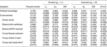


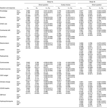


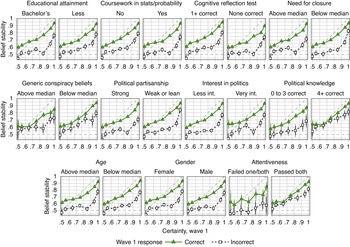




Comments
No Comments have been published for this article.