Nomenclature
-
 ${P_s}$
-
static pressure
-
${P_t}$
-
total pressure
-
${T_t}$
-
total temperature
-
${H_p}$
-
pressure altitude
-
$Ma$
-
Mach number
-
${T_s}$
-
static temperature
-
$Q$
-
dynamic pressure
-
${V_i}$
-
indicated airspeed
-
${V_t}$
-
true airspeed
-
$V$
-
true airspeed scalar
-
$u,v,w$
-
true airspeed components along body axes
-
${V_e}$
-
ground velocity vector
-
${V_r}$
-
air velocity vector
-
${V_w}$
-
wind velocity vector
-
$A$
-
acceleration vector
-
$g$
-
gravitational acceleration vector
-
${r_k}$
-
innovation
- INS
-
inertial navigation system
- UKF
-
unscented Kalman filter
- RCTM
-
residual chi-square test method
- AIME
-
autonomous integrity monitoring by extrapolation
- FMD
-
feature mode decomposition
- FIR
-
finite impulse response
- IMF
-
intrinsic mode functions
- CapsNet
-
capsule network
- ECA
-
efficient channel attention
- CNN
-
convolutional neural networks
- FCN
-
fully convolutional network
- TCN
-
temporal convolutional network
- t-SNE
-
t-distributed stochastic neighbor embedding


Greek symbol
-
$\alpha $
-
angle-of-attack
-
$\beta $
-
sideslip angle
-
$\omega $
-
angular velocity vector
-
$\phi ,\theta ,\psi $
-
roll, pitch and yaw angle


1.0 Introduction
An air data system (ADS) consists of multiple sensors and an air data computer (ADC) belonging to the sensors that measure the atmospheric parameters required during flight. These parameters are transmitted to the atmospheric data computer, which derives the critical flight parameters needed for navigation and control [Reference Nebula, Palumbo and Morani1, Reference Wan, Keviczky and Verhaegen2]. As a key component of the navigation system, ADS plays a vital role in ensuring stable and precise flight. With increasing complexity in aircraft operating environments and combat missions, the risk of ADS failures has significantly escalated [Reference Kilic and Unal3, Reference Prabhu and Anitha4]. Since ADS sensors are mounted on the aircraft surface and feature increasingly complex and integrated internal structures, they have become more prone to failures, including even compound faults. Due to the coupling nature of multiple faults, compound faults are more hazardous and harder to diagnose compared to single faults. Conducting fault diagnosis for ADS is crucial for ensuring reliable aircraft operation and holds practical significance for enhancing mission execution capabilities.
The evolution of compound faults is difficult to interpret through causal relationships, and conventional methods struggle to trace faulty components at the data level due to fault coupling. To address this, scholars have conducted in-depth research. Current compound fault diagnosis techniques can be categorised into three main approaches: fault mechanism-based methods, signal processing-based methods and multi-label classification methods [Reference Huang, Xia and Zhang5, Reference Xu, Zhou and Zhao6].
First, fault mechanism-based methods establish correlations between system models and fault mechanisms based on the inherent characteristics of the system, and identify fault occurrences by analysing changes in model parameters. For instance, an adaptive enhanced unscented Kalman filter (UKF) model was developed [Reference Yu, Lu and Wang7], leveraging diagnostic bond graphs in linear fractional transformation form to derive analytical redundancy relationships for electric scooters. The UKF was then used to distinguish fault types and estimate severity, effectively addressing compound fault diagnosis under parameter uncertainty. Piacentino proposed an improved thermoeconomic method for air conditioning unit faults, analysing variable changes under different faults to create graphical/tabular representations of component interactions, and the method was validated for compound fault scenarios [Reference Piacentino and Talamo8]. Zhang et al. established a four degrees-of-freedom (4-DOF) dynamic model for bearings based on time-varying displacement characteristics, studying vibration patterns under single and compound faults to achieve diagnosis via vibration responses [Reference Zhang, Yan and Liu9]. While these methods offer intuitive and explainable processes, they face challenges such as complex model construction, scalability issues due to diverse fault scenarios and poor adaptability across different systems or environments.
Second, with advancements in signal processing, current approaches fall into two categories: signal decomposition and blind source separation (BSS) [Reference Tang, Luo and Zhang10, Reference Wang, Li and Tang11]. Signal decomposition utilises various analytical methods to decompose signals into different frequency components or modal functions. Different faults exhibit distinct characteristics in these components, enabling the identification of all individual fault features within compound fault signals. Li et al. improved symmetric geometric mode decomposition (SGMD) by employing a morphological envelope cyclic bispectrum to cluster initial components obtained from SGMD decomposition [Reference Li, Jiang and Zhang12]. This approach adaptively separates different fault features contained in compound fault signals while enhancing periodic fault impulses. Subsequently, envelope demodulation was applied to extract fault characteristic frequencies, enabling the diagnosis of gearbox compound faults in strong noise environments. Blind source separation primarily aims to recover original independent source signals from mixed signals, focusing on the statistical independence between sources without prior knowledge of their characteristics or statistical information. To address underdetermined problems caused by insufficient sensors, Hao et al. adopted the sparse component analysis (SCA) algorithm to obtain sparse signal observations [Reference Hao, Song and Ke13]. They first estimated the number of source signals and mixing matrix using potential functions, then achieved source separation through the shortest path method. Experimental validation demonstrated the algorithm’s effectiveness in diagnosing bearing compound faults. Signal processing-based methods can decompose compound faults directly from sensor signals without requiring system modeling. However, these approaches rely on advanced signal processing techniques and specialised expertise and may encounter challenges in ensuring effective decomposition when dealing with compound faults in complex equipment.
Third, unlike single-label classification, multi-label approaches map fault features to multiple fault types via machine learning. Current strategies include problem transformation and algorithm adaptation [Reference Chu, Li and Yang14, Reference Wang, Xu and Zhou15]. Problem transformation converts multi-label tasks into multiple single-label classifications. Wu et al. combined classifier chains with random forests, using prior label predictions as input features to capture label correlations, achieving high accuracy in air-handling unit compound faults [Reference Wu, Cai and Chen16]. Other methods like label power sets [Reference Georgoulas, Climente-Alarcon and Antonino-Daviu17] and random label subsets [Reference Li, Zhou and Qin18] have also shown promise. Algorithm adaptation extends single-label algorithms, such as multi-label K-nearest neighbour (ML-KNN) [Reference Wang, Liu and Deng19, Reference Wang, Liu and Deng20], where the label information of neighbouring instances is determined according to the maximum a posteriori (MAP) principle, and the likelihood of a label is then predicted by statistically analysing the probability of each label’s occurrence among the k-nearest neighbours. With advancements in neural network technology, deep learning algorithms based on multi-label classifiers have been widely applied to the diagnosis of compound faults. Liang et al. designed a wavelet convolutional neural network (CNN)with multi-label encoding and modified activation functions to diagnose variable-speed gearbox compound faults [Reference Liang, Deng and Wu21]. Multi-label classification methods can autonomously extract features of compound faults directly from the data. When the network architecture is well-designed, these methods enable accurate fault localisation even with limited or no compound fault samples, making the design of network structures a key focus of current research. However, this approach relies heavily on the quality and quantity of single-fault samples and still faces limitations inherent to data-driven methodologies.
To conclude, the three mainstream methods each have strengths and limitations in addressing model complexity, data requirements and real-time accuracy. Therefore, it is feasible to consider integrating multiple methods to fully leverage their respective advantages and enhance the diagnostic capability for compound faults. This paper proposes a fault diagnosis method based on UKF and capsule networks (CapsNets) for aircraft ADS. The compound faults considered in this paper include: compound faults between a static pressure system and a total temperature probe, compound faults between the static pressure system and an angle-of-attack sensor, compound faults between a total temperature probe and the sideslip angle sensor and compound faults between the angle-of-attack sensor and the sideslip angle sensor. Building upon the established UKF model of the air data system, feature mode decomposition (FMD) and CapsNets are employed to achieve compound fault location. In our work compared with CNN, fully convolutional network (FCN), temporal convolutional network (TCN), Inception V3 and CapsNet, improved CapsNet do the best for compound fault diagnosis. The main contributions are as follows:
-
(1) Combining UKF with neural networks: A UKF model of ADS was constructed based on the principles of ADS and neural networks to address the issue of fault diagnosis. This integration of UKF and neural networks for ADS fault diagnosis is a novel approach, as existing literature has primarily explored UKF or neural networks independently in fault diagnosis tasks (e.g. Ref. (Reference Sadhukhan, Mitra and Naskar22) for UKF applications; Ref. (Reference Sabour, Frosst and Hinton23) for neural network-based diagnosis), but no prior work has combined these components for ADS compound fault diagnosis.
-
(2) Feature enhancement: The FMD algorithm was employed to enhance fault features [Reference Miao, Zhang and Li24]. Each intrinsic mode function (IMF) component underwent mutual information entropy screening and wavelet threshold denoising before being reconstructed into fault-enhanced sequences, thereby improving the algorithm’s robustness.
-
(3) Hybrid network design: By integrating model data with neural networks, data that effectively reflects fault conditions from the model was selected. After FMD processing, these were input into an improved CapsNet architecture. Combined with the dynamic routing mechanism of CapsNets and a multi-label classifier, this approach achieved accurate compound fault location.
The main structure of this paper is as follows:
-
Section 1 introduces the research background and significance of this study. It surveys the general methods used for fault diagnosis, especially focusing on the current research status of composite fault diagnosis. It also summarises the contributions of this paper and the overall structure of the article.
-
Section 2 introduces the main components of the missile air data system, including the static pressure system, total temperature probe, angle-of-attack sensor, sideslip angle sensor and ADC. It establishes an overall mathematical model and analyses its typical fault mechanisms and models, providing a foundation for subsequent research on fault diagnosis algorithms.
-
Section 3 establishes the UKF dynamic model for ADS and enhances fault features using the FMD method through its output fault information. The processed data is input into the improved CapsNet model, ultimately completing the design of the aircraft ADS composite fault diagnosis algorithm.
-
Section 4 conducts corresponding experimental validation based on the algorithms discussed in previous chapters. By comparing with CNN, FCN, TCN, Inception V3 and CapsNet, it is confirmed that the improved CapsNet used in this paper achieves the best results for composite fault diagnosis.
-
Section 5 summarises the content of this paper and points out some weaknesses of the methods used. It also outlines the key focuses for future research work.
2.0 Air data system modeling and problem formulation
2.1 Air data system modeling
The ADS primarily consists of two components: sensors mounted on the aircraft body surface and an ADC that utilises measurements from these sensors to compute atmospheric flight parameters for the aircraft, as illustrated in Fig. 1.
Schematic diagram of ADS structure.

Based on the interrelationships among the parameters of ADS and using the international standard atmosphere as a reference, the following calculation models can be derived [Reference Sun, Mu and Yao25–Reference Mandle27]:
-
(1) Pressure altitude calculation model
Pressure altitude is directly related to atmospheric pressure. However, under different altitude conditions, influenced by variations in atmospheric temperature and characteristics of air layers, the relationship between pressure and pressure altitude changes accordingly. The specific calculation model is:
 \begin{align}{H_p} = - 46330.7692308\left( {{{\left( {\frac{{{P_s}}}{{127.774}}} \right)}^{0.1902630258}} - 1} \right) - 2000\end{align}
where
 ${H_p}$
is pressure altitude and
 ${P_s}$
is static pressure.
-
(2) Mach number calculation model
The Mach number, defined as the ratio of an aircraft’s true airspeed to the local speed of sound, critically impacts aerodynamic performance, structural design, material selection and flight safety. As the Mach number increases, aerodynamic heating raises the aircraft’s surface temperature. When approaching or exceeding the speed of sound, aerodynamic characteristics undergo significant changes, leading to adverse effects such as shock waves and intense noise. Thus, the Mach number cannot be simply derived by dividing airspeed by the speed of sound but is directly related to atmospheric pressure:
 \begin{align}\frac{{{P_t}}}{{{P_s}}} = {( {1 + 0.2M{a^2}} )^{\frac{K}{{K - 1}}}}\end{align}
Here,
 ${P_t}$
represents total pressure,
 ${P_s}$
represents static pressure,
 $Ma$
represents Mach number, and
 $K$
represents the air adiabatic coefficient. Typically, the adiabatic coefficient
 $K$
is taken as 1.4. Therefore, the formula for calculating Mach number is:
 \begin{align}Ma = \sqrt {5\left( {{{\left( {\frac{{{P_t}}}{{{P_s}}}} \right)}^{\frac{2}{7}}} - 1} \right)} \end{align}
where
 ${P_t}$
is total pressure,
 $Ma$
is the Mach number.
-
(3) Static temperature calculation model
Static temperature plays a pivotal role in evaluating aircraft aerodynamic performance, influencing metrics such as lift, thrust, climb rate and corrections for other parameters. Since temperature probes only measure total temperature, static temperature can be calculated as follows:
 \begin{align}{T_s} = \frac{{{T_t}}}{{1 + 0.2M{a^2}}}\end{align}
where
 ${T_s}$
is static temperature,
 ${T_t}$
is total temperature.
-
(4) Indicated airspeed calculation model
Indicated airspeed reflects the aircraft’s speed relative to the surrounding air, measured directly by the pitot-static system and not corrected for variations in atmospheric pressure or temperature with altitude correlates directly with dynamic pressure and serves as the displayed value on airspeed indicators, representing aerodynamic performance under specific conditions. Combining the Mach number formula with the international standard speed of sound equation, the indicated airspeed equation becomes:
 \begin{align}{V_i} = 1225.44\sqrt {5\left[ {{{\left( {1 + \frac{{\rm{Q}}}{{101.325}}} \right)}^{0.2857}} - 1} \right]} \end{align}
where
 ${V_i}$
is the indicated airspeed,
 $Q$
is dynamic pressure.
-
(5) True airspeed calculation model
True airspeed represents the aircraft’s actual velocity relative to air. Correcting indicated airspeed for altitude and temperature variations (due to air density changes) is crucial for high-altitude flight operations. The calculation formula is:
 \begin{align}{V_t} = 0.35164{V_i}\sqrt {\frac{{{T_s}}}{{{P_s}}}} \end{align}
where
 ${V_t}$
is true airspeed.
The summary of calculation formulas is as follows:
 \begin{align}\left\{ \begin{array}{l}{H_p} = - 46330.7692308\left( {{{\left( {\dfrac{{{P_s}}}{{127.774}}} \right)}^{0.1902630258}} - 1} \right) - 2000\\[15pt]Ma = \sqrt {5\left( {{{\left( {\frac{{{P_t}}}{{{P_s}}}} \right)}^{\frac{2}{7}}} - 1} \right)} \\[8pt]{T_s} = \dfrac{{{T_t}}}{{1 + 0.2M{a^2}}}\\[8pt]{Q_p} = {P_t} - {P_s}\\[4pt]{V_i} = 1225.44\sqrt {5\left[ {{{\left( {1 + \frac{{{{\rm{Q}}_p}}}{{101.325}}} \right)}^{0.2857}} - 1} \right]} \\[10pt]{V_t} = 0.35164{V_i}\sqrt {\dfrac{{{T_s}}}{{{P_s}}}} \end{array} \right.\end{align}
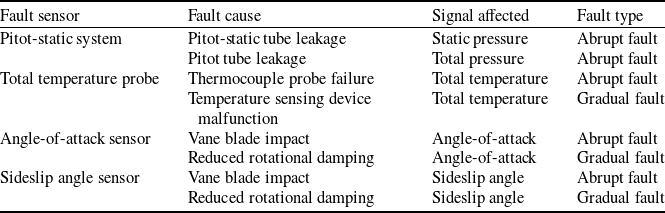
During the flight of an aircraft, the sensors of the air data system located on the surface of the aircraft body are highly susceptible to harsh environmental conditions. This exposure can lead to various types and degrees of malfunctions, posing significant challenges to the reliability of the aircraft’s flight. Based on literature research [Reference Sun and Gebre-Egziabher28–Reference Ossmann31], the typical fault types of the air data system can be summarised as shown in Table 1.
Typical fault of aircraft air data system

Table 1. Long description
A table summarizing typical faults of aircraft air data system sensors. The table has four columns: Fault sensor, Fault cause, Signal affected, and Fault type. It contains seven rows with the following data: Row 1: Fault sensor, Pitot-static system; Fault cause, Pitot-static tube leakage; Signal affected, Static pressure; Fault type, Abrupt fault. Row 2: Fault sensor, Pitot-static system; Fault cause, Pitot tube leakage; Signal affected, Total pressure; Fault type, Abrupt fault. Row 3: Fault sensor, Total temperature probe; Fault cause, Thermocouple probe failure; Signal affected, Total temperature; Fault type, Abrupt fault. Row 4: Fault sensor, Total temperature probe; Fault cause, Temperature sensing device malfunction; Signal affected, Total temperature; Fault type, Gradual fault. Row 5: Fault sensor, Angle-of-attack sensor; Fault cause, Vane blade impact; Signal affected, Angle-of-attack; Fault type, Abrupt fault. Row 6: Fault sensor, Angle-of-attack sensor; Fault cause, Reduced rotational damping; Signal affected, Angle-of-attack; Fault type, Gradual fault. Row 7: Fault sensor, Sideslip angle sensor; Fault cause, Vane blade impact; Signal affected, Sideslip angle; Fault type, Abrupt fault. Row 8: Fault sensor, Sideslip angle sensor; Fault cause, Reduced rotational damping; Signal affected, Sideslip angle; Fault type, Gradual fault.
2.2 Problem formulation
The air data system of an aircraft contains multiple components. After detecting a fault, it is crucial to promptly and accurately locate the source of the failure to facilitate subsequent fault-tolerant control and maintenance. When considering fault types, in addition to individual component failures, compound faults involving simultaneous failures of multiple components represent a significant concern that cannot be overlooked, which further exacerbates the complexity of fault scenarios, making fault location particularly challenging. Currently, the compound fault diagnosis in ADS faces the following primary issues:
-
(1) The aircraft’s ADS comprises multiple sensors, making it difficult to establish a unified model and select key parameters that comprehensively describe the system’s overall characteristics. This poses challenges for implementing effective fault diagnosis based on such models.
-
(2) The complex and variable flight environment of aircraft means that fault information is often obscured by significant noise interference, making fault feature extraction difficult. Effectively processing collected data to enhance fault characteristics remains a critical challenge in compound fault diagnosis.
-
(3) While neural networks can achieve fault location through data, they require substantial data support. However, compound fault data is typically scarce, making it difficult to ensure effective fault location. Exploring methods that leverage mechanistic models without requiring compound fault samples represents another urgent problem to be addressed.
3.0 Fault diagnosis method for aircraft ADS based on UKF and CapsNet
This paper addresses the fault diagnosis problem of aircraft ADS discussed in the previous section by proposing a fault diagnosis method for aircraft ADS based on UKF and CapsNet. The method first correlates sensor measurement parameters through airspeed, angle-of-attack and sideslip angle, establishing the UKF model for atmospheric parameters based on aircraft kinematic equations. Subsequently, feature mode decomposition is employed to enhance fault characteristics in both the extracted model innovations and measurement data, which are then fed as inputs to the neural network. To resolve the decoupling challenge of compound faults, an improved CapsNet is developed: the InceptionV3 network replaces the convolutional layers of the original CapsNet to achieve multi-scale feature extraction, while a multi-label classifier is designed to implement compound fault location. The specific algorithm flow is illustrated in Fig. 2.
Fault diagnosis flowchart.

Figure 2. Long description
A flowchart depicting the process of fault diagnosis. The flowchart is divided into several sections: Model Establishment, Feature Enhancement, and Fault Location. Model Establishment includes an Atmospheric parameters model and a UKF model. The Atmospheric parameters model contains equations for various parameters. The UKF model shows sigma points, UT means, and UT variance. Feature Enhancement includes Feature Mode Decomposition and Mutual information entropy selection, leading to Wavelet threshold denoising and Sequence reconstruction. Fault Location involves an Improved CapsNet with a multi-label classifier, resulting in compound fault location results.
3.1 Kinematic model of ADS
Based on the introduction to the principle of ADS in Section 2.1, among the finally measured parameters, the angle-of-attack and sideslip angle are relatively independent and do not have direct coupling relationships with other parameters. In contrast, true airspeed is directly related to static pressure, total pressure, total temperature and so on. Faults in these parameters can all be reflected through true airspeed. Therefore, the angle-of-attack, sideslip angle and true airspeed can reflect the entire fault condition of the aircraft’s ADS. Coincidentally, these three parameters can also be related through analytical expressions. Starting from this idea, a model for fault diagnosis of ADS can be established.
The angle-of-attack
 $\alpha $
, sideslip angle
 $\beta $
, true airspeed scalar
 $V$
and the components of true airspeed along each axis in the body frame
 ${[ {u,v,w} ]^T}$
are related as follows:
 \begin{align}\left\{ \begin{array}{l}\mathop V\limits^ \bullet = \mathop u\limits^ \bullet \cos \alpha \cos \beta + \mathop v\limits^ \bullet \sin \beta + \mathop w\limits^ \bullet \sin \alpha \cos \beta \\[6pt]\mathop \alpha \limits^ \bullet = - \dfrac{1}{{V\cos \beta }}( {\mathop u\limits^ \bullet \sin \alpha - \mathop w\limits^ \bullet \cos \alpha } )\\[6pt]\mathop \beta \limits^ \bullet = - \dfrac{1}{V}( {\mathop u\limits^ \bullet \cos \alpha \sin \beta - \mathop v\limits^ \bullet \cos \beta + \mathop w\limits^ \bullet \sin \alpha \sin \beta } )\end{array} \right.\end{align}
The dynamics equation of the aircraft in the body frame can be written in the following form:
 \begin{align}\mathop {{V_e}}\limits^ \bullet = A + {T_{be}}g - \omega \times {V_e}\end{align}
where
 ${V_e}$
is the ground velocity vector,
 $A$
is the acceleration vector,
 ${T_{be}}$
is the transformation matrix from the inertial frame to the body frame,
 $g = {\left[ {0,0,9.81} \right]^T}$
, and
 $\omega $
is the angular velocity vector.
According to
 ${V_e} = {V_r} + {V_w}$
, where
 ${V_r}$
is the air velocity vector and
 ${V_w}$
is the wind velocity vector, the equation can be rewritten as follows:
 \begin{align}\mathop {{V_r}}\limits^ \bullet = A + {T_{eb}}g - \omega \times {V_r} - \mathop {{V_w}}\limits^ \bullet - \omega \times {V_w}\end{align}
As the wind velocity is relatively small during aircraft flight, we can denote the wind-related disturbance as
 $d$
,
 $d = - \mathop {{V_w}}\limits^ \bullet - \omega \times {V_w}$
, then define
 ${V_r} = {\left[ {u,v,w} \right]^T}$
,
 $A = {[ {{A_x},{A_y},{A_z}} ]^T}$
,
 $\omega = {[ {p,q,r} ]^T}$
,
 $d = {\left[ {{d_u},{d_v},{d_w}} \right]^T}$
, by substituting Equation (10) into Equation (8), it can be obtained that:
 \begin{align}\left\{ \begin{array}{l}\dot V = \left( {{A_x} - g\sin \theta + {d_u}} \right)\cos \alpha \cos \beta + \left( {{A_y} + g\sin \phi \cos \theta + {d_v}} \right)\sin \beta \\[4pt]\qquad + \left( {{A_z} + g\cos \phi \cos \theta + {d_w}} \right)\sin \alpha \cos \beta \\[4pt]\dot \alpha = [\left( {{A_z} + g\cos \phi \cos \theta + {d_w}} \right)\cos \alpha - \left( {{A_x} - g\sin \theta + {d_u}} \right)\sin \alpha ]/V\cos \beta \\[4pt]\qquad + q - (p\cos \alpha + r\sin \alpha )\tan \beta \\[4pt]\dot \beta = [ - \left( {{A_x} - g\sin \theta + {d_u}} \right)\cos \alpha \sin \beta + ( {{A_y} + g\sin \phi \cos \theta + {d_v}} )\cos \beta \\[4pt]\qquad - \left( {{A_z} + g\cos \phi \cos \theta + {d_w}} \right)\sin \alpha \sin \beta ]/V + p\sin \alpha - r\cos \alpha \end{array} \right.\end{align}
where
 $\phi ,\theta ,\psi $
and represent the roll, pitch and yaw angle, respectively. The estimated attitude angles can be obtained through the following set of motion equations:
 \begin{align}\left\{ \begin{array}{l}\dot \phi = p + q\sin \phi \tan \theta + r\cos \phi \tan \theta \\[4pt]\dot \theta = q\cos \phi - r\sin \phi \\[4pt]\dot \psi = q\dfrac{{\sin \phi }}{{\cos \theta }} + r\dfrac{{\cos \phi }}{{\cos \theta }}\end{array} \right.\end{align}
The combination of Equation (11) and Equation (12) forms the model for the ADS. The sensors of ADS measure the angle-of-attack, sideslip angle and airspeed, and the acceleration and angular velocity can be obtained through the inertial navigation system.
As the ADS exhibits strong nonlinearity, real-time state estimation is performed by the UKF [Reference Sadhukhan, Mitra and Naskar22, Reference Zhang, Guo and Zhang32]. Let the state vector be represented as
 $x = {\left[ {V,\alpha ,\beta ,\phi ,\theta ,\psi } \right]^T}$
. Considering the measurement noise of the inertial navigation system (INS), that of three-dimensional acceleration and angular velocity are denoted as
 $w$
. Therefore, the input vector is represented as
 $u = {[ {{A_{xm}},{A_{ym}},{A_{zm}},{p_m},{q_m},{r_m}} ]^T}$
,
 $u = {[ {{A_x},{A_y},{A_z},p,q,r} ]^T} + w$
. The vertical concatenation of Equations (10) and (11) is
 $f\left( {x,u} \right)$
:
 \begin{align}\mathop x\limits^ \bullet = f\left( {x,u} \right) + G\left( x \right)w + E\left( x \right)d\end{align}
where the disturbance vector
 $d = {\left[ {{d_u},{d_v},{d_w}} \right]^T}$
, and noise matrix
 $G\left( x \right)$
and disturbance matrix
 $E\left( x \right)$
can be respectively represented as follows:
 \begin{align}G\left( x \right) = \left[ {\begin{array}{c@{\quad}c@{\quad}c@{\quad}c@{\quad}c@{\quad}c}{ - \cos \alpha \cos \beta } {}&{ - \sin \beta } {}&{ - \sin \alpha \cos \beta }& {}0 {}&0 {}&0\\[5pt]{\dfrac{{\sin \alpha }}{{V\cos \beta }}} {}&0 {}&{ - \dfrac{{\cos \alpha }}{{V\cos \beta }}} {}&{\cos \alpha \tan \beta } {}&{ - 1} {}&{\sin \alpha \tan \beta }\\[8pt]{\dfrac{{\cos \alpha \sin \beta }}{V}} {}&{ - \dfrac{{\cos \beta }}{V}} {}&{\dfrac{{\sin \alpha \sin \beta }}{V}} {}&{ - \sin \alpha } {}&0 {}&{\cos \alpha }\\[5pt]0 {}&0 {}&0 {}&{ - 1} {}&{ - \sin \phi \tan \theta } {}&{ - \cos \phi \tan \theta }\\[5pt]0 {}&0 {}&0 {}&0 {}&{ - \cos \phi } {}&{\sin \phi }\\[5pt]0 {}&0 {}&0 {}&0 {}&{ - \dfrac{{\sin \phi }}{{\cos \theta }}} {}&{ - \dfrac{{\cos \phi }}{{\cos \theta }}}\end{array}} \right]\end{align}
 \begin{align}E\left( x \right) = \left[ {\begin{array}{c@{\quad}c@{\quad}c}{\cos \alpha \cos \beta } {}&{\sin \beta } {}&{\sin \alpha \cos \beta }\\[5pt]{ - \dfrac{{\sin \alpha }}{{V\cos \beta }}} {}&0 {}&{\dfrac{{\cos \alpha }}{{V\cos \beta }}}\\[8pt]{ - \dfrac{{\cos \alpha \sin \beta }}{V}} {}&{\dfrac{{\cos \beta }}{V}} {}&{ - \dfrac{{\sin \alpha \sin \beta }}{V}}\\[8pt]0 {}&0 {}&0\\ 0 {}&0 {}&0\\0 {}&0 {}&0\end{array}} \right]\end{align}
The measurement equation of the system is:
 \begin{align}z = hx + v\end{align}
where the measurement vector
 $z = {\left[ {{V_m},{\alpha _m},{\beta _m},{\phi _m},{\theta _m},{\psi _m}} \right]^T}$
,
 $v$
represents the corresponding measurement noise,
 $h = {I_{6 \times 6}}$
. To conclude, the state equation and measurement equation of the ADS model are as follows:
 \begin{align}\left\{ \begin{array}{l}\mathop x\limits^ \bullet = f\left( {x,u} \right) + G( x )w + E( x )d\\[3pt]z = hx + v\end{array} \right.\end{align}
3.2 Fault feature selection
Based on the previous analysis of parameter relationships, true airspeed, angle-of-attack and sideslip angle can reflect the fault conditions of sensors in the ADS. Therefore, after establishing a Kalman filter model around these parameters, fault detection can be achieved through methods such as the residual chi-square test method (RCTM) [Reference Wang, Xiong and Liu33, Reference Yun, Kang and Park34]. However, fault location remains challenging using this approach. Herein, by combining data-driven strategies and extracting fault information from model calculations, neural networks’ powerful feature extraction and classification capabilities are utilised to achieve compound fault diagnosis.
According to the RCTM, the innovation vector
 ${r_k}$
which reflects fault information is calculated from the actual measured values
 ${z_k}$
and predicted measurement values
 ${\hat z_{k/k - 1}}$
:
 \begin{align}{r_k} = {z_k} - {\hat z_{k/k - 1}}\end{align}
However, it performs poorly in detecting gradual faults. This is because gradual faults cause only minor changes in the output at any given moment, resulting in small variations in the innovation. Furthermore, the faulty output further affects the estimated value at the next time step, keeping the innovation within a small range and hard to diagnose.
Therefore, the idea of the autonomous integrity monitoring by extrapolation method (AIME) [Reference Yu, Zhang and Zhang35, Reference Liu, Zheng and Wang36] is adopted here, which defines a window of length
 $m$
, starting from steps before a specific point, state estimation is performed and extrapolated to the current time step using the state equation, then the measurement residual at the current time step is calculated. For the time step
 $k$
, assuming that no fault occurred in the system at the time step
 $k - m$
, the state estimate at the time step
 $k$
is extrapolated from the state estimate at the time step
 $k - m$
using the state equation
 $f$
:
 \begin{align}{\hat x_k} = \prod\limits_{i = 1}^m {{f_{\left( i \right)}}} {\hat x_{k - m}}\end{align}
During this process, for each time step from
 $k - m$
to
 $k$
, a corresponding innovation is generated. Specifically, the state estimate
 ${\hat x_{k - m + i}}$
is substituted into the measurement equation to obtain the predicted measurement value at that time step
 $k - m + i$
. This predicted value is then compared with the actual measurement value at the current time step to compute the innovation
 $r_k^{'}$
, then adopting its covariance matrix
 ${V_k}$
. Finally, the average innovation
 ${r_{avg}}$
and the average innovation covariance matrix
 ${V_{avg}}$
within the window can be computed as follows:
 \begin{align}V_{avg}^{ - 1} = \frac{1}{m}\sum\limits_{i = 1}^m {V_k^{ - 1}} \end{align}
 \begin{align}{r_{avg}} = \frac{1}{m}{\left( {V_{avg}^{ - 1}} \right)^{ - 1}}\sum\limits_{i = 1}^m {\left( {V_k^{ - 1}r_k^{'}} \right)} \end{align}
The RCTM algorithm is suitable for abrupt faults, while the AIME algorithm is more appropriate for gradual faults. Therefore, extracting both the innovation and the average innovation of AIME can simultaneously reflect scenarios of abrupt and gradual faults, which aligns well with the context of this study. According to the state equation and measurement equation, both the innovation and AIME innovation contain 6-dimensional parameters each, totaling 12 dimensions. However, the structure of ADS itself is relatively complex. Faults in angle-of-attack and sideslip angle signals can be directly attributed to their respective sensors. Meanwhile, faults in static pressure, total pressure and total temperature signals can manifest through airspeed measurements, yet diagnosing airspeed faults makes it difficult to trace back to specific sources. Thus, additional parameter variations are required to assist in fault location.
Based on the analysis of ADS principles in Section 2.1, the ADC can also calculate parameters such as pressure altitude, static temperature, indicated airspeed and true airspeed. Mechanistic equations reveal that static pressure variations affect pressure altitude, static temperature, indicated airspeed and true airspeed; total pressure changes influence static temperature, indicated airspeed and true airspeed; and total temperature fluctuations impact static temperature and true airspeed, with distinct patterns under different faults. To address this, abrupt faults are reflected using residual values between the current and previous time steps, while gradual faults are identified via the Hurst exponent [Reference Tzouras, Anagnostopoulos and McCoy37, Reference Molino-Minero-Re, García-Nocetti and Benítez-Pérez38]. Nine parameters are selected: pressure altitude residual
 $\Delta {H_p}$
, static temperature residual
 $\Delta {T_s}$
, indicated airspeed residual
 $\Delta {V_i}$
, true airspeed residual
 $\Delta {V_t}$
, angle-of-attack residual
 $\Delta \alpha $
, sideslip angle residual
 $\Delta \beta $
, and the Hurst exponent of static temperature, angle-of-attack and sideslip angle. These 9-dimensional parameters are combined with the aforementioned 12-dimensional innovations to form a 21-dimensional dataset, which serves as input to the neural network model for compound fault location.
3.3 Fault feature enhancement based on feature mode decomposition
The parameters of the extracted dataset mentioned above essentially represent noise sequences that combine system uncertainty and measurement errors, whose data characteristics are closely related to environmental conditions. Due to the harsh operating environment of aircraft air data systems, excessive noise often overwhelms fault signals. Therefore, it is necessary to enhance fault information to create clearer distinctions between normal and fault states.
FMD is currently the latest modal decomposition method specifically designed for mechanical fault diagnosis [Reference Yan and Jia39]. It employs adaptive finite impulse response (FIR) filters to decompose different modes and evaluates decomposition effectiveness based on correlated kurtosis. This method accurately extracts fault information with strong applicability in fault diagnosis. The main steps are as follows:
-
(1) Parameter initialisation
Before decomposing the data extracted in Section 3.2, two types of parameters require initialisation: one is the iteration parameters, including the number of modes
 $n$
and filter length
 $L$
. The other is the FIR filter settings, including filter bank count
 $K$
, initial iteration round
 $i$
and maximum iterations
 ${i_{\max }}$
.
-
(2) Mode decomposition
After obtaining results from each FIR filter
 $f_k^i$
, the initially decomposed modes are calculated as:
 \begin{align}u_k^i = x * f_k^i\end{align}
where
 $u_k^i$
represents the decomposed modes,
 $k = 1,2, \cdots ,K$
,
 $x$
is the input parameter sequence, and
 $*$
denotes convolution operation.
-
(3) Cyclic iteration
Estimate the fault period
 $T_k^i$
based on the timing when the autocorrelation spectrum of
 $u_k^i$
reaches its local maximum
 $R_k^i$
after zero-crossing. Update filter coefficients with
 $i = i + 1$
: if
 $i \lt {i_{\max }}$
, proceed to next steps; otherwise, return to Step (2).
-
(4) Calculate correlation coefficients between all decomposed mode pairs:
 \begin{align}{\rho _{pq}} = \frac{{\sum\limits_{n = 1}^N {\left( {{u_p}\left( n \right) - {{\bar u}_p}} \right)\left( {{u_q}\left( n \right) - {{\bar u}_q}} \right)} }}{{\sqrt {{{\sum\limits_{n = 1}^N {\left( {{u_p}\left( n \right) - {{\bar u}_p}} \right)} }^2}} \sqrt {{{\sum\limits_{n = 1}^N {\left( {{u_q}\left( n \right) - {{\bar u}_q}} \right)} }^2}} }}\end{align}
where
 ${\rho _{pq}}$
is the correlation coefficient between modes
 ${u_p}$
and
 ${u_q}$
, with
 ${\bar u_p}$
,
 ${\bar u_q}$
being their respective means. Select the two modes with the highest correlation, compute their correlated kurtosis using
 $T_k^i$
and retain the component with higher kurtosis. Set
 $K = K - 1$
. Repeat until reaching the preset
 $n$
, then output final results.
This decomposition method overcomes limitations of filter shape and bandwidth, enables thorough signal decomposition, mitigates mode mixing under complex noise and demonstrates robustness against interference [Reference Miao, Zhang and Li24].
Each parameter sequence, after being decomposed by FMD, forms several IMF components and a residual component. Among these IMFs, there exist interference signals weakly correlated with the original fault signal. Therefore, screening based on data characteristics is required to highlight fault features hidden within the signal while reducing noise interference. Here, mutual information entropy – an index reflecting the correlation between IMF components – is used to select IMFs that better represent faults, followed by wavelet threshold denoising.
-
(1) Mutual information entropy selection
Mutual information entropy measures the dimensionless statistical quantity that reflects how much information one random variable provides about another. It quantifies the reduction in uncertainty of one variable due to knowledge of the other, representing the amount of information shared between them. Thus, mutual information entropy evaluates the correlation between the original signal and each IMF component: higher mutual information entropy indicates stronger correlation. The number of modes determined earlier may vary with each decomposition iteration. Given the differing characteristics of parameters and the difficulty in setting precise thresholds, the mutual information entropy between each IMF and the original signal is calculated, retaining the five IMFs with the highest mutual information entropy. This approach emphasises fault features and mitigates noise through information relevance. Meanwhile, it eliminates subjective threshold-setting, which fixes data dimensionality and enhances the rationality and usability of decomposition results.
-
(2) Wavelet threshold denoising
After screening IMFs through FMD, residual fluctuations affecting fault diagnosis may persist. To further enhance fault features, denoising can be applied to each IMF. Wavelet threshold denoising – a classical method combined with modal components – leverages wavelet transform’s strong decorrelation capability. Signal energy concentrates in large wavelet coefficients, while noise distributes across the entire wavelet domain. Thus, after wavelet decomposition, signal coefficients exhibit larger magnitudes than noise coefficients [Reference Jing-Yi, Hong and Dong40]. Coefficients below the threshold are discarded as noise, and wavelet reconstruction completes the denoising process.
3.4 Compound fault location based on improved CapsNet
After the data is processed by FMD, the location of compound faults is achieved through the neural network. CapsNet is a deep learning architecture designed to overcome the limitations of traditional neural networks in handling spatial relationships and hierarchical features. Its excellent performance on the overlapping Modified National Institute of Standards and Technology (MNIST) dataset demonstrates significant potential for addressing compound fault diagnosis [Reference Sabour, Frosst and Hinton23], making it suitable for locating compound faults in ADS. Unlike traditional neural networks, CapsNets introduce ‘capsules’ as fundamental units. Each capsule represents an entity with specific features, encapsulating both feature attributes and spatial relationships. The detailed structure is as follows:
-
(1) Encoder
The encoder consists of three parts: convolutional layer, primary capsule layer and digit capsule layer. The convolutional layer uses a large kernel to initially extract features. Since the output of this layer serves as the input for the capsule structure, to enhance the feature extraction capability while reducing model parameters, the InceptionV3 network [Reference Kumar, Ranawat and Kankar41] is used instead of the convolutional layer shown in Fig. 3, combined with the efficient channel attention (ECA) [Reference Wang, Wu and Zhu42], a lightweight attention mechanism, to improve the efficiency of network operations while extracting features at multiple scales.
Structure of InceptionV3 network.

To address the coupling issue of compound faults, a nonlinear mapping relationship is constructed between the primary capsules and higher-level capsules through dynamic routing, which is also the core mechanism of CapsNets. In traditional CNN, max-pooling only retains the largest features, leading to the loss of much detailed information. In CapsNets, the detailed pose information is preserved through capsules, making it more suitable for detecting compound features, as shown in Fig. 4.
Structure of dynamic routing.

If the activation vector and the prediction vector have a high degree of similarity, it indicates a strong correlation between the two capsules. This similarity is measured by the scalar product of the prediction vector and the activation vector, taking into account both the probability and the feature properties, unlike neurons that only consider the probability. Dynamic routing can be seen as a parallel attention mechanism, allowing the model to recognise multiple objects even when they overlap. Therefore, this is also the core mechanism for CapsNets to achieve compound fault diagnosis, making them more suitable for scenarios where multiple faults occur simultaneously.
-
(2) Decoder
In conventional classification tasks, the output of the encoder is the classification result. To further improve the training effect of the model, the CapsNet also includes a decoder, which reconstructs the correct output from the digit capsule layer through three fully connected layers. This allows for the calculation of loss with the original input data, enhancing the interpretability of the model. Thus, the loss function of the CapsNet consists of margin loss and reconstruction loss, using a margin loss function and mean squared error loss function, respectively.
-
(3) Multi-label classifier
For conventional single-label output problems, the Softmax function is generally used as the classification function, meaning that an increase in the probability of one class leads to a corresponding decrease in the probabilities of other classes, making it unsuitable for compound fault diagnosis problems that require the simultaneous output of multiple labels. Therefore, in the multi-label classifier of the CapsNet, the Sigmoid function is used instead of Softmax. After feature extraction by the CapsNet, the probability of one or more fault labels corresponding to the actual fault types will be significantly higher. Thus, a threshold can be set, and if the probability of a certain predicted label or several predicted labels exceeds this threshold, it indicates that the corresponding fault has occurred, thereby achieving the diagnosis of compound faults.
The final structure of the CapsNet is shown in Fig. 5. Here, the InceptionV3 network replaces the convolutional layer, performing feature extraction through four parallel channels, namely, (a) 1 × 1 convolution, (b) 1 × 1 convolution + 1 × 3 convolution + 3 × 1 convolution, (c) 1 × 1 convolution + 1 × 3 convolution + 3 × 1 convolution + 1 × 3 convolution + 3 × 1 convolution, and (d) 3 × 3 max pooling + 1 × 1 convolution and then concatenating the outputs along the channel dimension, followed by the ECA attention mechanism to enhance feature extraction. The primary capsule layer is designed as four parallel convolutional layers, with the outputs concatenated and activated by the Squash activation function. In the digit capsule layer, the weighted activation of capsule vectors is achieved through the dynamic routing mechanism, with the final output vector’s length (L2 norm) representing the probability of the category. The decoder consists of three fully connected layers with ReLU activation functions, reconstructing the input data to form the reconstruction loss, which, together with the margin loss generated by the encoder, constitutes the loss function, with backpropagation of errors during the training of the neural network.
Structure of improved CapsNet.

Figure 5. Long description
A diagram of the structure of an improved capsule network. The diagram includes several labeled components and processes. Input data flows into a convolutional layer, followed by an InceptionV3 module with an efficient channel attention mechanism. The output then passes through a primary capsule layer, a parallel convolution layer, and a squash function. This is followed by a digit capsule layer with dynamic routing and L2 normalization. The output from the digit capsule layer is processed through a sigmoid function and a threshold to produce diagnosis results. Additionally, the output is fed into a decoder consisting of three fully connected layers with ReLU activation functions. The decoder’s output is used to calculate margin loss and reconstruction loss, which contribute to the overall loss. The diagram illustrates the flow and interaction of these components in the improved capsule network.
4. Experimental validation
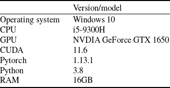
Firstly, a detailed account of the simulation environment is shown in Table 2.
Simulation environment

Table 2. Long description
A table listing specifications for a simulation environment. The table has two columns: one for component labels and one for version or model details. The table has seven rows. Row 1: Operating system, Windows 10. Row 2: CPU, I5-9300H. Row 3: GPU, NVIDIA GeForce GTX 1650. Row 4: CUDA, 11.6. Row 5: Pytorch, 1.13.1. Row 6: Python, 3.8. Row 7: RAM, 16GB.
4.1 Dataset
To verify the applicability of the proposed algorithm, an aircraft system model is built on the Simulink simulation platform. The simulated aircraft flies at subsonic speed, with an airframe mass of 852 kg and fuel mass of 300 kg. To match real-world flight scenarios during the flight, the atmospheric model in the UAV flight system adopts the 1976 International Standard Atmosphere Model, the gravity model uses the gravity calculation model from the World Geodetic System, and the environmental wind adopts the Dryden turbulence model. This model consists of six modules, including the dynamics and kinematics, engine, rudder loop, control system, navigation system and guidance system. The navigation system includes an inertial navigation system/Global Positioning System (INS/GPS) and air data system, with the UKF model embedded in the ADS section. The total flight time is set to 50 s, with faults randomly injected between 25 s and 40 s. The simulation platform has a sampling frequency of 100 Hz, meaning data points are generated every 0.01 s.
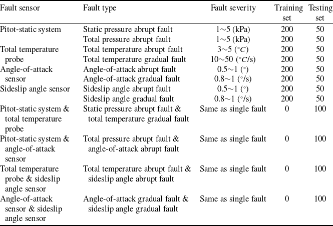
Throughout the network training process, the training set consists of data from four single-fault scenarios in ADS, while the testing set contains both single-fault and compound-fault scenarios. Considering practical scenarios, this study does not consider situations where three or more faults occur simultaneously. Based on the working mechanisms of components in ADS, the angle-of-attack sensor and sideslip angle sensor share similar operational principles, making them prone to compound faults; other fault types need only combine with either of these two sensors to demonstrate compound fault characteristics. Therefore, the compound faults considered in this chapter include: (1) compound faults between static pressure system and total temperature probe, (2) compound faults between static pressure system and angle-of-attack sensor, (3) compound faults between total temperature probe and sideslip angle sensor, and (4) compound faults between angle-of-attack sensor and sideslip angle sensor. These configurations encompass combinations of abrupt faults and gradual faults. Specific parameter settings are detailed in Table 3.
Fault setting table

Table 3. Long description
The table has six columns: Fault sensor, Fault type, Fault severity, Training set, and Testing set. It contains data for various fault scenarios in an aircraft data system. The table includes information on single and compound faults for different sensors, specifying the fault type, severity, and the number of instances used in the training and testing sets. The sensors listed are the Pitot-static system, Total temperature probe, Angle-of-attack sensor, and Sideslip angle sensor. The table also includes compound faults involving combinations of these sensors. Each row provides specific details for a particular fault scenario. Row 1: Pitot-static system, Static pressure abrupt fault, 1-5 kPa, 200, 50. Row 2: Pitot-static system, Total pressure abrupt fault, 1-5 kPa, 200, 50. Row 3: Total temperature probe, Total temperature abrupt fault, 3-5 degrees Celsius, 200, 50. Row 4: Total temperature probe, Total temperature gradual fault, 10-50 degrees Celsius per second, 200, 50. Row 5: Angle-of-attack sensor, Angle-of-attack abrupt fault, 0.5-1 degree, 200, 50. Row 6: Angle-of-attack sensor, Angle-of-attack gradual fault, 0.8-1 degree per second, 200, 50. Row 7: Sideslip angle sensor, Sideslip angle abrupt fault, 0.5-1 degree, 200, 50. Row 8: Sideslip angle sensor, Sideslip angle gradual fault, 0.8-1 degree per second, 200, 50. Row 9: Pitot-static system and total temperature probe, Static pressure abrupt fault and total temperature gradual fault, Same as single fault, 0, 100. Row 10: Pitot-static system and angle-of-attack sensor, Total pressure abrupt fault and angle-of-attack abrupt fault, Same as single fault, 0, 100. Row 11: Total temperature probe and sideslip angle sensor, Total temperature abrupt fault and sideslip angle abrupt fault, Same as single fault, 0, 100. Row 12: Angle-of-attack sensor and sideslip angle sensor, Angle-of-attack gradual fault and sideslip angle gradual fault, Same as single fault, 0, 100.
4.2 Parameter settings
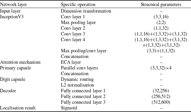
Set the time window length of the data to 50 (0.5 s) and the batch size to 32, resulting in an initial input data dimension of (32, 50, 21). The specific structural parameters of the CapsNet are shown in Table 4.
Network architecture configuration of improved CapsNet

Table 4. Long description
A table detailing the network architecture configuration of an improved CapsNet. The table has three columns: Network layer, Specific operation, and Structural parameters. It contains 14 rows, each describing a different layer or mechanism within the network. Row 1: Input layer, Dimension transformation, blank. Row 2: InceptionV3, Conv layer 1, (3,3,16). Row 3: InceptionV3, Max pooling layer, (2,2). Row 4: InceptionV3, Conv layer 2, (1,1,32). Row 5: InceptionV3, Conv layer 3, (1,1,16)+(1,3,32)+(3,1,32). Row 6: InceptionV3, Conv layer 4, (1,1,16)+(1,3,32)+(3,1,32)+(3,3,32). Row 7: InceptionV3, Max pooling/conv layer, (3,3)+(1,1,32). Row 8: InceptionV3, Concatenation, blank. Row 9: Attention mechanism, ECA layer, blank. Row 10: Primary capsule, Parallel conv layers, (3,3,32)*4. Row 11: Primary capsule, Concatenation, blank. Row 12: Digit capsule, Dynamic routing, blank. Row 13: Digit capsule, L2 normalisation, blank. Row 14: Decoder, Fully connected layer 1, (32,256). Row 15: Decoder, Fully connected layer 2, (256,512). Row 16: Decoder, Fully connected layer 3, (512,600). Row 17: Localisation result, Sigmoid, blank.
All convolutional layers follow the structure of [Conv + BatchNorm + ReLU activation], which accelerates convergence and enhances generalisation. Default configurations: stride=1 and padding=0. The structural parameters are defined as follows: taking ‘(1,1,16)+(1,3,32)+(3,1,32)’ as an example, it represents sequential operations: 1 × 1 convolution (16 channels) → 1 × 3 convolution (32 channels) → 3 × 1 convolution (32 channels).
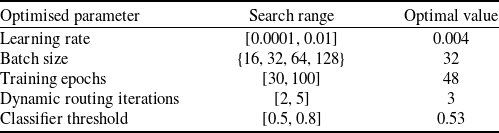
The beluga whale optimisation algorithm was employed to optimise hyperparameters of the CapsNet, including learning rate, batch size, training epochs, dynamic routing iterations and multi-label classifier threshold. The objective function minimises the difference between accuracy and 1. The optimal parameters obtained are shown in Table 5.
Parameter optimisation results

Table 5. Long description
A table showing optimized parameters for a beluga whale optimization algorithm. The table has five rows and three columns. The columns are labeled Optimised parameter, Search range, and Optimal value. Row 1: Optimised parameter, Learning rate; Search range, [0.0001, 0.01]; Optimal value, 0.004. Row 2: Optimised parameter, Batch size; Search range, [16,"32","64", 128]; Optimal value, 32. Row 3: Optimised parameter, Training epochs; Search range, [30, 100]; Optimal value, 48. Row 4: Optimised parameter, Dynamic routing iterations; Search range, [2, 5]; Optimal value, 3. Row 5: Optimised parameter, Classifier threshold; Search range, [0.5, 0.8]; Optimal value, 0.53.", "EDH": "
4.3 Results and analysis
-
(1) Location results of single fault
Since the neural network training dataset contains only single-fault cases without compound faults, the single-fault classification capability of the CapsNet is first verified. The confusion matrix is shown in Fig. 6.
Confusion matrix of improved CapsNet under single fault.

Confusion matrix of CapsNet and InceptionV3 (a) confusion matrix of CapsNet (b) confusion matrix of InceptionV3.

Figure 7. Long description
Panel A: Confusion matrix of CapsNet. This matrix has four rows and four columns, each representing different fault types: P Fault, Tt Fault, alpha Fault, and beta Fault. The diagonal elements show the accuracy of correct predictions, with values close to 1.0 indicating high accuracy. Notable values include 0.9798 for P Fault, 1.000 for Tt Fault, 0.9588 for alpha Fault, and 0.9787 for beta Fault. Off-diagonal elements represent misclassifications, with values generally close to 0.000, indicating low rates of misclassification. Panel B: Confusion matrix of InceptionV3. This matrix also has four rows and four columns, representing the same fault types. The diagonal elements show the accuracy of correct predictions, with values close to 1.0 indicating high accuracy. Notable values include 0.9588 for P Fault, 0.9785 for Tt Fault, 0.9895 for alpha Fault, and 1.000 for beta Fault. Off-diagonal elements represent misclassifications, with values generally close to 0.000, indicating low rates of misclassification.
The figure demonstrates that the main diagonal elements of the confusion matrix all approaching 1, which indicates a classification accuracy nearing 100%, enabling accurate identification of fault conditions in various sensors of ADS, thereby proving the precision of the improved CapsNet in single fault localisation.
To validate the enhancement effect of the proposed network over traditional CapsNets, ablation experiments were conducted by comparing with the following networks: (a) the original CapsNet; (b) the InceptionV3 network. The confusion matrices of these two networks are shown in Fig. 7. Under identical experimental settings, both networks exhibit some decline in localisation performance compared to their combined version. On one hand, the CapsNet preserves feature pose information through capsules and largely retains the dynamic routing mechanism, enabling faster convergence with limited samples compared to InceptionV3. On the other hand, replacing the convolutional layers of the CapsNet with InceptionV3 and integrating the ECA attention mechanism allows multi-scale extraction of fault information during the initial feature extraction phase. Therefore, the improved CapsNet combining both approaches demonstrates superior classification capabilities.
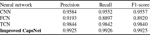
Comparative experiments were conducted with commonly used neural network models in fault diagnosis, including CNN, FCN and TCN. Evaluation metrics such as precision, recall, and F1-score were selected. The models were tested using the same testing set, and the fault diagnosis results are summarised in Table 6.
Statistical table of localisation metrics for different neural networks under single fault

Table 6. Long description
A table comparing the performance metrics of different neural networks under single fault conditions. The table has four rows and four columns. The columns are labeled Neural network, Precision, Recall, and F1-score. The row labels are CNN, FCN, TCN, and Improved CapsNet. Row 1: CNN, Precision 0.9584, Recall 0.9552, F1-score 0.9557. Row 2: FCN, Precision 0.9193, Recall 0.8897, F1-score 0.8920. Row 3: TCN, Precision 0.9844, Recall 0.9842, F1-score 0.9840. Row 4: Improved CapsNet, Precision 0.9925, Recall 0.9926, F1-score 0.9925.
According to the metrics, while some networks like TCN achieved relatively good performance for single-fault scenarios, the improved CapsNet demonstrated higher accuracy overall. Since compound faults are classified based on training results from single-fault data, it is crucial to first ensure the network’s correct identification of individual faults.
Visual analysis of feature classification effectiveness using the t-SNE algorithm is shown in Fig. 8, where label ‘1’ represents pitot-static system fault, label ‘2’ represents total temperature probe fault, label ‘3’ represents angle-of-attack sensor fault and label ‘4’ represents sideslip angle sensor fault. The visualisation reveals that other neural networks exhibit close classification distances for certain fault categories. Although final classification results might appear correct, this proximity makes it difficult to decouple overlapping fault types during subsequent compound fault experiments. In contrast, CapsNet effectively amplifies inter-class differences while minimising intra-class variations, thereby laying a foundation for accurate compound fault location.
-
(2) Location results of compound fault
t-SNE visualisation results of feature extraction for different neural networks (a) CNN (b) FCN (c) TCN (d) InceptionV3 (e) CapsNet (f) improved CapsNet.

Based on the predefined fault types, the training set remained unchanged with only single-fault data, while the testing set included a mixture of single and compound faults. The confusion matrix of the proposed model under this configuration is shown in Fig. 9.
Confusion matrix of improved CapsNet under compound fault.

Figure 9. Long description
A confusion matrix showing the performance of an improved CapsNet under compound fault conditions. The matrix has eight rows and eight columns, each representing different fault types: P Fault, Tt Fault, alpha Fault, beta Fault, P-Tt Fault, P-alpha Fault, Tt-beta Fault, and alpha-beta Fault. The rows are labeled as true labels and the columns as predicted labels. The diagonal elements of the matrix represent the correct classifications, with values close to 1.0 indicating high accuracy. Notable values include 0.9900 for P Fault, 1.000 for Tt Fault, 0.9900 for alpha Fault, 1.000 for beta Fault, 0.9800 for P-Tt Fault, 0.9000 for P-alpha Fault, 0.9300 for Tt-beta Fault, and 0.9000 for alpha-beta Fault. Off-diagonal elements represent misclassifications, with values indicating the proportion of instances where one fault type was predicted as another.
Experimental results indicate that while the classification accuracy for single faults remains high in this mixed testing set, the accuracy for compound faults decreases, particularly for faults involving the angle-of-attack. For instance, concurrent faults in the pitot-static system and angle-of-attack sensor, as well as simultaneous faults in the sideslip angle sensor and angle-of-attack sensor, achieved only 90% correct localisation accuracy, lower than other fault types. This occurs because the angle-of-attack signal measured by the sensor significantly influences control and guidance systems in the aircraft model. When combined with faults from other sensors, the fault features become highly coupled, leading to misclassification between single and compound faults when applying thresholds in the multi-label classifier. Nevertheless, the overall compound fault localisation accuracy remains satisfactory, with all categories achieving above 90% accuracy.
To validate the applicability of the improved CapsNet for compound faults, the proposed model was compared with the original CapsNet architecture and other neural networks. Taking CNN as an example, its confusion matrix is shown in Fig. 10. The results demonstrate that while CNN achieves reasonable accuracy for single-fault localisation, it exhibits almost no capability for compound fault classification. This limitation stems from CNN’s tendency to prioritise dominant features and retain only the highest-probability category information. Although the final output uses Sigmoid activation for multi-label classification, the model often produces outputs where one class approaches 1 while others remain near 0. Consequently, it becomes challenging to set appropriate thresholds to identify secondary fault categories with lower-probability outputs in compound fault scenarios.
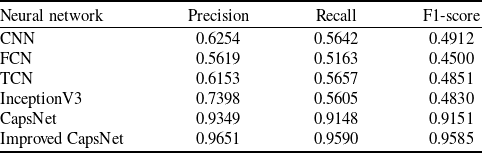
To ensure the reliability of the testing, five-fold cross-validation was employed. The averaged metrics for fault location results are summarised in Table 7, and error bar curves are plotted in Fig. 11.
Based on the experimental results, conventional neural networks, similar to CNN, struggle to classify compound faults. They tend to output only the category with the highest probability, ultimately misclassifying compound faults as single faults. In contrast, the CapsNet leverages dynamic routing between capsules to extract features for each fault category independently. Combined with the Squash activation function and L2 norm, it outputs probabilities for each category, ensuring that the presence of one fault minimally interferes with the identification of others. This design typically results in fault category probabilities exceeding 0.5, simplifying threshold configuration and improving localisation accuracy. Replacing the convolutional layers of the CapsNet with an InceptionV3 + ECA architecture further enhances feature extraction, boosting both the precision and stability of compound fault location.
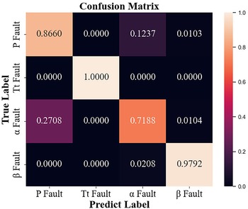
Finally, to validate the necessity of using UKF innovation in the proposed algorithm, a comparison was made with fault location results derived directly from raw sensor measurement signals. The measurement signals included nine parameters: true airspeed, angle-of-attack, sideslip angle, pitch angle, roll angle, yaw angle, pressure altitude, static temperature and indicated airspeed. These parameters align with those used in the proposed method, with the key distinction being whether the data is derived from UKF-modeled innovations or raw measurements. All other fault location procedures remained identical. The confusion matrices based on raw measurement signals are shown in Figs 12 and 13.
Statistical table of localisation metrics for different neural networks under compound fault

Table 7. Long description
A table comparing the performance metrics of different neural networks under compound fault conditions. The table has six rows and four columns. The columns are labeled Neural network, Precision, Recall, and F1-score. The row labels are CNN, FCN, TCN, InceptionV3, CapsNet, and Improved CapsNet. Row 1: CNN, Precision: 0.6254, Recall: 0.5642, F1-score: 0.4912. Row 2: FCN, Precision: 0.5619, Recall: 0.5163, F1-score: 0.4500. Row 3: TCN, Precision: 0.6153, Recall: 0.5657, F1-score: 0.4851. Row 4: InceptionV3, Precision: 0.7398, Recall: 0.5605, F1-score: 0.4830. Row 5: CapsNet, Precision: 0.9349, Recall: 0.9148, F1-score: 0.9151. Row 6: Improved CapsNet, Precision: 0.9651, Recall: 0.9590, F1-score: 0.9585.
Confusion matrix of CNN under compound fault.

Figure 10. Long description
A confusion matrix showing the performance of a convolutional neural network under compound fault conditions. The matrix has eight rows and eight columns, each representing different fault types. The rows are labeled with true labels and the columns with predicted labels. The diagonal elements represent correct predictions, with values close to 1.0 indicating high accuracy. Notable trends include high accuracy for P Fault, Tt Fault, and beta Fault, with values of 0.9600, 0.9900, and 1.0000 respectively. The matrix also shows some misclassifications, such as a 0.3000 value for P-alpha Fault under the true label of P Fault and a 0.5200 value for P-alpha Fault under the true label of Tt-beta Fault. The color scale on the right indicates the probability values, ranging from 0.0 to 1.0.
The confusion matrices reveal that when raw measurement signals are directly used as input to the neural network, the classification performance for both single and compound faults is suboptimal. This occurs because the flight navigation points, speeds and fault injection times in the aircraft scenario are randomised. With limited training data unable to cover all flight states, variations in the data – whether caused by changes in flight settings or faults – become indistinguishable. Consequently, subtle faults are difficult to isolate and localise. In contrast, the innovation sequences calculated by the UKF model fluctuate near zero under normal conditions. When a fault occurs, these sequences exhibit significant deviations from their baseline, making fault features easily extractable and distinguishable. The statistical metrics are summarised in Table 8.
Statistical table of localisation metrics under different fault scenarios and data

Table 8. Long description
A table with four rows and four columns comparing fault scenarios and data types with precision, recall, and F1-score metrics. The columns are labeled Data, Precision, Recall, and F1-score. The rows are labeled Single fault and Compound fault, with two sub-rows each for Measurement signals and UKF innovation. Row 1: Single fault, Measurement signals, Precision 0.8935, Recall 0.8910, F1-score 0.8904. Row 2: Single fault, UKF innovation, Precision 0.9925, Recall 0.9926, F1-score 0.9925. Row 3: Compound fault, Measurement signals, Precision 0.5262, Recall 0.5038, F1-score 0.4533. Row 4: Compound fault, UKF innovation, Precision 0.9651, Recall 0.9590, F1-score 0.9585.
Error bar chart of fault location effectiveness for different neural networks.

Localisation confusion matrix based on measurement signals under single fault.

Localisation confusion matrix based on measurement signals under compound fault.

Figure 13. Long description
A confusion matrix with seven rows and seven columns, comparing true labels and predicted labels for different fault types. The rows represent true labels, and the columns represent predicted labels. The matrix includes values indicating the proportion of correct and incorrect classifications for each fault type. Notable values include high accuracy for Tt Fault and beta Fault, with values of 0.9700 and 0.8600 respectively, and lower accuracy for alpha Fault and P-alpha Fault, with values of 0.4200 and 0.1900 respectively. The matrix uses a color gradient to represent the values, with lighter colors indicating higher values and darker colors indicating lower values.
Since the classification accuracy of single faults directly impacts compound fault location, CapsNet trained on raw measurement signals demonstrates severely degraded compound fault location capabilities, with all metrics hovering around 50% when it fails to accurately identify single faults. This starkly contrasts with the diagnostic results based on UKF-modeled innovations, further validating the superior accuracy of the improved CapsNet when leveraging model innovation for fault location.
5.0 Conclusion
This paper proposes a fault diagnosis method for compound faults in aircraft air data systems based on UKF and CapsNet. The method establishes a UKF model for atmospheric parameters by selecting key variables derived from the principles of ADS and aircraft kinematic equations. To enhance fault feature extraction, feature mode decomposition is applied to refine the innovation sequences generated during UKF computation, which are then fed into the neural network. Additionally, an improved CapsNet is designed, where the convolutional layers are replaced with an InceptionV3 architecture to strengthen feature extraction capabilities, and the multi-label classifier is implemented to enable precise localisation of compound faults. Simulation experiments under single and compound fault scenarios demonstrate that the proposed algorithm achieves robust fault location for aircraft ADS, with accuracy exceeding 95%. This performance significantly outperforms methods relying on raw measurement signals or other neural networks. Future work will focus on extending the algorithm to more complex environmental conditions and fault scenarios, further refining its generalisability and practical engineering value.
However, this research still has certain limitations, and future work can be developed based on these aspects: first, this paper considers several typical representative faults in the ADS. Complex situations such as improper installation and circuit faults cannot be covered by the methods used in this paper. Future research can consider how to incorporate these fault conditions into logical judgement. Second, this paper does not consider the specific degree of fault magnitude. Future research can focus on how to distinguish the specific degree of fault occurrence. Finally, the neural network method based on CapsNets lacks strong interpretability. This opacity makes its results difficult to be fully trusted. Redundant diagnostic schemes may need to be introduced for cross-validation, thereby increasing actual operation and maintenance costs and limiting its application in scenarios requiring high reliability. Future work can conduct in-depth research on model interpretability or integrate logical reasoning with neural networks to improve the reliability of diagnostic results.
Acknowledgements
This research was funded by the National Key Research and Development Program of China (No. 2023YFB3307102) and the National Natural Science Foundation Integration Project (No. U22B6001).
Competing interests
The authors declare none.