1 Introduction
Turbulent flames are associated with acoustic sound radiation (Mahan & Karchmer Reference Mahan and Karchmer1991; Dowling & Mahmoudi Reference Dowling and Mahmoudi2015), which in turn may lead to thermo-acoustic instabilities in many combustion systems with high reflection properties (Candel et al. Reference Candel, Durox, Ducruix, Birbaud, Noiray and Schuller2009). The problem of sound generation in premixed turbulent flames, and its underlying physical mechanisms, has been thoroughly studied using experiments and, more recently, direct numerical simulations (Zhao & Frankel Reference Zhao and Frankel2001; Shalaby, Laverdant & Thévenin Reference Shalaby, Laverdant and Thévenin2009; Swaminathan et al. Reference Swaminathan, Xu, Dowling and Balachandran2011). Theoretical studies of combustion noise indicate that heat-release disturbances constitute the main source of noise radiated by flames (Strahle Reference Strahle1971). In this case, the local sound pressure level is proportional to the rate of change of the volumetric heat-release rate. These findings were validated in experiments for far-field conditions (Hurle et al. Reference Hurle, Price, Sugden and Thomas1968; Kidin et al. Reference Kidin, Librovich, Roberts and Vuillermoz1984). Unfortunately, owing to the low frequencies typically observed in combustion systems, the strict acoustic far-field limit is rarely achieved in practice. Heat-release-rate sound sources based on the local heat-release rate, however, still provide practicable predictions of noise levels at mid-range acoustic distances (Smith & Kilham Reference Smith and Kilham1963; Candel, Durox & Schuller Reference Candel, Durox and Schuller2004).
Based on previous studies, heat-release-rate variations originate from flame surface density fluctuations (Abugov & Obrezkov Reference Abugov and Obrezkov1978; Clavin & Siggia Reference Clavin and Siggia1991) as well as from local changes in the burning rate (Kidin et al. Reference Kidin, Librovich, Roberts and Vuillermoz1984; Talei, Brear & Hawkes Reference Talei, Brear and Hawkes2011). On the one hand, the instantaneous local flame speed depends on the combustible mixture temperature and pressure, on the equivalence ratio of the mixture and on the flame stretch through the tangential strain rate and the local curvature of the flame front (Markstein Reference Markstein1964; Williams Reference Williams1985). On the other hand, flame surface-area variations can stem from fluctuations in the local burning velocity (Birbaud et al. Reference Birbaud, Ducruix, Durox and Candel2008), from local flame instabilities (Matalon & Matkowsky Reference Matalon and Matkowsky1982; Pelce & Clavin Reference Pelce and Clavin1982; Truffaut & Searby Reference Truffaut and Searby1999), or from interactions with hydrodynamic disturbances (Candel & Poinsot Reference Candel and Poinsot1990; Blanchard et al. Reference Blanchard, Schuller, Sipp and Schmid2015; Schlimpert et al. Reference Schlimpert, Hemchandra, Meinke and Schröder2015). As a consequence of the dependences, flame–vortex interactions represent, for instance, a canonical component when modelling turbulent combustion processes (Driscoll Reference Driscoll2008).
Vortices typically cause a roll-up motion of the flame, thus inducing a strong local stretch (Renard et al. Reference Renard, Thévenin, Rolon and Candel2000). This phenomenon can considerably alter the flame structure and sometimes even induce quenching (Katta et al. Reference Katta, Carter, Fiechtner, Roquemore, Gord and Rolon1998). Alternatively, the roll-up can isolate a portion of cold gases; when the fuel pocket is depleted, quenching occurs. This dynamic process corresponds to a two-phase sequence: first, the reactive surface slowly increases due to the roll-up; second, vast portions of flame surface quickly quench, thereby leading to a large-amplitude acoustic pulse (Candel et al. Reference Candel, Durox, Ducruix, Birbaud, Noiray and Schuller2009). More generally, under stationary operating conditions, it is found that mechanisms yielding flame surface destruction produce far more acoustic output than mechanisms associated with flame surface creation (Candel et al. Reference Candel, Durox and Schuller2004). For instance, in flame–flame interactions, flame pinching has been shown to generate two subsequent acoustic pulses: the first one occurs during pinching, the second one at the end of the flame pocket annihilation (Schuller, Durox & Candel Reference Schuller, Durox and Candel2003; Geiser, Schlimpert & Schroeder Reference Geiser, Schlimpert and Schroeder2013). These impulses have been shown to be related to the local acceleration of the flame burning velocity during the final stage of combustion, when the local flame curvature becomes sufficiently large (Talei, Hawkes & Brear Reference Talei, Hawkes and Brear2013). These studies confirmed that this phenomenon is caused by interpenetrating thermal and species-diffusion layers of neighbouring flame elements (Bui, Schröder & Meinke Reference Bui, Schröder and Meinke2006).
Most of these thermo-acoustic phenomena are intrinsically nonlinear and associated with significant flame-front displacements. Nonetheless, a linear approach can provide important insights into noise-generation processes. Such a methodology, for instance, confirmed that local regions characterized by reaction layers with strong curvature as present in the flame tip are responsible for intense noise emission (Blanchard et al. Reference Blanchard, Schuller, Sipp and Schmid2015). Such a linear framework allows to us separate flow perturbations into entropy, vorticity and acoustic waves (Chu & Kovásznay Reference Chu and Kovásznay1958) and thus uncover a mechanistic viewpoint of flame-induced noise generation. Flat flame fronts are known to strongly absorb vorticity waves (Matalon, Cui & Bechtold Reference Matalon, Cui and Bechtold2003). Experimentally, vortices whose width is 10 to 100 times the flame thickness were observed to attenuate due to viscous effects in the internal structure of the flame front (Roberts & Driscoll Reference Roberts and Driscoll1991). This vortex–flame front interaction may subsequently be associated with strong acoustic radiation; its underlying mechanism, however, has not yet been considered as a possible route to noise generation in flames.
In our study, we consider vortices ranging from 100 flame thicknesses to far larger scales. Even though vortex noise is commonly associated with multipolar pressure sources and is therefore rapidly decaying away from its source (Powell Reference Powell1964), its contribution to the overall acoustic radiation may be significant and play an important role in the near field. A local analysis of flame pressure generation, taking into account a full flame structure, is also relevant. To carry out such an analysis, a flame model is required to generate a base flow. We seek to vary the mean stretch of the flame in a controlled manner in order to investigate its role in the noise-generation mechanism. For this reason, an axisymmetric imploding flame, such as studied by Talei et al. (Reference Talei, Brear and Hawkes2011), is considered. In this configuration, and in the absence of mean vorticity sources, the aerodynamic strain rate vanishes. Stretch is directly related to the flame curvature, i.e. to the flame radius, and an accurate estimate of the stretch is readily accessible from the simulation. The objective of this study is to use numerical techniques and linear perturbation analysis, applied to a simplified but relevant combustion model of a radially imploding flame, to examine the influence of the wavenumber of the hydrodynamic disturbances and the local flame-front curvature on the generation of local pressure sources.
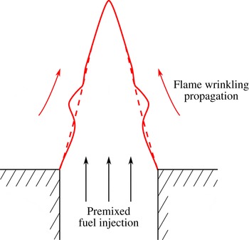
Sketch of a flame-front perturbation propagating along an axisymmetric anchored flame.

2 Configuration, modelling approach and numerical details
Flames submitted to a non-zero tangential velocity tend to propagate wrinkles along the flame front, as sketched in figure 1; this is true even for stable flame configurations (Blackshear Reference Blackshear1953; Petersen & Emmons Reference Petersen and Emmons1961; Boyer & Quinard Reference Boyer and Quinard1990). This well-known behaviour was recently analysed within a linear framework (Blanchard et al. Reference Blanchard, Schuller, Sipp and Schmid2015). Flame perturbations then appear as a superposition of (1) entropy and reaction waves, associated with flame-front displacement, and (2) vorticity waves that enforce mass conservation across the dilatation zone; at the flame tip, this set of waves becomes unstable before it disappears. An analysis of the Lighthill equation for this configuration shows that the associated far-field combustion noise is dominated by the heat-release rate contribution to the acoustics (Lighthill Reference Lighthill1952; Crighton et al. Reference Crighton, Dowling, Ffowcs Williams, Heckl and Leppington1992), and this theoretical result has been confirmed in many experiments (see e.g. Hurle et al. Reference Hurle, Price, Sugden and Thomas1968; Kidin et al. Reference Kidin, Librovich, Roberts and Vuillermoz1984). While these insights are important and consequential for the far field, they provide little understanding of noise-generation mechanisms for the near field. Even though flame wrinkling is an integral component of the flame dynamics, other type of waves may be destabilized by the flame front and lead to localized favourable conditions for high-amplitude noise generation. A local analysis can then provide useful information on these issues. In this study, we will focus on flow structures producing the largest (optimal) acoustic output, without prescribing a specific mechanism for flame-induced noise generation.
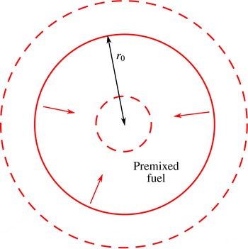
Sketch of an axisymmetric, radially imploding flame.

A simple flame configuration is introduced and used as the basis for our analysis. It consists of a one-dimensional, axisymmetrically imploding cylindrical flame, as shown in figure 2. In this set-up, a flame front propagates towards the centre while burning homogeneously premixed fuel (see e.g. Crighton et al. Reference Crighton, Dowling, Ffowcs Williams, Heckl and Leppington1992; Talei et al. Reference Talei, Brear and Hawkes2011). A fully compressible, reactive Navier–Stokes solver, resolving all spatial and temporal scales, has been used. The reactive component consists of a one-step, one-way chemistry model of Arrhenius type with a local reaction rate of the form
 $$\begin{eqnarray}\displaystyle \dot{{\it\omega}}_{f}=A{\it\rho}Y_{f}T^{{\it\beta}}\exp \!\left(-\frac{T_{a}}{T}\right), & & \displaystyle\end{eqnarray}$$
where
 ${\it\rho}$
is the flow density,
 $Y_{f}$
is the fuel mass fraction,
 $T_{a}$
is the activation temperature and
 $T$
is the local fluid temperature. Coefficients
 $A$
and
 ${\it\beta}$
are kept constant. The time-independent planar flame thickness
 ${\it\delta}_{f}$
is defined in the limit of small local curvature according to (Poinsot & Veynante Reference Poinsot and Veynante2005)
 $$\begin{eqnarray}\displaystyle {\it\delta}_{f}=\frac{T_{b}-T_{u}}{\max |\partial T/\partial r|}, & & \displaystyle\end{eqnarray}$$
with
 $T_{u}$
denoting the temperature of the fresh gases and
 $T_{b}$
the temperature of the burned products. In what follows, the reference length is taken as
 ${\it\delta}_{f}$
, the reference velocity as the laminar burning velocity, and the reference temperature as the temperature of the unburned gases at
 $T_{u}$
. With this choice, we consider the parameters
 $A=6.3\times 10^{10}$
,
 ${\it\beta}=0.35$
and
 $T_{a}=120$
, which yield a reference Reynolds number of
 $Re=5.56$
in fresh gases, a reference Mach number of
 $Ma=0.006$
and a constant Prandtl number of
 $Pr=0.72.$
The heat release of the chemical reaction is set to enforce
 $T_{b}=6.5$
. Differential diffusion is taken into account by Fick’s law at a constant Lewis number
 $Le$
. In what follows, the values
 $Le=0.8$
,
 $1$
and
 $1.2$
will be considered. Finally, the temperature dependence of the viscosity is modelled by Sutherland’s law with
 ${\it\mu}={\it\mu}_{ref}(T/T_{u})^{0.65}$
.
A chemistry model of this type has been used by Williams (Reference Williams1985) to analytically study planar flame fronts. Details about the numerical discretization of our governing equations can be found in Sandberg (Reference Sandberg2007) and Blanchard et al. (Reference Blanchard, Schuller, Sipp and Schmid2015). Our simulations use a conservative formulation of the state variable
 $\boldsymbol{q}=({\it\rho},{\it\rho}u_{r},{\it\rho}u_{{\it\theta}},{\it\rho}E,{\it\rho}Y_{f})^{\text{T}}$
with
 ${\it\rho}$
as the density,
 $(u_{r},u_{{\it\theta}})$
as the radial and angular velocity, respectively,
 $E$
as the total energy and
 $Y_{f}$
as the fuel mass fraction. The computational mesh is adapted to ensure a minimum of
 $25$
grid points across the reaction layer and a proper convergence in the diffusive regions. Absorbing boundary conditions at a large outer radius are employed using a perfectly matched layer along with characteristic boundary conditions (Poinsot & Lele Reference Poinsot and Lele1992).
Our flow analysis consists of a two-step procedure. First, a nonlinear axisymmetric simulation is performed, from which snapshots are extracted at discrete time instants
 $t_{i}$
corresponding to a set of radial positions
 $r_{0}(t_{i})$
that satisfy
 $Y_{f}(r_{0})=0.5$
and
 $0.4\leqslant r_{0}\leqslant 160.$
In a second step, we compute the maximum amount of pressure that can be generated by a linear perturbation superimposed on the extracted flow field at the specific radii. The next section presents more details about this second step.
3 Linear analysis and optimization of acoustic output
The linear operator
 $\unicode[STIX]{x1D63C}$
describing the temporal evolution of perturbations superimposed on a reference state
 $\boldsymbol{q}_{0}$
can formally be defined as
 $\unicode[STIX]{x1D63C}=\partial \boldsymbol{F}(\boldsymbol{q})/\partial \boldsymbol{q}|_{\boldsymbol{q}_{0}}$
, where
 $\boldsymbol{F}$
stands for the nonlinear reactive Navier–Stokes operator and
 $\boldsymbol{q}_{0}$
is taken as the state vector associated with a particular snapshot (Schmid & Henningson Reference Schmid and Henningson2001). Alternatively, the operator
 $\unicode[STIX]{x1D63C}$
is also the rate of change of
 $\boldsymbol{F}$
with respect to
 $\boldsymbol{q}$
, evaluated at
 $\boldsymbol{q}=\boldsymbol{q}_{0}$
.
Our set-up concentrates on perturbations about the nonlinear, non-periodic flow of the imploding flame. Consequently,
 $\boldsymbol{q}_{0}$
changes in time. Because of this fact, choosing the appropriate linear method to investigate this system is not trivial. The time dependence of the base state excludes the direct use of eigenvalues and eigenvectors, without more overly restrictive assumptions of temporal scale separation or limitation to a steady or harmonic base-flow dynamics. The same is true for a frequency response or resolvent analysis, which also requires a time-independent evolution operator
 $\unicode[STIX]{x1D63C}$
. As another option, a direct-adjoint optimization methodology (Schmid Reference Schmid2007; Luchini & Bottaro Reference Luchini and Bottaro2014) could be brought to bear on the problem; this approach introduces a user-specified time horizon over which the acoustic output is optimized and, in addition, requires a computationally involved effort. In our pursuit of an alternative linear analysis technique, we are aided by our focus on acoustic waves generated at the flame front: we can study these waves by concentrating on the time derivative of the pressure, which eliminates the necessity of solving and imposing the time-dependent evolution equation. This approach is equivalent to considering the limit
 $t_{0}\rightarrow 0$
and can be motivated by physical arguments.
Applying the decomposition of Chu & Kovásznay (Reference Chu and Kovásznay1958), a general perturbation in a compressible flow can be divided into a vortical, an entropy and an acoustic structure. The same decomposition can be augmented by a mixture composition structure for reactive flows. In this study, we are especially interested in energy transfers from vortical, entropy and mixture composition modes to the acoustics. For this reason, we will attempt to generate a maximum instantaneous sound output from an initial condition that is as void of acoustics as possible. This approach is based on three assumptions. First, the pressure sources located at the flame front are assumed to be directly associated with the radiated sound field. This hypothesis is admittedly rather stringent, since, in actual configurations, acoustic pressure is only one component of the pressure field. It is thus assumed here that a maximization of the total pressure is equivalent to an optimization of the acoustic output. Second, since the acoustic wavelengths generated by combustion processes are typically much larger than the flame thickness, only the integral of the pressure sources over the compact flame front will be considered. This assumption eliminates the computation of eigenvalues for large-scale linear operators associated with typical 2-norm optimal perturbation computations (Schmid & Henningson Reference Schmid and Henningson2001). Third, the above integration will be carried out over the radial direction only. This last assumption relies on the vanishing of any volume integral for a non-zero azimuthal wavenumber
 $m$
. In addition, fixing an arbitrary angle of integration would induce spurious angular-based amplifications/damping that would be of little interest in this study, as we focus on local phenomena.
Within this framework, our objective is to maximize the short-time acoustic energy production at the flame front starting from an acoustic-free initial condition. To do so, we wish to maximize the pressure
 $p^{\prime }(0^{+})$
starting from a normalized initial perturbation
 $\boldsymbol{q}^{\prime }(0^{-})$
such that
 $p^{\prime }(0^{-})=0$
. We measure the amplitude of a perturbation
 $\boldsymbol{q}^{\prime }$
using a physics-based norm for compressible flows following Chu (Reference Chu1965) and Hanifi, Schmid & Henningson (Reference Hanifi, Schmid and Henningson1996). We have
 $$\begin{eqnarray}\displaystyle \Vert \boldsymbol{q}^{\prime }\Vert _{comp}^{2} & = & \displaystyle \int _{0}^{\infty }\left[{\it\rho}_{0}(|u_{r}^{\prime }|^{2}+|u_{{\it\theta}}^{\prime }|^{2})+\frac{p_{0}}{{\it\rho}_{0}^{2}}|{\it\rho}^{\prime }|^{2}\right.\nonumber\\ \displaystyle & & \displaystyle \left.+\,\frac{{\it\rho}_{0}^{2}}{{\it\gamma}^{2}({\it\gamma}-1)Ma^{4}p_{0}}(|T^{\prime }|^{2}+|{\rm\Delta}QMa^{2}({\it\gamma}-1)Y_{f}^{\prime }|^{2})\right]r\,\text{d}r,\end{eqnarray}$$
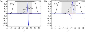
Shape of the output optimal pressure production associated with (a) axisymmetric disturbances at
 $r_{0}=48.4$
, and (b) non-axisymmetric disturbances with
 $m=40$
,
 ${\it\lambda}=7.5$
and
 $r_{0}=48.2$
. Blue line, real part of the pressure; red line, imaginary part of pressure; dashed line, rescaled base-flow temperature; solid black line, output window
 $g(r,r_{0})$
; shaded area, input window implemented by
 $\unicode[STIX]{x1D648}_{loc}$
.

properly augmented to account for reactive terms. In this expression,
 ${\rm\Delta}Q$
is the heat output of the reaction per unit mass of mixture. The premultiplying coefficient for the perturbed fuel mass fraction
 $Y_{f}^{\prime }$
identifies a variation in mixture composition with its corresponding temperature variation
 $T^{\prime }$
in the burned gases. In order to focus our study on the flame-front dynamics, the initial perturbation is taken to be localized in
 $[r_{0}-2,r_{0}+2]$
. For a given
 $r_{0}$
, we have
 $$\begin{eqnarray}\displaystyle \boldsymbol{q}^{\prime }(r)=0\quad \text{if }r<r_{0}-2\text{ or }r>r_{0}+2. & & \displaystyle\end{eqnarray}$$
The corresponding projector that accomplishes this spatial restriction is referred to as
 $\unicode[STIX]{x1D648}_{loc}$
in what follows. This windowing allows our study to focus on the whole flame structure, including the preheating area. A standard strategy would then consist in maximizing
 $\partial \Vert p^{\prime }\Vert _{comp}^{2}/\partial t$
by solving an eigenvalue problem (Schmid & Henningson Reference Schmid and Henningson2001). Instead, we propose a novel and more efficient methodology based on the maximization of the objective function
 $\mathscr{J}$
,
 $$\begin{eqnarray}\displaystyle \mathscr{J}(\boldsymbol{q}^{\prime })=\frac{1}{\sqrt{r_{eq}}}\left|\int _{0}^{\infty }\frac{\partial p^{\prime }}{\partial t}g(r,r_{0})r\,\text{d}r\right|, & & \displaystyle\end{eqnarray}$$
where
 $$\begin{eqnarray}\displaystyle r_{eq}=\frac{\left(\displaystyle \int g(r,r_{0})r\,\text{d}r\right)^{2}}{\displaystyle \int _{r_{0}-2}^{r_{0}+2}r\,\text{d}r}=\frac{\displaystyle \left(\int g(r,r_{0})r\,\text{d}r\right)^{2}}{4r_{0}}, & & \displaystyle\end{eqnarray}$$
 $\boldsymbol{q}^{\prime }$
is the perturbation state vector and
 $p^{\prime }$
is the corresponding pressure disturbance. The masking function
 $g(r,r_{0})$
ensures information extraction from the flame front and is designed to satisfy
 $g(r,r_{0})=1$
at the flame front and to smoothly decay towards zero elsewhere in the domain. The shape of
 $g(r)$
for a representative value of
 $r_{0}=48.4$
is presented by the black line in figure 3. The premultiplying factor
 $1/\sqrt{r_{eq}}$
scales the result to obtain a constant optimal value of
 $\mathscr{J}(\boldsymbol{q}^{\prime })$
for large radii by ensuring a scaling compatibility between the 2-norm-based normalization
 $\Vert \cdot \Vert _{comp}$
of the input and the form of the objective function, while maintaining consistent results at lower radii. The results stemming from (3.3) and a more classical 2-norm optimization were compared for axisymmetric configurations and found to agree within 1 % relative error. Maximization of (3.3) is preferred due to its algorithmic efficiency, as it does not require expensive large-scale eigenvalue computations. Converting our problem to a linear, discretized formulation, we have the following system of equations:
 $$\begin{eqnarray}\displaystyle \frac{\text{d}}{\text{d}t}\boldsymbol{q}^{\prime }=\unicode[STIX]{x1D63C}\,\boldsymbol{q}^{\prime },\quad p^{\prime }=\unicode[STIX]{x1D648}_{p}\boldsymbol{q}^{\prime },\quad \Vert \boldsymbol{q}^{\prime }\Vert _{comp}=\Vert \unicode[STIX]{x1D648}_{norm}\boldsymbol{q}^{\prime }\Vert _{2}, & & \displaystyle\end{eqnarray}$$
 $$\begin{eqnarray}\displaystyle & \displaystyle \boldsymbol{q}_{p}^{\prime }=\unicode[STIX]{x1D648}_{q,p}\boldsymbol{q}^{\prime }, & \displaystyle\end{eqnarray}$$
 $$\begin{eqnarray}\displaystyle & \displaystyle \int _{0}^{\infty }fg(r,r_{0})r\,\text{d}r\approx (\boldsymbol{g}_{int})^{\text{H}}\boldsymbol{f}. & \displaystyle\end{eqnarray}$$
 $\unicode[STIX]{x1D63C}$
, the matrix
 $\unicode[STIX]{x1D648}_{p}$
isolating the pressure field from the full state vector and the matrix
 $\unicode[STIX]{x1D648}_{norm}$
implementing the weights given by the norm above. Equation (3.6) extracts the pressure-related part of the perturbation
 $\boldsymbol{q}^{\prime }$
. The vector
 $\boldsymbol{q}_{p}^{\prime }$
has the same dimensionality as
 $\boldsymbol{q}^{\prime }$
and, in our case, is equal to
 $(0,0,0,p^{\prime }/({\it\gamma}-1),0)^{\text{T}}$
. The last equation recasts the integral of any quantity
 $f$
and the masking function
 $g$
in discretized form as a simple scalar product, with
 $\boldsymbol{f}$
as the discretized equivalent of
 $f$
; the complex conjugate operation is denoted by the superscript
 $^{\text{H}}$
. All the above matrices and vectors depend on the snapshot
 $\boldsymbol{q}_{0}$
and are additionally parametrized by the azimuthal wavenumber
 $m$
. Based on this notation, our optimization problem can be stated as
 $$\begin{eqnarray}\displaystyle & \displaystyle \tilde{\boldsymbol{q}}=\text{argmax}_{||\boldsymbol{q}_{1}||_{2}=1}\,\boldsymbol{g}_{int}^{\text{H}}\unicode[STIX]{x1D648}_{p}\unicode[STIX]{x1D63C}(\unicode[STIX]{x1D644}-\unicode[STIX]{x1D648}_{q,p})\unicode[STIX]{x1D648}_{norm}^{-1}\unicode[STIX]{x1D648}_{loc}\boldsymbol{q}_{1}, & \displaystyle\end{eqnarray}$$
 $$\begin{eqnarray}\displaystyle & \displaystyle \boldsymbol{q}_{opt}^{\prime }=(\unicode[STIX]{x1D644}-\unicode[STIX]{x1D648}_{q,p})\unicode[STIX]{x1D648}_{norm}^{-1}\unicode[STIX]{x1D648}_{loc}\tilde{\boldsymbol{q}}. & \displaystyle\end{eqnarray}$$
 $\boldsymbol{q}_{1}$
that, when localized in space (by
 $\unicode[STIX]{x1D648}_{loc}$
), converted to the physical space (by
 $\unicode[STIX]{x1D648}_{norm}^{-1}$
) and with its pressure component removed (by
 $\unicode[STIX]{x1D644}-\unicode[STIX]{x1D648}_{q,p}$
), maximizes its time rate of change of pressure (multiplying by
 $\unicode[STIX]{x1D648}_{p}\unicode[STIX]{x1D63C}$
) within the confines of the flame front (by multiplication with the integrating masking vector
 $\boldsymbol{g}_{int}$
). The perturbation that maximizes this expression is denoted by
 $\tilde{\boldsymbol{q}}.$
The second line retrieves the physical state corresponding to this optimal solution and removes the pressure component. The solution to the above optimization problem is straightforwardly given by
 $$\begin{eqnarray}\tilde{\boldsymbol{q}}=\frac{(\unicode[STIX]{x1D648}_{p}\unicode[STIX]{x1D63C}(\unicode[STIX]{x1D644}-\unicode[STIX]{x1D648}_{q,p})\unicode[STIX]{x1D648}_{norm}^{-1}\unicode[STIX]{x1D648}_{loc})^{\text{H}}\boldsymbol{g}_{int}}{\Vert (\unicode[STIX]{x1D648}_{p}\unicode[STIX]{x1D63C}(\unicode[STIX]{x1D644}-\unicode[STIX]{x1D648}_{q,p})\unicode[STIX]{x1D648}_{norm}^{-1}\unicode[STIX]{x1D648}_{loc})^{\text{H}}\boldsymbol{g}_{int}\Vert _{2}}.\end{eqnarray}$$
This expression shows that no large-scale and costly matrix manipulations are required so long as a multiplication with the adjoint system matrix
 $\unicode[STIX]{x1D63C}^{\text{H}}$
is provided; this makes the computation of optimal perturbations very efficient and fast. The cost functional measuring the overall acoustic output is then given for the optimal (pressure-free) perturbation by
 $$\begin{eqnarray}\mathscr{J}_{opt}\equiv \mathscr{J}(\boldsymbol{q}_{opt}^{\prime })=\frac{1}{\sqrt{r_{eq}}}\Vert (\unicode[STIX]{x1D648}_{p}\unicode[STIX]{x1D63C}(\unicode[STIX]{x1D644}-\unicode[STIX]{x1D648}_{q,p})\unicode[STIX]{x1D648}_{norm}^{-1}\unicode[STIX]{x1D648}_{loc})^{\text{H}}\boldsymbol{g}_{int}\Vert _{2}.\end{eqnarray}$$
The quantity determines the maximally achievable acoustic radiation from pressure-free initial perturbations; it is a valuable instrument in identifying regions of increased acoustic activity along the flame front. A second quantity will help us to determine the manner in which this optimal acoustic output is generated. We allow small variations
 ${\it\delta}\unicode[STIX]{x1D63C}$
of the system matrix
 $\unicode[STIX]{x1D63C}$
and record the resulting first-order variation of the cost functional,
 $$\begin{eqnarray}\displaystyle {\it\delta}\!\mathscr{J}_{opt}({\it\delta}\unicode[STIX]{x1D63C})=\frac{1}{r_{eq}\mathscr{J}_{opt}}\text{Re}\,[\tilde{\boldsymbol{q}}^{\text{H}}(\unicode[STIX]{x1D648}_{p}{\it\delta}\unicode[STIX]{x1D63C}(\unicode[STIX]{x1D644}-\unicode[STIX]{x1D648}_{q,p})\unicode[STIX]{x1D648}_{norm}^{-1}\unicode[STIX]{x1D648}_{loc})^{\text{H}}\boldsymbol{g}_{int}], & & \displaystyle\end{eqnarray}$$
thus constructing a sensitivity measure for the optimal perturbation. This measure will be used to assess the contributions of various terms in the system matrix to the optimal acoustic output.
4 Results
4.1 Axisymmetric disturbances
As a first step, we will establish a base case and assume axisymmetric perturbations, where we will find that acoustic sources are independent of vortical components and the optimal perturbation
 $\boldsymbol{q}_{opt}^{\prime }$
is dominated by a superposition of entropy and fuel mass-fraction modes. Indeed, in an axisymmetric configuration, the angular derivative
 $\partial \cdot /\partial {\it\theta}$
is null: azimuthal velocity and vorticity waves lose all influence on the rest of the flow field.
The measure
 $\mathscr{J}_{opt}$
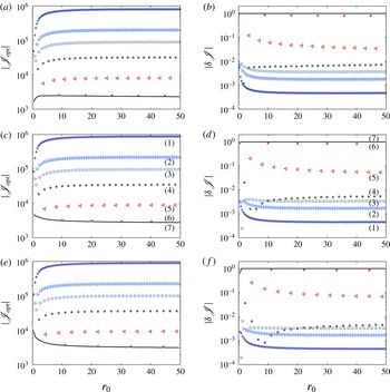
is shown, for this case, in figure 4 by the black continuous curve, demonstrating a strong preference of the flame tip (i.e. small radii of curvature) to generate acoustic waves at Lewis numbers
 $Le=1.2$
and
 $1.0$
; the opposite tendency is observed for
 $Le=0.8$
. This behaviour is compatible with pressure waves induced by heat-release rate disturbance. Chemical activity indeed intensifies with increasing mean curvature (Kidin et al.
Reference Kidin, Librovich, Roberts and Vuillermoz1984; Crighton et al.
Reference Crighton, Dowling, Ffowcs Williams, Heckl and Leppington1992; Talei et al.
Reference Talei, Brear and Hawkes2011). This finding is further corroborated by considering the sensitivity of
 $\mathscr{J}_{opt}$
to small variations in the operator
 $\unicode[STIX]{x1D63C}_{chem}$
describing the chemistry of the combustion process. We define
 $\unicode[STIX]{x1D63C}_{chem}$
as the linearized operator associated with reaction rate terms in our governing equations: it is given by a combination of (1) fuel sources due to modifications in the reaction rates and (2) energy sources due to variations of the corresponding heat-release rate. In a further step, we assume a multiplicative (scaling) change in this operator according to
 ${\it\delta}\unicode[STIX]{x1D63C}_{chem}={\it\epsilon}\unicode[STIX]{x1D63C}_{chem}$
, with
 ${\it\epsilon}\ll 1$
. The corresponding relative first-order change in
 $\mathscr{J}_{opt}$
due to this latter scaling can be defined as
 $$\begin{eqnarray}\displaystyle {\it\delta}\!\mathscr{J}=\frac{{\it\delta}\!\mathscr{J}_{opt}({\it\delta}\unicode[STIX]{x1D63C}_{chem})}{{\it\delta}\!\mathscr{J}_{chem}}. & & \displaystyle\end{eqnarray}$$
The quantity
 ${\it\delta}\!\mathscr{J}_{chem}$
denotes the expected variation of
 $\mathscr{J}_{opt}$
if
 $\mathscr{J}_{opt}$
is proportional to the chemistry operator
 $\unicode[STIX]{x1D63C}_{chem}$
. Here,
 ${\it\delta}\!\mathscr{J}_{chem}={\it\epsilon}\mathscr{J}_{opt}$
as
 ${\it\delta}\unicode[STIX]{x1D63C}_{chem}={\it\epsilon}\unicode[STIX]{x1D63C}_{chem}$
. A value of
 ${\it\delta}\!\mathscr{J}=1$
indicates that all changes in the chemistry terms convert into acoustic energy; it thus points towards acoustic output based entirely on unsteady heat release in the flame.
(a,c,e) Comparison of optimal acoustic generation for various characteristic wavelengths and axisymmetric perturbations. (b,d,f) Relative sensitivity
 ${\it\delta}\!\mathscr{J}$
of
 $\mathscr{J}_{opt}$
with respect to changes in the chemistry operator
 $\unicode[STIX]{x1D63C}_{chem}$
. A value of
 $|{\it\delta}\!\mathscr{J}|=1$
indicates that the acoustic output is solely generated by the unsteady heat-release rate. Symbols: non-axisymmetric cases with
 ${\it\lambda}=2.5{\it\lambda}_{Le}$
(1),
 ${\it\lambda}=5.0{\it\lambda}_{Le}$
(2),
 ${\it\lambda}=7.5{\it\lambda}_{Le}$
(3),
 ${\it\lambda}=12.6{\it\lambda}_{Le}$
(4),
 ${\it\lambda}=25.1{\it\lambda}_{Le}$
(5) and
 ${\it\lambda}=62.8{\it\lambda}_{Le}$
(6), with
 ${\it\lambda}_{Le}=0.89$
for
 $Le=0.8$
(a,b),
 ${\it\lambda}_{Le}=1.0$
for
 $Le=1$
(c,d) and
 ${\it\lambda}_{Le}=1.10$
for
 $Le=1.2$
(e,f). Black solid line: axisymmetric reference case (7). The parameter
 ${\it\lambda}_{Le}$
is a scaling factor that corrects for flame thickness variations with Lewis number
 $Le$
.

The results for
 ${\it\delta}\!\mathscr{J}$
are shown in figure 4. The continuous black line presents the special case of axisymmetric disturbances, which, except at the smallest radius, confirms
 ${\it\delta}\!\mathscr{J}=1$
and thus a pure generation of acoustic radiation due to reactive processes. In other words, at the flame front, in the axisymmetric case, unsteady chemistry is responsible for the coupling of entropy and fuel modes with the acoustics at all radii
 $r_{0}$
as long as
 $r_{0}>{\it\delta}_{f}$
. This finding is in agreement with experiments (Hurle et al.
Reference Hurle, Price, Sugden and Thomas1968; Candel et al.
Reference Candel, Durox, Ducruix, Birbaud, Noiray and Schuller2009). The observed variation in optimally generated noise at small radii
 $r_{0}$
can be largely accounted for by the variation of the flame velocity due to diffusive effects (Talei et al.
Reference Talei, Brear and Hawkes2011).
4.2 Non-axisymmetric disturbances
We proceed by allowing an azimuthal dependence of the flame front, thus modelling wrinkles in the flame front propagating towards the flame tip. It should be emphasized that this model neglects the influence of the tangential strain rate on the propagation of disturbances along a flame front. When approaching the flame tip, this assumption may limit the validity of our approach. In this second step, an azimuthal wavenumber
 $m$
is introduced. Owing to this new degree of freedom, the optimal perturbation
 $\boldsymbol{q}_{opt}^{\prime }$
depends not only on the flame radius but also on this azimuthal wavenumber. In order to maintain a connection between the convection of a flame wrinkle and a varying flame curvature radius (see figure 2), a meaningful choice of scale is based on considering a perturbation of constant size. For a flame of radius
 $r_{0}$
and a wrinkle described by a wavenumber
 $m$
, the characteristic wavelength of a perturbation is given by
 $$\begin{eqnarray}\displaystyle {\it\lambda}=\frac{2{\rm\pi}r_{0}}{m}. & & \displaystyle\end{eqnarray}$$
This choice enforces a balance between the azimuthal derivative operator and the radius of curvature,
 $$\begin{eqnarray}\displaystyle \frac{1}{r}\frac{\partial f}{\partial {\it\theta}}\propto \frac{m}{r_{0}}f=\frac{2{\rm\pi}}{{\it\lambda}}f. & & \displaystyle\end{eqnarray}$$
In the limit of large
 ${\it\lambda},$
azimuthal derivative terms vanish and the optimal perturbations should asymptotically approach the axisymmetric solutions. Figure 4, showing
 $\mathscr{J}_{opt}$
versus the flame radius, confirms this limit: for values of
 ${\it\lambda}$
greater than
 $50$
times the flame thickness, the optimal acoustic output coincides with the axisymmetric case (represented by the black solid line). For values of
 ${\it\lambda}<50$
, non-axisymmetric effects become important. The curves separate. In the non-axisymmetric regime, optimal perturbation
 $\boldsymbol{q}^{\prime }$
may be composed of any combination of an entropy mode, a mixture composition mode and a vortical mode. This fact provides additional degrees of freedom for the optimization, which explains why non-axisymmetric perturbations achieve higher acoustic output
 $|\mathscr{J}_{opt}|$
than axisymmetric disturbances, as shown in figure 4. Moreover, the generation of acoustic output may rely on complex mechanisms involving more than just an unsteady heat-release rate. This effect is reflected in the variation of
 $|{\it\delta}\!\mathscr{J}|$
, presented in figure 4: for
 ${\it\lambda}<50,$
the values of
 $|{\it\delta}\!\mathscr{J}|$
strongly deviate from one and converge towards zero, indicating a diminishing contribution of reactive processes (i.e. linearized chemistry) to the generation of acoustic output. This change of physics has an impact on the composition of the modes and their amplitudes at high flame curvature. We also note from inspection of figure 4 that axisymmetric disturbances for
 $Le=1$
and
 $1.2$
achieve their maximum acoustic output at low values of
 $r_{0}$
(i.e. near the flame tip for a conical flame), while non-axisymmetric perturbations produce their maximum at large radii (i.e. for planar flames). Furthermore, the shape of the pressure sources is modified as well at high
 ${\it\lambda}$
, as demonstrated in figure 3 for two representative cases. In the axisymmetric case, the pressure sources are attached to the reaction zone, whereas for large azimuthal wavenumbers the pressure sources are spread across the diffusion zone and even extend into the region of burned gases. For all cases, output pressure sources were found to have a uniform phase along the radial direction
 $r$
: this is a consequence of the integral form of our objective function
 $\mathscr{J}$
. These phenomena hold for all Lewis-number values considered in this study. The most significant difference observed is related to the asymptotic behaviour of axisymmetric disturbances at low radii. For
 $Le=1.2$
and
 $1.0$
, pressure-source amplitudes increase with curvature, while they decrease for the case of
 $Le=0.8$
.
Last, it should be noted that the choice of the scaling factor
 $r_{eq}$
may change the value of
 $|\mathscr{J}_{opt}|$
at low radii. However, the relative behaviour of these curves will be unchanged, as this scaling factor is identical for all cost functionals. Besides, it was checked that other choices of
 $r_{eq}$
do not change the sign of the slope of the curves at small
 $r_{0}$
as long as
 $r_{eq}\sim r_{0}$
.
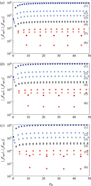
Comparison of acoustic output for modes optimizing
 $\mathscr{J}$
(circles) and modes with maximal vorticity changes optimizing
 $\mathscr{J}_{2}$
(squares) for
 ${\it\lambda}=2.5$
(1),
 ${\it\lambda}=5.0$
(2),
 ${\it\lambda}=7.5$
(3),
 ${\it\lambda}=12.6$
(4),
 ${\it\lambda}=25.1$
(5) and
 ${\it\lambda}=62.8$
(6) and for Lewis number
 $Le=0.8$
(a), 1.0 (b) and 1.2 (c).

Understanding the transition of pressure generation at the flame front from large to small wavelengths is of importance and warrants further analysis. To this end, we propose a vortex–sound mechanism (see e.g. Powell Reference Powell1964) as the dominant process for the generation of pressure output at low wavelength and investigate the validity of this assumption. Hence, a new objective function is introduced according to
 $$\begin{eqnarray}\displaystyle \mathscr{J}_{2}(q^{\prime })=\frac{1}{\sqrt{r_{eq}}}\left|\int _{0}^{\infty }\frac{\partial {\it\zeta}^{\prime }}{\partial t}g(r,r_{0})r\,\text{d}r\right|, & & \displaystyle\end{eqnarray}$$
where
 ${\it\zeta}^{\prime }$
denotes the vorticity of the linear perturbation. The maximization of this cost functional leads again to an optimal pressure-free perturbation
 $\boldsymbol{q}_{opt,2}^{\prime }$
. The acoustic output computed by optimizing either the previous cost functional (emphasizing pressure generation processes)
 $\mathscr{J}_{opt}=\mathscr{J}(\boldsymbol{q}_{opt}^{\prime })$
or the above cost functional (emphasizing vorticity-based process)
 $\mathscr{J}_{opt,2}=\mathscr{J}(\boldsymbol{q}_{opt,2}^{\prime })$
is compared in figure 5. In this figure, the circles are identical to the markers shown in figure 4(a,c,e). At low values of
 ${\it\lambda}$
, we observe a close agreement between the two optimization problems, indicating a dominant contribution of vorticity to the generation of sound. This may also have implications on the modal behaviour at low values of
 $r_{0}$
: when the mean flame curvature is important, vortices interact strongly and dominate the acoustic activity. At higher values of
 ${\it\lambda}$
, at least one order of magnitude separates the values of
 $\mathscr{J}$
computed by the two methods, and the pressure field generated by vorticity variations becomes negligible.
As a conclusion, for large-scale perturbations, the unsteady heat-release rate constitutes the dominant source of sound, while for disturbance wavelengths of the order of the planar flame thickness, vorticity dynamics becomes the prevailing mechanism in acoustic wave generation.
5 Discussion and conclusions
In this paper the influence of mean flame curvature
 $r_{0}$
and small-amplitude flame wrinkles (characterized by a wavelength
 ${\it\lambda}$
) on the production of acoustic output has been addressed by posing an optimization problem for a generic configuration. More specifically, the flame dynamics has been studied by considering an axisymmetric, laminar, imploding flame front upon which azimuthal disturbances have been superimposed, and their dynamics along the flame front has been investigated. The choice of optimization variable (in our case, unsteady heat-release rate or vorticity) has allowed us to quantify the contribution of various noise-generation mechanisms to the overall acoustic output.
The main characteristic length of the problem is the flame thickness
 ${\it\delta}_{f}$
, and the wavelength
 ${\it\lambda}$
, quantifying flame wrinkles, has been non-dimensionalized using
 ${\it\delta}_{f}$
(as have all other spatial scales). From our analysis, two distinct behaviours can be observed. For large-scale perturbations (with
 ${\it\lambda}>50$
), the unsteady heat-release rate is the dominant contributor to acoustic radiation. As a consequence, the maximum of our objective functional
 $\mathscr{J}_{opt}$
increased with the flame-front curvature for
 $r_{0}<10$
. In contrast, for small perturbations (with
 ${\it\lambda}<8$
), changes in vorticity become the prevalent sources of pressure fluctuations and thus acoustics. The values of
 $\mathscr{J}_{opt}$
then decrease for high mean curvature (
 $r_{0}<10$
). This transition between two contrasting behaviours has important physical implications.
The importance of vorticity in the generation of noise is well known for non-reactive flows (Powell Reference Powell1964); in combustion systems, on the other hand, the contribution of vorticity to acoustics is far less established. Indeed, experimentally, a flame submitted to a large-scale vortex (
 ${\it\lambda}\gg 1$
) will simply roll up (Renard et al.
Reference Renard, Thévenin, Rolon and Candel2000). At smaller scales, however, Poinsot, Veynante & Candel (Reference Poinsot, Veynante and Candel1991) and Roberts & Driscoll (Reference Roberts and Driscoll1991) showed that vortices (of constant vortex strength) were unable to disrupt the flame front. The transition between these two behavioural regimes was observed for
 $3<{\it\lambda}<100$
. The transitional values of
 ${\it\lambda}$
found in our study are compatible with these simulations and experiments. Our results also suggest two distinct scenarios. At large scales, flame–vortex interaction may lead to an increased flame surface variation and consequently to the generation of sound via an unsteady heat-release rate. At small scales, the vortex is unable to disrupt the flame front, is partly absorbed by the flame structure and generates high local pressure levels. This result was observed to hold across all Lewis numbers considered here.
If confirmed by further experiments or simulations, this physical phenomenon will strongly influence the root-mean-square values of the near-field pressure. Moreover, our analysis shows that the flame diffusion thickness
 ${\it\delta}_{f}$
plays an essential role as the crucial characteristic length. The effects of complex chemistry also need to be assessed. Energy exchanges between entropy, vorticity, mixture fraction and acoustic modes at the flame surface is a complex and sensitive topic, further complicated by nonlinear effects rising quickly in flames. A proper validation of these results by nonlinear simulations or experiments would greatly enhance our understanding of combustion noise and flame dynamics and contribute to a mechanistic and physical picture of sound generation in reactive flows.
Acknowledgement
We would like to thank G. Lerisson for providing the initial impulse behind this project.