1 Introduction
The dynamics and rheology of complex mixtures of immiscible fluids are important areas of study due to the significance of multiphase flows in numerous industrial processes. Moreover, deformable ellipsoids are common abstractions used to model the dispersed phase microstructure in flowing soft matter systems including emulsions (Vermant et al. Reference Vermant, Van Puyvelde, Moldenaers, Mewis and Fuller1998) and polymers and polymer blends (Lee & Park Reference Lee and Park1994). Rallison (Reference Rallison1980) and Stone (Reference Stone1994) have extensively discussed and reviewed the subject of drop deformation from theoretical and experimental perspectives. Furthermore, numerous models, at different levels of complexity, have been proposed to capture various aspects of droplet behaviour in viscous flows.
The most important advances in modelling the rheology of suspensions have been realized by connecting the microscopic analysis of the detailed flow field around the suspended particles to the macroscopic rheology of the suspension (Einstein Reference Einstein1906, Reference Einstein1911). This pioneering work by Einstein in the dilute limit of solid particle suspensions has been extended to describe higher-order concentration effects and/or droplet particles with finite internal viscosity (Taylor Reference Taylor1932, Reference Taylor1934; Batchelor Reference Batchelor1970; Happel & Brenner Reference Happel and Brenner1983). However, even for dilute suspensions, there are higher-order effects that give rise to normal stress contributions (Schowalter, Chaffey & Brenner Reference Schowalter, Chaffey and Brenner1968; Frankel & Acrivos Reference Frankel and Acrivos1970; Raja, Subramanian & Koch Reference Raja, Subramanian and Koch2010), which therefore cannot be described by a modified viscosity corresponding to a generalized Newtonian model. Moreover, for suspensions of deformable liquid particles, i.e. emulsions, the macroscopic flow induces anisotropy in the shape of the emulsion droplet as well as in the neighbour distribution. Therefore, in addition to the rheology, one has to also describe the flow-induced anisotropic microstructure. This work shows how one can take advantage of the shape anisotropy that emerges naturally as a characteristic of the system at the microscopic level to describe the overall rheological behaviour at the macroscopic level in dilute emulsion suspensions. To connect the microscopic and macroscopic levels in emulsions with ellipsoidal morphology, an internal second-order conformation tensor that describes the deformed ellipsoidal shape of individual droplets is used in this work. Following guidelines from non-equilibrium thermodynamics, we develop an evolution equation for the ellipsoidal droplet as well as an expression for the extra stress tensor which emulates those arising from independent asymptotic results from microscopic theory (Schowalter et al. Reference Schowalter, Chaffey and Brenner1968; Frankel & Acrivos Reference Frankel and Acrivos1970) in the limit of dilute emulsions.
Some of the earliest studies on the micromechanics of single droplets in viscometric flows were carried out by Taylor (Reference Taylor1932, Reference Taylor1934), Oldroyd (Reference Oldroyd1953) and Batchelor (Reference Batchelor1970). Soon thereafter, these ideas were extended to multiple droplets in viscous flows by Choi & Schowalter (Reference Choi and Schowalter1972), Palierne (Reference Palierne1990) and Delaby, Muller & Ernst (Reference Delaby, Muller and Ernst1995). However, since these analytical calculations, as well as corresponding numerical simulations (Rallison & Acrivos Reference Rallison and Acrivos1978; Rallison Reference Rallison1984; Loewenberg & Hinch Reference Loewenberg and Hinch1996), are often too involved to be used directly in engineering applications, the need for more coarse-grained modelling approaches is apparent. At the coarse-grained level of modelling, either covariant or contravariant tensors are used as internal variables to describe the internal microstructure, depending on the morphology of interest (Minale Reference Minale2010). Mathematically, these two descriptions are related through an inverse, as the inverse of the covariant tensor is a contravariant tensor, and vice versa (Edwards & Dressler Reference Edwards and Dressler2003). Nevertheless, such a one-to-one relationship should not be considered to mean that there is necessarily a one-to-one correspondence between the tensor descriptions. The validity of the inverse relationship also depends on the physical interpretations and definitions of the tensors at hand. To date, the modelling of interfaces in emulsions has been carried out primarily either through interface or area tensors (which are covariant tensor objects) or alternatively through ellipsoid morphology tensors (which can be cast as either covariant or contravariant tensor objects).
The interfacial tensor (Doi & Ohta Reference Doi and Ohta1991; Wetzel & Tucker Reference Wetzel and Tucker1999; Almusallam, Larson & Solomon Reference Almusallam, Larson and Solomon2000) is a second-order tensor object which is related to the second moment of the interface density function, whose primary variable is the unit vector normal to the interface. Physically, the interfacial tensor represents the average size and orientation of the interface. In this approach, the surface area of the interface is proportional to the first invariant of the area tensor and can be computed exactly. On the other hand, the volume of the dispersed phase enclosed by the interface is difficult to calculate, and approximate relationships and/or closure rules must be used (Doi & Ohta Reference Doi and Ohta1991; Wetzel & Tucker Reference Wetzel and Tucker1999; Almusallam et al. Reference Almusallam, Larson and Solomon2000; Almusallam, Larson & Solomon Reference Almusallam, Larson and Solomon2004). As a consequence, volume conservation is difficult to enforce in modelling incompressible fluids enclosed by an interface. Such models have been widely studied (Takahashi et al. Reference Takahashi, Kurashima, Noda and Doi1994; Guenther & Baird Reference Guenther and Baird1996; Vinckier, Moldenaers & Mewis Reference Vinckier, Moldenaers and Mewis1996), as constitutive equations can be developed based on the stress tensor of Batchelor (Reference Batchelor1970) which admits an interface tensor. A review of this class of models is presented by Almusallam et al. (Reference Almusallam, Larson and Solomon2004) and Minale (Reference Minale2010). However, because of the above-mentioned difficulties in implementing the volume conservation constraint, we choose not to use this internal tensor variable any further within the present work.
Instead, of primary interest for this work are conformation tensor models that use the geometrical deformation of an initially spherical droplet to describe emulsion morphology. These ellipsoid morphology tensors can be categorized as either contravariant (Maffettone & Minale Reference Maffettone and Minale1998) or covariant (Wetzel & Tucker Reference Wetzel and Tucker2001), with these two forms being both mathematically and physically equivalent. Moreover, it should be noted that ellipsoid morphology tensors can be related to the interfacial tensor, but the relationship is not one to one (Wetzel & Tucker Reference Wetzel and Tucker1999). In both contravariant and covariant cases, the eigenvectors of the ellipsoidal tensor are along the direction of the principal axes of the ellipsoid. However, in the contravariant tensor, the eigenvalues are proportional to the square of the semi-axes of the ellipsoid, while in the covariant tensor, they are inversely proportional. Therefore, the covariant tensor is formally the inverse of the contravariant one. In either tensor description, a connection can be made between the canonical form of an ellipsoid equation,
 $x^{2}L^{2}+y^{2}/B^{2}+z^{2}/W^{2}=1$
(where
 $L$
,
 $B$
and
 $W$
are the ellipsoid semi-axes and
 $x$
,
 $y$
and
 $z$
coordinates on the ellipsoid surface) and the quadratic forms
 $\unicode[STIX]{x1D63E}\boldsymbol{ : }\boldsymbol{q}\,\boldsymbol{q}=1$
and
 $\unicode[STIX]{x1D63E}^{-1}\boldsymbol{ : }\boldsymbol{q}\,\boldsymbol{q}=1$
(where the vector
 $\boldsymbol{q}=[x\;y\;z]^{\text{T}}$
) for the covariant and contravariant forms respectively. As a result, the volume of an emulsion droplet is related to the third invariant (i.e. the determinant) of the conformation tensor, and volume conservation can be strictly enforced by requiring that the third invariant is constant. In contrast, in this formulation, it is the surface area that is difficult to calculate, necessitating the use of approximate relationships, as analytical expressions only exist for specialized ellipses. Covariant (Jackson & Tucker Reference Jackson and Tucker2003; Yu & Bousima Reference Yu and Bousima2003; Yu & Zhou Reference Yu and Zhou2007) and contravariant (Minale Reference Minale2004) ellipsoid morphology tensor models have found particular success in describing experimentally observed droplet morphology in the vicinity of overcritical capillary numbers.
The models mentioned so far are highly phenomenological. Significant advances can be made by employing a non-equilibrium thermodynamics (NET) framework which combines in a systematic and consistent fashion Hamiltonian mechanics and dissipation (Grmela Reference Grmela, Casas-Vazquez and Jou1991, Reference Grmela1993). In this framework, the reversible dynamics is developed based on a Poisson bracket description of Hamiltonian mechanics. The challenge lies in prescribing the irreversible dynamics that gives rise to the dissipation. Beris & Edwards (Reference Beris and Edwards1994) systematically described the single-generator approach, in which the irreversible dynamics is also generated from the system Hamiltonian through a dissipation bracket, and demonstrated its applicability towards describing classical viscoelasticity. Moving beyond this, The general equation for reversible and irreversible coupling (GENERIC), developed by Grmela & Öttinger (Reference Grmela and Öttinger1997) and Öttinger & Grmela (Reference Öttinger and Grmela1997), allows for the generation of reversible and irreversible dynamics based on the Hamiltonian and entropy functionals respectively. A detailed comparison of these developments which shows their equivalence as far as macroscopic modelling is concerned is provided by Edwards (Reference Edwards1998) and Edwards, Beris & Öttinger (Reference Edwards, Beris and Öttinger1998). Several authors (Grmela & Ait-Kadi Reference Grmela and Ait-Kadi1998; Grmela, Ait-Kadi & Utracki Reference Grmela, Ait-Kadi and Utracki1998; Wagner, Öttinger & Edwards Reference Wagner, Öttinger and Edwards1999; Wagner et al. Reference Wagner, Öttinger and Edwards1999) have analysed the Doi–Ohta model from a thermodynamics perspective using the GENERIC formalism. They concluded that the dynamical equations proposed in the Doi–Ohta model are thermodynamically consistent. Although attempts have been made to develop interfacial tensor models for ellipsoidal droplet morphologies (Almusallam et al. Reference Almusallam, Larson and Solomon2000, Reference Almusallam, Larson and Solomon2004; Edwards & Dressler Reference Edwards and Dressler2003), the volume constraint is much more difficult to implement under these conditions than in the ellipsoid morphology tensor approach. This further motivates our efforts in the present work to develop a thermodynamically consistent ellipsoidal morphology tensormodel.
Some previous work has already been devoted towards understanding the thermodynamic validity of ellipsoid morphology tensor model equations. Ait-Kadi et al. (Reference Ait-Kadi, Ramazani, Grmela and Zhou1999) outlined the GENERIC development of a contravariant tensor model subject to a constant determinant constraint. However, this model was presented in an abstract fashion, with the conformation tensor not identified with any specific microstructure, the free energy density provided as a general function of the conformation tensor invariants, and with no affine deformation. Thus, it has no direct applicability as a contravariant emulsion morphology model. Building further upon this work, Grmela, Bousmina & Palierne (Reference Grmela, Bousmina and Palierne2001) introduced a non-affine contribution to the convected time derivative and, among other things, showed how formally a conformation-based evolution equation that resembles that of the Maffettone & Minale (Reference Maffettone and Minale1998) model can be realized within the GENERIC framework for a specific form of the free energy expression. However, the conformation tensor they chose was different from that appearing in the Maffettone & Minale (Reference Maffettone and Minale1998) model, in that although it also corresponded to a symmetric second-order tensor whose eigenvectors were the axes of the ellipsoidal droplet, they chose the lengths of the semi-axes of the ellipsoid as its eigenvalues (as emerges from the expression offered for the total volume
 $V_{B}$
of the dispersed fluid
 $(B)$
as
 $nV\det (\unicode[STIX]{x1D657})$
, where
 $n$
is the droplet number density,
 $V$
is the total volume and
 $\unicode[STIX]{x1D657}$
is the conformation tensor that they used). Consequently,
 $\unicode[STIX]{x1D657}$
is the square root of the conformation tensor
 $\unicode[STIX]{x1D63E}$
that appears in Maffettone & Minale (Reference Maffettone and Minale1998), and if the latter (as we will show below) is indeed a contravariant tensor, the first one is not, and in consequence it is not suitable to use as a primitive tensor variable as its reversible part does not transform as either a contravariant or covariant tensor (the only two objective tensors for which a Poisson bracket is available). In addition, the free energy expression that Grmela et al. (Reference Grmela, Bousmina and Palierne2001) used was arbitrary and not consistent with the expected form of the surface-free energy when expressed in terms of the conformation tensor, necessitating further improvements.
Subsequently, Grmela et al. (Reference Grmela, Ammar, Chinesta and Maîtrejean2014), advanced a free energy expression specifically to express the surface energy of the droplets. In this free energy expression, the surface area was identified with the second invariant of the conformation tensor, which is a reasonable but significant approximation. Despite this improvement, the main problem with the latest Grmela et al. (Reference Grmela, Ammar, Chinesta and Maîtrejean2014) model is that the conformation tensor used is, like
 $\unicode[STIX]{x1D657}$
before, identified with the square root of the Maffettone & Minale (Reference Maffettone and Minale1998) contravariant conformation tensor, and therefore this is not a contravariant tensor. A further corroborative proof that this is the meaning of the second-order tensor used by Grmela et al. (Reference Grmela, Ammar, Chinesta and Maîtrejean2014) is that it has units of length, leading to a second invariant with units of length squared, therefore making the second invariant suitable to represent the ellipsoid surface as they did. As a consequence, if the correct physics of the Maffettone & Minale (Reference Maffettone and Minale1998) physical picture is to be followed, it is the square of the tensor used by Grmela et al. (Reference Grmela, Ammar, Chinesta and Maîtrejean2014) that is contravariant and for which a relevant Poisson bracket can be built to represent its reversible dynamics; treating its square root as the contravariant tensor object following Grmela et al. (Reference Grmela, Ammar, Chinesta and Maîtrejean2014) makes the developed model equations inconsistent with the physics of emulsion deformation. Still, the model equations developed in Grmela et al. (Reference Grmela, Ammar, Chinesta and Maîtrejean2014) can be used, but need to be considered as phenomenological approximations of the underlying physics of droplet deformation dynamics.
Therefore, the need for a physically based and thermodynamically consistent emulsion-morphology-based contravariant tensor model still remains. Thermodynamic consistency is important because through it one avoids unnatural model instabilities and/or aphysical results corresponding to a negative rate of entropy production (Beris & Edwards Reference Beris and Edwards1994). It also guarantees physical results for general flows, not just simple shear flow. In addition, it highlights the intimate connection between the conformation tensor and the stress tensor, which underlies the rheological response that is absent in phenomenological models like the MM model (Maffettone & Minale Reference Maffettone and Minale1998). In these models, the only way to obtain the deformed droplet-induced stress is by using the stress expression of Batchelor (Reference Batchelor1970). However, this limits the use of these models to equal disperse and continuous phase viscosities, because if they are different the interfacial velocity (which is not accessible through a phenomenological model) is needed. To move beyond current model capabilities, a thermodynamically consistent ellipsoidal emulsion (TCEE) model is systematically developed in the present work and validated by showing its consistency against known independent microscopic asymptotic theories in the limit of small capillary numbers. In parallel, the results from asymptotic theory are used to a priori determine all parameters of the TCEE model, thus allowing for the realization of a purely predictive macroscopic model.
The key essence of this work is to demonstrate that it is possible to construct a macroscopic theory for dilute emulsion flow which is consistent with known microscopic results for both the microstructure and the stress tensor. In this way, the number of adjustable parameters is significantly reduced. Furthermore, moving beyond traditional phenomenological models (such as Maffettone & Minale (Reference Maffettone and Minale1998) and Wetzel & Tucker (Reference Wetzel and Tucker2001)), which place an emphasis on only describing droplet deformation and orientation, the present work introduces a systematic approach towards developing corresponding expressions for the stresses consistent with both the droplet microstructure and available theoretical microscopic results. In this way, this work distinguishes itself even from related thermodynamically consistent emulsion flow models in the literature (Grmela et al.
Reference Grmela, Ammar, Chinesta and Maîtrejean2014). It needs to be said that although the present work is restricted to the (usual in material constitutive equations) particle inertialess limit, the thermodynamic approach followed can also be generalized to include particle inertia effects (characterized by the particle Reynolds number), as addressed in a subsequent publication (Mwasame, Wagner & Beris Reference Mwasame, Wagner and Beris2017). Furthermore, we need to stress that in order to keep the complexity to a minimum, we opted here to offer a version of the theory with the minimum complexity necessary to match available microscopic theory to
 $O(1)$
in the conformation tensor evaluation and
 $O(Ca^{2})$
in the stress. However, if so needed, the approach we present can be extended, at the expense of additional complexity, to also accommodate additional information from asymptotic theory and/or experimental results, while still preserving the consistency with the asymptotic expression employed in this work.
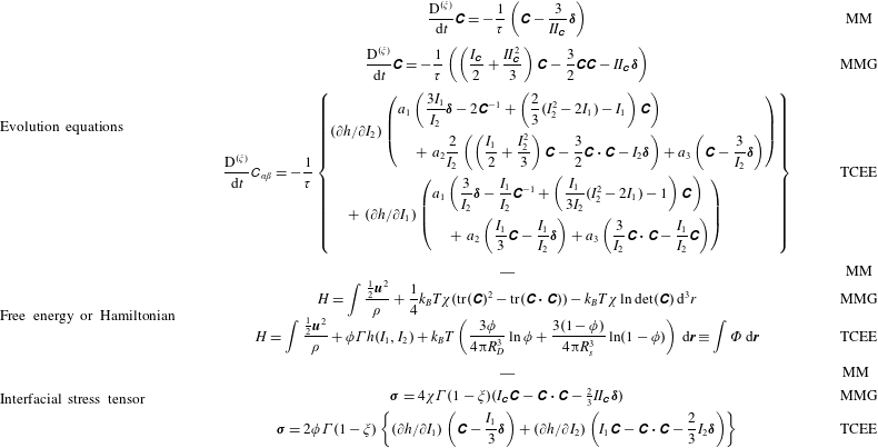
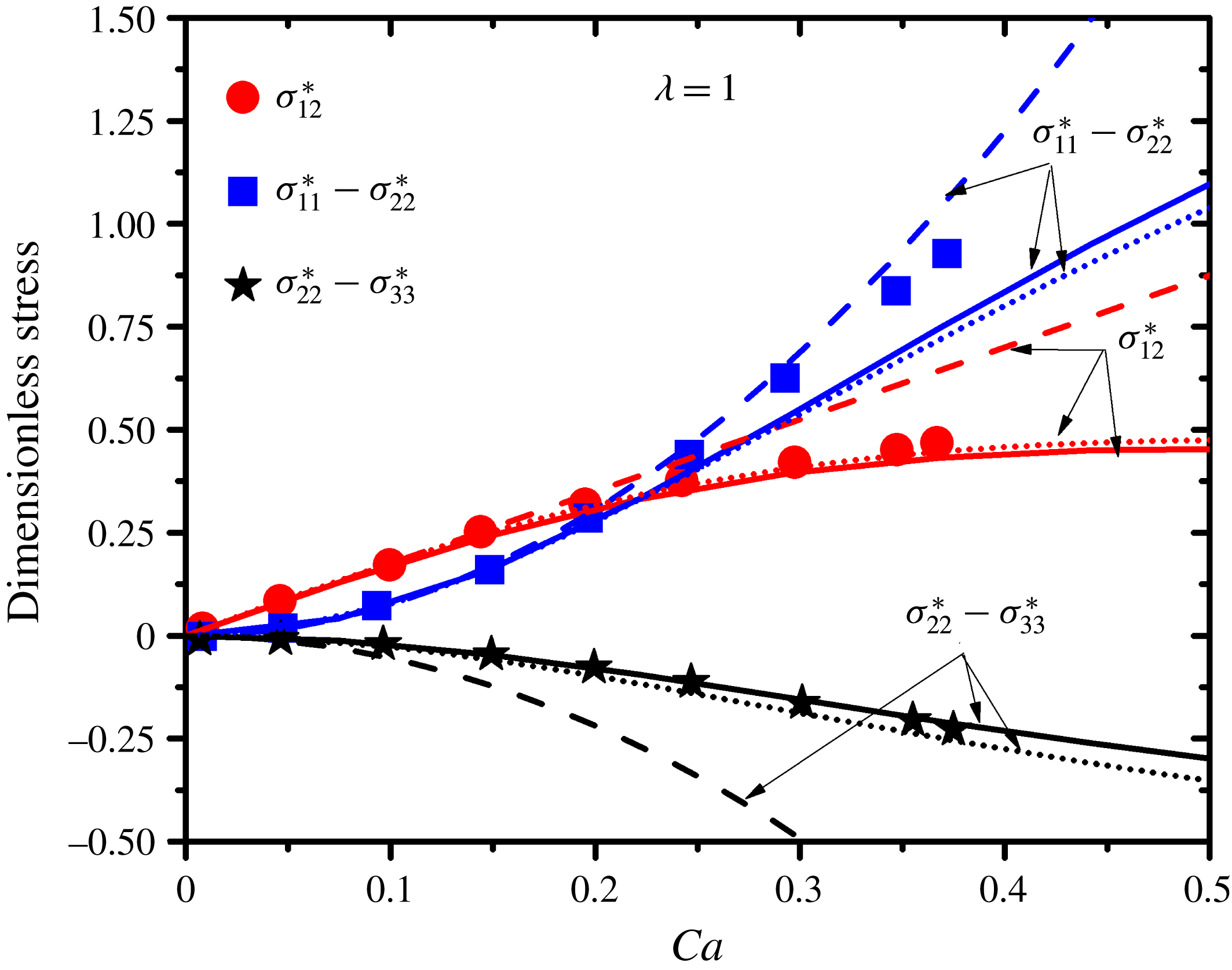
In the next section, we summarize two contravariant ellipsoid morphology models from the literature, the MM and MMG models, as well as asymptotic results from microscopic theory. In § 3, we first present the complete description of the Poisson and dissipative bracket structure in the presence of a unit determinant constraint, following closely the work of Edwards et al. (Reference Edwards, Dressler, Grmela and Ait-Kadi2003), as well as a description of the correct subspaces in which the Volterra derivative must be evaluated. Then, we describe the form of the surface-free energy assuming an ellipsoidal droplet. Moreover, we show how the model parameters can be selected so that the TCEE model is fully compatible with existing asymptotic expansions previously developed by Schowalter et al. (Reference Schowalter, Chaffey and Brenner1968) and also Frankel & Acrivos (Reference Frankel and Acrivos1970). In § 4, the TCEE model predictions are compared with the MM model as well as with experimental data by Torza, Cox & Mason (Reference Torza, Cox and Mason1972). In that section, we also demonstrate the consistency of the TCEE model with theoretical results by Taylor (Reference Taylor1934) and Chaffey & Brenner (Reference Chaffey and Brenner1967) at small capillary numbers. Finally, in § 5, we present our conclusions.
2 Previous ellipsoid morphology models and asymptotic results in the literature
This section provides a brief overview of two conformation-tensor-based models designed for emulsions that comprise Newtonian constituents as well as some relevant asymptotic results from microscopic investigations.
2.1 The Maffettone and Minale (MM) model
Maffettone & Minale (Reference Maffettone and Minale1998) developed a specialized and phenomenological expression, subsequently referred to as the MM model, to describe the dynamics of non-coalescing and non-breaking ellipsoidal droplets in a general flow field. The droplet morphology is described by a contravariant second-rank structural tensor
 $\unicode[STIX]{x1D63E}$
subject to a unit determinant constraint to guarantee that the volume of the drop is conserved. This model is applicable to dilute and semi-dilute polymer blends, with ellipsoidal morphology, in which the droplet relaxation is expected to be minimally affected by hydrodynamic interactions between droplets. The validity of such an assumption is supported by literature results (Vinckier et al.
Reference Vinckier, Moldenaers and Mewis1996; Vinckier, Mewis & Moldenaers Reference Vinckier, Mewis and Moldenaers1997) which show that it is possible to predict the rheological response of a polymer blend when the deformation of a single droplet is known as a function of the shear rate. However, unlike the Doi–Ohta model, the evolution equation for
 $\unicode[STIX]{x1D63E}$
has no accompanying stress equation.
In the MM model, the eigenvectors and eigenvalues of
 $\unicode[STIX]{x1D63E}$
correspond to the direction and square of the magnitude respectively of the dimensionless principal semi-axes of the ellipsoidal droplet, the lengths of the semi-axes having been made dimensionless using the equilibrium droplet radius. As a result of the non-dimensionalization, we can express the volume constraint resulting from the mass preservation of a droplet (assumed to be incompressible and no breakage or coalescence takes place) by taking the determinant of
 $\unicode[STIX]{x1D63E}$
(which is proportional to the square of the volume of the ellipsoidal droplet that it represents given its definition above) constant and equal to unity,
 $I_{3}\equiv \det (\unicode[STIX]{x1D63E})=1$
. The relaxation mechanism for the droplet dynamics is then provided by the surface tension which acts to return the deformed ellipsoid to a spherical shape.
The dynamical equation for the conformation tensor variable provided by Maffettone & Minale (Reference Maffettone and Minale1998) is
 $$\begin{eqnarray}\frac{\text{D}\unicode[STIX]{x1D63E}}{\text{d}t}-(\unicode[STIX]{x1D734}\boldsymbol{\cdot }\unicode[STIX]{x1D63E}-\unicode[STIX]{x1D63E}\boldsymbol{\cdot }\unicode[STIX]{x1D734})+(\unicode[STIX]{x1D709}-1)(\unicode[STIX]{x1D63F}\boldsymbol{\cdot }\unicode[STIX]{x1D63E}+\unicode[STIX]{x1D63E}\boldsymbol{\cdot }\unicode[STIX]{x1D63F})=-\frac{1}{\unicode[STIX]{x1D70F}}\left(\unicode[STIX]{x1D63E}-\frac{3}{I_{2}}\unicode[STIX]{x1D739}\right).\end{eqnarray}$$
The left-hand side of (2.1) is the Gordon–Schowalter time derivative defined in terms of the rate of strain
 $(\unicode[STIX]{x1D63F})$
and vorticity tensors
 $(\unicode[STIX]{x1D734})$
and the dimensionless non-affine parameter
 $\unicode[STIX]{x1D709}$
. The rate of strain tensor,
 $\unicode[STIX]{x1D63F}$
, is defined as
 $$\begin{eqnarray}\unicode[STIX]{x1D63F}={\textstyle \frac{1}{2}}((\unicode[STIX]{x1D735}\,\boldsymbol{V})^{\text{T}}+(\unicode[STIX]{x1D735}\,\boldsymbol{V})),\end{eqnarray}$$
while the vorticity tensor,
 $\unicode[STIX]{x1D734}$
, is defined as
 $$\begin{eqnarray}\unicode[STIX]{x1D734}={\textstyle \frac{1}{2}}((\unicode[STIX]{x1D735}\,\boldsymbol{V})^{\text{T}}-(\unicode[STIX]{x1D735}\,\boldsymbol{V})).\end{eqnarray}$$
In addition,
 $I_{2}$
describes the second invariant of the conformation tensor
 $\unicode[STIX]{x1D63E}$
, defined as
 $$\begin{eqnarray}I_{2}={\textstyle \frac{1}{2}}(\text{tr}(\unicode[STIX]{x1D63E})^{2}-\text{tr}(\unicode[STIX]{x1D63E}\boldsymbol{\cdot }\unicode[STIX]{x1D63E})),\end{eqnarray}$$
where
 $\text{tr}(\text{})$
is the trace and
 $\text{tr}(\unicode[STIX]{x1D63E})$
represents the first invariant,
 $I_{1}$
, of
 $\unicode[STIX]{x1D63E}$
. Finally, in (2.1),
 $\unicode[STIX]{x1D70F}$
represents a characteristic relaxation time. It should be noted that the constraint
 $I_{3}=\det (\unicode[STIX]{x1D63E})=1$
, once satisfied by the initial conditions, is duly preserved by the dynamics described by (2.1).
The parameters
 $\unicode[STIX]{x1D709}$
and
 $\unicode[STIX]{x1D70F}$
in (2.1) can now be expressed in terms of the original symbols employed by Maffettone & Minale (Reference Maffettone and Minale1998). The relaxation time
 $\unicode[STIX]{x1D70F}$
entering (2.1) is defined in terms of the original parameters as
 $\unicode[STIX]{x1D70F}\equiv \unicode[STIX]{x1D70F}_{C}/f_{1}$
, where
 $\unicode[STIX]{x1D70F}_{C}$
is a characteristic time defined as
 $\unicode[STIX]{x1D70F}_{C}\equiv \unicode[STIX]{x1D707}a/\unicode[STIX]{x1D6FE}$
, with
 $\unicode[STIX]{x1D6FE}$
the surface tension,
 $\unicode[STIX]{x1D707}$
the continuous phase viscosity and
 $a$
the equilibrium radius of the emulsion droplet, while
 $f_{1}=40(\unicode[STIX]{x1D706}+1)/((19\unicode[STIX]{x1D706}+16)(2\unicode[STIX]{x1D706}+3))$
is assumed to be a function of the viscosity ratio,
 $\unicode[STIX]{x1D706}$
, where
 $\unicode[STIX]{x1D706}\equiv \unicode[STIX]{x1D707}_{d}/\unicode[STIX]{x1D707}$
and
 $\unicode[STIX]{x1D707}_{d}$
is the dispersed phase viscosity. Finally,
 $\unicode[STIX]{x1D709}=1-f_{2}$
, where
 $f_{2}=5/(2\unicode[STIX]{x1D706}+3)$
, and takes values ranging from 0 to
 $5/3$
.
A key observation from the MM model is that the time derivative used for the
 $\unicode[STIX]{x1D63E}$
tensor, as expressed by the left-hand side of (2.1), is the Gordon–Schowalter time derivative (Gordon & Schowalter Reference Gordon and Schowalter1972). A value of
 $\unicode[STIX]{x1D709}=1$
is the limit of full non-affine motion, and the left-hand side of (2.1) reduces to the Jaumann derivative (Jaumann Reference Jaumann1911). On the other hand, a value
 $\unicode[STIX]{x1D709}=0$
corresponds to fully affine motion, and the left-hand side of (2.1) reduces to the upper-convected time derivative. Moving forward, the Gordon–Schowalter time derivative will be denoted by the following shorthand:
 $$\begin{eqnarray}\frac{\text{D}^{(\unicode[STIX]{x1D709})}\unicode[STIX]{x1D63E}}{\text{d}t}\equiv \frac{\text{D}\unicode[STIX]{x1D63E}}{\text{d}t}-(\unicode[STIX]{x1D734}\boldsymbol{\cdot }\unicode[STIX]{x1D63E}-\unicode[STIX]{x1D63E}\boldsymbol{\cdot }\unicode[STIX]{x1D734})+(\unicode[STIX]{x1D709}-1)(\unicode[STIX]{x1D63F}\boldsymbol{\cdot }\unicode[STIX]{x1D63E}+\unicode[STIX]{x1D63E}\boldsymbol{\cdot }\unicode[STIX]{x1D63F}).\end{eqnarray}$$
The next observation is that the relaxation term in the MM model incorporates a nonlinear dependence on the second invariant. We note that (2.1) may be considered to be phenomenological and does not by itself allow one to obtain an expression for a rigorous stress tensor except in the very specific limit of
 $\unicode[STIX]{x1D706}=1$
, where Batchelor’s stress formula can be used (Batchelor Reference Batchelor1970). This is the one of the motivations for the development of a recent model derived by Grmela et al. (Reference Grmela, Ammar, Chinesta and Maîtrejean2014), which is described next.
2.2 The MMG model
Applying a thermodynamically consistent methodology to a contravariant internal conformation tensor, Grmela et al. (Reference Grmela, Ammar, Chinesta and Maîtrejean2014) derived a macroscopic phenomenological approximation of the MM model, referred to here as the MMG model. This model is applicable to isothermal emulsions and also includes an extension towards describing emulsions with non-ellipsoidal shapes. The main advantage of the Grmela et al. (Reference Grmela, Ammar, Chinesta and Maîtrejean2014) approach is that starting from an expression for the free energy,
 $H$
, a constitutive equation for the stress tensor is also derived consistently from the NET formalism. Their free energy expression, in terms of a dimensional conformation tensor, was specified by
 $$\begin{eqnarray}H=\int \left(\frac{\frac{1}{2}\boldsymbol{u}^{2}}{\unicode[STIX]{x1D70C}}+\overline{\unicode[STIX]{x1D6E4}}\unicode[STIX]{x1D712}(\text{tr}(\overline{\unicode[STIX]{x1D63E}})^{2}-\text{tr}(\overline{\unicode[STIX]{x1D63E}}\overline{\unicode[STIX]{x1D63E}}))-k_{B}T\unicode[STIX]{x1D712}\ln \det (\overline{\unicode[STIX]{x1D63E}})\right)\,\text{d}^{3}r,\end{eqnarray}$$
where the terms on the right-hand side are the kinetic energy density, surface energy density and entropy density respectively. In this expression,
 $\boldsymbol{u}$
is the momentum density,
 $\overline{\unicode[STIX]{x1D63E}}$
is identified as a dimensional contravariant internal conformation tensor with units of length,
 $\unicode[STIX]{x1D70C}$
is the mass density,
 $\unicode[STIX]{x1D712}$
is the number density,
 $\overline{\unicode[STIX]{x1D6E4}}$
is the surface tension (energy per area) and
 $k_{B}T$
is the thermal energy (energy per molecule). (It should be noted that in the discussion on the MMG model presented in Grmela et al. (Reference Grmela, Ammar, Chinesta and Maîtrejean2014), the conformation tensor used as the structural variable is referred to as the Hand tensor (Hand Reference Hand1962).) Since
 $(\text{tr}(\overline{\unicode[STIX]{x1D63E}})^{2}-\text{tr}(\overline{\unicode[STIX]{x1D63E}}\,\overline{\unicode[STIX]{x1D63E}}))$
is considered to be a measure of the area of the ellipsoid, with units of length squared (consistent with the previously mentioned units of length for
 $\overline{\unicode[STIX]{x1D63E}}$
), we use here the product
 $\overline{\unicode[STIX]{x1D6E4}}\unicode[STIX]{x1D712}$
as its weight instead of a composite parameter
 $\unicode[STIX]{x1D6E4}$
(as appeared in the original Grmela et al. (Reference Grmela, Ammar, Chinesta and Maîtrejean2014) work) to separate the dependence on the number density and allow for consideration of
 $\overline{\unicode[STIX]{x1D6E4}}$
as the surface tension. Furthermore, if
 $\overline{\unicode[STIX]{x1D63E}}$
is made dimensionless by dividing it by a characteristic length resulting in a dimensionless conformation tensor
 $\unicode[STIX]{x1D63E}$
,
 $\unicode[STIX]{x1D63E}\equiv \overline{\unicode[STIX]{x1D63E}}/\ell$
, the free energy expression becomes
 $$\begin{eqnarray}H=\int \left(\frac{\frac{1}{2}\boldsymbol{u}^{2}}{\unicode[STIX]{x1D70C}}+2\unicode[STIX]{x1D6E4}\unicode[STIX]{x1D712}I_{2}-k_{B}T\unicode[STIX]{x1D712}\ln \det (\unicode[STIX]{x1D63E})\right)\,\text{d}^{3}r,\end{eqnarray}$$
with
 $\unicode[STIX]{x1D6E4}\equiv 4\unicode[STIX]{x03C0}\ell ^{2}\bar{\unicode[STIX]{x1D6E4}}$
now interpreted as the surface energy of an undeformed drop of radius
 $\ell$
and
 $I_{2}$
the second invariant of
 $\unicode[STIX]{x1D63E}$
which accounts for the effect of surface deformation. This expression, with correct units, is the one to be used here in lieu of that originally presented by Grmela et al. (Reference Grmela, Ammar, Chinesta and Maîtrejean2014) to facilitate the comparison between this model, the MM model and, eventually, the TCEE model presented in this work.
Similarly to the MM model, the time derivative in the MMG model is the standard Gordon–Schowalter time derivative. Additionally, the relaxation term is developed based on a dissipative potential. In the end, the evolution equation of the dimensional conformation tensor
 $\unicode[STIX]{x1D63E}$
that describes the microstructure in the MMG model can be represented as (Grmela et al.
Reference Grmela, Ammar, Chinesta and Maîtrejean2014)
 $$\begin{eqnarray}\frac{\text{D}^{(\unicode[STIX]{x1D709})}\unicode[STIX]{x1D63E}}{\text{d}t}=-\left(\frac{1}{2}(\unicode[STIX]{x1D726}\unicode[STIX]{x1D653}+\unicode[STIX]{x1D653}\unicode[STIX]{x1D726})-\frac{1}{3}\text{tr}(\unicode[STIX]{x1D726}\unicode[STIX]{x1D653}\unicode[STIX]{x1D63E}^{-1})\unicode[STIX]{x1D63E}\right)-\frac{2}{3}\unicode[STIX]{x1D63E}(\text{tr}((\unicode[STIX]{x1D735}\,\boldsymbol{V}))-\unicode[STIX]{x1D709}\text{tr}(\unicode[STIX]{x1D63F})),\end{eqnarray}$$
where
 $$\begin{eqnarray}\left.\begin{array}{@{}c@{}}\displaystyle \unicode[STIX]{x1D726}=\unicode[STIX]{x1D726}\unicode[STIX]{x1D63E},\\ \displaystyle \unicode[STIX]{x1D653}=\unicode[STIX]{x1D63E}^{\ast }-{\textstyle \frac{1}{3}}\text{tr}(\unicode[STIX]{x1D63E}\unicode[STIX]{x1D63E}^{\ast })\unicode[STIX]{x1D63E}^{-1},\end{array}\right\}\end{eqnarray}$$
and
 $\unicode[STIX]{x1D63E}^{\ast }$
, the Volterra derivative of the free energy with respect to the conformation tensor
 $\unicode[STIX]{x1D63E}$
, is given by
 $$\begin{eqnarray}\unicode[STIX]{x1D63E}^{\ast }\equiv \frac{\unicode[STIX]{x1D6FF}\unicode[STIX]{x1D6F7}}{\unicode[STIX]{x1D6FF}\unicode[STIX]{x1D63E}}=2\unicode[STIX]{x1D712}\unicode[STIX]{x1D6E4}\text{tr}(\unicode[STIX]{x1D63E})\unicode[STIX]{x1D739}-2\unicode[STIX]{x1D712}\unicode[STIX]{x1D6E4}\unicode[STIX]{x1D63E}-\frac{4}{3}\unicode[STIX]{x1D712}\unicode[STIX]{x1D6E4}I_{2}\unicode[STIX]{x1D63E}^{-1}.\end{eqnarray}$$
(It should be noted that this expression for the Volterra derivative differs from that appearing in Grmela et al. (Reference Grmela, Ammar, Chinesta and Maîtrejean2014), which did not properly account for the volume constraint when evaluating Volterra derivatives (see appendix A).) The inner structure of the MMG model can be further elucidated by simplifying (2.8), through the use of (2.9) and (2.10), to
 $$\begin{eqnarray}\frac{\text{D}^{(\unicode[STIX]{x1D709})}\unicode[STIX]{x1D63E}}{\text{d}t}=-\frac{1}{\unicode[STIX]{x1D70F}_{MMG}}\left(\left(\frac{I_{1}}{2}+\frac{I_{2}^{2}}{3}\right)\unicode[STIX]{x1D63E}-\frac{3}{2}\unicode[STIX]{x1D63E}\unicode[STIX]{x1D63E}-I_{2}\unicode[STIX]{x1D739}\right)-\frac{2}{3}\unicode[STIX]{x1D63E}(\text{tr}((\unicode[STIX]{x1D735}\,\boldsymbol{V}))-\unicode[STIX]{x1D709}\text{tr}(\unicode[STIX]{x1D63F})),\end{eqnarray}$$
where,
 $\unicode[STIX]{x1D70F}_{MMG}$
is a single material parameter with the units of time, defined as
 $\unicode[STIX]{x1D70F}_{MMG}\equiv (4\unicode[STIX]{x1D712}\unicode[STIX]{x1D6E4}\unicode[STIX]{x1D726}/3)^{-1}$
. The left-hand side of (2.11) reflects the reversible convective effects. On the other hand, the first term on the right-hand side of (2.11) is the relaxation while the second term is a correction to the reversible dynamics arising from the implementation of the volume constraint. For incompressible simple shear flows, the last term does not contribute to the evolution of the conformation tensor as
 $\text{tr}(\unicode[STIX]{x1D735}\,\boldsymbol{V})=\text{tr}(\unicode[STIX]{x1D63F})=0$
. Such a term is absent in the MM model, indicating an inherent limitation of its application, as written, only to flow fields with a traceless divergence-free rate of strain tensor. Finally, the interfacial stress contribution is computed in the MMG model, self-consistently, based on the free energy expression indicated in (2.7) as
 $$\begin{eqnarray}\unicode[STIX]{x1D748}=4\unicode[STIX]{x1D712}\unicode[STIX]{x1D6E4}(1-\unicode[STIX]{x1D709})(I_{\unicode[STIX]{x1D63E}}\unicode[STIX]{x1D63E}-\unicode[STIX]{x1D63E}\boldsymbol{\cdot }\unicode[STIX]{x1D63E}-{\textstyle \frac{2}{3}}II_{\unicode[STIX]{x1D63E}}\unicode[STIX]{x1D739}).\end{eqnarray}$$
The final set of parameters entering the MMG model (2.6), (2.11) and (2.12) are succinctly denoted by the vector
 $P_{MMG}=[\unicode[STIX]{x1D709},\unicode[STIX]{x1D712},\unicode[STIX]{x1D6E4},\unicode[STIX]{x1D726}]$
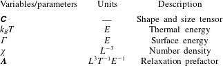
. Table 1 presents the various dimensions associated with the conformation tensor and the four parameters appearing in the model. It should be noted that in the final equations (2.11) and (2.12), only three of these are truly independent:
 $\unicode[STIX]{x1D70F}_{MMG},\unicode[STIX]{x1D709}$
and the product
 $\unicode[STIX]{x1D712}\unicode[STIX]{x1D6E4}$
. The free energy expression in (2.6), through the surface energy term, identifies the surface area with the second invariant of the conformation tensor. As noted before, in comparing the MMG model with the MM model, the main issue with the MMG model is that its conformation tensor is physically identified with the square root of the contravariant tensor describing an ellipsoid, and therefore its reversible dynamics cannot be described by a Poisson structure. Therefore, we consider this model to be both phenomenological and thermodynamically inconsistent in the context of
 $\unicode[STIX]{x1D63E}$
representing an ellipsoid.
Summary of dimensional parameters entering the model:
 $E=\text{energy}$
,
 $L=\text{length}$
and
 $T=\text{time}$
.

From a mathematical point of view, comparing (2.11) with (2.2) also reveals other differences between the two models. Although both models incorporate a nonlinear relaxation term that depends on the invariants, the MMG model possesses an additional nonlinear term proportional to
 $\unicode[STIX]{x1D63E}\unicode[STIX]{x1D63E}$
. There are also similarities between the two models. First, in both models, the dimensionless conformation tensor,
 $\unicode[STIX]{x1D63E}$
, is subject to the constraint
 $I_{3}=1$
, which means that the equilibrium state is identified with
 $\unicode[STIX]{x1D63E}=\unicode[STIX]{x1D739}$
. Second, it is clear that the evolution equations for the conformation tensor in both models have two macroscopic parameters,
 $\unicode[STIX]{x1D709}$
and
 $\unicode[STIX]{x1D70F}$
, the first dimensionless and the second with units of time. An additional benefit of the NET framework underlying the MMG model is the stress tensor that arises self-consistently, a feature absent in the original phenomenological MM model.
The discussion so far has revealed important limitations in both the MM and MMG models, providing justification for the development of improved ellipsoid morphology models. Furthermore, since we seek to describe the general development of a TCEE model, with the key novelty being the exploitation of previous asymptotic results for suspension stress, these are first described before we move on to discuss the development of a TCEE model.
2.3 Asymptotic results from the literature
Microscopic calculations by Schowalter et al. (Reference Schowalter, Chaffey and Brenner1968) and Frankel & Acrivos (Reference Frankel and Acrivos1970), for the rheology of dilute emulsion drops in the absence of inertia, provide the asymptotic results for the effect of drop deformation on the rheology. Drop deformation leads to non-Newtonian rheology at large capillary numbers
 $(Ca)$
, where
 $Ca\equiv \unicode[STIX]{x1D707}a\dot{\unicode[STIX]{x1D6FE}}/T$
, and to
 $O((Ca^{\ast })^{2})$
(where
 $Ca^{\ast }\equiv \unicode[STIX]{x1D707}a/T$
is the interfacial relaxation time), the stress in such an emulsion in a linear flow field is given by the results of Schowalter et al. (Reference Schowalter, Chaffey and Brenner1968) as
 $$\begin{eqnarray}\displaystyle \unicode[STIX]{x1D748} & = & \displaystyle 2\unicode[STIX]{x1D707}\left(1+\unicode[STIX]{x1D719}\left(\frac{5\unicode[STIX]{x1D706}+2}{2(\unicode[STIX]{x1D706}+1)}\right)\right)\unicode[STIX]{x1D63F}-\unicode[STIX]{x1D719}Ca^{\ast }\unicode[STIX]{x1D707}\nonumber\\ \displaystyle & & \displaystyle \times \,\left\{\begin{array}{@{}l@{}}\displaystyle \frac{1}{40}\left(\frac{19\unicode[STIX]{x1D706}+16}{\unicode[STIX]{x1D706}+1}\right)^{2}\left(\frac{\text{D}}{\text{D}t}\unicode[STIX]{x1D63F}-(\unicode[STIX]{x1D734}\boldsymbol{\cdot }\unicode[STIX]{x1D63F}-\unicode[STIX]{x1D63F}\boldsymbol{\cdot }\unicode[STIX]{x1D734})\right)\\ \displaystyle \quad -\,\frac{3(19\unicode[STIX]{x1D706}+16)(25\unicode[STIX]{x1D706}^{2}+41\unicode[STIX]{x1D706}+4)}{140(\unicode[STIX]{x1D706}+1)^{3}}\left(\unicode[STIX]{x1D63F}\boldsymbol{\cdot }\unicode[STIX]{x1D63F}-\frac{1}{3}\text{tr}(\unicode[STIX]{x1D63F}\boldsymbol{\cdot }\unicode[STIX]{x1D63F})\unicode[STIX]{x1D644}\right)\end{array}\right\}+O(Ca^{\ast 2}).\nonumber\\ \displaystyle & & \displaystyle\end{eqnarray}$$
The zeroth-order contribution to the suspension stress is due to the presence of emulsion droplets and solely influences the effective Newtonian viscosity, as was first presented by Taylor (Reference Taylor1932). As seen from (2.13), the
 $O(Ca^{\ast })$
effects ultimately couple nonlinearly to the imposed velocity gradient. Therefore, in addition to thermodynamic consistency, the resultant model we seek to develop should also be able to reproduce the functional dependences present in the asymptotic solution in (2.13), which is derived from microscopic considerations.
3 General development of a TCEE model
The systematic development of a thermodynamically consistent conformation-tensor-based dilute emulsion model is revisited with four main goals in mind: (1) to clarify the nature and physical interpretation of the allowed microstructural variable
 $\unicode[STIX]{x1D63E}$
with relation to idealized reversible dynamics, (2) to understand the role of the approximation inherent in the underlying free energy expression, (3) to understand how the macroscopic parameters entering the model equations may be evaluated while at the same time ensuring consistency with asymptotic results provided by (2.13) and (4) to ensure the proper implementation of the volume conservation constraint through the determinant.
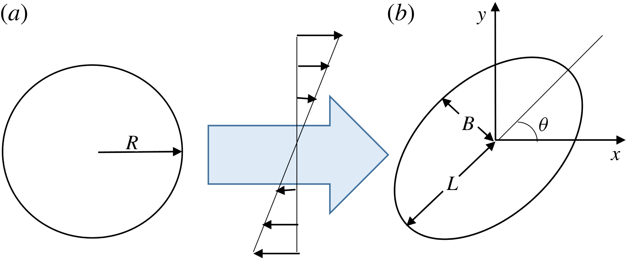
Representation of an equilibrium emulsion droplet (a) and the effect of a shear field in deforming the droplet into an ellipsoidal droplet (b), showing the various geometric parameters when projected in the
 $x$
–
 $y$
plane (plane of shear).

3.1 Selection of the conformation tensor variable
The development of the conformation tensor model begins by making the connection between the internal dimensional conformation tensor variable,
 $\tilde{\unicode[STIX]{x1D63E}}$
, and the canonical representation of the ellipsoid shown in figure 1. The canonical representation of an ellipsoid is given by
 $$\begin{eqnarray}\frac{\tilde{x}_{e}^{2}}{L^{2}}+\frac{{\tilde{y}}_{e}^{2}}{B^{2}}+\frac{\tilde{z}_{e}^{2}}{W^{2}}=1,\end{eqnarray}$$
where
 $L$
,
 $B$
and
 $W$
are the principal semi-axes of the ellipsoid and
 $[\tilde{x}_{e}\;\;{\tilde{y}}_{e}\;\;\tilde{z}_{e}]\equiv \tilde{\boldsymbol{r}}_{e}$
are the dimensional coordinates of a point at the surface of the ellipsoid in a coordinate system constructed along the direction of the axes of the ellipsoid from its centre. Through a similarity transformation, we can express the same relationship in a general coordinate system
 $(x\;\;y\;\;z)$
in tensorial notation as
 $$\begin{eqnarray}\tilde{\unicode[STIX]{x1D60A}}_{ij}^{-1}\tilde{r}_{i}\tilde{r}_{j}=\tilde{\boldsymbol{r}}^{\text{T}}\boldsymbol{\cdot }\tilde{\unicode[STIX]{x1D63E}}^{-1}\boldsymbol{\cdot }\tilde{\boldsymbol{r}}=1,\end{eqnarray}$$
where
 $\tilde{\boldsymbol{r}}=[\tilde{x},{\tilde{y}},\tilde{z}]$
is the dimensional position vector of any point on the ellipsoid surface, with
 $\tilde{\unicode[STIX]{x1D63E}}$
identified through the similarity transformation with a second-order symmetric positive definite tensor with eigenvalues and eigenvectors that are the square of the magnitude and the direction of the semi-axes of the ellipsoid respectively. For dimensional consistency, it follows from (3.2) that
 $\tilde{\unicode[STIX]{x1D63E}}$
has units of length squared. If we now construct the corresponding dimensionless tensor
 $\unicode[STIX]{x1D63E}$
, where
 $\unicode[STIX]{x1D63E}\equiv (1/R^{2})\tilde{\unicode[STIX]{x1D63E}}$
(made dimensionless by the equilibrium droplet radius, see figure 1), then (3.2) transforms to the following equivalent quadratic form:
 $$\begin{eqnarray}r^{\text{T}}\boldsymbol{\cdot }\unicode[STIX]{x1D63E}^{-1}\boldsymbol{\cdot }\boldsymbol{r}=1,\end{eqnarray}$$
where
 $\boldsymbol{r}\equiv \tilde{\boldsymbol{r}}/R$
is the dimensionless position vector of any point on the ellipsoid surface. It should be noted that consistently we recover from (3.3) the equation for a unit sphere as
 $$\begin{eqnarray}r^{\text{T}}\boldsymbol{\cdot }\unicode[STIX]{x1D644}\boldsymbol{\cdot }\boldsymbol{r}=1,\end{eqnarray}$$
characterizing the static (equilibrium) conditions of a droplet at zero deformation with
 $\unicode[STIX]{x1D63E}=\unicode[STIX]{x1D63E}_{equil}=\unicode[STIX]{x1D644}$
and
 $\unicode[STIX]{x1D644}$
the identity tensor. This interpretation of the dimensionless conformation tensor
 $\unicode[STIX]{x1D63E}$
properly identifies it with the tensor used in the MM model by Maffettone & Minale (Reference Maffettone and Minale1998). The significance of this interpretation is that it allows us, as we show immediately below, to determine the proper tensorial nature of
 $\unicode[STIX]{x1D63E}$
as revealed upon the application of an infinitesimal reversible affine material deformation, thereby allowing for the selection of the correct Poisson bracket descriptor of its reversible dynamics.
From the theory of elasticity, for an ideal ellipsoid (as obtained at zero interfacial tension and for a viscosity ratio of one) that deforms affinely with the flow field, and for an infinitesimal deformation, it is the Cauchy strain tensor that provides the correct co-deformational characteristics which describe how points on the boundary of the ellipsoid move. This tensor is the product of the Finger tensor with its transpose, i.e.
 $\unicode[STIX]{x1D63E}=\unicode[STIX]{x1D641}\unicode[STIX]{x1D641}^{\text{T}}$
, with
 $\unicode[STIX]{x1D60D}_{ij}\equiv \unicode[STIX]{x2202}r_{i}^{\prime }/\unicode[STIX]{x2202}r_{j}$
the Finger strain tensor connecting the deformed (primed) and initial (undeformed) spatial coordinates. As a consequence of this definition and following an infinitesimal deformation
 $\boldsymbol{r}\rightarrow \boldsymbol{r}^{\prime }$
, we have
 $$\begin{eqnarray}\boldsymbol{r}^{\prime }=\unicode[STIX]{x1D641}\boldsymbol{\cdot }\boldsymbol{r},\quad \text{infinitesimal deformation}.\end{eqnarray}$$
Let us now assume that we start from an initially undeformed spherical droplet, with a (dimensionless) radius of unity. Consequently, every point,
 $\boldsymbol{r}$
, of the droplet surface obeys the previously mentioned (3.4), corresponding (consistently) to
 $\unicode[STIX]{x1D63E}=\unicode[STIX]{x1D63E}_{equil}=\unicode[STIX]{x1D644}$
. On the other hand, upon an infinitesimal deformation
 $\boldsymbol{r}\rightarrow \boldsymbol{r}^{\prime }$
, the sphere transforms to an ellipsoidal droplet, with any point
 $\boldsymbol{r}^{\prime }$
on its surface obeying (from (3.3))
 $$\begin{eqnarray}\boldsymbol{r}^{\prime \text{T}}\boldsymbol{\cdot }\unicode[STIX]{x1D63E}^{-1}\boldsymbol{\cdot }\boldsymbol{r}^{\prime }=1,\quad \text{deformed }\text{ellipsoidal }\text{droplet}.\end{eqnarray}$$
Substitution of (3.5) into (3.6) leads to
 $$\begin{eqnarray}(\unicode[STIX]{x1D641}\boldsymbol{\cdot }\boldsymbol{r})^{\text{T}}\boldsymbol{\cdot }\unicode[STIX]{x1D63E}^{-1}\boldsymbol{\cdot }(\unicode[STIX]{x1D641}\boldsymbol{\cdot }\boldsymbol{r})=1\Leftrightarrow \boldsymbol{r}^{\text{T}}\boldsymbol{\cdot }\unicode[STIX]{x1D641}^{\text{T}}\boldsymbol{\cdot }\unicode[STIX]{x1D63E}^{-1}\boldsymbol{\cdot }\unicode[STIX]{x1D641}\boldsymbol{\cdot }\boldsymbol{r}=1,\quad \text{deformed }\text{ellipsoidal }\text{droplet},\end{eqnarray}$$
which is expressed now in terms of the position vector
 $\boldsymbol{r}$
of the surface of the undeformed original droplet. However, any such point is known by definition to obey the unity sphere surface definition, (3.4), to which, therefore, (3.7) must be equivalent. Direct comparison of these two equations leads therefore to the equality
 $$\begin{eqnarray}\unicode[STIX]{x1D641}^{\text{T}}\boldsymbol{\cdot }\unicode[STIX]{x1D63E}^{-1}\boldsymbol{\cdot }\unicode[STIX]{x1D641}=\unicode[STIX]{x1D644}\Leftrightarrow \unicode[STIX]{x1D641}^{\text{T}}=(\unicode[STIX]{x1D63E}^{-1}\boldsymbol{\cdot }\unicode[STIX]{x1D641})^{-1}=\unicode[STIX]{x1D641}^{-1}\boldsymbol{\cdot }\unicode[STIX]{x1D63E}\Leftrightarrow \unicode[STIX]{x1D63E}=\unicode[STIX]{x1D641}\boldsymbol{\cdot }\unicode[STIX]{x1D641}^{\text{T}},\end{eqnarray}$$
thus making equivalent the conformation tensor
 $\unicode[STIX]{x1D63E}$
, for this infinitesimal reversible deformation, to the Cauchy strain tensor,
 $\unicode[STIX]{x1D641}\boldsymbol{\cdot }\unicode[STIX]{x1D641}^{\text{T}}$
. However, as shown in ch. 5 of Beris & Edwards (Reference Beris and Edwards1994), the dynamics of the Cauchy strain tensor under flow is provided by the upper-convected time derivative, consistent with the contravariant character of the Cauchy tensor. This therefore proves that the conformation tensor
 $\unicode[STIX]{x1D63E}$
defined in this way is also contravariant and that its reversible dynamics, also described by an upper-convected derivative, can be generated by the same Poisson structure as was developed in ch. 5 of Beris & Edwards (Reference Beris and Edwards1994) for contravariant tensor dynamics.
Alternatively, in a similar fashion, we can also show that
 $\unicode[STIX]{x1D63E}^{-1}$
is covariant in character and that its dynamics can also be described by a Poisson bracket that gives rise to the lower-convected time derivative. It should be noted that these are the only two power forms of
 $\unicode[STIX]{x1D63E}$
, i.e.
 $\unicode[STIX]{x1D63E}^{p}$
with
 $p=1$
or
 $-$
1, that possess a Poisson bracket structure. For any other power law coefficient
 $p$
, the dynamics of the tensor
 $\unicode[STIX]{x1D63E}^{p}$
cannot be expressed solely in terms of the same tensor, thus precluding its direct description through a Poisson bracket, or, equivalently, its usage as a primitive internal variable within a non-equilibrium, bracket formulation, thermodynamics description. Furthermore, this interpretation of the nature of the primitive conformation tensor to be used to describe a deformed ellipsoidal model droplet enforces strict restrictions on the relationship between the surface area of the ellipsoid (and therefore its surface energy) and its evaluation based on the invariants or eigenvalues of
 $\unicode[STIX]{x1D63E}$
, providing further evidence as to why the MMG model is not thermodynamically consistent.
Once the proper tensorial character (i.e. contravariant or covariant nature) of the internal conformation tensor is identified, its Poisson bracket and therefore its reversible dynamics are also in principle fully determined. However, this is true for an unconstrained conformation tensor, such as that used, for example, in describing polymer dynamics (Beris & Edwards Reference Beris and Edwards1994). In the present case, the constraint of unit determinant needs to be properly taken into account. As it turns out, this modifies all subsequent structure (i.e. both the reversible as well as the irreversible dynamics), as explained in detail in § 3.2 below. Once the general equations have been described generically in that subsection in terms of the free energy and the dissipation bracket kernel expressions, the specific choices that we consider as most appropriate to describe the flow dynamics of a dilute emulsion are presented in §§ 3.3–3.5, eventually enabling us to fully define the proposed model. In the last two subsections, §§ 3.6 and 3.7, the proposed model is validated by contrasting its predictions to those independently developed through microscopic analysis around a deformable droplet in the asymptotic limit of small capillary numbers. This comparison allows us, simultaneously to the model validation, to also determine uniquely all of the model parameters.
3.2 Development of the governing equations for a constrained contravariant tensor-based model through the bracket formulation
A constant-volume droplet may be described by a conformation tensor with a constant determinant, which upon suitable rescaling can be equated, for simplicity, to unity, without loss of generality. The introduction of such microstructural constraints must be implemented at the bracket level to ensure that the resulting equations are consistent with the constraints (Edwards et al.
Reference Edwards, Dressler, Grmela and Ait-Kadi2003). For completeness, we repeat the essential components of such a development. Following Edwards et al. (Reference Edwards, Dressler, Grmela and Ait-Kadi2003), the appropriate transformation from an unconstrained
 $\unicode[STIX]{x1D666}$
tensor to a unit determinant constrained
 $\unicode[STIX]{x1D63E}$
tensor is given by
 $$\begin{eqnarray}\unicode[STIX]{x1D666}\rightarrow \unicode[STIX]{x1D63E}=\frac{\unicode[STIX]{x1D666}}{(\det (\unicode[STIX]{x1D666}))^{1/3}}.\end{eqnarray}$$
This relationship can also be inverted to
 $$\begin{eqnarray}\unicode[STIX]{x1D63E}^{-1}=\unicode[STIX]{x1D666}^{-1}(\det (\unicode[STIX]{x1D666}))^{1/3}.\end{eqnarray}$$
Based on these transformations, the Volterra derivative of any functional
 $F$
with respect to the unconstrained conformation tensor
 $\unicode[STIX]{x1D666}$
may be expressed in terms of the Volterra derivative with respect to the constrained conformation tensor
 $\unicode[STIX]{x1D63E}$
as
 $$\begin{eqnarray}\displaystyle \frac{\unicode[STIX]{x1D6FF}F}{\unicode[STIX]{x1D6FF}\unicode[STIX]{x1D632}_{\unicode[STIX]{x1D6FC}\unicode[STIX]{x1D6FD}}} & = & \displaystyle \frac{\unicode[STIX]{x1D6FF}F}{\unicode[STIX]{x1D6FF}\unicode[STIX]{x1D60A}_{\unicode[STIX]{x1D6FE}\unicode[STIX]{x1D700}}}\frac{\unicode[STIX]{x1D6FF}\unicode[STIX]{x1D60A}_{\unicode[STIX]{x1D6FE}\unicode[STIX]{x1D700}}}{\unicode[STIX]{x1D6FF}\unicode[STIX]{x1D632}_{\unicode[STIX]{x1D6FC}\unicode[STIX]{x1D6FD}}}=\frac{1}{(\det \unicode[STIX]{x1D666})^{1/3}}\frac{\unicode[STIX]{x1D6FF}F}{\unicode[STIX]{x1D6FF}\unicode[STIX]{x1D60A}_{\unicode[STIX]{x1D6FE}\unicode[STIX]{x1D700}}}\left(\unicode[STIX]{x1D6FF}_{\unicode[STIX]{x1D6FC}\unicode[STIX]{x1D6FE}}\unicode[STIX]{x1D6FF}_{\unicode[STIX]{x1D6FD}\unicode[STIX]{x1D700}}-\frac{1}{3}\unicode[STIX]{x1D60A}_{\unicode[STIX]{x1D6FE}\unicode[STIX]{x1D700}}\unicode[STIX]{x1D60A}_{\unicode[STIX]{x1D6FC}\unicode[STIX]{x1D6FD}}^{-1}\right)\nonumber\\ \displaystyle & = & \displaystyle \frac{\unicode[STIX]{x1D6FF}F}{\unicode[STIX]{x1D6FF}\unicode[STIX]{x1D60A}_{\unicode[STIX]{x1D6FE}\unicode[STIX]{x1D700}}}\left(\unicode[STIX]{x1D6FF}_{\unicode[STIX]{x1D6FC}\unicode[STIX]{x1D6FE}}\unicode[STIX]{x1D6FF}_{\unicode[STIX]{x1D6FD}\unicode[STIX]{x1D700}}-\frac{1}{3}\unicode[STIX]{x1D60A}_{\unicode[STIX]{x1D6FE}\unicode[STIX]{x1D700}}\unicode[STIX]{x1D60A}_{\unicode[STIX]{x1D6FC}\unicode[STIX]{x1D6FD}}^{-1}\right),\end{eqnarray}$$
with the last equality obtained by exploiting the fact that in the end
 $\unicode[STIX]{x1D666}$
can be set equal to
 $\unicode[STIX]{x1D63E}$
and therefore the determinant of
 $\unicode[STIX]{x1D666}$
can be taken as unity. It should be noted that the Einstein summation convention is followed over repeated indices.
The Poisson bracket developed for an unconstrained conformation tensor
 $\unicode[STIX]{x1D666}$
in Beris & Edwards (Reference Beris and Edwards1994, pp. 217–218), along with the momentum density
 $\boldsymbol{u}$
and the mass density
 $\unicode[STIX]{x1D70C}$
as internal variables, can now be re-expressed using (3.11) for the corresponding Poisson and dissipative bracket structures for a constrained single conformation contravariant tensor,
 $\unicode[STIX]{x1D63E}$
. The key point is that the transformation from the unconstrained brackets to determinant constrained brackets proceeds by replacing all Volterra derivatives with respect to
 $\unicode[STIX]{x1D63E}$
in the former through (3.11). This approach guarantees that the final expressions satisfy the Jacobi identity. Subsequently, the constrained Poisson bracket becomes
 $$\begin{eqnarray}\displaystyle \{F,H\} & = & \displaystyle -\int \left[\frac{\unicode[STIX]{x1D6FF}F}{\unicode[STIX]{x1D6FF}u_{\unicode[STIX]{x1D6FE}}}\unicode[STIX]{x1D735}_{\unicode[STIX]{x1D6FD}}\left(\frac{\unicode[STIX]{x1D6FF}H}{\unicode[STIX]{x1D6FF}u_{\unicode[STIX]{x1D6FD}}}u_{\unicode[STIX]{x1D6FE}}\right)-\frac{\unicode[STIX]{x1D6FF}H}{\unicode[STIX]{x1D6FF}u_{\unicode[STIX]{x1D6FE}}}\unicode[STIX]{x1D735}_{\unicode[STIX]{x1D6FD}}\left(\frac{\unicode[STIX]{x1D6FF}F}{\unicode[STIX]{x1D6FF}u_{\unicode[STIX]{x1D6FD}}}u_{\unicode[STIX]{x1D6FE}}\right)\right]\,\text{d}^{3}r\nonumber\\ \displaystyle & & \displaystyle -\,\int \left[\frac{\unicode[STIX]{x1D6FF}F}{\unicode[STIX]{x1D6FF}\unicode[STIX]{x1D70C}}\unicode[STIX]{x1D735}_{\unicode[STIX]{x1D6FD}}\left(\frac{\unicode[STIX]{x1D6FF}H}{\unicode[STIX]{x1D6FF}u_{\unicode[STIX]{x1D6FD}}}\unicode[STIX]{x1D70C}\right)-\frac{\unicode[STIX]{x1D6FF}H}{\unicode[STIX]{x1D6FF}\unicode[STIX]{x1D70C}}\unicode[STIX]{x1D735}_{\unicode[STIX]{x1D6FD}}\left(\frac{\unicode[STIX]{x1D6FF}F}{\unicode[STIX]{x1D6FF}u_{\unicode[STIX]{x1D6FD}}}\unicode[STIX]{x1D70C}\right)\right]\,\text{d}^{3}r\nonumber\\ \displaystyle & & \displaystyle -\,\int \left[\frac{\unicode[STIX]{x1D6FF}F}{\unicode[STIX]{x1D6FF}\unicode[STIX]{x1D60A}_{\unicode[STIX]{x1D6FC}\unicode[STIX]{x1D6FD}}}\frac{\unicode[STIX]{x1D6FF}H}{\unicode[STIX]{x1D6FF}u_{\unicode[STIX]{x1D6FE}}}\unicode[STIX]{x1D735}_{\unicode[STIX]{x1D6FE}}\unicode[STIX]{x1D60A}_{\unicode[STIX]{x1D6FC}\unicode[STIX]{x1D6FD}}-\frac{\unicode[STIX]{x1D6FF}H}{\unicode[STIX]{x1D6FF}\unicode[STIX]{x1D60A}_{\unicode[STIX]{x1D6FC}\unicode[STIX]{x1D6FD}}}\frac{\unicode[STIX]{x1D6FF}F}{\unicode[STIX]{x1D6FF}u_{\unicode[STIX]{x1D6FE}}}\unicode[STIX]{x1D735}_{\unicode[STIX]{x1D6FE}}\unicode[STIX]{x1D60A}_{\unicode[STIX]{x1D6FC}\unicode[STIX]{x1D6FD}}\right]\,\text{d}^{3}r\nonumber\\ \displaystyle & & \displaystyle +\,\frac{1}{3}\int \unicode[STIX]{x1D60A}_{\unicode[STIX]{x1D6FC}\unicode[STIX]{x1D6FD}}\left[\frac{\unicode[STIX]{x1D6FF}H}{\unicode[STIX]{x1D6FF}\unicode[STIX]{x1D60A}_{\unicode[STIX]{x1D6FC}\unicode[STIX]{x1D6FD}}}\unicode[STIX]{x1D60A}_{\unicode[STIX]{x1D70C}\unicode[STIX]{x1D702}}^{-1}\left(\frac{\unicode[STIX]{x1D6FF}F}{\unicode[STIX]{x1D6FF}u_{\unicode[STIX]{x1D6FE}}}\right)\unicode[STIX]{x1D735}_{\unicode[STIX]{x1D6FE}}\unicode[STIX]{x1D60A}_{\unicode[STIX]{x1D70C}\unicode[STIX]{x1D702}}-\frac{\unicode[STIX]{x1D6FF}F}{\unicode[STIX]{x1D6FF}\unicode[STIX]{x1D60A}_{\unicode[STIX]{x1D6FC}\unicode[STIX]{x1D6FD}}}\unicode[STIX]{x1D60A}_{\unicode[STIX]{x1D70C}\unicode[STIX]{x1D702}}^{-1}\left(\frac{\unicode[STIX]{x1D6FF}H}{\unicode[STIX]{x1D6FF}u_{\unicode[STIX]{x1D6FE}}}\right)\unicode[STIX]{x1D735}_{\unicode[STIX]{x1D6FE}}\unicode[STIX]{x1D60A}_{\unicode[STIX]{x1D70C}\unicode[STIX]{x1D702}}\right]\,\text{d}^{3}r\nonumber\\ \displaystyle & & \displaystyle -\,\int \unicode[STIX]{x1D60A}_{\unicode[STIX]{x1D6FC}\unicode[STIX]{x1D6FE}}\left[\frac{\unicode[STIX]{x1D6FF}H}{\unicode[STIX]{x1D6FF}\unicode[STIX]{x1D60A}_{\unicode[STIX]{x1D6FC}\unicode[STIX]{x1D6FD}}}\unicode[STIX]{x1D735}_{\unicode[STIX]{x1D6FE}}\left(\frac{\unicode[STIX]{x1D6FF}F}{\unicode[STIX]{x1D6FF}u_{\unicode[STIX]{x1D6FD}}}\right)-\frac{\unicode[STIX]{x1D6FF}F}{\unicode[STIX]{x1D6FF}\unicode[STIX]{x1D60A}_{\unicode[STIX]{x1D6FC}\unicode[STIX]{x1D6FD}}}\unicode[STIX]{x1D735}_{\unicode[STIX]{x1D6FE}}\left(\frac{\unicode[STIX]{x1D6FF}H}{\unicode[STIX]{x1D6FF}u_{\unicode[STIX]{x1D6FD}}}\right)\right]\,\text{d}^{3}r\nonumber\\ \displaystyle & & \displaystyle -\,\int \unicode[STIX]{x1D60A}_{\unicode[STIX]{x1D6FD}\unicode[STIX]{x1D6FE}}\left[\frac{\unicode[STIX]{x1D6FF}H}{\unicode[STIX]{x1D6FF}\unicode[STIX]{x1D60A}_{\unicode[STIX]{x1D6FC}\unicode[STIX]{x1D6FD}}}\unicode[STIX]{x1D735}_{\unicode[STIX]{x1D6FE}}\left(\frac{\unicode[STIX]{x1D6FF}F}{\unicode[STIX]{x1D6FF}u_{\unicode[STIX]{x1D6FC}}}\right)-\frac{\unicode[STIX]{x1D6FF}F}{\unicode[STIX]{x1D6FF}\unicode[STIX]{x1D60A}_{\unicode[STIX]{x1D6FC}\unicode[STIX]{x1D6FD}}}\unicode[STIX]{x1D735}_{\unicode[STIX]{x1D6FE}}\left(\frac{\unicode[STIX]{x1D6FF}H}{\unicode[STIX]{x1D6FF}u_{\unicode[STIX]{x1D6FC}}}\right)\right]\,\text{d}^{3}r\nonumber\\ \displaystyle & & \displaystyle +\,\frac{2}{3}\int \unicode[STIX]{x1D60A}_{\unicode[STIX]{x1D6FC}\unicode[STIX]{x1D6FD}}\left[\frac{\unicode[STIX]{x1D6FF}F}{\unicode[STIX]{x1D6FF}\unicode[STIX]{x1D60A}_{\unicode[STIX]{x1D6FC}\unicode[STIX]{x1D6FD}}}\unicode[STIX]{x1D735}_{\unicode[STIX]{x1D6FE}}\left(\frac{\unicode[STIX]{x1D6FF}H}{\unicode[STIX]{x1D6FF}u_{\unicode[STIX]{x1D6FE}}}\right)-\frac{\unicode[STIX]{x1D6FF}H}{\unicode[STIX]{x1D6FF}\unicode[STIX]{x1D60A}_{\unicode[STIX]{x1D6FC}\unicode[STIX]{x1D6FD}}}\unicode[STIX]{x1D735}_{\unicode[STIX]{x1D6FE}}\left(\frac{\unicode[STIX]{x1D6FF}F}{\unicode[STIX]{x1D6FF}u_{\unicode[STIX]{x1D6FE}}}\right)\right]\,\text{d}^{3}r.\end{eqnarray}$$
The effect of the volume constraint is to modify the unconstrained Poisson bracket by introducing terms proportional to
 $1/3$
in (3.12). We note that the fourth term on the right-hand side in this equation was omitted in the expressions given by Edwards et al. (Reference Edwards, Dressler, Grmela and Ait-Kadi2003). A similar form for the Poisson bracket, albeit restricted to incompressible flows, has also been proposed for the development of the MMG model (Grmela et al.
Reference Grmela, Ammar, Chinesta and Maîtrejean2014).
Similarly, the kernel for a general dissipative bracket
 $[F,H]$
, which has been developed as the lowest-order (bilinear) expression in terms of the Volterra derivatives for the unconstrained conformation tensor
 $\unicode[STIX]{x1D666}$
in Beris & Edwards (Reference Beris and Edwards1994, p. 219), is expressed as
 $$\begin{eqnarray}\displaystyle [F,H]_{wec} & = & \displaystyle -\int \unicode[STIX]{x1D6EC}_{\unicode[STIX]{x1D6FC}\unicode[STIX]{x1D6FD}\unicode[STIX]{x1D6FE}\unicode[STIX]{x1D700}}\left(\frac{\unicode[STIX]{x1D6FF}F}{\unicode[STIX]{x1D6FF}\unicode[STIX]{x1D60A}_{\unicode[STIX]{x1D6FC}\unicode[STIX]{x1D6FD}}}\left(\frac{\unicode[STIX]{x1D6FF}H}{\unicode[STIX]{x1D6FF}\unicode[STIX]{x1D60A}_{\unicode[STIX]{x1D6FE}\unicode[STIX]{x1D700}}}-\frac{1}{3}\unicode[STIX]{x1D60A}_{\unicode[STIX]{x1D70C}\unicode[STIX]{x1D702}}\frac{\unicode[STIX]{x1D6FF}H}{\unicode[STIX]{x1D6FF}\unicode[STIX]{x1D60A}_{\unicode[STIX]{x1D70C}\unicode[STIX]{x1D702}}}\unicode[STIX]{x1D60A}_{\unicode[STIX]{x1D6FE}\unicode[STIX]{x1D700}}^{-1}\right)\right.\nonumber\\ \displaystyle & & \displaystyle \left.-\,\frac{1}{3}\unicode[STIX]{x1D60A}_{\unicode[STIX]{x1D70C}\unicode[STIX]{x1D702}}\unicode[STIX]{x1D60A}_{\unicode[STIX]{x1D6FC}\unicode[STIX]{x1D6FD}}^{-1}\frac{\unicode[STIX]{x1D6FF}F}{\unicode[STIX]{x1D6FF}\unicode[STIX]{x1D60A}_{\unicode[STIX]{x1D70C}\unicode[STIX]{x1D702}}}\left(\frac{\unicode[STIX]{x1D6FF}H}{\unicode[STIX]{x1D6FF}\unicode[STIX]{x1D60A}_{\unicode[STIX]{x1D6FE}\unicode[STIX]{x1D700}}}-\frac{1}{3}\unicode[STIX]{x1D60A}_{\unicode[STIX]{x1D70F}\unicode[STIX]{x1D710}}\frac{\unicode[STIX]{x1D6FF}H}{\unicode[STIX]{x1D6FF}\unicode[STIX]{x1D60A}_{\unicode[STIX]{x1D70F}\unicode[STIX]{x1D710}}}\unicode[STIX]{x1D60A}_{\unicode[STIX]{x1D6FE}\unicode[STIX]{x1D700}}^{-1}\right)\right)\,\text{d}^{3}r\nonumber\\ \displaystyle & & \displaystyle -\,\int Q_{\unicode[STIX]{x1D6FC}\unicode[STIX]{x1D6FD}\unicode[STIX]{x1D6FE}\unicode[STIX]{x1D700}}\left(\unicode[STIX]{x1D735}_{\unicode[STIX]{x1D6FC}}\frac{\unicode[STIX]{x1D6FF}F}{\unicode[STIX]{x1D6FF}u_{\unicode[STIX]{x1D6FD}}}\right)\left(\unicode[STIX]{x1D735}_{\unicode[STIX]{x1D6FE}}\frac{\unicode[STIX]{x1D6FF}H}{\unicode[STIX]{x1D6FF}u_{\unicode[STIX]{x1D700}}}\right)\,\text{d}^{3}r\nonumber\\ \displaystyle & & \displaystyle -\,\int L_{\unicode[STIX]{x1D6FC}\unicode[STIX]{x1D6FD}\unicode[STIX]{x1D6FE}\unicode[STIX]{x1D700}}\left(\unicode[STIX]{x1D735}_{\unicode[STIX]{x1D6FC}}\frac{\unicode[STIX]{x1D6FF}F}{\unicode[STIX]{x1D6FF}u_{\unicode[STIX]{x1D6FD}}}\left(\frac{\unicode[STIX]{x1D6FF}H}{\unicode[STIX]{x1D6FF}\unicode[STIX]{x1D60A}_{\unicode[STIX]{x1D6FE}\unicode[STIX]{x1D700}}}-\frac{1}{3}\unicode[STIX]{x1D60A}_{\unicode[STIX]{x1D70C}\unicode[STIX]{x1D702}}\frac{\unicode[STIX]{x1D6FF}H}{\unicode[STIX]{x1D6FF}\unicode[STIX]{x1D632}_{\unicode[STIX]{x1D70C}\unicode[STIX]{x1D702}}}\unicode[STIX]{x1D60A}_{\unicode[STIX]{x1D6FE}\unicode[STIX]{x1D700}}^{-1}\right)-\unicode[STIX]{x1D735}_{\unicode[STIX]{x1D6FC}}\frac{\unicode[STIX]{x1D6FF}H}{\unicode[STIX]{x1D6FF}u_{\unicode[STIX]{x1D6FD}}}\frac{\unicode[STIX]{x1D6FF}F}{\unicode[STIX]{x1D6FF}\unicode[STIX]{x1D60A}_{\unicode[STIX]{x1D6FE}\unicode[STIX]{x1D700}}}\right.\nonumber\\ \displaystyle & & \displaystyle \left.-\,\frac{1}{3}\unicode[STIX]{x1D60A}_{\unicode[STIX]{x1D70C}\unicode[STIX]{x1D702}}\unicode[STIX]{x1D60A}_{\unicode[STIX]{x1D6FE}\unicode[STIX]{x1D700}}^{-1}\unicode[STIX]{x1D735}_{\unicode[STIX]{x1D6FC}}\frac{\unicode[STIX]{x1D6FF}H}{\unicode[STIX]{x1D6FF}u_{\unicode[STIX]{x1D6FD}}}\frac{\unicode[STIX]{x1D6FF}F}{\unicode[STIX]{x1D6FF}\unicode[STIX]{x1D60A}_{\unicode[STIX]{x1D70C}\unicode[STIX]{x1D702}}}\right)\,\text{d}^{3}r,\end{eqnarray}$$
where by kernel, symbolized here with the subscript
 $wec$
, we mean ‘without entropy correction’, i.e. without terms involving derivatives with respect to entropy. Such terms only affect non-isothermal flows, which are not considered here.
In (3.13), we need to further specify
 $L_{\unicode[STIX]{x1D6FC}\unicode[STIX]{x1D6FD}\unicode[STIX]{x1D6FE}\unicode[STIX]{x1D700}}$
using the expression provided in Beris & Edwards (Reference Beris and Edwards1994, p. 226),
 $$\begin{eqnarray}L_{\unicode[STIX]{x1D6FC}\unicode[STIX]{x1D6FD}\unicode[STIX]{x1D6FE}\unicode[STIX]{x1D700}}=-\frac{\unicode[STIX]{x1D709}}{2}(\unicode[STIX]{x1D60A}_{\unicode[STIX]{x1D6FC}\unicode[STIX]{x1D6FE}}\unicode[STIX]{x1D6FF}_{\unicode[STIX]{x1D6FD}\unicode[STIX]{x1D700}}+\unicode[STIX]{x1D60A}_{\unicode[STIX]{x1D6FC}\unicode[STIX]{x1D700}}\unicode[STIX]{x1D6FF}_{\unicode[STIX]{x1D6FD}\unicode[STIX]{x1D6FE}}+\unicode[STIX]{x1D60A}_{\unicode[STIX]{x1D6FD}\unicode[STIX]{x1D6FE}}\unicode[STIX]{x1D6FF}_{\unicode[STIX]{x1D6FC}\unicode[STIX]{x1D700}}+\unicode[STIX]{x1D60A}_{\unicode[STIX]{x1D6FD}\unicode[STIX]{x1D700}}\unicode[STIX]{x1D6FF}_{\unicode[STIX]{x1D6FC}\unicode[STIX]{x1D6FE}}),\end{eqnarray}$$
where
 $\unicode[STIX]{x1D709}$
is the usual non-affine parameter. This form gives rise to the Gordon–Schowalter derivative. The resulting dynamical equation for the constrained conformation tensor
 $\unicode[STIX]{x1D63E}$
is then given from the above Poisson and dissipation brackets following the general practices outlined by Beris & Edwards (Reference Beris and Edwards1994). More specifically, in order to derive the spatial form of the evolution equations for the variables, one uses the expression
 $$\begin{eqnarray}\frac{\text{d}F}{\text{d}t}=\{F,H\}+[F,H]=\int \left(\frac{\unicode[STIX]{x2202}\unicode[STIX]{x1D70C}}{\unicode[STIX]{x2202}t}\frac{\unicode[STIX]{x2202}F}{\unicode[STIX]{x2202}\unicode[STIX]{x1D70C}}+\frac{\unicode[STIX]{x2202}\unicode[STIX]{x1D60A}_{\unicode[STIX]{x1D6FC}\unicode[STIX]{x1D6FD}}}{\unicode[STIX]{x2202}t}\frac{\unicode[STIX]{x2202}F}{\unicode[STIX]{x2202}\unicode[STIX]{x1D60A}_{\unicode[STIX]{x1D6FC}\unicode[STIX]{x1D6FD}}}+\frac{\unicode[STIX]{x2202}u_{\unicode[STIX]{x1D6FC}}}{\unicode[STIX]{x2202}t}\frac{\unicode[STIX]{x2202}F}{\unicode[STIX]{x2202}u_{\unicode[STIX]{x1D6FC}}}\right)\,\text{d}^{3}r,\end{eqnarray}$$
to match against the relevant terms appearing in the Poisson and dissipative brackets, requiring the two expressions to give identical results for arbitrary functionals
 $F$
. This is the same starting point as in the MMG model (Grmela et al.
Reference Grmela, Ammar, Chinesta and Maîtrejean2014), albeit a more specific expression for the dissipation bracket is developed through the dissipation potential (Grmela Reference Grmela1984). In particular, applying (3.15) for
 $\unicode[STIX]{x1D63E}$
contributions leads to the evolution equation for the conformation tensor as
 $$\begin{eqnarray}\displaystyle \frac{\text{D}^{(\unicode[STIX]{x1D709})}\unicode[STIX]{x1D60A}_{\unicode[STIX]{x1D6FC}\unicode[STIX]{x1D6FD}}}{\text{d}t} & = & \displaystyle \frac{2}{3}\unicode[STIX]{x1D709}\unicode[STIX]{x1D60A}_{\unicode[STIX]{x1D6FC}\unicode[STIX]{x1D6FD}}\unicode[STIX]{x1D60B}_{\unicode[STIX]{x1D6FE}\unicode[STIX]{x1D6FE}}-\frac{2}{3}\unicode[STIX]{x1D60A}_{\unicode[STIX]{x1D6FC}\unicode[STIX]{x1D6FD}}\unicode[STIX]{x1D735}_{\unicode[STIX]{x1D6FE}}v_{\unicode[STIX]{x1D6FE}}-\frac{1}{3}\unicode[STIX]{x1D60A}_{\unicode[STIX]{x1D6FC}\unicode[STIX]{x1D6FD}}\unicode[STIX]{x1D60A}_{\unicode[STIX]{x1D70C}\unicode[STIX]{x1D702}}^{-1}v_{\unicode[STIX]{x1D6FE}}\unicode[STIX]{x1D735}_{\unicode[STIX]{x1D6FE}}\unicode[STIX]{x1D60A}_{\unicode[STIX]{x1D70C}\unicode[STIX]{x1D702}}\nonumber\\ \displaystyle & & \displaystyle -\,\unicode[STIX]{x1D6EC}_{\unicode[STIX]{x1D6FC}\unicode[STIX]{x1D6FD}\unicode[STIX]{x1D6FE}\unicode[STIX]{x1D700}}\left(\frac{\unicode[STIX]{x1D6FF}H}{\unicode[STIX]{x1D6FF}\unicode[STIX]{x1D60A}_{\unicode[STIX]{x1D6FE}\unicode[STIX]{x1D700}}}-\frac{1}{3}\unicode[STIX]{x1D60A}_{\unicode[STIX]{x1D70C}\unicode[STIX]{x1D702}}\frac{\unicode[STIX]{x1D6FF}H}{\unicode[STIX]{x1D6FF}\unicode[STIX]{x1D60A}_{\unicode[STIX]{x1D70C}\unicode[STIX]{x1D702}}}\unicode[STIX]{x1D60A}_{\unicode[STIX]{x1D6FE}\unicode[STIX]{x1D700}}^{-1}\right)\nonumber\\ \displaystyle & & \displaystyle +\,\frac{1}{3}\unicode[STIX]{x1D6EC}_{\unicode[STIX]{x1D70C}\unicode[STIX]{x1D702}\unicode[STIX]{x1D6FE}\unicode[STIX]{x1D700}}\unicode[STIX]{x1D60A}_{\unicode[STIX]{x1D70C}\unicode[STIX]{x1D702}}^{-1}\left(\frac{\unicode[STIX]{x1D6FF}H}{\unicode[STIX]{x1D6FF}\unicode[STIX]{x1D60A}_{\unicode[STIX]{x1D6FE}\unicode[STIX]{x1D700}}}-\frac{1}{3}\unicode[STIX]{x1D60A}_{\unicode[STIX]{x1D708}\unicode[STIX]{x1D707}}\frac{\unicode[STIX]{x1D6FF}H}{\unicode[STIX]{x1D6FF}\unicode[STIX]{x1D60A}_{\unicode[STIX]{x1D708}\unicode[STIX]{x1D707}}}\unicode[STIX]{x1D60A}_{\unicode[STIX]{x1D6FE}\unicode[STIX]{x1D700}}^{-1}\right)\unicode[STIX]{x1D60A}_{\unicode[STIX]{x1D6FC}\unicode[STIX]{x1D6FD}}.\end{eqnarray}$$
It is easy to show that
 $\text{D}^{(\unicode[STIX]{x1D709})}(\det (\unicode[STIX]{x1D63E}))/\text{d}t=\unicode[STIX]{x1D60A}_{\unicode[STIX]{x1D6FC}\unicode[STIX]{x1D6FD}}^{-1}((\text{D}^{(\unicode[STIX]{x1D709})}\unicode[STIX]{x1D60A}_{\unicode[STIX]{x1D6FC}\unicode[STIX]{x1D6FD}})/\text{d}t)=0$
, and therefore demonstrate that this evolution equation automatically guarantees the invariance of the determinant of
 $\unicode[STIX]{x1D63E}$
. For incompressible and homogeneous flows, the expression above can be further simplified to
 $$\begin{eqnarray}\displaystyle \frac{\text{D}^{(\unicode[STIX]{x1D709})}\unicode[STIX]{x1D60A}_{\unicode[STIX]{x1D6FC}\unicode[STIX]{x1D6FD}}}{\text{d}t} & = & \displaystyle -\unicode[STIX]{x1D6EC}_{\unicode[STIX]{x1D6FC}\unicode[STIX]{x1D6FD}\unicode[STIX]{x1D6FE}\unicode[STIX]{x1D700}}\left(\frac{\unicode[STIX]{x1D6FF}H}{\unicode[STIX]{x1D6FF}\unicode[STIX]{x1D60A}_{\unicode[STIX]{x1D6FE}\unicode[STIX]{x1D700}}}-\frac{1}{3}\unicode[STIX]{x1D60A}_{\unicode[STIX]{x1D70C}\unicode[STIX]{x1D702}}\frac{\unicode[STIX]{x1D6FF}H}{\unicode[STIX]{x1D6FF}\unicode[STIX]{x1D60A}_{\unicode[STIX]{x1D70C}\unicode[STIX]{x1D702}}}\unicode[STIX]{x1D60A}_{\unicode[STIX]{x1D6FE}\unicode[STIX]{x1D700}}^{-1}\right)\nonumber\\ \displaystyle & & \displaystyle +\,\frac{1}{3}\unicode[STIX]{x1D6EC}_{\unicode[STIX]{x1D70C}\unicode[STIX]{x1D702}\unicode[STIX]{x1D6FE}\unicode[STIX]{x1D700}}\unicode[STIX]{x1D60A}_{\unicode[STIX]{x1D70C}\unicode[STIX]{x1D702}}^{-1}\left(\frac{\unicode[STIX]{x1D6FF}H}{\unicode[STIX]{x1D6FF}\unicode[STIX]{x1D60A}_{\unicode[STIX]{x1D6FE}\unicode[STIX]{x1D700}}}-\frac{1}{3}\unicode[STIX]{x1D60A}_{\unicode[STIX]{x1D708}\unicode[STIX]{x1D707}}\frac{\unicode[STIX]{x1D6FF}H}{\unicode[STIX]{x1D6FF}\unicode[STIX]{x1D60A}_{\unicode[STIX]{x1D708}\unicode[STIX]{x1D707}}}\unicode[STIX]{x1D60A}_{\unicode[STIX]{x1D6FE}\unicode[STIX]{x1D700}}^{-1}\right)\unicode[STIX]{x1D60A}_{\unicode[STIX]{x1D6FC}\unicode[STIX]{x1D6FD}}.\end{eqnarray}$$
In addition, the corresponding stress expression is given by
 $$\begin{eqnarray}\unicode[STIX]{x1D70E}_{\unicode[STIX]{x1D6FC}\unicode[STIX]{x1D6FD}}=Q_{\unicode[STIX]{x1D6FC}\unicode[STIX]{x1D6FD}\unicode[STIX]{x1D6FE}\unicode[STIX]{x1D700}}\unicode[STIX]{x1D735}_{\unicode[STIX]{x1D6FE}}v_{\unicode[STIX]{x1D700}}+2(1-\unicode[STIX]{x1D709})\unicode[STIX]{x1D60A}_{\unicode[STIX]{x1D6FD}\unicode[STIX]{x1D6FE}}\frac{\unicode[STIX]{x1D6FF}H}{\unicode[STIX]{x1D6FF}\unicode[STIX]{x1D60A}_{\unicode[STIX]{x1D6FC}\unicode[STIX]{x1D6FE}}}-\frac{2}{3}(1-\unicode[STIX]{x1D709})\unicode[STIX]{x1D60A}_{\unicode[STIX]{x1D70C}\unicode[STIX]{x1D700}}\frac{\unicode[STIX]{x1D6FF}H}{\unicode[STIX]{x1D6FF}\unicode[STIX]{x1D60A}_{\unicode[STIX]{x1D70C}\unicode[STIX]{x1D700}}}\unicode[STIX]{x1D6FF}_{\unicode[STIX]{x1D6FC}\unicode[STIX]{x1D6FD}}.\end{eqnarray}$$
The effect of the volume constraint is to introduce some new terms in the model, so that the constraint
 $\text{D}^{(\unicode[STIX]{x1D709})}(\det (\unicode[STIX]{x1D63E}))/\text{d}t=0$
is duly satisfied under all circumstances. The expressions derived so far in (3.16)–(3.18) describe the time derivative of
 $\unicode[STIX]{x1D63E}$
and the stress tensor
 $\unicode[STIX]{x1D748}$
. However, to proceed further, it is necessary to specify the form of the free energy,
 $H$
, the fourth-order viscosity matrix
 $Q_{\unicode[STIX]{x1D6FC}\unicode[STIX]{x1D6FD}\unicode[STIX]{x1D6FE}\unicode[STIX]{x1D700}}$
as well as the fourth-order relaxation tensor
 $\unicode[STIX]{x1D6EC}_{\unicode[STIX]{x1D70C}\unicode[STIX]{x1D702}\unicode[STIX]{x1D6FE}\unicode[STIX]{x1D700}}$
. Whereas for
 $H$
one can use the underlying physics, no particular guidance exists for choosing the latter two. The approach taken in this work is to make these selections such that we can consistently recover a general functional form comparable to the asymptotic solutions of the microscopic flow around isolated ellipsoidal droplets to second order in capillary number, as shown in § 2.3. The next section focuses on examining the impact of the approximation used for the free energy expression as well as the various formulae chosen to represent the fourth-order tensors that allow us to achieve the aforementioned objective.
3.3 The free energy expression
From continuum mechanics, the general dependence of a scalar, the internal energy, in terms of a tensor
 $\unicode[STIX]{x1D63E}$
can be expressed by the following volume integral:
 $$\begin{eqnarray}E=\int g(I_{1},I_{2})\,\text{d}V.\end{eqnarray}$$
In general, the internal energy density
 $g$
depends on all of the invariants of the conformation tensor
 $\unicode[STIX]{x1D63E}$
. However, here it is only given as a function of the first two invariants since the third is constrained to be always 1. Beyond that, it has to best express the relevant physics. For emulsions, the internal energy is the interfacial energy of the droplets, and therefore
 $g$
is taken to be equal to
 $N_{D}\unicode[STIX]{x1D6FE}S_{D}$
, where
 $N_{D}$
is the number density of the droplets,
 $\unicode[STIX]{x1D6FE}$
is the surface tension and
 $S_{D}$
is the surface area of each droplet. If no breakage or coalescence is assumed, the number density of droplets,
 $N_{D}$
, is considered to be constant. In turn,
 $S_{D}$
is expressed as a product of the area of the equilibrium droplet (
 $4\unicode[STIX]{x03C0}R^{2}$
) and a dimensionless area
 $h(I_{1},I_{2})$
, to be specified later. Thus,
 $$\begin{eqnarray}g(I_{1},I_{2})=\unicode[STIX]{x1D719}\unicode[STIX]{x1D6E4}h(I_{1},I_{2}),\end{eqnarray}$$
where
 $\unicode[STIX]{x1D6E4}\equiv 3\unicode[STIX]{x1D6FE}/R$
is the surface energy density,
 $R$
is the radius of the spherical droplet at equilibrium and
 $\unicode[STIX]{x1D719}$
is the volume fraction of the dispersed emulsion droplets. In this expression,
 $h(I_{1},I_{2})$
accounts for changes in area due to droplet deformation, and, for consistency, at equilibrium,
 $h(I_{1},I_{2})=1$
.
The expression for the entropy of mixing functional,
 $S_{m}$
, is given by
 $$\begin{eqnarray}S_{m}=\int s_{m}(\unicode[STIX]{x1D719})\,\text{d}\boldsymbol{r},\end{eqnarray}$$
where
 $s(\unicode[STIX]{x1D719})$
is the entropy density which is a function of the volume fraction. This leads to the final complete expression for the Hamiltonian in terms of the constrained variable,
 $\unicode[STIX]{x1D63E}$
, which is given by
 $$\begin{eqnarray}H=\int \left(\frac{\frac{1}{2}\boldsymbol{u}^{2}}{\unicode[STIX]{x1D70C}}+g(I_{1},I_{2})+h_{s}(T)s_{m}(\unicode[STIX]{x1D719})\right)\,\text{d}\boldsymbol{r},\end{eqnarray}$$
where
 $h_{s}(T)$
is a free energy contribution from the solvent. It should be noted that for a homogeneous isothermal system in which the volume fraction and temperature are constant such as that being considered here, the particular forms of
 $s_{m}(\unicode[STIX]{x1D719})$
and
 $h_{s}(T)$
are neither of concern nor necessary inputs in the discussion and analysis that follows, and can safely be ignored.
The Volterra derivative of the free energy in (3.22) which belongs in the same vector subspace as the partial derivatives of the conformation tensor
 $\unicode[STIX]{x1D63E}$
is defined by
 $$\begin{eqnarray}\frac{\unicode[STIX]{x1D6FF}H}{\unicode[STIX]{x1D6FF}\unicode[STIX]{x1D60A}_{\unicode[STIX]{x1D6FC}\unicode[STIX]{x1D6FD}}}=\unicode[STIX]{x1D6F1}_{\unicode[STIX]{x1D6FC}\unicode[STIX]{x1D6FD}\unicode[STIX]{x1D6FE}\unicode[STIX]{x1D700}}\frac{\unicode[STIX]{x2202}g}{\unicode[STIX]{x2202}\unicode[STIX]{x1D60A}_{\unicode[STIX]{x1D6FE}\unicode[STIX]{x1D700}}},\end{eqnarray}$$
where the projector operator
 $\unicode[STIX]{x1D6F1}_{\unicode[STIX]{x1D6FC}\unicode[STIX]{x1D6FD}\unicode[STIX]{x1D6FE}\unicode[STIX]{x1D700}}$
for a system subject to a constraint
 $\det (\unicode[STIX]{x1D63E})=1$
is given by
 $$\begin{eqnarray}\unicode[STIX]{x1D6F1}_{\unicode[STIX]{x1D6FC}\unicode[STIX]{x1D6FD}\unicode[STIX]{x1D6FE}\unicode[STIX]{x1D700}}=\unicode[STIX]{x1D6FF}_{\unicode[STIX]{x1D6FC}\unicode[STIX]{x1D6FE}}\unicode[STIX]{x1D6FF}_{\unicode[STIX]{x1D6FD}\unicode[STIX]{x1D700}}-\left(\frac{\unicode[STIX]{x1D60A}_{\unicode[STIX]{x1D6FE}\unicode[STIX]{x1D700}}^{-1}}{\unicode[STIX]{x1D60A}_{\unicode[STIX]{x1D6FE}\unicode[STIX]{x1D700}}^{-1}\unicode[STIX]{x1D60A}_{\unicode[STIX]{x1D6FE}\unicode[STIX]{x1D700}}^{-1}}\right)\unicode[STIX]{x1D60A}_{\unicode[STIX]{x1D6FC}\unicode[STIX]{x1D6FD}}^{-1}.\end{eqnarray}$$
The derivation of this projector operator is provided in appendix A. The partial derivative of
 $g$
corresponding to the definition in (3.20) is given by
 $$\begin{eqnarray}\frac{\unicode[STIX]{x2202}g}{\unicode[STIX]{x2202}\unicode[STIX]{x1D60A}_{\unicode[STIX]{x1D6FE}\unicode[STIX]{x1D700}}}=\unicode[STIX]{x1D719}\unicode[STIX]{x1D6E4}((\unicode[STIX]{x2202}h/\unicode[STIX]{x2202}I_{1})(\unicode[STIX]{x1D6FF}_{\unicode[STIX]{x1D6FE}\unicode[STIX]{x1D700}})+(\unicode[STIX]{x2202}h/\unicode[STIX]{x2202}I_{2})(I_{1}\unicode[STIX]{x1D6FF}_{\unicode[STIX]{x1D6FE}\unicode[STIX]{x1D700}}-\unicode[STIX]{x1D60A}_{\unicode[STIX]{x1D6FE}\unicode[STIX]{x1D700}})).\end{eqnarray}$$
Consequently, the Volterra derivative of the free energy in the determinant-constrained subspace is given by
 $$\begin{eqnarray}\displaystyle \frac{\unicode[STIX]{x1D6FF}H}{\unicode[STIX]{x1D6FF}\unicode[STIX]{x1D60A}_{\unicode[STIX]{x1D6FE}\unicode[STIX]{x1D700}}} & = & \displaystyle \unicode[STIX]{x1D719}\unicode[STIX]{x1D6E4}\left((\unicode[STIX]{x2202}h/\unicode[STIX]{x2202}I_{1})\left(\unicode[STIX]{x1D6FF}_{\unicode[STIX]{x1D6FE}\unicode[STIX]{x1D700}}-\left(\frac{I_{2}}{I_{2}^{2}-2I_{1}}\right)\unicode[STIX]{x1D60A}_{\unicode[STIX]{x1D6FE}\unicode[STIX]{x1D700}}^{-1}\right)\right.\nonumber\\ \displaystyle & & \displaystyle \left.+\,(\unicode[STIX]{x2202}h/\unicode[STIX]{x2202}I_{2})\left(I_{1}\unicode[STIX]{x1D6FF}_{\unicode[STIX]{x1D6FE}\unicode[STIX]{x1D700}}-\unicode[STIX]{x1D60A}_{\unicode[STIX]{x1D6FE}\unicode[STIX]{x1D700}}-\left(\frac{I_{1}I_{2}-3}{I_{2}^{2}-2I_{1}}\right)\unicode[STIX]{x1D60A}_{\unicode[STIX]{x1D6FE}\unicode[STIX]{x1D700}}^{-1}\right)\right).\end{eqnarray}$$
It is noteworthy that this expression does not involve the entropic contribution to the free energy i.e. only the partial derivative of the interfacial free energy appears. This is physically meaningful since the entropy function only depends on the volume fraction and not on the shape of the ellipsoidal particles.
To make further progress, a specific expression for the normalized shape function is needed. Ideally, this should represent the surface of a general (tri-axial) ellipsoid whose axes are represented by the eigenvalues/eigenvectors of the conformation tensor
 $\unicode[STIX]{x1D63E}$
. However, an exact expression is difficult to obtain for the general case. Therefore, we propose to use Knud Thomsen’s approximation (Xu et al.
Reference Xu, Cui, Bansal, Hao, Liu, Chen and Peterson2009) of the surface area as
 $$\begin{eqnarray}\frac{S_{D}}{4\unicode[STIX]{x03C0}R^{2}}=h=\left(\frac{\unicode[STIX]{x1D706}_{1}^{\unicode[STIX]{x1D714}/2}\unicode[STIX]{x1D706}_{2}^{\unicode[STIX]{x1D714}/2}+\unicode[STIX]{x1D706}_{2}^{\unicode[STIX]{x1D714}/2}\unicode[STIX]{x1D706}_{3}^{\unicode[STIX]{x1D714}/2}+\unicode[STIX]{x1D706}_{3}^{\unicode[STIX]{x1D714}/2}\unicode[STIX]{x1D706}_{1}^{\unicode[STIX]{x1D714}/2}}{3}\right)^{1/\unicode[STIX]{x1D714}},\end{eqnarray}$$
where
 $R$
is the equilibrium droplet radius, the
 $\unicode[STIX]{x1D706}_{i}$
are the eigenvalues of
 $\unicode[STIX]{x1D63E}$
, and
 $\unicode[STIX]{x1D706}_{i}^{1/2}$
represents the dimensionless semi-axis lengths of the ellipsoidal droplet. The value of
 $\unicode[STIX]{x1D714}$
may be determined by examining the error in the calculation of the surface area, as shown in appendix B. A value of
 $\unicode[STIX]{x1D714}=8/5$
makes the expression in (3.27) asymptotically exact for small deviations from sphericity but also results in accurate estimates, typically within 1 % error, even for highly deformed ellipsoid shapes (see appendix B). Subsequently, using (3.27) for
 $h$
(see appendix C), one arrives at
 $$\begin{eqnarray}\displaystyle \unicode[STIX]{x2202}h/\unicode[STIX]{x2202}I_{1} & = & \displaystyle \frac{3^{-1/\unicode[STIX]{x1D714}}(\unicode[STIX]{x1D706}_{1}^{\unicode[STIX]{x1D714}/2}\unicode[STIX]{x1D706}_{2}^{\unicode[STIX]{x1D714}/2}+\unicode[STIX]{x1D706}_{2}^{\unicode[STIX]{x1D714}/2}\unicode[STIX]{x1D706}_{3}^{\unicode[STIX]{x1D714}/2}+\unicode[STIX]{x1D706}_{3}^{\unicode[STIX]{x1D714}/2}\unicode[STIX]{x1D706}_{1}^{\unicode[STIX]{x1D714}/2})^{1/\unicode[STIX]{x1D714}-1}}{2(\unicode[STIX]{x1D706}_{1}^{2}\unicode[STIX]{x1D706}_{2}-\unicode[STIX]{x1D706}_{1}\unicode[STIX]{x1D706}_{2}^{2}-\unicode[STIX]{x1D706}_{1}^{2}\unicode[STIX]{x1D706}_{3}+\unicode[STIX]{x1D706}_{2}^{2}\unicode[STIX]{x1D706}_{3}+\unicode[STIX]{x1D706}_{1}\unicode[STIX]{x1D706}_{3}^{2}-\unicode[STIX]{x1D706}_{2}\unicode[STIX]{x1D706}_{3}^{2})}\nonumber\\ \displaystyle & & \displaystyle \times \,((\unicode[STIX]{x1D706}_{1}\unicode[STIX]{x1D706}_{2})^{\unicode[STIX]{x1D714}/2-1}(\unicode[STIX]{x1D706}_{2}-\unicode[STIX]{x1D706}_{1})+(\unicode[STIX]{x1D706}_{2}\unicode[STIX]{x1D706}_{3})^{\unicode[STIX]{x1D714}/2-1}(\unicode[STIX]{x1D706}_{3}-\unicode[STIX]{x1D706}_{2})+(\unicode[STIX]{x1D706}_{1}\unicode[STIX]{x1D706}_{3})^{\unicode[STIX]{x1D714}/2-1}(\unicode[STIX]{x1D706}_{1}-\unicode[STIX]{x1D706}_{3}))\nonumber\\ \displaystyle & & \displaystyle\end{eqnarray}$$
and
 $$\begin{eqnarray}\displaystyle \unicode[STIX]{x2202}h/\unicode[STIX]{x2202}I_{2} & = & \displaystyle \frac{3^{-1/\unicode[STIX]{x1D714}}(\unicode[STIX]{x1D706}_{1}^{\unicode[STIX]{x1D714}/2}\unicode[STIX]{x1D706}_{2}^{\unicode[STIX]{x1D714}/2}+\unicode[STIX]{x1D706}_{2}^{\unicode[STIX]{x1D714}/2}\unicode[STIX]{x1D706}_{3}^{\unicode[STIX]{x1D714}/2}+\unicode[STIX]{x1D706}_{3}^{\unicode[STIX]{x1D714}/2}\unicode[STIX]{x1D706}_{1}^{\unicode[STIX]{x1D714}/2})^{1/\unicode[STIX]{x1D714}-1}}{2(\unicode[STIX]{x1D706}_{1}^{2}\unicode[STIX]{x1D706}_{2}-\unicode[STIX]{x1D706}_{1}\unicode[STIX]{x1D706}_{2}^{2}-\unicode[STIX]{x1D706}_{1}^{2}\unicode[STIX]{x1D706}_{3}+\unicode[STIX]{x1D706}_{2}^{2}\unicode[STIX]{x1D706}_{3}+\unicode[STIX]{x1D706}_{1}\unicode[STIX]{x1D706}_{3}^{2}-\unicode[STIX]{x1D706}_{2}\unicode[STIX]{x1D706}_{3}^{2})}\nonumber\\ \displaystyle & & \displaystyle \times \,((\unicode[STIX]{x1D706}_{1}\unicode[STIX]{x1D706}_{2})^{\unicode[STIX]{x1D714}/2}(\unicode[STIX]{x1D706}_{1}-\unicode[STIX]{x1D706}_{2})+(\unicode[STIX]{x1D706}_{2}\unicode[STIX]{x1D706}_{3})^{\unicode[STIX]{x1D714}/2}(\unicode[STIX]{x1D706}_{2}-\unicode[STIX]{x1D706}_{3})+(\unicode[STIX]{x1D706}_{1}\unicode[STIX]{x1D706}_{3})^{\unicode[STIX]{x1D714}/2}(\unicode[STIX]{x1D706}_{3}-\unicode[STIX]{x1D706}_{1})),\qquad\end{eqnarray}$$
completing the definition of (3.26).
3.4 The viscosity term and the final form of the stress tensor
Furthermore, following usual practices applicable to dilute suspensions, the viscosity matrix
 $\unicode[STIX]{x1D618}_{\unicode[STIX]{x1D6FC}\unicode[STIX]{x1D6FD}\unicode[STIX]{x1D6FE}\unicode[STIX]{x1D700}}$
is selected to be isotropic, but with a suspension-dependent viscosity, which for dilute suspensions can be considered to be linear with the droplet volume fraction (Taylor Reference Taylor1932), as
 $$\begin{eqnarray}\unicode[STIX]{x1D618}_{\unicode[STIX]{x1D6FC}\unicode[STIX]{x1D6FD}\unicode[STIX]{x1D6FE}\unicode[STIX]{x1D700}}=\unicode[STIX]{x1D707}(1+\unicode[STIX]{x1D719}P(\unicode[STIX]{x1D706}))(\unicode[STIX]{x1D6FF}_{\unicode[STIX]{x1D6FC}\unicode[STIX]{x1D6FE}}\unicode[STIX]{x1D6FF}_{\unicode[STIX]{x1D6FD}\unicode[STIX]{x1D700}}+\unicode[STIX]{x1D6FF}_{\unicode[STIX]{x1D6FD}\unicode[STIX]{x1D6FE}}\unicode[STIX]{x1D6FF}_{\unicode[STIX]{x1D6FC}\unicode[STIX]{x1D700}}).\end{eqnarray}$$
As we shall show in the evaluation of the asymptotic model predictions for small
 $Ca$
in § 3.6 – see (3.39) below – this form of the viscosity matrix is powerful enough to guarantee consistency with the asymptotic theory presented in (2.13). In this expression,
 $\unicode[STIX]{x1D707}$
is the solvent viscosity and
 $P(\unicode[STIX]{x1D706})$
is a dimensionless factor dependent on the viscosity ratio
 $\unicode[STIX]{x1D706}$
which ends up being fully determined from the abovementioned comparison with the asymptotic analysis results – see (3.53) below. In consequence, following the standard practices of the bracket formalism (Beris & Edwards Reference Beris and Edwards1994), the full expression for the extra stress tensor can be extracted from the given choices for the Poisson and dissipation brackets as
 $$\begin{eqnarray}\displaystyle \unicode[STIX]{x1D70E}_{\unicode[STIX]{x1D6FC}\unicode[STIX]{x1D6FD}} & = & \displaystyle 2\unicode[STIX]{x1D707}(1+\unicode[STIX]{x1D719}P(\unicode[STIX]{x1D706}))D_{\unicode[STIX]{x1D6FC}\unicode[STIX]{x1D6FD}}+2\unicode[STIX]{x1D719}\unicode[STIX]{x1D6E4}(1-\unicode[STIX]{x1D709})\nonumber\\ \displaystyle & & \displaystyle \times \,\left\{(\unicode[STIX]{x2202}h/\unicode[STIX]{x2202}I_{1})\left(\unicode[STIX]{x1D60A}_{\unicode[STIX]{x1D6FC}\unicode[STIX]{x1D6FD}}-\frac{I_{1}}{3}\unicode[STIX]{x1D6FF}_{\unicode[STIX]{x1D6FC}\unicode[STIX]{x1D6FD}}\right)+(\unicode[STIX]{x2202}h/\unicode[STIX]{x2202}I_{2})\left(I_{1}\unicode[STIX]{x1D60A}_{\unicode[STIX]{x1D6FC}\unicode[STIX]{x1D6FD}}-\unicode[STIX]{x1D60A}_{\unicode[STIX]{x1D6FC}\unicode[STIX]{x1D6FE}}\unicode[STIX]{x1D60A}_{\unicode[STIX]{x1D6FE}\unicode[STIX]{x1D6FD}}-\frac{2}{3}I_{2}\unicode[STIX]{x1D6FF}_{\unicode[STIX]{x1D6FC}\unicode[STIX]{x1D6FD}}\right)\right\},\qquad\end{eqnarray}$$
with
 $\unicode[STIX]{x2202}h/\unicode[STIX]{x2202}I_{1}$
and
 $\unicode[STIX]{x2202}h/\unicode[STIX]{x2202}I_{2}$
determined according to (3.28) and (3.29) respectively. The dependence of
 $P(\unicode[STIX]{x1D706})$
on the viscosity ratio will be discussed and elucidated by examining the asymptotic solution of the resultant model.
3.5 The relaxation term and final evolution equation for
 $\unicode[STIX]{x1D63E}$

The final step in completing the model is to specify the fourth-order tensor,
 $\unicode[STIX]{x1D726}$
, appearing in (3.17). As this is where most of the uncertainty lies, we use as guidance the symmetry properties that
 $\unicode[STIX]{x1D726}$
has to obey (see Beris & Edwards Reference Beris and Edwards1994, pp. 267–268) as well as, for simplicity, considering a linear superposition of the first three possible lowest-order terms in
 $\unicode[STIX]{x1D63E}$
as
 $$\begin{eqnarray}\unicode[STIX]{x1D6EC}_{\unicode[STIX]{x1D6FC}\unicode[STIX]{x1D6FD}\unicode[STIX]{x1D6FE}\unicode[STIX]{x1D700}}=\frac{3}{4I_{2}\unicode[STIX]{x1D70F}_{C}\unicode[STIX]{x1D719}\unicode[STIX]{x1D6E4}}\left(\begin{array}{@{}l@{}}a_{1}(2\unicode[STIX]{x1D6FF}_{\unicode[STIX]{x1D6FC}\unicode[STIX]{x1D6FE}}\unicode[STIX]{x1D6FF}_{\unicode[STIX]{x1D6FD}\unicode[STIX]{x1D700}}+2\unicode[STIX]{x1D6FF}_{\unicode[STIX]{x1D6FC}\unicode[STIX]{x1D700}}\unicode[STIX]{x1D6FF}_{\unicode[STIX]{x1D6FD}\unicode[STIX]{x1D6FE}})\\ \quad +\,a_{2} (\unicode[STIX]{x1D60A}_{\unicode[STIX]{x1D6FC}\unicode[STIX]{x1D6FE}}\unicode[STIX]{x1D6FF}_{\unicode[STIX]{x1D6FD}\unicode[STIX]{x1D700}}+\unicode[STIX]{x1D60A}_{\unicode[STIX]{x1D6FC}\unicode[STIX]{x1D700}}\unicode[STIX]{x1D6FF}_{\unicode[STIX]{x1D6FD}\unicode[STIX]{x1D6FE}}+\unicode[STIX]{x1D60A}_{\unicode[STIX]{x1D6FD}\unicode[STIX]{x1D6FE}}\unicode[STIX]{x1D6FF}_{\unicode[STIX]{x1D6FC}\unicode[STIX]{x1D700}}+\unicode[STIX]{x1D60A}_{\unicode[STIX]{x1D6FD}\unicode[STIX]{x1D700}}\unicode[STIX]{x1D6FF}_{\unicode[STIX]{x1D6FC}\unicode[STIX]{x1D6FE}})\\ \quad +\,a_{3}(2\unicode[STIX]{x1D60A}_{\unicode[STIX]{x1D6FC}\unicode[STIX]{x1D6FE}}\unicode[STIX]{x1D60A}_{\unicode[STIX]{x1D6FD}\unicode[STIX]{x1D700}}+2\unicode[STIX]{x1D60A}_{\unicode[STIX]{x1D6FC}\unicode[STIX]{x1D700}}\unicode[STIX]{x1D60A}_{\unicode[STIX]{x1D6FD}\unicode[STIX]{x1D6FE}})\end{array}\right),\end{eqnarray}$$
where
 $a_{1}$
,
 $a_{2}$
and
 $a_{3}$
are three scalar constants to be determined. As we shall show later on, this form of the relaxation matrix is of relatively low complexity yet sufficiently powerful to allow us in certain limits to obtain the dissipation corresponding to other models as well as to match the asymptotic theory in (2.13). The prefactor in (3.32) is selected so as to facilitate subsequent manipulations, while the weights,
 $a_{i}$
, are dimensionless and in general may depend on the viscosity ratio of the emulsion droplet and suspending medium, and act to modify the overall relaxation time. The characteristic time
 $\unicode[STIX]{x1D70F}_{C}=\unicode[STIX]{x1D707}R/\unicode[STIX]{x1D6FE}$
is chosen for consistency with asymptotic theories which will be compared against later on.
Using (3.32) together with (3.26) for the Volterra derivative of the free energy, the evolution equation for the constrained tensor
 $\unicode[STIX]{x1D60A}_{\unicode[STIX]{x1D6FC}\unicode[STIX]{x1D6FD}}$
in (3.17) can now be explicitly written as
 $$\begin{eqnarray}\displaystyle & & \displaystyle \frac{\text{D}^{(\unicode[STIX]{x1D709})}}{\text{d}t}\unicode[STIX]{x1D60A}_{\unicode[STIX]{x1D6FC}\unicode[STIX]{x1D6FD}}=-\frac{1}{\unicode[STIX]{x1D70F}_{C}}\nonumber\\ \displaystyle & & \displaystyle \quad \times \,\left\{\begin{array}{@{}l@{}}\displaystyle (\unicode[STIX]{x2202}h/\unicode[STIX]{x2202}I_{2})\left(\begin{array}{@{}l@{}}\displaystyle a_{1}\left(\frac{3I_{1}}{I_{2}}\unicode[STIX]{x1D6FF}_{\unicode[STIX]{x1D6FC}\unicode[STIX]{x1D6FD}}-2\unicode[STIX]{x1D60A}_{\unicode[STIX]{x1D6FC}\unicode[STIX]{x1D6FD}}^{-1}+\left(\frac{2}{3}(I_{2}^{2}-2I_{1})-I_{1}\right)\unicode[STIX]{x1D60A}_{\unicode[STIX]{x1D6FC}\unicode[STIX]{x1D6FD}}\right)\\ \displaystyle \quad +\,a_{2}\frac{2}{I_{2}}\left(\left(\frac{I_{1}}{2}+\frac{I_{2}^{2}}{3}\right)\unicode[STIX]{x1D60A}_{\unicode[STIX]{x1D6FC}\unicode[STIX]{x1D6FD}}-\frac{3}{2}\unicode[STIX]{x1D60A}_{\unicode[STIX]{x1D6FC}\unicode[STIX]{x1D6FE}}\unicode[STIX]{x1D60A}_{\unicode[STIX]{x1D6FE}\unicode[STIX]{x1D6FD}}-I_{2}\unicode[STIX]{x1D6FF}_{\unicode[STIX]{x1D6FC}\unicode[STIX]{x1D6FD}}\right)+a_{3}\left(\unicode[STIX]{x1D60A}_{\unicode[STIX]{x1D6FC}\unicode[STIX]{x1D6FD}}-\frac{3}{I_{2}}\unicode[STIX]{x1D6FF}_{\unicode[STIX]{x1D6FC}\unicode[STIX]{x1D6FD}}\right)\end{array}\right)\\ \quad +\,(\unicode[STIX]{x2202}h/\unicode[STIX]{x2202}I_{1})\left(\begin{array}{@{}l@{}}\displaystyle a_{1}\left(\frac{3}{I_{2}}\unicode[STIX]{x1D6FF}_{\unicode[STIX]{x1D6FC}\unicode[STIX]{x1D6FD}}-\frac{I_{1}}{I_{2}}\unicode[STIX]{x1D60A}_{\unicode[STIX]{x1D6FC}\unicode[STIX]{x1D6FD}}^{-1}+\left(\frac{I_{1}}{3I_{2}}(I_{2}^{2}-2I_{1})-1\right)\unicode[STIX]{x1D60A}_{\unicode[STIX]{x1D6FC}\unicode[STIX]{x1D6FD}}\right)\\ \displaystyle \quad +\,a_{2}\left(\frac{I_{1}}{3}\unicode[STIX]{x1D60A}_{\unicode[STIX]{x1D6FC}\unicode[STIX]{x1D6FD}}-\frac{I_{1}}{I_{2}}\unicode[STIX]{x1D6FF}_{\unicode[STIX]{x1D6FC}\unicode[STIX]{x1D6FD}}\right)+a_{3}\left(\frac{3}{I_{2}}\unicode[STIX]{x1D60A}_{\unicode[STIX]{x1D6FC}\unicode[STIX]{x1D6FE}}\unicode[STIX]{x1D60A}_{\unicode[STIX]{x1D6FE}\unicode[STIX]{x1D6FD}}-\frac{I_{1}}{I_{2}}\unicode[STIX]{x1D60A}_{\unicode[STIX]{x1D6FC}\unicode[STIX]{x1D6FD}}\right)\end{array}\right)\end{array}\right\},\nonumber\\ \displaystyle & & \displaystyle\end{eqnarray}$$
where use of the Cayley–Hamilton theorem is made. Equations (3.22), (3.31) and (3.33) are collectively referred to as the TCEE model.
Interestingly, the MM and MMG models, summarized below in table 2, notwithstanding the deficiencies of the interpretation of the conformation tensor in the latter, can both be recovered as particular cases of (3.33) but using
 $h=I_{2}$
(which is not directly recoverable from our expression for the surface area, (3.27), as this is not compatible with the proper physical interpretation of the internal conformation tensor) for the dimensionless area and using
 $a_{1}=a_{2}=0$
,
 $a_{3}=f_{1}$
for the MM model, where
 $f_{1}$
is defined by Maffettone & Minale (Reference Maffettone and Minale1998), or
 $a_{1}=a_{3}=0$
,
 $a_{2}=I_{2}/2$
for the MMG model.
Comparison of the equations of the MM, MMG and TCEE models, all in dimensionless form. It should be noted that the MM model is phenomenological and therefore does not have a related stress tensor, but may be coupled to the stress tensor of Batchelor (Reference Batchelor1970) for direct rheological predictions in the particular case when
 $\unicode[STIX]{x1D706}=1$
.
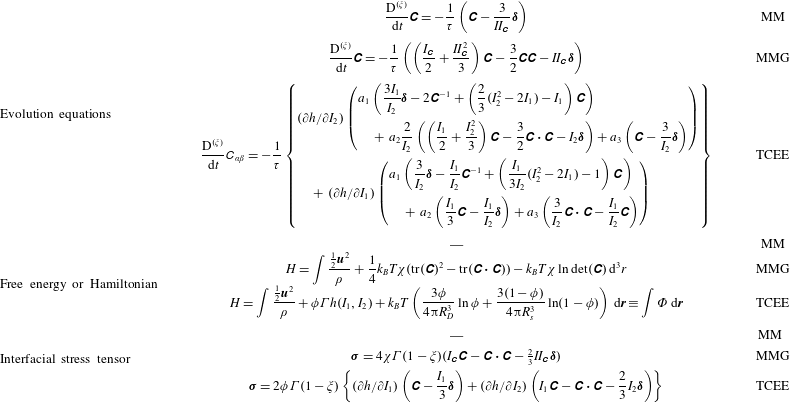
3.6 Asymptotic behaviour of the conformation tensor model
The results of a perturbation expansion are now presented to demonstrate that the TCEE model equations are in fact consistent with the microscopic theory presented in (2.13). The derivation of the perturbation expansion of the conformation tensor
 $\unicode[STIX]{x1D60A}_{\unicode[STIX]{x1D6FC}\unicode[STIX]{x1D6FD}}$
in the small parameter, the characteristic time
 $\unicode[STIX]{x1D70F}_{C}=\unicode[STIX]{x1D707}R/\unicode[STIX]{x1D6FE}$
, leads to
 $$\begin{eqnarray}\unicode[STIX]{x1D60A}_{\unicode[STIX]{x1D6FC}\unicode[STIX]{x1D6FD}}=\unicode[STIX]{x1D60A}_{0,\unicode[STIX]{x1D6FC}\unicode[STIX]{x1D6FD}}+\unicode[STIX]{x1D70F}_{C}\unicode[STIX]{x1D60A}_{1,\unicode[STIX]{x1D6FC}\unicode[STIX]{x1D6FD}}+\frac{\unicode[STIX]{x1D70F}_{C}^{2}}{2}\unicode[STIX]{x1D60A}_{2,\unicode[STIX]{x1D6FC}\unicode[STIX]{x1D6FD}}+O(\unicode[STIX]{x1D70F}^{3}),\end{eqnarray}$$
where
 $$\begin{eqnarray}\displaystyle & \displaystyle \unicode[STIX]{x1D60A}_{\unicode[STIX]{x1D6FC}\unicode[STIX]{x1D6FD}}=\unicode[STIX]{x1D6FF}_{\unicode[STIX]{x1D6FC}\unicode[STIX]{x1D6FD}}, & \displaystyle\end{eqnarray}$$
 $$\begin{eqnarray}\displaystyle & \displaystyle \unicode[STIX]{x1D60A}_{1,\unicode[STIX]{x1D6FC}\unicode[STIX]{x1D6FD}}=\frac{2(1-\unicode[STIX]{x1D709})D_{\unicode[STIX]{x1D6FC}\unicode[STIX]{x1D6FD}}}{(a_{1}+a_{2}+a_{3})(A_{1}+A_{2})}, & \displaystyle\end{eqnarray}$$
with
 $$\begin{eqnarray}A_{1}\equiv \unicode[STIX]{x2202}h/\unicode[STIX]{x2202}I_{1}|_{\unicode[STIX]{x1D70F}_{C}=0}=\frac{\unicode[STIX]{x1D714}}{48}(2-\unicode[STIX]{x1D714})\quad \text{and}\quad A_{2}\equiv \unicode[STIX]{x2202}h/\unicode[STIX]{x2202}I_{2}|_{\unicode[STIX]{x1D70F}_{C}=0}=\frac{\unicode[STIX]{x1D714}}{48}(2+\unicode[STIX]{x1D714})\end{eqnarray}$$
and
 $$\begin{eqnarray}\displaystyle & & \displaystyle \unicode[STIX]{x1D60A}_{2,\unicode[STIX]{x1D6FC}\unicode[STIX]{x1D6FD}}=\frac{2(1-\unicode[STIX]{x1D709})}{(a_{1}+a_{2}+a_{3})^{2}(A_{1}+A_{2})^{2}}\nonumber\\ \displaystyle & & \displaystyle \times \left(\begin{array}{@{}l@{}}\displaystyle -2\left(\frac{\text{DD}_{\unicode[STIX]{x1D6FC}\unicode[STIX]{x1D6FD}}}{\text{d}t}-(\unicode[STIX]{x1D6FA}_{\unicode[STIX]{x1D6FC}\unicode[STIX]{x1D6FE}}\unicode[STIX]{x1D60B}_{\unicode[STIX]{x1D6FE}\unicode[STIX]{x1D6FD}}-D_{\unicode[STIX]{x1D6FC}\unicode[STIX]{x1D6FE}}\unicode[STIX]{x1D6FA}_{\unicode[STIX]{x1D6FE}\unicode[STIX]{x1D6FD}})\right)\\ \displaystyle \quad +\,\frac{2(1-\unicode[STIX]{x1D709})}{(a_{1}+a_{2}+a_{3})(A_{1}+A_{2})}\left(\begin{array}{@{}l@{}}\displaystyle (A_{2}(6a_{1}+4a_{2}+2a_{3})+A_{1}(4a_{1}+2a_{2}))D_{\unicode[STIX]{x1D6FC}\unicode[STIX]{x1D6FE}}\unicode[STIX]{x1D60B}_{\unicode[STIX]{x1D6FE}\unicode[STIX]{x1D6FD}}\\ \displaystyle \quad -\,\frac{\text{tr}(\unicode[STIX]{x1D63F}\unicode[STIX]{x1D63F})}{3}(A_{2}(5a_{1}+3a_{2}+a_{3})+A_{1}(3a_{1}+a_{2}-a_{3}))\unicode[STIX]{x1D6FF}_{\unicode[STIX]{x1D6FC}\unicode[STIX]{x1D6FD}}\end{array}\right)\end{array}\right).\nonumber\\ \displaystyle & & \displaystyle\end{eqnarray}$$
Subsequently, substitution of this result into the stress tensor in (3.31) results in
 $$\begin{eqnarray}\displaystyle \unicode[STIX]{x1D748} & = & \displaystyle 2\unicode[STIX]{x1D707}\unicode[STIX]{x1D63F}+\unicode[STIX]{x1D719}\unicode[STIX]{x1D707}P(\unicode[STIX]{x1D706})2\unicode[STIX]{x1D63F}+\left(\frac{2\unicode[STIX]{x1D719}\unicode[STIX]{x1D6E4}\unicode[STIX]{x1D70F}_{C}(1-\unicode[STIX]{x1D709})^{2}}{(a_{1}+a_{2}+a_{3})}\right)\nonumber\\ \displaystyle & & \displaystyle \times \,\left(2\unicode[STIX]{x1D63F}-\frac{\unicode[STIX]{x1D70F}_{C}}{(a_{1}+a_{2}+a_{3})(A_{1}+A_{2})}\left\{\begin{array}{@{}l@{}}\displaystyle 2\left(\frac{\text{D}}{\text{D}t}\unicode[STIX]{x1D63F}-(\unicode[STIX]{x1D734}\boldsymbol{\cdot }\unicode[STIX]{x1D63F}-\unicode[STIX]{x1D63F}\boldsymbol{\cdot }\unicode[STIX]{x1D734})\right)\\ \displaystyle \quad -\,\frac{4(1-\unicode[STIX]{x1D709})(2a_{1}+a_{2})}{(a_{1}+a_{2}+a_{3})}\left(\unicode[STIX]{x1D63F}\boldsymbol{\cdot }\unicode[STIX]{x1D63F}-\frac{\text{tr}(\unicode[STIX]{x1D63F}\boldsymbol{\cdot }\unicode[STIX]{x1D63F})}{3}\unicode[STIX]{x1D644}\right)\end{array}\right\}\right)\nonumber\\ \displaystyle & & \displaystyle +\,O(\unicode[STIX]{x1D70F}_{C}^{3}).\end{eqnarray}$$
For comparison with (3.39), (2.13) is rewritten in an analogous form given by
 $$\begin{eqnarray}\displaystyle \unicode[STIX]{x1D748} & = & \displaystyle 2\unicode[STIX]{x1D707}\unicode[STIX]{x1D63F}+\unicode[STIX]{x1D719}\left(\frac{5\unicode[STIX]{x1D706}+2}{2(\unicode[STIX]{x1D706}+1)}\right)\unicode[STIX]{x1D707}\nonumber\\ \displaystyle & & \displaystyle \times \,\!\!\left(2\unicode[STIX]{x1D63F}-\unicode[STIX]{x1D713}_{1}\!\left\{2\!\left(\frac{\text{D}}{\text{D}t}\unicode[STIX]{x1D63F}-(\unicode[STIX]{x1D734}\boldsymbol{\cdot }\unicode[STIX]{x1D63F}-\unicode[STIX]{x1D63F}\boldsymbol{\cdot }\unicode[STIX]{x1D734})\right)\!-\unicode[STIX]{x1D713}_{2}\!\left(\unicode[STIX]{x1D63F}\boldsymbol{\cdot }\unicode[STIX]{x1D63F}-\frac{\text{tr}(\unicode[STIX]{x1D63F}\boldsymbol{\cdot }\unicode[STIX]{x1D63F})}{3}\unicode[STIX]{x1D644}\right)\!\right\}\!\right)\!+\!O(Ca^{2}),\nonumber\\ \displaystyle & & \displaystyle\end{eqnarray}$$
where we also include a purely viscous term to account for the dissipation due to a solvent of viscosity
 $\unicode[STIX]{x1D707}$
. In this expression, the second-order coefficients are (Schowalter et al.
Reference Schowalter, Chaffey and Brenner1968)
 $$\begin{eqnarray}\unicode[STIX]{x1D713}_{1}=\left[\frac{Ca^{\ast }}{40}\left(\frac{(19\unicode[STIX]{x1D706}+16)^{2}}{(\unicode[STIX]{x1D706}+1)(5\unicode[STIX]{x1D706}+2)}\right)\right]\end{eqnarray}$$
and
 $$\begin{eqnarray}\unicode[STIX]{x1D713}_{2}=\frac{12(25\unicode[STIX]{x1D706}^{2}+41\unicode[STIX]{x1D706}+4)}{7(19\unicode[STIX]{x1D706}+16)(\unicode[STIX]{x1D706}+1)},\end{eqnarray}$$
where
 $Ca^{\ast }=\unicode[STIX]{x1D707}R/\unicode[STIX]{x1D6FE}=\unicode[STIX]{x1D70F}_{C}$
.
It is important to realize that on comparing (3.39) and (3.40), they have the same form and all process-dependent terms are common. This shows the consistency of the NET approach. In fact, full consistency can be achieved if the following constraint equations are satisfied:
 $$\begin{eqnarray}\displaystyle & \displaystyle \frac{2\unicode[STIX]{x1D6E4}\unicode[STIX]{x1D70F}_{C}^{2}(1-\unicode[STIX]{x1D709})^{2}}{(a_{1}+a_{2}+a_{3})^{2}(A_{1}+A_{2})}=\unicode[STIX]{x1D713}_{1}\left(\frac{5\unicode[STIX]{x1D706}+2}{2(\unicode[STIX]{x1D706}+1)}\right)\unicode[STIX]{x1D707}, & \displaystyle\end{eqnarray}$$
 $$\begin{eqnarray}\displaystyle & \displaystyle \frac{4(1-\unicode[STIX]{x1D709})(2a_{1}+a_{2})}{(a_{1}+a_{2}+a_{3})}=\unicode[STIX]{x1D713}_{2} & \displaystyle\end{eqnarray}$$
and
 $$\begin{eqnarray}\unicode[STIX]{x1D707}P(\unicode[STIX]{x1D706})+\frac{2\unicode[STIX]{x1D6E4}\unicode[STIX]{x1D70F}_{C}(1-\unicode[STIX]{x1D709})^{2}}{(a_{1}+a_{2}+a_{3})}=\left(\frac{5\unicode[STIX]{x1D706}+2}{2(\unicode[STIX]{x1D706}+1)}\right)\unicode[STIX]{x1D707}.\end{eqnarray}$$
In the section that follows, we use these expressions and other additional information, all available a priori, to fully define all parameters of the TCEE model, at least in the limit of slow, slowly varying flows.
3.7 Determining model parameters from asymptotic solutions
In total, the model has five macroscopic parameters,
 $\unicode[STIX]{x1D709}$
,
 $P(\unicode[STIX]{x1D706})$
,
 $a_{1}$
,
 $a_{2}$
and
 $a_{3}$
. In general, there are many combinations of these parameters that may be used to develop a model that is consistent with the
 $O(Ca^{2})$
expansion characterized by (3.43)–(3.45), albeit involving some parameters as degrees of freedom that can be expanded even further if more involved expressions are used for the dissipation. Additional microscopic information on the morphology of the ellipsoid droplet, beyond agreement with the stress tensor to
 $O(Ca^{2})$
, is required to remove any ambiguity. To enforce such agreement with microscopic theory (Frankel & Acrivos Reference Frankel and Acrivos1970; Barthes-Bièsel & Acrivos Reference Barthes-Bièsel and Acrivos1973; Rallison Reference Rallison1980), we first write the dimensionless form of (3.3) as
 $$\begin{eqnarray}r^{2}\unicode[STIX]{x1D60A}_{ij}^{-1}n_{i}n_{j}=1,\end{eqnarray}$$
where
 $n_{i}\equiv r_{i}/r$
and
 $r\equiv (r_{i}r_{i})^{1/2}$
is the distance from the centre of the ellipse to a position on its surface characterized by
 $\boldsymbol{r}$
such that
 $(n_{i}n_{i})^{1/2}\equiv 1$
. We note that
 $r^{2}$
and
 $\unicode[STIX]{x1D60A}_{ij}$
carry related information, but at different levels of description; the former is primarily used in microscopic theory while the latter is employed in macroscopic conformation-tensor-based models. Therefore, this relationship is important in enforcing consistency between microscopic and macroscopic descriptions of ellipsoidal morphology. It also allows us to determine additional constraints on the parameters in the model. By comparing the evolution of the first-order perturbation to an equilibrium droplet, i.e. the evolution of
 $\unicode[STIX]{x1D60A}_{1,\unicode[STIX]{x1D6FC}\unicode[STIX]{x1D6FD}}$
in (3.34), with the corresponding microscopic analysis of droplet deformation by Barthes-Bièsel & Acrivos (Reference Barthes-Bièsel and Acrivos1973) to
 $O(1)$
(Rallison 1981), we find that (see appendix D)
 $$\begin{eqnarray}(1-\unicode[STIX]{x1D709})=\frac{5}{(2\unicode[STIX]{x1D706}+3)}\equiv f_{1}\end{eqnarray}$$
and
 $$\begin{eqnarray}(a_{1}+a_{2}+a_{3})(A_{1}+A_{2})=\frac{40(\unicode[STIX]{x1D706}+1)}{(19\unicode[STIX]{x1D706}+16)(2\unicode[STIX]{x1D706}+3)}\equiv f_{2}.\end{eqnarray}$$
These definitions ensure that the conformation tensor model is at least consistent with the
 $O(1)$
Taylor deformation theory at infinitesimal capillary numbers. An immediate consequence of (3.47) and (3.48) is that, asymptotically, the selection of
 $\unicode[STIX]{x1D714}=8/5$
results in (3.43) being identically satisfied. This is very important as it provides an independent validation of the self-consistency of the proposed approach and a justification for the use of the more correct value of
 $\unicode[STIX]{x1D714}=8/5$
in (3.27) for small deviations from sphericity (see appendix B). Thus, we are left with only four independent equations, (3.44), (3.45), (3.47) and (3.48), to determine the model parameters.
To avoid the need for any adjustment right now, we decide to use the lower-order weight
 $a_{1}=0$
. This allows us to develop a relaxation model with terms reminiscent of the MM and MMG models. The remaining four model parameters,
 $\unicode[STIX]{x1D709}$
,
 $P(\unicode[STIX]{x1D706})$
,
 $a_{2}$
and
 $a_{3}$
, can then be fully determined from (3.44), (3.45), (3.47) and (3.48) as
 $$\begin{eqnarray}\displaystyle & \displaystyle a_{1}=0, & \displaystyle\end{eqnarray}$$
 $$\begin{eqnarray}\displaystyle & \displaystyle a_{2}=\frac{\unicode[STIX]{x1D713}_{2}f_{2}}{4f_{1}(A_{1}+A_{2})}, & \displaystyle\end{eqnarray}$$
 $$\begin{eqnarray}\displaystyle & \displaystyle a_{3}=\frac{f_{2}}{(A_{1}+A_{2})}-\frac{\unicode[STIX]{x1D713}_{2}f_{2}}{4f_{1}(A_{1}+A_{2})}, & \displaystyle\end{eqnarray}$$
 $$\begin{eqnarray}\displaystyle & \displaystyle \unicode[STIX]{x1D709}=1-\frac{5}{(2\unicode[STIX]{x1D706}+3)} & \displaystyle\end{eqnarray}$$
and
 $$\begin{eqnarray}P(\unicode[STIX]{x1D706})=\frac{(5\unicode[STIX]{x1D706}+2)}{2(\unicode[STIX]{x1D706}+1)}\left(1-\frac{(19\unicode[STIX]{x1D706}+16)}{(5\unicode[STIX]{x1D706}+2)(2\unicode[STIX]{x1D706}+3)}\right).\end{eqnarray}$$
It should be noted that all parameters depend on the viscosity ratio
 $\unicode[STIX]{x1D706}$
, reflecting their dissipative nature. In the following, we present the results of the asymptotic model developed here and compare them with experimental data.
4 Application of the TCEE model to small-
$Ca$
flows

In this section, the predictions of the TCEE model employing the parameters described in § 3.7, as given by (3.28), (3.29), (3.31), (3.33) and (3.49)–(3.53), are presented for a class of simple flows with prescribed kinematics for which other numerical and/or experimental results are available at small but finite
 $Ca$
to further evaluate the model.
4.1 Steady shear flows
In figures 2 and 3, we compare the TCEE model predictions for the principal stress components with numerical results from Kennedy, Pozrikidis & Skalak (Reference Kennedy, Pozrikidis and Skalak1994) and the corresponding theoretical predictions of Schowalter et al. (Reference Schowalter, Chaffey and Brenner1968) in (2.13) for small-
 $Ca$
steady simple shear flows, for
 $\unicode[STIX]{x1D706}=1$
and
 $\unicode[STIX]{x1D706}=6.4$
respectively. Also presented for
 $\unicode[STIX]{x1D706}=1$
in figure 2 are results obtained from the droplet conformation predictions of the MM model through the use of the stress expression obtained by Batchelor (Reference Batchelor1970) as given by (1.6) in Doi & Ohta (Reference Doi and Ohta1991). Similar stress predictions for
 $\unicode[STIX]{x1D706}=6.4$
using this approach require information on the interface velocity and cannot be obtained without resorting to microscopic calculations. Therefore, the key advantage of the TCEE model (and thermodynamically consistent models in general) over phenomenological, solely structural, models like the MM model is that an accurate expression for the stress tensor can always be obtained directly through expressions like (3.31).
However, it is of interest to note that, as seen in figure 2 for
 $\unicode[STIX]{x1D706}=1$
, the predictions from the TCEE and MM models are very close, almost indistinguishable, especially at lower
 $Ca$
. In retrospect, this is what one should have expected as both models are built up based on fitting asymptotic results, the MM model just for the conformation (because only this is involved there) and the TCEE model for both the conformation and the stress. The fact that Batchelor’s expression for stress comes so close to the TCEE model stress predictions provides additional evidence of the internal consistency of our approach, which is fundamentally based on a connection between the stress and the structure. The only difference is that in order to fully enforce this connection in our approach, one requires independent results for the stress to fit the scalar parameters involved in the model. In exchange, what one gets with this approach of indirectly enforcing the connection between the stress and the structure, as opposed to using a direct relationship such as that of Batchelor (Reference Batchelor1970), is an easier evaluation and a more general one valid for all
 $\unicode[STIX]{x1D706}$
values, instead of just
 $\unicode[STIX]{x1D706}=1$
. In both figures 2 and 3, the TCEE model captures well the trends in the numerical results, especially at the small
 $Ca$
values for which the model parameters have been developed. Furthermore, the predictions of the rheology at larger capillary numbers are reasonable and demonstrate the robustness of the TCEE model.
Model predictions of the stress tensor components as a function of the capillary number
 $(Ca)$
compared with simulation results (symbols) from Kennedy et al. (Reference Kennedy, Pozrikidis and Skalak1994) for
 $\unicode[STIX]{x1D706}=1$
. The solid lines are TCEE model predictions using (3.31), the dotted lines are predictions from the MM model using the stress expression of Batchelor (Reference Batchelor1970) and the dashed lines are predictions from the asymptotic theory in (2.13). In applying (2.13) and (3.31), the dissipation of the medium is neglected and the stress tensor is scaled by the interfacial energy density
 $\unicode[STIX]{x1D6FE}/R$
such that
 $\unicode[STIX]{x1D70E}_{\unicode[STIX]{x1D6FC}\unicode[STIX]{x1D6FD}}^{\ast }=\unicode[STIX]{x1D70E}_{\unicode[STIX]{x1D6FC}\unicode[STIX]{x1D6FD}}R/\unicode[STIX]{x1D6FE}$
.

Model predictions of the stress tensor components as a function of the capillary number
 $(Ca)$
compared with simulation results (symbols) from Kennedy et al. (Reference Kennedy, Pozrikidis and Skalak1994) for
 $\unicode[STIX]{x1D706}=6.4$
. The solid lines are TCEE model predictions using (3.31) while the dashed lines are predictions from the asymptotic theory in (2.13). In applying (2.13) and (3.31), the dissipation of the medium is neglected and the stress tensor is scaled by the interfacial energy density
 $\unicode[STIX]{x1D6FE}/R$
such that
 $\unicode[STIX]{x1D70E}_{\unicode[STIX]{x1D6FC}\unicode[STIX]{x1D6FD}}^{\ast }=\unicode[STIX]{x1D70E}_{\unicode[STIX]{x1D6FC}\unicode[STIX]{x1D6FD}}R/\unicode[STIX]{x1D6FE}$
.

Model predictions of the droplet deformation
 $D_{T}$
(a,b) and orientation angle (c,d) as a function of the capillary number
 $(Ca)$
compared with simulation results (symbols) from Kennedy et al. (Reference Kennedy, Pozrikidis and Skalak1994) for
 $\unicode[STIX]{x1D706}=1$
(a,c) and
 $\unicode[STIX]{x1D706}=6.4$
(b,d). Also shown with dot-dashed lines in (a,b) are theoretical results by Taylor (Reference Taylor1934) for the deformation parameter using (4.2) and in (c,d) theoretical results by Chaffey & Brenner (Reference Chaffey and Brenner1967) using (4.3) for the orientation angle. The solid lines are TCEE model predictions and the dashed lines are MM model predictions.

In figure 4(a,b), we present the TCEE model predictions of the Taylor deformation parameter, defined as
 $$\begin{eqnarray}D_{T}=\frac{(L-B)}{(L+B)},\end{eqnarray}$$
where
 $L$
and
 $B$
are the semi-axes of the emulsion droplet projected in the flow–gradient plane, for
 $\unicode[STIX]{x1D706}=1$
and
 $\unicode[STIX]{x1D706}=6.4$
respectively. It should be noted that as far as the TCEE model is concerned, its predictions for steady simple shear flow involve a structure with mirror symmetry with respect to the flow–gradient plane. Thus, in this case,
 $L$
and
 $B$
are the major and minor axis of the ellipsoid, as shown in figure 1. In figure 4(c,d), we present the TCEE model predictions for the droplet orientation angle
 $\unicode[STIX]{x1D703}$
relative to the flow direction for the same values of
 $\unicode[STIX]{x1D706}$
. Also included in the same figure for comparison purposes are the simulation results of Kennedy et al. (Reference Kennedy, Pozrikidis and Skalak1994), the MM model predictions and theoretical calculations, to first order, of the Taylor deformation parameter, given as (Taylor Reference Taylor1934)
 $$\begin{eqnarray}D_{T}=\frac{19\unicode[STIX]{x1D706}+16}{16\unicode[STIX]{x1D706}+16}Ca,\end{eqnarray}$$
and of the orientation angle in simple shear flow, given as (Chaffey & Brenner Reference Chaffey and Brenner1967)
 $$\begin{eqnarray}\unicode[STIX]{x1D703}=\frac{\unicode[STIX]{x03C0}}{4}-\frac{(2\unicode[STIX]{x1D706}+3)(19\unicode[STIX]{x1D706}+16)}{80(\unicode[STIX]{x1D706}+1)}Ca.\end{eqnarray}$$
The TCEE model and MM model provide similar predictions of the trends observed in the experimental data at small capillary numbers. However, at larger capillary numbers, the nonlinear effects entering the two models are distinct, and the predictions from the two models are slightly different. This is not surprising because although the relaxation terms in the two models differ, the parameters entering the conformation tensor equation in both models are selected to be consistent with the results of Barthes-Bièsel & Acrivos (Reference Barthes-Bièsel and Acrivos1973) to
 $O(1)$
in
 $Ca$
only. Therefore, the distinct advantage of the TCEE model is that in addition to providing equally good approximations of the droplet deformation and orientation to those in the previous MM model, it also provides good predictions of the stress tensor at all viscosity ratios, as shown in figures 2 and 3.
As seen in figure 4(a,c), for
 $\unicode[STIX]{x1D706}=1$
, the TCEE model predictions of the droplet deformation and orientation are in good agreement with the experimental data. However, as seen in figure 4(b,d), for
 $\unicode[STIX]{x1D706}=6.4$
, the TCEE model shows larger deviations from the experimental data, albeit, in this case, the agreement is much better than that of the asymptotic results which clearly miss the observed trends. The much better agreement seen in the corresponding stress predictions from the TCEE model in figure 3 for
 $\unicode[STIX]{x1D706}=6.4$
may be partly attributed to the fact that the TCEE model stress predictions are forced to be consistent with the stress tensor results of Schowalter et al. (Reference Schowalter, Chaffey and Brenner1968) to
 $O(Ca^{2})$
. On the other hand, the conformation tensor results are only enforced to be
 $O(1)$
accurate with respect to the results of Barthes-Bièsel & Acrivos (Reference Barthes-Bièsel and Acrivos1973). This may partly explain the relatively weaker agreement seen in figure 4(b,d) for
 $\unicode[STIX]{x1D706}=6.4$
between the TCEE model and the simulation results for the droplet deformation and orientation compared with that seen in figure 4(a,c) for
 $\unicode[STIX]{x1D706}=1$
. More specifically, as the viscosity ratio increases, nonlinear effects on the droplet deformation (which require a complex description of the non-affine motion) may be more important. Still, the improvement over the asymptotic results from which the TCEE model emerges is impressive.
As previously noted, the agreement between the TCEE model and the simulation data may be improved by introducing additional corrective terms. For example, such corrective effects may be introduced into the model through more complex dissipative terms in the TCEE model which are selected to be consistent with the results of Barthes-Bièsel & Acrivos (Reference Barthes-Bièsel and Acrivos1973) to higher order. On the other hand, although better predictions for simple shear flow can also be achieved by allowing for a nonlinear dependence of
 $\unicode[STIX]{x1D709}$
on the capillary number, this is a change that destroys the thermodynamic consistency of the model. This can result in aphysical predictions in more general flows. Ultimately, this brings out the important point that the conformation tensor equation and the expression for the stress tensor are not independent in the context of a thermodynamically consistent model. Therefore, care must be exercised when modifying model parameters. As a result, we do not attempt any phenomenological modification to
 $\unicode[STIX]{x1D709}$
based on the capillary number. Modifications based on the conformation tensor through the invariants as well as additional nonlinearity in the dissipation are allowed, but we delegate such improvements to a future publication in order to keep the analysis here as simple as possible. On the other hand, for
 $\unicode[STIX]{x1D706}=1$
, non-affine effects are less important and the
 $O(1)$
approximation of the results of Barthes-Bièsel & Acrivos (Reference Barthes-Bièsel and Acrivos1973) used to develop some of the TCEE model parameters is more accurate. Consequently, the TCEE model predictions for the droplet deformation, orientation and stress tensor in figures 4(a), 4(c) and 2 respectively provide a good representation of the numerical results in this case.
Model predictions of the droplet deformation
 $D_{T}$
(a,b) and orientation angle
 $\unicode[STIX]{x1D703}$
(c,d) as a function of the capillary number
 $(Ca)$
compared with experimental results (symbols) from Torza et al. (Reference Torza, Cox and Mason1972) for
 $\unicode[STIX]{x1D706}=0.08$
(a,c) and
 $\unicode[STIX]{x1D706}=3.6$
(b,d). Also shown with dot-dashed lines in (a,b) are theoretical results by Taylor (Reference Taylor1934) for the deformation parameter using (4.2) and in (c,d) theoretical results by Chaffey & Brenner (Reference Chaffey and Brenner1967) using (4.3) for the orientation angle. The solid lines are TCEE model predictions and the dashed lines are MM model predictions.

Next, the TCEE model predictions are compared with experimental data for the droplet deformation and orientation from Torza et al. (Reference Torza, Cox and Mason1972) in a dilute emulsion of oxidized castor oil in two different silicone oils corresponding to
 $\unicode[STIX]{x1D706}=0.08$
and
 $\unicode[STIX]{x1D706}=3.6$
. In figure 5, we compare the TCEE model predictions for droplet deformation and orientation with the experimental data as well as the predictions of the MM model. It should be noted again that both the TCEE and the MM models provide similar predictions of the trends observed in the experimental data for similar reasons discussed before in relation to the predictions shown in figure 4. Moreover, in figure 5, similarly to the comparison with the numerical results of Kennedy et al. (Reference Kennedy, Pozrikidis and Skalak1994) in figure 4, the comparison of the model predictions of the Taylor deformation parameter with the experimental data of Torza et al. (Reference Torza, Cox and Mason1972) for high viscosity ratios becomes poor as the capillary number increases. Similarly to the comments in the previous paragraph, the agreement can be improved by using the nonlinear extension of
 $\unicode[STIX]{x1D709}$
by allowing a direct dependence on the capillary number as in the MM model (Maffettone & Minale Reference Maffettone and Minale1998). However, as mentioned before, this comes at the risk of aphysical behaviour in more general flows. An additional remark that can be made based on both figures 4 and 5 is that the TCEE model predictions (and those of the original MM model) work best for
 $\unicode[STIX]{x1D706}\leqslant 1$
. The less satisfactory agreement with experimental and numerical data at higher viscosity ratios may be attributed to the increasing importance of non-affine effects as the droplets effectively become more rigid. As a concluding remark, there is a clear need to work on better non-affine representations, but only if they are compatible with the bracket scheme followed in this work in order to avoid aphysical results.
Finally, for completeness, in table 2, the numerical values of the parameters corresponding to the predictions of the TCEE model in figure 5 are summarized. The presence of a negative value for
 $a_{3}$
may raise concerns regarding the thermodynamic admissibility of this parameter value. This is examined by investigating whether the thermodynamic consistency criterion requiring a positive relaxation dissipation density, given by
 $$\begin{eqnarray}\unicode[STIX]{x1D6F7}=\unicode[STIX]{x1D6EC}_{\unicode[STIX]{x1D6FC}\unicode[STIX]{x1D6FD}\unicode[STIX]{x1D6FE}\unicode[STIX]{x1D700}}\left(\frac{\unicode[STIX]{x1D6FF}H}{\unicode[STIX]{x1D6FF}\unicode[STIX]{x1D60A}_{\unicode[STIX]{x1D6FE}\unicode[STIX]{x1D700}}}-\frac{1}{3}\unicode[STIX]{x1D60A}_{\unicode[STIX]{x1D70C}\unicode[STIX]{x1D702}}\frac{\unicode[STIX]{x1D6FF}H}{\unicode[STIX]{x1D6FF}\unicode[STIX]{x1D60A}_{\unicode[STIX]{x1D70C}\unicode[STIX]{x1D702}}}\unicode[STIX]{x1D60A}_{\unicode[STIX]{x1D6FE}\unicode[STIX]{x1D700}}^{-1}\right)\left(\frac{\unicode[STIX]{x1D6FF}H}{\unicode[STIX]{x1D6FF}\unicode[STIX]{x1D60A}_{\unicode[STIX]{x1D6FC}\unicode[STIX]{x1D6FD}}}-\frac{1}{3}\unicode[STIX]{x1D60A}_{\unicode[STIX]{x1D70C}\unicode[STIX]{x1D702}}\frac{\unicode[STIX]{x1D6FF}H}{\unicode[STIX]{x1D6FF}\unicode[STIX]{x1D60A}_{\unicode[STIX]{x1D70C}\unicode[STIX]{x1D702}}}\unicode[STIX]{x1D60A}_{\unicode[STIX]{x1D6FC}\unicode[STIX]{x1D6FD}}^{-1}\right)\geqslant 0,\end{eqnarray}$$
is satisfied in this case. This measure has been computed numerically, as a function of the capillary number, and is found to be always positive. Moreover, a negative value of
 $P(\unicode[STIX]{x1D706})$
such as that seen in the first column of table 2 is admissible as long as the overall effective viscosity remains positive, which can certainly be enforced in the case of the dilute limit
 $\unicode[STIX]{x1D719}\rightarrow 0$
, as the contribution of the
 $P(\unicode[STIX]{x1D706})$
term in the viscosity is weighted by
 $\unicode[STIX]{x1D719}$
(see (3.31)).
Summary of model parameters corresponding to the microstructure predictions of the TCEE model in figure 5.
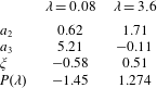
4.2 Transient simple shear flow
So far, the numerical and experimental data sets used to validate the TCEE model have been steady-state shear flow results. In this subsection, the TCEE model is compared with time-dependent shear flow experiments (Guido & Villone Reference Guido and Villone1998) obtained using a dilute emulsion system of polyisobutylene (PIB) and polydimethylsiloxane (PDMS) with
 $\unicode[STIX]{x1D706}=1.4$
. In figure 6, we examine the evolution of the three dimensionless droplet semi-axes as a function of strain in the start-up of shear flow for
 $Ca=0.24$
and
 $\unicode[STIX]{x1D706}=1.4$
. It should be noted that the TCEE model predictions agree very well with the experimental data and describe the principal axes of the deforming droplet better than the MM model. Experimental results such as those in figure 6 are important in distinguishing the predictive capability of the two models as it is well known that the Taylor deformation parameter
 $D_{T}$
, defined in (4.1), is not a rigorous measure of the droplet deformation. Therefore, unlike the experimental results for droplet deformation in figures 4 and 5, which are inconclusive, the comparison in figure 6 shows that the TCEE model provides significantly better predictions of the dimensionless semi-axes of the deforming droplet than the MM model.
Model predictions for the three non-dimensional axes of the droplet as a function of applied strain for transient start-up shear flow corresponding to
 $Ca=0.24$
and
 $\unicode[STIX]{x1D706}=1.4$
compared with experimental data. The open and filled symbols correspond to experiments at two different digitization settings (Guido & Villone Reference Guido and Villone1998). The solid lines correspond to the predictions of the TCEE model and the dashed lines correspond to the predictions of the MM model.

4.3 Steady-state flow in a four-roll mill
Here, we compare the TCEE model predictions for the deformation and orientation of a droplet with experimental results of Bentley & Leal (Reference Bentley and Leal1986) obtained through the use of a four-roll mill device. In these experiments, the velocity gradient tensor around the droplet is steady and is defined as
 $$\begin{eqnarray}\unicode[STIX]{x1D735}\unicode[STIX]{x1D66B}=\frac{1}{2}\dot{\unicode[STIX]{x1D6FE}}\left[\begin{array}{@{}ccc@{}}1+\unicode[STIX]{x1D6FC} & 1-\unicode[STIX]{x1D6FC} & 0\\ -1+\unicode[STIX]{x1D6FC} & -1-\unicode[STIX]{x1D6FC} & 0\\ 0 & 0 & 0\end{array}\right],\end{eqnarray}$$
where the dimensionless parameter
 $0\leqslant \unicode[STIX]{x1D6FC}\leqslant 1$
specifies the relative strength of the strain rate and vorticity in the flow. The limit of
 $\unicode[STIX]{x1D6FC}=1$
represents purely straining flow while
 $\unicode[STIX]{x1D6FC}=0$
represents simple shear flow. In figure 7, we compare the TCEE model predictions with the experimental results of Bentley & Leal (Reference Bentley and Leal1986) as well as the predictions of the MM model for the deformation (figure 7
a) and orientation (figure 7
b) of a droplet in the flow field defined in (4.5). As shown there, the TCEE model captures well the deformation observed at low capillary numbers, but its predictions deviate from experimental data as the capillary number increases. The deviation of the model from the experimental data occurs when an upturn is observed in the experimentally measured deformation parameter prior to breakup. Under these circumstances, the actual droplet shape is expected to begin to deviate significantly from an ellipsoidal shape, which violates a critical assumption of the TCEE model. Therefore, at larger
 $Ca$
, the TCEE model is not expected to describe the real system. Still, the success of the model at small capillary numbers indicates the utility of employing asymptotic theory in constraining the small-capillary-number response of the TCEE model. It should be noted that for those small
 $Ca$
values, the predictions of the TCEE and MM models are practically indistinguishable.
Model predictions of (a) the droplet deformation,
 $D_{T}$
, and (b) the orientation angle,
 $\unicode[STIX]{x1D703}$
, as a function of
 $Ca$
for
 $\unicode[STIX]{x1D706}=6.5$
compared with experimental data. The experimental data (symbols) are from Bentley & Leal (Reference Bentley and Leal1986). Arrows indicate an increasing value of the flow parameter
 $\unicode[STIX]{x1D6FC}$
defined by (4.5) assuming the values 0.2, 0.4, 0.6, 0.8 and 1. The solid lines correspond to the predictions of the TCEE model and the dashed lines correspond to the predictions of the MM model.

5 Conclusions
In this work, we developed an internal conformation-tensor-based macroscopic rheological model for dilute emulsions through a rigorous and systematic bracket theory. We started by first probing the consequences of the microscopic physical interpretation of the conformation tensor that was chosen to describe approximately the deformed droplet geometry as an ellipsoid. This microscopic interpretation was first used to independently construct an extended free energy expression for a dilute emulsion. This expression takes into account the surface-free energy of the deformed droplets and can conveniently be evaluated in a closed form based on a powerful approximation for the surface of an ellipsoid in terms of the first and second invariants of the conformation tensor. Following the definition of the conformation tensor for infinitesimal deformations under conditions for which there is purely affine motion, we then demonstrated its contravariant tensorial character since, under those conditions, it coincides with the (contravariant) Cauchy strain tensor. The appropriate Poisson bracket was then developed by suitably modifying the standard Poisson bracket for contravariant tensors, taking into account the unit determinant constraint imposed due to the droplet volume conservation. That constraint modifies the dissipation bracket as well, from which a general low-order (in Volterra derivatives with respect to the conformation tensor) expression was developed in terms of a minimum of four dissipation parameters. The final model that resulted as a consequence of the application of the Poisson and dissipation bracket dynamics was then shown to be capable of providing asymptotic predictions for the flow-induced structures and extra stress that are fully consistent with available asymptotic theories for both the internal droplet structure and the macroscopic extra stress tensor. We took advantage of this result to use these asymptotic theories to fully determine all four dissipation model parameters. Then, we validated the model through comparisons with experimental and simulation data for small capillary numbers in various flows with prespecified kinematics ranging from steady and transient simple shear to a linear combination of simple shear and pure straining flow. In all cases, the TCEE model produces results that are physical and reliably extend the asymptotic results valid at infinitesimally small capillary number to small but finite values.
Comparison of the TCEE model evolution equation with the MM model of Maffettone & Minale (Reference Maffettone and Minale1998) and the MMG model of Grmela et al. (Reference Grmela, Ammar, Chinesta and Maîtrejean2014) reveals these as particular subcases corresponding to particular approximations for the free energy and particular selections of the relaxation dissipation. Still, we need to note here that the similarity is only apparent as the expressions that need to be used for the free energy in the MM and MMG models in order to conform to our general form of the dissipation are in this case artificial and not compatible with the underlying physics. Moreover, we should also note that the proposed free energy expression in the MMG model is based on a very different microscopic interpretation for the conformation tensor which requires it in this case to be the square root of the one used in the TCEE and MM models. In this way, we can say that the TCEE model provides not only a systematic generalization of these two previous contravariant tensor approaches but a completion (in terms of the MM model) and a correction (regarding the MMG model). Moreover, the model parameter selection for the TCEE model proposed in this work makes it the only approach that is consistent with available asymptotic theories for both the conformation and the stress tensor in the limit of small-capillary-number shear flows. We also note that if the same procedure as used to determine the model parameters in the TCEE model is repeated using the macroscopic MMG model equations (Grmela et al.
Reference Grmela, Ammar, Chinesta and Maîtrejean2014), one can only match the asymptotic result of Schowalter et al. (Reference Schowalter, Chaffey and Brenner1968) to
 $O(Ca)$
. Therefore, the form of the TCEE model discussed in the preceding sections is more general and more consistent with microscopic theory, a clear advantage over the MMG model.
Reasonable agreement between model predictions and experimental/numerical data is also demonstrated for finite-capillary-number shear flows. Furthermore, the TCEE model is also applicable to arbitrary flows, underlying the usefulness of the conformation tensor approach. To extend the model application to larger
 $Ca$
values, additional nonlinear effects may be incorporated by using higher-order expressions for
 $L_{\unicode[STIX]{x1D6FC}\unicode[STIX]{x1D6FD}\unicode[STIX]{x1D6FE}\unicode[STIX]{x1D700}}$
and
 $\unicode[STIX]{x1D6EC}_{\unicode[STIX]{x1D6FC}\unicode[STIX]{x1D6FD}\unicode[STIX]{x1D6FE}\unicode[STIX]{x1D700}}$
, such that the limiting expressions are consistent with higher-order microscopic theory results and/or finite-
 $Ca$
data. Such modifications are outside the scope of this work and will be addressed in a future publication.
To the best of our knowledge, this is the first time that a conformation-based model proposed for dilute droplet suspensions has been rigorously developed from first principles and systematically validated through comparison with microscopic asymptotic results for the stress and structure, allowing for the self-consistent evaluation of all model parameters and complete elimination of any adjustable parameters. In some ways, this is analogous to efforts to develop conformation-based theories for polymer solutions based on a microscopic dumbbell model. Therefore, the approach taken here shows the natural next step towards developing the next generation of macroscopic suspension models which go beyond the infinitesimal-
 $Ca$
limit, which is the only one that can be captured well through the use of an effective viscosity generalized Newtonian model. As we look to describe complex suspension behaviour, it is clear that the use of a conformation tensor that is consistently tied to the underlying structure helps to explain its time evolution and better describe the rich rheological suspension behaviour. Furthermore, the use of the bracket formalism helps to enforce thermodynamic admissibility and naturally connects the stress to the underlying structure, thereby significantly extending the validity of previous independently developed microscopic asymptotic relations. We showed this for a particular case of a monodisperse dilute emulsion. A great deal more work remains to be done, especially in parallel with efforts in computer-based microscopic simulations and analytic asymptotic solutions under more general flows. Hopefully, such efforts will be able to take advantage of the framework outlined here, to develop a more complete macroscopic level description of suspension behaviour.
Acknowledgements
This material is based upon work supported by the National Science Foundation under grant no. CBET 312146. Any opinions, findings, and conclusions or recommendations expressed in this material are those of the author(s) and do not necessarily reflect the views of the National Science Foundation.
Appendix A
This appendix describes the proper formulation of functional derivatives in a vector subspace subject to a constraint on the determinant of the conformation tensor. The enforcement of a unit determinant constraint imposes the restriction that all functional derivatives must also belong to the same operating subspace as the constrained variable
 $\unicode[STIX]{x1D60A}_{\unicode[STIX]{x1D6FC}\unicode[STIX]{x1D6FD}}$
(Beris & Edwards Reference Beris and Edwards1994). More specifically, the task is to define a projector operator
 $\unicode[STIX]{x1D6F1}_{\unicode[STIX]{x1D6FC}\unicode[STIX]{x1D6FD}\unicode[STIX]{x1D6FE}\unicode[STIX]{x1D700}}$
such that
 $$\begin{eqnarray}\frac{\unicode[STIX]{x1D6FF}H}{\unicode[STIX]{x1D6FF}\unicode[STIX]{x1D60A}_{\unicode[STIX]{x1D6FC}\unicode[STIX]{x1D6FD}}}=\unicode[STIX]{x1D6F1}_{\unicode[STIX]{x1D6FC}\unicode[STIX]{x1D6FD}\unicode[STIX]{x1D6FE}\unicode[STIX]{x1D700}}\frac{\unicode[STIX]{x2202}h}{\unicode[STIX]{x2202}\unicode[STIX]{x1D60A}_{\unicode[STIX]{x1D6FE}\unicode[STIX]{x1D700}}},\end{eqnarray}$$
where
 $H=\int h\,\text{d}\boldsymbol{r}$
,
 $H$
is a functional, e.g. the Hamiltonian, and
 $h$
is the energy density, which is a function of
 $\unicode[STIX]{x1D60A}_{\unicode[STIX]{x1D6FC}\unicode[STIX]{x1D6FD}}$
. The development of the correct projector operator can be accomplished by analogy to the corresponding projector operators for vectors restricted to a subspace
 $S$
, as presented schematically in figure 8.
A schematic describing the decomposition of an arbitrary vector
 $\boldsymbol{q}$
into its normal,
 $\overline{\unicode[STIX]{x1D714}}\boldsymbol{n}$
, and tangential,
 $\boldsymbol{v}$
, components with respect to a given subspace
 $S$
.

Let
 $S$
be a subspace that contains vectors
 $\boldsymbol{v}$
such that for any non-zero vector
 $\boldsymbol{n}$
,
 $\boldsymbol{n}\boldsymbol{\cdot }\boldsymbol{v}=0$
. This can be expressed concisely as
 $$\begin{eqnarray}S:=\{\boldsymbol{v}:\boldsymbol{n}\boldsymbol{\cdot }\boldsymbol{v}=0\}.\end{eqnarray}$$
Consequently, the expression for the projection
 $\boldsymbol{v}$
to the subspace
 $S$
of any arbitrary vector
 $\boldsymbol{q}$
is
 $$\begin{eqnarray}\boldsymbol{v}=\unicode[STIX]{x1D72B}\boldsymbol{\cdot }\boldsymbol{q}=\boldsymbol{q}-\unicode[STIX]{x1D71B}\boldsymbol{n}=\boldsymbol{q}-\left(\frac{\boldsymbol{q}\boldsymbol{\cdot }\boldsymbol{n}}{\boldsymbol{n}\boldsymbol{\cdot }\boldsymbol{n}}\right)\boldsymbol{n},\end{eqnarray}$$
where
 $\unicode[STIX]{x1D72B}\equiv \unicode[STIX]{x1D739}-(1/(\boldsymbol{n}\boldsymbol{\cdot }\boldsymbol{n}))\boldsymbol{n}\,\boldsymbol{n}$
. The result in (A 3) can be used to define by analogy the projection
 $\unicode[STIX]{x1D6FF}H/\unicode[STIX]{x1D6FF}\unicode[STIX]{x1D60A}_{\unicode[STIX]{x1D6FC}\unicode[STIX]{x1D6FD}}$
of
 $\unicode[STIX]{x2202}h/\unicode[STIX]{x2202}\unicode[STIX]{x1D60A}_{\unicode[STIX]{x1D6FC}\unicode[STIX]{x1D6FD}}$
following (A 1) as follows. The identification of the normal characterizing the determinant-constrained tensor subspace is made by considering the time derivative of
 $\det (\unicode[STIX]{x1D63E})=1$
,
 $$\begin{eqnarray}\frac{\text{d}(\det (\unicode[STIX]{x1D63E}))}{\text{d}t}=\unicode[STIX]{x1D60A}_{\unicode[STIX]{x1D6FC}\unicode[STIX]{x1D6FD}}^{-1}\frac{\text{d}\unicode[STIX]{x1D60A}_{\unicode[STIX]{x1D6FC}\unicode[STIX]{x1D6FD}}}{\text{d}t}=0.\end{eqnarray}$$
If properly formulated,
 $\text{d}\unicode[STIX]{x1D60A}_{\unicode[STIX]{x1D6FC}\unicode[STIX]{x1D6FD}}/\text{d}t$
is the evolution equation for the constrained tensor
 $\unicode[STIX]{x1D60A}_{\unicode[STIX]{x1D6FC}\unicode[STIX]{x1D6FD}}$
, implying that it lives in the determinant-constrained matrix subspace and
 $\unicode[STIX]{x1D60A}_{\unicode[STIX]{x1D6FC}\unicode[STIX]{x1D6FD}}^{-1}$
is the normal tensor that characterizes this subspace, just as
 $\boldsymbol{n}$
is the normal vector that characterizes
 $S$
. Therefore, the following identifications can be made:
 $$\begin{eqnarray}\unicode[STIX]{x1D60A}_{\unicode[STIX]{x1D6FC}\unicode[STIX]{x1D6FD}}^{-1}\;\leftrightarrow \;\boldsymbol{n},\quad \frac{\unicode[STIX]{x2202}h}{\unicode[STIX]{x2202}\unicode[STIX]{x1D60A}_{\unicode[STIX]{x1D6FC}\unicode[STIX]{x1D6FD}}}\;\leftrightarrow \;\boldsymbol{q},\quad \frac{\unicode[STIX]{x1D6FF}H}{\unicode[STIX]{x1D6FF}\unicode[STIX]{x1D60A}_{\unicode[STIX]{x1D6FC}\unicode[STIX]{x1D6FD}}}\;\leftrightarrow \;\boldsymbol{v},\end{eqnarray}$$
from which the projector operator becomes
 $$\begin{eqnarray}\unicode[STIX]{x1D6F1}_{\unicode[STIX]{x1D6FC}\unicode[STIX]{x1D6FD}\unicode[STIX]{x1D6FE}\unicode[STIX]{x1D700}}=\unicode[STIX]{x1D6FF}_{\unicode[STIX]{x1D6FC}\unicode[STIX]{x1D6FE}}\unicode[STIX]{x1D6FF}_{\unicode[STIX]{x1D6FD}\unicode[STIX]{x1D700}}-\left(\frac{\unicode[STIX]{x1D60A}_{\unicode[STIX]{x1D6FE}\unicode[STIX]{x1D700}}^{-1}}{\unicode[STIX]{x1D60A}_{\unicode[STIX]{x1D6FE}\unicode[STIX]{x1D700}}^{-1}\unicode[STIX]{x1D60A}_{\unicode[STIX]{x1D6FE}\unicode[STIX]{x1D700}}^{-1}}\right)\unicode[STIX]{x1D60A}_{\unicode[STIX]{x1D6FC}\unicode[STIX]{x1D6FD}}^{-1}.\end{eqnarray}$$
Appendix B
This appendix examines the predictions of Knud Thomsen’s formula (Xu et al.
Reference Xu, Cui, Bansal, Hao, Liu, Chen and Peterson2009) for the surface area of an ellipsoid with semi-axes of lengths
 $a$
,
 $b$
and
 $c$
, (3.27) with
 $R=\sqrt[3]{3V/(4\unicode[STIX]{x03C0})}=\sqrt[3]{abc}$
and
 $\unicode[STIX]{x1D706}_{1}=(a/R)^{2}$
,
 $\unicode[STIX]{x1D706}_{2}=(b/R)^{2}$
and
 $\unicode[STIX]{x1D706}_{3}=(c/R)^{2}$
. First, we make the comparisons with available analytical results for the particular case of a spheroid corresponding to
 $a=b$
(Beyer Reference Beyer1987),
 $$\begin{eqnarray}\frac{S_{D}}{4\unicode[STIX]{x03C0}R^{2}}=\left\{\begin{array}{@{}l@{}}\displaystyle \frac{1}{2}\left(\frac{a}{c}\right)^{2/3}\left(1+\frac{1-e^{2}}{e}\tanh ^{-1}(e)\right),\quad e^{2}=\left(1-\left(\frac{c}{a}\right)^{2}\right),\\ \quad \text{for }a=b>c\text{ (oblate spheroid)},\\ \displaystyle \frac{1}{2}\left(\frac{a}{c}\right)^{2/3}\left(1+\frac{c}{ae}\sin ^{-1}(e)\right),\quad e^{2}=\left(1-\left(\frac{a}{c}\right)^{2}\right),\\ \quad \text{for }a=b<c\text{ (prolate spheroid)}.\end{array}\right.\end{eqnarray}$$
For comparison purposes, it is useful to define the sphericity parameter
 $\unicode[STIX]{x1D700}$
as
 $$\begin{eqnarray}\unicode[STIX]{x1D700}=\left\{\begin{array}{@{}ll@{}}\displaystyle \left(\frac{a}{c}\right)^{1/3}-1, & \text{for }a=b>c\text{ (oblate spheroid)},\\ \displaystyle \left(\frac{c}{a}\right)^{1/3}-1, & \text{for }a=b<c\text{ (prolate spheroid).}\end{array}\right.\end{eqnarray}$$
In figure 9, the value of
 $\unicode[STIX]{x1D714}$
that minimizes the error arising from Knud Thomsen’s formula at fixed
 $\unicode[STIX]{x1D700}$
,
 $\unicode[STIX]{x1D714}_{optimum}$
, is presented. For either the prolate or the oblate spheroid, it is clear that as
 $\unicode[STIX]{x1D700}\rightarrow 0$
,
 $\unicode[STIX]{x1D714}_{optimum}\rightarrow 8/5$
, in which case the Knud Thomsen formula becomes exact. This suggests that this is the appropriate choice for use in the asymptotic analysis of droplet deformation. However, it should be noted that for this value, the error remains small for up to
 $O(1)$
values of the sphericity parameter. For example, for the oblate case considered next, for
 $\unicode[STIX]{x1D700}=0.26$
, the error is less than 0.1 %.
The optimum value of the exponent appearing in Knud Thomsen’s formula (3.27) as a function of deviation from sphericity characterized by
 $\unicode[STIX]{x1D700}$
.

Second, we provide additional evidence that a value of
 $\unicode[STIX]{x1D714}=8/5$
also leads to an accurate estimate of the surface area, typically within 1 % error, even for highly deformed shapes. In table 4, the predicted surface area for
 $\unicode[STIX]{x1D714}=1$
and
 $\unicode[STIX]{x1D714}=8/5$
is compared with exact calculations for the surface of ellipsoids obtained from the literature (Keller Reference Keller1979). As we can see there for
 $\unicode[STIX]{x1D714}=8/5$
, the predictions are all very good, resulting in less than 1 % error. In contrast, the adoption of a different value, say
 $\unicode[STIX]{x1D714}=1$
, can result in significant error, especially in the third case.
Comparison of the predictions of the surface area
 $(S_{D})$
of (3.27) with
 $R=\sqrt[3]{3V/(4\unicode[STIX]{x03C0})}=\sqrt[3]{abc}$
and
 $\unicode[STIX]{x1D706}_{1}=(a/R)^{2}$
,
 $\unicode[STIX]{x1D706}_{2}=(b/R)^{2}$
and
 $\unicode[STIX]{x1D706}_{3}=(c/R)^{2}$
with exact calculations to 10 significant digits from Keller (Reference Keller1979) for ellipsoids, each with the same volume
 $V$
, where
 $V=4\unicode[STIX]{x03C0}abc/3$
.

In addition, in figure 10, the variation of the calculation error as a function of
 $\unicode[STIX]{x1D714}$
indicates the minimum calculated error for the three ellipsoids considered in table 2. This provides further justification for adopting the value of
 $\unicode[STIX]{x1D714}=8/5$
, as the error remains close to the minimum for all of the cases considered here.


Appendix C
This appendix describes the derivations of the derivatives of the dimensionless surface area with respect to the invariants. The starting point is Knud Thomsen’s formula, (3.27), as
 $$\begin{eqnarray}h=\left(\frac{\unicode[STIX]{x1D706}_{1}^{\unicode[STIX]{x1D714}/2}\unicode[STIX]{x1D706}_{2}^{\unicode[STIX]{x1D714}/2}+\unicode[STIX]{x1D706}_{2}^{\unicode[STIX]{x1D714}/2}\unicode[STIX]{x1D706}_{3}^{\unicode[STIX]{x1D714}/2}+\unicode[STIX]{x1D706}_{3}^{\unicode[STIX]{x1D714}/2}\unicode[STIX]{x1D706}_{1}^{\unicode[STIX]{x1D714}/2}}{3}\right)^{1/\unicode[STIX]{x1D714}}.\end{eqnarray}$$
The connection between the partial derivatives of
 $h$
with respect to the eigenvalues (
 $\unicode[STIX]{x1D706}_{1},\unicode[STIX]{x1D706}_{2}$
and
 $\unicode[STIX]{x1D706}_{3}$
) and the invariants (
 $I_{1},I_{2}$
and
 $I_{3}$
) is given by the following relationship:
 $$\begin{eqnarray}\left[\begin{array}{@{}c@{}}\unicode[STIX]{x2202}h/\unicode[STIX]{x2202}\unicode[STIX]{x1D706}_{1}\\ \unicode[STIX]{x2202}h/\unicode[STIX]{x2202}\unicode[STIX]{x1D706}_{2}\\ \unicode[STIX]{x2202}h/\unicode[STIX]{x2202}\unicode[STIX]{x1D706}_{3}\end{array}\right]=\left[\begin{array}{@{}ccc@{}}\unicode[STIX]{x2202}I_{1}/\unicode[STIX]{x2202}\unicode[STIX]{x1D706}_{1} & \unicode[STIX]{x2202}I_{2}/\unicode[STIX]{x2202}\unicode[STIX]{x1D706}_{1} & \unicode[STIX]{x2202}I_{3}/\unicode[STIX]{x2202}\unicode[STIX]{x1D706}_{1}\\ \unicode[STIX]{x2202}I_{1}/\unicode[STIX]{x2202}\unicode[STIX]{x1D706}_{2} & \unicode[STIX]{x2202}I_{2}/\unicode[STIX]{x2202}\unicode[STIX]{x1D706}_{2} & \unicode[STIX]{x2202}I_{3}/\unicode[STIX]{x2202}\unicode[STIX]{x1D706}_{2}\\ \unicode[STIX]{x2202}I_{1}/\unicode[STIX]{x2202}\unicode[STIX]{x1D706}_{3} & \unicode[STIX]{x2202}I_{2}/\unicode[STIX]{x2202}\unicode[STIX]{x1D706}_{3} & \unicode[STIX]{x2202}I_{3}/\unicode[STIX]{x2202}\unicode[STIX]{x1D706}_{3}\end{array}\right]\left[\begin{array}{@{}c@{}}\unicode[STIX]{x2202}h/\unicode[STIX]{x2202}I_{1}\\ \unicode[STIX]{x2202}h/\unicode[STIX]{x2202}I_{2}\\ \unicode[STIX]{x2202}h/\unicode[STIX]{x2202}I_{3}\end{array}\right].\end{eqnarray}$$
The matrix in this expression can be easily evaluated from the definitions of the invariants,
 $I_{1}=(\unicode[STIX]{x1D706}_{1}+\unicode[STIX]{x1D706}_{2}+\unicode[STIX]{x1D706}_{3})$
,
 $I_{2}=(\unicode[STIX]{x1D706}_{1}\unicode[STIX]{x1D706}_{2}+\unicode[STIX]{x1D706}_{2}\unicode[STIX]{x1D706}_{3}+\unicode[STIX]{x1D706}_{1}\unicode[STIX]{x1D706}_{3})$
and
 $I_{3}=\unicode[STIX]{x1D706}_{1}\unicode[STIX]{x1D706}_{2}\unicode[STIX]{x1D706}_{3}=1$
, as
 $$\begin{eqnarray}\unicode[STIX]{x1D726}\equiv \left[\begin{array}{@{}ccc@{}}\unicode[STIX]{x2202}I_{1}/\unicode[STIX]{x2202}\unicode[STIX]{x1D706}_{1} & \unicode[STIX]{x2202}I_{2}/\unicode[STIX]{x2202}\unicode[STIX]{x1D706}_{1} & \unicode[STIX]{x2202}I_{3}/\unicode[STIX]{x2202}\unicode[STIX]{x1D706}_{1}\\ \unicode[STIX]{x2202}I_{1}/\unicode[STIX]{x2202}\unicode[STIX]{x1D706}_{2} & \unicode[STIX]{x2202}I_{2}/\unicode[STIX]{x2202}\unicode[STIX]{x1D706}_{2} & \unicode[STIX]{x2202}I_{3}/\unicode[STIX]{x2202}\unicode[STIX]{x1D706}_{2}\\ \unicode[STIX]{x2202}I_{1}/\unicode[STIX]{x2202}\unicode[STIX]{x1D706}_{3} & \unicode[STIX]{x2202}I_{2}/\unicode[STIX]{x2202}\unicode[STIX]{x1D706}_{3} & \unicode[STIX]{x2202}I_{3}/\unicode[STIX]{x2202}\unicode[STIX]{x1D706}_{3}\end{array}\right]=\left[\begin{array}{@{}ccc@{}}1 & \unicode[STIX]{x1D706}_{2}+\unicode[STIX]{x1D706}_{3} & \unicode[STIX]{x1D706}_{2}\unicode[STIX]{x1D706}_{3}\\ 1 & \unicode[STIX]{x1D706}_{1}+\unicode[STIX]{x1D706}_{3} & \unicode[STIX]{x1D706}_{1}\unicode[STIX]{x1D706}_{3}\\ 1 & \unicode[STIX]{x1D706}_{1}+\unicode[STIX]{x1D706}_{2} & \unicode[STIX]{x1D706}_{1}\unicode[STIX]{x1D706}_{2}\end{array}\right],\end{eqnarray}$$
resulting in the inverse
 $$\begin{eqnarray}\displaystyle \unicode[STIX]{x1D726}^{-1} & = & \displaystyle \frac{1}{(\unicode[STIX]{x1D706}_{1}^{2}\unicode[STIX]{x1D706}_{2}-\unicode[STIX]{x1D706}_{1}\unicode[STIX]{x1D706}_{2}^{2}-\unicode[STIX]{x1D706}_{1}^{2}\unicode[STIX]{x1D706}_{3}+\unicode[STIX]{x1D706}_{2}^{2}\unicode[STIX]{x1D706}_{3}+\unicode[STIX]{x1D706}_{1}\unicode[STIX]{x1D706}_{3}^{2}-\unicode[STIX]{x1D706}_{2}\unicode[STIX]{x1D706}_{3}^{2})}\nonumber\\ \displaystyle & & \displaystyle \times \,\left[\begin{array}{@{}ccc@{}}\unicode[STIX]{x1D706}_{1}^{2}(\unicode[STIX]{x1D706}_{2}-\unicode[STIX]{x1D706}_{3}) & \unicode[STIX]{x1D706}_{2}^{2}(\unicode[STIX]{x1D706}_{3}-\unicode[STIX]{x1D706}_{1}) & \unicode[STIX]{x1D706}_{3}^{2}(\unicode[STIX]{x1D706}_{1}-\unicode[STIX]{x1D706}_{2})\\ \unicode[STIX]{x1D706}_{1}(\unicode[STIX]{x1D706}_{3}-\unicode[STIX]{x1D706}_{2}) & \unicode[STIX]{x1D706}_{2}(\unicode[STIX]{x1D706}_{1}-\unicode[STIX]{x1D706}_{3}) & \unicode[STIX]{x1D706}_{3}(\unicode[STIX]{x1D706}_{2}-\unicode[STIX]{x1D706}_{1})\\ (\unicode[STIX]{x1D706}_{2}-\unicode[STIX]{x1D706}_{3}) & (\unicode[STIX]{x1D706}_{3}-\unicode[STIX]{x1D706}_{1}) & (\unicode[STIX]{x1D706}_{1}-\unicode[STIX]{x1D706}_{2})\end{array}\right].\end{eqnarray}$$
In addition, from (C 1), we have
 $$\begin{eqnarray}\left[\begin{array}{@{}c@{}}\unicode[STIX]{x2202}h/\unicode[STIX]{x2202}\unicode[STIX]{x1D706}_{1}\\ \unicode[STIX]{x2202}h/\unicode[STIX]{x2202}\unicode[STIX]{x1D706}_{2}\\ \unicode[STIX]{x2202}h/\unicode[STIX]{x2202}\unicode[STIX]{x1D706}_{3}\end{array}\right]=\frac{3^{-1/\unicode[STIX]{x1D714}}}{2}(\unicode[STIX]{x1D706}_{1}^{\unicode[STIX]{x1D714}/2}\unicode[STIX]{x1D706}_{2}^{\unicode[STIX]{x1D714}/2}+\unicode[STIX]{x1D706}_{2}^{\unicode[STIX]{x1D714}/2}\unicode[STIX]{x1D706}_{3}^{\unicode[STIX]{x1D714}/2}+\unicode[STIX]{x1D706}_{3}^{\unicode[STIX]{x1D714}/2}\unicode[STIX]{x1D706}_{1}^{\unicode[STIX]{x1D714}/2})^{1/\unicode[STIX]{x1D714}-1}\left[\begin{array}{@{}c@{}}(\unicode[STIX]{x1D706}_{1}^{\unicode[STIX]{x1D714}/2}\unicode[STIX]{x1D706}_{2}^{\unicode[STIX]{x1D714}/2}+\unicode[STIX]{x1D706}_{1}^{\unicode[STIX]{x1D714}/2}\unicode[STIX]{x1D706}_{3}^{\unicode[STIX]{x1D714}/2})\unicode[STIX]{x1D706}_{1}^{-1}\\ (\unicode[STIX]{x1D706}_{1}^{\unicode[STIX]{x1D714}/2}\unicode[STIX]{x1D706}_{2}^{\unicode[STIX]{x1D714}/2}+\unicode[STIX]{x1D706}_{2}^{\unicode[STIX]{x1D714}/2}\unicode[STIX]{x1D706}_{3}^{\unicode[STIX]{x1D714}/2})\unicode[STIX]{x1D706}_{2}^{-1}\\ (\unicode[STIX]{x1D706}_{2}^{\unicode[STIX]{x1D714}/2}\unicode[STIX]{x1D706}_{3}^{\unicode[STIX]{x1D714}/2}+\unicode[STIX]{x1D706}_{1}^{\unicode[STIX]{x1D714}/2}\unicode[STIX]{x1D706}_{3}^{\unicode[STIX]{x1D714}/2})\unicode[STIX]{x1D706}_{3}^{-1}\end{array}\right].\end{eqnarray}$$
Introducing (C 5) into (C 2), inverting the matrix using (C 4) and simplifying using the unit determinant constraint,
 $I_{3}=\unicode[STIX]{x1D706}_{1}\unicode[STIX]{x1D706}_{2}\unicode[STIX]{x1D706}_{3}=1$
, leads to
 $$\begin{eqnarray}\displaystyle \unicode[STIX]{x2202}h/\unicode[STIX]{x2202}I_{1} & = & \displaystyle \frac{3^{-1/\unicode[STIX]{x1D714}}(\unicode[STIX]{x1D706}_{1}^{\unicode[STIX]{x1D714}/2}\unicode[STIX]{x1D706}_{2}^{\unicode[STIX]{x1D714}/2}+\unicode[STIX]{x1D706}_{2}^{\unicode[STIX]{x1D714}/2}\unicode[STIX]{x1D706}_{3}^{\unicode[STIX]{x1D714}/2}+\unicode[STIX]{x1D706}_{3}^{\unicode[STIX]{x1D714}/2}\unicode[STIX]{x1D706}_{1}^{\unicode[STIX]{x1D714}/2})^{1/\unicode[STIX]{x1D714}-1}}{2(\unicode[STIX]{x1D706}_{1}^{2}\unicode[STIX]{x1D706}_{2}-\unicode[STIX]{x1D706}_{1}\unicode[STIX]{x1D706}_{2}^{2}-\unicode[STIX]{x1D706}_{1}^{2}\unicode[STIX]{x1D706}_{3}+\unicode[STIX]{x1D706}_{2}^{2}\unicode[STIX]{x1D706}_{3}+\unicode[STIX]{x1D706}_{1}\unicode[STIX]{x1D706}_{3}^{2}-\unicode[STIX]{x1D706}_{2}\unicode[STIX]{x1D706}_{3}^{2})}\nonumber\\ \displaystyle & & \displaystyle \times ((\unicode[STIX]{x1D706}_{1}\unicode[STIX]{x1D706}_{2})^{\unicode[STIX]{x1D714}/2\!-1}(\unicode[STIX]{x1D706}_{2}\!-\unicode[STIX]{x1D706}_{1})\!+(\unicode[STIX]{x1D706}_{2}\unicode[STIX]{x1D706}_{3})^{\unicode[STIX]{x1D714}/2\!-1}(\unicode[STIX]{x1D706}_{3}\!-\unicode[STIX]{x1D706}_{2})\!+(\unicode[STIX]{x1D706}_{1}\unicode[STIX]{x1D706}_{3})^{\unicode[STIX]{x1D714}/2\!-1}(\unicode[STIX]{x1D706}_{1}\!-\unicode[STIX]{x1D706}_{3}))\quad\end{eqnarray}$$
and
 $$\begin{eqnarray}\displaystyle \unicode[STIX]{x2202}h/\unicode[STIX]{x2202}I_{2} & = & \displaystyle \frac{3^{-1/\unicode[STIX]{x1D714}}(\unicode[STIX]{x1D706}_{1}^{\unicode[STIX]{x1D714}/2}\unicode[STIX]{x1D706}_{2}^{\unicode[STIX]{x1D714}/2}+\unicode[STIX]{x1D706}_{2}^{\unicode[STIX]{x1D714}/2}\unicode[STIX]{x1D706}_{3}^{\unicode[STIX]{x1D714}/2}+\unicode[STIX]{x1D706}_{3}^{\unicode[STIX]{x1D714}/2}\unicode[STIX]{x1D706}_{1}^{\unicode[STIX]{x1D714}/2})^{1/\unicode[STIX]{x1D714}-1}}{2(\unicode[STIX]{x1D706}_{1}^{2}\unicode[STIX]{x1D706}_{2}-\unicode[STIX]{x1D706}_{1}\unicode[STIX]{x1D706}_{2}^{2}-\unicode[STIX]{x1D706}_{1}^{2}\unicode[STIX]{x1D706}_{3}+\unicode[STIX]{x1D706}_{2}^{2}\unicode[STIX]{x1D706}_{3}+\unicode[STIX]{x1D706}_{1}\unicode[STIX]{x1D706}_{3}^{2}-\unicode[STIX]{x1D706}_{2}\unicode[STIX]{x1D706}_{3}^{2})}\nonumber\\ \displaystyle & & \displaystyle \times \,((\unicode[STIX]{x1D706}_{1}\unicode[STIX]{x1D706}_{2})^{\unicode[STIX]{x1D714}/2}(\unicode[STIX]{x1D706}_{1}-\unicode[STIX]{x1D706}_{2})+(\unicode[STIX]{x1D706}_{2}\unicode[STIX]{x1D706}_{3})^{\unicode[STIX]{x1D714}/2}(\unicode[STIX]{x1D706}_{2}-\unicode[STIX]{x1D706}_{3})+(\unicode[STIX]{x1D706}_{1}\unicode[STIX]{x1D706}_{3})^{\unicode[STIX]{x1D714}/2}(\unicode[STIX]{x1D706}_{3}-\unicode[STIX]{x1D706}_{1})).\qquad\end{eqnarray}$$
The above expressions may be evaluated numerically when computing the relaxation terms of the evolution equation for the conformation tensor. However, for the asymptotic behaviour of these functions required to evaluate (3.37) in the main paper, we consider a similar expansion in terms of
 $\unicode[STIX]{x1D70F}_{C}$
as
 $$\begin{eqnarray}\unicode[STIX]{x1D706}_{k}=1+\unicode[STIX]{x1D70F}_{C}\unicode[STIX]{x1D706}_{1k}+\frac{\unicode[STIX]{x1D70F}_{C}^{2}}{2}\unicode[STIX]{x1D706}_{2k}+O(\unicode[STIX]{x1D70F}_{C}^{3}),\end{eqnarray}$$
and find that
 $$\begin{eqnarray}A_{1}\equiv \unicode[STIX]{x2202}h/\unicode[STIX]{x2202}I_{1}|_{\unicode[STIX]{x1D70F}_{c}=0}=\frac{\unicode[STIX]{x1D714}}{48}(2-\unicode[STIX]{x1D714})\quad \text{and}\quad A_{2}\equiv \unicode[STIX]{x2202}h/\unicode[STIX]{x2202}I_{2}|_{\unicode[STIX]{x1D70F}_{C}=0}=\frac{\unicode[STIX]{x1D714}}{48}(2+\unicode[STIX]{x1D714}).\end{eqnarray}$$
Appendix D
This appendix shows how the asymptotic behaviour at small deformations can be used to determine the macroscopic model parameters. Following Maffettone & Minale (Reference Maffettone and Minale1998), for small deviations in the sphericity of an emulsion droplet induced by flow, one can expand the conformation tensor as
 $$\begin{eqnarray}\unicode[STIX]{x1D60A}_{\unicode[STIX]{x1D6FC}\unicode[STIX]{x1D6FD}}=\unicode[STIX]{x1D6FF}_{\unicode[STIX]{x1D6FC}\unicode[STIX]{x1D6FD}}+\unicode[STIX]{x1D70F}_{C}\unicode[STIX]{x1D60A}_{1,\unicode[STIX]{x1D6FC}\unicode[STIX]{x1D6FD}}+O(\unicode[STIX]{x1D70F}_{C}^{2}),\end{eqnarray}$$
where
 $\unicode[STIX]{x1D60A}_{1,\unicode[STIX]{x1D6FC}\unicode[STIX]{x1D6FD}}$
is a traceless tensor (already shown in (3.36)). The evolution equation for the traceless
 $\unicode[STIX]{x1D60A}_{1,\unicode[STIX]{x1D6FC}\unicode[STIX]{x1D6FD}}$
contribution is readily obtained from (3.33) as
 $$\begin{eqnarray}\unicode[STIX]{x1D70F}_{C}\frac{\unicode[STIX]{x2202}\unicode[STIX]{x1D60A}_{1,\unicode[STIX]{x1D6FC}\unicode[STIX]{x1D6FD}}}{\unicode[STIX]{x2202}t}=2(1-\unicode[STIX]{x1D709})\unicode[STIX]{x1D60B}_{\unicode[STIX]{x1D6FC}\unicode[STIX]{x1D6FD}}-(a_{1}+a_{2}+a_{3})(A_{1}+A_{2})\unicode[STIX]{x1D60A}_{1,\unicode[STIX]{x1D6FC}\unicode[STIX]{x1D6FD}}.\end{eqnarray}$$
The equation for the surface of a drop with a system of axes moving with the centre of the particle can be represented by (Barthes-Bièsel & Acrivos Reference Barthes-Bièsel and Acrivos1973)
 $$\begin{eqnarray}r=1+\unicode[STIX]{x1D700}f(n_{l})=1+3\unicode[STIX]{x1D700}F_{lm}n_{l}n_{m}+\unicode[STIX]{x1D700}^{2}[-{\textstyle \frac{6}{5}}F_{lm}F_{lm}+105F_{lmpq}n_{l}n_{m}n_{p}n_{q}]+O(\unicode[STIX]{x1D700}^{3}),\end{eqnarray}$$
with
 $f(n_{l})$
a spherical harmonic,
 $\unicode[STIX]{x1D70F}_{C}=\unicode[STIX]{x1D700}$
,
 $n_{l}=x_{l}/r$
, with
 $(n_{l}n_{l})^{1/2}=1$
,
 $r\equiv (x_{l}x_{l})^{1/2}$
and
 $x_{l}$
the position vector, made dimensionless by the equilibrium drop radius
 $a$
. It should be noted that
 $F_{lm}$
must be traceless to satisfy volume conservation up to first order in
 $\unicode[STIX]{x1D700}$
. The evolution equation for a traceless tensor
 $\unicode[STIX]{x1D60D}_{\unicode[STIX]{x1D6FC}\unicode[STIX]{x1D6FD}}$
describing the deviations from sphericity, to first order (‘
 $O(\unicode[STIX]{x1D700})$
theory’), has previously been described by Barthes-Bièsel & Acrivos (Reference Barthes-Bièsel and Acrivos1973). From these results, the ‘
 $O(1)$
’ Taylor theory simply corresponds to (Rallison Reference Rallison1980)
 $$\begin{eqnarray}\unicode[STIX]{x1D700}\frac{\unicode[STIX]{x2202}F_{\unicode[STIX]{x1D6FC}\unicode[STIX]{x1D6FD}}}{\unicode[STIX]{x2202}t}=\unicode[STIX]{x1D6FC}_{0}\unicode[STIX]{x1D60B}_{\unicode[STIX]{x1D6FC}\unicode[STIX]{x1D6FD}}-\unicode[STIX]{x1D6FC}_{1}\unicode[STIX]{x1D60D}_{\unicode[STIX]{x1D6FC}\unicode[STIX]{x1D6FD}}+O(\unicode[STIX]{x1D700}),\end{eqnarray}$$
where we have (Barthes-Bièsel & Acrivos Reference Barthes-Bièsel and Acrivos1973)
 $$\begin{eqnarray}\displaystyle & \displaystyle \unicode[STIX]{x1D6FC}_{0}=\frac{5}{3(2\unicode[STIX]{x1D706}+3)}, & \displaystyle\end{eqnarray}$$
 $$\begin{eqnarray}\displaystyle & \displaystyle \unicode[STIX]{x1D6FC}_{1}=\frac{40(\unicode[STIX]{x1D706}+1)}{(19\unicode[STIX]{x1D706}+16)(2\unicode[STIX]{x1D706}+3)} & \displaystyle\end{eqnarray}$$
and
 $$\begin{eqnarray}\unicode[STIX]{x1D700}=\frac{\unicode[STIX]{x1D707}R}{\unicode[STIX]{x1D6FE}}[=]s.\end{eqnarray}$$
The parameters
 $\unicode[STIX]{x1D709}$
and the product
 $(a_{1}+a_{2}+a_{3})(A_{1}+A_{2})$
can therefore be determined by comparing (D 2) and (D 4), after determining the relationship between the respective variables in these equations. By combining (3.46), (D 1) and (D 3) and matching terms and considering only the relevant terms to first order in
 $\unicode[STIX]{x1D700}$
, we have
 $$\begin{eqnarray}(1+3\unicode[STIX]{x1D700}F_{lm}n_{l}n_{m})^{2}(\unicode[STIX]{x1D6FF}_{ij}+\unicode[STIX]{x1D70F}_{C}\widehat{\unicode[STIX]{x1D60A}}_{1,ij})n_{i}n_{j}=1,\end{eqnarray}$$
where we expand
 $\unicode[STIX]{x1D60A}_{ij}^{-1}$
as
 $(\unicode[STIX]{x1D6FF}_{ij}+\unicode[STIX]{x1D70F}_{C}\widehat{\unicode[STIX]{x1D60A}}_{1,ij})$
. Since
 $\unicode[STIX]{x1D70F}_{C}=\unicode[STIX]{x1D700}$
, we can combine terms at various orders. The zeroth-order term is given by
 $$\begin{eqnarray}\unicode[STIX]{x1D6FF}_{\unicode[STIX]{x1D6FC}\unicode[STIX]{x1D6FD}}n_{\unicode[STIX]{x1D6FC}}n_{\unicode[STIX]{x1D6FD}}=1,\end{eqnarray}$$
and at first order
 $$\begin{eqnarray}6F_{lm}n_{l}n_{m}+\widehat{\unicode[STIX]{x1D60A}}_{1,ij}n_{i}n_{j}=0.\end{eqnarray}$$
Consequently,
 $\widehat{\unicode[STIX]{x1D60A}}_{1,ij}=-6\unicode[STIX]{x1D60D}_{ij}$
. Finally, we know that
 $\unicode[STIX]{x1D60A}_{1,ik}\unicode[STIX]{x1D60A}_{kj}^{-1}=\unicode[STIX]{x1D6FF}_{ij}$
, and if we consider the expansion
 $\unicode[STIX]{x1D60A}_{ij}=(\unicode[STIX]{x1D6FF}_{ij}+\unicode[STIX]{x1D70F}_{C}\unicode[STIX]{x1D60A}_{1,ij})$
, together with the result
 $\unicode[STIX]{x1D60A}_{ij}^{-1}=(\unicode[STIX]{x1D6FF}_{ij}+\unicode[STIX]{x1D70F}_{C}\widehat{\unicode[STIX]{x1D60A}}_{1,ij})=(\unicode[STIX]{x1D6FF}_{ij}-6\unicode[STIX]{x1D70F}_{C}\unicode[STIX]{x1D60D}_{ij})$
, we end up with the relationship
 $$\begin{eqnarray}\unicode[STIX]{x1D60A}_{1,ij}=6\unicode[STIX]{x1D60D}_{ij},\end{eqnarray}$$
and therefore the relationship between
 $\unicode[STIX]{x1D60A}_{ij}=(\unicode[STIX]{x1D6FF}_{ij}+\unicode[STIX]{x1D70F}_{C}\unicode[STIX]{x1D60A}_{1,ij})$
and
 $\unicode[STIX]{x1D60A}_{ij}^{-1}=(\unicode[STIX]{x1D6FF}_{ij}+\unicode[STIX]{x1D70F}_{C}\widehat{\unicode[STIX]{x1D60A}}_{1,ij})$
satisfies the Woodbury matrix identity (Hager Reference Hager1989). Finally, plugging the result of (D 11) into (D 2) and comparing the resultant equation with (D 4) yields
 $$\begin{eqnarray}\frac{(1-\unicode[STIX]{x1D709})}{3}=\unicode[STIX]{x1D6FC}_{0}\end{eqnarray}$$
and
 $$\begin{eqnarray}(a_{1}+a_{2}+a_{3})(A_{1}+A_{2})=\unicode[STIX]{x1D6FC}_{1}.\end{eqnarray}$$