2. Wagner's law: theory and research

Early arguments about Wagner's law stressed a wide variety of possible causes. Wagner (Reference Wagner[1911] 1998) provides three main arguments about why government spending relative to the size of the economy increases along with economic growth. First, as an economy grows, activities shift from the private to the public sector, because as the division of labor increases there is greater need for protective and regulatory activities and welfare spending. Second, education and culture will expand as the economy grows, and these goods are most efficiently provided by the state. Finally, as technology advances, it is more efficient for a state to operate in areas where natural monopolies occur and for it to provide large-scale infrastructure investment that would not otherwise come from private actors (Henrekson, Reference Henrekson1993). Musgrave (Reference Musgrave1969) offers a partially overlapping three-part explanation for the law. The first is socio-political: over time the scope of the state increases due to the increasing demand for state services (welfare, environmental protection, social insurance, etc.). The second is economic: as the state advances, it will invest more in technology and the sciences. The third is historical: government debt and interest payments increase and require more revenues to maintain.

More recent theoretical arguments elaborate on these themes. O'Connor (Reference O'Connor1978) argues that the transformation from “competitive” to “monopoly” capitalism increases the demand for several types of state spending. Olson (Reference Olson1982) suggests that the number of interest groups will increase in stable societies and demand more state spending. Other related arguments stress the difficulty of cutting state spending. Pierson (Reference Pierson1995) argues that it is very difficult to cut welfare spending because welfare policies create their own constituents. Steinmo (Reference Steinmo1993) and Blyth (Reference Blyth2001) suggest that it was difficult for taxes to be reduced in Sweden because that meant cutting popular spending on welfare state activities.Footnote ¹

All of these explanations have one thing in common – they focus on the demand for state spending. We argue that the limits to Wagner's law are not the result of a decline in the demand for state spending, both political rulers and citizens continue to want the benefits of public and collective goods provided by state spending. The limits of the law are due to are a function of the opposition of citizens to pay the increasing taxes necessary to fund spending beyond a certain threshold. Wagner himself mentioned this possibility, but he did not develop the argument and it has not been part of the debate about the limits to his law. As Peacock and Scott (Reference Peacock and Scott2000) point out:

Wagner's law has been widely tested, but many of these tests differ in terms of data and methods. This starts at the beginning – Wagner did not articulate his law in a way that made it easy to test, and his own evidence for his law has been called into question, as it does not hold up to current statistical standards (Peacock and Scott, Reference Peacock and Scott2000). The findings of many contemporary studies are also difficult to compare due to differences in measurement and operationalization. For example, Peacock and Scott (Reference Peacock and Scott2000) show that 15 studies published between 1971 and 1996 used 14 different measures of government spending.

Most early research supported Wagner's law. As Henrekson (Reference Henrekson1993: 5) concludes, “previous tests of Wagner's law in a single country over a long period with few exceptions have strong empirical support to Wagner's law” (see also Durevall and Henrekson Reference Durevall and Henrekson2011: 8). This body of research includes studies of Mexico (A. J. Mann, Reference Mann1980), Caribbean countries (Goffman and Mahar, Reference Goffman and Mahar1971), the US (Islam, Reference Islam2001), New Zealand (Kumar et al., Reference Kumar, Webber and Fargher2012), and several studies of other developed Western countries. Even one recent multi-country study finds support for the Law. Lamartina and Zaghini (Reference Lamartina and Zaghini2011) use data from 1970 to 2006. They find support for Wagner's law in that the long-run elasticity of expenditures as a function of GDP is greater than 1. While they acknowledge the long-run elasticity is primarily driven by the relationship in the first part of the period, they conclude that the law holds in their sample.

However, many other studies have challenged the generality of the law or found ambiguous results (Brückner et al., Reference Brückner, Chong and Gradstein2012; Durevall and Henrekson, Reference Durevall and Henrekson2011). Wagner and Weber (Reference Wagner and Weber1977) use data on 34 countries and find the law does not hold up in 24–47% of the countries, depending on the measurement used. Using data from Sweden from 1861–1990, Henrekson (Reference Henrekson1993) finds the relationship between spending and GDP per capita, despite appearing to move together, is likely spurious. The emerging consensus is that Wagner's law is no longer working, but most existing tests use too few cases or too short a time period for us to be sure, and we also don't know its exact temporal scope or why it stopped working.

Much of the current empirical literature focuses on the nonlinearity of the relationship, and on discovering exactly when the relationship ceases to be linear.Footnote ² Most find that the law worked in the past but no longer does. Recent work from Durevall and Henrekson (Reference Durevall and Henrekson2011) use data from Sweden and the UK to show Wagner's law only worked between approximately 1860 and 1970. Lamartina and Zaghini (Reference Lamartina and Zaghini2011: 151) find that state growth in high-spending states stops after 1990.

Although he speculated about possible causes, Wagner did not argue for a causal relationship between the size of the government and the size of the economy. He frames the relationship as a correlation (Reference Wagner[1911] 1998), because “the expansion of the state is again effect and consequence and at the same time it is the cause and the precondition for economic and cultural progress.” We follow Wagner and the vast majority of the literature on his law (Lamartina and Zaghini Reference Lamartina and Zaghini2011) by testing for a correlation between economic growth and state spending. Unfortunately, a test of our causal argument about the role of tax capacity in eventually limiting state growth is beyond the scope of this paper.

3. Data

We compile a data set from two sources to allow us to test Wagner's law and possible explanations for why it holds only under certain conditions. We test the most widely accepted specification of the law, and the one that best represents Wagner's original statement:Footnote ³ government expenditure as a share of GDP is a function of per capita GDP.Footnote ⁴ Expenditure measures are compiled by Mauro et al. (Reference Mauro, Romeu, Binder and Zaman2013) and are available from the International Monetary Fund. The Mauro data do not include the GDP measure used to calculate the expenditure measure, thus we gather our per capita GDP measure from the Penn World Table 9.1 (Feemstra et al., Reference Feemstra, Inklaar and Timmer2015). We merge these data together to create a cross-sectional time series data set. Observations range from 1950 to 2011 for 22 countries, giving us a total of 1,364 country years. This particular set of countries allows us to focus on cases with high levels of economic development and (in many of our cases) high levels of state expenditures. With this data set we are likely to see the limits to Wagner's law,Footnote ⁵ should they exist. The sample includes following countries: Australia, Austria, Belgium, Canada, Switzerland, Germany, Denmark, Spain, Finland, France, United Kingdom, Ireland, Iceland, Italy, Japan, Netherlands, Norway, New Zealand, Portugal, Sweden, Turkey, and the United States.

4. Assessing Wagner's law

In this section, we first present a visualization of the focal relationship (expenditures/GDP and per capita GDP) for our 22 cases from 1950–2011. We then fit both pooled and fixed effects models, explore whether a ceiling on expenditures/GDP may exist by calculating inflection points, and break the models into two time periods.

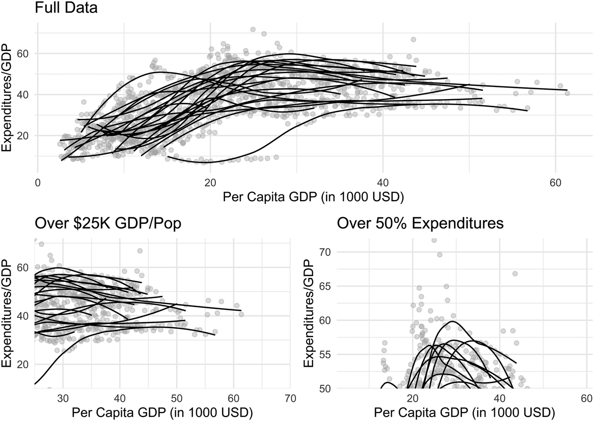
Figure 1 plots the relationship between expenditures as a share of GDP and per capita GDP for all countries in our sample. Each data point is represented with a gray dot and a Loess line is drawn for each country. Individual plots for each country are included in Appendix 1.

Figure 1.

Expenditures and per capita GDP

While there certainly appears to be a positive association in aggregate, only a few countries reveal this association continuing past the 25 thousand USD per capita GDP mark. Further, the only countries showing a positive trend at higher levels of per capita GDP are in the middle range of the expenditure measure. Every single country with a trend line above the 50% expenditures mark displays a flip to a negative relationship. Figure 1 suggests Wagner's law may hold only (1) at relatively low levels of per capita GDP or (2) in countries with relatively low levels of state expenditures. Conversely, according to Figure 1, there is no support for Wagner's law at high levels of either per capita GDP or expenditures/GDP. In other words, Wagner's law is less likely to hold at higher levels of development and past certain levels of government expenditure.

Previous debates surrounding Wagner's law emerged as scholars questioned whether the variables were associated with each other or merely taking part in separate positive random walks. Henrekson (Reference Henrekson1993), for example, points out that the observed positive association between expenditures and per capita GDP in Sweden may be in fact be spurious. Our data suggest the two variables are not even positively associated over the entire period for most of our cases. The association does not even appear; thus, we are not concerned with the tests’ spuriousness or cointegration. We believe this is evidence sufficient for falsification of Wagner's law.

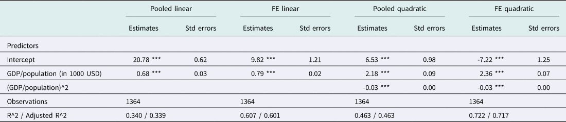
To demonstrate the robustness of this result we fit statistical models. We fit pooled ordinary least squares models and fixed effects (FE) models, which allow the intercepts to vary for each country. Including FEs allows us to account for time-invariant omitted variables specific to each country. Both linear and quadratic models are fitted. The results are presented in Table 1.

The linear model suggests a significant positive association between the expenditure share (government expenditures/GDP) and per capita GDP. The coefficient in this first model suggests that a 1 thousand USD increase in per capita GDP is associated with an increase of 0.68 percentage points in expenditures as a share of GDP. The second column shows the linear model with country-level FEs and shows a similar relationship; a 1,000 USD increase in per capita GDP is associated with a 0.78 percentage point increase in expenditures/GDP (country intercepts are not shown in Table 1). This test supports Wagner's law, however, forcing the relationship to take a linear form is inconsistent with the actual patterns in the data shown in Figure 1. The overall pattern appears relatively flat at lower levels of development, increases in the middle of the range, and decreases at higher levels. Thus, the next two models allow the relationship to take a non-linear form.

Table 1.

Linear and quadratic models: pooled and with fixed effects

* p < 0.05 ** p < 0.01 *** p < 0.001

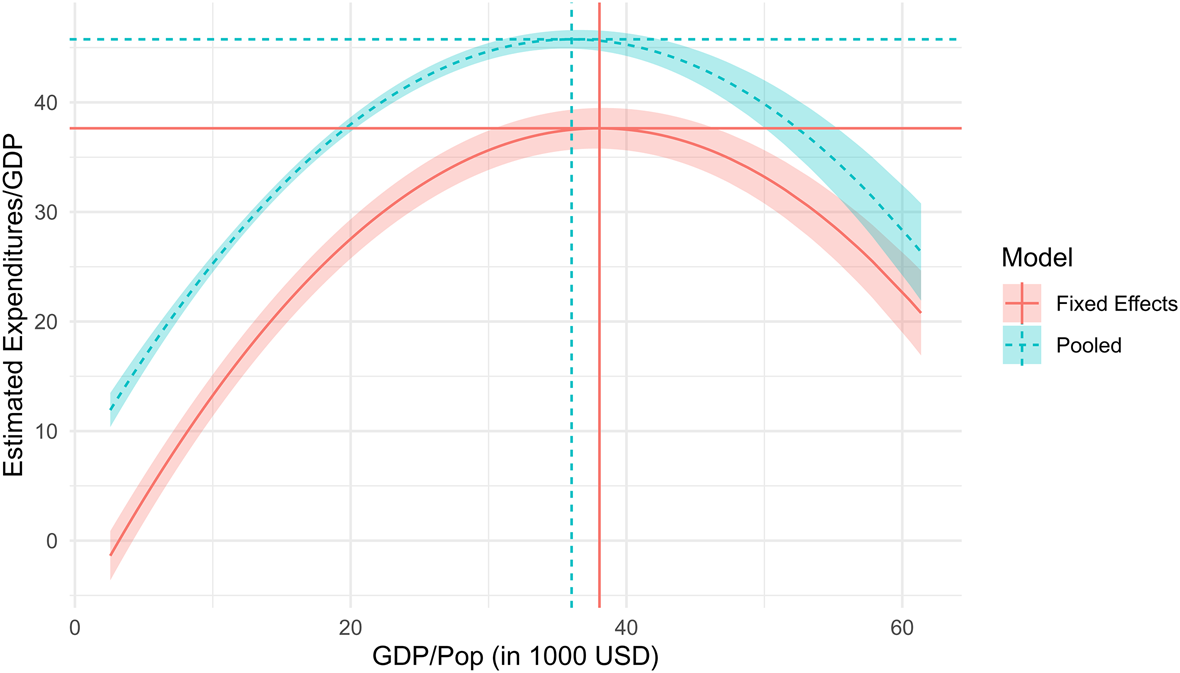
The pooled model shows that the non-linear quadratic relationship between the two variables is significant. The same is true for the quadratic model with country-level fixed effects. In both the pooled and FE models, the relatively higher R-squared means that the quadratic models explain more of the variation than the linear models. From the pooled and FE quadratic models (the 3^rd and 4^th columns in Table 1), we plot the estimated expenditures/GDP over the range of per capita GDP in our data in Figure 2.

Figure 2.

Pooled and FE quadratic model estimates

With these model estimates we can calculate the inflection point: the point at which the relationship switches from positive to negative, for the overall model (the best representation of all cases). We do this by setting the first derivative of the equation to zero and solving the equation. These lines are plotted for each of the models in Figure 2. Using the FE model coefficients from Table 1, the calculated point of inflection is 38,000 USD, which corresponds to an estimated expenditure level of 37.6% of GDP. The pooled inflection point and corresponding estimated expenditure level are 36, 000 USD and 45.8% of GDP. The corresponding estimated expenditure levels differ, but the inflection points are very similar levels of per capita GDP.

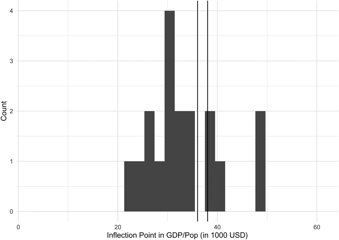
We also calculate inflection points for each country (see the appendix for plots of each country with calculated inflection plots). We fit linear and quadratic models and choose the specification with better explanatory power (according to the R-squared calculation). This prevents us from identifying an inflection point in cases where a linear model is a better representation – where Wagner's law still holds, such as in Japan and Spain. Also, we do not consider inflection points calculated beyond the range of observable GDP per capita for a specific country. This is the case for France and Turkey. The maximum GDP per capita in these four countries are 19.5 thousand USD in Turkey, 35.1 in Spain, 36.3 in Japan, and 37.9 in France. Only France exceeds the overall FE model inflection point of 37.6 thousand USD, and only it and Spain exceed the overall pooled model inflection point of 36.0 thousand USD. France is the only one of these four countries to exceed an expenditure level of 50% of GDP.

The inflection points for the remainder of our cases, along with the inflection points from the full pooled and FE models, are presented in a histogram in Figure 3. The country-specific inflection points range from 23.1 in Portugal to 49.5 in Switzerland.

Figure 3.

Histogram of country-specific inflection points

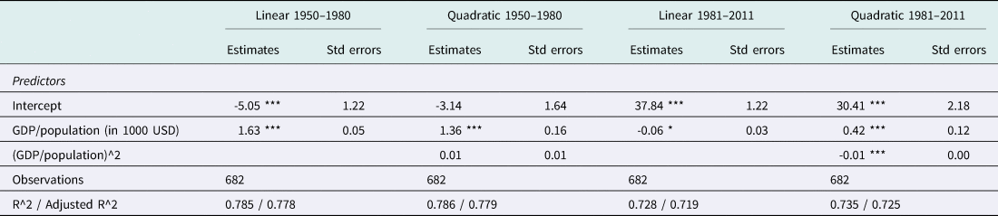
The evidence presented above demonstrates that Wagner's law has limits at higher levels of economic development, but we still want to see how it holds up in different time periods. Durevall and Henrekson (Reference Durevall and Henrekson2011) show that Wagner's law doesn't hold up well after the 1970s in Sweden or the UK, and Lamartina and Zaghini (Reference Lamartina and Zaghini2011: 151) find that it doesn't work after 1990. Here we see if that proposition is also true for the countries in our sample. We split the data into two sets according to the year of observation: 1950–1980 and 1981–2011. We use linear and quadratic FE models. The results for the two models are presented in Table 2.

Table 2.

FE Linear and quadratic models for two periods

* p < 0.05 ** p < 0.01 *** p < 0.001

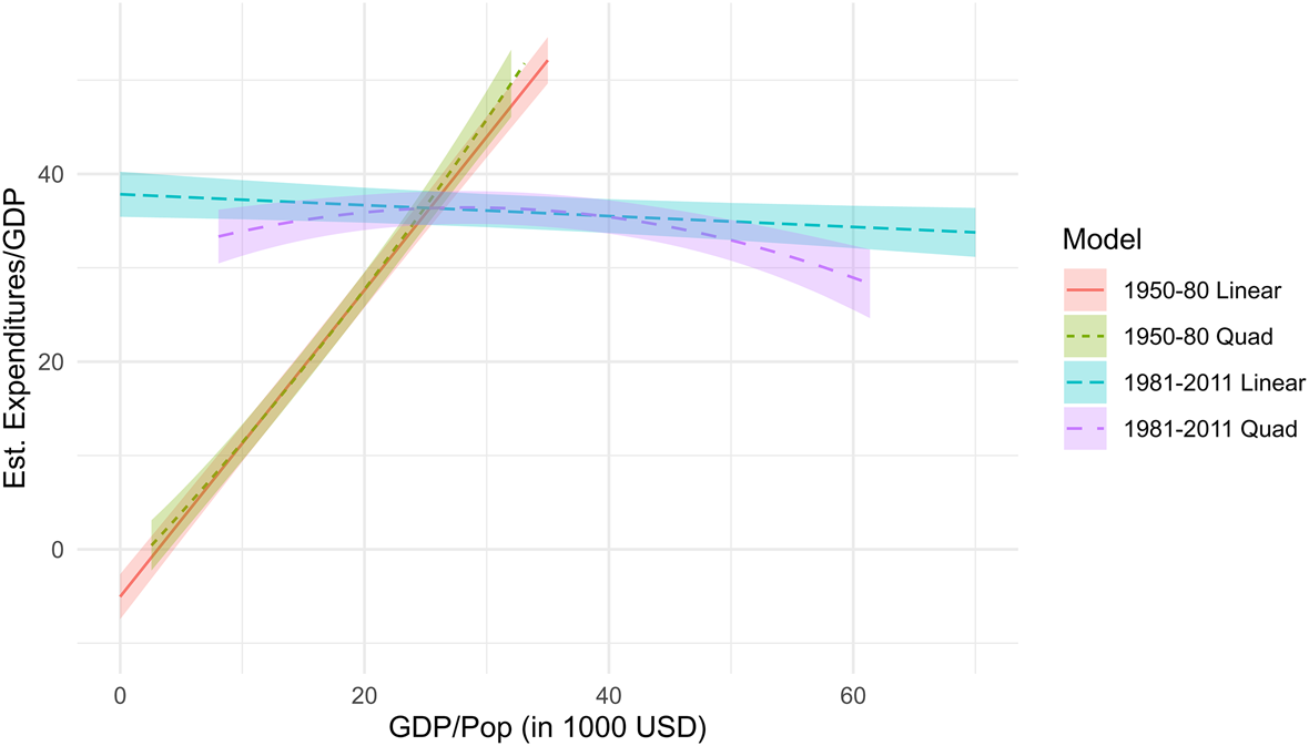
The first column in Table 2 shows that in the first half of the period the linear association between our two variables is positive and significant. The coefficient for the first period, 1.63, is significantly larger than the coefficient for the entire period (0.79). The positive association in the earlier period offers strong support for Wagner's law. In the later period, however, the coefficient switches to a small but negative estimate of -0.06. This means the finding from Durevall and Henrekson (Reference Durevall and Henrekson2011) that the relationship doesn't hold after the 1970s also seems to be true in our much larger sample of countries. The estimates from the two periods, both linear and quadratic, are plotted in Figure 4. The quadratic model in the second period also suggests a realtively flat, or even negative, relationship.

Figure 4.

Model Estimates for the two periods

This section shows that Wagner's law has important scope conditions. Forcing the relationship to take a linear form can generate misleading findings that support the Law, but allowing flexibility in the model by adding a polynomial term dramatically improves model fit. At higher levels of per capita GDP, the relationship flips from positive to negative. There may be an expenditure “ceiling” that nations are unlikely to surpass. We also identify the temporal scope conditions of the law. It works well in all cases (in the linear model) during the first half of our period (1950–1980) but not in the second (1981–2011). Consistent with other studies, we find that the law is less likely to apply in more recent periods.

5. Why Wagner's law failed: the relationship between taxation and spending

Our basic argument is simple: limits on state spending are caused by limits on taxation. From a rational choice perspective, this should sound obvious – of course the size of the state will ultimately be constrained not by resistance to the benefits it provides via state spending but by opposition to the costs it imposes in the form of taxes. Thus, although Wagner's law is about state spending, its eventual failure cannot be understood without analyzing taxation, and the relationship between taxation and spending.

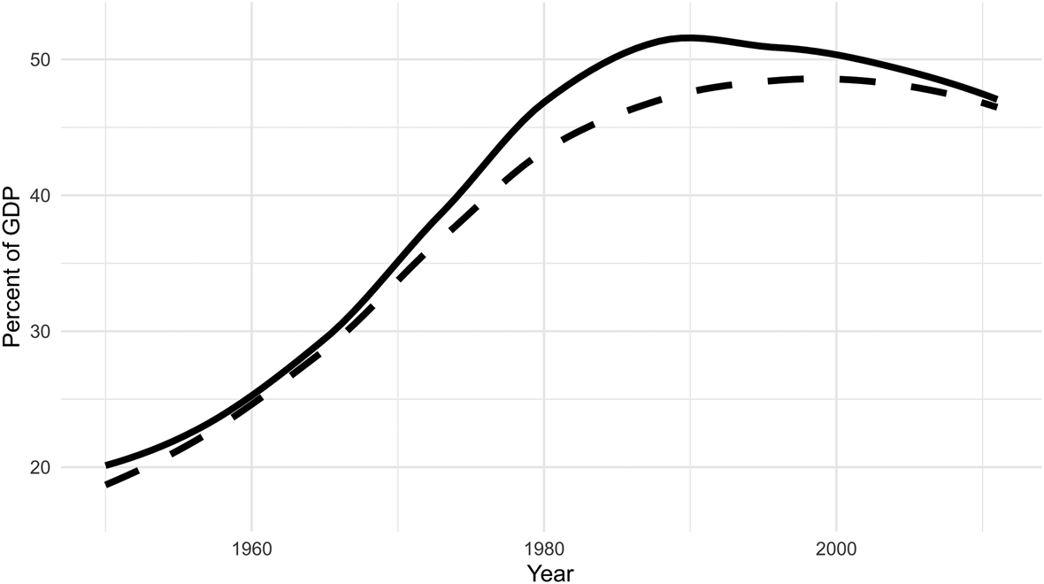
Figure 5 shows the relationship between spending (solid line) and revenue (dashed line) for high-expenditure countries (Austria, Belgium, Canada, Denmark, Finland, France, Germany, Ireland, Italy, Netherlands, Norway, Sweden, and the United Kingdom). It shows that the high-spending counties hit a ceiling on further growth around the late 1980s. Since that point, both spending and revenue have decreased. Until the late 1960s, spending and revenues were very closely linked. They diverged sharply from that point until about 2000, when revenues and spending again come close to converging. This suggests that deficits and the debt they produce will be an important part of the timing of the ceiling on state growth (although perhaps not in the United States; see Prasad, Reference Prasad2018).

Figure 5.

Expenditures (solid line) and revenues (dashed line) for “high-spending” countries

The relationship between taxation and spending is complicated. On an annual basis, spending is only weakly constrained by taxation, as states can borrow or find non-tax sources of short-term revenue, such as selling state assets. However, taxation sets general, long-term constraints on spending, working via what we call “rubber band” causation – spending can be stretched beyond revenue, but only so far and only for so long, until it is pulled back, in one way or another. Wagner's law stopped working because states at the highest levels of taxation found it difficult to increase taxes further. They could only continue to grow by running deficits, but this led to increasing state debt, which eventually pulled spending down. The rubber band could only stretch so far.

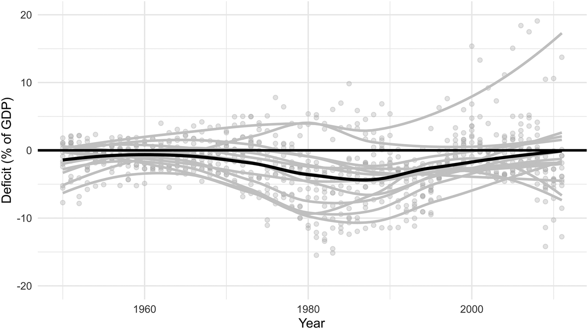
Figure 6 illustrates this “rubber band” causation for high-expenditure countries. The plot includes a line for each country and a dark Loess line for the entire sample. Deficits were very low in these countries from 1950 until about 1965, and during this period surpluses were not uncommon. From roughly 1965 until 1985, deficits were increasing and very high. This is the period when deficit spending began to replace taxation as a way of funding state spending. After about 1985 annual deficits began to decease, but they remained high until around 2000 (total state debt in high-expenditure countries peaks at that time). High-expenditure states used deficits to continue increasing spending for a few decades, but due to increasing state debt this was only a short-term postponement of the inevitable. The inability of states to continue increasing tax revenues eventually limited state spending and the overall growth of the state.Footnote ⁶

Figure 6.

Deficits for “high spending” countries

Two important questions remain: (1) Why have contemporary states, especially those at high levels of taxation, found it difficult to continue increasing their tax revenue?, and (2) What are the mechanisms by which increasing state debt eventually limits spending?

The first main limitation on taxation in high-tax states is a product of their tax structure. High-tax states tend to rely mainly on regressive indirect consumption taxes, as opposed to the progressive direct income taxes that are dominant in low-tax states like the US (Kiser and Karceski, Reference Kiser and Karceski2017: 83; Prasad, Reference Prasad2018).Footnote ⁷ A reliance on regressive indirect taxes facilitated the growth of high-tax states up to a point (Beramendi and Rueda, Reference Beramendi and Rueda2007), but it is now responsible for limiting their further growth. The reason is simple: unlike progressive taxes on the rich, high regressive taxes on the working and middle classes will eventually begin to threaten their basic standard of living (Martin and Gabay, Reference Martin and Gabay2012; Wagner Reference Wagner1883).Footnote ⁸ Direct tax rates on the rich have in several cases exceeded 50%, but rates anywhere near that high for regressive indirect taxes are unimaginable in a democratic context.Footnote ⁹ High-expenditure states seem to have reached a limit of indirect tax rates. In the last few decades, VAT rates have peaked between 20–25% within the OECD.

If states can't continue to increase regressive indirect taxes, what about increasing direct taxes on capital or the wealthy? Let's look first at taxes on capital. When globalization decreased the cost of capital mobility, some predicted a “race to the bottom” for taxes on capital (Rodrik, Reference Rodrik1997), but that has not happened (Campbell, Reference Campbell2004; Ganghof and Genschel, Reference Ganghof and Genschel2008; Garrett and Mitchell, Reference Garrett and Mitchell2001; Swank and Steinmo, Reference Swank and Steinmo2002).Footnote ¹⁰ Although the literature has stressed the fact that tax rates on capital have not fallen substantially, for our purposes it is important to stress that they have not increased either (Hays, Reference Hays2003), suggesting that the decreased cost of capital mobility has had some limiting effect on a state's ability to tax capital.

Progressive income taxes on the wealthy have also been difficult to increase, for several reasons. First, the rich have opportunities to avoid and evade taxes by moving assets across national borders in ways that working-class taxpayers cannot (Sharman, Reference Sharman2006; Zucman, Reference Zucman and Fagan2015), so countries relying more on taxing the rich will get less net tax revenue (Lockhart, Reference Lockhart2003; Prasad, Reference Prasad2012: 170). Second, highly progressive tax systems promote and reinforce adversarial class relations, which result in lower revenue (Beramendi and Rueda, Reference Beramendi and Rueda2007; Prasad, Reference Prasad2006). Third, and part of this adversarial fiscal culture, Martin (Reference Martin2013) has shown that policy proposals to increase progressivity are often met by resistance from the rich,Footnote ¹¹ and that these “rich people's movements” are often successful in blocking progressivity. Finally, Scheve and Stasavage (Reference Scheve and Stasavage2016) note that the causal mechanism responsible for the initial rise of progressivity, mass conscription for war, is unlikely to occur again in the era of highly mechanized warfare. For all of these reasons, progressive income taxation will be hard to increase.

It is currently difficult for states, especially high-tax states, to increase both indirect and direct taxes. This leaves them with only one option if they want to continue to increase spending, to run budget deficits. The main problem with deficits is that they increase the legitimacy of the state in the short term but decrease it in the long run. As the theory of quasi-voluntary compliance (Levi, Reference Levi1988) suggests, the legitimacy of the state is in part a function of whether people think they are getting benefits commensurate to the costs they pay in taxes. In the short run, deficit spending allows rulers to provide more benefits than costs, increasing their legitimacy, because total taxation is less than total spending citizens are getting more than they paid for. However, as annual deficits accumulate into debt that has to be paid off (at the very least, the interest on the debt must be paid), people will be getting less from state spending than they are paying in taxes (because some of their tax payments go to paying off, or at least servicing, the debt). This will necessarily threaten the legitimacy of states. It also facilitates the rise of anti-tax, anti-state parties, because they can make a compelling argument that the state is inefficient and irresponsible – that it is not providing benefits via spending commensurate to the costs of taxes.Footnote ¹²