1 Introduction
Entrainment can be described as the assimilation and mixing process of low-vorticity fluid by neighbouring high-vorticity fluid along a low-to-high vorticity interface (LHVI). The LHVI is typically referred to as the turbulent–non-turbulent interface, or TNTI, in turbulent flows, but is here referred to as the LHVI to extend the concept to laminar flows. Using observations on a jet, Corrsin & Kistler (Reference Corrsin and Kistler1955) proposed that the LHVI possesses a finite thickness, across which sharp spatial gradients in enstrophy, velocity and Reynolds stresses should be observed. The transfer of enstrophy occurs along the LHVI at scales on the order of the Kolmogorov length scale. This model for the LHVI has been verified in jets (Wolf et al. Reference Wolf, Holzner, Krug, Lüthi, Kinzelbach and Tsinober2013; Mistry et al. Reference Mistry, Philip, Dawson and Marusic2016), in canonical turbulent boundary layers (Phillip & Marusic Reference Phillip and Marusic2012; Chauhan et al. Reference Chauhan, Philip, de Silva, Hutchins and Marusic2014) and in stratified flows (Krug et al. Reference Krug, Holzner, Lüthi, Wolf, Kinzelbach and Tsinober2013). Despite entrainment occurring at smaller scales, large-scale motions play an important role as well. Specifically, larger scales within the high-vorticity region act to ‘roll-up’ irrotational fluid in a swirling manner towards the LHVI (Brown & Roshko Reference Brown and Roshko1974; Dimotakis & Brown Reference Dimotakis and Brown1976). Although the classical description of roll-up is not observed in jets or boundary layers, larger eddies along the periphery do act to draw irrotational fluid in contact with the LHVI, which is then consumed by smaller scales (Phillip & Marusic Reference Phillip and Marusic2012; Chauhan et al. Reference Chauhan, Philip, de Silva, Hutchins and Marusic2014; Mistry et al. Reference Mistry, Philip, Dawson and Marusic2016). This roll-up mechanism is very apparent in laminar starting vortices, where irrotational fluid is spiralled towards the vortex-core centre (Olcay & Krueger Reference Olcay and Krueger2008, Reference Olcay and Krueger2010). However, since vorticity in laminar vortex rings can only be exchanged via laminar diffusion, this roll-up mechanism may not be representative of the entrainment mechanism observed in turbulent vortex rings.
In many of the aforementioned studies, the stationarity condition allowed for the entire LHVI to be treated as a single data ensemble, from which statistics could be extracted. Similar statistical analyses are not meaningful when studying non-stationary shear layers that are spatially non-similar and dependent on flow history. In spite of this challenge, non-stationary shear layers are ubiquitous. For example, any accelerating body will unavoidably form an non-stationary shear layer in its wake. As such, the non-stationarity of the shear layer is inseparably linked to the development of starting vortices, and therefore to the propulsion for instance of swimmers and flyers. Environments where the flow conditions vary with time, such as atmospheric and cardiovascular flows, will also exhibit non-stationary shear layers (Gharib, Rambod & Shariff Reference Gharib, Rambod and Shariff1998; Pawlak & Armi Reference Pawlak and Armi1998).
In spite of their ubiquity, the mixing and entrainment mechanics of non-stationary shear layers remain poorly understood. Previous studies on the subject have typically focused on the development of starting vortices formed by piston–cylinder arrangements. Earlier studies have considered the effect of the piston stroke length to diameter ratio (Dabiri & Gharib Reference Dabiri and Gharib2004; Shadden, Dabiri & Marsden Reference Shadden, Dabiri and Marsden2006; Shadden et al.
Reference Shadden, Katija, Rosenfeld, Marsden and Dabiri2007), as well as the piston’s velocity program (Olcay & Krueger Reference Olcay and Krueger2008, Reference Olcay and Krueger2010). Xu & Nitsche (Reference Xu and Nitsche2015) specifically explored the effect of acceleration rate on starting-vortex development through numerical simulations of an accelerating plate travelling at a velocity
 $U=at^{p}$
. Here,
 $a$
represented an acceleration constant while
 $p$
was set to 0.5, 1 and 2. The results showed that after an initial viscous stage of short duration
 $(s/D<0.03)$
, the dynamics of the vortex, including the circulation and the position of its vortex centre, agreed well with inviscid scaling. Although these studies represent significant contributions, they are limited in their applicability. For one, all the studies in question investigated starting vortices within a laminar regime. Secondly, the studies did not comment on the role of Kelvin–Helmholtz (KH) instabilities. For instance, the KH instabilities in stratified, laminar shear layers accelerating through contracting channels have been observed to detach and merge with downstream instabilities, (Caulfield, Yoshida & Peltier Reference Caulfield, Yoshida and Peltier1996) or even ‘leapfrog’ past them (Pawlak & Armi Reference Pawlak and Armi1998, Reference Pawlak and Armi2000). However, the applicability of these studies on laminar, accelerating shear layers to situations involving higher accelerations, as well as to transitional and turbulent regimes, is not certain.
The complex topology of a turbulent shear layer must intuitively affect the transport of vorticity-containing mass and circulation into the starting vortex, which will be studied here as a canonical non-stationary case. A shear layer’s topology must also alter the entrainment and vorticity diffusion that occurs at the LHVI. LHVI topology and mechanics at higher Reynolds numbers have been studied extensively for various ergodic flows. Work by da Silva, Dos Reis & Pereira (Reference da Silva, Dos Reis and Pereira2011) demonstrated that the topology and entrainment mechanics along an LHVI can be attributed to intense vortical structures that exist just beneath the shear layer’s surface. Further to this, Wolf et al. (Reference Wolf, Holzner, Krug, Lüthi, Kinzelbach and Tsinober2013) demonstrated that the entrainment rate is greater at positions along an LHVI that are concave relative to the irrotational fluid. Although these findings are compelling, their pertinence towards the LHVIs of non-stationary shear layers is uncertain.
Towards understanding the entrainment and associated topology of non-stationary shear layers, the current study considers a canonical, non-stationary problem: A constantly accelerating circular plate of diameter
 $D$
towed normal to its path from rest. Here, acceleration is normalized as
 $a^{\ast }=aD^{3}/\unicode[STIX]{x1D708}^{2}$
, where
 $\unicode[STIX]{x1D708}$
is kinematic viscosity. Given the lack of work done on accelerating shear layers, one must abstract from conclusions of stationary flows to formulate a hypothesis. Firstly, visualizations of stationary shear layers (Brown & Roshko Reference Brown and Roshko1974; Dimotakis & Brown Reference Dimotakis and Brown1976), steady cylinder wakes (Cantwell & Coles Reference Cantwell and Coles1983) and turbulent boundary layers (Schlatter et al.
Reference Schlatter, Li, Brethouwer, Johansson and Henningson2010) demonstrate that increases in the Reynolds number results in increased turbulent mixing. This increased turbulent mixing has been demonstrated to correlate with an increase in the local entrainment rate along the LHVIs of these flows (Ricou & Spalding Reference Ricou and Spalding1961; Chauhan et al.
Reference Chauhan, Philip, de Silva, Hutchins and Marusic2014). The most compelling evidence of this is work presented in Wolf et al. (Reference Wolf, Holzner, Krug, Lüthi, Kinzelbach and Tsinober2013), which demonstrates that the entrainment rate increases along the periphery of a jet with increasing Reynolds number. An increase in turbulent mixing with increasing Reynolds number is also apparent in isolated vortex rings, which manifests in the form of azimuthal waves. Upon exceeding a circulation-based Reynolds number of
 $2\unicode[STIX]{x1D6E4}/\unicode[STIX]{x1D708}\sim O(10^{4})$
, a circular vortex ring will begin to tilt and stretch along its filament to facilitate the formation of azimuthal instability waves (Glezer Reference Glezer1988). The number of azimuthal waves that appear along the filament has been shown to increase with increasing Reynolds number (Liess & Didden Reference Liess and Didden1976; Didden Reference Didden1977; Saffman Reference Saffman1978). Based on what has been observed in stationary flow fields and isolated vortex rings, it is hypothesized that by increasing
 $a^{\ast }$
, and therefore the instantaneous Reynolds number, that the shear layer will exhibit greater turbulent mixing and thus an increased entrainment rate. This hypothesis assumes that the shear layer has long transitioned into the turbulent regime. For this reason, sufficiently large
 $a^{\ast }$
values have been selected for the experiments presented herein. To validate this hypothesis, visualizations and planar measurements along the plate’s midspan were performed. The experiments are therefore chosen to elucidate the effect that accelerating flows have on shear-layer topology and entrainment, and are outlined in the following section.
2 Experimental set-up
A circular plate of diameter
 $D=30~\text{cm}$
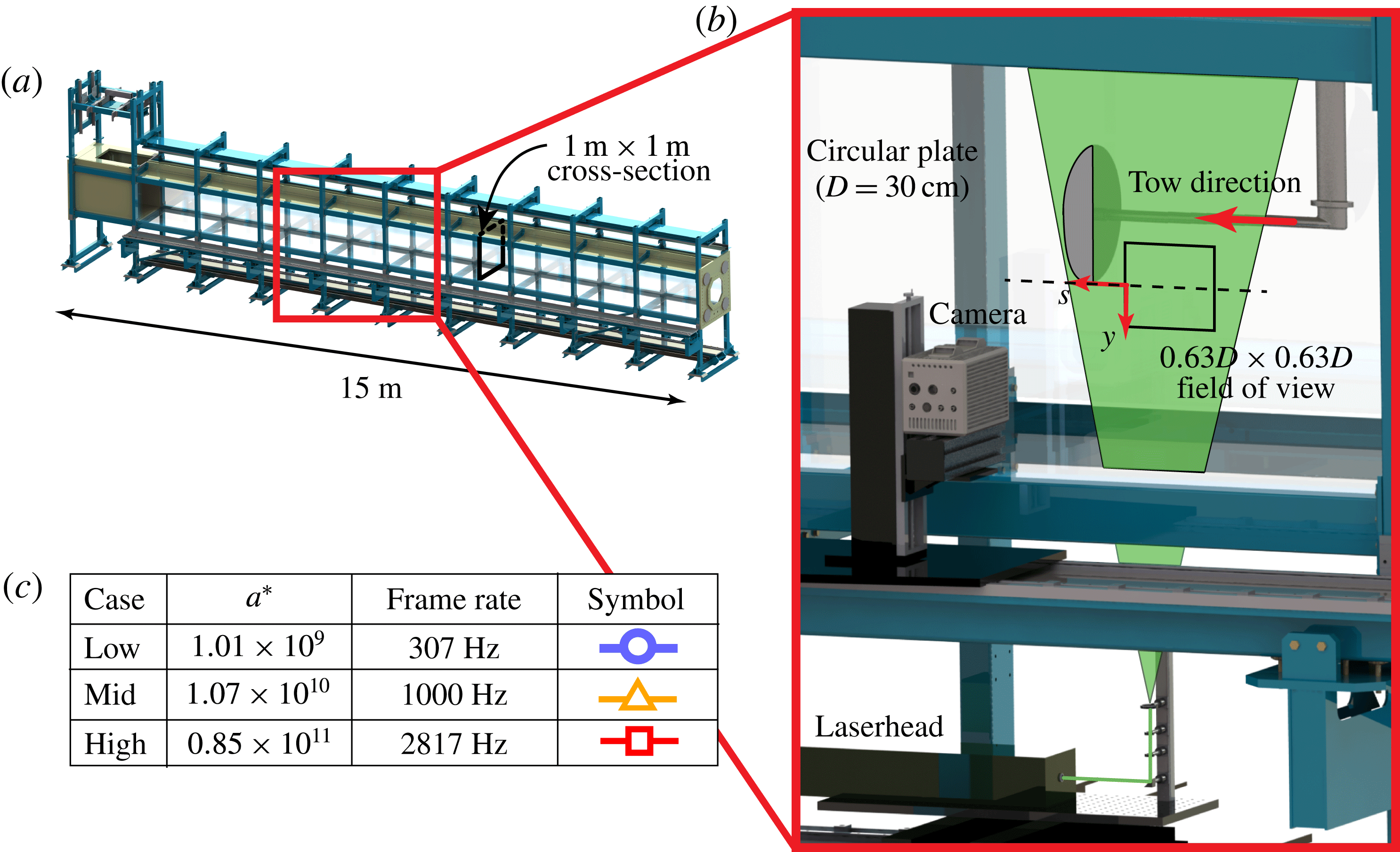
was continuously accelerated through a 15 m-long, optical towing tank (figure 1
a) with a square cross-sectional area of
 $1~\text{m}^{2}$
, resulting in a blockage ratio of 7 %. The plate was mounted to a traverse located above the tank via a sting that attached to the plate’s suction side. The sting’s diameter and horizontal length were
 $0.1D$
and
 $2D$
, respectively. Three
 $a^{\ast }$
values spanning three orders of magnitude were tested. Their exact
 $a^{\ast }$
values are presented in figure 1(c). The current work hereafter refers to the experimental cases where
 $a^{\ast }=O(10^{9})$
,
 $O(10^{10})$
and
 $O(10^{11})$
as the low-, mid- and high-acceleration cases, respectively.
Shear-layer dye visualizations for the low- and mid-acceleration cases were performed over a domain of
 $0\leqslant s/D\leqslant 4.3$
, where
 $s$
is distance travelled. For either acceleration case, the shear layer exhibited a consistent topology throughout the entire
 $s/D$
domain. As such, particle image velocimetry (PIV) measurements were limited to
 $0.68\leqslant s/D\leqslant 1.05$
, which provided sufficient spatial resolution of the shear layer, yet was early enough that the starting vortex could be captured within the field of view (FOV). Thirty trials of PIV data were collected for each acceleration case. The PIV apparatus is shown in figure 1(b). A 40 mJ-per-pulse laser was expanded into a 1 mm-thick sheet that illuminated a
 $0.63D\times 0.63D$
planar FOV.
 $55~\unicode[STIX]{x03BC}\text{m}$
polymer microspheres were added to the water to serve as tracer particles. Images centred at the plate’s bottom edge were captured by a high-speed camera at frame rates indicated in figure 1(c), which maintained equal temporal resolution between acceleration cases. The images were flipped vertically so that the
 $y$
axis would point upwards, and subsequently processed in DaVis 8.2.0 to extract velocity fields. A multi-pass interrogation scheme was applied. Two initial passes were performed using 128-by-128-pixel interrogation windows with 75 % overlap, followed by two final passes performed using 64-by-64-pixel interrogation windows with 75 % overlap. Thus, the final vector field was comprised of 256 by 256 vectors. Vectors with peak ratios less than 2.0 were identified as outliers (Hain & Kaehler Reference Hain and Kaehler2007). These outliers, which comprised on average 2 % of all vectors, were replaced using neighbouring vectors. Finally, a
 $3\times 3\times 3$
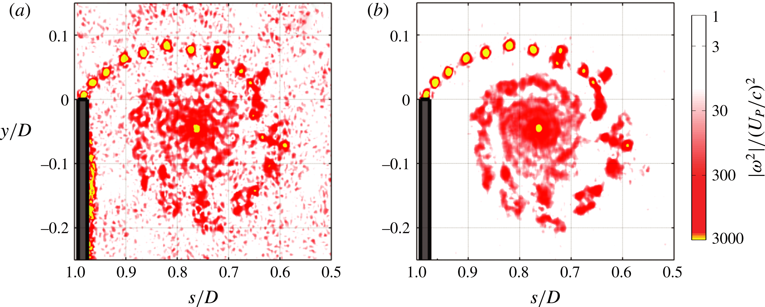
, three-dimensional Gaussian filter was applied on the enstrophy fields to reduce the high-frequency noise in the enstrophy field. Representative enstrophy contours from the mid-acceleration case before and after applying the Gaussian filter are presented in figure 2, demonstrating that the filtering has little effect on the structures within the starting vortex itself. Subsequent data processing was performed in MATLAB 2012a.
Summary of the experimental apparatus: (a) a circular plate was accelerated through a 15 m-long towing tank with a
 $1~\text{m}\times 1~\text{m}$
square cross-section; (b) images were captured within a
 $0.63D\times 0.63D$
planar FOV using the presented optical apparatus; (c) tested
 $a^{\ast }$
values, camera frame rates, and symbols to be used in subsequent plots.

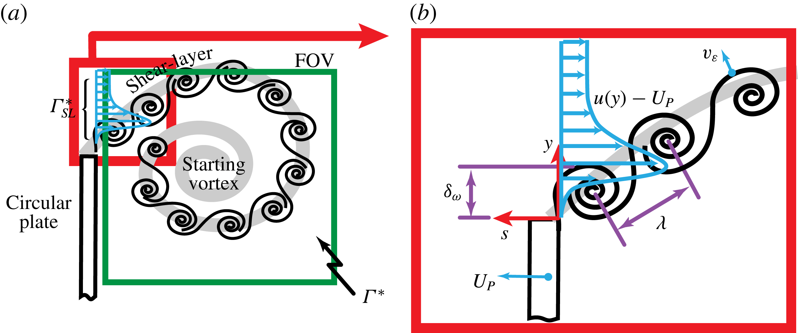
Figure 3(a,b) illustrates the experiment and summarizes the quantifiable measures derived from the PIV measurements. The circular plate travels left at an instantaneous velocity of
 $U_{P}$
. The shear layer is comprised of KH instabilities and exhibits a global velocity profile of
 $u(y)$
at the plate edge. The starting-vortex circulation (
 $\unicode[STIX]{x1D6E4}^{\ast }$
) is determined via an area integral of vorticity that spans the section of the FOV located behind the plate. The circulation provided by the shear layer (
 $\unicode[STIX]{x1D6E4}_{SL}^{\ast }$
) is calculated by integrating the vorticity flux across a line spanning from the plate edge to the top of the FOV (
 $y_{top}$
). The initial starting-vortex circulation is then added (
 $\unicode[STIX]{x1D6E4}_{0}^{\ast }$
) so that
 $\unicode[STIX]{x1D6E4}^{\ast }$
and
 $\unicode[STIX]{x1D6E4}_{SL}^{\ast }$
may be directly compared.
 $\unicode[STIX]{x1D6E4}_{SL}^{\ast }$
represents the aggregate spanwise vorticity generated by the shear layer, while
 $\unicode[STIX]{x1D6E4}^{\ast }$
represents the amount of spanwise vorticity within the starting vortex that has not tilted out of plane. Both
 $\unicode[STIX]{x1D6E4}^{\ast }$
and
 $\unicode[STIX]{x1D6E4}_{SL}^{\ast }$
are normalized here by
 $U_{P}D$
:
 $$\begin{eqnarray}\unicode[STIX]{x1D6E4}^{\ast }=\frac{1}{U_{P}D}\iint \unicode[STIX]{x1D714}\,\text{d}A,\quad \unicode[STIX]{x1D6E4}_{SL}^{\ast }=\frac{1}{U_{P}D}\int _{0}^{t}\int _{0}^{y_{top}}\unicode[STIX]{x1D714}(u(y)-U_{P})\,\text{d}y\,\text{d}\unicode[STIX]{x1D70F}+\unicode[STIX]{x1D6E4}_{0}^{\ast }.\end{eqnarray}$$
When calculating
 $\unicode[STIX]{x1D6E4}_{SL}^{\ast }$
, the integral is evaluated along an axis that runs parallel to the plate, positioned at the suction side of the plate’s tip.
Representative normalized enstrophy contours (a) before and (b) after applying a
 $3\times 3\times 3$
, three-dimensional Gaussian filter to the enstrophy field. The filter removes high-frequency noise within the field, while maintaining the structures within the vortex.

To characterize entrainment, the entrainment velocity (
 $v_{\unicode[STIX]{x1D700}}$
) was calculated along LHVIs that were identified via various
 $|\unicode[STIX]{x1D714}^{2}|$
thresholds.
 $v_{\unicode[STIX]{x1D700}}$
represents the relative velocity of the local enstrophy isosurface in a Lagrangian frame (Wolf et al.
Reference Wolf, Holzner, Krug, Lüthi, Kinzelbach and Tsinober2013).
 $v_{\unicode[STIX]{x1D700}}$
is normal to the
 $|\unicode[STIX]{x1D714}^{2}|$
contour and positive in the direction of increasing
 $\unicode[STIX]{x1D735}|\unicode[STIX]{x1D714}^{2}|$
. Thus, negative and positive
 $v_{\unicode[STIX]{x1D700}}$
values indicate entrainment and detrainment, respectively:
 $$\begin{eqnarray}v_{\unicode[STIX]{x1D700}}=\left.-\frac{\text{D}|\unicode[STIX]{x1D714}^{2}|}{\text{D}t}\right/|\unicode[STIX]{x1D735}|\unicode[STIX]{x1D714}^{2}||.\end{eqnarray}$$
It is commonly accepted that
 $v_{\unicode[STIX]{x1D700}}$
is sensitive to the
 $|\unicode[STIX]{x1D714}^{2}|$
threshold, and that there is no objective way in selecting it (Wolf et al.
Reference Wolf, Holzner, Krug, Lüthi, Kinzelbach and Tsinober2013). The current study determines a threshold per time step by increasing it from zero by increments of
 $0.005\times \max (|\unicode[STIX]{x1D714}^{2}|)$
until the area of the rotational region changes by less than a certain percentage. Thresholds of 1 %, 2 % and 4 % area change (
 $\unicode[STIX]{x0394}A$
) were used and their results were compared. To calculate a two-dimensional analogue for the entrainment rate, the entrainment velocity was integrated along the entire periphery of the identified LHVI using the following discrete integral:
 $$\begin{eqnarray}\unicode[STIX]{x1D700}=-\oint _{LHVI}v_{\unicode[STIX]{x1D700}}\,\text{d}s\equiv -\sum v_{\unicode[STIX]{x1D700}}\unicode[STIX]{x0394}s.\end{eqnarray}$$
Here,
 $v_{\unicode[STIX]{x1D700}}$
is summed along the entire LHVI while being multiplied by
 $\unicode[STIX]{x0394}s$
, which represents the length of the LHVI corresponding to the current data node. For each acceleration case,
 $\unicode[STIX]{x1D700}$
is normalized by
 $U_{P}D$
, compiled into a single ensemble across all 30 runs, and then averaged. This global average, referred to hereafter as
 $\overline{\unicode[STIX]{x1D700}/(U_{P}D)}$
, produced consistent results when comparing acceleration cases at equal area thresholds. Although the global average cannot provide temporal trends, it can be reliably determined since it is calculated from the order of 1000 separate measurements.
Pertinent experimental parameters and quantifiable measures of the shear layer and starting vortex.
 $\unicode[STIX]{x1D6E4}^{\ast }$
represents the circulation within the starting vortex.
 $\unicode[STIX]{x1D6E4}_{SL}^{\ast }$
represents the integral circulation fed by the shear layer through the relative-velocity profile
 $u(y)-U_{P}$
.
 $\unicode[STIX]{x1D706}$
is a measure of the spacing between KH instabilities, while
 $T_{\unicode[STIX]{x1D714}}$
is the time period between consecutive sheddings.
 $\unicode[STIX]{x1D6FF}_{\unicode[STIX]{x1D714}}$
represents the shear-layer thickness and
 $v_{\unicode[STIX]{x1D700}}$
is the entrainment velocity, which is a measure of local enstrophy spreading.

The 30-run, phase-averaged
 $|\unicode[STIX]{x1D714}^{2}|$
-fields exhibited coherent and distinct KH instabilities near the plate tip, and as such were used to identify instances of KH-instability shedding, from which the shedding wavelength (
 $\unicode[STIX]{x1D706}$
) of KH instabilities was determined. These shedding instances coincided nearly exactly (
 $+/-$
frame) with instances where the shear-layer thickness (
 $\unicode[STIX]{x1D6FF}_{\unicode[STIX]{x1D714}}$
), as defined in Brown & Roshko (Reference Brown and Roshko1974), exhibited a local minimum:
 $$\begin{eqnarray}\unicode[STIX]{x1D6FF}_{\unicode[STIX]{x1D714}}=\max (|\unicode[STIX]{x1D714}|)^{-1}\int _{0}^{y_{top}}|\unicode[STIX]{x1D714}|\,\text{d}y.\end{eqnarray}$$
Similar to
 $\unicode[STIX]{x1D6E4}_{SL}^{\ast }$
, the integral in (2.4) is calculated along an axis that runs parallel to the plate, positioned at the suction side of the plate’s tip. The
 $y$
-axis in (2.4) should in fact point normal to the shear layer to account for the shear layer’s incline. However, given that the shear layer’s incline is equal and constant for all accelerations tested
 $(\unicode[STIX]{x1D703}=45^{\circ })$
, omitting the incline still allows for
 $\unicode[STIX]{x1D6FF}_{\unicode[STIX]{x1D714}}$
to be relatively compared for all three acceleration cases.
 $\unicode[STIX]{x1D706}$
was evaluated as the distance travelled by the plate between consecutive sheddings and normalized by the mean shear-layer thickness
 $(\overline{\unicode[STIX]{x1D6FF}}_{\unicode[STIX]{x1D714}})$
. The time between shedding (
 $T_{\unicode[STIX]{x1D714}}$
) was used in calculating a shear-layer thickness Strouhal number, which was evaluated as
 $St_{\overline{\unicode[STIX]{x1D6FF}}_{\unicode[STIX]{x1D714}}}=\overline{\unicode[STIX]{x1D6FF}}_{\unicode[STIX]{x1D714}}/(U_{P}T_{\unicode[STIX]{x1D714}})$
.
To characterize the instantaneous turbulence, a circulation-based Reynolds number calculated after Glezer (Reference Glezer1988) is presented throughout this study. It can be approximated from the kinematics of the circular plate using the following equation:
 $$\begin{eqnarray}Re_{\unicode[STIX]{x1D6E4}}=\frac{2\unicode[STIX]{x1D6E4}}{\unicode[STIX]{x1D708}}=\frac{2\displaystyle \int _{0}^{t}u(\unicode[STIX]{x1D70F})^{2}\,\text{d}\unicode[STIX]{x1D70F}}{\unicode[STIX]{x1D708}}=\sqrt{\frac{8as^{3}}{\unicode[STIX]{x1D708}^{2}}}.\end{eqnarray}$$
Glezer (Reference Glezer1988) reports that vortex rings produced from piston cylinders of infinite piston stroke-to-diameter ratios will transition to turbulence when
 $Re_{\unicode[STIX]{x1D6E4}}=O(10^{4})$
. This occurs for the three acceleration cases presented herein within a diameters-travelled domain of
 $0.10\leqslant s/D\leqslant 0.35$
. Thus, the PIV measurements and dye visualizations presented herein are assumedly turbulent.
3 Results
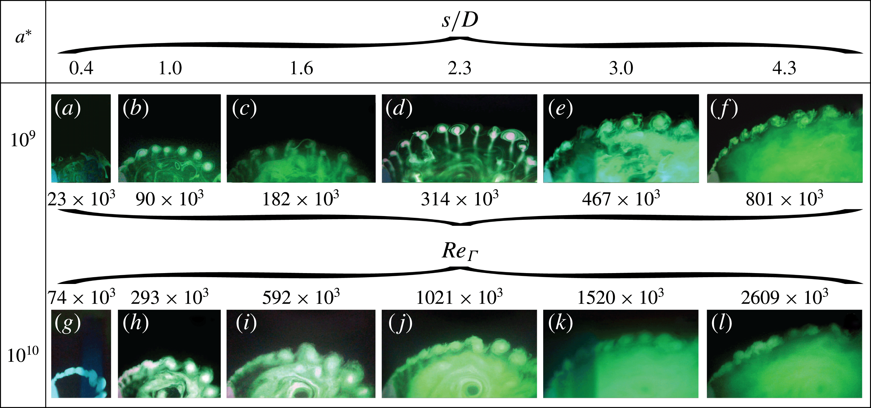
Figure 4 presents shear-layer dye visualizations for the low- and mid-acceleration cases, at various
 $s/D$
ratios and corresponding instantaneous
 $Re_{\unicode[STIX]{x1D6E4}}$
. For either case, and over the entire
 $s/D$
domain tested, the shear layer is comprised of a KH-instability train that wraps around the starting vortex. The development of the starting vortex collapses with distance travelled and therefore agrees with classical formation-number arguments (Gharib et al.
Reference Gharib, Rambod and Shariff1998). Given the consistent flow topology, the PIV measurements were limited to
 $0.68\leqslant s/D\leqslant 1.05$
for all three acceleration cases. Unlike in stationary shear layers, instabilities that form along the low-acceleration shear layer are prone to merging and leapfrogging. However, when comparing either case, it is observed that the mid-acceleration case presents with a more organized KH-instability train, whereas the instabilities in the low-acceleration case exhibit more inconsistent spacing and leapfrogging. These observations can be seen more clearly from supplementary movie 1 available at https://doi.org/10.1017/jfm.2016.716. This increased organization with
 $a^{\ast }$
runs contrary to the expectation that the shear layer would disorganize for higher instantaneous Reynolds numbers through increased mixing.
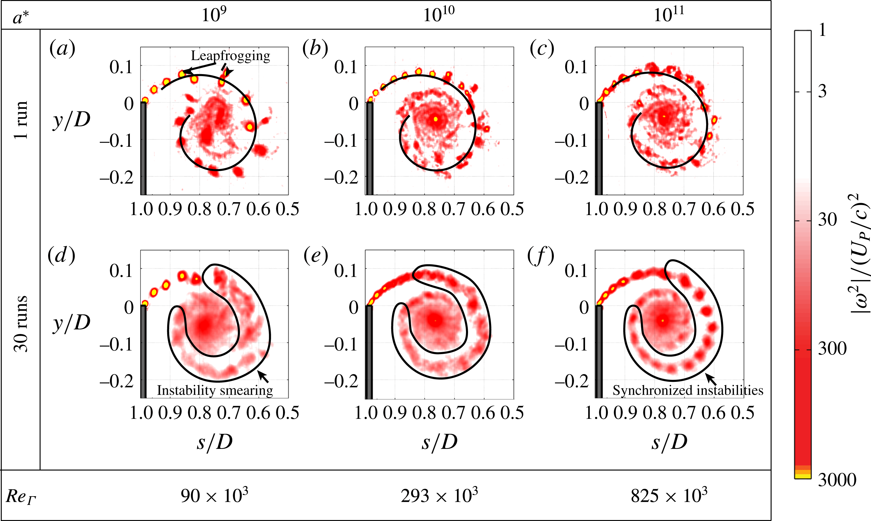
The reorganization of the flow with increasing
 $a^{\ast }$
can also be observed in all three accelerations from the
 $|\unicode[STIX]{x1D714}^{2}|$
fields presented in figure 5. From single trials of the low-acceleration case (figure 5
a), KH instabilities are observed to meander and leapfrog. These motions are subdued in the mid-acceleration case, and are essentially non-existent in the high-acceleration case. Instead, the KH instabilities adhere to a circular path. Further to this, the spacing and positioning of the instabilities become increasingly consistent with higher
 $a^{\ast }$
. This is apparent from the phase-averaged
 $|\unicode[STIX]{x1D714}^{2}|$
fields presented in figure 5(d–f). The KH instabilities in the low-acceleration case are smeared through phase averaging due to their stochastic motions. In contrast, the organization and synchronization of instabilities within the high-acceleration case results in their clear presence throughout the entire shear layer. Finally, the spacing between instabilities reduces with increasing
 $a^{\ast }$
. The reader is referred to supplementary movie 2, which presents additional sequences of single-run enstrophy fields, as well as the phase-averaged enstrophy fields.
Shear-layer dye visualizations for the low- and mid-acceleration cases at various
 $s/D$
. Corresponding instantaneous
 $Re_{\unicode[STIX]{x1D6E4}}$
are indicated as well. The complete visualization sequences can be viewed side-by-side in supplementary movie 1.

Single-run (first row) and phased-averaged (second row)
 $|\unicode[STIX]{x1D714}^{2}|$
fields at
 $s/D=1$
for all acceleration cases. Corresponding instantaneous
 $Re_{\unicode[STIX]{x1D6E4}}$
are indicated along the bottom row. Increasing
 $a^{\ast }$
organizes the vortex: KH instabilities better adhere to a circular path (black spirals) in (b) and (c), whereas the instabilities tend to meander and leapfrog in (a). Also, the instabilities remain consistently spaced at higher accelerations, as demonstrated in the phase averages: The instabilities in (d) are smeared, while those in (f) remain pronounced along the entire shear layer. Supplementary movie 2, presents additional runs in its first three columns, and presents the phase averages in its fourth column.

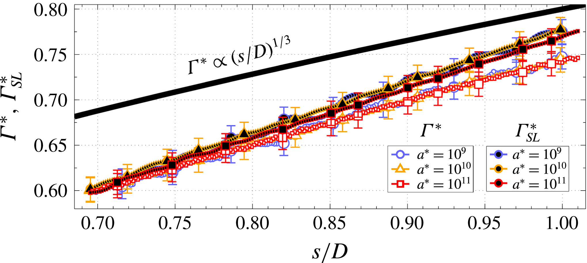
The circulation histories are plotted in figure 6. Both
 $\unicode[STIX]{x1D6E4}^{\ast }$
and
 $\unicode[STIX]{x1D6E4}_{SL}^{\ast }$
respectively collapse for all acceleration cases. The collapse in
 $\unicode[STIX]{x1D6E4}_{SL}^{\ast }$
demonstrates that the feeding rate of normalized circulation is unaffected by increasing the shear layer’s acceleration. Furthermore, the collapse in
 $\unicode[STIX]{x1D6E4}^{\ast }$
demonstrates that in spite of increasing
 $a^{\ast }$
, the same amount of non-dimensional circulation in the starting vortex remains within the azimuthal plane. The collapse may suggest that increasing
 $a^{\ast }$
does not promote significant vortex tilting, and that the shear layer remains bulk two-dimensional in spite of the increase in the instantaneous Reynolds number. However, this can only be speculated from the results. Finally,
 $\unicode[STIX]{x1D6E4}^{\ast }$
is well described by a curve with the shape
 $(s/D)^{1/3}$
, which indicates that in spite of the increase in Reynolds number between the three cases, the circulation is predicted well by inviscid theory presented in Xu & Nitsche (Reference Xu and Nitsche2015).
Starting-vortex circulation
 $(\unicode[STIX]{x1D6E4}^{\ast })$
and shear-layer circulation
 $(\unicode[STIX]{x1D6E4}_{SL}^{\ast })$
for all acceleration cases. Large markers indicate instances of KH shedding. Error bars represent the propagation of 3 % error in the velocity measurements. The solid black line represents a curve with the shape
 $(s/D)^{1/3}$
, which is
 $\unicode[STIX]{x1D6E4}^{\ast }$
as predicted by inviscid theory (Xu & Nitsche Reference Xu and Nitsche2015). The collapse of
 $\unicode[STIX]{x1D6E4}_{SL}^{\ast }$
demonstrates that the circulation feeding rate is unaffected by the shear layer’s acceleration. The collapse in
 $\unicode[STIX]{x1D6E4}^{\ast }$
demonstrates that the same amount of non-dimensional, azimuthal circulation remains within the starting vortex in spite of increases to
 $a^{\ast }$
, and thereby in spite of increases to the instantaneous
 $Re_{\unicode[STIX]{x1D6E4}}$
.

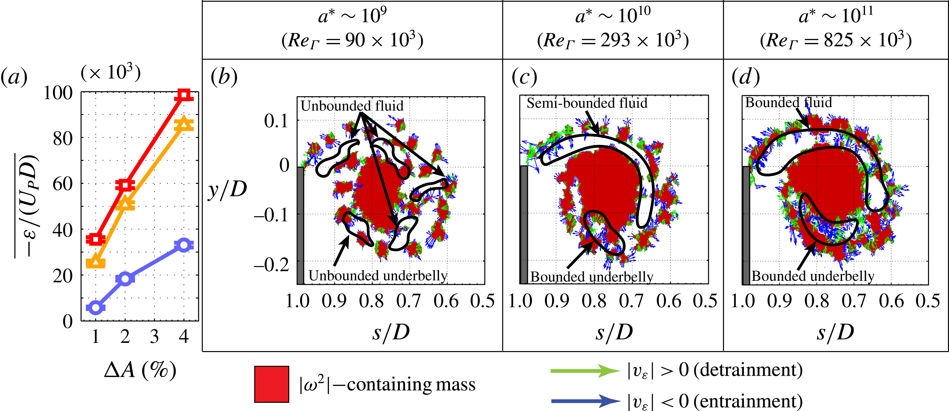
Although the flow topology appears more disorganized at lower accelerations, the entrainment rate does in fact increase with
 $a^{\ast }$
, albeit nonlinearly. Figure 7(a) presents
 $\overline{\unicode[STIX]{x1D700}/(U_{P}D)}$
using various
 $\unicode[STIX]{x0394}A$
thresholds for all three acceleration cases. Although sensitive to the applied threshold, the low-acceleration case consistently exhibits a
 $\overline{\unicode[STIX]{x1D700}/(U_{P}D)}$
that is approximately 50 % that of the mid- and high-acceleration cases, which are nearly identical. This increase in entrainment from the low-acceleration case to the mid- and high-acceleration cases may be elucidated in the topological differences of their respective LHVIs, which are respectively shown for a single run in figure 7 using a
 $\unicode[STIX]{x0394}A$
of 2 %. For the mid- and high-acceleration cases, the small spacing between instabilities results in the formation of a narrow channel between the shear layer and vortex core that binds irrotational fluid and facilitates its roll-up into the starting vortex. Here, irrotational fluid that is located between the shear layer and vortex core rolls up and is inevitably entrained. This is made apparent by the high concentration of entrainment that occurs at the underbelly for both the mid- and high-acceleration cases. In contrast, the large spacing between instabilities for the low-acceleration case reduces the effectiveness of this roll-up, as irrotational fluid is left unbounded along the periphery of the vortex core. As mentioned in the Introduction, this roll-up mechanism has been shown to be crucial in the entrainment of irrotational fluid in vortex rings (Olcay & Krueger Reference Olcay and Krueger2008, Reference Olcay and Krueger2010). The reduced effectiveness of this roll-up in the low-acceleration case may act to decrease the entrainment into the vortex core. The reader is referred to supplementary movie 3, which presents the full sequences for the cases presented in figure 7. It is noted that the observations made here hold true up until a threshold of
 $\unicode[STIX]{x0394}A$
of 6 %, beyond which the shear layer becomes indistinguishable from the vortex core. It is noted that the entrainment observed here must involve turbulent diffusion. As such, the mechanism for exchanging vorticity must be significantly different to that of laminar vortex rings, where vorticity may only be exchanged via laminar diffusion.
(a) Presents
 $\overline{\unicode[STIX]{x1D700}/(U_{P}D)}$
for all three acceleration cases at thresholds of
 $\unicode[STIX]{x0394}A=1\,\%$
, 2 % and 4 %. The error bars represent the standard error of the averages.
 $\overline{\unicode[STIX]{x1D700}/(U_{P}D)}$
is consistently approximately 50 % smaller for the low-acceleration case in comparison to the other two cases. (b–d) Present
 $|\unicode[STIX]{x1D714}^{2}|$
-containing mass regions (red) identified using
 $\unicode[STIX]{x0394}A=2\,\%$
, as well as regions of entrainment and detrainment for the low-, mid- and high-acceleration cases, respectively.
 $a^{\ast }$
, as well as corresponding instantaneous
 $Re_{\unicode[STIX]{x1D6E4}}$
are indicated above the mass-containing fields. For the mid- and high-acceleration cases, the decreased spacing between instabilities produces a channel that rolls-up irrotational fluid. Entrainment is promoted within the channel, and at an ‘underbelly’ of high entrainment located at the channel’s end. This is not observed in low-acceleration case. See supplementary movie 3 for full sequences of the above cases.

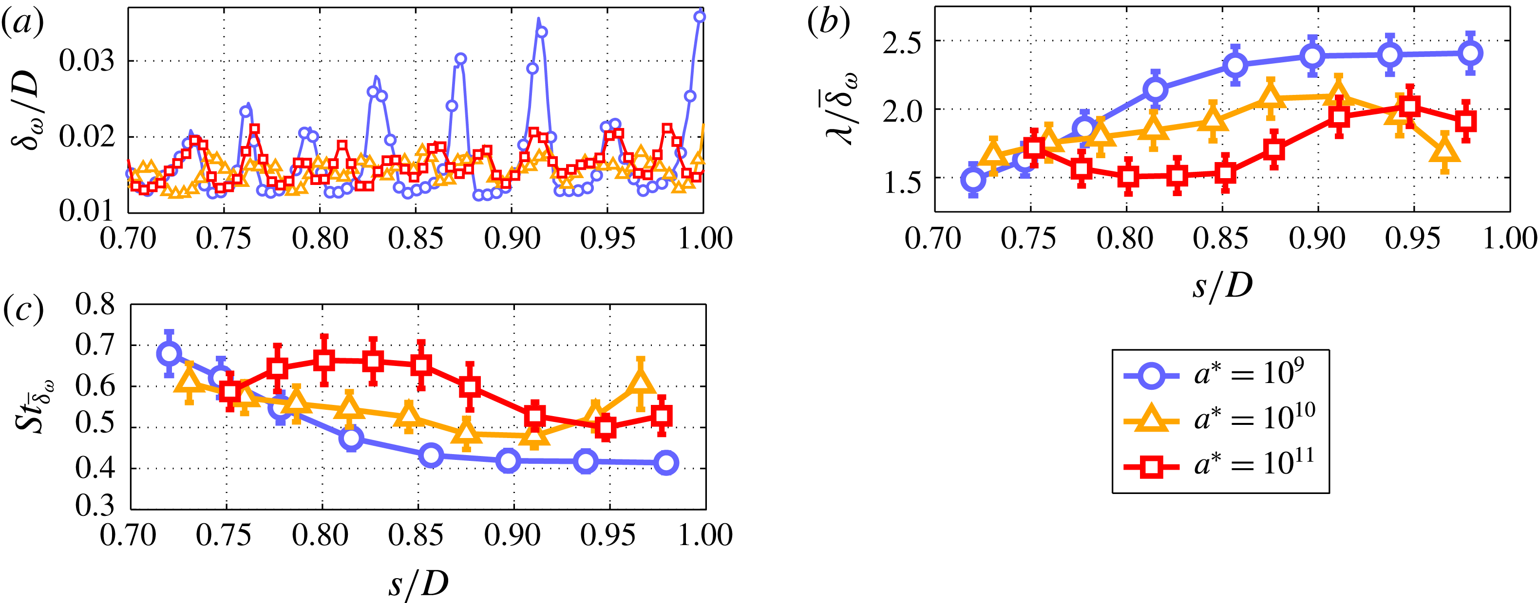
The decrease in spacing between KH instabilities that is qualitatively apparent in figures 5 and 7 is quantified in figure 8(a–c), which respectively present
 $\unicode[STIX]{x1D6FF}_{\unicode[STIX]{x1D714}}/D$
,
 $\unicode[STIX]{x1D706}/\overline{\unicode[STIX]{x1D6FF}}_{\unicode[STIX]{x1D714}}$
and
 $St_{\overline{\unicode[STIX]{x1D6FF}}_{\unicode[STIX]{x1D714}}}$
for the phase averages of all acceleration cases. Figure 8(a) demonstrates that the shear-layer thickness is unaffected by
 $a^{\ast }$
, as all three cases exhibit a mean shear-layer thickness of
 ${\sim}0.15\unicode[STIX]{x1D6FF}_{\unicode[STIX]{x1D714}}/D$
. The periodicity of
 $\unicode[STIX]{x1D6FF}_{\unicode[STIX]{x1D714}}/D$
in all acceleration cases is caused by the shedding of KH instabilities at the plate edge. In fact, the troughs along each plot coincide with the shedding of an instability observed within the
 $|\unicode[STIX]{x1D714}^{2}|$
sequences. Figure 8(b,c) indicates a decrease in shedding wavelength
 $(\unicode[STIX]{x1D706}/\overline{\unicode[STIX]{x1D6FF}}_{\unicode[STIX]{x1D714}})$
, as well as a corresponding increase in Strouhal number
 $(St_{\overline{\unicode[STIX]{x1D6FF}}_{\unicode[STIX]{x1D714}}})$
with increasing
 $a^{\ast }$
. Furthermore, the Strouhal numbers of the non-stationary shear layers presented here are much larger than that for stationary shear layers. Specifically, the shear-layer Strouhal numbers presented here range between 0.4 and 0.7 and are therefore larger than
 $St_{\overline{\unicode[STIX]{x1D6FF}}_{\unicode[STIX]{x1D714}}}=0.13$
, as predicted by linear stability theory for stationary shear layers (Ho & Huerre Reference Ho and Huerre1984). The results demonstrate that the frequency of shedding increases with
 $a^{\ast }$
, and consequently the spacing of instabilities measurably decreases with
 $a^{\ast }$
. Thus, although acceleration has no effect on the transport of vorticity into the starting vortex, as demonstrated by the collapse in circulation shown in figure 6, it does in fact have a significant effect on the topology of the shear layer by decreasing the spacing between instabilities, as demonstrated here. Providing a physical explanation as to why acceleration acts to decrease instability spacing would require extending previous stability theory analyses to account for acceleration. Unfortunately, this is not a trivial endeavour and would require large modifications to the work presented in aforementioned studies. As such, it is not attempted here and left for future studies.
(a) Shear-layer thickness
 $(\unicode[STIX]{x1D6FF}_{\unicode[STIX]{x1D714}}/D)$
against
 $s/D$
for all acceleration cases. The peaks concur with instances of KH shedding determined from
 $|\unicode[STIX]{x1D714}^{2}|$
-field sequences. (b) Shedding wavelength
 $(\unicode[STIX]{x1D706}/\overline{\unicode[STIX]{x1D6FF}}_{\unicode[STIX]{x1D714}})$
and (c) Strouhal number
 $(St_{\overline{\unicode[STIX]{x1D6FF}}_{\unicode[STIX]{x1D714}}})$
against
 $s/D$
, both demonstrating that shedding frequency increases, and consequentially instability spacing decreases with increasing
 $a^{\ast }$
. Error bars in (b, c) represent the propagation of
 $\pm 1~\text{frame}$
in the identification of shedding instances.

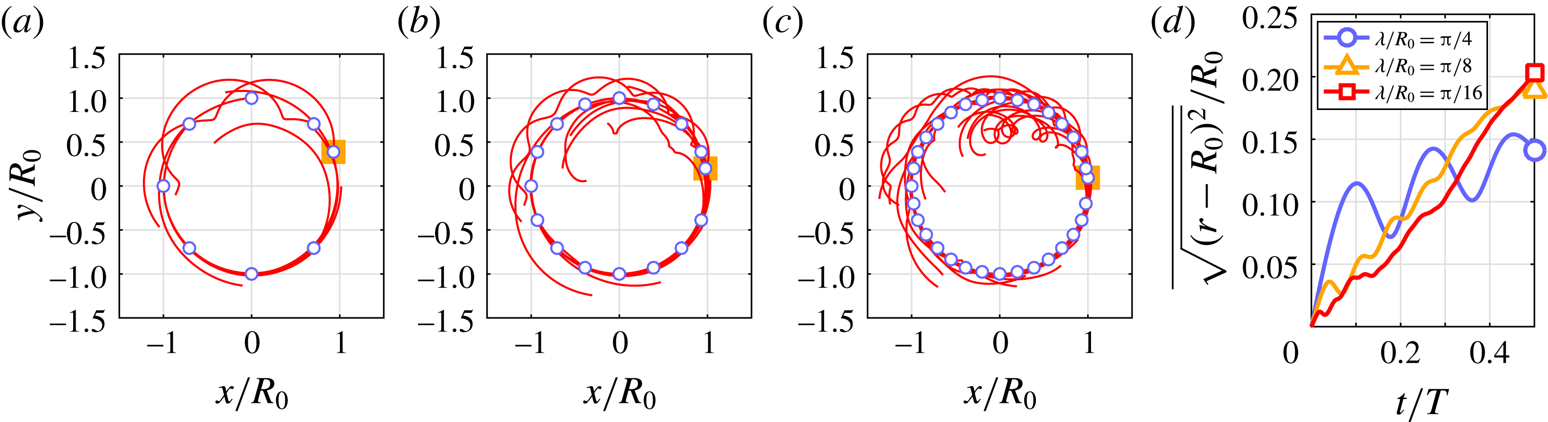
The organization and stability of the shear layer that is observed at larger
 $a^{\ast }$
can be related to the decreased spacing between instabilities. To demonstrate this, three different point-vortex simulations are presented in figure 9, which show that as the wavelength between instabilities decreases within a KH train, then the instabilities will be less prone to deviate from their equilibrium positions if one instability perturbs from its own equilibrium position. To calculate the paths of point vortices, an algorithm developed after Ashbee, Esler & McDonald (Reference Ashbee, Esler and McDonald2013) is used in the current study. The algorithm calculates the paths of
 $N$
point vortices of circulation
 $\unicode[STIX]{x1D6E4}_{i}$
 $(i=1,2,\ldots ,N)$
based on the velocity field that the vortices induce. The motion of point vortices contained within a two-dimensional, simply connected domain is defined as:
 $$\begin{eqnarray}\unicode[STIX]{x1D6E4}_{i}{\dot{x}}_{i}=\frac{\unicode[STIX]{x2202}H}{\unicode[STIX]{x2202}y_{i}},\quad \unicode[STIX]{x1D6E4}_{i}{\dot{y}}_{i}=\frac{\unicode[STIX]{x2202}H}{\unicode[STIX]{x2202}x_{i}}.\end{eqnarray}$$
Here
 $H$
is the Hamiltonian, which can be written as:
 $$\begin{eqnarray}H(\boldsymbol{r}_{1},\ldots ,\boldsymbol{r}_{N})=\mathop{\sum }_{i=1}^{N}\mathop{\sum }_{j=1}^{N}\unicode[STIX]{x1D6E4}_{i}\unicode[STIX]{x1D6E4}_{j}G(\boldsymbol{r}_{i}\boldsymbol{r}_{j})-\frac{1}{2}\mathop{\sum }_{i=1}^{N}\unicode[STIX]{x1D6E4}_{i}^{2}g(\boldsymbol{r}_{i},\boldsymbol{r}_{i}),\end{eqnarray}$$
where
 $G$
and
 $g$
are the Green function and the residual Green function respectively, and
 $\boldsymbol{r}=[x,y]^{\text{T}}$
represents the vector position of a point vortex. The dot accent indicates differentiation with time. For further details regarding the algorithm, the reader is referred to Ashbee et al. (Reference Ashbee, Esler and McDonald2013). In each simulation, a constant value of circulation is divided amongst a system of point vortices that are positioned at equal arclengths along a circle of radius
 $R_{0}$
. If left unperturbed, the vortices would rotate about the circle after a period of
 $T$
. However, to simulate a dimensionlessly equal perturbation of an instability within each vortex system, the vortex positioned at
 $\unicode[STIX]{x1D703}=0$
is shifted by
 $0.5\unicode[STIX]{x1D706}/R_{0}$
counterclockwise along the circle at time
 $t/T=0$
, which causes the vortices to deviate from their circular path.
Figure 9(a–c) presents vortex trajectories for
 $0\leqslant t/T\leqslant 0.5$
for simulations where the inter-vortex arclength is
 $\unicode[STIX]{x1D706}/R_{0}=\unicode[STIX]{x03C0}/4$
,
 $\unicode[STIX]{x03C0}/8$
, and
 $\unicode[STIX]{x03C0}/16$
, respectively. The vortices in (a) deviate greatly from the original circle and follow oscillatory paths due to the perturbation, as indicated by their winding trajectories. This deviation and oscillation becomes increasingly subdued and localized with decreasing arclength, as demonstrated by the organized paths followed by the majority of vortices in (b) and (c). The mean deviation of the vortices is quantified in figure 9(d), which presents the average of
 $\sqrt{(r^{2}-R_{0}^{2})}/R_{0}$
for all three simulations. Here,
 $r$
represents the radial distance of a point vortex from the centre of the circle. The mean deviation of the vortices within the
 $\unicode[STIX]{x1D706}/4$
simulation is widely oscillatory during the entire half-period, and quickly overtakes the mean deviation of vortices within the
 $\unicode[STIX]{x1D706}/8$
and
 $\unicode[STIX]{x1D706}/16$
simulations. The mean deviations of vortices for the
 $\unicode[STIX]{x1D706}/8$
and
 $\unicode[STIX]{x1D706}/16$
simulations do in fact overtake that of the
 $\unicode[STIX]{x1D706}/4$
simulation after
 $t/T>0.4$
. However, the mean deviation of vortices within these simulations is consistently non-periodic. The results demonstrate that decreasing the spacing between instabilities has a stabilizing effect on a shear layer. Specifically, if an individual instability is perturbed, the remaining instabilities are less prone to the deviate from their original path. This provides an analogous explanation as to why shear layers of larger
 $a^{\ast }$
tend to be more organized: perturbations of individual instabilities within shear layers of large
 $a^{\ast }$
have less effect on the overall organization of the KH train.
Point-vortex simulations demonstrating how decreasing
 $\unicode[STIX]{x1D706}/\overline{\unicode[STIX]{x1D6FF}}_{\unicode[STIX]{x1D714}}$
stabilizes a vortex train. Vortices (circles) are positioned along a circle of radius
 $R_{0}$
at dimensionless arclengths of (a)
 $\unicode[STIX]{x03C0}/4$
, (b)
 $\unicode[STIX]{x03C0}/8$
and (c)
 $\unicode[STIX]{x03C0}/16$
, but the
 $\unicode[STIX]{x1D703}=0$
vortex (orange square) is initially perturbed by
 $0.5\unicode[STIX]{x1D706}/R_{0}$
. Vortex trajectories for half a period (
 $T/2$
) are presented in (a–c). (d) Plots the mean deviation of vortices from the circle against
 $t/T$
.

4 Conclusions
To investigate how non-stationarity affects shear-layer entrainment and topology, dye visualizations and time-resolved PIV measurements on a continuously accelerating circular plate were performed in an optical towing tank. Contrary to initial expectations, dye visualizations and
 $|\unicode[STIX]{x1D714}^{2}|$
fields demonstrated that acceleration acts to organize the shear-layer topology. Specifically, KH instabilities abide more closely to a circular path, exhibit consistent spacing, and are less prone to ‘leapfrogging’ as acceleration is increased. Furthermore, in spite of increasing acceleration over three orders of magnitude, the histories of non-dimensional circulation fed through the shear layer, as well as the histories of non-dimensional circulation within the starting vortex collapsed onto a single curve. The collapse in shear-layer circulation demonstrates that the circulation feeding rate is insensitive to the non-stationarity of the shear layer. Also, the collapse in starting-vortex circulation demonstrates that the amount of non-dimensional, azimuthal circulation within the starting vortex remains unchanged in spite of the increase in the shear layer’s instantaneous Reynolds number.
In comparison to stationary shear layers, the instabilities of the non-stationary shear layers studied here exhibit leapfrogging and merging of instabilities. Furthermore, a nonlinear increase in the shedding frequency of instabilities is observed with increasing acceleration, which acts to organize the shear layer by reducing instability leapfrogging and merging. Despite the organizing effect that increasing
 $a^{\ast }$
had on shear-layer topology, the mean entrainment rate along the LHVI was shown to increase with
 $a^{\ast }$
, albeit nonlinearly. This higher entrainment rate for larger
 $a^{\ast }$
was attributed to the closer spacing of instabilities that promotes the roll-up of irrotational fluid between the vortex core and shear layer, which would ultimately be entrained within a coherent ‘underbelly’ near the plate’s centre. This observed decrease in instability spacing was quantified using the Strouhal number and shedding wavelength, both of which indicated a decrease in spacing with increasing
 $a^{\ast }$
. Finally, point-vortex simulations showed that if an individual instability is perturbed from equilibrium, then the remaining instabilities within a KH train are less prone to move off their circular path as the spacing between instabilities decreases. The point-vortex simulations analogously demonstrate how increasing
 $a^{\ast }$
acts to organize the shear layer: as
 $a^{\ast }$
increases, the spacing between instabilities reduces, which in turn reduces the effect of perturbed instabilities on the rest of the KH-instability train. The result provides a simple yet powerful explanation as to why increasing acceleration acts to organize the shear-layer topology. In spite of this, a physical argument as to why instability spacing decreases with increasing acceleration remains to be developed. Developing such an argument would require the modification of previous stability analyses summarized by Ho & Huerre (Reference Ho and Huerre1984), but is left for future studies.
Supplementary movies
Supplementary movies are available at https://doi.org/10.1017/jfm.2016.716.