1. INTRODUCTION
Satellite navigation systems such as the Global Positioning System (GPS) and other Global Navigation Satellite Systems (GNSS), consists of three major segments. These are the Space Segment (SS), a Control Segment (CS), and a User Segment (US) (Parkinson et al., Reference Parkinson, Stansell, Beard and Gromov1995). The GPS satellites in the SS provide navigation messages to users in all weather conditions and receive navigation updates from the ground monitoring stations. The navigation updates are used to synchronize the atomic clocks on board the satellites and to adjust the ephemeris of each satellite's internal orbit model (Dierendock et al., Reference Dierendock, Rusell, Kopitzke and Birnbaum1978). This procedure requires on-going interaction between the CS and the SS to provide the navigation updates to the satellites. If the ground stations become inoperative, the navigation updates cannot be uploaded to the satellites. Therefore, the navigation system as a navigational aid becomes invalid. In order to improve accuracy and survivability of the navigation function for six months without ground contact, the concept of autonomous navigation was introduced (Ananda et al., Reference Ananda, Bernstein, Bruce, Cunningham, Feess, Jorgensen, Menn and Price1984; Codik, Reference Codik1985; Menn, Reference Menn1986; Ananda et al., Reference Ananda, Bernstein, Cunningham, Feess and Stroud1990).
The principle of the autonomous navigation technique is to establish inter-satellite links in the constellation for pseudo-range observations and communications between satellites, and then calculate the positions and the velocities of the satellites in the constellation using the on board estimators (Ananda et al., Reference Ananda, Bernstein, Cunningham, Feess and Stroud1990; Gill, Reference Gill1999). However, observability issues arise for both ephemeris and clocks since the pseudo-range describes only the relative distance between two satellites (Menn and Bernstein, Reference Menn and Bernstein1994). Without periodic corrections from the ground, the constellation's ensemble clock drifts away from the Coordinated Universal Time reference and the ephemeris drifts away from UT1. That is, there is a rotation that leaves the origin fixed, and takes the positions and velocities of one constellation into those of the other. These two constellations cannot be distinguished one from the other by the pseudo-range observations alone.
Unobservable rotation errors need to be addressed. The current autonomous navigation concept uses a distributed Kalman filter with an ephemeris and clock filter in each satellite (Menn and Bernstein, Reference Menn and Bernstein1994). To reduce the rotation error, a three-dimensional constellation rotational constraint algorithm is used. This constraint estimates the rotational component in the range residual and compensates for it. But ground stations are still needed to upload the reference message and monitor the satellites. The Master Control Stations use the ground observations to correct the slow rotational effect that is not well observed by the on board estimation, and upload the reference trajectories and clock corrections to the satellites every 210 days (Bernstein et al., Reference Bernstein, Bowden and Gartside1993).
A concept of “anchoring” was introduced to enhance and improve the performance of the navigation system. The anchor concept interjects a virtual satellite, which is located on a known (surveyed) position on earth into the GPS system. This anchor provides a rigid reference to the GPS constellation and makes the residual constellation rotation with respect to earth observable and correctable (Rajan et al., Reference Rajan, Brodie and Rawicz2003).
By introducing the observations of the baseline's orientation between two satellites into the navigation system, the rotation of the constellation mentioned above can also be obtained (Chen et al., Reference Chen, You and Jiao2005; Kai et al., Reference Kai, Chunling and Liangdong2008). However, due to the rapid movement of the satellites, the orientation of the baseline between two satellites changes rapidly. Therefore, it is very difficult to measure the orientation of a baseline.
In this paper, a differential measurement method to measure the rotation of the constellation by observing variable celestial sources is proposed for the first time. As mentioned before, the rotation of the constellation as a whole cannot be distinguished by using the inter-satellite pseudo-range observations alone. After using a Kalman filter and a three-dimensional constellation rotational constraint algorithm, a residual constellation rotation still exits (Menn, Reference Menn1986; Menn and Bernstein, Reference Menn and Bernstein1994; Ananda et al., Reference Ananda, Bernstein, Cunningham, Feess and Stroud1990). We use one satellite in conjunction with the other to observe celestial sources, as Very Long Baseline Interferometry (VLBI) does, to determine the positions of the celestial sources. Since the observation results include the effect of the constellation rotation residual, the residual constellation rotation can be obtained by comparing the observation positions with the theoretical positions of the celestial sources.
This paper is organised as follows. In Section 2, the differential measurement method is proposed. The simulation results and efficiency analysis of the proposed method are presented in Section 3. Section 4 is the discussion and conclusion.
2. THE DIFFERENTIAL MEASUREMENT METHOD
The differential measurement method uses one satellite in conjunction with another to observe celestial sources to determine the positions of the celestial sources. The constellation rotation angle is treated as a global variable. Since the observation results include the effect of the constellation rotation, the constellation rotation angle can be obtained by comparing the observation positions with the theoretical positions of the celestial sources.
2.1. The rotation of the satellite constellation
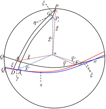
The satellite ephemeris is given in an Earth-Centred-Earth-Fixed (ECEF, hereafter E) coordinate system whose orientation at any time will depend on the Earth rotation (Dierendock et al., Reference Dierendock, Rusell, Kopitzke and Birnbaum1978). The orbit of the satellite is described by six Keplerian elements, which are i (inclination), ϖ (argument of perigee), Ω (right ascension of the ascending node), a (semi-major axis), e (eccentricity) and M 0 (mean anomaly). Let θ be a small rotation. Rotation of the constellation as a whole by θ changes the Keplerian message parameters i, Ω and ϖ with a, e, M 0 being invariant under rotation. In fact, due to the rotation of the constellation, the orbit is given in a coordinate system that has a rotation with respect to E (denoted as E′). The small rotation θ between these two coordinate systems can be described by three angles, these are ξ, η, γ, as shown in Figure 1. Where ξ is the angle between Z axis and Z′ axis in latitude, η is the angle between Z axis and Z′ axis in longitude, and γ is the angle between X axis and X′ axis in longitude.
Rotation angles between two coordinate systems. PG = AD = ξ, GP c = η, DA c = γ, O − XYZ, are the coordinate axises of the coordinate system E. O − X′Y′Z′ are the axes of E′. The black circular arc ( $\widehat{{QE}}$) is the equator of coordinate system E, and the blue circular arc (
 $\widehat{{DH}}$) is the equator of E′. The red circular arc (
 $\widehat{{{A_c}E}}$) is the equator of coordinate system E′ after rotating an angle ξ about the Y axis.

A vector  $\vec r$ can be transformed from coordinate system E to E′ using the rotation matrices. As shown in Figure 1, the mathematical description of the transformation is as follows:
 $$\vec r = {R_3}\left( { - \gamma} \right){R_1}\left( \eta \right){R_2}\left( { - \xi} \right)\vec r^{\,\prime} $$
Where  $\vec r$ is the vector described in coordinate system E,
 $\vec r^{\,\prime} $ is the same vector, but described in E′. R 1(φ), R 2(φ) and R 3(φ) are the transformation matrices that rotate an angle φ about the X, Y and Z axis. The specific form of the rotation matrix can be found in Arfken (Reference Arfken1985).
2.2. Angle difference measurement
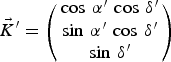
Considering a celestial object at infinite distance, its unit direction vector in E can be written as:
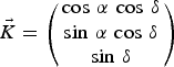 $$\vec K = \left( {\matrix{ {\cos \,\alpha \,\cos \,\delta} \cr {\sin \,\alpha \,\cos \,\delta} \cr {\sin \,\delta} \cr}} \right)$$
Where α and δ are the right ascension and declination respectively. When the satellites observe the celestial object, the observation result can be written in E′ as follows:
 $$\vec K^{\prime} = \left( {\matrix{ {\cos \,\alpha ^{\prime} \,\cos \,\delta ^{\prime} } \cr {\sin \,\alpha ^{\prime} \,\cos \,\delta ^{\prime} } \cr {\sin \,\delta ^{\prime} } \cr}} \right)$$
In Equation (3), α′ and δ′ can be approximated as  $\alpha ^{\prime} = \alpha + \Delta \alpha ^{\prime} $ and
 $\delta ^{\prime} = \delta + \Delta \delta ^{\prime}$. Combining Equations (2) and (3), we get Equation (4):
 $$\delta \vec K = \vec K^{\prime} - \vec K = \left( {\matrix{ { - \sin \,\alpha \,\cos \,\delta \,\Delta \alpha ^{\prime} - \cos \,\alpha \,\sin \,\delta \,\Delta \delta ^{\prime} } \cr {\cos \,\alpha \,\cos \,\delta \,\Delta \alpha ^{\prime} - \sin \,\alpha \,\sin \,\delta \,\Delta \delta ^{\prime} } \cr {\cos \,\delta \,\Delta \delta ^{\prime} } \cr}} \right)$$
Taking Equation (1) into account, the relation between  $\vec K$ and
 $\vec K^{\prime} $ can be written approximately as follows:
 $$\vec K = {R_3}\left( { - \gamma} \right){R_1}\left( \eta \right){R_2}\left( { - \xi} \right)\vec K^{\prime} = \left( {\matrix{ 1 & { - \gamma} & \xi \cr \gamma & 1 & \eta \cr { - \xi} & { - \eta} & 1 \cr}} \right)\vec K^{\prime} $$
Substituting Equation (5) into Equation (4), the angle difference between the satellite observation result and the theoretical value can be written as:
 $$\eqalign{& \Delta \alpha ^{\prime} = \left( {\xi \,\sin \,\alpha - \eta \,\cos \,\alpha } \right)\,\tan \,\delta - \gamma \cr & \Delta \delta ^{\prime} = \xi \,\cos \,\alpha + \eta \,\sin \,\alpha } $$
The small rotation angles of the constellation can be obtained by solving Equation (6).
2.3. Time differential measurement
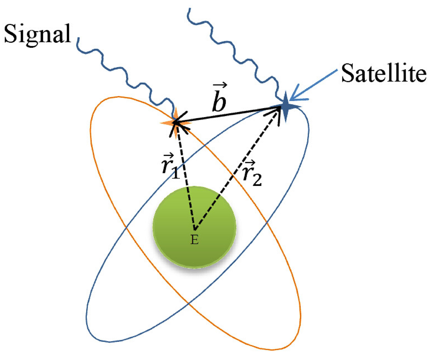
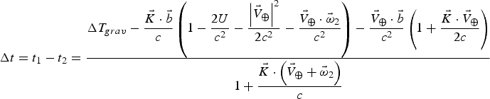
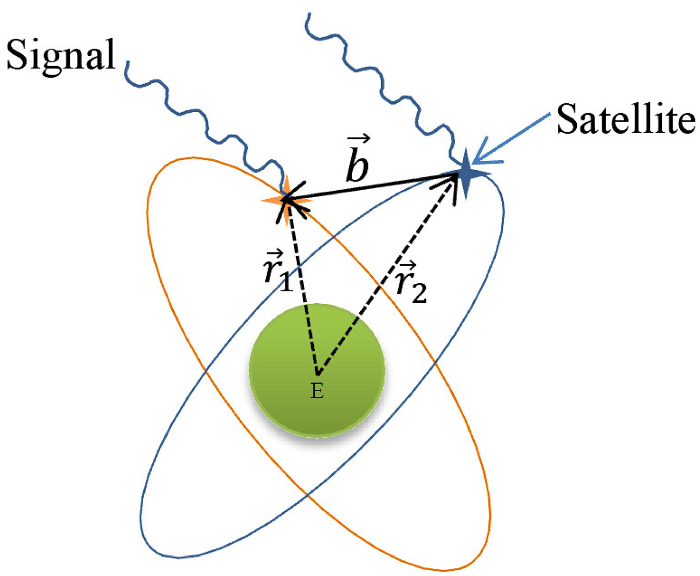
In order to solve Equation (6), we use the differential measurement method to obtain the angle difference between the satellite observation result and the theoretical value Δα′ and Δδ′. As shown in Figure 2, we use one satellite in conjunction with the another to observe celestial sources, as Very Long Baseline Interferometry (VLBI) does, to determine the positions of the celestial sources. Considering two satellites in the constellation in conjunction with each other as a baseline  $\vec b$ to observe a celestial source at infinite distance, the theoretical time delay between these two satellites is given as (Petit and Brian, Reference Petit and Brian2010):
 $$\Delta t = {t_1} - {t_2} = \displaystyle{{\Delta {T_{grav}} - \displaystyle{{\vec K \cdot \vec b} \over c}\left( {1 - \displaystyle{{2U} \over {{c^2}}} - \displaystyle{{{{\left\vert {{{\vec V}_ \oplus}} \right\vert}^2}} \over {2{c^2}}} - \displaystyle{{{{\vec V}_ \oplus} \cdot {{\vec \omega} _2}} \over {{c^2}}}} \right) - \displaystyle{{{{\vec V}_ \oplus} \cdot \vec b} \over {{c^2}}}\left( {1 + \displaystyle{{\vec K \cdot {{\vec V}_ \oplus}} \over {2c}}} \right)} \over {1 + \displaystyle{{\vec K \cdot \left( {{{\vec V}_ \oplus} + {{\vec \omega} _2}} \right)} \over c}}}$$
Where  $\vec b = {\vec r_1} - {\vec r_2}$,
 ${\vec r_i}$ is the position of the ith satellite,
 ${\vec V_ \oplus} $ is the barycentric velocity of Earth, U is the gravitational potential at the geocentric neglecting the effects of the Earth's mass, and
 ${\vec \omega _2}$ is the geocentric velocity of the second receiver at t 2, ΔT grav is the differential gravitational time delay and c is the velocity of light in a vacuum.
Two satellites in conjunction with each other as a baseline to observe celestial objects.
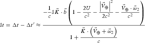
The observation equation can be written as:
 $$\delta t = \Delta t - \Delta t^{\prime} \approx \displaystyle{{ - \displaystyle{1 \over c}\delta \vec K \cdot \vec b\left( {1 - \displaystyle{{2U} \over {{c^2}}} - \displaystyle{{{{\left\vert {{{\vec V}_ \oplus}} \right\vert}^2}} \over {2{c^2}}} - \displaystyle{{{{\vec V}_ \oplus} \cdot {{\vec \omega} _2}} \over {{c^2}}}} \right)} \over {1 + \displaystyle{{\vec K \cdot \left( {{{\vec V}_ \oplus} + {{\vec \omega} _2}} \right)} \over c}}}$$
Where Δt is the theoretical time delay calculated by Equation (7), and Δt′ is the observation value. Substituting Equation (4) into Equation (8), Δα′ and Δδ′ can be obtained using multiple time delay observations. Substituting the results into Equation (6), the three rotation angles can be obtained.
To get the time delay between the two satellites in question, one possible way is to observe the periodic celestial sources, such as X-ray pulsars. A pulsar is a highly magnetized, rotating neutron star that emits a beam of electromagnetic radiation. Neutron stars are very dense, and have short, regular rotational periods. This produces a very precise interval between pulses that range from roughly milliseconds to seconds for an individual pulsar. By observing the time of a pulsar's arrival (TOA) at different satellites, as shown in Figure 2, the time delay between two satellites can be given as:
 $$\Delta t = {t_1} - {t_2} + \Delta {t_{grav}} + \Delta {t_{clock}} + \Delta {t_{other}}$$
Where t i is the X-ray pulsar's TOA measured by the ith satellite, Δt grav is the differential gravitational time delay, Δt clock is the clock error, and Δt other is the other effects, such as the instrument error.
3. EFFICIENCY ANALYSIS AND SIMULATION RESULTS
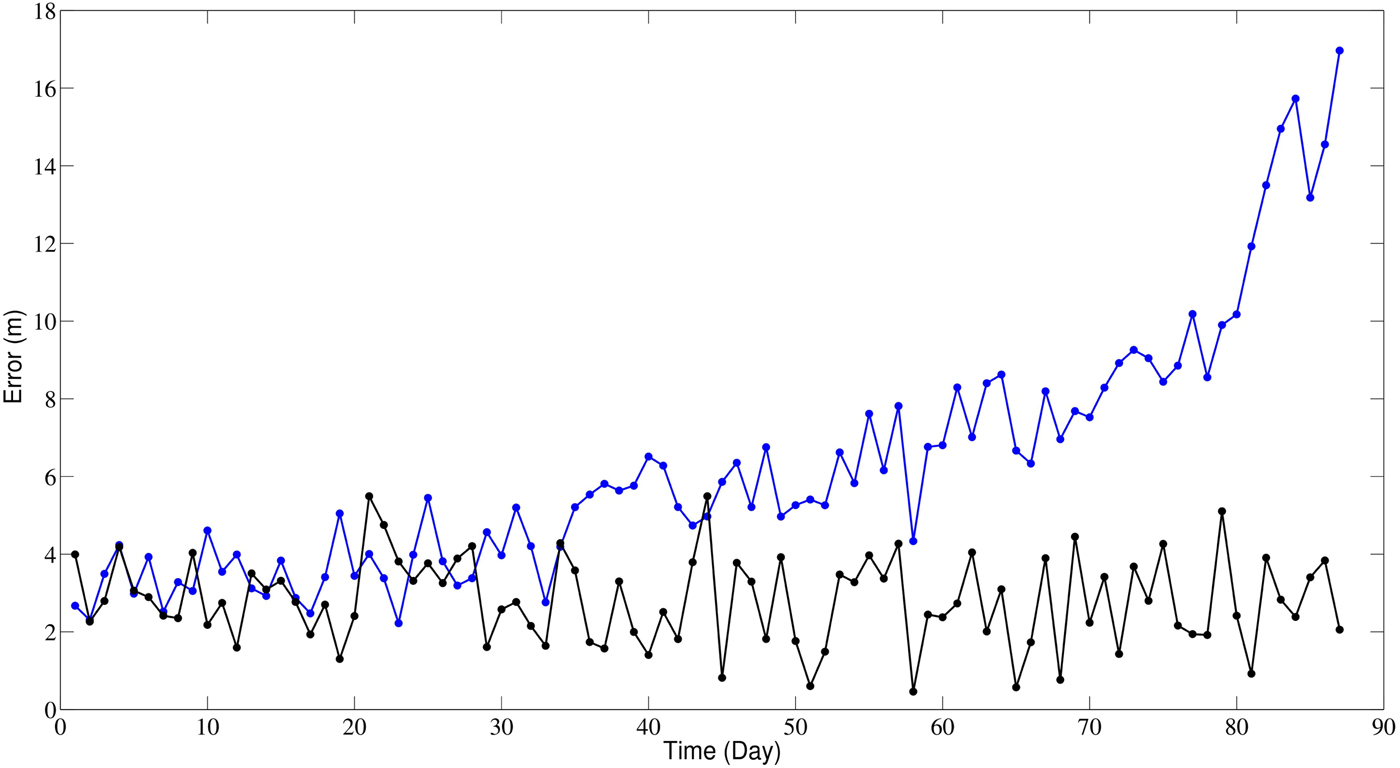
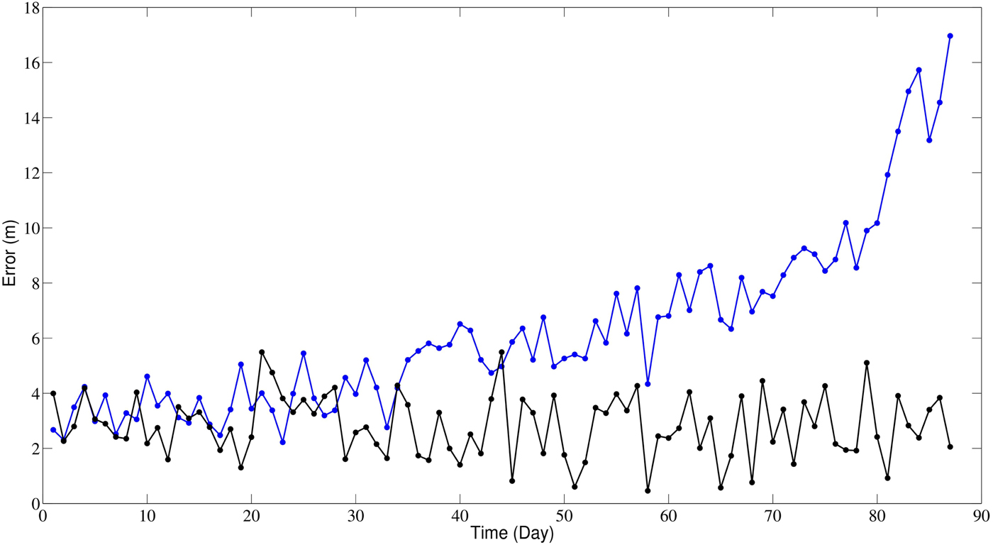
In order to verify the feasibility of the proposed method, we show the simulation results in this section. We use the GPS satellites as experimental subjects. The GPS satellites’ orbits are simulated with the Satellite Tool Kit (STK). A 27/3 (27 satellites in 3 orbits) constellation with the satellites in a plane at equal speed and the satellites of one plane to an adjacent one staggered by 1/3 in orbital angle is used for simulation. The crosslink is a point-to-point high performance crosslink with ranging measurement capability of 0·05 m (0·167 ns) rms. Range measurements were made every 15 minutes to four neighbouring satellites. The satellites' orbit for 90 days are predicted and a residual constellation rotation with an angular speed of 1·8 mas/day is assumed. The X-ray pulsar's TOA measurement accuracy on board is set to 10 ns. We use Equation (8) to solve the angle difference Δα′ and Δδ′, then substitute the results into Equation (6) to get the rotation angles. Then we use the measurement rotation angles to eliminate the rotation effect, and compare the satellites’ positions with those without rotation. As shown in Figure 3, the satellites’ position error can be reduced from 18·0 m to 4·0 m using this differential measurement method.
The feasibility of the proposed method. The blue line is the satellites’ position root mean square error with the rotation effect. The black line (bottom line) is the satellites’ position root mean square error after using the differential measurement method to eliminate the rotation effect.
4. CONCLUSIONS
In this paper, a differential measurement method for aiding autonomous navigation of satellites in constellation using periodic celestial sources is proposed. Using the signal from variable X-ray sources could potentially provide high accuracy TOA measurements between vehicles. Compared to the methods mentioned in the introduction (which are Kalman filter method and anchor concept), the advantages of the differential measurement method are as follows: 1) The navigation system can operate without ground stations sending data to each satellite, which results in significant reduction in operational cost; 2) Pulsar-based time-scale has a precision comparable to the uncertainties in International Atomic Time-scales (TAI) (Hobbs et al., Reference Hobbs, Coles, Manchester, Keith, Shannon, Chen, Bailes, Bhat, Burke-Spolaor, Champion, Chaudhary, Hotan, Khoo, Kocz, Levin, Oslowski, Preisig, Ravi, Reynolds, Sarkissian, Straten, Verbiest, Yardley and You2012). By observing X-ray pulsars, one could set up such a time-scale, and the constellation's ensemble clock's drifting away from the Coordinated Universal Time reference can be prevented.
However, the X-ray pulsar's TOA accuracy is about 100 ns by observing 103 s, corresponding to a 30 m accuracy (Emadzadeh and Speyer, Reference Emadzadeh and Speyer2011; Sheikh, Reference Sheikh2005; Sheikh and Paul, Reference Sheikh and Paul2007), which is not good enough for navigation nowadays. Thus, the X-ray pulsar's TOA observation accuracy still needs to be improved. For future navigation systems application, several detector system improvements could be considered to enhance performance. These would include increased detector area, improved quantum efficiency, lower background rates, and longer observation durations. In addition, several processing enhancements could be used such as optimising the energy band selected to maximise the accuracy, and potentially pre-filtering the data before cross correlation to reduce the white noise at frequencies that are not useful, as Sheikh and Paul (Reference Sheikh and Paul2007) suggest. Further studies are planned to investigate improvements to the TOA analysis techniques, including switching to the frequency domain for the cross correlation process using a method such as that described by Taylor (Reference Taylor1992). Future planned research anticipates that these accuracies will improve using refined techniques and additional sources.
ACKNOWLEDGEMENTS
We gratefully acknowledge the help and discussion with our colleague Dr. Ming Zhao.
FINANCIAL SUPPORT
This work was supported by grants from the National Science Foundation of China (grant number NSFC No. 11273003).