1. INTRODUCTION
As one of the main contributions of the navigation message, the provision of the Global Positioning System (GPS) satellite clock offset should be guaranteed to ensure a navigation service. The broadcast ephemerides are the traditional satellite clock offset service and they are provided for real-time users. The broadcast ephemerides are obtained using the prediction operation and they are broadcast within the navigation message. The precise satellite clock offset is hard to forecast since the rubidium and caesium atomic standards of the GPS satellites are subject to clock noise and frequency variations. The broadcast ephemerides achieve a typical user range offset at the 1·5 metre level (Li et al., Reference Li, Chen, Wang, Hu and Liu2010a). Even though their accuracy is not fully competitive with precise data products, the broadcast ephemerides are well suited for numerous applications, such as visibility analysis, quality control of observation data, or relative navigation. Satellite clock prediction products, which are also provided in the predicted part of the ultra-rapid orbits provided by the International Global Navigation Satellite System Service (IGS) (Dow et al., Reference Dow, Neilan and Rizos2009), will deviate quickly from the true values by several decimetres or even metres. With the development of un-differenced observations-based Precise Point Positioning (PPP) (Zumberge et al., Reference Zumberge, Heflin, Jefferson, Watkins and Webb1997), high-precision satellite clock estimation is used in PPP and is carried out by the IGS as a routine service. Initially, only the “final” satellite clock products were provided by IGS. However, the final precise satellite orbit and clock products required by PPP suffered a latency of about 15 days. The initial satellite clock offset is given at 15 min intervals and is included in IGS sp3 files. Because the interpolation of the 15 min satellite clock offset is possible at the precision level of a few decimetres (Bock et al., Reference Bock, Dach, Jäggi and Beutler2009), the clock files containing separate combinations of satellite/station clocks at 5 min sampling intervals have been available since 26 December 1999 and the clock combinations became the official IGS clock products on 5 November 2000. Five minute clock sampling shows an interpolation of satellite clocks below the decimetre level. To keep clock interpolation offsets at or below the centimetre-level (Bock et al., Reference Bock, Dach, Jäggi and Beutler2009), starting with GPS Week 1410 (14 January 2007), the IGS final clock combinations also include additional clock files at 30 sec sampling. These products contain the satellite clock series. Since 2013, the IGS Real-Time Service (RTS) has been implemented and real-time PPP has become feasible. The real-time clocks are published as Radio Technical Commission for Maritime Services (RTCM) State-Space Representation (SSR) correction streams and broadcast over the internet using the Networked Transport of RTCM via Internet Protocol (NTRIP).
The precise clock offset is usually estimated with the phase and code observations of a global network (Senior et al., Reference Senior, Ray and Beard2008; Hauschild and Montenbruck, Reference Hauschild and Montenbruck2009; Bock et al., Reference Bock, Dach, Jäggi and Beutler2009; Li et al., Reference Li, Chen, Wang, Hu and Liu2010a; Reference Li, Wang, Chen, Hu and Wang2010b; Ge et al., Reference Ge, Chen, Dousa, Gendt and Wickert2012). For this clock estimation, the ionosphere-free phase (L1/L2) and code (P1/P2) observations from different types of receivers are used. In other words, the reference of the current clock products is based on L1/L2 and P1/P2. The first consequence of this estimation scheme is that the satellite clock offset contains the contribution of the satellite hardware delay bias so that satellite clock estimates from different observations, that is, navigation signals (L1 or L2), might differ. In order to meet the requirement of the single-frequency user, the single-frequency clock correction is obtained based on the current satellite clock products and the Differential Code Bias (DCB(P1-P2)). While some receivers track the P1 and P2 observables, other receivers only provide C1 and P2. Therefore, the DCB(C1-P1) should be compensated to improve C1 observation-based precise positioning (Li et al., Reference Li, Xu, Li, Huang and Wang2016a). With the development of Global Navigation Satellite Systems (GNSSs), some systems such as the Chinese BeiDou system (Yang et al., Reference Yang, Li, Xu, Tang, Guo and He2011; Steigenberger et al., Reference Steigenberger, Hugentobler, Hauschild and Montenbruck2013), the modernised GPS satellites, the European Galileo system (Paziewski and Wielgosz, Reference Paziewski and Wielgosz2014) and the Japanese Quasi-Zenith Satellite System (QZSS) (Hauschild et al., Reference Hauschild, Steigenberger and Rodriguez-Solano2012) broadcast navigation signals on three or more carrier frequencies. As a consequence, a new bias is introduced when investigating triple-frequency phase observations. This bias shows that difference exists between the estimated satellite clocks from ionosphere-free code and carrier phase observations using either the L1/L2 and P1/P2 observations or the L1/L5 and P1/P5 observations. This bias is defined as Inter-Frequency Clock Bias (IFCB) (Li et al., Reference Li, Li, Xiao, Wang and Xu2016b). The IFCB reveals that the current clock products computed with L1/L2 and P1/P2 cannot be used directly and the IFCB should be considered carefully for a triple-frequency user in undifferenced data processing. The 24-h IFCB shows that it contains both variable and constant parts and its constant part is called the Inter-Frequency Hardware Bias (IFHB).
Due to the IFCB variable contribution, the general method, which just considers the constant bias, is inapplicable for the triple-frequency GPS satellite clock offset. The GPS triple-frequency satellite clock offset can be obtained based on the current satellite clock products estimated with L1/L2 and P1/P2 observations, the DCB(P1-P2), DCB(P1-P5) and finally the IFCB products. The variation of the IFCB suggests that the IFCB service for triple-frequency GNSS cannot be simplified as the DCB(P1-P2) and DCB(P1-P5) services for which only a daily or weekly constant is provided. The IFCB cannot be replaced by the current DCB(P1-P2) and DCB(P1-P5) products, although it can be expressed as a function of the DCB(P1-P2) and DCB(P1-P5). Thus, the service strategy for the GPS triple-frequency satellite clock offsets is discussed and the performance of the computed clock offset is analysed.
Section 2 introduces the satellite clock offset products and observation references. In this section, some main estimation methods for estimating the current clock offset products and selected observation reference are discussed. Section 3 presents the service strategy for the GPS triple-frequency satellite clock offsets. Section 4 discusses application of the GPS triple-frequency satellite clock offsets. In this same section, the performance of the DCB(P1-P2), DCB(P1-P5) and IFCB, as well as the application of the GPS triple-frequency satellite clock offsets are analysed. Finally, Section 5 summarises the main findings.
2. SATELLITE CLOCK OFFSET PRODUCTS AND OBSERVATION REFERENCE
The estimated satellite clock offsets contain the contribution of the biases in the observations so that there are biases between the estimated clock offsets with different observations (that is, the combination of signals transmitted from the same satellite). Generally, the reference observation (that is, signal) is selected and the corresponding satellite clock offsets are computed. Based on the computed satellite clock offsets and the biases between the reference observation and other observations, the satellite clock offsets of all observations are obtained. For the triple-frequency observation, many observations can be selected as the reference observation. The observation reference of the current GPS satellite clock offset product is based on the L1/L2 and P1/P2 observations:
 $$IF(L_1 ,L_2 )^{r,s} = \rho + \delta^r - \delta^s + const_{1,2} + T + \varepsilon_1$$
 $$IF(P_1 ,P_2 )^{r,s} = \rho + \delta^r + b_{1,2}^r - \delta^s - b_{1,2}^s + T + \omega_1$$
where superscript r and s indicate receiver and tracked satellite; ρ is the satellite-to-receiver range, T is the tropospheric delay; δr and δs are receiver and satellite clock; const 1, 2 is the ambiguity of L1/L2; ε1 is the noise of L1/L2; ω1 is the noise of P1/P2 and b 1,2r and b 1,2s are the receiver and satellite hardware bias of P1/P2. Based on Equations (1) and (2), some methods are used to estimate the current satellite clock offset. In the general processing method (Hauschild and Montenbruck, Reference Hauschild and Montenbruck2009), the satellite clock offsets are normally estimated from a reference network by iterative batch processing. It is necessary to estimate all parameters including the ambiguities, the receiver clocks, the satellite clocks and the tropospheric delay. To improve computational efficiency, the phase-differenced methods are presented (Bock et al., Reference Bock, Dach, Jäggi and Beutler2009; Li et al., Reference Li, Chen, Wang, Hu and Liu2010a; Ge et al., Reference Ge, Chen, Dousa, Gendt and Wickert2012). In this method, the ambiguity parameters are cancelled based on the epoch-differenced algorithm. Independently from the method used to compute the satellite clock, the hardware delay from the receiver is included into the receiver clock, while the hardware delay from the satellite is included into the satellite clock. Thus, the current clock product also contains the contribution of the hardware delay of the satellite. The estimated satellite clock offset is:
 $$\overline {\delta _{1,2}^s } =\delta^s+b_{1,2}^s =\delta ^s+b_1^s +{f_2^2 \over f_1^2 -f_2^2} \hbox{DCB}^{\rm s}(\hbox{P1}-\hbox{P2})=\delta^{s}+b_2^{s} + {f_1^2 \over f_1^2 -f_2^2} \hbox{DCB}^{\rm s}(\hbox{P1}-\hbox{P2})$$
where  $\overline{\delta _{1,2}^{s}}$ is the estimated satellite clock using the L1/L2 and P1/P2 observations; b 1s and b 2s are the satellite hardware delay of P1 and P2; f 1 and f 2 are the frequencies of P1 and P2 and DCBs(P1-P2) is the satellite DCB between P1 and P2. In the single-frequency observation-based positioning (Li et al., Reference Li, Tang, He, Wu, Hu and Chen2013a), the satellite clock offsets of the P1(L1) and P2(L2) observations are computed:
 $$\overline {\delta _1^s} =\delta ^s+b_1^s =\overline {\delta _{1,2}^s} -{f_2^2 \over f_1^2 -f_2^2} \hbox{DCB}^{\rm s}(\hbox{P1}-\hbox{P2})$$
 $$\overline {\delta _2^s } =\delta ^s+b_2^s =\overline {\delta _{1,2}^s} -{f_1^2 \over f_1^2 -f_2^2} \hbox{DCB}^{\rm s}(\hbox{P1}-\hbox{P2})$$
where  $\overline {\delta _{1}^{s}}$ and
 $\overline {\delta _{2}^{s}}$ are the satellite clock offsets of the observations P1(L1) and P2(L2). Equations (3)–(5) indicate that the current satellite clock product fully meets the requirement of the dual-frequency user of combined and un-combined PPP.
To meet the requirement of the triple-frequency combined PPP user, the satellite clock offsets of the ionosphere-free combinations should be computed and provided. Besides Equations (1) and (2), other ionosphere-free carrier and code observations can be written for a triple-frequency user:
 $$IF(L_1 ,L_5 )^{r,s} = \rho +\delta ^r-\delta ^s+const_{1,5} +T+\varepsilon _2$$
 $$IF(P_1 ,P_5 )^{r,s} = \rho +\delta ^r+b_{1,5}^r -\delta ^s-b_{1,5}^s +T+\omega_2$$
In order to compute the triple-frequency satellite clock offset using Equations (1), (2), (6) and (7) based on the general method, the estimated ambiguity and clock parameters double. Such computations appear too time-consuming to be used for estimating the high-rate satellite clock correction in real-time (Li et al., Reference Li, Chen, Wang, Hu and Liu2010a; Reference Li, Wang, Chen, Hu and Wang2010b; Ge et al., Reference Ge, Chen, Dousa, Gendt and Wickert2012). To improve the computational efficiency and simplify the service, a new approach for estimating the satellite clock offset of triple-frequency observations has been presented (Li et al., Reference Li, Li, Xiao, Wang and Xu2016b). This approach shows that the satellite clock offset estimated with L1/L5 and P1/P5 can be recovered by the IFCB and the current clock products computed with L1/L2 and P1/P2, as reference observations. The satellite clock offset of L1/L5 and P1/P5 is:
 $$\overline {\delta _{1,5}^s} = \delta^s + b_{1,5}^s = \overline {\delta_{1,2}^s} + IFCB^s$$
where IFCB s is the satellite IFCB. The key principle of the new approach is included in the IFCB estimation itself. As stated in Montenbruck et al. (Reference Montenbruck, Hugentobler, Dach, Steigenberger and Hauschild2012) and Li et al. (Reference Li, Zhou, Wu and Wang2012; Reference Li, Zhou and Wu2013b; Reference Li, Chen, Wu, Hu, He, Tang, Gong and Chen2013c) for the IFCB estimation, only triple-frequency phase observations are used so that the constant satellite hardware bias is absorbed by the ambiguity and is absent from the estimated IFCB. Therefore, if this IFCB product is used to compute the satellite clock offset for the triple-frequency user, the effect of the estimated clock products on the undifferenced positioning would be noticeable (Li et al., Reference Li, Xu, Li, Huang and Wang2016a). To overcome the limitation of these studies, an improved method for estimating the IFCB is presented in Li et al. (Reference Li, Li, Xiao, Wang and Xu2016b). In this method, the phase observation is used to compute the variable part of the IFCB, while the code observation is used to compute the constant part of IFCB. For IFCB modelling, a combined linear and fourth harmonic function is used (Li et al., Reference Li, Zhou and Wu2013b; Reference Li, Chen, Wu, Hu, He, Tang, Gong and Chen2013c; Reference Li, Li, Xiao, Wang and Xu2016b). This model is written as:
 $$IFCB^{s}\hbox{(}t\hbox{)} = d + e \cdot t + \sum\limits_{i=1}^4 {\lambda _i\, \cdot} \sin \left({2\pi \over T_i} \cdot t + \theta_i \right)(t = 0 - 24h)$$
where d is a constant; e is the coefficient of the linear terms; i is the order of the harmonics; T i is the period; θi is an initial phase offset and λi is the amplitude. All together 14 coefficients are involved in the IFCB models.
In order to realise triple-frequency un-combined PPP, the triple-frequency un-combined satellite clock offset should be estimated. According to Equations (4) and (5), the satellite clock offset of the P1(L1) and P2(L2) observations is obtained. The computed satellite clock offset of the P5(L5) observation can be written as follows:
 $$\overline {\delta _5^s } =\overline {\delta _{1,5}^s } - {f_1^2 \over f_1^2 -f_5^2 }\hbox{DCB}^{\rm s}(\hbox{P1}-\hbox{P5})=\overline {\delta _{1,2}^s } +IFCB - {f_1^2 \over f_1^2 -f_5^2} \hbox{DCB}^{\rm s}(\hbox{P1}-\hbox{P5})$$
Based on the current satellite clock offset products estimated with the reference observation L1/L2 and P1/P2 and the computed IFCB, the triple-frequency un-combined satellite clocks can be computed with Equations (4), (5) and (10) using the DCB (P1-P2) and DCB (P1-P5) products.
3. SERVICE STRATEGY FOR THE GPS TRIPLE-FREQUENCY SATELLITE CLOCK OFFSET
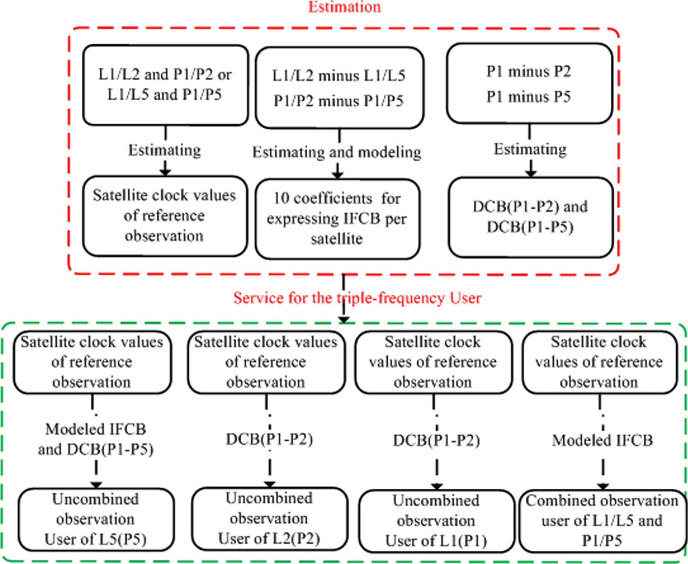
Based on the current estimated satellite clock products of the observation reference (L1/L2 and P1/P2), the DCB(P1-P2), DCB(P1-P5) and IFCB products, the triple-frequency satellite clock offsets are computed. The DCB(P1-P2) and DCB(P1-P5) are estimated as a constant for each day, while the IFCB is computed as a time-variant value. The time-variant IFCB makes the GPS triple-frequency satellite clock offset more difficult to provide as a service. However, it can be seen that the combined linear and fourth order harmonic function can well describe IFCB (Li et al., Reference Li, Li, Xiao, Wang and Xu2016b). Considering the DCBs feature, the service strategy is presented and shown in Figure 1.
Flowchart of the service strategy for the GPS triple-frequency satellite clocks.

Two steps are involved in the triple-frequency satellite clock offset and DCBs: “Estimation” and “Service”. In the “Estimation” step, the satellite clock offsets of the reference observation and the biases are estimated. In the satellite clock offsets of the reference observation “Estimation” step, the observations of L1/L2 and P1/P2 or the observations of L1/L5 and P1/P5 can be selected as the reference. Of course, other reference observations (for example L1 and P1, L2 and P2 and L5 and P5) can also be selected. In the IFCB estimation, the method in Li et al. (Reference Li, Li, Xiao, Wang and Xu2016b) is used so that a large number of parameters including ambiguities no longer need to be estimated. Meanwhile the IFCB series is modelled with Equation (9). The 14-coefficient function replaces the real IFCB series. This avoids providing the IFCB series and it greatly lightens communication network loads and avoids wasting resources. Other DCBs (DCB (P1-P2) and DCB (P1-P5)) are computed according to Montenbruck et al. (Reference Montenbruck, Hauschild and Steigenberger2014). In the “Service” step, using the bias products and the estimated GPS satellite clock offsets of the reference observations (L1/L2 and P1/P2 or L1/L5 and P1/P5), the triple-frequency satellite clock offsets for the combined and un-combined observations are obtained. When the biases (DCBs(P1-P2), DCBs(P1-P5) and modelled IFCB) per satellite are added in the header file of the current IGS clock products, the satellite clock offset can meet the needs of the single-, dual- and triple-frequency users. The new clock product file only publishes a set of series values of the satellite clock offset for the reference observation. The “Estimation” and the “Service” processing steps show that the satellite clock offsets of the reference observation should be obtained and the biases between the reference observation and other observations must be computed and provided in the GPS triple-frequency satellite clock offset estimation and service steps. Due to the different reference observations, different biases are obtained, and this variability in the biases needs to be considered.
4. EVALUATION OF THE GPS TRIPLE-FREQUENCY SATELLITE CLOCK OFFSET
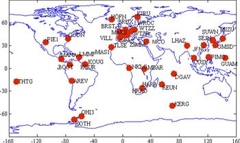
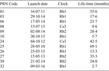
To show the application of the GPS triple-frequency satellite clock offset and analyse the characteristics of the biases, a one-month (1–30 April 2016) triple-frequency GPS data set from 40 IGS stations was processed to estimate the triple-frequency satellite clock offset. Data was sampled at 30 s and the cut-off elevation was set at 10°. Figure 2 shows the distribution of the 40 stations used. To date, 12 BLOCK IIF satellites have been in operation. The information of these 12 BLOCK IIF satellites is shown in Table 1.
Distribution of the 40 IGS stations tracking GPS triple-frequency signals.

Information of the GPS BLOCK IIF satellites.

4.1. Performance of the DCBs
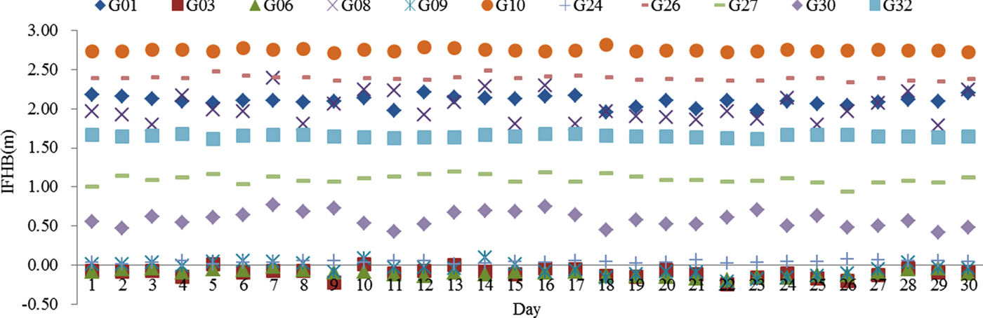
It is very important to obtain the DCB(P1-P2), DCB(P1-P5) and IFCB for the “Service” and the “Estimation” of the GPS triple-frequency satellite clock offsets. The estimation method for the constant part (Inter-frequency Hardware Bias, IFHB) and variable part of the IFCB is presented in Li et al. (Reference Li, Li, Xiao, Wang and Xu2016b). The IFCB and IFHB of the five BLOCK IIF satellites (PRN01, PRN24, PRN25, PRN27 and PRN30) were analysed. To further study the suitability of the IFCB and IFHB estimation method for all BLOCK IIF satellites, the IFCB and IFHB for these 12 BLOCK IIF satellites were computed according to Li et al. (Reference Li, Li, Xiao, Wang and Xu2016b). For the processing, the PRN25 is selected as the reference satellite. The estimated IFHB results are illustrated in Figure 3.
Satellite IFHBs with PRN25 as reference satellite over one month.

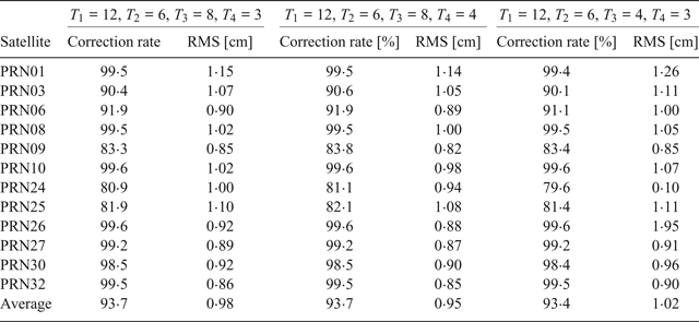
Figure 3 shows that the satellite IFHBs of each satellite are different. The satellite IFHBs of PRN03, PRN06 and PRN09 with PRN25 as reference satellite in Figure 3 are very small, which means that the satellite IFHBs of PRN03, PRN06 and PRN09 are very close. The one-month daily IFHBs show that they are stable in the short term. The IFCB is then determined and for this purpose the combined linear and fourth harmonic function is used to model the IFCB. The harmonic coefficients, θi and λi(i=1~4), of different groups are estimated by employing the least squares method for a 24-h data arc. Inserting the estimated coefficients and related periods, T i(i=1~4), into Equation (9), the modelled IFCBs can be deduced. Comparing the modelled values with the estimated ones, the correction rates of different period groups are computed. The averages of the single-day correction rates and Root Mean Square (RMS) over one month for different options for the period groups (T i) are also shown in Table 2.
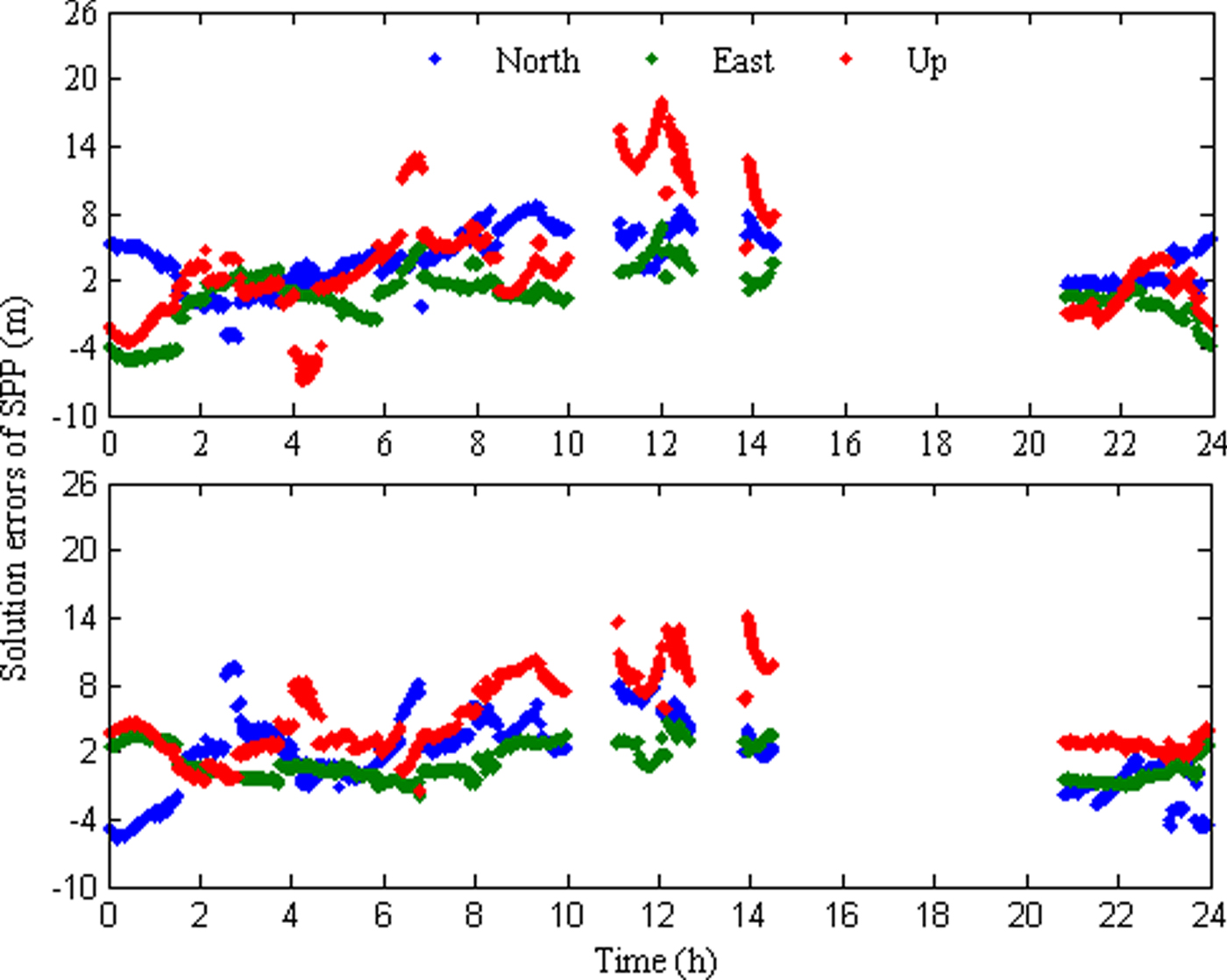
SPP solution errors, when the biases (DCB(P1-P5) and modelled IFCB) is not used (top) and used (bottom).

Mean of correction rates and RMS for different groups of periods.

Table 2 indicates that the correction accuracies of all models are better than 1.02 cm. The correction rates and correction accuracies show that the model with the periods of 12, 6, 8 and 4 h yield the best performance with respect to other period groups, with an accuracy better than 0.95 cm and a correction rate better than 81.1%.
4.2. Performance of the estimated satellite clocks offsets
In data processing, the L1/L2 and P1/P2 observations are selected as the reference observation. So, the IGS final satellite clock product is used. Based on the IGS satellite clock and bias products (DCB(P1-P2), DCB(P1-P5) and modelled IFCB), the triple-frequency satellite clock offset is computed. Code observation-based Single Point Positioning (SPP) is sensitive to the bias of the estimated satellite clock offset so that the five-day (26–30 April 2016) triple-frequency GPS data is collected in Urumqi and processed using SPP mode. Data was sampled at 30 s and the cut-off elevation was set at 10°. In processing, the elevation-dependent weights for the code observations were determined:
 $$w(\theta ) = \left\{\matrix{1 \hfill & 30^0 \le \theta \le 90^0 \hfill \cr 2\sin (\theta) \hfill &10^0 \le \theta \lt 30^0 \hfill}\right.$$
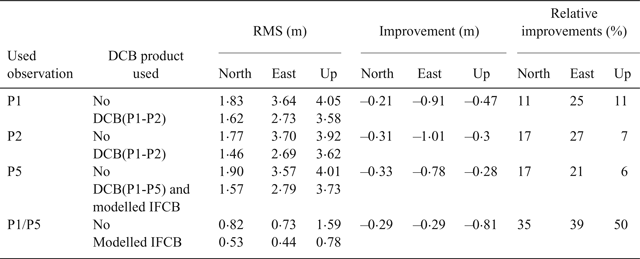
where θ is the satellite elevation. The corrections, Earth tides, relativistic effects and antenna phase centre offsets are implemented. The tropospheric and ionospheric delays are corrected using the Saastamoinen and Klobuchar models (Leick et al., Reference Leick, Rapoport and Tatarnikov2015). A least squares estimator is used to solve the epoch-wise coordinates. The averages of the five-day RMS values of SPP solution errors with respect to the ground truth coordinates are computed for the coordinate components North, East and Up, as shown in Table 3. When the P5 code observation is processed, the SPP solution errors on 26 April 2016 are illustrated in Figure 4.
Averages of the five-day RMSs of SPP solution of different strategies.

From Table 3 and Figure 4, it is observed that significant improvements are achieved in all three coordinate components, when the bias products (DCB(P1-P2), DCB(P1-P5) and modelled IFCB) are used. The improvements are similar for all the strategies and the effect of the biases (DCB(P1-P2), DCB(P1-P5) and modelled IFCB) on the vertical direction is more evident than on the horizontal directions. On average, the relative improvements are about 20%, 28% and 19% for north, east and vertical components. To date, 12 BLOCK IIF satellites have been in operation and less than six BLOCK IIF satellites are visible at a time, which is hardly sufficient to demonstrate effectively the continuous benefit of the proposed approach to positioning. The results further show the role and significance of the biases (DCB(P1-P2), DCB(P1-P5) and IFCB) in the triple-frequency satellite clock offset estimation.
5. CONCLUSION AND DISCUSSION
Due to the satellite bias between the observations and its contribution to the estimated satellite clock offset, there are differences between the satellite clock offsets estimated with different observations. To compute the satellite clock offsets of the different observations, the reference observations are firstly selected, and the corresponding satellite clock offset is estimated. Then, based on the estimated values of the reference observations and the biases between the reference observations and other observations, the satellite clock offsets for all observations are obtained. The current IGS GPS satellite clock offset biases on the reference of L1/L2 and P1/P2 and the satellite clock offsets of P1(L1) and P2(L2) are computed using the DCB(P1-P2) product. With the development of multiple GNSSs, signals on three or more carrier frequencies are broadcast. A variable bias can be observed between the triple-frequency observations, and this is named IFCB, since the reference observations are different. The variable IFCB leads to an increased service complexity. However, it can be seen that the combined linear and fourth order harmonic function can well describe IFCB and the 14-coefficient function can replace the IFCB series. The provision of those coefficients avoids providing the IFCB series. This can greatly reduce communication network loads. In application of the GPS triple-frequency satellite clock offsets, the performances of the satellite biases (DCB(P1-P2), DCB(P1-P5) and modelled IFCB) are discussed. One-month daily IFHBs indicate that they are stable in the short term. The IFCB modelling demonstrates that the correction accuracies of all models are better than 1·02 cm. The correction rates and correction accuracies (RMS) indicate that the model with the periods of 12, 6, 8 and 4 h is better than other ones, its accuracy reaches mm level and the correction rate is better than 81·1%. The estimated GPS triple-frequency satellite clock offsets are evaluated using its performance in SPP. The SPP results indicate that significant improvements are achieved in all three coordinate components, when the bias products (DCB(P1-P2), DCB(P1-P5) and modelled IFCB) are considered in GPS triple-frequency satellite clock offset estimation. The effect of the biases (DCB(P1-P2), DCB(P1-P5) and modelled IFCB) on the vertical direction is more evident than on the horizontal directions.
ACKNOWLEDGMENTS
This research is supported by the National Natural Science Foundation of China (NSFC) (No: 41674029), Science and Technology Commission of Shanghai Municipality (No. 17DZ1100902), the Key R&D Program (2016YFB0501701), the National High Technology Research and Development Program of China (No: 2014AA123102), the Projects of Science and Technology Commission of Shanghai Municipality (No: 140302) and the State Key Development Program for Basic Research of China (No. 2013CB733304)