





1. Introduction
Drag reduction (DR) is a long-standing goal in both fundamental fluid mechanics and engineering practice. Among the available strategies two have proven particularly effective. The first relies on stratifying the flow with a thin, less viscous lubricating film near the wall, which carries most of the shear and shields the bulk fluid from direct contact with the solid boundary; this idea, originally motivated by the pipeline transport of heavy crude oils, has been extensively characterised both experimentally and numerically (Isaac & Speed Reference Isaac and Speed1904; Looman Reference Looman1916; Joseph et al. Reference Joseph, Renardy and Renardy1984, Reference Joseph, Bai, Chen and Renardy1997; Hu & Joseph Reference Hu and Joseph1989; Kim & Choi Reference Kim and Choi2018; Roccon et al. Reference Roccon, Zonta and Soldati2024). The second exploits the rheological properties of dilute polymer solutions: small amounts of polymers dissolved in a Newtonian solvent can modify the near-wall turbulence and lead to dramatic reductions of frictional losses (Forrest & Grierson Reference Forrest and Grierson1931; Virk Reference Virk1975; White & Mungal Reference White and Mungal2008; Wang et al. Reference Wang, Yu, Zakin and Shi2011). In a previous work (Milocco et al. Reference Milocco, Roccon and Soldati2026), we combined these two mechanisms by lubricating a turbulent Newtonian channel flow with a thin non-Newtonian layer injected in the near-wall region. That study, however, was carried out at a single value of the Weissenberg number, leaving open the question of how the elasticity of the lubricating layer controls the DR performance. For single-phase polymer solutions, it is well established that DR does not grow indefinitely with polymer concentration or elasticity, but is bounded by the maximum DR asymptote of Virk (Reference Virk1975). Whether an analogous upper bound exists for DR via a viscoelastic lubricating layer is the main question of this work.
Despite their practical importance, multiphase flows involving non-Newtonian fluids have received relatively limited attention. While a substantial body of work exists on single-phase non-Newtonian laminar and turbulent flows (Arosemena et al. Reference Arosemena, Andersson and Solsvik2021; Amor et al. Reference Amor, Soligo, Mazzino and Rosti2024; Serafini et al. Reference Serafini, Battista, Gualtieri and Casciola2024; Milocco et al. Reference Milocco, Giamagas, Zonta and Soldati2025; Rosti Reference Rosti2025; Xu et al. Reference Xu, Zhang, Brandt, Song and Shishkina2025), far fewer studies have addressed multiphase systems. Most existing studies have examined the dynamics, deformation and interaction of drops and bubbles in non-Newtonian fluids or the other way around (Oishi et al. Reference Oishi, Martins, Tomé and Alves2012; Yue & Feng Reference Yue and Feng2012; Wang et al. Reference Wang, Do-Quang and Amberg2017; Amani et al. Reference Amani, Balcázar, Castro and Oliva2019; Balasubramanian et al. Reference Balasubramanian, Sanjay, Jalaal, Vinuesa and Tammisola2024; Iqbal et al. Reference Iqbal, Izbassarov, Brandt and Tammisola2026), with only a small number addressing turbulent conditions (Rosti & Brandt Reference Rosti and Brandt2017; Del Gaudio et al. Reference Del Gaudio, Constantinescu, Di Cristo, De Paola and Vacca2024). This is largely due to the numerical challenges associated with the solution of the conformation tensor equation, which is required to describe viscoelastic non-Newtonian fluids: a central difficulty stems from the requirement that the conformation tensor remain symmetric positive definite at all times to retain its physical meaning, a constraint that is hard to enforce numerically and that becomes even more demanding in multiphase configurations, where deformable interfaces introduce sharp jumps in fluid properties and viscoelastic parameters that interact non-trivially with the polymer stress field.
In this work, we build on our previous study (Milocco et al. Reference Milocco, Roccon and Soldati2026), in which we performed direct numerical simulations of the turbulent flow of a main layer lubricated by a non-Newtonian layer, comparing four rheological models for the lubricant: Newtonian, shear-thinning (Carreau), combined shear-thinning and viscoelastic (FENE-P) and purely viscoelastic (FENE-CR). That work showed that – in line with previous findings for Newtonian–Newtonian configurations (Roccon et al. Reference Roccon, Zonta and Soldati2019) – surface tension provides a substantial contribution to DR, but viscoelasticity plays an equally important role: both FENE-P and FENE-CR lubricating layers double the DR performance relative to the Newtonian-lubricating-layer case. In contrast, shear-thinning effects lead only to marginal gains. Motivated by these preliminary findings, we perform a new campaign of high-resolution simulations aimed at unveiling the effects of elasticity on DR. With this aim, we consider here a turbulent channel flow at
 $\textit{Re}_\tau = 300$
lubricated by a purely viscoelastic lubricating layer (FENE-CR model) having the same density and zero-shear viscosity as the main transported layer. The lubricating-layer thickness is set to
 $90\,\mathrm{w.u.}$
such that, in the Newtonian limit, the layer sustains fully developed turbulence (Jiménez & Moin Reference Jiménez and Moin1991; Orlandi et al. Reference Orlandi, Bernardini and Pirozzoli2015; Roccon et al. Reference Roccon, Zonta and Soldati2019), thereby enabling the effect of elasticity on an already turbulent state to be isolated. We consider different elasticity levels, determined by the shear Weissenberg number
 $\textit{Wi}_\tau$
, ranging from the Newtonian limit (
 $\textit{Wi}_\tau = 0$
) to a highly elastic case (
 $\textit{Wi}_\tau = 100$
). Global quantities and turbulence statistics are employed to quantify the DR performance and its modifications due to elasticity. Subsequently, starting from the transport equations for the interfacial energy and the elastic potential energy (EPE), we extend and apply the energy-box framework (Ricco et al. Reference Ricco, Ottonelli, Hasegawa and Quadrio2012; Gatti et al. Reference Gatti, Cimarelli, Hasegawa, Frohnapfel and Quadrio2018; Andreolli et al. Reference Andreolli, Quadrio and Gatti2021; Roccon et al. Reference Roccon, Zonta and Soldati2021) to non-Newtonian multiphase systems. This framework graphically displays the fluxes associated with the budgets of mean kinetic, turbulent kinetic and elastic potential energy. The comparison of the energy boxes obtained for the different cases allows us to identify the physical mechanism responsible for the observed saturation of DR. In particular, by comparing the relative importance of the different energy-transfer pathways, we show how increasing elasticity progressively alters the redistribution of energy throughout the system, ultimately leading to a self-limiting DR mechanism.
2. Methodology
We consider a channel flow configuration consisting of two immiscible fluid layers, one above the other. The main Newtonian layer, which has a nominal thickness of
 $h_m = 1.7h$
, is lubricated by a thin purely viscoelastic layer with a nominal thickness of
 $h_l = 0.3h$
. The channel has dimensions
 $L_{x} \times L_{y} \times L_{z} = 4\pi h \times 2\pi h \times 2h$
, where
 $h$
is the half-channel height and
 $x$
,
 $y$
and
 $z$
are the streamwise, spanwise and wall-normal directions, respectively. To capture the dynamics of the two-phase flow, we perform direct numerical simulations of the incompressible Navier–Stokes equations coupled with a diffuse-interface phase-field method, based on a Cahn–Hilliard equation (Jacqmin Reference Jacqmin1999; Badalassi et al. Reference Badalassi, Ceniceros and Banerjee2003; Roccon et al. Reference Roccon, Zonta and Soldati2023). When the lubricating layer is viscoelastic, an additional transport equation for the polymer conformation tensor is solved.
2.1. Phase-field method
The dynamics of the deformable interface is described using a phase-field method, which relies on an order parameter (phase field)
 $\phi$
such that
 $\phi = 1$
in the main Newtonian layer and
 $\phi = -1$
in the viscoelastic lubricating layer. The phase-field variable varies smoothly across a thin interfacial region between these two bulk values. The evolution of
 $\phi$
is governed by the Cahn–Hilliard equation, which in dimensionless form reads
 \begin{align} \frac {\partial \phi }{\partial t} + \boldsymbol{u}\boldsymbol{\cdot }\boldsymbol{\nabla }\phi = \frac {1}{\textit{Pe}_\phi }\,{\nabla} ^2 \mu _\phi, \end{align}
where
 $\boldsymbol{u}=(u,v,w)$
is the velocity vector and
 $\textit{Pe}_\phi = u_\tau h/(\mathcal{M}\beta )$
is the Péclet number, quantifying the ratio between convective and diffusive time scales of the interface;
 $u_\tau$
is the friction velocity,
 $\mathcal{M}$
is the mobility and
 $\beta$
is a constant introduced to make the chemical potential dimensionless (Jacqmin Reference Jacqmin1999; Soligo et al. Reference Soligo, Roccon and Soldati2019). The chemical potential
 $\mu _\phi$
is defined as the variational derivative of the Ginzburg–Landau free-energy functional:
 \begin{align} \mu _\phi = \frac {\delta \mathcal{F}[\phi ,\boldsymbol{\nabla }\phi ]}{\delta \phi }, \end{align}
which collects the thermodynamic driving forces responsible for phase separation and interfacial dynamics. For an immiscible binary mixture with a viscoelastic phase, we adopt the following functional (Jacqmin Reference Jacqmin1999; Yue et al. Reference Yue, Feng, Liu and Shen2004, Reference Yue, Feng, Liu and Shen2005):
 \begin{align} \mathcal{F}[\phi ,\boldsymbol{\nabla }\phi ] = \int _{\varOmega }\left (\frac {(\phi ^2-1)^2}{4} + \frac {\textit{Ch}^2}{2}\,|\boldsymbol{\nabla }\phi |^2 + \frac {1-\phi }{2}\frac {1-x_0}{\textit{Wi}_\tau } \int _{\mathbb{R}^3} \psi \left ( \ln \psi + \frac {1}{2} \boldsymbol{q} \boldsymbol{\cdot }\boldsymbol{q} \right ) \, {\rm d}\boldsymbol{q}\right )\,{\rm d}\varOmega , \end{align}
where
 $\varOmega$
is the computational domain and
 $\textit{Ch}=\xi /h$
is the Cahn number. The first contribution is a double-well potential, with minima at
 $\phi =\pm 1$
, promoting separation into the two pure phases. The second term penalises gradients of
 $\phi$
and therefore accounts for interfacial (mixing) energy, setting both the interface thickness and the surface-tension-related forcing. The third term represents an elastic free-energy contribution associated with polymer deformation, expressed through the probability density function
 $\psi (\boldsymbol{q})$
of the polymer end-to-end vector
 $\boldsymbol{q}$
; the prefactor
 $(1-\phi )/2$
confines this contribution to the viscoelastic layer. Taking the variational derivative of (2.3) yields
 \begin{align} \mu _\phi = \phi ^3 - \phi - \textit{Ch}^2 {\nabla} ^2 \phi + \frac {\delta f_e}{\delta \phi }, \end{align}
where
 $\delta f_e/\delta \phi$
is the contribution arising from the elastic term present in (2.3). This elastic contribution becomes asymptotically negligible in the sharp-interface limit (
 $\textit{Ch}\to 0$
), as elastic stresses act at leading order only through the momentum equation and do not modify the equilibrium interfacial structure (Yue et al. Reference Yue, Feng, Liu and Shen2004, Reference Yue, Feng, Liu and Shen2005; Milocco et al. Reference Milocco, Roccon and Soldati2026). With this assumption, the last term in (2.4) can be neglected, and the chemical potential retains the standard form used in Newtonian flows.
2.2. Hydrodynamics and viscoelastic rheology
The hydrodynamics of the two-phase flow is described by coupling the Cahn–Hilliard equation with the incompressible Navier–Stokes equations within a one-fluid formulation (Prosperetti & Tryggvason Reference Prosperetti and Tryggvason2007). In this approach, a single set of governing equations is solved over the entire domain, while the presence of a deformable interface and the accompanying surface tension forces are accounted for by introducing a capillary term. The resulting mass conservation and momentum equations, in dimensionless form, read as follows:
 \begin{align} \boldsymbol{\nabla }\boldsymbol{\cdot }\boldsymbol{u} = 0, \end{align}
 \begin{align} \frac {\partial \boldsymbol{u}}{\partial t} + \boldsymbol{u}\boldsymbol{\cdot }\boldsymbol{\nabla }\boldsymbol{u} = -\boldsymbol{\nabla }\!p &+ \frac {x_0}{\textit{Re}_\tau }\, \boldsymbol{\nabla }\boldsymbol{\cdot }\!\left [ \left (1+\frac {(1/x_0-1)(\phi +1)}{2}\right ) \left (\boldsymbol{\nabla }\boldsymbol{u}+\boldsymbol{\nabla }\boldsymbol{u}^{{T}}\right ) \right ] \nonumber\\[5pt] & + \frac {1-x_0}{\textit{Re}_\tau }\,\boldsymbol{\nabla }\boldsymbol{\cdot }\boldsymbol{\tau }_p + \frac {3\,\textit{Ch}}{\sqrt {8}\,\textit{We}}\,\boldsymbol{\nabla }\boldsymbol{\cdot }\boldsymbol{\tau }_c , \end{align}
where
 $p$
is the pressure field,
 $x_0$
the solvent-to-total viscosity ratio (discussed later) and
 $\boldsymbol{\tau }_p$
the polymer stress tensor. The capillary stress tensor
 $\boldsymbol{\tau }_c$
is defined as follows:
 \begin{align} \boldsymbol{\tau }_c = |\boldsymbol{\nabla }\phi |^2\,\boldsymbol{I} - \boldsymbol{\nabla }\phi \otimes \boldsymbol{\nabla }\phi , \end{align}
in accordance with the Korteweg formulation (Korteweg Reference Korteweg1901). The governing parameters are the shear Reynolds number
 $\textit{Re}_\tau =\rho u_\tau h/\mu _m$
, based on the viscosity
 $\mu _m$
of the Newtonian main layer, and the Weber number
 $\textit{We}=\rho u_\tau ^2 h/\sigma$
, which quantifies the ratio between inertial and surface-tension forces. In (2.6), the first stress term represents the solvent contribution, whose effective viscosity varies smoothly across the interface through the phase-field variable, while the second term accounts for the polymeric contribution associated with the viscoelastic lubricating layer. This formulation ensures a smooth transition between the properties of the fluids in the context of a single-fluid formulation. In particular, when
 $x_0=1$
the polymeric contribution vanishes identically and the momentum equation reduces to the classical incompressible Navier–Stokes equations for a Newtonian fluid with uniform viscosity. For the FENE-CR model, the polymer stress tensor
 $\boldsymbol{\tau }_p$
is defined as follows:
 \begin{align} \boldsymbol{\tau }_p = \frac {\textit{Re}_\tau }{\textit{Wi}_\tau } f(\boldsymbol{C})\left (\boldsymbol{C}-\boldsymbol{I}\right )\!, \end{align}
where
 $\boldsymbol{C}$
is the polymer conformation tensor and
 $\textit{Wi}_\tau =\rho \lambda u_\tau ^2/\mu _0$
is the shear Weissenberg number, with
 $\lambda$
denoting the polymer relaxation time. Finite extensibility effects are incorporated through
 \begin{align} f(\boldsymbol{C})=\frac {L^2}{L^2-\mathrm{tr}(\boldsymbol{C})}, \end{align}
where
 $L$
is the extensibility limit. The evolution of the conformation tensor is governed by the following equation:
 \begin{align} \frac {\partial \boldsymbol{C}}{\partial t} + \boldsymbol{u}\boldsymbol{\cdot }\boldsymbol{\nabla }\boldsymbol{C} = \boldsymbol{C}\boldsymbol{\cdot }\boldsymbol{\nabla }\boldsymbol{u} + \left (\boldsymbol{C}\boldsymbol{\cdot }\boldsymbol{\nabla }\boldsymbol{u}\right )^{\text{T}} -\frac {1-\phi }{2\,\textit{Wi}} f(\boldsymbol{C})\left (\boldsymbol{C}-\boldsymbol{I}\right ) + \frac {1}{\textit{Re}_\tau \,\textit{Sc}_{\!p}}\,{\nabla} ^2\boldsymbol{C}, \end{align}
where
 $\textit{Wi}=\textit{Wi}_\tau /\textit{Re}_\tau$
and
 $\textit{Sc}_{\!p}=\mu _0/(\rho k)$
is the polymer Schmidt number controlling the strength of the diffusive regularisation term (Sureshkumar et al. Reference Sureshkumar, Beris and Handler1997; Dimitropoulos et al. Reference Dimitropoulos, Sureshkumar and Beris1998; Xi & Graham Reference Xi and Graham2010; Alves et al. Reference Alves, Oliveira and Pinho2021; Milocco et al. Reference Milocco, Roccon and Soldati2026). In the Newtonian layer, the relaxation term vanishes and the conformation tensor remains close to its equilibrium configuration,
 $\boldsymbol{C}\approx \boldsymbol{I}$
. In contrast, within the viscoelastic lubricating layer the full polymer dynamics is active, generating elastic stresses that interact with turbulence and interfacial motion. Additional details on the employed methodology can be found in Milocco et al. (Reference Milocco, Roccon and Soldati2026).
2.3. Numerical method
Equations (2.1), (2.5), (2.6) and (2.10) are solved using FLOW36, an open-source, GPU-ready pseudo-spectral solver (Roccon et al. Reference Roccon, Soligo and Soldati2025). Spatial discretisation is based on Fourier expansions in the two homogeneous directions (
 $x$
and
 $y$
) and Chebyshev polynomials in the wall-normal direction (
 $z$
). The Navier–Stokes equations are solved using the wall-normal velocity–vorticity formulation (Kim et al. Reference Kim, Moin and Moser1987; Speziale Reference Speziale1987), which results in a fourth-order equation for the wall-normal velocity
 $w$
and a second-order equation for the wall-normal vorticity
 $\omega _z$
. The Cahn–Hilliard equation is reformulated as two coupled second-order equations (Badalassi et al. Reference Badalassi, Ceniceros and Banerjee2003). Time integration is performed using an implicit–explicit scheme (Moin & Kim Reference Moin and Kim1980). For the momentum equations, linear terms are treated implicitly with a Crank–Nicolson scheme, while nonlinear terms are advanced explicitly using a second-order Adams–Bashforth method. For the Cahn–Hilliard equation, the linear contribution is integrated implicitly using backward Euler to enhance numerical stability and suppress high-frequency oscillations, whereas the nonlinear terms are treated explicitly with Adams–Bashforth (Yue et al. Reference Yue, Feng, Liu and Shen2004). For the conformation tensor transport equation, the diffusive regularisation term is integrated implicitly via Crank–Nicolson, while all remaining terms are advanced explicitly, in line with standard pseudo-spectral treatments of viscoelastic flows (Sureshkumar et al. Reference Sureshkumar, Beris and Handler1997; Dimitropoulos et al. Reference Dimitropoulos, Sureshkumar and Beris1998; Xi & Graham Reference Xi and Graham2010). To prevent loss of positive definiteness of the conformation tensor and enforce the finite-extensibility constraint
 $\mathrm{tr}(\boldsymbol{C})\lt L^2$
, we employ the boundedness-preserving strategy originally proposed by Vaithianathan & Collins (Reference Vaithianathan and Collins2003) and subsequently refined by Dubief et al. (Reference Dubief, Terrapon, White, Shaqfeh, Moin and Lele2005) and Richter et al. (Reference Richter, Iaccarino and Shaqfeh2010). In this approach, an auxiliary variable related to the finite-extensibility function is evolved in place of
 $\boldsymbol{C}$
when evaluating the nonlinear terms, ensuring numerical stability of the polymer configuration.
2.4. Simulations
We perform direct numerical simulations of a turbulent channel flow configuration at a nominal friction Reynolds number
 $\textit{Re}_\tau =300$
and considering a fixed value of the Weber number
 $\textit{We}=0.5$
. Viscoelastic effects in the lubricating layer are governed solely by the shear Weissenberg number
 $\textit{Wi}_\tau$
and the following values have been considered:
 $\textit{Wi}_\tau = 25,\ 50,\ 75$
and
 $100$
. The Cahn number is set equal to
 $\textit{Ch}=0.02$
, and the Péclet number is set following the scaling
 $\textit{Pe}_\phi =3/\textit{Ch}=150$
to ensure convergence to the sharp-interface limit (Magaletti et al. Reference Magaletti, Picano, Chinappi, Marino and Casciola2013). The solvent-to-total-viscosity ratio is fixed to
 $x_0=0.9$
, and the zero-shear viscosity of the lubricating layer is matched to that of the Newtonian main layer,
 $\mu _0=\mu _m$
. The polymer extensibility parameter is set to
 $L=30$
. The Schmidt number, which controls the amplitude of the regularisation term in the conformation tensor equation, is set to
 $\textit{Sc}_{\!p}=1$
for
 $\textit{Wi}_\tau =25$
and
 $50$
, and slightly reduced to
 $\textit{Sc}_{\!p}=0.95$
for
 $\textit{Wi}_\tau =75$
and
 $100$
to enhance numerical stability. As shown by Milocco et al. (Reference Milocco, Roccon and Soldati2026), variations of
 $\textit{Sc}_{\!p}$
have negligible impact on conformation-tensor statistics and global flow quantities. An overview of the simulation parameters is reported in table 1. A constant pressure gradient is used to drive the flow along the streamwise direction.
Overview of the main simulation parameters. Six simulations have been performed: a single-phase reference case, a Newtonian–Newtonian lubricated case and four viscoelastic lubricated cases (FENE-CR). All simulations are driven by a constant pressure gradient.

Table 1. Long description
The table presents an overview of simulation parameters for six different flow configurations. It has six rows and eight columns. The columns are labeled as System, Wi_tau, Re_tau, We, Ch, Sc_p, and N_x x N_y x N_z. The rows are labeled as Single phase, Lubricated (Newtonian), Lubricated (FENE-CR) with different Wi_tau values (25, 50, 75, 100). Each row lists specific values for the parameters Wi_tau, Re_tau, We, Ch, Sc_p, and the grid dimensions N_x x N_y x N_z. The table compares these parameters across different simulation setups, highlighting variations in viscoelastic effects and lubrication conditions.
The single-phase and Newtonian–Newtonian simulations employ a grid resolution equal to
 $512\times 256\times 257$
in the streamwise, spanwise and wall-normal directions, respectively. On the other hand, all viscoelastic lubricated simulations are performed on a refined grid of
 $512\times 512\times 513$
points. The increased resolution is required to ensure numerical stability in the solution of the conformation-tensor equation and to accurately resolve sharp gradients of the polymer stresses near the wall and the interface (Thais et al. Reference Thais, Gatski and Mompean2013; Milocco et al. Reference Milocco, Roccon and Soldati2026). Since the FENE-CR model represents a purely viscoelastic fluid with constant viscosity, the refinement is not associated with shear-dependent viscosity variations, but with the accurate resolution of polymer-stress fluctuations. The same grid is adopted for all viscoelastic cases to ensure consistent spatial resolution.
Periodic boundary conditions are enforced along the two homogeneous directions (
 $x$
and
 $y$
). At the two walls (
 $z/h=\pm 1$
), no-slip conditions are imposed on the velocity field while no-flux conditions are prescribed for the phase field and the corresponding chemical potential (Jacqmin Reference Jacqmin1999; Yue et al. Reference Yue, Feng, Liu and Shen2004). The boundary conditions for the conformation tensor depend on the local rheology. At the top wall (
 $z/h=1$
), where the fluid is Newtonian, the polymer configuration is set to its equilibrium (coiled) state,
 $\boldsymbol{C}=\boldsymbol{I}$
. At the bottom wall (
 $z/h=-1$
), where the viscoelastic lubricating layer is present, vanishing artificial diffusivity is assumed (
 $\textit{Sc}_{\!p}\to \infty$
) and the conformation tensor is advanced explicitly in time using a second-order Adams–Bashforth scheme on the nonlinear terms of (2.10) (Dimitropoulos et al. Reference Dimitropoulos, Sureshkumar and Beris1998; Milocco et al. Reference Milocco, Roccon and Soldati2026). This treatment ensures that polymer stresses remain confined to the viscoelastic layer and evolve consistently with the interface dynamics.
A single-phase turbulent channel flow simulation is first performed and then used to initialise all lubricated channel flow simulations. These simulations are initialised considering two liquid layers separated by a flat interface located at a distance
 $0.3h$
from the bottom wall (leading to a lubricating-layer thickness equal to
 $90\,\mathrm{w.u.}$
), as shown in figure 1. The initial condition for the phase-field variable is
 \begin{align} \phi (x,y,z) = -\tanh \left (\frac {h_l/h-1-z/h}{\sqrt {2}\,\textit{Ch}}\right )\!, \end{align}
where
 $h_l$
is the lubricating layer thickness in outer units (
 $0.3h$
). The conformation tensor for the viscoelastic simulations is initialised with zero polymer stress, corresponding to
 $\boldsymbol{C}=\boldsymbol{I}$
throughout the domain. Before collecting statistics, each simulation is advanced until a statistically stationary state is reached. All statistical quantities reported in the following are computed over an averaging interval
 $\Delta t^+ \geqslant 4000$
.
Instantaneous visualisations of lubricated turbulent flows for increasing elasticity values of the lubricating layer: Newtonian (left), weakly elastic (
 $\textit{Wi}_\tau =50$
; centre) and highly elastic (
 $\textit{Wi}_\tau =100$
; right). The greyscale colour map (white to black) represents the streamwise velocity, while the yellow-to-blue colour map shows the EPE. The two close-up views illustrate the interfacial waves, with the red line denoting the mean interface position. An increase in polymer relaxation time leads to a more homogeneous distribution of EPE, which depends directly on polymer stretching, and results in smoother interfacial waves.

3. Results
In this section, we examine how the elasticity of the lubricating layer influences macroscopic observables – namely, flow rates and mean flow – as well as turbulence statistics and energy fluxes in the multiphase system. Unless stated otherwise, angular brackets
 $\langle \boldsymbol{\cdot }\rangle$
denote averaging over the homogeneous directions
 $(x,y)$
, while square brackets
 $[\boldsymbol{\cdot }]$
denote averaging over
 $(x,y)$
and time. Flow quantities are decomposed into mean and fluctuating components using a standard Reynolds decomposition (Reynolds Reference Reynolds1895). Thus a generic field
 $f(x,y,z,t)$
can be decomposed as follows:
 \begin{align} f(x,y,z,t) = \langle f(z,t) \rangle + f'(x,y,z,t), \end{align}
where the mean component depends only on the wall-normal coordinate and time. The results are organised as follows. We begin by examining the impact of the lubricating layer on the mean streamwise velocity profiles and Reynolds stresses. We then analyse the budgets of mean and turbulent kinetic energy, along with the polymer elastic energy in the lubricating layer. These energy transfer mechanisms are summarised graphically using the energy-box framework (Ricco et al. Reference Ricco, Ottonelli, Hasegawa and Quadrio2012; Gatti et al. Reference Gatti, Cimarelli, Hasegawa, Frohnapfel and Quadrio2018; Roccon et al. Reference Roccon, Zonta and Soldati2021). The analysis is performed separately within each phase, enabling a careful characterisation of the energy fluxes exchanged across the deformable interface and within each layer. Finally, the self-limiting DR mechanism associated with elasticity, identified through the energy-box framework, is summarised in the last section, where the behaviour of key quantities is shown as a function of elasticity.
3.1. Drag reduction performance and turbulence statistics
We start our discussion by examining the mean-flow behaviour (figure 2). Unless otherwise stated, results are reported using the following colour scheme: single-phase turbulent flow (black), Newtonian lubricating layer (blue) and viscoelastic lubricating layers with
 $\textit{Wi}_\tau = 25$
(purple),
 $\textit{Wi}_\tau = 50$
(magenta),
 $\textit{Wi}_\tau = 75$
(red) and
 $\textit{Wi}_\tau = 100$
(yellow). Figure 2(
 $a$
) shows the wall-normal behaviour of the mean streamwise velocity profiles. The single-phase reference is included for comparison, and the nominal interface location at
 $z/h=-0.7$
is indicated by a vertical grey dashed line. First, we observe that the presence of a lubricating layer in the bottom part of the channel creates a strong asymmetry in the mean velocity profiles with respect to the channel centreline. All lubricated configurations exhibit an increase of the mean velocity in the main layer, indicating the presence of DR (as the flow is driven by a constant mean pressure gradient). For the Newtonian case, this increase is moderate and primarily associated with a redistribution of the mean shear across the channel. When the lubricating layer is viscoelastic, the mean velocity increase becomes more pronounced, with its magnitude depending on the considered elasticity value, as can be also appreciated from the darker colours obtained in figure 1 for the viscoelastic cases (centre and right). Notably, an increase of the Weissenberg number leads to a systematic increase of the mean velocity profile in the main layer. This increase is monotonic with
 $\textit{Wi}_\tau$
, with higher elasticity corresponding to larger bulk velocities. However, the incremental gain decreases as
 $\textit{Wi}_\tau$
increases. The separation between the
 $\textit{Wi}_\tau =25$
and
 $\textit{Wi}_\tau =50$
profiles is appreciable, whereas the additional increase obtained at
 $\textit{Wi}_\tau =75$
and
 $100$
is comparatively small.
(
 $a$
) The mean streamwise velocity profiles for a Newtonian main layer and lubricating layers of increasing elasticity. The single-phase turbulent flow is shown in black, while the lubricated cases correspond to increasing
 $\textit{Wi}_\tau$
. The nominal interface location at
 $z/h=-0.7$
is indicated by a vertical dashed line. (
 $b$
) The corresponding flow rates. The total flow rate
 $Q_{{tot}}/Q_{SP}$
(filled symbols) and the contribution of the main Newtonian layer
 $Q_{m}/Q_{SP}$
(open symbols) are shown as functions of the Weissenberg number
 $\textit{Wi}_\tau$
. All quantities are normalised by the corresponding single-phase value
 $Q_{SP}$
. The case
 $\textit{Wi}_\tau =0$
identifies the Newtonian case.

Figure 2. Long description
Panel A: A line graph shows the mean streamwise velocity profiles for a Newtonian main layer and lubricating layers of increasing elasticity. The x-axis represents the normalized height (z/h), and the y-axis represents the velocity (u). The single-phase turbulent flow is depicted in black, while the lubricated cases correspond to increasing Weissenberg numbers (Wi_tau) in different colors. The nominal interface location at z/h = 0 is indicated by a vertical dashed line. Panel B: Another line graph shows the corresponding flow rates. The x-axis represents the Weissenberg number (Wi_tau), and the y-axis represents the normalized flow rate (Q/Q_SP). The total flow rate is shown with filled symbols, and the contribution of the main Newtonian layer is shown with open symbols. The flow rates increase with the Weissenberg number, with the total flow rate showing a more significant increase compared to the Newtonian layer’s contribution.
A quantitative measure of the DR performance obtained for the different cases is provided in figure 2(
 $b$
), where the normalised total flow rate
 $Q_{{tot}}/Q_{SP}$
and the contribution of the main layer
 $Q_m/Q_{SP}$
are plotted as functions of the elasticity of the lubricating layer. Because all simulations are driven using a constant-pressure-gradient approach, DR is reported as the relative increase in total flow rate with respect to the single-phase case
 $\Delta Q = (Q_{{tot}}/Q_{SP}-1)\times 100\,\%$
. Introducing a Newtonian lubricating layer (
 $\textit{Wi}_\tau =0$
) already increases the total flow rate by
 $12.2\,\%$
. When the lubricating layer is viscoelastic, the total flow-rate increase becomes substantially larger. At
 $\textit{Wi}_\tau =25$
, the total flow rate increases by
 $18.9\,\%$
, while for
 $\textit{Wi}_\tau =50$
by
 $21.7\,\%$
. Further increases in the Weissenberg number (and thus of the elasticity) yield progressively smaller gains:
 $23.6\,\%$
for
 $\textit{Wi}_\tau =75$
and
 $24.1\,\%$
for
 $\textit{Wi}_\tau =100$
. The marginal increment decreases from approximately
 $6.7\,\%$
between the Newtonian and
 $\textit{Wi}_\tau =25$
cases, to
 $2.8\,\%$
between
 $\textit{Wi}_\tau =25$
and
 $50$
, and to less than
 $0.5\,\%$
between
 $\textit{Wi}_\tau =75$
and
 $100$
. The evolution of the main-layer flow rate,
 $Q_m/Q_{SP}$
, follows the same monotonic trend, increasing from
 $1.006$
in the Newtonian lubricated case to
 $1.118$
at
 $\textit{Wi}_\tau =100$
. Overall, these macroscopic results highlight a progressive reduction of the DR performance as the elasticity is increased.
Wall-normal distribution of the Reynolds stress tensor components, normalised by the squared friction velocity of the single-phase case,
 $u_{\tau }^{2}$
. (
 $a$
) The streamwise component
 $[u'u']$
, (
 $b$
) the spanwise component
 $[v'v']$
, (
 $c$
) the wall-normal component
 $[w'w']$
and (
 $d$
) the Reynolds shear stress
 $-[u'w']$
. All profiles are presented in outer units (
 $z/h$
). The nominal interface location at
 $z/h = -0.7$
is indicated by a vertical grey dashed line in all panels.

Having quantified the effects of elasticity (i.e. of the Weissenberg number) on macroscopic observables, we next examine how the lubricating layer modifies turbulence statistics. To this aim, we analyse the wall-normal behaviour of the Reynolds stress tensor components, shown in figure 3. Figures 3(
 $a$
)–3(
 $c$
) display the normal components of the Reynolds stress tensor,
 $[u'u']$
,
 $[v'v']$
and
 $[w'w']$
, while figure 3(
 $d$
) the shear stress component,
 $-[u'w']$
. All quantities are normalised by the squared friction velocity of the single-phase case and are reported in outer units. The nominal position of the liquid–liquid interface at
 $z=-0.7h$
(i.e.
 $0.3h$
from the bottom wall) is indicated by the vertical dashed line in all panels. We first consider the streamwise normal component
 $[u'u']$
, shown in figure 3(
 $a$
). In the single-phase case, the classical near-wall peak is observed close to both walls, with a maximum located in the buffer layer (
 $z^+ \simeq 15{-}20$
), as expected for canonical turbulent channel flow (Mansour et al. Reference Mansour, Kim and Moin1988; Smits et al. Reference Smits, Hultmark, Lee, Pirozzoli and Wu2021). The introduction of a Newtonian lubricating layer breaks the symmetry of the profile. The near-wall peak adjacent to the lubricating wall is reduced, reflecting the lower local shear and the redistribution of momentum induced by the stratified configuration. Concurrently, the streamwise normal stress increases towards the interface, indicating that streamwise fluctuations are still mainly sustained in the region where capillary forces are strongest. When viscoelasticity is introduced in the lubricating layer, the modification becomes more pronounced. As
 $\textit{Wi}_\tau$
increases, the near-wall peak at the lubricating wall is enhanced and shifts slightly away from the wall. At the same time, the fluctuation intensity in the intermediate region of the lubricating layer is reduced, and a relative minimum develops towards the interface. At higher elasticity, the changes between
 $\textit{Wi}_\tau =75$
and
 $100$
become comparatively small, suggesting the onset of a saturation regime. This trend mirrors the behaviour observed in single-phase viscoelastic turbulent flows, where polymer stretching reduces turbulent kinetic energy (TKE) production until a maximum DR state is approached (Virk Reference Virk1975; White & Mungal Reference White and Mungal2008). In the main Newtonian layer, the near-wall peak remains located at approximately the same wall-normal position as in the single-phase case, but its magnitude increases moderately with increasing
 $\textit{Wi}_\tau$
. This enhancement reflects the higher bulk flow rate and the associated increase of the local Reynolds number in the upper part of the channel (Zonta et al. Reference Zonta, Marchioli and Soldati2012; Pecnik & Patel Reference Pecnik and Patel2017; Roccon et al. Reference Roccon, Zonta and Soldati2019).
The spanwise and wall-normal components (figure 3
 $b$
,
 $c$
) are more strongly affected by both the interface and viscoelasticity. Compared with the single-phase flow, both components are suppressed in the vicinity of the interface and within the lubricating layer, with the reduction becoming stronger as
 $\textit{Wi}_\tau$
increases, leading to reduced wall-normal momentum transport across the interface. The attenuation of spanwise and wall-normal stresses is significantly more pronounced than that observed for the streamwise component, revealing an increase in turbulence anisotropy induced by viscoelastic stresses, which preferentially oppose velocity gradients associated with wall-normal and spanwise motions (Sureshkumar et al. Reference Sureshkumar, Beris and Handler1997; Dubief et al. Reference Dubief, White, Terrapon, Shaqfeh, Moin and Lele2004, Reference Dubief, Terrapon and Hof2023; Xi & Graham Reference Xi and Graham2010). As a result, the turbulence dynamics near the interface becomes increasingly dominated by streamwise motions, while cross-stream (i.e. spanwise and wall-normal) transport is strongly inhibited.
Further insight is provided by the Reynolds shear stress (figure 3
 $d$
). In the single-phase flow, the shear stress component is antisymmetric with respect to the channel centreline and varies approximately linearly across the core region, reflecting the classical balance between TKE production and viscous dissipation. The introduction of a lubricating layer reduces the magnitude of Reynolds shear stress in the vicinity of the interface and within the lower portion of the channel. Even in the Newtonian lubricated case, a clear attenuation of the turbulent stresses is observed near the interface, indicating a reduced wall-normal momentum exchange and a redistribution of momentum across the stratified configuration. When viscoelasticity is introduced, the attenuation becomes markedly stronger. As
 $\textit{Wi}_\tau$
increases, the magnitude of the Reynolds shear stress decreases systematically throughout the lubricating layer and in the interfacial region. The reduction is nearly monotonic with elasticity and closely mirrors the suppression of the wall-normal Reynolds stress, confirming that wall-normal velocity fluctuations are progressively weakened. In contrast, the shear-stress distribution in the main Newtonian layer is only moderately affected. At high
 $\textit{Wi}_\tau$
, the Reynolds shear stress approaches a limiting state and tends towards nearly vanishing values at the interface, consistently with the saturation behaviour observed in the Reynolds stresses, mean velocity profiles and global flow rate. Since TKE production is proportional to the Reynolds shear stress, it can be anticipated that the attenuation of the Reynolds shear stress directly limits TKE production within the lubricating layer, as will be further discussed in the next section. Overall, the analysis of the Reynolds stresses indicates that viscoelasticity primarily suppresses the spanwise and wall-normal fluctuations, as well as the Reynolds shear stress, in the lubricating layer and near the interface.
3.2. Energy-box framework
To explain the DR saturation observed when the elasticity of the lubricating layer is increased, we analyse how the presence of a viscoelastic lubricating layer modifies the energy fluxes in the two-phase flow system. For this purpose, we use the energy-box framework (Ricco et al. Reference Ricco, Ottonelli, Hasegawa and Quadrio2012; Gatti et al. Reference Gatti, Cimarelli, Hasegawa, Frohnapfel and Quadrio2018; Andreolli et al. Reference Andreolli, Quadrio and Gatti2021), originally developed for the energetic analysis of drag-reduced flow with active control strategies and later extended to multiphase turbulence (Roccon et al. Reference Roccon, Zonta and Soldati2021). The energy-box framework makes it possible to visualise at a glance the fluxes of kinetic energy, which are recast into a set of sources, sinks and inter-exchanges and represented in a graphical manner. Within this framework, all terms entering the energy budgets are evaluated independently from their respective definitions. The total kinetic energy is split into two contributions: mean kinetic energy (MKE) and TKE, defined as follows:
 \begin{align} \mathrm{MKE}=\frac {\langle \boldsymbol{u}\rangle \boldsymbol{\cdot }\langle \boldsymbol{u}\rangle }{2}; \qquad \mathrm{TKE}=\frac {\langle \boldsymbol{u}^\prime \boldsymbol{\cdot }\boldsymbol{u}^\prime \rangle \,}{2}. \end{align}
Building on these definitions, we first formulate the energy box for the stratified lubricated channel. We then extend the framework to viscoelastic lubricated cases by accounting for the EPE, which is stored when polymers are stretched by the flow and dissipated when polymers relax. In the following, we first briefly recall the constitutive equations of the energy box for a stratified configuration (Roccon et al. Reference Roccon, Zonta and Soldati2021) and then we present its extension to viscoelastic lubricated flows by deriving the corresponding EPE governing equation.
3.2.1. Energy-box fundamentals
We start the presentation of the energy-box framework by first considering the case in which both fluids are Newtonian (corresponding to
 $x_0=1$
). To derive the kinetic energy budget equations – the building blocks of the energy box – we begin from the ensemble-averaged transport equations for the MKE and TKE. These equations are obtained by multiplying the momentum equation (2.6) by the mean and fluctuating velocity fields, respectively, and averaging in time and over the homogeneous spatial directions, i.e. performing a domain (ensemble) average over both phases. The resulting MKE transport equation is
 \begin{align} \frac {\rm D[\mathrm{MKE}]}{{\rm D}t} & =\underbrace {-\big [\langle \boldsymbol{u} \rangle \boldsymbol{\cdot }\big (\langle p_x\rangle \,\boldsymbol{e}_x\big )\big ]}_{\varPi _m} +\underbrace {\Big [\langle \boldsymbol{u}'\boldsymbol{u}' \rangle : \boldsymbol{\nabla }\langle \boldsymbol{u} \rangle \Big ]}_{P_k} -\underbrace {\Big [\boldsymbol{\nabla }\boldsymbol{\cdot }\big (\langle \boldsymbol{u}\rangle \boldsymbol{\cdot }\langle \boldsymbol{u}'\boldsymbol{u}'\rangle \big )\Big ]}_{T_m} \nonumber\\[3pt] &\quad +\underbrace {\left [\frac {1}{2\textit{Re}_\tau }{\nabla} ^2 \big (\langle \boldsymbol{u}\rangle \boldsymbol{\cdot }\langle \boldsymbol{u}\rangle \big )\right ]}_{D_m} \ \underbrace {-\left [\frac {1}{\textit{Re}_\tau }\,\boldsymbol{\nabla }\langle \boldsymbol{u}\rangle : \boldsymbol{\nabla }\langle \boldsymbol{u}\rangle \right ]}_{\epsilon _m} +\underbrace {\left [\frac {3\textit{Ch}}{\sqrt {8}\,\textit{We}}\,\langle \boldsymbol{u}\rangle \boldsymbol{\cdot }\boldsymbol{\nabla }\boldsymbol{\cdot }\langle \boldsymbol{\tau }^{c}\rangle \right ]}_{\psi _m}, \end{align}
where
 $\langle p_x\rangle = \partial \langle p \rangle / \partial x = -1$
is the constant pressure gradient used to drive the flow and
 $\varPi _m$
denotes the corresponding power input to the mean flow, which is the only external source of MKE. This injected power is either dissipated directly through the mean viscous dissipation
 $\epsilon _m$
or transferred to turbulent fluctuations via the TKE production term
 $P_k$
, which therefore acts as a sink in the MKE balance. The remaining terms, namely the turbulent transport
 $T_m$
and the viscous diffusion
 $D_m$
, redistribute MKE across the channel. With respect to the classical single-phase transport equations (Ricco et al. Reference Ricco, Ottonelli, Hasegawa and Quadrio2012), here an additional contribution
 $\psi _m$
accounts for the work performed by capillary forces on the mean flow (Joseph Reference Joseph1976; Roccon et al. Reference Roccon, Zonta and Soldati2021; Trefftz-Posada & Ferrante Reference Trefftz-Posada and Ferrante2023). The transport equation for the TKE is
 \begin{align} \frac {{\rm D}[\mathrm{TKE}]}{{\rm D}t} &= -\underbrace {\Big [\langle \boldsymbol{u}'\boldsymbol{u}' \rangle : \boldsymbol{\nabla }\langle \boldsymbol{u} \rangle \Big ]}_{P_k} \ \underbrace {-\left [\boldsymbol{\nabla }\boldsymbol{\cdot }\left (\frac {1}{2}\langle (\boldsymbol{u}'\boldsymbol{\cdot }\boldsymbol{u}')\,\boldsymbol{u}'\rangle \right )\right ]}_{T_k} \ \underbrace {-\Big [\boldsymbol{\nabla }\boldsymbol{\cdot }\langle p'\boldsymbol{u}'\rangle \Big ]}_{\varPi _k} \nonumber\\ &\quad +\underbrace {\left [\frac {1}{2\textit{Re}_\tau }{\nabla} ^2 \big (\langle \boldsymbol{u}'\boldsymbol{\cdot }\boldsymbol{u}'\rangle \big )\right ]}_{D_k} \ \underbrace {-\left [\frac {1}{\textit{Re}_\tau }\,\boldsymbol{\nabla }\boldsymbol{u}' : \boldsymbol{\nabla }\boldsymbol{u}'\right ]}_{\epsilon _k} +\underbrace {\left [\frac {3\textit{Ch}}{\sqrt {8}\,\textit{We}}\,\boldsymbol{u}'\boldsymbol{\cdot }\left (\boldsymbol{\nabla }\boldsymbol{\cdot }\boldsymbol{\tau }^{c\prime }\right )\right ]}_{\psi _k}. \end{align}
Here the TKE production term
 $P_k$
accounts for the generation of TKE by the mean shear and acts as a source of TKE. The turbulent viscous dissipation
 $\epsilon _k$
represents the only net sink of TKE. The remaining terms – the turbulent transport
 $T_k$
, the pressure diffusion
 $\varPi _k$
and the viscous diffusion
 $D_k$
– redistribute TKE within the flow. An additional term
 $\psi _k$
accounts for the work of capillary forces by the velocity fluctuations and represents an exchange between TKE and interfacial energy (Dodd & Ferrante Reference Dodd and Ferrante2016; Jain & Elnahhas Reference Jain and Elnahhas2025). To assess the net contribution of each mechanism, we integrate the corresponding wall-normal profile of each contribution along the wall-normal direction. For a generic term
 $A_{m/k}$
, we obtain
 \begin{align} \overline {A}_{m/k}=\int _{z/h=-1}^{z/h=1} [A_{m/k}]\,{\rm d}z, \end{align}
where
 $\overline {A}_{m/k}$
is the corresponding global contribution. Considering no-slip/no-flux conditions at the walls, all redistribution terms integrate to zero over the whole domain. Hence, at statistically steady state, the global balances MKE and TKE give
 \begin{align} \overline {P}_k+\overline {\varPi }_m+\overline {\epsilon }_m+\overline {\psi }_m=0, \end{align}
 \begin{align} -\overline {P}_k+\overline {\epsilon }_k+\overline {\psi }_k=0. \end{align}
These relations separately show that the kinetic energy injected by the pressure gradient is exchanged through TKE production
 $\overline {P}_k$
or capillary stresses
 $\overline {\psi }_{m,k}$
, and summing up (3.6) and (3.7), we obtain
 \begin{align} \overline {\varPi }_m+\overline {\epsilon }_m + \overline {\epsilon }_k =0, \end{align}
which shows that kinetic energy is ultimately dissipated by viscosity. In the equation above, we exploit the fact that the sum of two contributions related to the work of the capillary forces is zero. Indeed, with the assumption of constant and uniform surface tension, an energy balance can be derived for the liquid–liquid interface. Following Joseph (Reference Joseph1976), one obtains
 \begin{align} -\frac {1}{L_x L_y\,\textit{We}}\,\biggl [\frac {{\rm d}A}{{\rm d}t}\biggr ] = \overline {\psi }_m+\overline {\psi }_k , \end{align}
where
 $A$
is the interfacial area. The relation shows that variations of interfacial energy are associated with the work of surface-tension forces. At statistically steady conditions, the average interfacial area fluctuates about a constant mean value, so that
 $\overline {\psi }_m+\overline {\psi }_k = 0$
. Surface tension therefore does not contribute to the net energy dissipation, but rather mediates a reversible exchange between MKE and TKE (Joseph Reference Joseph1976; Rosti et al. Reference Rosti, Ge, Jain, Dodd and Brandt2019; Roccon et al. Reference Roccon, Zonta and Soldati2021). In all the cases considered here, the surface tension term consistently acts as a sink for MKE and, correspondingly, as a source of TKE, in analogy with the TKE production term. For this reason, in the energy-box diagrams reported in the following, only the term
 $\overline {\psi }_m$
is shown, while
 $\overline {\psi }_k$
is omitted to avoid redundancy. Starting from (3.6) and (3.7), the classical energy box for a single-phase flow can be constructed (see Appendix A). However, since the system considered here is composed of two immiscible liquid phases, a more informative representation of the energy fluxes is obtained through a phase-averaged energy box, which separately accounts for the contributions of the carrier and dispersed phases. The derivation of this phase-averaged formulation is detailed in the following, first for the Newtonian lubricating-layer case and then for the viscoelastic ones.
3.2.2. Phase-averaged energy box for a Newtonian lubricating layer
The energy-box formulation introduced above provides a compact description of the global energetic pathways in the system (Ricco et al. Reference Ricco, Ottonelli, Hasegawa and Quadrio2012; Gatti et al. Reference Gatti, Cimarelli, Hasegawa, Frohnapfel and Quadrio2018; Roccon et al. Reference Roccon, Zonta and Soldati2021). However, because in the present case the system is composed of two distinct phases separated by a deformable interface, the ensemble-averaged balances do not show how the injected power is redistributed within each layer, nor how MKE and TKE are transferred across the interface. To address this issue, we employ a phase-averaged procedure (Dodd & Ferrante Reference Dodd and Ferrante2016; Roccon et al. Reference Roccon, Zonta and Soldati2021), which allows the energetic pathways to be resolved separately in the main and lubricating layers while preserving the exact global balance. To derive the phase-averaged MKE and TKE equations, we exploit the phase-field variable
 $\phi$
and introduce the concentration functions of the main and lubricating phases:
 \begin{align} \chi _m(\phi )=\frac {1+\phi }{2}; \qquad \chi _l(\phi )=\frac {1-\phi }{2}, \end{align}
which satisfy the condition
 $\chi _m+\chi _l=1$
. Hence, for a generic quantity
 $A(\boldsymbol{x},t)$
, we define its phase-conditioned contribution as
 \begin{align} [A]_{\alpha } \equiv [ \chi _\alpha A ]; \qquad \alpha \in \{m,l\} . \end{align}
With this definition, any term appearing in the ensemble-averaged balance equations (3.3)–(3.4) can be decomposed as
 \begin{align} [A]=[A]_m + [A]_l, \end{align}
thereby making explicit the contribution arising from each layer. Following this approach, the MKE and TKE can be split into main-layer and lubricating-layer contributions (Dodd & Ferrante Reference Dodd and Ferrante2016; Roccon et al. Reference Roccon, Zonta and Soldati2021; Trefftz-Posada & Ferrante Reference Trefftz-Posada and Ferrante2023):
 \begin{align} \overline {\mathrm{MKE}}=\overline {\mathrm{MKE}}_m+\overline {\mathrm{MKE}}_l; \qquad \overline {\mathrm{TKE}}=\overline {\mathrm{TKE}}_m+\overline {\mathrm{TKE}}_l, \end{align}
where the layer-wise contents of MKE and TKE are obtained by integrating the corresponding phase-conditioned quantities across the channel height:
 \begin{align} \overline {\mathrm{MKE}}_\alpha =\int _{z/h=-1} ^{z/h=1} \,[\chi _\alpha \mathrm{MKE}]_\alpha (z)\,{\rm d}z; \qquad \overline {\mathrm{TKE}}_\alpha = \int _{z/h=-1} ^{z/h=1} \,[\chi _\alpha \mathrm{TKE}]_\alpha (z)\,{\rm d}z. \end{align}
Upon integration of the phase-averaged balance equations along the wall-normal direction, a set of macroscopic energy balances is obtained for each layer. The corresponding MKE and TKE phase-averaged balance equations (two for each phase) are
 \begin{align} \frac {{\rm D}\overline {\mathrm{MKE}}_\alpha }{{\rm D}t} =\overline {\varPi }_{m,\alpha } +\overline {P}_{k,\alpha } +\overline {T}_{m,\alpha } +\overline {D}_{m,\alpha } +\overline {\epsilon }_{m,\alpha } +\overline {\psi }_{m,\alpha }, \end{align}
 \begin{align} \frac {{\rm D}\overline {\mathrm{TKE}}_\alpha }{{\rm D}t} =-\overline {P}_{k,\alpha } +\overline {T}_{k,\alpha } +\overline {\varPi }_{k,\alpha } +\overline {D}_{k,\alpha } +\overline {\epsilon }_{k,\alpha } +\overline {\psi }_{k,\alpha }, \end{align}
where we recall that the subscript
 $\alpha \in \{m,l\}$
is used to distinguish between the main- and lubricating-layer contributions. Note that the surface term is also formally decomposed into two contributions. This split is a direct consequence of the phase-averaging procedure and does not have physical meaning, since surface tension is active only within the interfacial region. At steady state for the MKE, the corresponding balance equations are
 \begin{align} \overline {P}_{k,m} +\overline {\varPi }_{m,m} +\overline {T}_{m,m} +\overline {D}_{m,m} +\overline {\epsilon }_{m,m} +\overline {\psi }_{m,m}=0 \end{align}
for the main layer, while for the lubricating layer we obtain
 \begin{align} \overline {P}_{k,l} +\overline {\varPi }_{m,l} +\overline {T}_{m,l} +\overline {D}_{m,l} +\overline {\epsilon }_{m,l} +\overline {\psi }_{m,l}=0. \end{align}
Compared with the global balance equation (3.6), the integrals of the mean-flow transport term
 $\overline {T}_{m,\alpha }$
and viscous diffusion
 $\overline {D}_{m,\alpha }$
do not vanish, as they are evaluated over a portion of the domain (Dodd & Ferrante Reference Dodd and Ferrante2016; Rosti et al. Reference Rosti, Ge, Jain, Dodd and Brandt2019). Clearly, when the two phase-averaged balance equations (3.17) and (3.18) are summed up, the transport contributions – representing energy fluxes exchanged between the layers – cancel out, and the ensemble-averaged MKE equation (3.6) is recovered. The same procedure can be applied to the TKE transport equation. The resulting phase-averaged TKE balance equations are
 \begin{align} -\overline {P}_{k,m} +\overline {\varPi }_{k,m} +\overline {T}_{k,m} +\overline {D}_{k,m} +\overline {\epsilon }_{k,m} +\overline {\psi }_{k,m}=0 \end{align}
for the main layer, while for the lubricating layer:
 \begin{align} -\overline {P}_{k,l} +\overline {\varPi }_{k,l} +\overline {T}_{k,l} +\overline {D}_{k,l} +\overline {\epsilon }_{k,l} +\overline {\psi }_{k,l}=0. \end{align}
As for the phase-averaged MKE balance equations, the transport and diffusion terms do not vanish individually when evaluated within a single layer. However, upon summation of the two layer-wise balance equations, all internal transport contributions cancel out and we obtain
 \begin{align} -\overline {P}_{k} +\overline {\epsilon }_{k} +\overline {\psi }_{k}=0, \end{align}
which is the ensemble-averaged TKE balance equation (3.7).
Having defined the phase-averaged MKE and TKE balance equations, the energy box can be constructed, which graphically summarises the energy fluxes in the system and between the two phases. Figure 4 shows the energy box for the single-phase case (figure 4
 $a$
) and Newtonian-lubricating-layer case (figure 4
 $b$
). To provide a consistent reference against which the lubricated configurations can be compared, we report here the energy box of a virtually lubricated single-phase flow (Roccon et al. Reference Roccon, Zonta and Soldati2021). In this configuration, the single-phase flow is a posteriori split into a main and a lubricating region by introducing a virtual interface located at
 $z/h=-0.7$
(
 $90\,\mathrm{w.u.}$
from the bottom wall), corresponding to the nominal mean position of the liquid–liquid interface. This virtual interface has no surface tension: this decomposition does not modify the flow dynamics and merely serves to identify the energy fluxes exchanged between the two regions.
(
 $a$
) The energy box for the virtually lubricated single-phase case. The left and right boxes represent the MKE and TKE balance equations. The domain is virtually split into a main and a lubricating region using an imaginary interface located at
 $z/h = -0.7$
, to allow a more direct comparison with the stratified configurations. Energy fluxes (arrows) are normalised by the total power input
 $\overline {\varPi }_m$
(green). Red arrows denote viscous dissipation from the mean flow (
 $\overline {\epsilon }_m$
, left) and turbulence (
 $\overline {\epsilon }_k$
, right). The TKE production
 $\overline {P}_k$
is shown in blue. (
 $b$
) The phase-averaged energy box for the Newtonian-lubricating-layer case. The additional contribution of surface tension
 $\overline {\psi }_m$
is represented in yellow.

Figure 4. Long description
Panel A: A flowchart representing the energy balance for a virtually lubricated single-phase case. The diagram is divided into two main sections: MKE (Mechanical Kinetic Energy) on the left and TKE (Turbulent Kinetic Energy) on the right. The domain is split into a main region and a lubricating region using an imaginary interface. Energy fluxes are shown with arrows, normalized by the total power input. Red arrows denote viscous dissipation from the mean flow and turbulence, while blue arrows show TKE production. Panel B: A flowchart representing the phase-averaged energy balance for the Newtonian-lubricating-layer case. Similar to Panel A, it is divided into MKE and TKE sections. An additional yellow arrow represents the contribution of surface tension. The main and lubricating regions are shown with energy fluxes indicated by arrows.
We start by discussing the energy box for the virtually lubricated single-phase case (figure 4
 $a$
). Starting from the left, we have the injected power (green arrow), which is split proportionally to the corresponding flow rates of the two virtual layers:
 $88.1\,\%$
feeding the virtual main-layer region and
 $11.9\,\%$
feeding the virtual lubricating-layer region. In the main region,
 $27.4\,\%$
of the injected power is dissipated directly by mean viscous effects, while
 $26.7\,\%$
is transferred to turbulent fluctuations through TKE production
 $\overline {P}_{k,m}$
. The remaining fraction is transported towards the virtual lubricating-layer region through the MKE flux
 $\overline {F}_m=33.7\,\%$
. The flux
 $\overline {F}_m$
arises from the wall-normal transport of MKE, associated with the combined effect of turbulent transport
 $T_m$
and viscous diffusion
 $D_m$
when integrated separately over each virtual region:
 \begin{align} \overline {F}_m =-(\overline {T}_{m,m} +\overline {D}_{m,m}) . \end{align}
The energy flux
 $\overline {F}_m$
represents a source of MKE for the lubricating layer and is partly dissipated (
 $\overline {\epsilon }_{m,l}=26.8\,\%$
) and partly converted into TKE (
 $\overline {P}_{k,l}=18.8\,\%$
). As a result, the TKE box (right) receives comparable contributions from both virtual regions. For the TKE box (right), an equivalent flux arises from the integration of the transport terms over each virtual region:
 \begin{align} \overline {F}_k =-(\overline {\varPi }_{k,m} +\overline {T}_{k,m} +\overline {D}_{k,m}) . \end{align}
The corresponding TKE flux
 $\overline {F}_k=1.1\,\%$
is relatively small. This is because the TKE transport terms have a predominant contribution in the near-wall region and they approach zero for
 $z^+ \gt 100\,\mathrm{w.u.}$
(Smits et al. Reference Smits, Hultmark, Lee, Pirozzoli and Wu2021). Ultimately, turbulent dissipation accounts for
 $\overline {\epsilon }_{k,m}=27.8\,\%$
and
 $\overline {\epsilon }_{k,l}=18.0\,\%$
of the injected power in the main and lower regions, respectively, closing the global MKE and TKE balance (i.e. all the injected power is dissipated by viscous mechanisms).
Moving to the energy box of the Newtonian-lubricating-layer case reported in figure 4(
 $b$
), we can observe that a different picture emerges here. The injected power is predominantly supplied to the main layer (
 $\overline {\varPi }_{m,m}=90.6\,\%$
), with only
 $\overline {\varPi }_{m,l}=9.4\,\%$
absorbed by the lubricating layer. With respect to the single-phase case, the MKE transfer
 $\overline {F}_m$
is reduced to
 $24.1\,\%$
, indicating that the interface acts as a barrier to the wall-normal transport of MKE (Verschoof et al. Reference Verschoof, Van Der Veen, Sun and Lohse2016; Roccon et al. Reference Roccon, Zonta and Soldati2019, Reference Roccon, Zonta and Soldati2021). Notice that the energy flux
 $\overline {F}_m$
(as well as
 $\overline {F}_k$
) now contains also the surface tension contributions. Most of the MKE in the main layer is either dissipated (
 $\overline {\epsilon }_{m,m}=32.9\,\%$
) or converted into TKE production (
 $\overline {P}_{k,m}=32.9\,\%$
). In the lubricating layer, the reduced power input combined with the reduced contribution of
 $\overline {F}_m$
results in substantially weaker turbulent activity. Only
 $13.2\,\%$
of the injected power is converted into TKE, and consequently the turbulent dissipation drops to
 $\overline {\epsilon }_{k,l}=13.5\,\%$
, compared with
 $18.0\,\%$
in the virtually lubricated single-phase case. The TKE transfer term
 $\overline {F}_k$
is also nearly zero, in line with previous findings for the single-phase case. Examining the new energy pathway introduced by surface tension (yellow arrow), we observe that this mechanism converts a fraction
 $\overline {\psi }_m=3.2\,\%$
of MKE into TKE. Overall, compared with the single-phase case, the introduction of a Newtonian lubricating layer leads to a reduction of the transfer term
 $\overline {F}_m$
and to a decrease of the turbulent activity in the lubricating layer, as can be observed from the reduced TKE production. This suggests a decoupling of the dynamics of the two layers, with a reduced capability of exchanging MKE and TKE.
3.2.3. Phase-averaged energy box for a viscoelastic lubricating layer
To analyse the cases in which the lubricating layer is viscoelastic, we first need to extend the energy-box framework to account for the EPE associated with polymer stretching. Indeed, when viscoelastic configurations are considered, the momentum equation contains an additional polymeric stress contribution. In what follows, the extension of the energy box to viscoelastic cases is detailed: first using an ensemble-averaged procedure, and then a phase-averaged one, so that the resulting energy box can be directly compared with those presented in the previous section. The MKE balance equation is obtained by multiplying the momentum equation (2.6) by the mean velocity field and ensemble-averaging:
 \begin{align} \frac {{\rm D}[\mathrm{MKE}]}{{\rm D}t} &=\underbrace {- \big [\langle \boldsymbol{u} \rangle \boldsymbol{\cdot }(\langle p_x\rangle \,\boldsymbol{e}_x)\big ]}_{\varPi _m} +\underbrace {\big [\langle \boldsymbol{u}'\boldsymbol{u}' \rangle : \boldsymbol{\nabla }\langle \boldsymbol{u} \rangle \big ]}_{P_k} -\underbrace {\big [\boldsymbol{\nabla }\boldsymbol{\cdot }(\langle \boldsymbol{u}\rangle \boldsymbol{\cdot }\langle \boldsymbol{u}'\boldsymbol{u}'\rangle )\big ]}_{T_m} \nonumber\\[3pt] &\quad +\underbrace {\left [\frac {1}{2\textit{Re}_\tau }{\nabla} ^2\!\Big (\langle \mu (\phi )\rangle \langle \boldsymbol{u}\rangle \boldsymbol{\cdot }\langle \boldsymbol{u}\rangle \Big )\right ]}_{D_m} \ \underbrace {-\left [\frac {\langle \mu (\phi ) \rangle }{\textit{Re}_\tau }\,\boldsymbol{\nabla }\langle \boldsymbol{u}\rangle : \boldsymbol{\nabla }\langle \boldsymbol{u}\rangle \right ]}_{\epsilon _m} \nonumber\\[3pt] &\quad +\underbrace {\left [\langle \boldsymbol{u}\rangle \boldsymbol{\cdot }\frac {3\textit{Ch}}{\sqrt {8}\,\textit{We}}\,\boldsymbol{\nabla }\boldsymbol{\cdot }\langle \boldsymbol{\tau }^{c}\rangle \right ]}_{\psi _m} +\underbrace {\left [\frac {1-x_0}{\textit{Re}_\tau }\langle \boldsymbol{u}\rangle \boldsymbol{\cdot }\boldsymbol{\nabla }\boldsymbol{\cdot }\langle \boldsymbol{\tau }^{p}\rangle \right ]}_{\mathcal{W}_m}, \end{align}
where
 $\mu (\phi )=1+(1/x_0-1)(\phi +1)/2$
is the phase-dependent viscosity. In deriving (3.24), correlations between viscosity fluctuations and velocity-gradient fluctuations are neglected, so that only the contribution associated with the mean viscosity is accounted for. The last term in (3.24) represents a polymer contribution
 $\mathcal{W}_m$
, i.e. the work done by the polymer forces on the mean flow and quantifies an exchange between MKE and EPE. Using the product rule, it can be further decomposed as
 \begin{align} \underbrace {\left [\frac {1-x_0}{\textit{Re}_\tau }\langle \boldsymbol{u}\rangle \boldsymbol{\cdot }\boldsymbol{\nabla }\boldsymbol{\cdot }\langle \boldsymbol{\tau }^{p}\rangle \right ]}_{\mathcal{W}_m} =\underbrace {\left [\frac {1-x_0}{\textit{Re}_\tau }\boldsymbol{\nabla }\boldsymbol{\cdot }(\langle \boldsymbol{\tau }^p\rangle \boldsymbol{\cdot }\langle \boldsymbol{u}\rangle )\right ]}_{D_{pm}} -\underbrace {\left [\frac {1-x_0}{\textit{Re}_\tau }\langle \boldsymbol{\tau }^p\rangle : \boldsymbol{\nabla }\langle \boldsymbol{u}\rangle \right ]}_{P_{pm}}, \end{align}
where
 $D_{pm}$
denotes the mean polymer transport term, while
 $P_{pm}$
represents the work performed by the mean flow against polymer stresses. In a similar manner, multiplying the momentum equation (2.6) by the fluctuating velocity field and ensemble-averaging yields the TKE balance equation:
 \begin{align} \frac {{\rm D}[\mathrm{TKE}]}{{\rm D}t} &=-\underbrace {\big [\langle \boldsymbol{u}'\boldsymbol{u}' \rangle : \boldsymbol{\nabla }\langle \boldsymbol{u} \rangle \big ]}_{P_k} \ \underbrace {-\left [\boldsymbol{\nabla }\boldsymbol{\cdot }\left (\frac {1}{2}\langle (\boldsymbol{u}'\boldsymbol{\cdot }\boldsymbol{u}')\,\boldsymbol{u}'\rangle \right )\right ]}_{T_k} \ \underbrace {-\big [\boldsymbol{\nabla }\boldsymbol{\cdot }\langle p'\boldsymbol{u}'\rangle \big ]}_{\varPi _k} \nonumber\\[3pt] &\quad +\underbrace {\left [\frac {1}{2\textit{Re}_\tau }{\nabla} ^2\!\Big ( \mu (\phi )\langle \boldsymbol{u}'\boldsymbol{\cdot }\boldsymbol{u}'\rangle \Big )\right ]}_{D_k} \ \underbrace {-\left [\frac {\mu (\phi )}{\textit{Re}_\tau }\,\boldsymbol{\nabla }\boldsymbol{u}' : \boldsymbol{\nabla }\boldsymbol{u}'\right ]}_{\epsilon _k} \nonumber\\[3pt] &\quad +\underbrace {\left [\frac {3\textit{Ch}}{\sqrt {8}\,\textit{We}}\,\boldsymbol{u}'\boldsymbol{\cdot }\left (\boldsymbol{\nabla }\boldsymbol{\cdot }\boldsymbol{\tau }^{c\prime }\right )\right ]}_{\psi _k} +\underbrace {\left [\frac {1-x_0}{\textit{Re}_\tau }\,\boldsymbol{u}'\boldsymbol{\cdot }\left (\boldsymbol{\nabla }\boldsymbol{\cdot }\boldsymbol{\tau }^{p\prime }\right )\right ]}_{\mathcal{W}_k}. \end{align}
Once again, the turbulent polymer contribution
 $\mathcal{W}_k$
can be recast as
 \begin{align} \underbrace {\left [\frac {1-x_0}{\textit{Re}_\tau }\boldsymbol{u}^\prime \boldsymbol{\cdot }\boldsymbol{\nabla }\boldsymbol{\cdot }\boldsymbol{\tau }^{p\prime }\right ]}_{\mathcal{W}_k} =\underbrace {\left [\frac {1-x_0}{\textit{Re}_\tau }\boldsymbol{\nabla }\boldsymbol{\cdot }( \boldsymbol{\tau }^{p\prime } \boldsymbol{\cdot }\boldsymbol{u}^\prime )\right ]}_{D_{pk}} -\underbrace {\left [\frac {1-x_0}{\textit{Re}_\tau }\boldsymbol{\tau }^{p\prime } : \boldsymbol{\nabla }\boldsymbol{u}^{\prime }\right ]}_{P_{pk}}, \end{align}
where
 $D_{pk}$
denotes turbulent polymer transport and
 $P_{pk}$
the turbulent polymer work. With the present sign convention, positive values of
 $P_{pm}$
and
 $P_{pk}$
correspond to a transfer of energy from the flow kinetic energy to the viscoelastic medium and therefore act as sinks in the MKE and TKE balance equations.
To complete the energy-box framework, we need a closure relation that describes how polymer elastic energy is accumulated and dissipated. To this aim, we introduce the EPE density (Dallas et al. Reference Dallas, Vassilicos and Hewitt2010). For the FENE-CR model, EPE depends on the elastic free energy of the conformation tensor
 $\boldsymbol{C}$
through the finite-extensibility factor
 $f(\boldsymbol{C})=L^2/(L^2-\mathrm{tr}\,\boldsymbol{C})$
. In dimensionless form, the EPE can be defined as follows (see Appendix B for details):
 \begin{align} \mathrm{EPE} = \frac {L^2}{2}\,\frac {1-x_0}{\textit{Wi}_\tau }\, \ln \!\big (f(\mathrm{tr}\,\boldsymbol{C})\big ), \end{align}
where from the equation above, we can observe that the EPE vanishes for
 $\boldsymbol{C}=\boldsymbol{I}$
(coiled state), increases monotonically with polymer stretching and is inversely proportional to
 $\textit{Wi}_\tau$
. A transport equation for the EPE can be obtained by taking the material derivative of (3.28) and substituting the trace of the conformation equation. Neglecting the diffusive regularisation contribution, which is
 $\mathcal{O}(\textit{Re}_\tau ^{-2})$
, the resulting EPE balance equation is
 \begin{align} \frac {{\rm D}[\mathrm{EPE}]}{{\rm D}t}& =\underbrace {\left [\frac {1-x_0}{\textit{Re}_\tau }\langle \boldsymbol{\tau }^p\rangle :\boldsymbol{\nabla }\langle \boldsymbol{u}\rangle \right ]}_{P_{pm}} +\underbrace {\left [\frac {1-x_0}{\textit{Re}_\tau }\langle \boldsymbol{\tau }^{p\prime }:\boldsymbol{\nabla }\boldsymbol{u}'\rangle \right ]}_{P_{pk}} \nonumber\\[3pt] & \quad -\underbrace {\left [\frac {1-x_0}{2\,\textit{Wi}_\tau }\,\langle f(\boldsymbol{C}) \rangle \,\langle \mathrm{tr}\ \boldsymbol{\tau }^p\rangle \right ]}_{\epsilon _{pm}} -\underbrace {\left [\frac {1-x_0}{2\,\textit{Wi}_\tau }\, f^\prime (\boldsymbol{C})\,\mathrm{tr}\ \boldsymbol{\tau }^{p\prime }\right ]}_{\epsilon _{pt}}. \end{align}
The polymer-work terms associated with the mean and fluctuating shear,
 $P_{pm}$
and
 $P_{pk}$
, appear with opposite sign in the MKE and TKE balance equations and therefore act as exchange terms between kinetic and elastic energy. On the other hand, the relaxation terms
 $\epsilon _{pm}$
and
 $\epsilon _{pt}$
represent the irreversible dissipation of EPE associated with the mean and fluctuating polymer stresses, respectively. Physically, kinetic energy is first converted into elastic energy through polymer stretching and is subsequently dissipated by polymer relaxation. As a result, part of the energy extracted from the flow is temporarily stored as elastic energy in the viscoelastic medium before being irreversibly dissipated during polymer relaxation and thus converted into heat.
Having obtained the ensemble-averaged MKE, TKE and EPE balance equations for the viscoelastic lubricating-layer cases, the phase-averaged balance equations can be derived using the same procedure employed previously (omitted here to avoid repetition). The resulting phase-averaged MKE balance equations are
 \begin{align} \overline {P}_{k,m} +\overline {\varPi }_{m,m} +\overline {T}_{m,m} +\overline {D}_{m,m} +\overline {\epsilon }_{m,m} +\overline {\psi }_{m,m}=0 \end{align}
for the main layer, while for the lubricating layer we obtain
 \begin{align} \overline {P}_{k,l} +\overline {\varPi }_{m,l} +\overline {T}_{m,l} +\overline {D}_{m,l} +\overline {\epsilon }_{m,l} +\overline {\psi }_{m,l} -\overline {P}_{pm,l}=0, \end{align}
where the term
 $\overline {P}_{pm,l}$
identifies the work of polymer stresses against the mean flow, which acts as a sink of MKE in the lubricating layer. An analogous decomposition can be applied to the TKE equation. The corresponding phase-averaged TKE balance equations are
 \begin{align} -\overline {P}_{k,m} +\overline {\varPi }_{k,m} +\overline {T}_{k,m} +\overline {D}_{k,m} +\overline {\epsilon }_{k,m} +\overline {\psi }_{k,m}=0 \end{align}
for the main layer, while for the lubricating layer we obtain
 \begin{align} -\overline {P}_{k,l} +\overline {\varPi }_{k,l} +\overline {T}_{k,l} +\overline {D}_{k,l} +\overline {\epsilon }_{k,l} +\overline {\psi }_{k,l} - \overline {P}_{pk,l}=0, \end{align}
where
 $\overline {P}_{pk,l}$
represents the turbulent polymer work, acting as a sink of TKE in the viscoelastic layer. The transport terms associated with polymer stresses,
 $D_{pm}$
and
 $D_{pk}$
, do not appear in the final balance equations (3.31) and (3.33) since they only redistribute elastic energy within the lubricating layer and therefore do not contribute to the net phase-averaged energy budget. As for the MKE, transport and diffusion terms do not vanish locally but cancel upon summation of the two layer-wise balances, yielding the global phase-averaged TKE balance. Finally, the EPE balance in the lubricating layer reads
 \begin{align} \underbrace {\overline {P}_{pm,l}+\overline {P}_{pk,l}}_{\overline {P}^p_l} - (\underbrace {\overline {\epsilon }_{pm,l} +\overline {\epsilon }_{pt,l}}_{\overline {\epsilon }^p_l})=0, \end{align}
which closes the energy balance between MKE, TKE and EPE. With the adopted sign convention, positive values of
 $\overline {P}_{pm,l}$
and
 $\overline {P}_{pk,l}$
correspond to a source of energy for the EPE, while negative
 $\overline {\epsilon }_{pm,l}$
and
 $\overline {\epsilon }_{pt,l}$
represent sinks of EPE.
Energy box for the viscoelastic lubricating-layer cases at low Weissenberg numbers (weakly elastic), for (
 $a$
)
 $\textit{Wi}_\tau = 25$
and (
 $b$
)
 $\textit{Wi}_\tau = 50$
. An additional box accounts for the action of the polymers on the lubricating-layer energy fluxes (purple arrows). All other symbols and normalisation follow previous definitions.

Figures 5 and 6 show the phase-averaged viscoelastic energy boxes for the different Weissenberg numbers considered. The discussion is organised by increasing elasticity, from
 $\textit{Wi}_\tau =25$
to
 $\textit{Wi}_\tau =100$
, so as to elucidate how the energy fluxes evolve and ultimately lead to the saturation of DR reported in figure 2. A side-by-side comparison of the diagrams shows that, as expected, viscoelasticity primarily affects the dynamics of the lubricating layer and the interfacial exchange term, while the modifications in the main-layer fluxes can be traced back directly to the change in flow rate. In the following we therefore focus on the bottom part of the energy boxes, where the polymer-induced reorganisation of the energy pathways is most evident.
We begin by considering figure 5(
 $a$
), which refers to the case characterised by the lower elasticity (
 $\textit{Wi}_\tau =25$
). A first difference with respect to the previous cases is the emergence of a polymer energy storage and dissipation pathway: polymers are stretched by both the mean and turbulent flow components, increasing the elastic energy stored in the lubricating layer, which is then dissipated through polymer relaxation. This additional energy pathway leads to a major modification with respect to the Newtonian case. Specifically, we observe a strong reduction of the TKE production in the lubricating layer, which decreases by almost 50 %. This modification is induced by the viscoelastic behaviour of the lubricating layer: elasticity introduces an additional pathway through energy storage, thus providing a further sink for the kinetic energy. Linked to this observation, we also note a decrease of the energy flux
 $\overline {F}_m$
associated with the transport of MKE from the main to the lubricating layer. This reduction can be traced back to the smaller velocity fluctuations in the lubricating layer, which reduce the amount of energy exchanged via the capillary term
 $\overline {\psi }_m$
, which decreases from 3.2 % to 2.2 %. These modifications of the energy fluxes coincide with the initial increase in flow rate (
 $\Delta Q \simeq 18.9\,\%$
), indicating that even weak polymer elasticity can lead to DR. Moving to
 $\textit{Wi}_\tau =50$
, figure 5(
 $b$
), the modifications induced by elasticity become slightly more pronounced. While in the main layer, the MKE extracted from the pressure gradient is primarily transferred to TKE,
 $\overline {P}_{k,m}=35.5\,\%$
, and dissipated at a comparable rate,
 $\overline {\epsilon }_{k,m}=37.2\,\%$
, in the lubricating layer, TKE production further decreases to
 $\overline {P}_{k,l}=7.4\,\%$
, reflecting reduced mean shear and suppressed velocity fluctuations. At the same time, EPE production in the lubricating layer remains similar to the previous case
 $\overline {P}^p_l=4.3\,\%$
, corresponding to approximately
 $29\,\%$
of the local mean viscous dissipation,
 $\overline {\epsilon }_{m,l}=15.4\,\%$
. This indicates that a substantial fraction of the kinetic energy extracted from the mean flow is converted into EPE rather than being dissipated directly. Finally, also the energy flux
 $\overline {F}_m$
decreases from 18.8 % (
 $\textit{Wi}_\tau =25$
) to 16.9 % (
 $\textit{Wi}_\tau =50$
).
Energy box for the viscoelastic lubricating-layer cases at high Weissenberg numbers (highly elastic), for (
 $a$
)
 $\textit{Wi}_\tau = 75$
and (
 $b$
)
 $\textit{Wi}_\tau = 100$
. An additional box accounts for the action of the polymers on the lubricating-layer energy fluxes (purple arrows). All other symbols and normalisation follow previous definitions.

Figure 6. Long description
Panel A: A flowchart showing energy distribution for a Weissenberg number of 75. The diagram includes sections labeled Main, Interface, Polymer, and Lubricating, with arrows indicating energy transfer between these sections. Key values include energy percentages for different components and transfers. Panel B: A similar flowchart for a Weissenberg number of 100, with updated energy percentages and transfers between the same sections.
As elasticity is further increased to
 $\textit{Wi}_\tau =75$
(figure 6
 $a$
), the modifications follow the same trend observed moving from
 $\textit{Wi}_\tau =25$
to
 $\textit{Wi}_\tau =50$
. Turbulent activity in the lubricating layer is now weaker than at lower elasticity, as reflected by the further decrease of the local turbulent dissipation and TKE production. The interfacial work and the EPE production (and hence its dissipation) decrease in parallel. This indicates that the lubricating layer becomes progressively less able to absorb kinetic energy from the main layer. This is further confirmed by the decrease of
 $\overline {F}_m$
to 14.0 %. Notably, the modifications observed in the energy fluxes start to saturate, with less pronounced changes as elasticity is increased. At the highest elasticity considered (
 $\textit{Wi}_\tau =100$
, figure 6
 $b$
), EPE production decreases to
 $\overline {P}^{\,p}_l=3.7\,\%$
, and the turbulent activity is further attenuated, with
 $\overline {P}_{k,l}=5.5\,\%$
and
 $\overline {\epsilon }_{k,l}=5.6\,\%$
. The contribution of the capillary forces also weakens, as does the contribution of
 $\overline {F}_m$
, which decreases to 13.4 %. Interestingly, the comparison between the last two cases reveals a saturation mechanism, with only minor modifications observed when increasing the elasticity from
 $\textit{Wi}_\tau =75$
to
 $\textit{Wi}_\tau =100$
.
3.3. The self-limiting drag-reduction regime
To summarise the findings obtained from the energy-box framework and the emergence of a DR saturation mechanism, we report in figure 7(
 $a$
) the behaviour of the interfacial work term (triangles), TKE production in the lubricating layer (squares) and polymer-relaxation dissipation (circles) as a function of the Weissenberg number. The interfacial work and the TKE production are reported normalised by the Newtonian value (left axis), while the polymer dissipation is normalised by the total injected power (right axis). All three quantities decrease as
 $\textit{Wi}_\tau$
is increased from
 $25$
to
 $100$
. The decay of
 $\overline {\psi }_m$
has a kinematic origin: capillary work depends on wall-normal velocity fluctuations, which are strongly damped by viscoelastic stresses. The progressive flattening of the interface is confirmed by figure 7(
 $b$
), which shows the probability density function (PDF) of the interface elevation,
 $\zeta /h$
. As the elasticity is increased, the PDF narrows about the mean value, indicating that extreme interfacial elevations become less likely to occur. The wave amplitude is reduced by approximately the same factor as the capillary work, consistent with both being controlled by the same wall-normal fluctuations. Notably, wave damping is not solely due to the suppression of wall-normal fluctuations, but also to the stabilising action of the normal stresses. These are already accounted for in the polymer-work term,
 $\boldsymbol{\tau }^{p}:\boldsymbol{\nabla }\boldsymbol{u}$
, governing the kinetic-to-elastic potential energy transfer, and, through their projection along the local interface normal,
 $p^{pol}=(1-x_0)\boldsymbol{n}\boldsymbol{\cdot }\boldsymbol{\tau }^{p}\boldsymbol{\cdot }\boldsymbol{n}/\textit{Re}_{\tau }$
, modify the normal-stress balance across the interface, thereby dampening interfacial deformations (Milocco et al. Reference Milocco, Roccon and Soldati2026). The decay of the TKE production term follows a similar trend, being directly linked to wall-normal fluctuations, which progressively weaken as elasticity increases. Finally, polymeric dissipation also decreases as the Weissenberg number increases. This indicates that progressively less elastic energy is stored and subsequently dissipated: as wall-normal fluctuations are suppressed by the polymers, the mean flow becomes the only source of EPE. This latter observation is confirmed by the behaviour of the lubricating-layer mean and turbulent EPE production terms, reported in the inset of figure 7(
 $a$
) as a function of
 $\textit{Wi}_\tau$
. Both quantities decay with increasing Weissenberg number: the turbulent polymer energy transfer term decreases monotonically with
 $\textit{Wi}_\tau$
, whereas the contribution associated with polymer stretching by the mean flow exhibits a slightly less pronounced decay. This indicates a weakening of the polymer action in the lubricating layer as elasticity is increased, with the mean-flow contribution being the main source of EPE production. Finally, we emphasise that the decrease in the energy fluxes associated with polymers for increasing
 $\textit{Wi}_\tau$
does not necessarily mean the polymers are less stretched: the EPE production and dissipation terms are inversely proportional to
 $\textit{Wi}_\tau$
. Indeed, we observe that
 $\overline {\mathrm{tr}(\boldsymbol C)}$
increases for larger
 $\textit{Wi}_\tau$
, though the incremental changes become smaller and smaller as
 $\textit{Wi}_\tau$
is increased; see Appendix C for details.
(
 $a$
) The surface tension term energy flux, TKE production and polymer-related dissipation, as functions of the Weissenberg number
 $\textit{Wi}_{\tau }$
. The capillary term and TKE production in the lubricating layer are shown normalised by the Newtonian case values,
 $\overline {\psi }_{m,N}$
and
 $\overline {P}_{k,l,N}$
. The polymeric dissipation is shown normalised by the total energy input, as also reported in the energy-box representation. The inset shows the mean and turbulent polymer energy transfer contributions in the lubricating layer,
 $\overline {P}_{pm,l}$
and
 $\overline {P}_{pk,l}$
, normalised by the Newtonian-lubricating-layer energy input
 $\overline {\varPi }_{m,l,N}$
. (
 $b$
) The PDF of the interface elevation fluctuations
 $\zeta /h$
, together with the corresponding root-mean-square bounds.

Overall, these results indicate that the wall-normal fluctuations that drive the storage of EPE via polymer stretching and the absorption of MKE and TKE from the main layer via interfacial deformation are progressively suppressed as elasticity increases. Consequently, increasing the elasticity has two competing effects. Initially, modest elasticity enhances the polymer action and increases DR. However, beyond a certain point, the viscoelastic stresses reduce the TKE available within the lubricating layer. As a result, stretching efficiency decreases, EPE saturates and the energy that can be extracted from the flow by polymers becomes progressively smaller. In other words, the polymers progressively suppress the turbulent motions that are responsible for stretching them. This mechanism, therefore, limits its own effectiveness, leading to smaller incremental gains in DR with increasing
 $\textit{Wi}_\tau$
. Interestingly, the achievement of an upper bound in DR (or flow rate) is a feature shared with single-phase polymeric flows in the context of the maximum DR limit (Virk Reference Virk1975; Ptasinski et al. Reference Ptasinski, Boersma, Nieuwstadt, Hulsen, Van den Brule and Hunt2003; Xi Reference Xi2019) as well as with laminar flows of polymeric fluids in narrow channels and/or geometries (Ahmed & Biancofiore Reference Ahmed and Biancofiore2021, Reference Ahmed and Biancofiore2025; Boyko et al. Reference Boyko, Hinch and Stone2024). However, while the macroscopic result is the same, the driving physical mechanism is different. Specifically, the here observed mechanism is linked to how MKE and TKE are transferred from the lubricating-layer region to the core of the channel and vice versa and thus to how Newtonian and non-Newtonian turbulence interact with a deformable interface. Hence, it is not purely governed by the non-Newtonian behaviour of the lubricating layer but rather by its interactions with a Newtonian turbulent layer via a deformable interface.
4. Conclusions
We have investigated DR in a channel flow lubricated by a thin viscoelastic layer using direct numerical simulations. The dynamics of the deformable interface is described using a phase-field method, while the viscoelastic behaviour of the lubricating layer is modelled with a FENE-CR constitutive equation. For a given value of the Weber number, different elasticity values have been considered by varying the shear Weissenberg number from
 $\textit{Wi}_\tau = 0$
(inelastic/Newtonian) to
 $\textit{Wi}_\tau = 25$
(weakly elastic) and up to
 $\textit{Wi}_\tau = 100$
(highly elastic). A Newtonian lubricating layer yields a
 $12.2\,\%$
DR, which increases to
 $18.9\,\%$
at
 $\textit{Wi}_\tau = 25$
and then only marginally further increases to
 $24.1\,\%$
at
 $\textit{Wi}_\tau = 100$
, indicating a saturation effect at higher elasticity values. To explain this, the energy-box framework (Ricco et al. Reference Ricco, Ottonelli, Hasegawa and Quadrio2012; Roccon et al. Reference Roccon, Zonta and Soldati2021) is here extended to multiphase non-Newtonian flows. The analysis of the energy box and of the corresponding energy fluxes shows that, for low elasticity values, the additional energy transfer mechanism introduced by the polymers does not substantially reduce the amount of kinetic energy absorbed from the mean flow. As elasticity increases, the amount of TKE absorbed by the lubricating layer is significantly reduced, and the polymer action becomes progressively less effective. As a result, the system approaches a regime in which further increases in elasticity yield only marginal gains in DR. This regime is controlled by the lubricating layer itself: elasticity suppresses wall-normal turbulent fluctuations, thereby reducing both the energy transferred via capillary work and the TKE production within the layer. Consequently, the reduced availability of TKE limits the incremental growth in polymer stretching and the associated EPE, which reach an upper bound. The system thus enters a self-limiting regime in which further increases in elasticity no longer produce additional DR. While the quantitative level of saturation may depend on geometric parameters such as the layer thickness, we anticipate that the mechanism identified here will persist whenever turbulent transport across the deformable interface controls the energy flux to and from the lubricating layer. It therefore has the potential to be observed for different values of the Reynolds number and lubricating-layer thickness as well. Clearly, in the limit of vanishing surface tension, the present mechanism is expected to weaken, since one of its primary components is absent. Based on our previous results (Milocco et al. Reference Milocco, Roccon and Soldati2026), we may also speculate that the mechanism remains valid in the presence of shear-thinning effects, although this deserves further investigation, particularly when such effects become pronounced. The present results pave the way for novel DR strategies that combine lubrication and elasticity to enhance DR performance. However, the combination of DR strategies clearly cannot be treated as a straightforward superposition of their individual contributions: as observed in this work, the interplay between polymer elasticity and interfacial dynamics ultimately restricts the achievable gain. Although the mechanism shares some similarities with DR in single-phase polymeric flows (Virk Reference Virk1975), the driving physics is largely different, originating from the coupling of interfacial dynamics and non-Newtonian turbulence.
Acknowledgements
We acknowledge EuroHPC JU for awarding us access to Discoverer@Sofiatech, Bulgaria (ProjectID: EHPC-REG-2024R02-239). We also acknowledge the CINECA award under the ISCRA initiative, for the availability of high-performance computing resources and support. E.M. thanks D. Zaza and D. Perissutti for discussions and suggestions.
Funding
A.R. and A.S. gratefully acknowledge financial support from PRIN 2022, ‘The fluid dynamics of interfaces: mesoscale models for bubbles, droplets, and membranes and their coupling to large scale flows’ 2022R9B2 MW-G53C24000810001. TU Wien financial support through its Open Access Funding Program is gratefully acknowledged.
Declaration of interests
The authors report no conflict of interest.
Data availability statement
Data are available on request from the authors.
Appendix A. Energy box for a single-phase flow
For the sake of completeness, we report in the following the energy-box diagram obtained from a single-phase turbulent channel flow simulation (Gatti et al. Reference Gatti, Cimarelli, Hasegawa, Frohnapfel and Quadrio2018; Roccon et al. Reference Roccon, Zonta and Soldati2021). This representation provides a compact and intuitive visualisation of the energy fluxes, thus allowing one to track at a glance how the power injected into the system is redistributed and ultimately dissipated. The energy box is constructed starting from the global balance equations for MKE and TKE, namely (3.6) and (3.7), and is shown in figure 8. The diagram consists of two boxes connected by directional arrows: the left box represents the MKE balance, while the right box represents the TKE balance. Each arrow corresponds to a specific energy flux entering or leaving the respective kinetic MKE/TKE box. Starting from the left (MKE box), the power injected into the system by the pressure gradient (green arrow) is split into two contributions: a fraction is converted into TKE through the turbulent production term (blue arrow), which acts as a sink for the MKE box, while the remaining fraction is directly dissipated by the mean flow gradients through viscous mean dissipation (bottom red arrow). Moving to the right (TKE box), the turbulent production term, which represents a sink for the MKE box, now appears as a source of TKE. The TKE produced is then dissipated by viscous forces through the turbulent viscous dissipation (red arrow), which closes the budget on the right-hand side.
Energy-box representation for a single-phase reference case. The left and right boxes represent the MKE and TKE balance equations, respectively.

Appendix B. Elastic potential energy transport equation
Here we derive a transport equation for the EPE density of a FENE-CR fluid (Dallas et al. Reference Dallas, Vassilicos and Hewitt2010; Thais et al. Reference Thais, Gatski and Mompean2013). In the following dimensional quantities are denoted by an asterisk, while dimensionless quantities are written without superscript. The EPE arises from the nonlinear spring force characterising the FENE-CR model. Considering a FENE dumbbell with end-to-end vector
 $\boldsymbol{q}^\ast$
and maximum extension
 $L$
then the spring force is given by (Bird et al. Reference Bird, Armstrong and Hassager1987)
 \begin{align} {\boldsymbol{F}^\ast (\boldsymbol{q}^\ast ) = H^\ast \,\frac {\boldsymbol{q}^\ast }{1-q^{\ast 2}/L^{\ast 2}}}, \end{align}
where
 $q^\ast =|\boldsymbol{q}^\ast |$
is the end-to-end vector magnitude. The corresponding spring potential, up to an additive constant neglected hereafter, is obtained by integration as
 \begin{align} E_p^\ast (q^\ast ) =\int _0^{q^\ast } H^\ast \, \frac {q^{\ast \prime }}{1-q^{\ast \prime 2}/L^{\ast 2}} \,{\rm d}q^{\ast \prime } =-\frac {H^\ast L^{\ast 2}}{2} \ln \left(1-\frac {q^{\ast 2}}{L^{\ast 2}}\right)\!. \end{align}
Introducing the dimensional conformation tensor
 $\boldsymbol{C}^\ast =\langle \boldsymbol{q}^\ast \boldsymbol{q}^\ast \rangle ,$
such that
 $ \langle q^{\ast 2}\rangle =\mathrm{tr}\,\boldsymbol{C}^\ast ,$
the elastic energy per unit volume becomes
 \begin{align} \mathrm{EPE}^\ast =-\frac {n^\ast H^\ast L^{\ast 2}}{2} \ln \left(1-\frac {\mathrm{tr}\,\boldsymbol{C}^\ast }{L^{\ast 2}}\right)\!; \qquad f(\boldsymbol{C}^\ast )=\frac {L^{\ast 2}}{L^{\ast 2}-\mathrm{tr}\,\boldsymbol{C}^\ast }, \end{align}
where
 $n^\ast$
is the number density of dumbbells. Following standard kinetic theory for dilute polymer solutions (Bird et al. Reference Bird, Armstrong and Hassager1987; Xi Reference Xi2019), the polymer contribution to the viscosity satisfies
 $\mu _p^\ast =n^\ast k^\ast _B T^\ast \lambda ^\ast$
with
 $\lambda ^\ast$
the polymer relaxation time. Using the scaling of the conformation tensor by the equilibrium value
 $k^\ast _B T^\ast /H^\ast$
, one obtains
 $n^\ast H^\ast =\mu _p^\ast /\lambda ^\ast$
. Therefore, making dimensionless the energy densities by
 $\rho ^\ast u_\tau ^{\ast 2}$
, using
 $\mu _p^\ast =(1-x_0)\mu _0^\ast$
and
 $\textit{Wi}_\tau =\rho ^\ast \lambda ^\ast u_\tau ^{\ast 2}/\mu _0^\ast$
, the dimensionless EPE density becomes
 \begin{align} \mathrm{EPE} = \frac {L^2}{2}\,\frac {1-x_0}{\textit{Wi}_\tau }\, \ln \!\big (f(\mathrm{tr}\,\boldsymbol{C})\big ). \end{align}
Since EPE depends on the conformation tensor
 $\boldsymbol{C}$
only through its trace, its material derivative reads
 \begin{align} \frac {{\rm D} \mathrm{EPE}}{{\rm D}t} = \frac {1-x_0}{2\,\textit{Wi}_\tau }\, f(\boldsymbol{C})\,\frac {\mathrm{D}(\mathrm{tr}\,\boldsymbol{C})}{\mathrm{D}t}. \end{align}
The trace of the conformation-tensor evolution equation (2.10) gives
 \begin{align} \frac {{\rm D}(\mathrm{tr}\,\boldsymbol{C})}{{\rm D}t} = 2\,\boldsymbol{C}:\boldsymbol{\nabla }\boldsymbol{u} -\frac {1}{\textit{Wi}}(f(\boldsymbol{C})\,\mathrm{tr}\,\boldsymbol{C}-3) +\frac {1}{\textit{Re}_\tau \,Sc_0}\,{\nabla} ^2(\mathrm{tr}\,\boldsymbol{C}). \end{align}
Substituting (B6) into (B5) and using the FENE-CR polymeric stress definition
 $ \boldsymbol{\tau }^p =\textit{Re}_\tau \, f(\boldsymbol{C})(\boldsymbol{C}-\boldsymbol{I})/\textit{Wi}_\tau ,$
one obtains the exact elastic-energy balance:
 \begin{align} \frac {{\rm D} \mathrm{EPE}}{{\rm D}t} = \underbrace {\frac {1-x_0}{\textit{Re}_\tau }\,\boldsymbol{\tau }^p:\boldsymbol{\nabla }\boldsymbol{u}}_{P_p} - \underbrace {\frac {1-x_0}{2\,\textit{Wi}_\tau }\, f(\boldsymbol{C})\,\mathrm{tr}\ \boldsymbol{\tau }^p}_{\epsilon _p} +\,\mathcal{O}(\textit{Re}_\tau ^{-2}). \end{align}
Here
 $P_p$
represents production of elastic energy by shear, while
 $\epsilon _p$
corresponds to polymer relaxation and constitutes an irreversible sink of elastic energy. The diffusive regularisation term is of
 $\mathcal{O}(\textit{Re}_\tau ^{-2})$
and is therefore neglected. Applying Reynolds decomposition and ensemble averaging to (B7) yields the mean elastic-energy balance:
 \begin{align} \frac {{\rm D} [\mathrm{EPE}]}{{\rm D}t} &= \underbrace {\left [\frac {1-x_0}{\textit{Re}_\tau } \langle \boldsymbol{\tau }^p\rangle :\boldsymbol{\nabla }\langle \boldsymbol{u}\rangle \right ]}_{P_{pm}} + \underbrace {\left [\frac {1-x_0}{\textit{Re}_\tau } \langle \boldsymbol{\tau }^{p\prime }:\boldsymbol{\nabla }\boldsymbol{u}'\rangle \right ]}_{P_{pk}}\nonumber \\[4pt] &\quad - \underbrace {\left [\frac {1-x_0}{2\,\textit{Wi}_\tau } \langle f(\boldsymbol{C}) \rangle \,\langle \mathrm{tr}\ \boldsymbol{\tau }^p\rangle \right ]}_{\epsilon _{pm}} - \underbrace {\left [\frac {1-x_0}{2\,\textit{Wi}_\tau } f^\prime (\boldsymbol{C})\,\mathrm{tr}\ \boldsymbol{\tau }^{p\prime }\right ]}_{\epsilon _{pt}}. \end{align}
The polymer-work terms due to the mean shear
 $P_{pm}$
and fluctuating shear
 $P_{pk}$
therefore appear with opposite sign in the MKE and TKE budgets, acting as exchange terms that close the energy balance between MKE, TKE and EPE. The relaxation terms
 $\epsilon _{pm}$
and
 $\epsilon _{pt}$
represent, respectively, mean and turbulent irreversible dissipation of EPE.
Appendix C. Conformation-tensor statistics
The amount of polymer stretching and its distribution at two different wall-normal locations can be appreciated from figure 9. Figure 9(
 $a$
) shows the wall-normal profile of the mean conformation-tensor trace,
 $\overline {\mathrm{tr}(\boldsymbol C)}$
, while figure 9(
 $b$
) reports the corresponding PDF computed at two different wall-normal locations. The wall-normal behaviour of the mean conformation tensor trace shows that polymer stretching is concentrated within the viscoelastic lubricating layer and is strongest close to the bottom wall, where the mean shear is largest. Increasing
 $\textit{Wi}_\tau$
produces a systematic increase in
 $\overline {\mathrm{tr}(\boldsymbol C)}/L^2$
. However, while the mean polymer extension increases monotonically over the entire range of
 $\textit{Wi}_\tau$
considered, the increment in
 $\mathrm{tr}(\boldsymbol{C})/L^2$
per unit increase in
 $\textit{Wi}_\tau$
becomes progressively smaller. The inset further shows that the polymeric shear-stress contribution,
 $\tau _{nn}=(1-x_0)\overline {\tau ^{xz}_{p}}/\textit{Re}_\tau$
, also approaches a limiting distribution as elasticity is increased. In particular, the differences between the highest-elasticity cases become small, indicating that further increases in
 $\textit{Wi}_\tau$
produce only a marginal additional polymeric contribution to the mean momentum balance. The PDFs provide further information on the distribution of polymer stretching at two different wall-normal locations:
 $z/h=-0.7$
(solid lines) and
 $z/h=-0.85$
(dashed lines). Close to the wall (
 $z/h=-0.85$
), the PDFs exhibit broad tails extending towards large values of
 $\mathrm{tr}(\boldsymbol C)/L^2$
, and these tails progressively shift towards larger extensions as
 $\textit{Wi}_\tau$
is increased. Moving further away from the wall (
 $z/h=-0.7$
), the shapes of the PDFs change considerably with the mean value shifting towards smaller values, consistently with the wall-normal behaviour of the mean conformation tensor. Nevertheless, the increased likelihood of observing large values of
 $\mathrm{tr}(\boldsymbol C)/L^2$
as
 $\textit{Wi}_\tau$
is increased is retained.
Polymer stretching for the viscoelastic lubricating-layer cases. (
 $a$
) The wall-normal profiles of the mean conformation-tensor trace,
 $\overline {\mathrm{tr}(\boldsymbol C)}/L^2$
, for increasing
 $\textit{Wi}_\tau$
. The inset shows the corresponding non-Newtonian stress
 $\tau _{nn}=(1-x_0)\overline {\tau ^{xz}_{p}}/\textit{Re}_\tau$
. The horizontal dashed line marks the average interface position. (
 $b$
) The PDFs of
 $\mathrm{tr}(\boldsymbol C)/L^2$
in the lubricating layer conditioned on different wall-normal heights
 $z/h=-0.7$
(solid lines) and
 $z/h=-0.85$
(dashed lines).

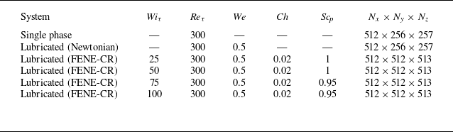

 Wiτ=50
 Wiτ=100

 a
 Wiτ
 z/h=−0.7
 b
 Qtot/QSP
 Qm/QSP
 Wiτ
 QSP
 Wiτ=0

 uτ2
 a
 [u′u′]
 b
 [v′v′]
 c
 [w′w′]
 d
 −[u′w′]
 z/h
 z/h=−0.7
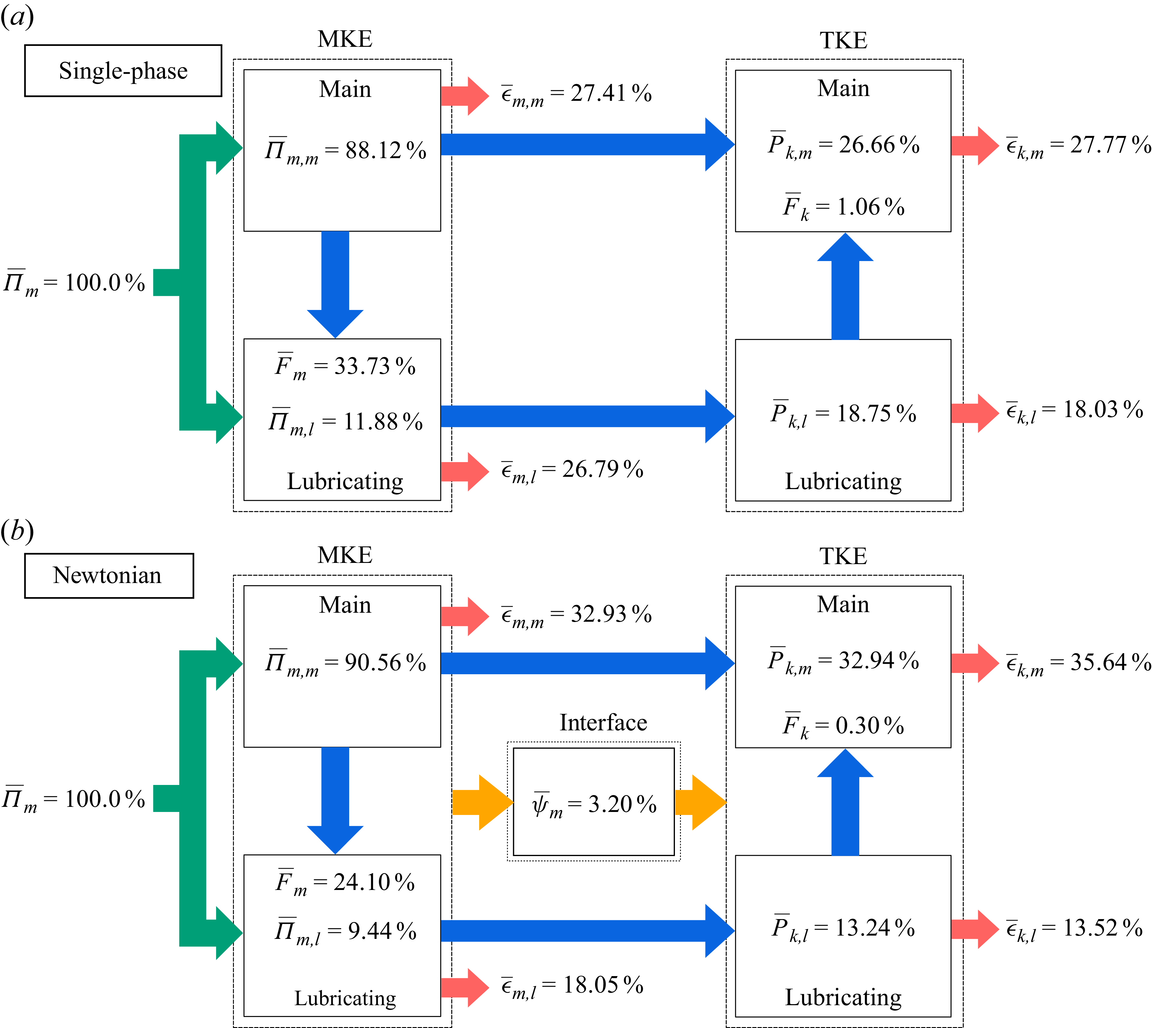
 a
 z/h=−0.7
 Π¯m
 ϵ¯m
 ϵ¯k
 P¯k
 b
 ψ¯m

 a
 Wiτ=25
 b
 Wiτ=50

 a
 Wiτ=75
 b
 Wiτ=100

 a
 Wiτ
 ψ¯m,N
 P¯k,l,N
 P¯pm,l
 P¯pk,l
 Π¯m,l,N
 b
 ζ/h
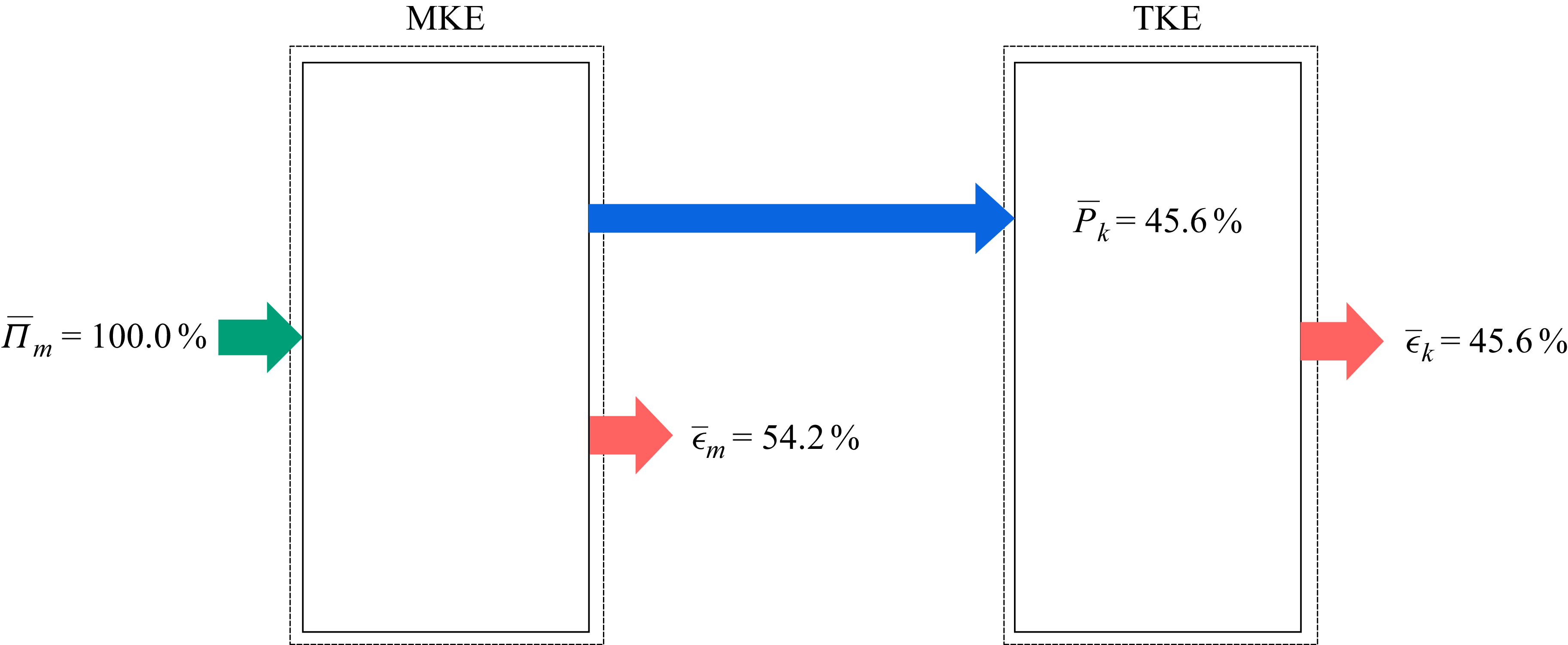

 a
 tr(C)¯/L2
 Wiτ
 τnn=(1−x0)τpxz¯/Reτ
 b
 tr(C)/L2
 z/h=−0.7
 z/h=−0.85

 Open access

