1. Introduction
Jets in crossflow have been extensively investigated due to the diversity of flows in which they find application and the complexity of the physics involved. Mahesh (Reference Mahesh2013) provides a recent review of applications and experimental and computational work on these flows. Areas of interest include turbulent mixing, film cooling of turbine blades, subsonic/supersonic combustion and propulsion, geophysical flows, pollutant dispersion and biological flows.
As presented by Mahesh (Reference Mahesh2013), the most commonly studied jet in the case of crossflow is the canonical round jet, transversely injected for single-phase incompressible and compressible flows. Flows involving heat transfer have been investigated, where the jet is heated for anti-icing applications (Albugues Reference Albugues2005; Duda Reference Duda2012) or cooled for film cooling (Harrington et al. Reference Harrington, McWaters, Bogard, Lemmon and Thole2001; Fawcett et al. Reference Fawcett, Wheeler, He and Taylor2013). Reacting and non-reacting liquid jets in gas crossflow have been investigated for their significance in various combustion applications (Sallam, Aalburn & Faeth Reference Sallam, Aalburn and Faeth2004; Abdilghanie, Frouzakis & Fischer Reference Abdilghanie, Frouzakis and Fischer2013). New insights into many of these flows are being made using modern experimental diagnostics (New, Lim & Luo Reference New, Lim and Luo2006) and computational capabilities (Ilak et al. Reference Ilak, Schlatter, Bagheri and Henningson2012). Of particular interest in these studies is flow stability and development of coherent phenomena as the precursor to turbulence transition.
Jets in crossflow involving phase transition or bubbly flows do not appear to have been investigated to date. Such flows are of interest in hydrodynamic test facilities and in the ejection of fluid from moving ships and submarines. The consequences of interest in these flows include undesirable viscous or nuclei/bubble-laden wakes, unsteady loads and vibration, metal erosion and acoustic signatures. Atmospheric air ingested by the boundary layer about surface ships may promote gaseous or vaporous cavitation, or undesirable bubbly flows about disturbances such as a transversely ejected liquid or gas jet. This is particularly the case for high-speed ships, where low cavitation numbers can occur. For submarines, ejected liquid jets near the surface or ejected gas jets whilst submerged are of interest. Jets in crossflow may also be used for mixing and artificial thickening of boundary layers in hydrodynamic test facilities (Brandner et al. Reference Brandner, Belle, Pearce and Holmes2012) where cavitation occurrence may be undesirable, for example in hydroacoustic testing. Of particular interest in these applications, as well as in the classical cases, is the influence of the wall boundary layer on the flow physics.
The present work was conceived to gain insight into the nucleation and development of vaporous cavitation about a jet in crossflow in the hydrodynamic context. To this end, the range of jet to freestream velocity ratios of interest are relatively low compared with classical studies. Conversely, the Reynolds numbers achieved within the variable-pressure water tunnel used for the present work are relatively high compared with the typical subsonic single-phase gas flows but comparable with those for typical supersonic studies. The jet diameter to boundary layer thickness ratio of about 1 in the present study is similar to that for many within the literature (Jovanovic Reference Jovanovic2006; Megerian et al. Reference Megerian, Davitian, Alves and Karagozian2007; Ilak et al. Reference Ilak, Schlatter, Bagheri and Henningson2012). The presence of bubbly and cavitating flows about a jet in crossflow provides the opportunity, through visualisation, to gain further insight into these complex flows and for comparison with existing and future experiments and computational predictions.
2. Experimental overview
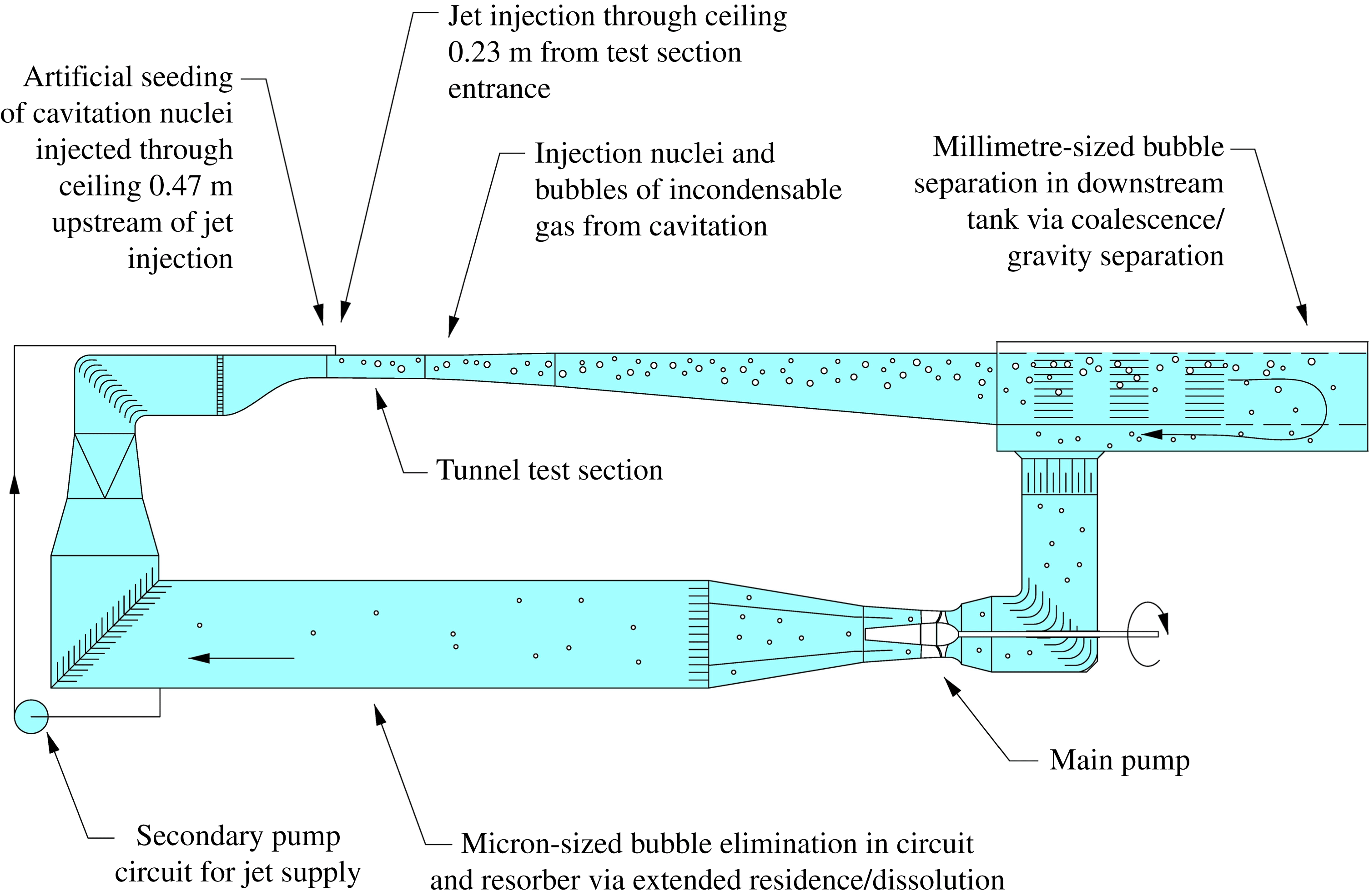
All experiments were carried out in the closed, recirculating variable-pressure water tunnel in the Cavitation Research Laboratory (CRL) at the University of Tasmania. Figure 1 shows a schematic of the tunnel circuit including the secondary circuit for jet supply. The tunnel test section is 0.6 m square by 2.6 m long, in which the operating velocity and pressure ranges are
 $2{-}12~\text{m}~\text{s}^{-1}$
and 4–400 kPa absolute, respectively. The tunnel volume is
 $365~\text{m}^{3}$
of demineralised water (conductivity of order
 $1~{\rm\mu}\text{S}~\text{cm}^{-1}$
). The tunnel has ancillary systems for rapid degassing and for continuous injection and removal of cavitation nuclei and large volumes of incondensable gas, as shown schematically in figure 1. The facility has also been designed for low vibration and background noise levels (Doolan et al.
Reference Doolan, Brandner, Butler, Pearce, Moreau and Brooks2013). Detailed descriptions of the facility are given in Brandner, Lecoffre & Walker (Reference Brandner, Lecoffre and Walker2006, Reference Brandner, Lecoffre and Walker2007).
Schematic of the water tunnel circuit and secondary pumping circuit for jet supply. The tunnel circuit is designed for continuous injection and separation of incondensable gas and cavitation nuclei via processes of coalescence/gravity separation of bubbles greater than about
 $100~{\rm\mu}\text{m}$
in a downstream tank and dissolution with extended residence in the lower limb or resorber. The jet fluid is extracted near the end of the resorber, ensuring it is nuclei free.

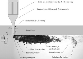
Schematic side view of jet in crossflow experimental setup. Shadow photograph of cavitation occurrence about the jet for
 $R=1.2$
,
 ${\it\sigma}_{\infty }=0.2$
and
 $\mathit{Re}_{J}=120\times 10^{3}$
. The scaled jet geometry and upstream boundary layer velocity profile are superimposed on the shadow photograph. Typical regions are shown that were sampled using high-speed photography for frequency measurement of coherent structures.

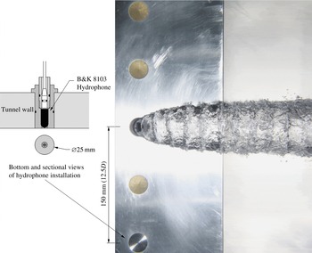
Photograph of the jet in crossflow from beneath for
 $R=1.0$
,
 ${\it\sigma}_{\infty }=0.1$
and
 $\mathit{Re}_{J}=100\times 10^{3}$
. The relative location of the hydrophone used for acoustic detection of cavitation inception is indicated, as well as sectional and plan-view drawings of its installation.

The transverse jet is supplied via a pump and secondary circuit with water extracted from the tunnel return limb, as shown in figure 1. The location of the water extraction is downstream of the tunnel sections for bubble separation and dissolution such that the injected fluid is expected to be nuclei free, as discussed in detail below. Figure 2 shows a schematic of the scaled jet geometry and upstream boundary layer velocity profile superimposed on a shadow photograph of cavitation occurrence about the jet with salient flow features noted. The 12 mm diameter transverse jet is injected via a flush nozzle, upstream of which is a contraction and a honeycomb. The parallel length of nozzle downstream of the contraction, required to penetrate the tunnel wall, is 4.25 diameters long. The contraction has an area ratio of 17.36 and is 4.5 diameters long. The contraction has a fifth-order polynomial profile with zero first and second derivatives at exit. The honeycomb of
 $50~{\rm\mu}\text{m}$
aluminium has 6 mm hex cells and is 10 cell dimensions long. The jet is located on the centreline of the test section ceiling 0.23 m downstream from the test section entrance. The jet velocity is determined from the contraction pressure differential calibrated for the Reynolds number range used. Figure 3 shows an installation schematic and the relative location of the hydrophone used for acoustic detection of cavitation inception.
All tests were carried out at a fixed freestream Reynolds number which may be based on either the tunnel cross-section dimension,
 $\mathit{Re}_{H}=U_{\infty }H/{\it\nu}=5\times 10^{6}$
, or the jet diameter,
 $\mathit{Re}_{D}=U_{\infty }D/{\it\nu}=10^{5}$
, where the tunnel cross-sectional dimension
 $H$
is
 $0.6~\text{m}$
and the jet diameter
 $D$
is
 $0.012~\text{m}$
,
 $U_{\infty }$
is the freestream velocity and
 ${\it\nu}$
is the kinematic viscosity. The jet velocity ratio,
 $R=U_{J}/U_{\infty }$
, was varied between 0.2 and 1.6, where
 $U_{J}$
is the mean jet velocity. This corresponds to a range of jet-velocity-based Reynolds numbers,
 $\mathit{Re}_{J}=U_{J}D/{\it\nu}$
, ranging from about
 $25\times 10^{3}$
to
 $160\times 10^{3}$
. The freestream cavitation number was varied from inception values of up to about 10, down to a minimum of 0.1. The freestream cavitation number is defined as
 ${\it\sigma}_{\infty }=(p_{\infty }-p_{v})/(0.5{\it\rho}U_{\infty }^{2})$
, where
 $p_{\infty }$
is the absolute static pressure at the test section ceiling,
 $p_{v}$
the vapour pressure and
 ${\it\rho}$
is the fluid density. A jet-velocity-based cavitation number,
 ${\it\sigma}_{J}=(p_{\infty }-p_{v})/(0.5{\it\rho}U_{J}^{2})=({\it\sigma}_{\infty })/R^{2}$
, may also be defined as typically used for quantifying inception about open jets (submerged in a quiescent environment).
The water tunnel velocity and pressure are regulated in real time to maintain the set
 $\mathit{Re}_{H}$
and
 ${\it\sigma}_{\infty }$
values using closed-loop feedback control. The velocity of the injected jet is likewise regulated to maintain the set
 $R$
value. The water temperature is measured in real time, and the fluid physical properties are calculated from it for control of the non-dimensional parameters.
Cavitation inception was investigated for practically achievable bounding cases of high and low susceptibility to phase change, that is, either where the upstream boundary layer was artificially seeded with high concentrations of relatively large nuclei or where the boundary layer was deplete of cavitation nuclei.
The high-susceptibility case is achieved using artificial seeding of nuclei introduced into the boundary layer via a flush 1 mm diameter port at a location 0.47 m upstream of the jet axis. The microbubble generator used for the present work and its operation is described in Brandner et al. (Reference Brandner, Wright, Pearce, Goldsworthy and Walker2010b
). The generator was operated to produce microbubbles in a size range of
 $10{-}200~{\rm\mu}\text{m}$
with a dominant size of about
 $25~{\rm\mu}\text{m}$
diameter, at a rate of about 400 kHz. Based on estimated production rate and the observed dispersion (figure 11), the estimated nuclei sizes and concentrations (
 ${>}100~\text{cm}^{-3}$
) are of the order that essentially no static delay of inception below vapour pressure would occur (Franc & Michel Reference Franc and Michel2004). On this basis, the flow is saturated such that variations in nuclei content have little effect on inception (Frechou et al.
Reference Frechou, Dugue, Briancon-Marjollet, Fournier, Darquier, Descotte and Merle2001).
The nuclei deplete case is achieved in the CRL water tunnel as the circuit architecture has sections designed for elimination of nuclei or so-called free gas (via gravity separation and dissolution) provided the dissolved gas content is sufficiently low. Design studies and previous work reported from facilities using the same operational principles as the CRL tunnel have shown that for elimination of free gas the dissolved gas concentration is required to be less than about 30 % of saturation at atmospheric pressure (Frechou et al.
Reference Frechou, Dugue, Briancon-Marjollet, Fournier, Darquier, Descotte and Merle2001). For the present work the dissolved oxygen concentration was maintained at about 3 p.p.m. for all test cases. The saturated dissolved oxygen concentration at standard conditions for temperature and pressure is about 10 p.p.m. (Sander Reference Sander1999). This condition practically achieves low susceptibility with studies by Gindroz & Billet (Reference Gindroz and Billet1998) reporting tensions measured with a venturi-type cavitation susceptibility meter corresponding to nuclei sizes of order
 $1~{\rm\mu}\text{m}$
diameter. For the present work, assuming no static delay of inception below vapour pressure for the seeded cases, the inception values for the unseeded cases give similar results to those of Gindroz & Billet (Reference Gindroz and Billet1998) with corresponding nuclei sizes less than
 $1~{\rm\mu}\text{m}$
radius.
The dynamic or intermittent nature of cavitation inception was acoustically detected using a hydrophone held in a flooded volume behind a plate flush with the tunnel ceiling perforated with an array of 1 mm diameter holes, as shown in figure 3. The hydrophone is located at the same streamwise position as the jet offset 150 mm from the test section centreplane. The hydrophone used was a B&K model 8103, conditioned using a B&K NEXUS model 2692-I04 charge amplifier. All acoustic records were for a 60 s sample period at 100 kHz using a National Instruments NI PXIe 4493 data acquisition card.
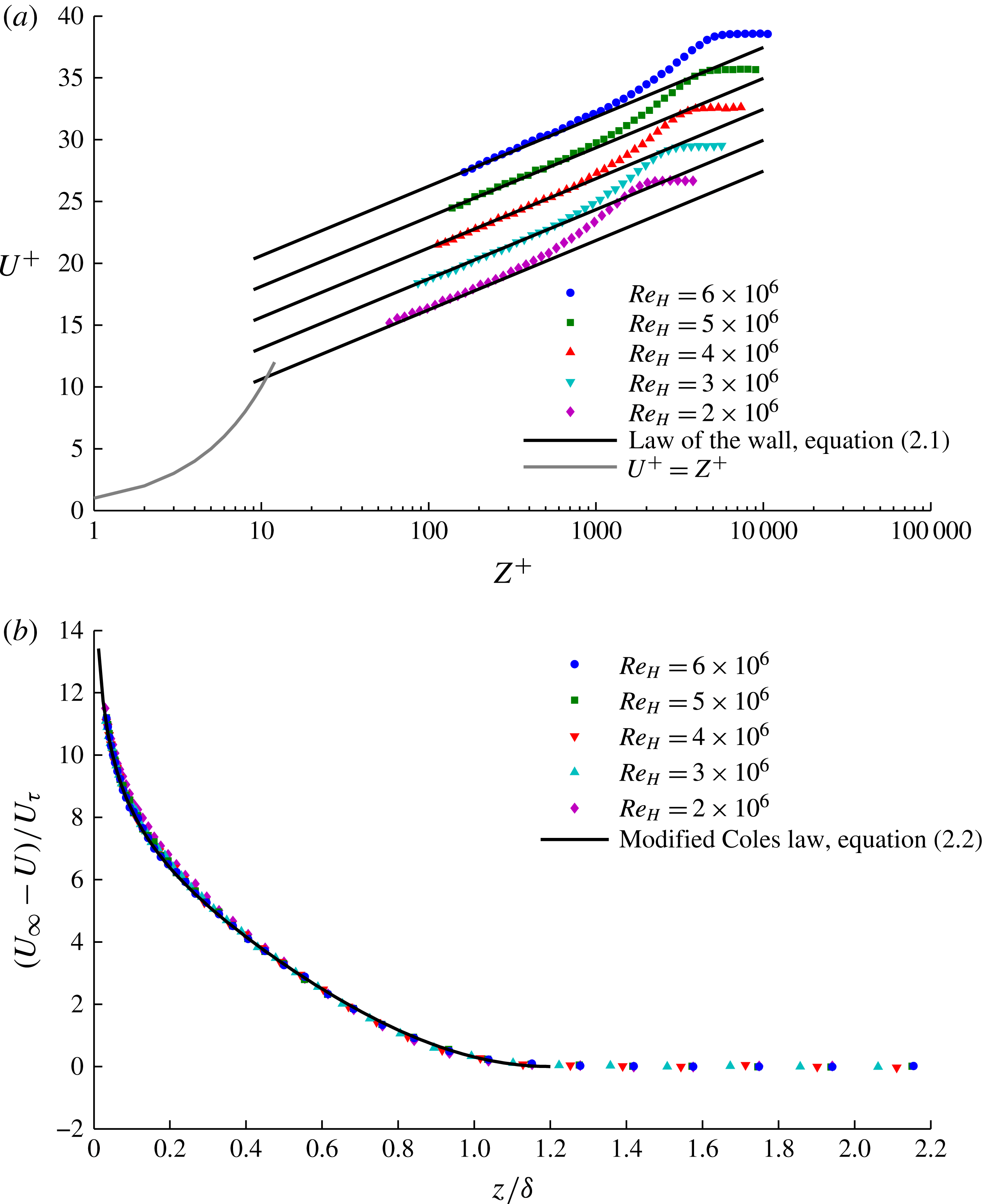
Test section ceiling undisturbed boundary layer velocity profiles, measured at the jet location for a range of
 $\mathit{Re}_{H}$
values scaled using inner and outer variables, are shown in figure 4. These were measured using a 0.7 mm outside, by 0.4 mm inside, diameter total head tube. Total pressures were measured relative to a wall-static tapping via a multiplexing valve, enabling the pressure transducer zero to be updated at every measurement. Measured pressures were normalised for small temporal variations of freestream velocity using the tunnel contraction differential that was simultaneously acquired, as well as being normalised on the freestream measurement. By this method the pressure transducer zero and span errors are eliminated, as well as changes due to any freestream temporal variations. Boundary layer traverses were made by automated traverse consisting of 40 points on a log distribution. Acquisition durations for each point corresponded to a minimum of 5000 boundary layer turnovers,
 $TU_{\infty }/{\it\delta}$
, where
 $T$
is the acquisition time and
 ${\it\delta}$
is the boundary layer thickness at which
 $U=0.99U_{\infty }$
. This number of turnovers has been found to provide converged velocity measurements. Further details of the measurement techniques used are described in Brandner et al. (Reference Brandner, Belle, Pearce and Holmes2012).
Tunnel ceiling undisturbed boundary layer profiles at the jet injection location as a function of tunnel Reynolds number
 $\mathit{Re}_{H}$
, scaled using (a) inner variables (2.1) and (b) outer variables (2.2). The profiles are independent of
 $\mathit{Re}_{H}$
for all but the lowest value.

The law of the wall is given by
 $$\begin{eqnarray}U^{+}=\frac{1}{{\it\kappa}}\ln z^{+}+B,\end{eqnarray}$$
where
 $U^{+}=U/U_{{\it\tau}}$
,
 $U$
is the local velocity,
 $U_{{\it\tau}}$
is the wall friction velocity,
 $z^{+}=zU^{+}/{\it\nu}$
,
 ${\it\nu}$
is the kinematic viscosity,
 ${\it\kappa}$
is the von Kármán constant, 0.41, and
 $B$
is an additive constant taken as 5.0.
A modified Coles law of the wake is given by
 $$\begin{eqnarray}\frac{U_{\infty }-U}{U_{{\it\tau}}}=-\frac{1}{{\it\kappa}}\left(\ln {\it\eta}-2{\it\Pi}\cos ^{2}\frac{{\rm\pi}{\it\eta}}{2}+\frac{1-{\it\eta}^{3}}{3}\right);\end{eqnarray}$$
where
 ${\it\eta}=z/{\it\delta}_{c}$
,
 ${\it\delta}_{c}$
is the boundary layer thickness at which
 $U=U_{\infty }$
and
 ${\it\Pi}$
is the wake strength factor taken as 0.62. This formulation of the modified Coles law is by Guo, Julien & Meroney (Reference Guo, Julien and Meroney2005), although that by Jones, Marusic & Perry (Reference Jones, Marusic and Perry2001) provides a similar fit. Test section boundary layers were found to have
 ${\it\delta}_{c}=1.2{\it\delta}$
(to within 1 %) for all streamwise locations and
 $\mathit{Re}_{H}$
values (Brandner et al.
Reference Brandner, Belle, Pearce and Holmes2012). The profiles are virtually independent of
 $\mathit{Re}_{H}$
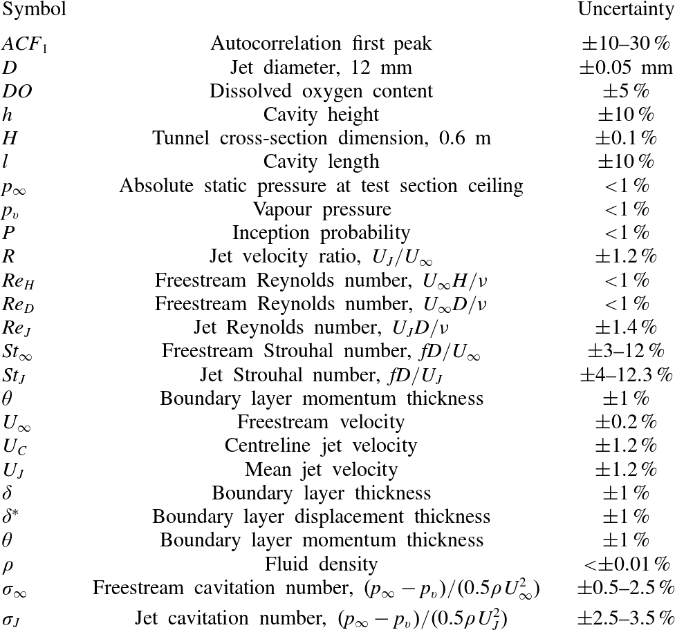
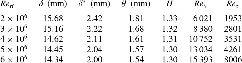
for all but the lowest values. Table 1 provides a list of parameters with estimated uncertainties. Table 2 lists the variation of boundary layer properties with
 $\mathit{Re}_{H}$
. For the present work at
 $\mathit{Re}_{H}=5\times 10^{6}$
, the ratio
 ${\it\delta}/D=1.18$
.
List of parameters and estimated uncertainties.

Boundary layer properties.
 ${\it\delta}$
is the boundary layer thickness at which
 $U=0.99U_{\infty }$
,
 ${\it\delta}^{\ast }$
is the displacement thickness,
 ${\it\theta}$
is the momentum thickness,
 $H={\it\delta}^{\ast }/{\it\theta}$
is the boundary layer shape factor and
 $\mathit{Re}_{{\it\theta}}=U_{\infty }{\it\theta}/{\it\nu}$
and
 $\mathit{Re}_{{\it\tau}}=U_{{\it\tau}}{\it\delta}/{\it\nu}$
are Reynolds numbers based on the momentum thickness and wall friction velocity, respectively.

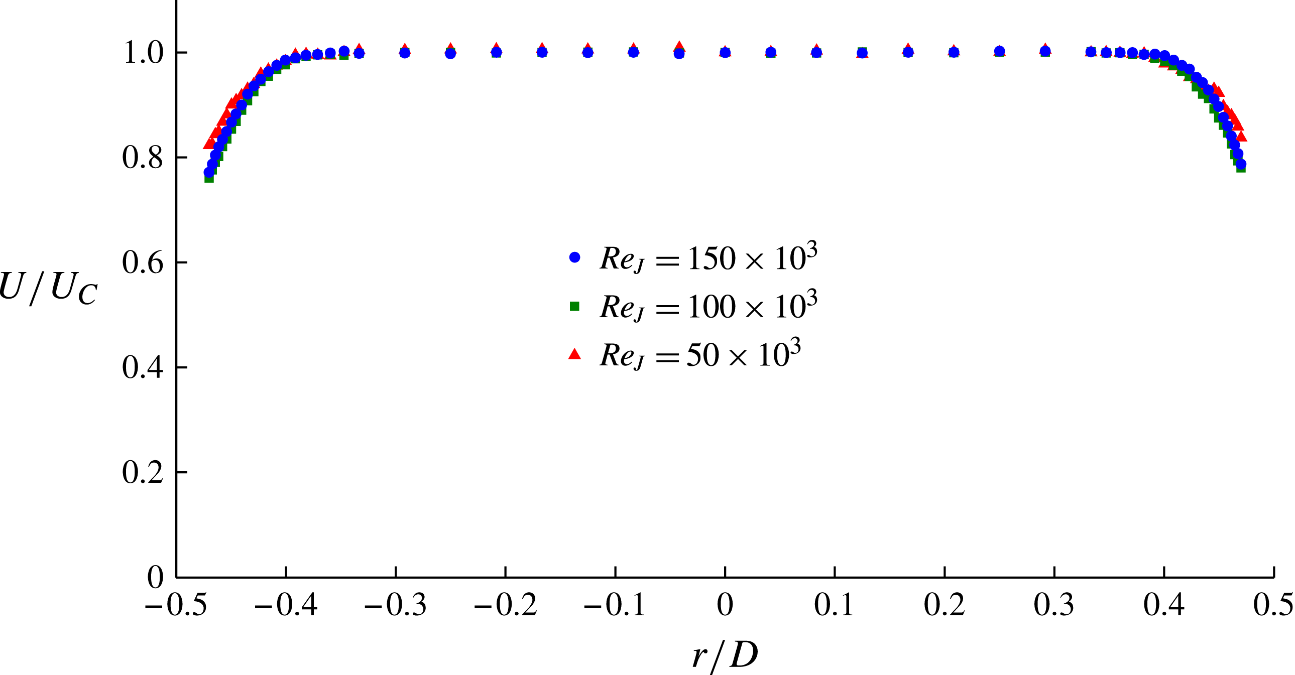
Figure 5 shows the velocity profiles,
 $U/U_{C}$
, of the exiting jet, for several
 $\mathit{Re}_{J}$
values, measured for
 $R=\infty$
using the same total head tube size and similar techniques to the boundary layer profiles described above.
 $U$
is the local jet velocity at radius
 $r$
, and
 $U_{C}$
is the centreline jet velocity. The profiles are independent of
 $\mathit{Re}_{J}$
for values at most greater than 100 000. They are uniform except for boundary layers of about
 $0.125D$
thickness that develop due to the short length of parallel nozzle downstream of the contraction.
Velocity profiles,
 $U/U_{C}$
, of the exiting jet for
 $R=\infty$
showing the independence of
 $\mathit{Re}_{J}$
for values at most greater than 100 000. The profiles are uniform but for boundary layers of about
 $0.125D$
thickness that develop due to the short length of parallel nozzle downstream of the contraction.
 $U$
is the local jet velocity at radius
 $r$
, and
 $U_{C}$
is the centreline velocity.

Still and high-speed photography were used to investigate the macroscopic cavitation phenomena that developed after inception with reduction of the cavitation number. Still photography was obtained using a Canon EOS 50D 35 mm digital SLR camera (image resolution
 $4752~\text{pixel}\times 3168~\text{pixel}$
) with a Canon EF 24–70 mm lens. The cavitation was forward- and back-lit using triggered stroboscopic lighting (DRELLO 1018/LE4040). The back-lighting was diffused using a 3 mm white acrylic sheet. High-speed photography was carried out using a LaVision HighSpeedStar5 camera with a Nikkor 55 mm
 $f/1.4$
or a Nikkor 24 mm
 $f/2.8$
lens, depending on magnification. The camera was operated at a frame rate of 6 kHz with a resolution of
 $1024~\text{pixel}\times 512~\text{pixel}$
and controlled using DaVis 7.2.2 software. The cavitation was back-lit using a Dedolight DLH650 diffused similarly through a 3 mm white acrylic sheet.
From the high-speed photography, cavity dynamics were analysed using time series of spatially averaged pixel intensities from regions of interest (figure 2), similar to the methods used in Brandner et al. (Reference Brandner, Walker, Niekamp and Anderson2010a ). The time series data obtained were examined using both direct event counting and the continuous wavelet analysis method of Torrence & Compo (Reference Torrence and Compo1998) to obtain the shedding frequencies. The Morlet-6 wavelet was used to obtain the frequencies, and the Derivative of Gaussian-2, (DOG-2) wavelet was used to identify the individual shedding events.
3. Results
3.1. Cavitation inception
Cavitation inception is a complex multidisciplinary phenomenon that remains a fundamental aspect of general cavitation research. Classical reviews on inception in hydrodynamic flows by Acosta & Parkin (Reference Acosta and Parkin1975) and Rood (Reference Rood1991), for example, discuss the role of surface topography, freestream nuclei and flow physics. More recently, Joseph (Reference Joseph1998) provided a theoretical criterion for inception based on the state of stress within a flowing liquid, and in particular for the case of shear flows relevant to the present work. Furukawa & Tanaka (Reference Furukawa and Tanaka2006) present a more fundamental criterion for flow-induced instability such as cavitation inception for fluids whose viscosity is density-dependent (although water is not one of these fluids).
The definition of cavitation inception depends on the nature of the cavitation under investigation. For unsteady or dynamic cavitation this requires a definition consistent with the inception process, from the first signs of activated nuclei through to established macroscopic cavities. Previous work on cavitation inception in open jets has used the rates of cavitation events from surface pressure, acceleration or acoustic measurements to quantify or define the inception process (e.g. Ooi Reference Ooi1985; Pauchet, Retailleau & Woillez Reference Pauchet, Retailleau and Woillez1992; Gopalan, Katz & Knio Reference Gopalan, Katz and Knio1999; Straka et al. Reference Straka, Meyer, Fontaine and Welz2010).
For the present work inception for the unseeded case was observed to be a process of an intermittent nature starting with infrequent audible events increasing in occurrence or duration with reduction in
 ${\it\sigma}_{\infty }$
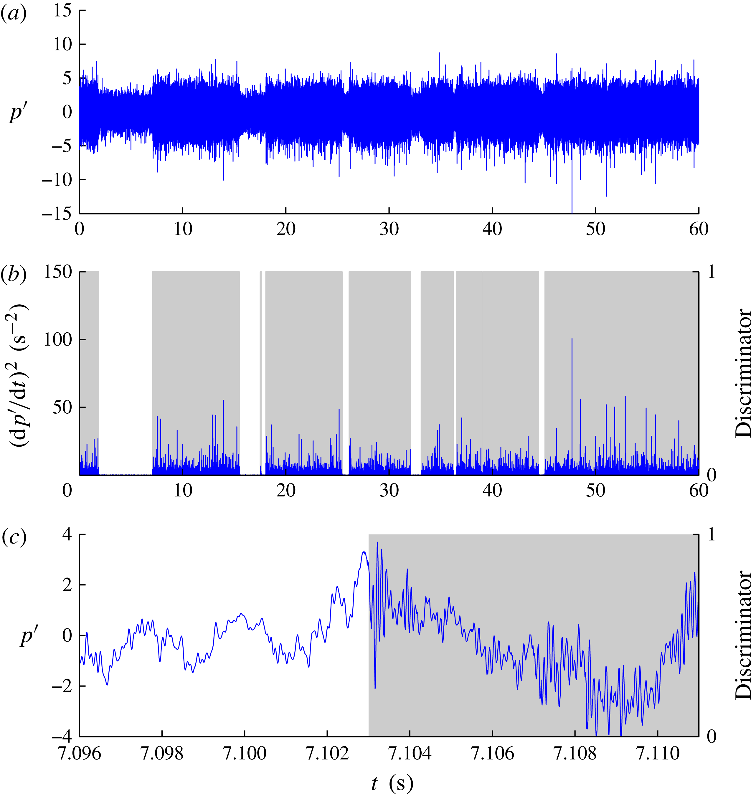
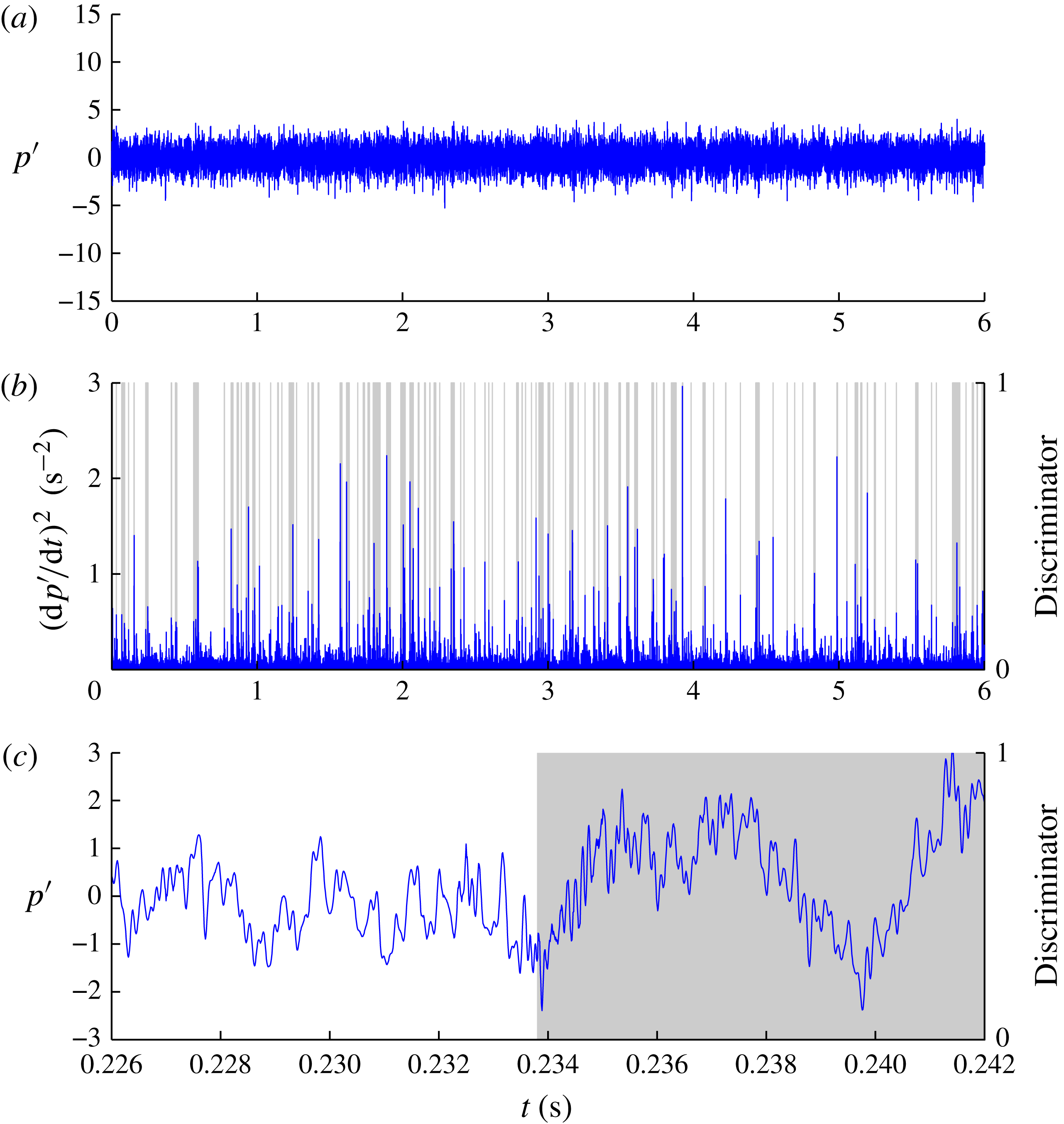
. An acoustic method, as described in the previous section, was therefore chosen for inception detection. Figure 6(a) shows a 60 s acoustic record for the unseeded case, showing clearly defined periods when no cavitation occurs (background turbulent noise level) and periods of increased noise level where cavitation occurs. The measured sound pressure is normalised,
 $p^{\prime }$
, using the root mean square of the background noise (without cavitation). To quantify the duration for which cavitation was present, an intermittency approach similar to those used for turbulence intermittency was chosen. Using this method it is possible to quantify the inception process from no cavitation (0 % probability) through to where cavitation was constantly present (100 % probability). The peak–valley counting technique developed for turbulence intermittency, as implemented by Clarke, Brandner & Walker (Reference Clarke, Brandner and Walker2008), was used to discriminate between periods with or without cavitation.
(a) Time series of normalised hydrophone output,
 $p^{\prime }$
, for
 $R=1.0$
and
 ${\it\sigma}_{\infty }=1.67$
(without nuclei seeding) showing periods with and without cavitation. (b) Time series of output from algorithm used for detection and discrimination of cavitation inception and hence probability; for this case
 $P=83\,\%$
. (c) Short time segment of the hydrophone output for a period without and with cavitation. The frequency of the excited cavitation bubbles is about 10 kHz.

For the seeded case, where there is an abundance of nuclei, the inception process involved more frequent events but with lower acoustic amplitudes than the unseeded case. Figure 7 shows a 6 s acoustic record for the seeded case. In both cases records were made for 60 s but for the seeded case only a 6 s segment is shown, to demonstrate the much greater frequency of cavitation events compared with the unseeded case. For the seeded case the frequency and amplitude of the events increased with reduction in
 ${\it\sigma}_{\infty }$
as increasing numbers of progressively smaller nuclei were activated. Therefore the intermittency approach could also be used to quantify the inception process for the seeded case, from where few events were detected through to where there is continuous cavitation noise. By using the same algorithm to quantify inception in both cases, comparison can be made of these two bounding cases of high and low susceptibility to phase change over the range of
 $R$
values investigated.
(a) Time series of normalised hydrophone output,
 $p^{\prime }$
, for
 $R=1.0$
and
 ${\it\sigma}_{\infty }=8.6$
(with artificial nuclei seeding) showing periods with and without cavitation. (b) Time series of output from algorithm used for detection and discrimination of cavitation inception and hence probability; for this case
 $P=18\,\%$
. Only a 6 s sample (of a total 60 s) is shown here due to the higher frequency of cavitation events for the seeded case as opposed to the unseeded case, shown in figure 6, where the full 60 s sample was shown due to the lower frequency but longer duration events. (c) Short time segment of the hydrophone output for a period without and with cavitation. The frequency of the excited cavitation bubbles is about 8.5 kHz.

The technique implemented uses the square of the time derivative of the hydrophone output as the detector function. A discrimination algorithm is used to determine whether a peak or valley has occurred if the local maxima or minima exceed a threshold value. If another peak or valley occurs within a time window the discriminator is maintained at 1 or is otherwise reset to 0. The threshold value and window length were determined experimentally to give intermittency or probability of cavitation inception,
 $P$
, varying between 0 and 100 % with reduction of
 ${\it\sigma}_{\infty }$
, for the cases with and without nuclei seeding. For the unseeded case the threshold and window were set at
 $6~\text{Pa}^{2}~\text{s}^{-2}$
(or
 $(\text{d}p^{\prime }/\text{d}t)^{2}=37.94~\text{s}^{-2}$
) and 50 ms respectively, and for the seeded case
 $6~\text{Pa}^{2}~\text{s}^{-2}$
(or
 $(\text{d}p^{\prime }/\text{d}t)^{2}=39.26~\text{s}^{-2}$
) and 20 ms respectively. The threshold value was set the same for both cases, but the window length was set shorter for the seeded case due to the greater frequency of individual cavitation events or nuclei activations. It was found that a window length of 20 ms provided the same results for most
 $R$
values for the unseeded case except for
 $R=0.5$
, where values of 0 and 100 % were not achieved.
Sample results from the intermittency analysis are shown in figures 6 and 7 for the unseeded and seeded cases respectively. These figures show the acoustic record and cavitation detection over characteristic durations, as described above, and sample short time segments of acoustic records spanning the transition between no cavitation and cavitation. Figure 6, the unseeded case, is for
 $R=1.0$
and
 ${\it\sigma}_{\infty }=1.67$
, for which
 $P=83\,\%$
, and figure 7, the case with nuclei seeding, for
 $R=1.0$
and
 ${\it\sigma}_{\infty }=8.6$
, for which
 $P=18\,\%$
.
Of interest is the reduced noise level for the seeded cases compared with the unseeded cases for all
 $P$
values. At
 $P=100\,\%$
for
 $R=1.0$
, for the seeded case the normalised root mean square of the hydrophone output is 0.49 compared with 0.52 for the unseeded case. For small
 $P$
values (
 ${<}$
5 %) for
 $R=1.0$
, the normalised root mean square of the seeded case is about 0.38 compared with the unseeded case of 0.41. Fuster, Pham & Zaleski (Reference Fuster, Pham and Zaleski2014) provide a theoretical/numerical basis for this phenomenon and show that there is a critical void fraction or air concentration beyond which the dynamic response of the system is attenuated and radiated sound is damped. They also note that the concentration threshold requires only small amounts of air as experimentally observed by Reisman, Duttweiler & Brennen (Reference Reisman, Duttweiler and Brennen1997), who showed large reductions of noise from cloud cavitation about a hydrofoil with air injection into the cavitating region.
Inception for the unseeded cases typically occurred at low
 ${\it\sigma}_{\infty }$
values, compared with the seeded cases, these being required to activate the few high-strength nuclei present. As noted in the previous section, estimated nuclei sizes for the unseeded case are less than
 $1~{\rm\mu}\text{m}$
radius. Due to these low
 ${\it\sigma}_{\infty }$
values, the cavities once activated tended to remain present, producing noise for a relatively longer duration, compared with the seeded cases, before their collapse or condensation. The additional frequency ever-present with the onset of cavitation shown in figure 6(c) is about 10 kHz.
For the seeded case inception typically occurs at high
 ${\it\sigma}_{\infty }$
values due to the large nuclei present estimated to be of order
 $100~{\rm\mu}\text{m}$
radius. Due to the abundance of nuclei over a range of sizes the much more frequent but short duration noise events detected are attributable to excitation or growth/collapse cycles of individual nuclei rather than the noise produced by a sustained cavity as for the unseeded case. The additional frequency ever-present with the onset of cavitation shown in figure 7(c) is slightly less than the unseeded case, about 8.5 kHz, implying larger cavity volumes reflecting the much larger nuclei sizes present in the seeded case.
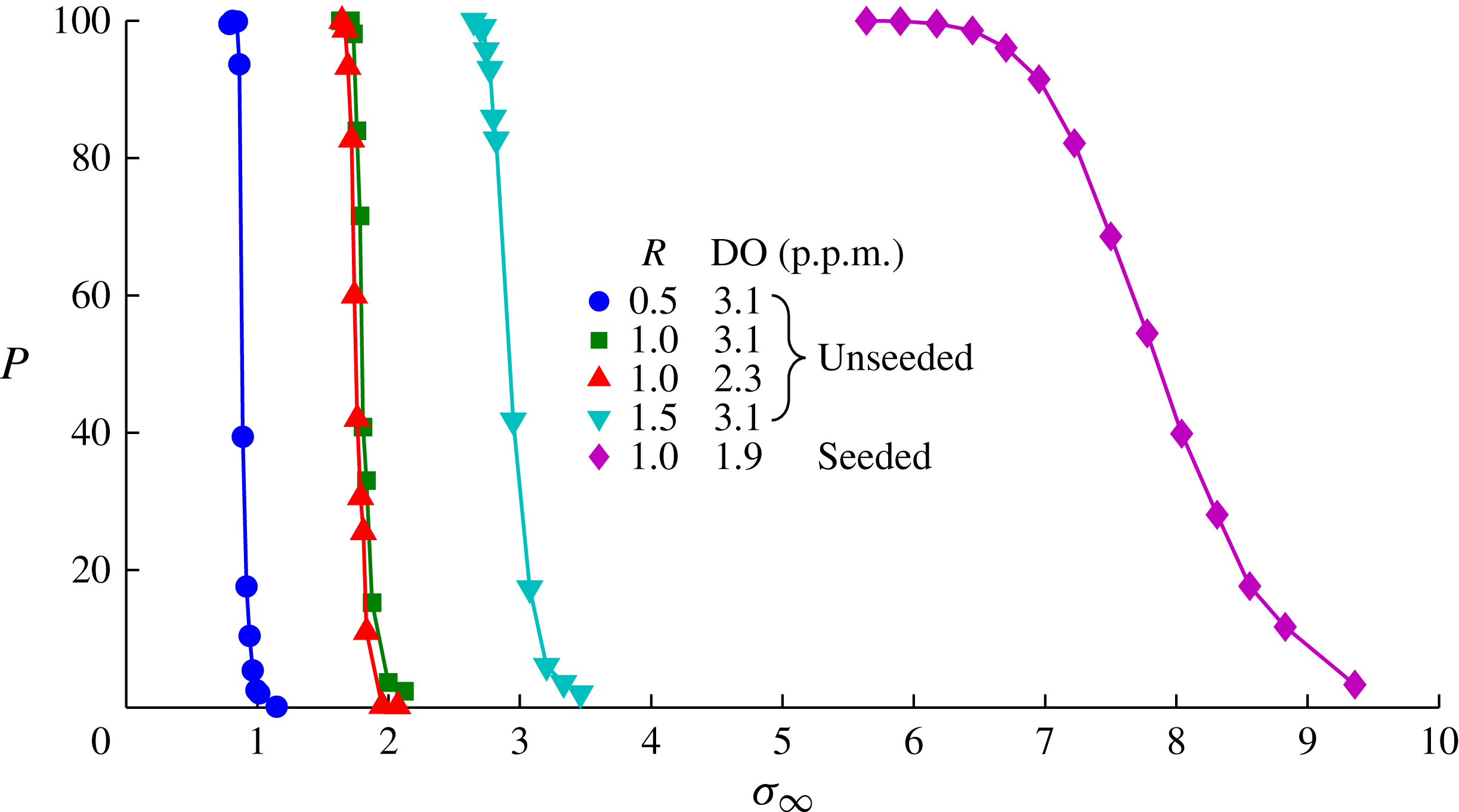
Figure 8 shows
 $P$
as a function of
 ${\it\sigma}_{\infty }$
for
 $R=0.5$
, 1.0 and 1.5 for the unseeded case and
 $R=1.0$
for the seeded case. Comparison of the curves for
 $R=1.0$
shows the large differences between incipient cavitation numbers due to the differences in size and concentration of nuclei between the unseeded and seeded cases. For the seeded case, the inception process starts at a high
 ${\it\sigma}_{\infty }$
value and progresses through to
 $P=100\,\%$
over a large
 ${\it\sigma}_{\infty }$
range as progressively more nuclei are activated with reduction of
 ${\it\sigma}_{\infty }$
. For the unseeded case where the flow is nuclei deplete, the inception progresses from
 $P=0$
to 100 % over a small
 ${\it\sigma}_{\infty }$
range due to a much more limited range of nuclei sizes or strengths. Incipient cavitation numbers are increased with increase in
 $R$
due to the higher velocity gradients and consequent reduction of minimum pressure with increase in jet speed relative to the freestream. Two curves for
 $R=1.0$
with different dissolved gas contents are shown to demonstrate the small effect dissolved gas has on inception at a low level of saturation.
Probability of cavitation inception by acoustic detection as a function of
 $R$
and
 ${\it\sigma}_{\infty }$
with and without artificial seeding of nuclei. Inception for the seeded case occurs at higher
 ${\it\sigma}_{\infty }$
values, and over a larger range, compared with the unseeded case, due to the greater number and size of nuclei which are progressively activated with reduction in
 ${\it\sigma}_{\infty }$
. For the unseeded or nuclei deplete case, nuclei are of order
 $1~{\rm\mu}\text{m}$
diameter, and for the seeded case there is a high concentration (
 ${>}100~\text{cm}^{-3}$
) of large nuclei of diameter range
 $10{-}200~{\rm\mu}\text{m}$
.

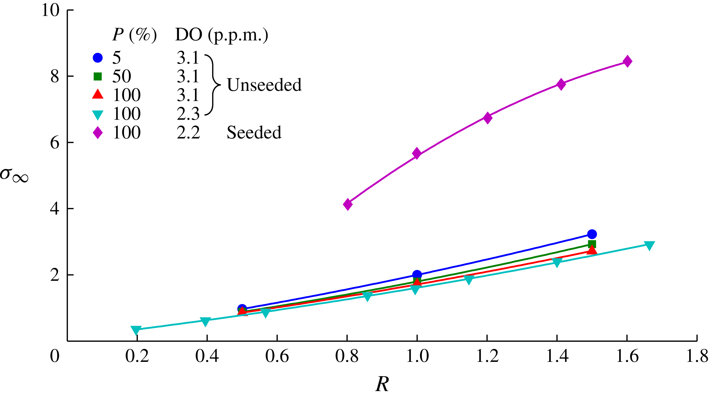
Figure 9 shows contours of
 $P$
for 5 %, 50 % and 100 % for the unseeded cases and 100 % for the seeded case as a function of
 $R$
. A second contour of
 $P=100\,\%$
, for a greater
 $R$
range, for the unseeded case with dissolved
 $\text{O}_{2}$
content of 2.3 p.p.m. is also shown. This second curve again shows the relatively small effect dissolved gas content has at a low level of saturation. The curves for
 $P=100\,\%$
, for both the unseeded and seeded cases, show slightly nonlinear dependence on
 $R$
. For the seeded case there is a more nonlinear dependence of inception probability on
 $R$
, with the curve tending towards the unseeded case at the lower
 $R$
values tested. It was found that below
 $R=0.8$
for the seeded cases the signal-to-noise ratio of the nuclei activations compared with background turbulent noise became too small for reliable use of the intermittency approach to quantify the probability of inception.
Contours of probability of cavitation inception as a function of
 $R$
and
 ${\it\sigma}_{\infty }$
with and without artificial seeding of nuclei, showing the large difference between the two cases. Two curves for different dissolved gas contents for
 $P=100\,\%$
for the unseeded case are shown to demonstrate the relatively small effect dissolved gas content has at this level of saturation. For the unseeded or nuclei deplete case, nuclei are of order
 $1~{\rm\mu}\text{m}$
diameter, and for the seeded case there is a high concentration (
 ${>}100~\text{cm}^{-3}$
) of large nuclei of diameter range
 $10{-}200~{\rm\mu}\text{m}$
.

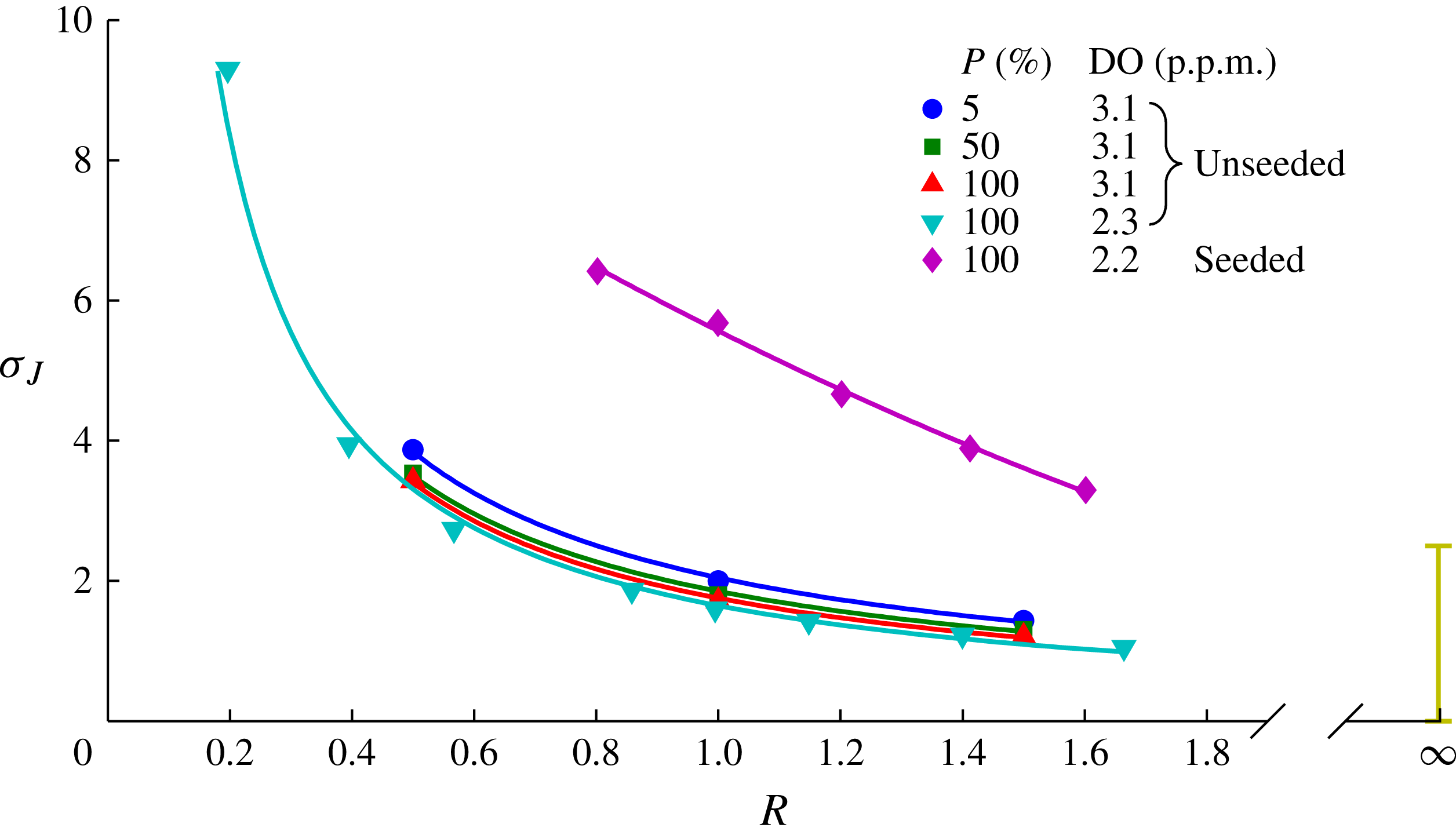
As noted above, inception for open jets (
 $R=\infty$
) is often based on cavitation event rates using a jet-velocity-based cavitation number,
 ${\it\sigma}_{J}={\it\sigma}_{\infty }/R^{2}$
, as defined earlier. Despite the differences in the nature of inception between the cases of a jet in crossflow and open jets, it is of interest to compare the incipient cavitation numbers. To make this comparison the results presented in figure 9 are replotted in figure 10 using a jet-based cavitation number, and typical ranges of incipient cavitation numbers for open jets reported in the literature are shown. The range of open jet data shown is from Ooi (Reference Ooi1985), Pauchet et al. (Reference Pauchet, Retailleau and Woillez1992), Gopalan et al. (Reference Gopalan, Katz and Knio1999) and Straka et al. (Reference Straka, Meyer, Fontaine and Welz2010). The jet in crossflow curve for the seeded case shows a near-linear dependence on
 $R$
whereas the curves for the unseeded cases show a power-law dependence on
 $R$
(for the
 $P=100\,\%$
curve
 ${\it\sigma}_{\infty }=1.65R^{-1}$
). For both unseeded and seeded cases the curves tend toward the range of data obtained for the open jets.
Incipient cavitation numbers (based on jet velocity) for the present jet in crossflow compared with the typical range of values (bar at
 $R=\infty$
) for open jets reported in Ooi (Reference Ooi1985), Pauchet et al. (Reference Pauchet, Retailleau and Woillez1992), Gopalan et al. (Reference Gopalan, Katz and Knio1999) and Straka et al. (Reference Straka, Meyer, Fontaine and Welz2010). For the unseeded or nuclei deplete case, nuclei are of order
 $1~{\rm\mu}\text{m}$
diameter, and for the seeded case there is a high concentration (
 ${>}100~\text{cm}^{-3}$
) of large nuclei of diameter range
 $10{-}200~{\rm\mu}\text{m}$
.

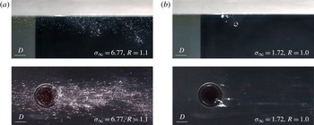
Figure 11 shows typical images from photography of the jet from the side and below, taken sequentially, at nominally
 $R=1.0$
and
 $P=100\,\%$
, for the unseeded and seeded cases. The unseeded images show that inception is localised and occurs either side just downstream of the exiting jet in regions of high shear and initial vortex formation (as further revealed with reduction of
 ${\it\sigma}_{\infty }$
discussed below). These cavities are transient but ever-present for
 $P=100\,\%$
. For the seeded case, a much greater nuclei (or microbubble) concentration downstream of the jet is evident in both the side and bottom images associated with the more frequent and distributed, but weaker, nuclei activations.
Photographs of incipient cavitation, from the side and below, (a) with and (b) without artificial seeding of the upstream boundary layer with cavitation nuclei. For the unseeded case at
 $P=100\,\%$
localised transient cavities occur either side of the exiting jet. In the seeded case the larger microbubble concentrations downstream of the jet exit show the more distributed and frequent, but weaker, nuclei activations.

As noted in § 2, the jet velocity profiles at exit, for
 $R=\infty$
, show that boundary layers of about
 $0.125D$
develop due to the short nozzle length downstream of the contraction. The fact that inception occurs about the exiting jet in these regions of high shear suggests that the jet exit profile may influence the incipient cavitation number.
As noted above, the intermittent nature of inception for the jet in crossflow is in contrast with the inception process for open jets where it is quantified by rates of individual events. Inception in open jets occurs within vortex cores forming in the developing shear layers (Gopalan et al. Reference Gopalan, Katz and Knio1999). For the jet in crossflow regions of high shear, separation and reversed flow occur downstream of the exiting jet, as discussed by Ilak et al. (Reference Ilak, Schlatter, Bagheri and Henningson2012), for example. The photographs in figure 11 show that inception occurs in these locations, suggesting an explanation for the observed intermittency. Adjacent regions of high shear and separation provide the potential for activated nuclei to be temporarily captured or to trigger a momentary cavity later shed.
Reduction of
 ${\it\sigma}_{\infty }$
below the
 $P=100\,\%$
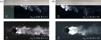
value leads to the formation of permanently visible but unsteady macroscopic cavitation about the jet downstream periphery, as shown in figure 12 for both the unseeded and seeded cases. The unseeded case shows large-volume cavities that coherently shed vortices condensing to clouds of microbubbles with their downstream advection. The microbubbles forming in the jet wake persist far downstream, showing them to be composed of incondensable gas. The concentration gradient between the vapour cavities and liquid volume promotes diffusion of the small quantities of dissolved gas that remain as free gas with cavity condensation and collapse. The distribution of the microbubbles enable visualisation of the shed hairpin-type vortices. For the seeded case the greater density of microbubbles downstream of the jet also permits visualisation of the wake vortices. The influence of
 ${\it\sigma}_{\infty }$
and
 $R$
on established cavitation is described below.
Macroscopic cavity development for
 ${\it\sigma}_{\infty }$
values below 100 % inception (a) with and (b) without artificial nuclei seeding. In both cases permanently visible but unsteady cavities form about the jet downstream periphery, which coherently shed cavitating vortices that condense to clouds of microbubbles with downstream advection.

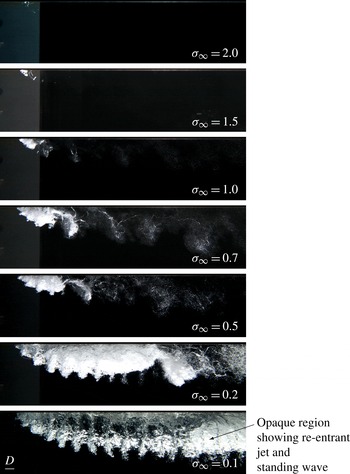
Photographs of cavitation development with reduction of
 ${\it\sigma}_{\infty }$
at
 $R=1.2$
. Two coherent systems become visible and develop with reduction of
 ${\it\sigma}_{\infty }$
: shear-layer vortices on the jet upstream face (negative vorticity) and the hairpin-shaped wake vortices shed from the cavity closure (positive vorticity). The shear-layer vortices condense with their cancellation as they approach the developing shear layer (of opposing vorticity) associated with cavity closure and the hairpin vortex formation. The cavity closure creates a re-entrant jet carrying liquid forward, forming a standing wave within the cavity causing marginal surface breakup and creating the opaque cavity appearance. At the lower
 ${\it\sigma}_{\infty }$
values the cavity leading edge becomes translucent as the standing wave is moved downstream with increasing cavity length (supercavitation).

3.2. General cavitation occurrence and coherent phenomena
As described in the previous section, the freestream nuclei content has a dramatic effect on cavitation inception and cavitation dynamics. With the development of permanently visible macroscopic cavitation for
 ${\it\sigma}_{\infty }$
values below those for
 $P=100\,\%$
, it is assumed that nuclei content no longer has a significant effect, and all tests were carried out without artificial seeding.
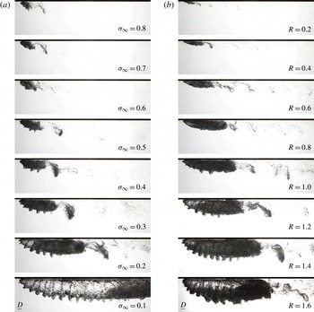
Figure 13 shows a set of images, with
 $R=1.2$
, of reducing
 ${\it\sigma}_{\infty }$
value from close to
 $P=100\,\%$
at
 ${\it\sigma}_{\infty }=2.0$
down to
 ${\it\sigma}_{\infty }=0.1$
, where the cavity length becomes large compared with the jet diameter. At
 ${\it\sigma}_{\infty }=2.0$
the cavitation is similar to the cases discussed above, with transient cavities occurring about the jet downstream periphery. These cavities increase in volume with reduction of
 ${\it\sigma}_{\infty }$
to 1.5 and 1.0. At
 ${\it\sigma}_{\infty }=1.5$
the cavity volume is permanently visible but unsteady. At
 ${\it\sigma}_{\infty }=1.0$
cavitation in the cores of hairpin-shaped vortices shed from the main cavity volume is visible. The cavities condense to microbubble clouds with diffusion and pressure increase as the vortices move downstream. With further reduction of
 ${\it\sigma}_{\infty }$
to 0.7 and 0.5 the main cavity volume continues to increase. The cavitating vortex cores also increase in volume and persist further downstream with corresponding increase in microbubble concentrations. Periodic discontinuities on the cavity upstream surface show the presence of shear-layer instability and vortex formation on the jet upstream face. These vortices are shown to develop on the jet upstream face based on cavity topology, discussed in the next section. Instabilities of the upstream shear layer have been reported on extensively in the literature for single-phase jets in crossflow, as discussed by Megerian et al. (Reference Megerian, Davitian, Alves and Karagozian2007) and in a recent review by Mahesh (Reference Mahesh2013). Their formation is often attributed to Kelvin–Helmholtz instability for higher
 $R$
values, but for lower values other mechanisms have been suggested. Comparison of the present results with previous work for single-phase jets is made below. At
 ${\it\sigma}_{\infty }=0.2$
the formation of the cavitating shear-layer vortices at the cavity leading edge, their growth with advection along the cavity mid-length, and their condensation toward the cavity closure are apparent. Also apparent is the large-volume cavitating hairpin vortex released from the closure region.
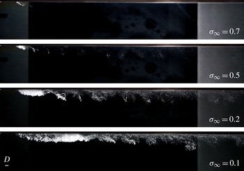
High-speed imaging for
 ${\it\sigma}_{\infty }=0.2$
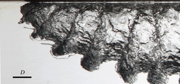
(see supplementary movie 1 available at http://dx.doi.org/10.1017/jfm.2015.73) shows the classical unstable re-entrant jet type closure with periodic vortical ejections stretched in the wake shear layer to form the hairpin-shaped vortices downstream. In the closure region cavity collapse/condensation and stagnation turn the oncoming liquid through 180°, with the re-entrant jet fluid falling under gravity as it approaches the leading edge to form a standing wave within the cavity. The effect of this internal wave is to create turbulence and marginal breakup of the cavity surface. With reduction of
 ${\it\sigma}_{\infty }$
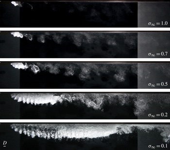
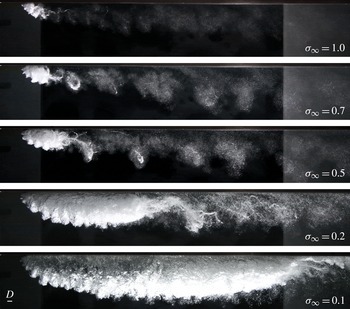
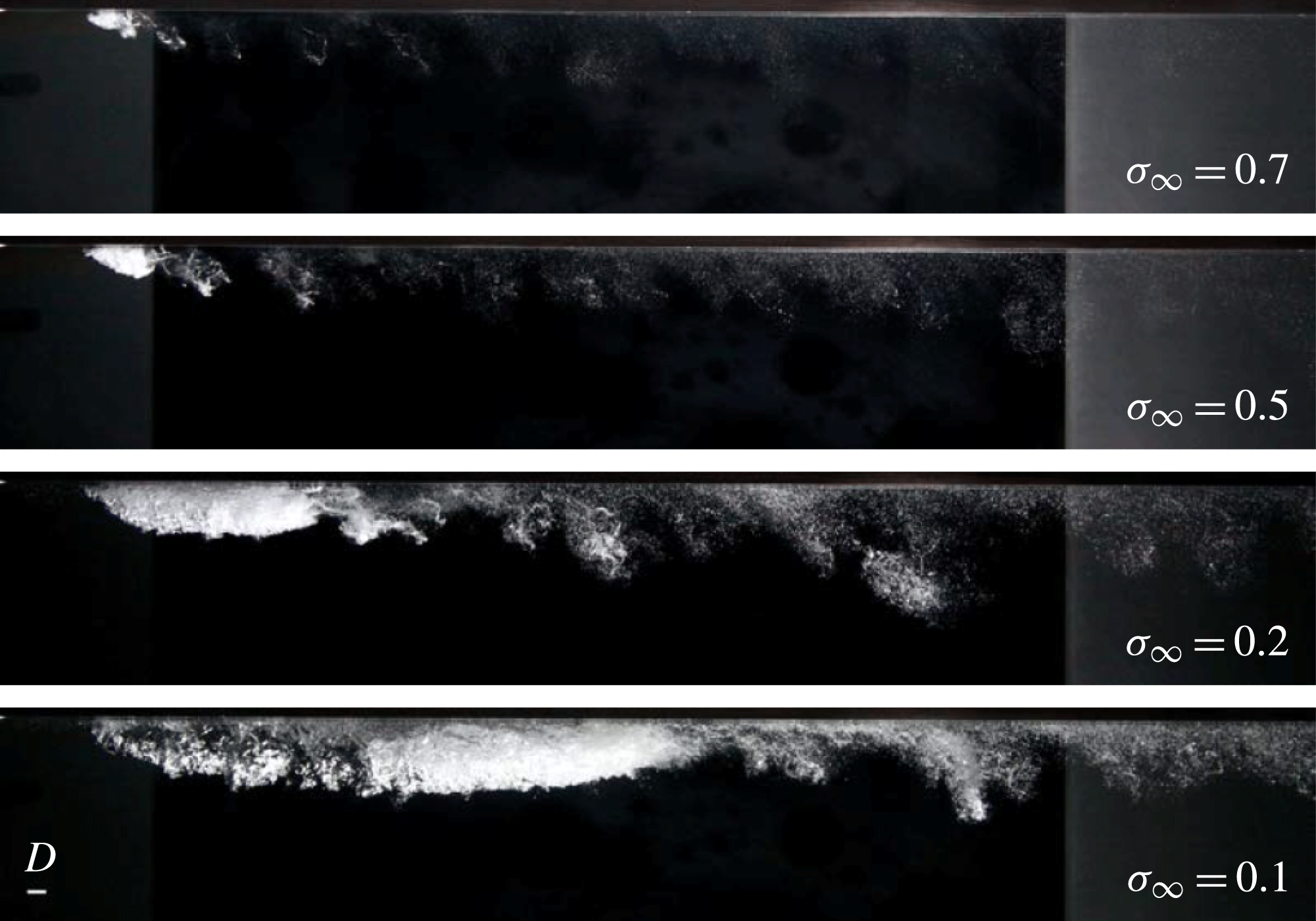
to 0.1 the breaking wave is moved downstream, no longer affecting the cavity surface toward the leading edge (see supplementary movie 2). This is evident where the cavity is glassy and transparent, as opposed to the downstream region where the cavity surface remains mottled and opaque. This effect is more apparent in the far-field image series shown in figure 14 and the back-lit series shown in figure 15. When cavity closure occurs downstream of a solid cavitator this phenomenon is referred to as supercavitation (Franc & Michel Reference Franc and Michel2004). By analogy, once the closure no longer affects the cavity leading edge this is referred to as supercavitation, where in the present context the cavitator is the liquid jet intrusion.
Photographs of cavitation development with reduction of
 ${\it\sigma}_{\infty }$
at
 $R=1.2$
showing coherent shedding of hairpin vortices from the cavity closure. The re-entrant jet associated with cavity closure forms a standing wave within the cavity, causing marginal surface breakup and creating the opaque cavity appearance. At the lower
 ${\it\sigma}_{\infty }$
values the cavity leading edge becomes translucent as the standing wave is moved downstream with increasing cavity length (supercavitation).

Shadow photographs of cavitation development, (a) with reduction of
 ${\it\sigma}_{\infty }$
at
 $R=1.2$
and (b) with increase in
 $R$
at
 ${\it\sigma}_{\infty }=0.2$
, qualitatively showing a power-law relationship between
 ${\it\sigma}_{\infty }$
and
 $l$
, and a linear relationship between
 $R$
and
 $l$
, respectively. For
 $R>0.8$
where the jet penetrates the boundary layer, highly coherent shear layer vortices develop, whereas for
 $R<0.8$
much weaker, less coherent, shear-layer instabilities of opposite sense develop. The standing wave created within the cavity by the closure re-entrant jet is apparent for the long cavities.

The hairpin vortices released from the cavity closure are similar to those observed for single-phase flows generated by the presence of protuberances or jets in crossflows (Acarlar & Smith Reference Acarlar and Smith1987a
,Reference Acarlar and Smith
b
; Ilak et al.
Reference Ilak, Schlatter, Bagheri and Henningson2012). As discussed by Ilak et al. (Reference Ilak, Schlatter, Bagheri and Henningson2012), the mechanism for hairpin generation has been described in detail by Acarlar & Smith (Reference Acarlar and Smith1987a
) and shown to be the result of shear-layer roll-up associated with local regions of slow or reversed flow. In the present case the shear-layer formation varies from close to single-phase at high
 ${\it\sigma}_{\infty }$
values, where the cavity volume is small, through to the cavity closure involving the developed re-entrant jet. The growth in cavity length and volume with reducing
 ${\it\sigma}_{\infty }$
moves the region of hairpin generation progressively further downstream. The volume of the shed hairpins also increases as
 ${\it\sigma}_{\infty }$
is reduced. With the increase in cavity volume and full development of the re-entrant jet, progressively larger volumes of the main cavity are detached in the hairpin formation process. Figure 14 also shows the increase in wavelength of hairpin shedding with reducing
 ${\it\sigma}_{\infty }$
. The high-speed photography shows that the shear-layer vortices rotate in a clockwise direction (negative vorticity) whereas the heads of the hairpins rotate in an anticlockwise direction (positive vorticity). Figure 13 shows, with decreasing
 ${\it\sigma}_{\infty }$
, that the presence and growth of the cavity allow an increasing number of the shear-layer vortices to develop before being rapidly cancelled and reversed in the shear layer of positive vorticity associated with the cavity closure and hairpin formation. In this figure, the image of
 ${\it\sigma}_{\infty }=0.2$
particularly shows the process of the growth of the cavitating shear-layer vortices along the front half of the cavity and their condensation along the downstream half associated with the vorticity reversal.
Increase in
 $R$
above 1.2 results in similar general behaviour. Figure 16 shows a far-field series of reducing
 ${\it\sigma}_{\infty }$
values with
 $R=1.6$
. The most obvious differences are greater main cavity length and height with the increased jet penetration as well as greater volume of the cavitation for both the shear-layer and wake vortices. At
 $R=1.4$
and 1.6, with increasing strength of the shear-layer vortices, the high-speed photography shows pairing of the primary vortices prior to their eventual breakdown toward the trailing edge, as described above. These effects are most evident at the lowest
 ${\it\sigma}_{\infty }$
value of 0.1, as shown in the image series of increasing
 $R$
values in figure 17. Similar general behaviour is also observed for
 $R=1.0$
, but in this case with reduced cavity volumes compared with
 $R=1.2$
.
Photographs of cavitation development with reduction of
 ${\it\sigma}_{\infty }$
at
 $R=1.6$
, showing volume increase in the main cavity and shed vortices compared with lower
 $R$
values.

Photographs of cavitation development with increase in
 $R$
at
 ${\it\sigma}_{\infty }=0.1$
, showing shear layer vortex pairing at the higher
 $R$
values.

With reduction of
 $R$
to 0.8 the shear-layer vortices, as described above for the higher
 $R$
values, are no longer apparent. The cavity surface does, however, show wave-like undulations of similar wavelength to the shear-layer vortices for the higher
 $R$
values but with irregular spacing. Figure 18 shows a far-field image series of reducing
 ${\it\sigma}_{\infty }$
values for
 $R$
= 0.8. This behaviour continues with further reduction of
 $R$
, as shown in the series for
 $R=0.5$
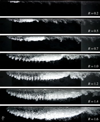
in figure 19. The back-lit images, for constant
 ${\it\sigma}_{\infty }=0.2$
, shown in figure 15 demonstrates the change in shear-layer behaviour with reducing
 $R$
. For
 $R>0.8$
the jet velocity is high enough to penetrate the boundary layer and to generate sufficient negative vorticity for the shear-layer vortices to develop relatively unaffected by boundary layer turbulence. For
 $R<0.8$
, the high-speed photography (see supplementary movie 3) shows that the wave-like undulations on the cavity are not only less coherent but of the opposite sign to the shear-layer vortices for
 $R>0.8$
. This suggests that these undulations are also due to instability of the jet upstream shear layer, but with the effective outer velocity now greater than the jet velocity there is reversal of the velocity gradient, now generating positive vorticity. Hence
 $R=0.8$
is about the critical value (for the present
 ${\it\delta}/D=1.18$
) for reversal of the shear-layer velocity gradient. The lower jet penetration for
 $R<0.8$
also means that the shear-layer instabilities are modulated by boundary layer turbulence of the same positive mean vorticity. This behaviour is similar to film cooling flows, where inclined jets are injected at low
 $R$
values into a turbulent boundary layer. Jovanovic (Reference Jovanovic2006) investigated a round jet injected into a turbulent boundary layer (
 ${\it\delta}/D=0.68$
) at 37° to the horizontal, using laser-induced fluorescence and particle imaging velocimetry. Similar to the present case, strongly coherent vortices of the same sense were found to form in the jet upstream shear layer for
 $R$
values of 1 and 1.5. For
 $R$
values of 0.25 and 0.75, less coherent, more random vortices of the opposite sign to those for the higher
 $R$
values were also similarly found.
Photographs of cavitation development with reduction of
 ${\it\sigma}_{\infty }$
at
 $R=0.8$
, where the highly coherent shear-layer vortices that developed at the higher
 $R$
values no longer develop (compare with figures 13 and 14 for
 $R=1.2$
). The velocity gradient of the jet upstream shear layer reverses direction, from negative to positive vorticity, with reduction of
 $R$
below about 0.8 for the present
 ${\it\delta}/D=1.18$
.

Photographs of cavitation development with reduction of
 ${\it\sigma}_{\infty }$
at
 $R=0.5$
, where the highly coherent shear-layer vortices that developed at the higher
 $R$
values no longer develop (compare with figures 13 and 14 for
 $R=1.2$
). For
 $R<0.8$
the jet no longer penetrates the boundary layer, and much weaker, less coherent, shear-layer instabilities of opposite sense develop compared with the shear-layer vortices that develop for
 $R>0.8$
.

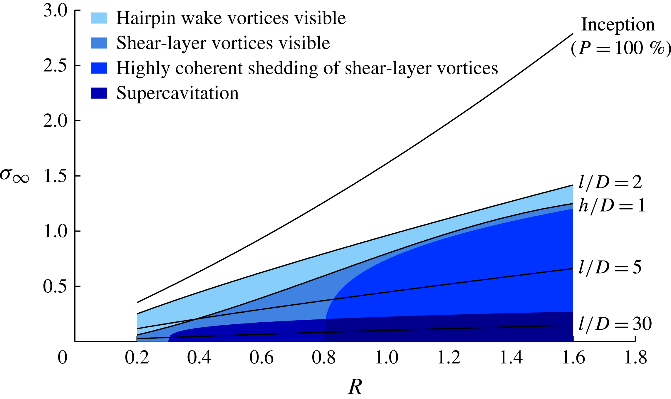
A summary of cavitation development as a function of
 ${\it\sigma}_{\infty }$
and
 $R$
is shown in figure 20. Information on cavity length
 $l$
and height
 $h$
are also shown, which are discussed in detail below. In summary, beyond inception (
 $P=100\,\%$
) an unsteady cavity forms about the wake of the exiting jet that grows in volume with decrease in
 ${\it\sigma}_{\infty }$
or increase in
 $R$
. When the cavity length grows to about
 $2D$
, hairpin-shaped vortices shed in the wake of the main cavity become visible due to cavitation in their cores or remnant microbubble clouds after their condensation. When the cavity height reaches about
 $1D$
, vortices forming in the jet upstream shear layer become visible, and they further develop with reduction of
 ${\it\sigma}_{\infty }$
or increase in
 $R$
. These vortices are highly coherent at
 $R$
values above about 0.8, as shown by the shaded region in figure 20. At
 $R$
values lower than about 0.8 these vortices no longer develop. As the velocity gradient of the jet upstream shear layer reverses, instabilities of the opposite sense are created, randomly modulated by boundary layer turbulence with the reduced penetration. For low enough
 ${\it\sigma}_{\infty }$
values and nearly all
 $R$
values investigated, the supercavitation regime forms where the cavity closure no longer affects the cavity leading edge.
Summary of cavitation phenomena about a jet in crossflow as a function of
 $R$
and
 ${\it\sigma}_{\infty }$
. Beyond inception an unsteady cavity forms about the wake of the exiting jet, and grows in volume with decrease in
 ${\it\sigma}_{\infty }$
or increase in
 $R$
. Hairpin-shaped vortices shed in the wake of the main cavity become visible first with decreasing
 ${\it\sigma}_{\infty }$
. With further decrease in
 ${\it\sigma}_{\infty }$
or increase in
 $R$
, vortices forming in the jet upstream shear layer become visible. These are highly coherent for
 $R>0.8$
, as shown by the shaded region. At
 $R<0.8$
these vortices no longer develop. At these lower
 $R$
values the velocity gradient of the jet upstream shear layer reverses, creating instabilities of the opposite sense randomly modulated by boundary layer turbulence with the reduced jet penetration. At low
 ${\it\sigma}_{\infty }$
values the supercavitation regime forms, where the cavity closure no longer affects the leading edge.

3.3. Cavity geometry and topology
Images were acquired at regular intervals over the cavitating region shown in figure 20, from which information on cavity length and height as a function of
 ${\it\sigma}_{\infty }$
and
 $R$
were derived. Cavity length is defined from leading to trailing edge and the cavity height from the ceiling to the middle of the shear layer. These data show that the cavity length has a linear dependence on
 $R$
and a power-law dependence on
 ${\it\sigma}_{\infty }$
. These relations may be seen qualitatively from the image series shown in figure 15 for constant
 $R$
and
 ${\it\sigma}_{\infty }$
values. Linear and nonlinear inviscid theories for small cavitation numbers give cavity length as a power law, and experimental results may often be closely modelled with such a relation (Franc & Michel Reference Franc and Michel2004; Pearce & Brandner Reference Pearce and Brandner2014). For the present results
 $l/D=1.9R{\it\sigma}_{\infty }^{-1.2}$
is found from a least-squares fit. Some contours of constant
 $l/D$
are shown in figure 20. The cavity height is not as easily modelled by a simple relation but for
 ${\it\sigma}_{\infty }<0.5$
may be approximated by
 $h/D=0.3(3+R)R{\it\sigma}_{\infty }^{-0.5}$
. Empirical equations for single-phase jet trajectory are monotonic (Mahesh Reference Mahesh2013) and therefore not suitable for the present cavitating jet in crossflow.
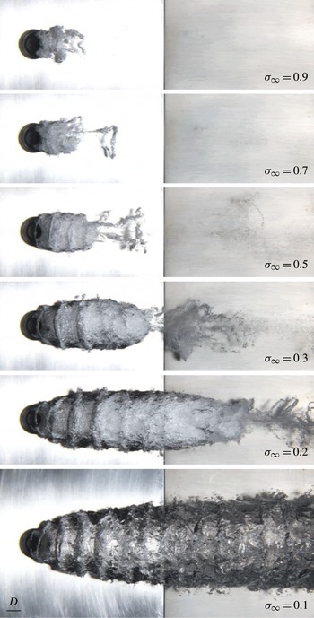
Figure 21 shows a series of images with reducing
 ${\it\sigma}_{\infty }$
value for
 $R=1.2$
, taken from below the jet. For all
 ${\it\sigma}_{\infty }$
values shown, the cavity leading edge detaches from the downstream circumference of the jet nozzle around about a 180° arc, increasing slightly with reduction in
 ${\it\sigma}_{\infty }$
. The hairpin-shaped wake vortices are visible for all
 ${\it\sigma}_{\infty }$
values and are more evident for
 ${\it\sigma}_{\infty }=0.7$
, 0.5 and 0.3 in figure 21. For
 ${\it\sigma}_{\infty }\leqslant$
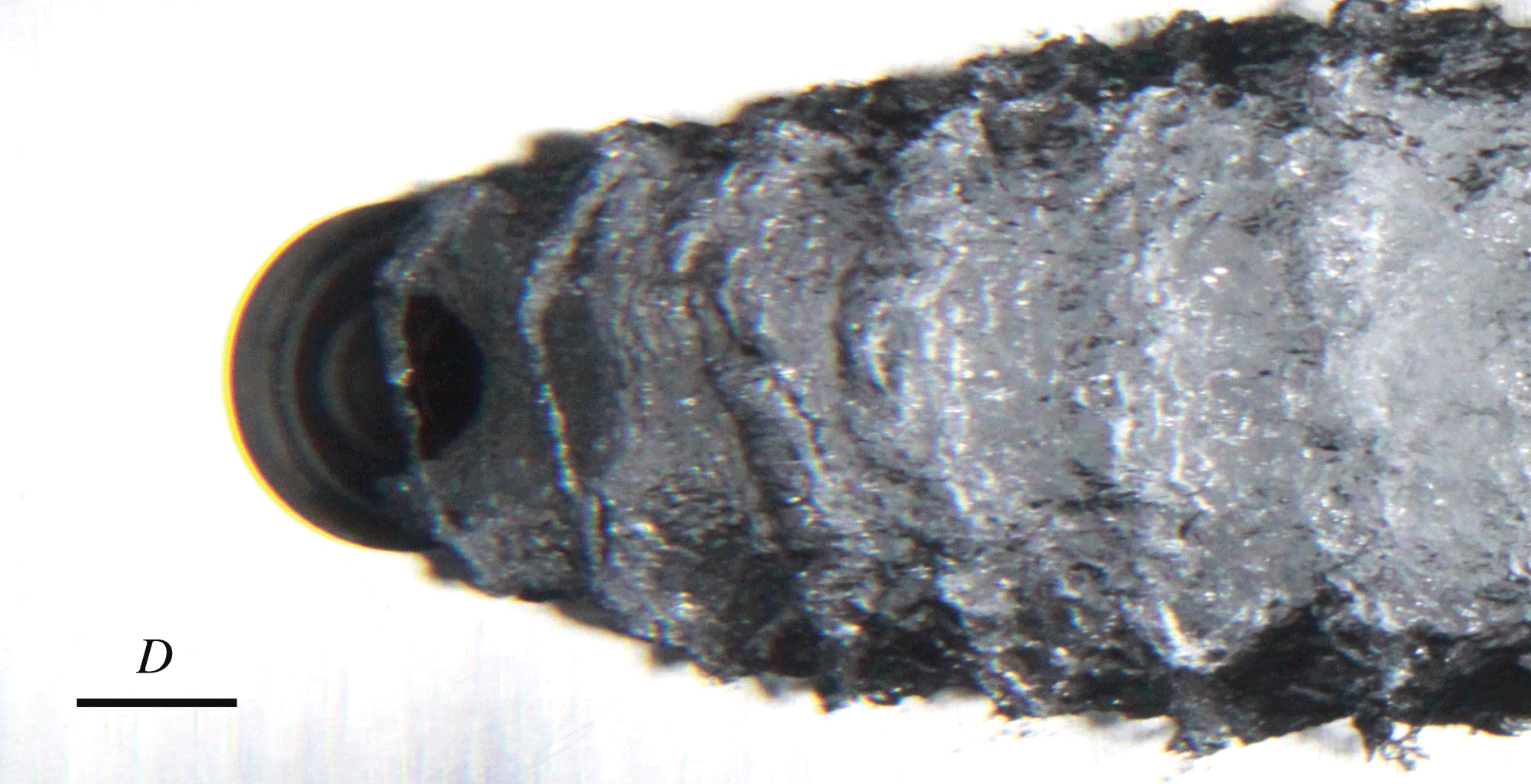
0.5 the cavitating shear-layer vortices become apparent. In each case the first two or three cavitating vortex cores can be seen to partially or fully bridge the upstream periphery of the exiting jet from either side of the main cavity volume (showing that these originate from upstream shear-layer instability). Figure 22 shows a magnified image from below for
 ${\it\sigma}_{\infty }=0.2$
and
 $R=1.2$
showing this topology in more detail, and figure 23 shows a magnified image from the side for
 ${\it\sigma}_{\infty }=0.1$
and
 $R=1.2$
.
Photographs from beneath the jet of cavitation development with reduction of
 ${\it\sigma}_{\infty }$
at
 $R=1.2$
. The cavity leading edge detaches from the downstream circumference of the jet nozzle around about a 180° arc, increasing slightly with reduction in
 ${\it\sigma}_{\infty }$
. The hairpin-shaped wake vortices are visible for all
 ${\it\sigma}_{\infty }$
values. For
 ${\it\sigma}_{\infty }\leqslant$
0.5 the cavitating shear-layer vortices become apparent. In each case the first two or three cavitating vortex cores can be seen to partially or fully bridge the upstream periphery of the exiting jet from either side of the main cavity volume, showing that these originate from upstream shear-layer instability.

Magnified image from beneath the jet for
 ${\it\sigma}_{\infty }=0.2$
and
 $R=1.2$
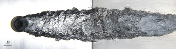
showing cavity topology associated with initial formation of vortices within the jet upstream shear layer.

Magnified image from the side for
 ${\it\sigma}_{\infty }=0.1$
and
 $R=1.2$
showing cavitating cores of secondary streamwise vortices between the primary spanwise rolls.

The still and high-speed images show that the shear-layer vortices originate within
 $1D$
of the exit and at a shallow angle to the wall, rotating to normal to the wall with jet deflection, as can be seen in figure 23. The cavitating cores develop as tendrils or ligaments, drawn from either side of the main cavity, that grow over the deflected jet with downstream advection. The jet fluid is deformed from the exiting round cross-section to a thin broad section several diameters wide within the first two or three vortex wavelengths, further widening with downstream cavity growth. The bridging cavitating cores in most cases connect as the vortices move downstream, simultaneously stretched around the widening jet and inflating main cavity. The vortices then undergo a process of breakup and condensation with advection along the cavity length, with their ultimate dissipation at the cavity closure. This is due to the vorticity reversal associated with the developing shear layer approaching the cavity closure, as described in the previous section. The cores condense within three or four wavelengths (depending on cavity length) followed by turbulent breakup and dissipation, leaving remnant microbubble clouds as they approach the cavity closure. After the initial condensation, further downstream propagation on the main cavity is manifested as regular wave-like circumferential discontinuities decreasing in amplitude with the progressive turbulent breakup and dissipation along the cavity length. Unlike single-phase jets in crossflow, no significant vortical structures or turbulent mixing occur below the jet due to the presence of the cavity. Where the cavity is present this limits the turbulent mixing and jet breakup to essentially the upstream shear-layer vortices only. The cavity is a free surface, however, on which instabilities can also develop between the liquid and vapour phases. For the higher
 $R$
values, where the vortex cores in the jet upstream shear layer are cavitating, undulations on the main cavity surface below are apparent at low
 ${\it\sigma}_{\infty }$
values. However, these initial undulations may only be associated with the formation of the jet upstream shear-layer instabilities, as suggested by side images. As a free surface the cavity provides surface tension as another mechanism for damping and dissipation of turbulent fluctuations.
The shear-layer vortices extend almost around the entire circumference of the main cavity, as shown in figure 23. Figure 23 also shows that the main cavity is separated from the wall by a thin liquid layer. This would suggest a stagnation on the vertical centreplane between the cavity and the wall due to the meeting of circumferential flow driven by the spanwise shearing of jet fluid by the main flow. The back-lighting reveals the presence of cavitating cores of secondary streamwise vortices between the primary spanwise rolls. The wavelength of the shear-layer vortices for this example (
 $R=1.2$
,
 ${\it\sigma}_{\infty }=0.1$
) is about
 $1.5D$
, varying slightly along the cavity. The variation of wavelength of the shear-layer vortices with
 $R$
and
 ${\it\sigma}_{\infty }$
is discussed below. The less coherent wake vortices have wavelengths typically of several jet diameters. The wavelength tends to increase with decreasing
 ${\it\sigma}_{\infty }$
or increasing
 $R$
, i.e. with increasing cavity volume. The relationship between the shear-layer and wake vortices is discussed below.
For
 $R<0.8$
, where the jet upstream shear-layer velocity gradient reverses, the cavity no longer exhibits the regular corrugated structure as with the higher
 $R$
values. Figure 24 shows an image from below for
 $R=0.6$
and
 ${\it\sigma}_{\infty }=0.1$
, typically demonstrating the irregular cavity surface for
 $R<0.8$
– similarly to the images from the side discussed in the previous section. As described in the previous section, the jet becomes increasingly more affected by boundary layer turbulence with reduction of
 $R$
due to decreasing velocity and penetration. This effect is further enhanced with the jet upstream shear-layer vorticity, now of the same sense as the mean boundary layer vorticity. Figure 24 typically shows for the low
 $R$
values that no cavitation occurs in the cores of the now less coherent, lower-strength, shear-layer vortices.
Still photograph from beneath the jet for
 $R=0.6$
and
 ${\it\sigma}_{\infty }=0.1$
, typically demonstrating the irregular cavity surface for
 $R<0.8$
. For
 $R<0.8$
the jet no longer penetrates the boundary layer, and much weaker, less coherent, shear-layer instabilities of opposite sense develop compared with the shear-layer vortices that develop for
 $R>0.8$
.

3.4. Shear-layer and wake vortex characteristic frequencies
As discussed in § 2, cavity dynamics were analysed using image sequences from high-speed photography. Time series were derived by spatially averaging pixel intensity from regions of interest. Figure 2 shows the typical locations sampled to determine the shedding frequencies of the shear-layer and wake vortices. As described in § 3.2, for
 $R\geqslant 0.8$
the shear-layer vortices are highly coherent, for which wavelet analysis was used to determine the shedding frequencies. The Morlet-6 wavelet correlates over multiple events and was chosen as most suitable for frequency analysis of these near-periodic events. The shedding frequencies as a function of
 ${\it\sigma}_{\infty }$
and
 $R$
were then found from the wavelet power spectral density in each case. The frequencies of the less coherent cases of the shear-layer vortices (
 $R<0.8$
) and the similarly less coherent wake vortices were found directly by direct event counting from the derived time series. Uncertainties for both analysis techniques were estimated from the number of ambiguous events and thresholding sensitivity. For the shear-layer vortices, for
 $R>0.8$
, estimated uncertainties vary from about
 $\pm 3\,\%$
to
 $\pm 1\,\%$
for
 $R$
values from 0.8 to 1.6 respectively. For
 $R<0.8$
the estimated uncertainty is about 10 %. For the hairpin vortices the estimated uncertainties vary from about
 $\pm 10\,\%$
to
 $\pm 12\,\%$
between the lowest to highest
 $R$
values respectively.
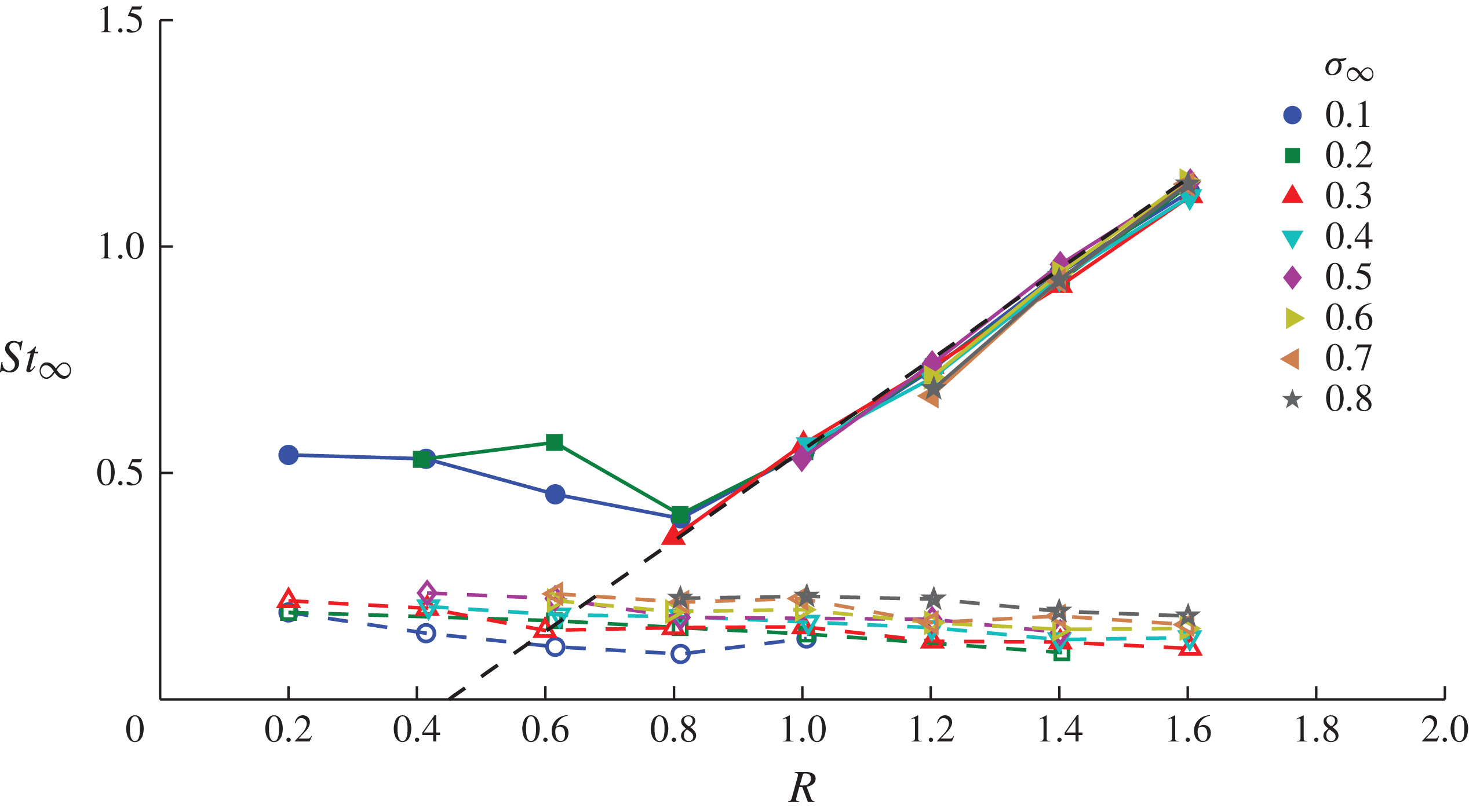
Figure 25 shows the derived shear-layer and hairpin vortex shedding frequencies non-dimensionalised using a freestream-velocity-based Strouhal number,
 $\mathit{St}_{\infty }=fD/U_{\infty }$
. The ranges of
 $R$
and
 ${\it\sigma}_{\infty }$
for which frequencies were measured are limited to whether the vortices developed and cavitation made them visible or whether they could be imaged (see supplementary movie 4). The shear-layer vortices are shed at frequencies varying close to linearly with
 $R$
for
 $R\geqslant 0.8$
(
 $\mathit{St}_{\infty }=R-0.45$
) and are independent of
 ${\it\sigma}_{\infty }$
. The advection speed of the shear-layer vortices has been determined from correlation of extracted time series from two streamwise points within the shear layer. The speed was determined at multiple locations along the cavities for
 $R\geqslant 1$
and
 $0.2\leqslant {\it\sigma}_{\infty }\leqslant 0.6$
. At the initial formation, the speed of the vortices is less than
 $U_{\infty }$
, and they accelerate along the cavity length to values between
 $U_{J}$
and
 $U_{\infty }$
. The wavelength correspondingly increases along the cavity length. The speed and wavelength are mildly dependent on
 ${\it\sigma}_{\infty }$
, due to changes in cavity length as the longer cavities permit the advection speed to develop before the vortices condense. The developed wavelength varies with
 $R$
from about
 $1.8D$
at
 $R=1$
to values ranging between
 $0.8D$
and
 $1.4D$
at
 $R=1.6$
(depending on
 ${\it\sigma}_{\infty }$
, or equivalently cavity length). For
 $R<0.8$
, where the shear-layer vortices have reversed direction, the frequencies tend to increase slightly with decreasing
 $R$
, suggesting possibly the varying effect of boundary layer turbulence with decreasing jet penetration.
Shear-layer (closed symbols) and hairpin (open symbols) vortex shedding frequencies derived from high-speed imaging. Shear-layer vortices are shed at frequencies varying close to linearly with
 $R$
for
 $R\geqslant 0.8~(\mathit{St}_{\infty }=R-0.45)$
and are independent of
 ${\it\sigma}_{\infty }$
. For
 $R<0.8$
, where the shear-layer vortices have reversed direction, the frequencies tend to increase slightly with decreasing
 $R$
, possibly due to boundary layer turbulence. Shedding frequencies for the wake vortices show a general independence of
 $R$
for all
 ${\it\sigma}_{\infty }$
values, showing the two vortex systems to be essentially independent of each other.

The shedding frequencies for the wake vortices show a general independence of
 $R$
for all
 ${\it\sigma}_{\infty }$
values within the estimated uncertainties. For all
 $R$
values except the lowest, there is a consistent decrease in frequency with decreasing
 ${\it\sigma}_{\infty }$
due to increasing cavity volume. For
 $R\geqslant 0.8$
the shear-layer shedding frequencies vary from about six times the hairpin frequencies at the highest
 $R$
to about twice for
 $R$
= 0.8. Apart from the increasing negative vorticity generated by the shear-layer vortices with increasing
 $R$
possibly affecting the hairpin generation, these data would show the two vortex systems to be essentially independent of each other for all
 $R$
and
 ${\it\sigma}_{\infty }$
values.
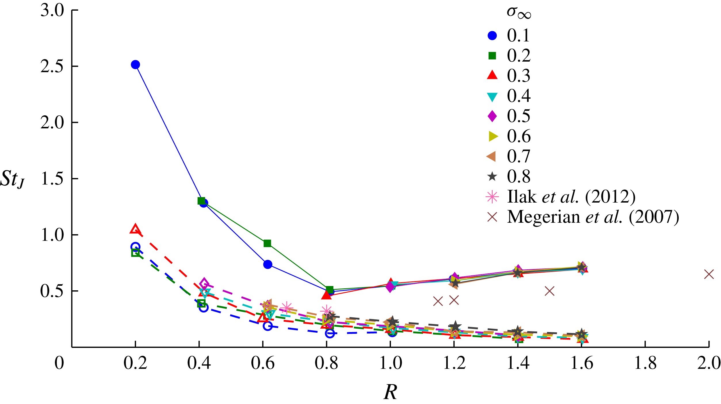
Shedding frequencies of coherent structures associated with jets in crossflow are commonly non-dimensionalised using a jet-velocity-based Strouhal number
 $\mathit{St}_{J}=fD/U_{J}$
. The data shown in figure 25 are replotted in figure 26 for the purpose of comparing the present data with previous results from single-phase studies. Due to the relatively high
 $\mathit{Re}_{J}$
values and low
 $R$
values for the present work compared with previous, there is limited data for single-phase jets in crossflow with which to make comparisons. Nevertheless, some comparisons can be made using the results from Megerian et al. (Reference Megerian, Davitian, Alves and Karagozian2007) and Ilak et al. (Reference Ilak, Schlatter, Bagheri and Henningson2012). Megerian et al. (Reference Megerian, Davitian, Alves and Karagozian2007) presented results from wind tunnel tests of a nitrogen jet in crossflow for various configurations of a flush or raised nozzle, with and without frequency forcing. Hotwire frequency measurements of the jet upstream shear-layer instabilities were made between 0.1 and 3 jet diameters downstream of the jet exit. For the flush nozzle case without forcing, measurements were made at
 $\mathit{Re}_{J}=2000$
with
 ${\it\delta}/D<2$
over a range of
 $R$
values that overlap with the present results (for which
 $\mathit{Re}_{J}$
varied from
 $25\times 10^{3}$
to
 $160\times 10^{3}$
and
 ${\it\delta}/D=1.18$
). These data are plotted in figure 26 and show a similar linear trend, but offset to the present shear-layer data. This offset could be attributed to the large difference in
 $\mathit{Re}_{J}$
. The hairpin vortex shedding frequencies can be compared with the results by Ilak et al. (Reference Ilak, Schlatter, Bagheri and Henningson2012) from direct numerical simulation. These results were obtained for
 $R$
values of 0.675 and 0.8 at corresponding
 $\mathit{Re}_{j}$
values of 334 and 396 with a laminar wall boundary layer for which
 ${\it\delta}/D$
is about 0.9. Their stability analysis showed that the hairpin vortices develop at
 $R=0.675$
, for which
 $\mathit{St}_{j}=0.35$
and for
 $R=0.8$
,
 $\mathit{St}_{J}=0.32$
. These points are plotted in figure 26. Although these results are for a different flow regime they show close comparison with the high
 ${\it\sigma}_{\infty }$
values from the present results, where cavitation is limited such that the flow is close to single-phase. The present data in turbulent flow suggest the hairpin frequencies are close to independent of
 $R$
. The
 $\mathit{St}_{\infty }$
values corresponding to the above
 $\mathit{St}_{J}$
values from Ilak et al. (Reference Ilak, Schlatter, Bagheri and Henningson2012) are 0.24 and 0.26. These comparisons, although limited, show some correlation and demonstrate the requirement for further comparison of experimental and computational results for greater ranges of
 $\mathit{Re}$
,
 $R$
and
 ${\it\sigma}_{\infty }$
values.
Results shown in figure 25 non-dimensionalised as a jet-velocity-based Strouhal number,
 $\mathit{St}_{J}$
, for comparison with the experimental results of Megerian et al. (Reference Megerian, Davitian, Alves and Karagozian2007) for shear-layer frequencies and the computational results of Ilak et al. (Reference Ilak, Schlatter, Bagheri and Henningson2012) for hairpin frequencies. The results from Megerian et al. (Reference Megerian, Davitian, Alves and Karagozian2007) (
 $\mathit{Re}_{J}=2000$
) show a similar trend to the present results (
 $\mathit{Re}_{J}$
varied from
 $25\times 10^{3}$
to
 $160\times 10^{3}$
) but offset possibly due to the large difference in Reynolds number. The results by Ilak et al. (Reference Ilak, Schlatter, Bagheri and Henningson2012), (laminar flow) show close comparison with the high
 ${\it\sigma}_{\infty }$
values from the present results where the flow is close to single-phase despite the different flow regimes.

The time series obtained for each vortex system have been further examined to investigate the degree of periodicity as a function of
 $R$
and
 ${\it\sigma}_{\infty }$
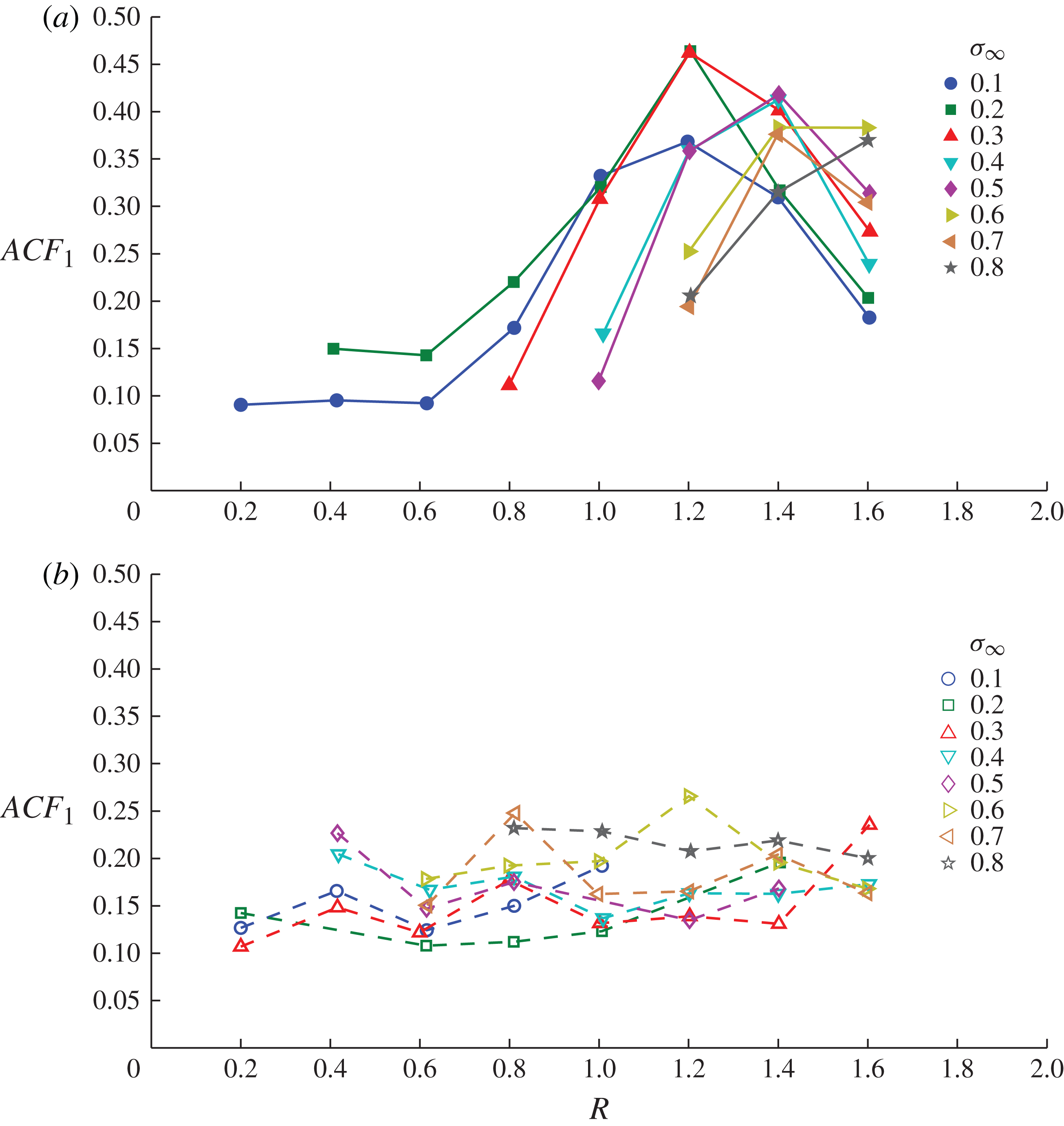
. Figure 27 shows the magnitude of the first peak of the autocorrelation (
 $\mathit{ACF}_{1}$
) for each time series as a function of
 $R$
and
 ${\it\sigma}_{\infty }$
for the shear-layer and hairpin vortices. In both cases the magnitudes follow trends with
 $R$
and
 ${\it\sigma}_{\infty }$
consistent with the qualitative and quantitative data discussed above. The hairpin vortices are not highly coherent, and show a consistently low magnitude for all
 $R$
and
 ${\it\sigma}_{\infty }$
values. The shear-layer vortices show a similar magnitude to the hairpin vortices at low
 $R$
values where the shear-layer development is driven by the turbulent boundary layer flow. The magnitudes increase with increase in
 $R$
, reflecting the highly periodic or coherent nature of the shear-layer vortices at the higher
 $R$
values, where the shear-layer development is driven by the now higher jet velocity with sufficient penetration to be free of the effect of boundary layer turbulence. The reduction in
 $\mathit{ACF}_{1}$
at the highest
 $R$
value may be the result of vortex pairing and/or merging of vortices due to increase in cavity volume (see supplementary movie 5). At the higher
 $R$
values the decrease in
 $\mathit{ACF}_{1}$
with increase in
 ${\it\sigma}_{\infty }$
reflects reduced coherence, when the cavity length becomes similar to the wavelength of the shear-layer vortices (see supplementary movie 6).
Magnitude of the first peak of the autocorrelation (
 $\mathit{ACF}_{1}$
) of the time series derived from high-speed imaging as a function of
 $R$
and
 ${\it\sigma}_{\infty }$
for (a) shear-layer and (b) hairpin vortices. The hairpin vortices are not highly coherent and show a consistently low magnitude for all
 $R$
and
 ${\it\sigma}_{\infty }$
values. The shear-layer vortices show a similar magnitude to the hairpin vortices at low
 $R$
values, where the shear-layer development is driven by the turbulent boundary layer flow. The magnitudes increase with increase in
 $R$
, reflecting the highly periodic or coherent nature of the shear-layer vortices at the higher
 $R$
values, where the shear-layer development is driven by the now higher jet velocity with sufficient penetration to be free of the effect of boundary layer turbulence.

4. Conclusions
Cavitation occurrence about a jet in crossflow at a relatively high Reynolds number exhibits a broad range of phenomena depending on the cavitation number and jet to freestream velocity ratio. Cavitation inception involves a dynamic process ranging over cavitation numbers of order 0.1–10 depending on flow conditions. Inception involves the intermittent formation of localised cavities in the high-shear regions either side of the exiting jet, the nature and probability of which depends on the nuclei content within the approaching boundary layer, the cavitation number and the velocity ratio. The inception process can be characterised acoustically using an intermittency approach to quantify the duration or probability of cavitation occurrence with reduction of the cavitation number for bounding cases of low and high susceptibility to phase change. For low susceptibility to phase change, where there are sparse high-strength nuclei, inception occurs at low cavitation numbers, involving intermittent cavity formation that increases in occurrence or duration, from 0 to 100 % over a small range of cavitation numbers. For the high-susceptibility case, where there are abundant low-strength nuclei, the process involves frequent short duration events due to the large number of individual nuclei excitations varying from 0 to 100 % occurrence over a large range of cavitation numbers.
With reduction of the cavitation number beyond inception, an unsteady macroscopic cavity forms in the wake of the jet, from which hairpin vortices are coherently shed. These vortices are made visible either by cavitation within their cores or by remnant incondensable gas after their condensation. The cavity length grows with a power-law dependence on the cavitation number and with a linear dependence on the jet to freestream velocity ratio. The cavity closure remains unstable with reduction of the cavitation number and continues to coherently shed hairpin vortices. The hairpin vortices are generated by the same mechanisms as those forming in the wake of jets in crossflows or protuberances in single-phase flow. The hairpin shedding frequency is independent of the velocity ratio but decreases with reducing cavitation number and cavity volume growth. As the cavity length grows, the closure develops a liquid re-entrant jet, forming a breaking wave within the cavity that is progressively moved downstream with increase in cavity length. For sufficiently low cavitation numbers the projection of the re-entrant jet fluid no longer reaches the cavity leading edge, analogous to supercavitation forming about solid cavitators.
In addition to the hairpin vortices forming about the cavity closure, cavitating vortices form along the leading part of the cavity due to instability of the jet upstream shear layer. For jet to freestream velocity ratios greater than about 0.8, where negative vorticity is generated and the jet penetrates the wall boundary layer, these vortices are highly coherent. The shear-layer vortices form close to the wall and fully bridge the exiting jet for low cavitation numbers. The vortex shedding frequency increases linearly with increase in the velocity ratio independent of the cavitation number. The speed and wavelength of the vortices develop along the cavity, dependent on cavity length, and are therefore dependent on
 $R$
and
 ${\it\sigma}_{\infty }$
. The shear layer of positive vorticity developing over the trailing part of the cavity associated with the cavity closure and the hairpin vortex formation causes rapid reversal and condensation of the shear-layer vortices as they approach the cavity closure.
For jet to freestream velocity ratios less than 0.8, the highly coherent shear-layer vortices no longer develop. At these lower velocity ratios the velocity gradient of the jet upstream shear layer reverses, creating instabilities of the opposite sense randomly modulated by boundary layer turbulence with the reduced jet penetration.
For velocity ratios greater than 0.8, the shear-layer shedding frequencies vary from about twice to six times the hairpin frequencies for velocity ratios between 0.8 and 1.6 respectively. Within the precision of the measured shedding frequencies these two vortical systems appear independent of each other. Frequency analysis of the coherent structures could be carried out using high-speed imaging of the cavitation, provided that the structures developed were made visible by cavitation and could be imaged.
Hairpin vortex shedding frequencies computed by direct numerical simulation (Ilak et al. Reference Ilak, Schlatter, Bagheri and Henningson2012) for a single-phase jet in crossflow with a similar jet diameter to boundary layer thickness ratio compare closely with the present results at the high cavitation numbers despite the different flow regimes. Shear-layer vortex shedding frequencies were measured by Megerian et al. (Reference Megerian, Davitian, Alves and Karagozian2007) for a single-phase jet in crossflow with a similar jet diameter to boundary layer thickness ratio. These data show a common trend with jet to freestream velocity ratio with the present data but with a lower frequency offset, possibly due to the large Reynolds number difference.
Suggestions for future work would include more detailed investigation of the inception process and the mechanisms for noise generation and the role of the boundary layer and effect of the Reynolds and cavitation numbers on development of coherent phenomena in single-phase and cavitating cases.
Supplementary movies
Supplementary movies are available at http://dx.doi.org/10.1017/jfm.2015.73.
Acknowledgements
The authors wish to acknowledge the assistance of Mr M. Nijland and Mr K. Croci in the experimental setup and acquisition of the data for the presented work, and the support of the University of Tasmania and the Australian Defence Science and Technology Organisation.