Introduction
In the past three decades, efforts have been made to couple instrumented indentation with resistive measurements.[Reference Nili, Kalantar-Zadeh, Bhaskaran and Sriram1] This development was driven by several motivations, such as the local monitoring of phase transformation,[Reference Clarke, Kroll, Kirchner, Cook and Hockey2–Reference Ruffell, Bradby, Fujisawa and Williams8] the study of native oxide fracture,[Reference Pethica and Tabor9–Reference Nguyen, Wei and Lin11] the investigation of MEMS operation at small scales,[Reference Duvivier, Mandrillon, Inal, Dieppedale, Deldon-Martoscia and Polizzi12,Reference Arrazat, Duvivier, Mandrillon and Inal13] and the contact area computation during nanoindentation test.[Reference Fang, Muhlstein, Collins, Romasco and Friedman14,Reference Sprouster, Ruffel, Bradby, Stauffer, Major, Warren and Williams15] The later point is of particular interest for the determination of the contact area A c which is essential to compute both the sample Young's modulus and the hardness from nanoindentation tests:
➢ The sample Young's modulus is determined using the Sneddon's relation[Reference Sneddon16]:
(1)with S c the contact stiffness (measured continuously during nanoindentation test) and E* the reduced modulus, expressed as: $$S_{\rm c} = \displaystyle{2 \over {\sqrt \pi}} E{^\ast}\sqrt {A_{\rm c}} $$(2)with v tip, v sample, E tip, E sample the tip and sample Poisson's ratios and moduli, respectively.$$E{^\ast} = \left( {\displaystyle{{1-v_{{\rm tip}}^2} \over {E_{{\rm tip}}}} + \displaystyle{{1-v_{{\rm sample}}^2} \over {E_{{\rm sample}}}}} \right)^{-1}$$
➢ The sample hardness H is computed using Eq. (3), with L the load on the sample.


 $$H = \displaystyle{L \over {A_{\rm c}}}$$
The contact area A c (defined as the projected area of the contact interface between the tip and the sample) is however complex to monitor, even for the simplest case of homogeneous semi-infinite specimens. This is because the contact area depends both on the tip geometry and on the contact depth h c [h c being the length of the tip effectively in contact with the sample (Supplementary Fig. S1)]. The tip geometry is either determined by AFM imaging or by using a calibration sample with well-known mechanical properties.[Reference Oliver and Pharr17] As shown in Supplementary Fig. S1, the contact depth h c depends on sample rheology: the sample can either sink-in or pile-up around the tip during nanoindentation. The contact depth h c then strongly differs from the total penetration depth H (which is the depth reached by the tip from the initial specimen surface).
The standard methods widely used to extract contact area require analytical models based on material rheology assumptions, which use penetration depth and contact stiffness values to compute the contact depth.[Reference Oliver and Pharr18,Reference Loubet, Bauer, Tonck, Bec, Gauthier-Manuel, Nastasi, Parkin and Gleiter19] On the contrary, the direct monitoring of the contact area by resistive-nanoindentation brings supplementary inputs to the quantitative analysis of indentation tests. This is expected to be an experimental alternative to standard analytical models.
A first attempt to extract mechanical contact area from electrical measurements was reported by Fang et al.[Reference Fang, Muhlstein, Collins, Romasco and Friedman14] for micro-indentation. The authors successfully related non-linear current-bias curves performed during micro-indentation to real-time contact area. However, this approach is inadequate for nanoindentation. More promising results were obtained by Sprouster et al.,[Reference Sprouster, Ruffel, Bradby, Stauffer, Major, Warren and Williams15] with resistive nanoindentation performed on a gold bulk sample with a vanadium carbide tip. The measured resistance during indentation was successfully fitted using an analytical model based on Maxwell expression for the spreading resistance [Eq. (4), with ρ the material resistivity and r c the contact radius]. With this method, the authors managed to compute their specimen resistivity but the ability to monitor the contact area during nanoindentation was not discussed.
 $$R_{{\rm spreading}} = \displaystyle{\rho \over {4r_{\rm c}}}$$
In the present work, a complete method is proposed to compute the contact area using resistive-nanoindentation of noble metals. First, the different contributions to the measured resistance are discussed, then the computation procedure is detailed and applied step-by-step: (1) measurement of the tip shape, (2) set-up calibration on a model specimen (gold bulk single crystal), and (3) extraction of the contact area on a specimen with complex rheology (gold film on sapphire substrate), and finally, the data generated by this method are compared to experimental AFM measures of contact areas.
Experimental details
Nanoindentation testing is performed with a home-made device, which includes a commercial actuator from Nanomechanics Inc (Oak Ridge, TN, USA). Resistance measurements are conducted with a ResiScope apparatus from Scientec.[Reference Houzé, Meyer, Schneegans and Boyer20] Nanoindentation tests are performed with a Berkovich boron-doped diamond (BDD) tip with resistivity in the range [0.2–2] Ω.cm. Resistive-nanoindentation tests were performed on a gold bulk single crystal (100) for the calibration step, and the whole method was validated on a 200 nm-thick polycrystalline gold film deposited on a sapphire substrate. Gold samples were chosen as model specimens, due to the absence of native oxide. Nonetheless, this method can be applied to any oxide-free highly-conductive material. Indentation of a composite geometry such as an elasto-plastic film (gold) on an elastic substrate (sapphire) is a model case of complex rheology which is depth-dependent and where no analytical modeling exists. AFM imaging of residual imprints is performed after each test for validation purpose. Post-mortem contact areas are computed using Gwyddion software[21]: a map of local plane inclination angles is first extracted from the topological map of these imprints.[Reference Charleux, Keryvin, Nivard, Guin, Sangleboeuf and Yokoyama22] Then manually-adjusted edge detection is performed on the obtained map (standard deviation on the contact area lower than 3%). AFM images are performed after the final elastic unloading (viscous relaxation is negligible at room temperature): this leads to a small modification of the indentation imprint, as compared to the contact area under loading. According to Charleux et al.,[Reference Charleux, Keryvin, Nivard, Guin, Sangleboeuf and Yokoyama22] the induced error on the contact area is lower than 10%.
Results and discussion
Resistive-nanoindentation curves
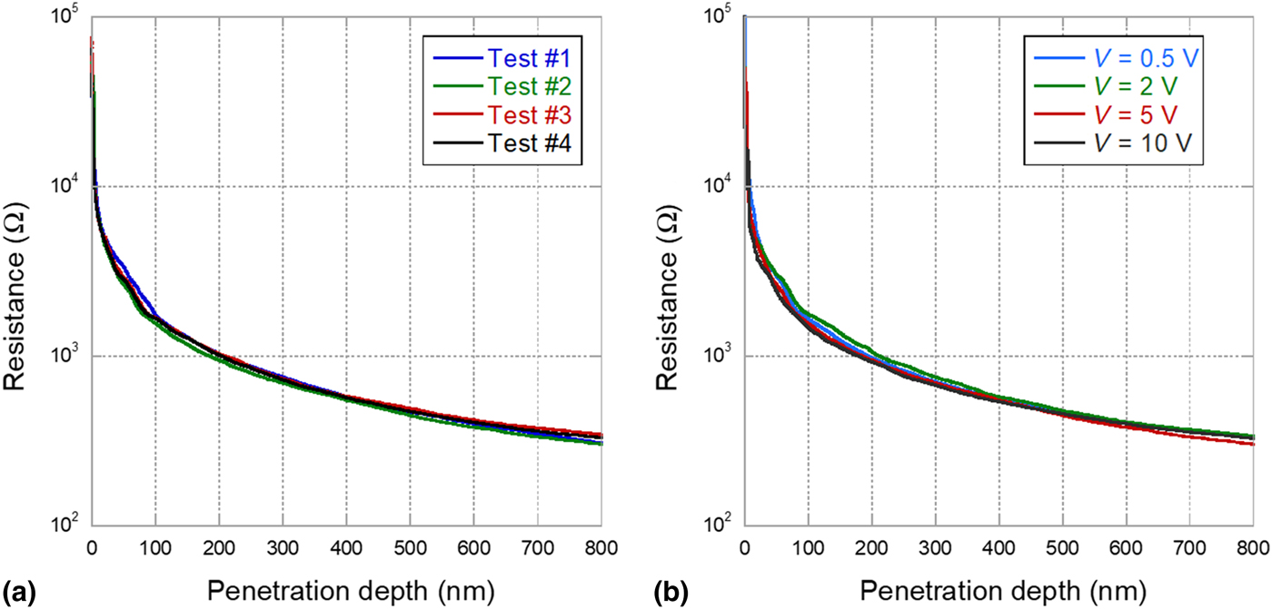
The resistance-versus-depth curves obtained during the indentation of the gold bulk sample on different spots are given in Fig. 1(a). This figure shows the high reproducibility of these experiments. As expected, the resistance continuously decreases as the mechanical contact area increases.[Reference Sprouster, Ruffel, Bradby, Stauffer, Major, Warren and Williams15] Figure 1(b) shows another set of resistive-nanoindentation tests performed at different polarization biases. One can notice that the resistance is bias-independent, which is the evidence of an ohmic-like electrical contact, in agreement with the absence of any interfacial layer between the tip and specimen.
Resistance evolution during indentation of the gold bulk single crystal. (a) Different tests performed at fixed polarization bias (5 V) and (b) performed at different polarization biases. <<color online>>.

Identification of resistance contributions
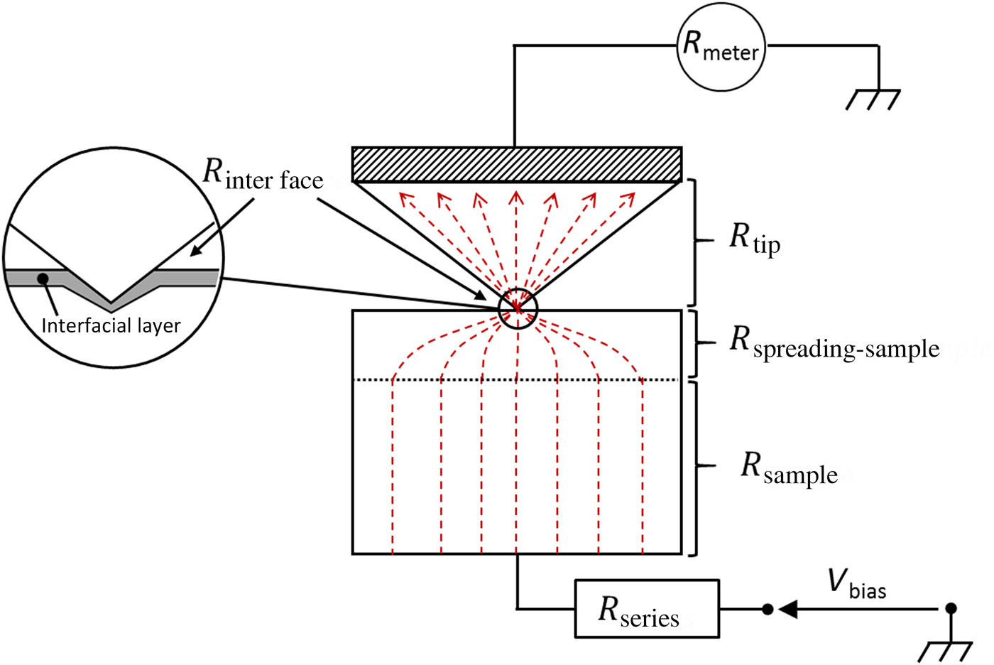
Before starting the procedure for the contact area computation, the different contributions to the measured resistance have to be identified. As long as the electronic transport between the BDD tip and the gold specimen remains in diffusive regime, the measured resistance is the sum of the following contributions (from top to bottom in Fig. 2):
i. The electrical resistance of the indentation tip (R tip);
ii. An interface resistance (R interface), coming from a possible interfacial layer;
iii. The spreading resistance within the sample (R spreading−sample), due to the current line constriction at the contact;
iv. The resistance from the gold sample (R sample);
v. An additional series resistance from the experimental set-up (R series).
Contributions to the measured resistance. Current lines are schematized by red-dotted lines.
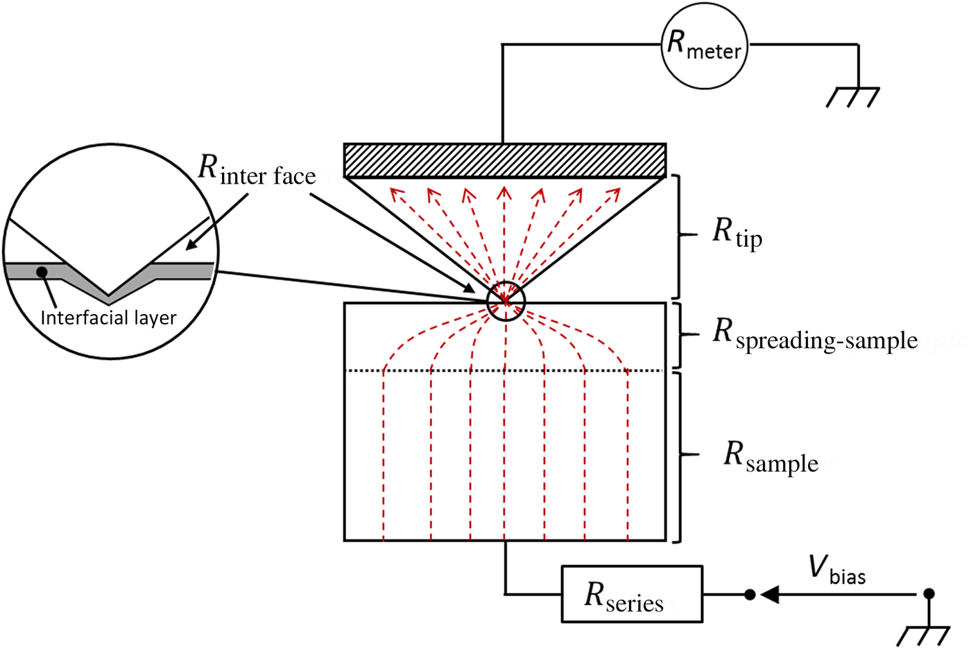
The two resistance contributions coming from the gold sample (R spreading−sample and R sample) depend linearly on its resistivity, similarly to the tip resistance (R tip) that depends linearly on the BDD tip resistivity. Since gold resistivity is at least five orders of magnitude lower than the BDD tip resistivity, R sample and R spreading−sample can be safely neglected. R interface can also be neglected, due to the absence of oxide or of another contaminant layer at the tip-to-sample interface. Consequently, the measured resistance R measured is simply the sum of the tip resistance and the additional constant series resistance:
 $$R_{{\rm measured}} = R_{{\rm series}} + R_{{\rm tip}}$$
The expression for R tip can be adapted from a model proposed by Schneegans et al. for the computation of a broken AFM tip[Reference Schneegans, Chrétien, Houzé and Meyer23]: the broken apex of the AFM tip is, in our case, the part of the indentation tip which has penetrated the sample [Supplementary Fig. S2(a)]. This consideration leads to Eq. (6) (with ρ tip the tip resistivity and α a constant related to the tip geometry):
 $$R_{{\rm tip}} = \alpha \cdot \displaystyle{{\rho _{{\rm tip}}} \over {h_{\rm c}}}$$
However, the experimental determination of h c is affected by the unavoidable tip defect (rounded apex of height h 0 [Supplementary Fig. S2(b)], thus Eq. (6) turns into Eq. (7):
 $$R_{{\rm tip}} = \alpha \cdot \displaystyle{{\rho _{{\rm tip}}} \over {h_{\rm c} + h_0}}$$
This expression relies on two strong assumptions: (1) the current distribution within the tip is homogeneous and parallel to the tip axis and (2) the part of the tip inside the sample affects only linearly the tip resistance.
Regarding the first assumption, it has been shown in the literature that the error arising from the use of a homogeneous and parallel distribution of current lines within the tip is <10%.[Reference Romano and Price24] The second assumption is more questionable. Since the BDD tip is five orders of magnitude more resistive than gold, current lines are expected to be localized at the periphery of the contact instead of being homogeneously distributed (Supplementary Fig. S3). This point has been confirmed by numerical computation (not shown). In literature, Nakamura et al.[Reference Nakamura25] have shown that the electrical resistance of ring contacts is equivalent to the resistance of the corresponding full-surface contact divided by a shape factor SF. This shape factor depends on the ratio between the ring thickness and the contact radius. For now, we first assume that this shape factor SF is constant during indentation (this assumption will be confirmed later).
Finally, the measured resistance is given by Eq. (8), where A and B indicate two constants that depend only on the experimental set-up (series resistance, tip geometry, and resistivity) but not on the specimen. These constants have to be determined experimentally during the calibration step (below), and will be further used for the effective nanoindentation measurements.
 $$R_{{\rm measured}} = A + \displaystyle{B \over {h_{\rm c} + h_0}}$$
Procedure for contact area computation
Now that these preliminary considerations have been stated, the step-by-step procedure for contact area computation can be described:
1. First the BDD tip geometry is determined. This step generates the tip “shape function” that relates the projected contact area to the contact depth.
2. An electrical calibration is carried out in order to determine the A and B constants [Eq. (8)]. As A and B depend only on the experimental set-up, a one-to-one analytical correspondence can be established between electrical resistance and contact depth (independently of the specimen).
3. The characterization of a conductive oxide-free specimen can thus be performed. Using the shape function (step 1), the contact area is finally determined from the contact depth values (step 2) for this specimen to be characterized.
Step 1. The determination of the tip geometry allows us to relate the total penetration depth H to the corresponding tip cross-section A. For that purpose, two complementary methods have been used: direct AFM imaging of the tip, and the calibration method described by Oliver and Pharr (where a model specimen with known isotropic elastic properties, like fused SiO2, is measured).[Reference Oliver and Pharr17] The obtained shape function can be simplified, leading to Eq. (9). The error due to this simplification is <5% for penetration depth larger than 45 nm.
 $$A_{\rm c} = \pi (\alpha _{{\rm tip}}(h_{\rm c} + h_0))^2;\;\alpha _{{\rm tip}} = 2.67;\;h_0 = 11.6\;{\rm nm}$$
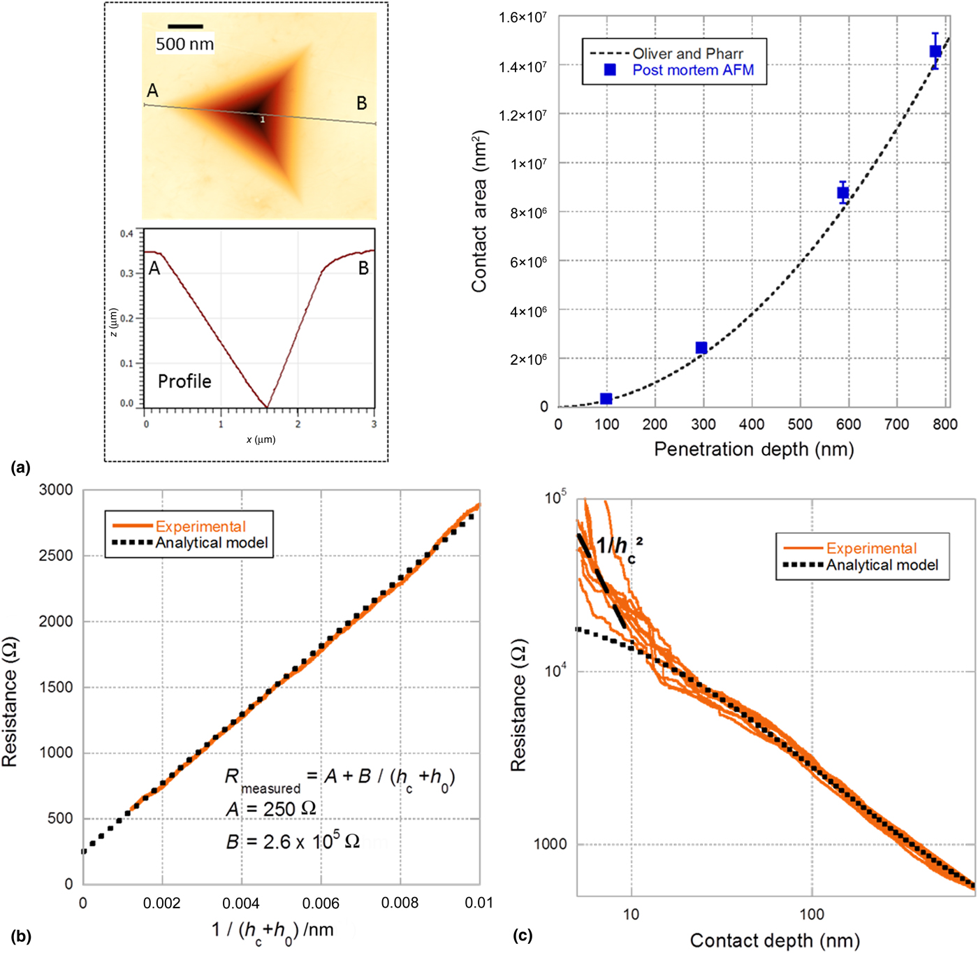
Step 2. In this work, electrical calibration has been performed on a gold bulk sample. Several resistive nanoindentation tests were run, up to different contact depths (circa 100, 300, 600 and 800 nm). Post-mortem AFM imaging shows that residual imprints exhibit sink-in, probably due to polishing-induced surface hardening [Fig. 3(a)]. Due to sink-in evidence, the contact depth can be reliably estimated from the Oliver and Pharr's model.[Reference Oliver and Pharr18] In order to validate the use of this model, the contact area was also computed from contact depth values, thanks to the tip “shape function” determined at step 1. The obtained contact area values were then compared to post-mortem AFM imaging, as shown in Fig. 3(a). This figure shows very good agreement between the estimated contact area using the Oliver and Pharr's model and the post-mortem AFM measurements. This step allows us to relate the total penetration depth to the contact depth.
Results from resistive-nanoindentation on the bulk gold sample. (a) Post-mortem AFM measures (left) and contact area against penetration depth (comparison of the Oliver–Pharr's model predictions to the post-mortem AFM measures, right). (b) Fitting of the resistance evolution against the reciprocal of the corrected contact height. (c) Resistance-versus-depth curves in logarithmic scales.

At this point, it is possible to plot the measured resistance R measured versus 1/(h c + h 0) [Fig. 3(b)] so that Eq. (8) can be fitted. The linear correlation (coefficient of 0.99) validates the proposed analytical expression of the measured resistance [Eq. (8)]. This linearity also validates the assumption of a constant shape factor SF during indentation. A and B constants are then obtained by simple linear fitting. Using these fitted values, both experimental and analytical resistance versus depth curves can be plotted [Fig. 3(c)]. Remarkably, a very good agreement is found between the experimental results and the analytical model for contact depths larger than 20 nm. Below these depths, the measured resistance is much higher than the model prediction. This deviation is most likely due to a change in electronic transport regimes from diffusive to ballistic since in ballistic regime, the electrical resistance evolves as  $1/h_{\rm c}^2 $.[Reference Sharvin26] This trend is in good agreement with that observed experimentally at small depths [Fig. 3(c)]. Alternatively, this deviation could also be explained by a multi-contact mode,[Reference Greenwood27] due to a potential thin interfacial layer at the contact.
Step 3. Once the entire analytical expression is fully set from the calibration sample, the specimen to be characterized can be processed: contact depth can then be directly determined from the resistance measurements. In the present work, this has been applied to a 200 nm polycrystalline gold thin film on a sapphire substrate. This sample has a complex rheology, as the film thickness acts as an additional length scale. The deformation field during nanoindentation is no more self-similar as in the bulk case. The standard practice to analyze such a soft-film-on-stiff-substrate structure is usually to determine the contact area by numerically solving a Fredholm integral[Reference Perriot and Barthel28] (or using finite elements simulations) coupled with at least one post-mortem measurement of the remaining imprints at a given depth (by SEM or AFM).
Experimental validation
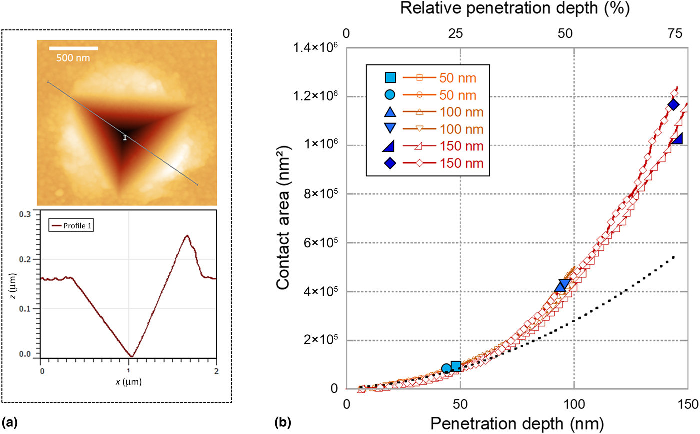
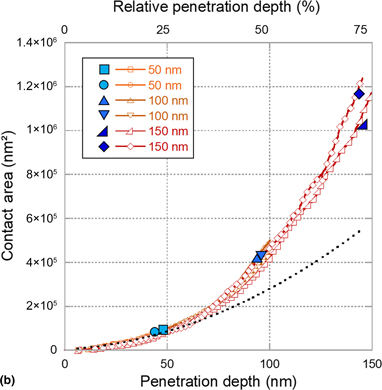
Resistive-nanoindentation tests with various final penetration depths were performed on this gold thin film. For each test, the contact depths were extracted continuously from resistance measurements [using Eq. (8)] and the corresponding contact areas were computed from the tip shape function [using Eq. (9)]. After each test, post-mortem AFM measurements were conducted for validation. Figure 4 reports the contact areas extracted from this procedure as well as post-mortem imaging data. An excellent agreement is observed, thus validating the whole methodology. It can be seen that the deformed film at a large relative penetration depth (75%) presents a large upheaval. At this depth, the contact area extracted from the Oliver–Pharr's method[Reference Oliver and Pharr18] (based on sink-in assumption) would be ~50% lower. The present procedure should apply to any specimen that satisfies the two following conditions: (1) the specimen is much more conductive than the indentation tip and (2) the specimen is oxide-free. The first condition is easily met for bulk metals, while the relevant magnitude is the sheet resistance for thin films. In the case of oxidized specimens, several potential solutions might be envisaged but require further assessments: application of large-enough voltages leading to dielectric breakdown, measurement under controlled environment (controlled relative humidity, submersion in liquids, etc.), tuning of applied voltages in accordance with the electrochemical potentials of the involved materials, etc.
Analysis of the resistive-nanoindentation tests on the 200 nm gold thin film. (a) Post-mortem AFM image and AFM profile showing evidence of pile-up. (b) Contact area against penetration depth: comparison of the data computed from the electrical measurements (open markers) and the corresponding post-mortem measurements (solid markers). Contact area from the Oliver and Pharr's model in a dotted line.

Conclusion
This paper reports an efficient method to extract the contact area during nanoindentation from resistance measurements. This method relies on three steps (tip shape measurement, set-up calibration, application to the specimen under test), and applies to oxide-free conductive materials. In the presence of an oxide layer, an additional non-linear contact resistance is expected, thus requiring the adaptation of the approach presented in this paper. Finally, the method is applied to nanoindentation tests performed on a sample with a complex rheology. The excellent agreement with the experimental area determination validates the proposed method. To our knowledge, this is the first time in literature that the contact area is extracted from electrical measurements during nanoindentation. It also paves the way for a new calibration procedure of both tip geometry and frame stiffness.
Supplementary material
The supplementary material for this article can be found at https://doi.org/10.1557/mrc.2019.74
Acknowledgments
This work has been performed with the financial support of the Centre of Excellence of Multifunctional Architectured Materials “CEMAM” n° ANR-10-LABX-44-01. The CEMAM program is funded by the French Agence Nationale de la Recherche (ANR). The authors thank the technical team of SIMaP lab (Bruno Mallery, Stéphane Massucci, and Nadine Vidal) for its support, as well as members of CSI/Scientec company (Les Ulis, France) for their support for the functionalization of the nanoindentation head: Louis Pacheco, Alan Lecoguiec, and Sylvain Poulet.