1. Introduction
The environmental issue of air pollution has forced the governments of many countries to implement more and more stringent regulations on vehicle emissions. This fact, along with high fuel costs, highlights the necessity and urgency of searching for new technologies to reduce aerodynamic drag and hence the fuel consumption of vehicles. The automobile industry has set an ambitious target to cut down the aerodynamic drag of vehicles by at least 30 % without compromising comfort, storage and the safety of passengers (Bruneau et al. Reference Bruneau, Creusé, Depeyras, Gilliéron and Mortazavi2011). As is typical for bluff bodies, the aerodynamic drag of a road vehicle is mainly due to pressure drag, which is strongly related to its wake (Hucho & Sovran Reference Hucho and Sovran1993). The development of successful drag reduction technologies calls for a thorough understanding of flow over a road vehicle.
Flow around a ground vehicle is highly three-dimensional and exhibits complex characteristics, such as flow separation and reattachment near the leading edge of the roof and side surface, the generation of coherent structures and the development of a turbulent boundary layer along the surface, and massive separation at the rear end (Choi, Lee & Park Reference Choi, Lee and Park2014). The generic geometry of a simplified car model provides a good reference for studying flow around a real vehicle. The Ahmed model is perhaps the most widely studied simplified vehicle model. Time-averaged experimental data (Ahmed, Ramm & Faltin Reference Ahmed, Ramm and Faltin1984; Lienhart, Stoots & Becker Reference Lienhart, Stoots and Becker2002; Lienhart & Becker Reference Lienhart and Becker2003) unveil three major coherent structures in the wake of this model, i.e. a separation bubble over the rear window, a pair of counter-rotating longitudinal or C-pillar vortices at the two side edges of the slanted surface, and two recirculation bubbles behind the vertical base. The aerodynamic drag is directly related to the interactions of these structures, which is governed by the slant angle φ. Two distinct flow regimes have been identified, divided by φ = 30° (Hucho & Sovran Reference Hucho and Sovran1993). At φ < 30°, the flow separates at the upper edge of the slanted surface and reattaches on the rear window, forming a separation bubble. C-pillar vortices are generated along the two side edges of the rear window. The size of the separation bubble and the strength of the C-pillar vortices both increase with increasing φ, and thus the drag rises rapidly to its maximum at φ = 30°. Beyond this φ, the C-pillar vortices burst and a fully separated flow develops above the rear window, resulting in a marked drag crash by about 31 % (Ahmed et al. Reference Ahmed, Ramm and Faltin1984).
The flow around a high-drag Ahmed model has been extensively investigated, including the flow structure around the front body (e.g. Spohn & Gilliéron Reference Spohn and Gilliéron2002), the wake topology (e.g. Krajnović & Davidson Reference Krajnović and Davidson2005a,Reference Krajnović and Davidsonb; Venning et al. Reference Venning, Lo Jacono, Burton, Thompson and Sheridan2017; Sellappan, McNally & Alvi Reference Sellappan, Mcnally and Alvi2018), the C-pillar vortices (e.g. Lehugeur, Gilliéron & Ta-Phuoc Reference Lehugeur, Gilliéron and Ta-Phuoc2005; Rouméas, Gilliéron & Kourta Reference Rouméas, Gilliéron and Kourta2009), and the instabilities and their predominant frequencies (e.g. Minguez, Pasquetti & Serre Reference Minguez, Pasquetti and Serre2008; Thacker et al. Reference Thacker, Aubrun, Leroy and Devinant2013; Tunay, Sahin & Ozbolat Reference Tunay, Sahin and Ozbolat2014; Tunay, Yaniktepe & Sahin Reference Tunay, Yaniktepe and Sahin2016). Zhang, Zhou & To (Reference Zhang, Zhou and To2015) conducted a rather comprehensive experimental study, largely focusing on unsteady flow structures around a high-drag Ahmed body of φ = 25° at Reynolds number  $Re \in [0.45,2.4] \times {10^5}$. Unless otherwise stated, Re and Strouhal number St are based on the square root of the model's frontal area A and free-stream velocity U∞. They found six distinct predominant frequencies over the rear window, behind the vertical base and above the roof, with St ranging from 0.14 to 2.12. The origin of every St was identified, reconciling the large scattering of St in previous reports. A rather complete conceptual flow structure model was proposed, embracing both steady and unsteady coherent structures around the body.
However, the flow around a low-drag Ahmed model has been less well understood than its high-drag body counterpart. A summary of previous experimental studies on the low-drag regime is given in table 1. These studies are mostly related to the steady characteristics of flow around an Ahmed model with φ = 35°. Lienhart et al. (Reference Lienhart, Stoots and Becker2002) and Lienhart & Becker (Reference Lienhart and Becker2003) investigated experimentally the time-averaged wake structure, as well as the surface pressure distribution on the rear window and vertical base (Re = 8.93 × 10⁵). A number of numerical investigations were launched for this flow at the same Re, focusing on comparison in the time-averaged flow fields between numerical and experimental results (Fares Reference Fares2006; Guilmineau Reference Guilmineau2008). Guilmineau et al. (Reference Guilmineau, Deng, Leroyer, Queutey, Visonneau and Wackers2017) studied numerically the flow around an Ahmed body with φ = 35° at Re = 8.93 × 10⁵ using the improved delayed detached-eddy simulation method. A small secondary recirculation at the end of the rear window was observed, which Lienhart & Becker (Reference Lienhart and Becker2003) failed to detect experimentally. Wang et al. (Reference Wang, Zhou, Pin and Chan2013) investigated the wake of an Ahmed body with φ = 35° based on extensive particle image velocimetry (PIV) measurements at Re = 0.62 × 10⁵. They found that the shear layer over the roof separated at the upper edge of the slant and was embedded with alternately signed longitudinal vortices. The separated flow merged into the upper recirculation behind the base. The gap flow separated from the lower edge of the base was partially drawn into the lower bubble, and partially rolled up to form a spanwise roll, which was wrapped by longitudinal structures. A conceptual flow structure model was proposed for the low-drag Ahmed body wake. However, this model fails to provide a full picture of the flow. Firstly, it is largely based on the mean flow data, containing little information on unsteady flow structure, let alone predominant frequencies in the wake. Secondly, some important details of the coherent structures are missing, including the development of longitudinal trailing vortices behind the vertical base.
Summary of experimental studies on the low-drag regime of an Ahmed body.

Unsteady structures around a low-drag Ahmed body and the corresponding St have received some attention. Kohri et al. (Reference Kohri, Yamanashi, Nasu, Hashizume and Katoh2014) measured the predominant frequencies in the wakes of Ahmed bodies with φ = 32.5° and 35° at Re = 0.73 × 10⁵ and captured three different St, i.e. St ≈ 0.10 in the symmetry plane behind the vertical base, 0.14 in the flow separated from the sidewall, and 0.27 downstream of the lower edge of the base. Tunay et al. (Reference Tunay, Sahin and Ozbolat2014) detected St = 0.26 in the downwash flow of the wake and 0.09 behind the lower edge of the base (φ = 35°, Re = 0.17 × 10⁵). Although the two frequencies are nearly the same as those (St ≈ 0.27 and 0.1) reported by Kohri et al. (Reference Kohri, Yamanashi, Nasu, Hashizume and Katoh2014), the two studies held different views on their mechanisms. Kohri et al. (Reference Kohri, Yamanashi, Nasu, Hashizume and Katoh2014) connected St ≈ 0.1 and 0.27 to the downwash flow from the slanted surface and the upwash flow from the lower edge of the base, respectively. But Tunay et al. (Reference Tunay, Sahin and Ozbolat2014) ascribed them to vortex shedding from the lower base edge and the upper edge of the rear window, respectively. Apparently, there is a need to clarify the St values as well as their origins. Furthermore, many other important issues remain to be resolved. For example, how do the unsteady structures interact with each other? What is the Re effect on the structures?
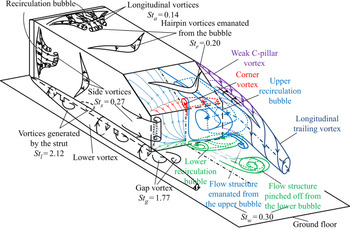
This work sets out to address the issues raised above based on extensive hot-wire, pressure, PIV and flow visualization measurements. Experimental details are provided in § 2. The predominant flow structures captured are presented in § 3, including their St values. The spatial extents of these structures or St values are discussed in § 4, followed by the examination of the Reynolds-number effect in § 5. A conceptual model of the flow structure around a low-drag Ahmed body is proposed in § 6. The work is concluded in § 7.
2. Experimental details
2.1. Experimental set-up
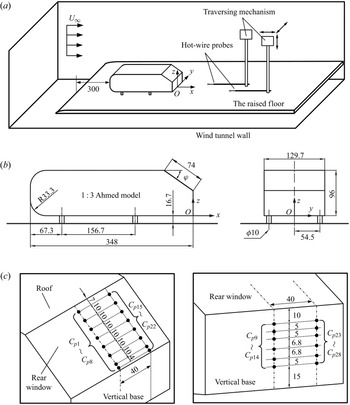
Experiments were carried out in two different closed-circuit wind tunnels, one at Harbin Institute of Technology, Shenzhen (HITsz), and the other at the Hong Kong Polytechnic University (HKPU), their working sections being 1.0 m × 0.8 m by 5.6 m long, and 0.6 m × 0.6 m by 2.4 m long, respectively. The flow non-uniformity was 0.1 % and the longitudinal turbulence intensity was no more than 0.4 % in the test section for both tunnels. The experimental set-ups were essentially the same, as shown schematically in figure 1(a). A flat plate with a clipper-built leading edge was installed horizontally above the floor of the test section, as a raised floor to control the boundary layer thickness. The dimensions of the plates were 2.6 m × 0.78 m × 0.015 m and 2.2 m × 0.59 m × 0.015 m, with clearances between the plate and the tunnel floor of 0.275 m and 0.088 m, in the HITsz and HKPU wind tunnels, respectively.
(a) Schematic of the experimental arrangement. (b) Dimensions of a one-third-scaled Ahmed body (35°). (c) Pressure tap distribution on the rear end. The length unit is millimetre.

The vehicle model was a one-third-scaled Ahmed body (figure 1b) with φ = 35°, corresponding to a low-drag body. The full-scale model was described by Ahmed et al. (Reference Ahmed, Ramm and Faltin1984). The model had an overall length of L = 0.348 m, a width of W = 0.130 m and a height of H = 0.096 m, supported by four cylindrical struts of 16.67 mm in length and 10 mm in diameter. The front end of the model was 0.3 m downstream of the floor leading edge (figure 1a), where the boundary layer thickness was about 4 mm at  ${U_\infty } = 8.33\;\textrm{m}\;{\textrm{s}^{ - 1}}$ or Re = 0.62 × 10⁵. The blockage ratios of the frontal surface of the model to the rectangular test section above the raised floor were approximately 2.2 % and 4.1 % in the HITsz and HKPU wind tunnels, respectively. Figure 1(b) shows the definition of the right-handed Cartesian coordinate system (x, y, z), with the origin O at the midpoint of the lower edge of the model vertical base. In this paper, the instantaneous velocity components in the x, y and z directions are defined as U, V and W, respectively, which can be decomposed into a time-averaged component and a fluctuating component, i.e.
 $U = \bar{U} + u$,
 $V = \bar{V} + v$ and
 $W = \bar{W} + w$, where overbar denotes time averaging and u, v and w are fluctuating velocities.
2.2. Measurement techniques
Single hot-wire probes fixed on a computer-controlled Dantec traverse system were used at HKPU to measure u for the estimate of the predominant frequencies in the flow (figure 1a). The sensing element was a tungsten wire of 5 μm diameter and about 1 mm in length. The wire was operated on a constant-temperature circuit (Dantec Streamline) at an overheat ratio of 1.8. The signal from the wire was offset, amplified, low-pass filtered at a cut-off frequency of 1.0 kHz, and digitized at a sampling frequency fs of 3.0 kHz using a 16-bit analogue-to-digital converter (NI PCI-6143). The sampling duration was 3 min for each record. At least three records were collected for each measurement location. Flow is assumed to be symmetric with respect to the plane y* = 0, where superscript ‘*’ denotes normalization by  $\sqrt A \textrm{ }( = 0.112\;\textrm{m})$ and/or U∞. Therefore, the hot-wire measurements were performed only on the side of y* ≥ 0, covering the regions of x* = −1.27, y* ∈ [0, 0.43] and z* ∈ [0.91, 1.17] above the roof, x* = −1.27, y* ∈ [0.63, 0.69] and z* ∈ [−0.04, 0.90] over the side surface, x* ∈ [−0.54, 0], y* ∈ [0, 0.57] and z* ∈ [0.59, 0.91] over the rear window, and x* ∈ [0.09, 1.52], y* ∈ [0, 0.72] and z* ∈ [−0.04, 0.90] behind the vertical base. The total measurement points amount to more than 1500. The fast Fourier transform (FFT) algorithm was employed to calculate the power spectral density function Eu of u. The FFT window size Nw was 4096. The frequency resolution Δf in the spectral analysis depends on the sampling frequency and the FFT window size (Δf = fs/Nw) and is estimated to be 0.73 Hz (Zhou et al. Reference Zhou, Du, Mi and Wang2012).
A Dantec high-speed two-dimensional PIV system (Litron LDY304-PIV, Nd:YLF) was used at the HITsz wind tunnel to measure the wake of the Ahmed body. The model surface and raised floor were painted black to minimize laser reflection noise. The flow was seeded by smoke generated from peanut oil using a TSI 9307-6 particle generator, with particles of about 1 μm in diameter. Flow illumination was provided by two pulsed laser sources of a 527 nm wavelength, each with a maximum energy output of 30 mJ pulse−1. Particle images were taken using a charge-coupled device camera (PhantomV641, double frames, with a resolution of 2560 × 1600 pixels). Synchronization between image taking and flow illumination was provided by a Dantec timer box 80N77. PIV measurements were performed in four x–z planes of y* = 0, 0.14, 0.36 and 0.54, and eight y–z planes, i.e. x* = −1.27 at the roof and side surface of the body, x* = −0.36 and −0.09 above the rear window, and x* = 0.20, 0.43, 0.65, 0.86 and 1.29 behind the base. The PIV image covered an area of x* ∈ [−0.88, 2.80] and z* ∈ [−0.30, 1.99] for the x–z planes and y* ∈ [−0.60, 0.98] and z* ∈ [−0.35, 2.17] for the y–z planes. The image magnifications in both directions of each plane were identical, approximately 160 and 110 μm pixel−1 in the x–z and y–z planes, respectively. The intervals between two successive pulses were 120 μs and 40 μs for measurements in the x–z and y–z planes, respectively. In processing PIV images, the adaptive PIV method (Dynamic Studio software) was used with a minimum interrogation area size of 32 × 32 pixels and a maximum size of 64 × 64 pixels. The number of particle densities per interrogation window was at least 25 or 20 in the x–z or y–z planes, respectively. The grid step size of 16 × 16 pixels produced 160 × 100 in-plane velocity vectors and the same number of vorticity data in the x–z and y–z planes.
Following Zhang et al. (Reference Zhang, Liu, Zhou, To and Tu2018), the uncertainty of PIV measurements was estimated based on image matching analysis. This method identifies particle image pairs in two successive exposures according to the measured displacement vectors and evaluates the residual distance or particle disparity vector between the particle image pairs, whose ensemble within the interrogation window is used to infer the instantaneous uncertainty of the measured displacement. For further details of this technique, please refer to Sciacchitano, Wieneke & Scarano (Reference Sciacchitano, Wieneke and Scarano2013). In the x–z planes, the estimated particle displacement uncertainties are below 0.15 pixels in both x and z directions, resulting in velocity uncertainties σU and σW, in U and W, less than 0.2 m s−1 or 2.5 % of U∞, respectively. Following Wen, Tang & Duan (Reference Wen, Tang and Duan2015), the uncertainty σωy of the spanwise vorticity ωy is given by
 \begin{equation}{\sigma _{\omega y}} = {\sigma _U}/\mathrm{\Delta }x,\end{equation}
where Δx is the grid size (16 pixels). Therefore, the σωy is less than 7 % of the highest magnitude of ωy (about 1100–1500 s−1) in the x–z planes of y* ∈ [0, 0.54]. In the y–z planes of x* ∈ [−1.27, 1.29], the estimated particle displacement uncertainties are below 0.1 pixels in both y and z directions, accounting for velocity uncertainties of less than 3.3 % of U∞ in both V and W. The uncertainty σωx of the streamwise vorticity ωx is less than 16 % of the highest magnitude of ωx (about 900–1350 s−1) in the y–z planes of x* ∈ [−1.27, 1.29].
PIV measurements were conducted twice with two different trigger rates in each plane. A lower trigger rate of 200 Hz was used for time averaging in order to obtain data with a longer time period. The other is set at 500 Hz to achieve a higher temporal resolution for instantaneous and proper orthogonal decomposition (POD) analyses. A total of 2000 PIV images were captured in the double frame mode for each test run. The percentage variations of all mean and root mean square velocities  ${\bar{U}^\ast },{\bar{V}^\ast },{\bar{W}^\ast }$,
 $u_{rms}^\ast ,v_{rms}^\ast $ or
 $w_{rms}^\ast $ converge with increasing N to less than ±1 % once N > 1500, irrespective of the measurement plane or trigger rate. As such, N = 2000 is considered to be adequate for capturing the mean and fluctuating flow fields.
Laser-induced fluorescence (LIF) flow visualization was conducted at HKPU using a Dantec standard PIV system (PIV2100). Please refer to Zhang et al. (Reference Zhang, Zhou and To2015) for the details of the experimental set-up. Three rows of pinholes, each consisting of 64 circular orifices, 1 mm in diameter and equally separated by 1 mm, were made along lines parallel to and 7 mm upstream of the upper edge of the rear window, and the upper and lower edges of the vertical base, respectively. Smoke generated by a TSI 3079 particle generator using paraffin oil was pumped through one hollow cylindrical strut into a cavity in the rear part of the model and released into the flow from the pinholes. Flow images were taken in the x–z plane of y* = 0 and the x–y plane of z* = 0.72 over the rear window. The model surface, the raised floor and the tunnel working section walls hit by the laser sheets were all painted black to minimize reflection.
A PSI DTC Initium system was used to measure the time-averaged surface pressure on the model at HITsz. Twenty-eight pressure taps were made, whose locations are schematically shown in figure 1(c). The pressure taps were connected to an ESP scanner via plastic tubes of 1 mm inner diameter. The scanner was placed inside the test model to minimize the length of the tubes and hence the filtering effect of tubing in pressure measurements (Grandemange, Gohlke & Cadot Reference Grandemange, Gohlke and Cadot2013). The measurement accuracy was estimated to be approximately ± 2 Pa. The sampling frequency was 650 Hz, and a total of 40 000 data points were obtained for each measurement location. The time-averaged pressure coefficient is given by  ${C_p} = (p - {p_0})/(0.5\rho U_\infty ^2)$, where p and p 0 are the time-averaged local and free-stream static pressures, respectively, and ρ is the density of air.
The hot-wire and flow visualization measurements were carried out at  ${U_\infty } \in [4,36]\;\textrm{m}\;{\textrm{s}^{ - 1}}$ and 3 m s−1, corresponding to Re ∈ [0.3, 2.7] × 105 and 0.22 × 10⁵, respectively. The PIV and pressure measurements were performed at
 ${U_\infty } = 8.3\;\textrm{m}\;{\textrm{s}^{ - 1}}$ (Re = 0.62 × 10⁵). The U∞ value was measured using a Pitot-static tube connected to an electronic micro-manometer (Furness Control Ltd, FC510). Note that the Ahmed model has sharp edges at the rear end, and the flow structure at this relatively low Re range does not differ significantly from that at large Re of the order of 106 (Vino et al. Reference Vino, Watkins, Mousley, Watmuff and Prasad2005).
3. Predominant flow structures
3.1. Recirculation bubbles
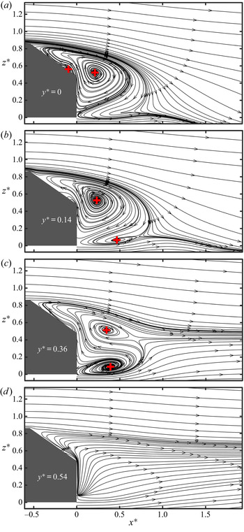
Time-averaged streamlines in the x–z planes of y* = 0, 0.14, 0.36 and 0.54 (figure 2) show that the flow separates at the upper edge of the rear window and the lower edge of the vertical base, and rolls up behind the base, forming two recirculation bubbles, one above the other. The centre of the upper bubble is located at x* = 0.22 and z* = 0.52 near the symmetry plane (figure 2a,b), and deviates slightly from Tunay et al.'s (Reference Tunay, Sahin and Ozbolat2014) observation (x* = 0.26 and z* = 0.6), also from PIV measurements, in the symmetry plane (φ = 35°, Re = 0.17 × 10⁵). This deviation is not unexpected in view of differences in facilities, techniques, Re, etc., between the two experiments. In the x–z plane of y* = 0.36, the centre moves downstream to (x*, z*) = (0.35, 0.51) (figure 2c), suggesting that the upper bubble centre is tilted downstream from the symmetry plane to the off-symmetry plane. On the other hand, the centre of the lower bubble shifts upstream, from (x*, z*) = (0.47, 0.07) to (0.39, 0.09), from the plane of y* = 0.14 to that of y* = 0.36. In the x–z plane of y* = 0.54, both bubbles disappear (figure 2d), and an upwash flow occurs over the rear window and behind the base.
PIV-measured time-averaged sectional streamlines in x–z planes of (a) y* = 0, (b) y* = 0.14, (c) y* = 0.36 and (d) y* = 0.54 at Re = 0.62 × 10⁵. The red ‘+’ denotes the focus of streamlines.

The vortex definition proposed by Zhou et al. (Reference Zhou, Adrian, Balachandar and Kendall1999) is presently adopted for the identification of vortices from the vorticity data and is briefly introduced below. A vortex core is a region where the velocity gradient tensor  $\boldsymbol{\nabla }\boldsymbol{U}$ has complex eigenvalues (Chong, Perry & Cantwell Reference Chong, Perry and Cantwell1990). Then,
 $\boldsymbol{\nabla }\boldsymbol{U}$ may be written as
 \begin{equation}\boldsymbol{\nabla }\boldsymbol{U}\; = [\begin{array}{@{}ccc@{}} {{\boldsymbol{v}_r}}&{{\boldsymbol{v}_{cr}}}&{{\boldsymbol{v}_{ci}}} \end{array}]\left[ {\begin{array}{@{}ccc@{}} {{\lambda_r}}&{}&{}\\ {}&{{\lambda_{cr}}}&{{\lambda_{ci}}}\\ {}&{ - {\lambda_{ci}}}&{ - {\lambda_{cr}}} \end{array}} \right]{[\begin{array}{@{}ccc@{}} {{\boldsymbol{v}_r}}&{{\boldsymbol{v}_{cr}}}&{{\boldsymbol{v}_{ci}}} \end{array}]^{ - 1}},\end{equation}
where λr is the real eigenvalue with a corresponding eigenvector vr, and λcr ± λcii are a conjugate pair of complex eigenvalues with complex eigenvectors vcr ± vcii. The local flow is either stretched or compressed along the axis vr, while swirling in the plane spanned by vectors vcr and vci. The strength of the local swirling motion is quantified by the imaginary part of the complex eigenvalue pair λci, referred to as the local swirling strength of the vortex. This method is frame-independent and does not detect regions containing significant vorticity but no local swirling motion, such as shear layers. A vortex is identified if  $\lambda _{ci}^{2\ast }$ is larger than a threshold, 0.4 in the x–z planes and 0.002 in the y–z planes, which are about 3 % and 1 % of the maximum
 $\lambda _{ci}^{2\ast }$, respectively.
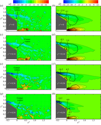
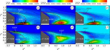
As shown in the contours of instantaneous spanwise vorticity  $\omega _y^\ast $ in each x–z plane from y* = 0 to 0.54 (figure 3a,c,e,g), one highly concentrated negative (or positive) vorticity layer separates from the upper edge of the rear window and another from the lower edge of the base. The former in the plane of y* = 0.54 (figure 3g) is deflected downwards towards the surface, as compared with its counterpart in the symmetry plane (figure 3a), spatially coinciding with the well-known C-pillar vortex. The wake is characterized by two regions, the upper of the negative
 $\omega _y^\ast $ concentrations and the lower of the positive, and the two regions appear contracting from y* = 0 to 0.54. This contraction is confirmed by the
 $\bar{\omega }_y^\ast $ contours (figure 3b,d,f,h) and is internally consistent with the streamlines (figure 2), where both bubbles are even invisible in the plane of y* = 0.54 (figure 2d).
PIV-measured typical instantaneous (a,c,e,g) and time-averaged (b,d,f,h) spanwise vorticity contours in x–z planes of (a,b) y* = 0, (c,d) y* = 0.14, (e,f) y* = 0.36 and (g,h) y* = 0.54 at Re = 0.62 × 10⁵. Black thick lines are contours of the swirling strength  $\bar{\lambda }_{ci}^{2\ast } = 0.4$ of the time-averaged flow. The magnitudes of
 $\bar{\omega }_{y,max}^\ast $ and
 $\bar{\omega }_{y,min}^\ast $ are marked in the figure.

Interestingly, a small corner vortex with positive vorticity occurs at the lower end of the rear window, which runs across almost the entire width of the window with  $\bar{\omega }_{y,max}^\ast\approx 4.0$. In this paper, subscripts ‘max’ and ‘min’ denote extreme values in positively and negatively signed vorticity concentrations, respectively. Wang et al. (Reference Wang, Zhou, Pin and Chan2013) captured a similar structure based on the PIV measurements in the x–z plane of y* = 0 behind an Ahmed body (φ = 35°, Re = 0.62 × 10⁵), and suggested that this structure was induced by the negative circulation above the rear window. No further discussion was pursued. In the present work, a different view on the formation of the corner vortex, as well as its effect on the surface pressure, is provided based on the PIV, pressure and flow visualization data.
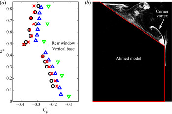
The time-averaged pressure coefficient Cp on the rear window (figure 4a) drops gradually downstream from Cp 1 = −0.32 at z* = 0.82 to Cp 8 = −0.38 at z* = 0.50 in the symmetry plane of y* = 0. On the other hand, Cp on the vertical base increases almost linearly from Cp 9 = −0.27 at z* = 0.39 to Cp 14 = −0.18 at z* = 0.13. Similar observations have been made from Cp 15 to Cp 28 in the off-symmetry plane of y* = 0.36. The Cp distribution is in reasonable agreement with previous measurements on the rear end of an Ahmed body with φ = 35° by Lienhart & Becker (Reference Lienhart and Becker2003) and Meile et al. (Reference Meile, Ladinek, Brenn, Reppenhagen and Fuchs2016). There is an appreciable deviation in Cp, which is ascribed to the differences in experimental conditions such as Re and facilities among these studies. The pressure on the vertical base is appreciably higher than that on the rear window. The flow within the upper recirculation bubble near the vertical base moves upwards along the base under the pressure gradient, which is evident in figure 3. Such upward-moving fluid separates at the upper edge of the base and then rolls up before reattachment on the slanted surface under the pressure difference between the two surfaces, forming the corner vortex, which is very well illustrated by one typical photograph captured from flow visualization in the symmetry plane (figure 4b).
(a) Time-averaged pressure coefficients Cp on the rear end in the symmetry plane of y* = 0 (red ‘×’) and an off-symmetry plane of y* = 0.36 (black ‘○’) at Re = 0.62 × 10⁵. The blue ‘ $\Delta$’ and green ‘
 $\nabla$’ symbols denote Cp experimentally obtained in the plane of y* = 0 by Lienhart & Becker (Reference Lienhart and Becker2003) (Re = 8.93 × 10⁵) and Meile et al. (Reference Meile, Ladinek, Brenn, Reppenhagen and Fuchs2016) (Re = 6.70 × 10⁵), respectively, for an Ahmed body with φ = 35°. (b) A typical photograph of the flow structure in the symmetry plane at Re = 0.22 × 10⁵. Flow is from left to right.

Grandemange et al. (Reference Grandemange, Gohlke and Cadot2013) observed a bistability in the wake of a square-back Ahmed body, which is characterized by random spanwise switchings of the recirculation region between two preferred reflectional symmetry-breaking positions. The same observation was also made and investigated by Östh et al. (Reference Östh, Noack, Krajnović, Barros and Borée2014) and Barros et al. (Reference Barros, Borée, Cadot, Spohn and Noack2017). This phenomenon has, however, never been observed in the wake of the low-drag regime.
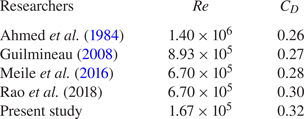
The measured time-averaged drag coefficient  ${C_D}\textrm{ }({\equiv} {F_D}/(0.5\rho U_\infty ^2A)$, where FD is aerodynamic drag) is 0.32, slightly higher than previous reports by Ahmed et al. (Reference Ahmed, Ramm and Faltin1984), Guilmineau (Reference Guilmineau2008), Meile et al. (Reference Meile, Ladinek, Brenn, Reppenhagen and Fuchs2016) and Rao et al. (Reference Rao, Minelli, Basara and Krajnović2018), which is probably due to the present lower Re. It is evident in table 2 that CD decreases from 0.32 to 0.26 from Re = 1.67 × 10⁵ to 1.4 × 10⁶.
Drag coefficient CD on an Ahmed body with φ = 35°.

3.2. Longitudinal structures
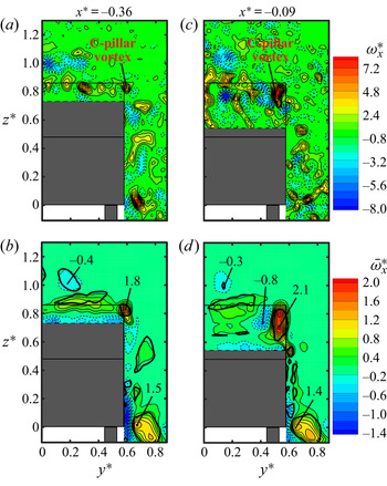
Figure 5 presents the PIV-measured instantaneous and time-averaged streamwise vorticities in the y–z planes. At x* = −0.36, a streamwise vortex with positive  $\omega _x^\ast $ is captured near the upper corner of the rear window (figure 5a), accounting for a swirling motion as enclosed by the swirling strength
 $\bar{\lambda }_{ci}^{2\ast } = 0.002$ of the time-averaged flow with
 $\bar{\omega }_{x,max}^\ast{=} 1.8$ (figure 5b). This swirling region grows larger and the corresponding
 $\bar{\omega }_{x,max}^\ast $ increases to 2.1 downstream in the plane of x* = −0.09 (figure 5d). This longitudinal structure is apparently the C-pillar vortex, which is formed due to the rollup of the shear layer coming off the sidewall about the side edge of the rear window because of the pressure difference between the flows over the sidewall and the slanted surface (Ahmed et al. Reference Ahmed, Ramm and Faltin1984). The strength of the C-pillar vortex is substantially lower than that in the high-drag regime; its
 $\bar{\omega }_{x,max}^\ast $ in the y–z plane of x* = 0.20 was only about 10 % of the latter (Wang et al. Reference Wang, Zhou, Pin and Chan2013). It is noteworthy that the
 $\bar{\omega }_{x,max}^\ast $ location of the C-pillar vortex moves inwards and downwards from (y*, z*) = (0.59, 0.82) at x* = −0.36 to (0.53, 0.70) at x* = −0.09. Its angles are about 11° and 12° with respect to the slanted surface and the sidewall, respectively, larger than those (8° and 7°) at φ = 25° (Lehugeur et al. Reference Lehugeur, Gilliéron and Ta-Phuoc2005).
PIV-measured instantaneous (a,c) and time-averaged (b,d) streamwise vorticity contours in the y–z planes of x* = −0.36 (a,b) and x* = −0.09 (c,d) at Re = 0.62 × 10⁵. The thick black curves are the contours of the swirling strength  $\bar{\lambda }_{ci}^{2\ast } = 0.002$ of the time-averaged flow. The magnitudes of
 $\bar{\omega }_{x,max}^\ast $ and
 $\bar{\omega }_{x,min}^\ast $ are marked in the figure.

As shown in the  $\bar{\omega }_x^\ast $ contours in the y–z plane of x* = −0.09 (figure 5d), a relatively strong
 $\bar{\omega }_x^\ast $ concentration is present in the vicinity of the C-pillar vortex, whose sign is opposite to that of the C-pillar vortex, with
 $\bar{\omega }_{x,min}^\ast $ reaching −0.8, though without swirling. This vorticity concentration is induced by the C-pillar vortex (Zhang et al. Reference Zhang, Zhou and To2015). A number of alternately signed
 $\omega _x^\ast $ concentrations are discernible at the same height as the roof in the y–z planes of x* = −0.36 and −0.09 (figure 5a,c), which are probably associated with the hairpin vortices wrapped with the longitudinal vortices above the roof. There is another streamwise swirling structure enclosed by the contour of
 $\bar{\lambda }_{ci}^{2\ast } = 0.002$ near the lower corner of the sidewall in both planes. This structure, referred to as the lower vortex, is formed along the lower edge of the sidewall (Wang et al. Reference Wang, Zhou, Pin and Chan2013).
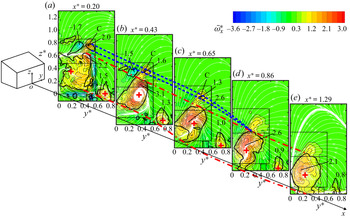
It is insightful to examine the  $\bar{\omega }_x^\ast $ contours, superimposed with sectional streamlines, in different y–z planes behind the vertical base (figure 6). At x* = 0.20 (figure 6a), the upper rightmost concentration marked by ‘C’ may be identified with the C-pillar vortex. Apparently, the C-pillar vortex starts to decay from
 $\bar{\omega }_{x,max}^\ast{=} 2.0$ to 1.3 from x* = 0.20 to 0.65 (figure 6a–c). A longitudinal swirling structure (marked by the contour of
 $\bar{\lambda }_{ci}^{2\ast } = 0.002$) with
 $\bar{\omega }_{x,min}^\ast{=}{-} 1.7$ occurs in x* = 0.20 on the inner side, close to the symmetry plane, of the C-pillar vortex, probably resulting from the interaction between the C-pillar vortex and the upper recirculation bubble. This induced structure starts to decay downstream with the C-pillar vortex. Behind the base, there is a large swirling structure enclosed by the contour of
 $\bar{\lambda }_{ci}^{2\ast } = 0.002$ (figure 6a), which coincides spatially with the upper bubble. Its vorticity concentration increases from
 $\bar{\omega }_{x,max}^\ast{=} 2.2$ at (y*, z*) = (0.45, 0.58) in the y–z plane of x* = 0.20 to
 $\bar{\omega }_{x,max}^\ast{=} 3.1$ at (y*, z*) = (0.38, 0.52) in the plane of x* = 0.43 (figure 6a,b). In both planes, the
 $\bar{\omega }_{x,max}^\ast $ value occurs at almost the same height (z* ≈ 0.52) as the upper bubble centre (figure 2). When moving downstream to x* = 0.65,
 $\bar{\omega }_{x,max}^\ast $ drops to 2.6 (figure 6c). Based on the streamlines in the x–z planes of y* ∈ [0, 0.36] (figure 2a–c), this longitudinal structure is linked to the upper bubble, which runs laterally outwards downstream. This longitudinally tilted large structure induces an upwash flow on its outer side (figure 6a–c), responsible for the upwash captured in the x–z plane of y* = 0.54 (figure 2d), and a downwash flow on the inner side close to the symmetry plane (figure 6b,c). Both the C-pillar vortex and the large longitudinal structure move downwards and towards the symmetry plane from x* = 0.43 to 0.65 (figure 6b,c) under a pressure difference between the outer flow and the wake. From x* = 0.86, the C-pillar vortex appears to merge into the longitudinal large structure (figure 6d,e), that is, the far wake is dominated by one single pair of longitudinal trailing vortices. The lower vortex (figure 5) decays gradually in the wake from
 $\bar{\omega }_{x,max}^\ast{=} 1.5$ at x* = 0.20 to
 $\bar{\omega }_{x,max}^\ast{=} 0.8$ at x* = 1.29 (figure 6).
Downstream evolution of PIV-measured time-averaged streamwise vorticity contours and sectional streamlines in y–z planes (Re = 0.62 × 10⁵). The red ‘+’ and the thick black curves are as in figures 2 and 5, respectively. The blue broken lines and red dashed-dotted lines are indicative for the upper and lower borders of the swirling regions corresponding to the C-pillar vortex and the leg of the upper recirculation bubble, respectively. The magnitudes of  $\bar{\omega }_{x,max}^\ast $ and
 $\bar{\omega }_{x,min}^\ast $ are marked in the figure.

3.3. Unsteady wake vortices and scaling
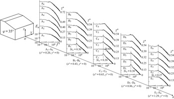
Unsteady flow structures behind the base are investigated via Eu measured at different heights in the symmetry plane for a number of downstream stations (figure 7). There is no prominent peak in Eu measured at x* = 0.2 over the range of z* ∈ [0, 0.72]. A rather pronounced peak occurs at f* = Stw = 0.30 at B1 (z* = 0) and B3 (z* = 0.25) at x* = 0.43, C1 (z* = 0), C3 (z* = 0.25) and C4 (z* = 0.32) at x* = 0.65, and D1 (z* = 0) and D3 (z* = 0.25) at x* = 0.86, but not at B2, C2 and D2 (z* = 0.13), where a minor peak is discernible only at the second harmonic of Stw = 0.30, i.e. f* = 0.60. The peak at Stw = 0.30 becomes more pronounced with increasing x* for lower positions B1 through D1 and more visible at higher z* (B3, z* = 0.25; C4, z* = 0.32) from x* = 0.43 to 0.65. The observations suggest that the unsteady structures associated with Stw = 0.30 are related to the two recirculation bubbles behind the base. The peak at Stw = 0.30 is no longer visible for x* ≥ 1.29, suggesting the disappearance of these unsteady structures.
Power spectral density function Eu of the hot-wire signal measured along A1–A6, B1–B6, C1–C6, D1–D6 and E1–E6, respectively, at y* = 0 in the wake, at Re = 0.62 × 10⁵.

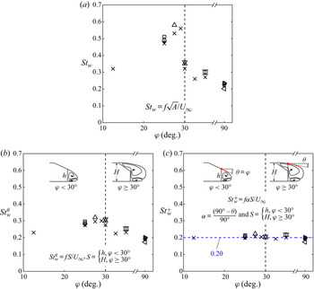
Zhang et al. (Reference Zhang, Zhou and To2015) captured a predominant frequency of Stw = 0.44, larger than the present Stw, behind the vertical base of an Ahmed model with φ = 25° (Re = 0.62 × 10⁵). Other investigators (e.g. Minguez et al. Reference Minguez, Pasquetti and Serre2008; Joseph, Amandolese & Aider Reference Joseph, Amandolese and Aider2012; Kohri et al. Reference Kohri, Yamanashi, Nasu, Hashizume and Katoh2014) also reported this predominant frequency, varying rather wildly, in the wake of an Ahmed body with various φ (figure 8a). One may wonder whether there is any scaling law to govern this predominant frequency. In the high-drag regime, the flow separates from both the upper and lower edges of the base, forming two recirculation bubbles behind the base. The Stw is attributed to the alternate emanation of unsteady structures from the two bubbles (Zhang et al. Reference Zhang, Zhou and To2015). We may surmise that the height h of the vertical base is a characteristic length in this case. On the other hand, H might be the characteristic length in the low-drag regime where the two recirculation bubbles result from flow separation from the upper edge of the rear window and the lower edge of the base. Note that the Ahmed body with the critical angle φ = 30° can be in either high- or low-drag regimes (Sims-Williams Reference Sims-Williams2001; Conan, Anthoine & Planquart Reference Conan, Anthoine and Planquart2011; Kohri et al. Reference Kohri, Yamanashi, Nasu, Hashizume and Katoh2014). Furthermore, it was observed even in the high-drag regime that the separated flow over the rear window did not fully reattach on the slanted surface and, instead, merged with the upper bubble behind the base (Vino et al. Reference Vino, Watkins, Mousley, Watmuff and Prasad2005; Conan et al. Reference Conan, Anthoine and Planquart2011). That is, H should be considered as the characteristic length for φ = 30° in both regimes. As such, we may define
 \begin{equation}St_w^{\#} = fS/{U_\infty },\quad S = \left\{ {\begin{array}{@{}ll} {h,}&{\varphi \; \lt \; 30^\circ ,}\\ {H,}&{\varphi \; \ge \; 30^\circ ,} \end{array}} \right.\end{equation}
where S is the vertical distance between the separation points of the two bubbles. The square-back Ahmed body may be described by φ = 0° or 90°, corresponding to S = h or H, respectively, where h equals H.
Dependences of (a) Stw, (b)  $St_w^{\#} $ and (c)
 $St_w^ + $ on φ. Symbols: ○, present measurement (Re = 0.62 × 10⁵); ×, Kohri et al. (Reference Kohri, Yamanashi, Nasu, Hashizume and Katoh2014, Re = 0.73 × 10⁵); +, Zhang et al. (Reference Zhang, Zhou and To2015, Re = 0.89 × 10⁵); Δ, Sims-Williams (Reference Sims-Williams2001, Re ∈ [3.10, 6.40] × 105); ∇, Vino et al. (Reference Vino, Watkins, Mousley, Watmuff and Prasad2005, Re = 4.40 × 10⁵);
 ${\triangleleft} $, Grandemange et al. (Reference Grandemange, Gohlke and Cadot2013, Re = 1.07 × 10⁵);
 ${\triangleright} $, Barros et al. (Reference Barros, Borée, Noack and Spohn2016a, Re = (2.33–6.98) × 105); □, Joseph et al. (Reference Joseph, Amandolese and Aider2012, Re = 4.49 × 10⁵); ◊, Minguez et al. (Reference Minguez, Pasquetti and Serre2008, Re = 8.93 × 10⁵); ⋆, Volpe, Devinant & Kourta (Reference Volpe, Devinant and Kourta2015, Re = 5.42 × 10⁵);
 , Lahaye, Leroy & Kourta (Reference Lahaye, Leroy and Kourta2014, Re = 6.41 × 10⁵). The uncertainty bars for the present data are determined from the standard deviation of six repeated measurements.

The dependence of  $St_w^{\#} $ on φ is presented in figure 8(b). The thus defined
 $St_w^{\#} $ displays a good collapse, increasing from 0.23 to about 0.30 as φ varies from 12.5° to 30°, and dropping once φ > 30°. It seems plausible that Stw indeed scales with S. There is an appreciable variation in
 $St_w^{\#} $, especially for φ < 30°. Zhang et al. (Reference Zhang, Zhou and To2015) discovered at φ = 25° that the unsteady structures of Stw resulted from the nearly periodic growth-and-burst cycle of the two bubbles behind the base. Naturally, Stw may depend on the bubble size, and a big bubble is associated with a long growth period before bursting and thus a low Stw. On another note, the bubble size is affected by the effective separation angle θ, with respect to the streamwise direction, of the separated shear layer. A large θ may act to cut short the bubble size, thus increasing
 $St_w^{\#} $. For the high-drag regime, θ is obviously the same as φ; for the low-drag regime, flow separates from the upper edge of the rear window and θ should be given by the angle between the streamwise direction and the local tangential velocity at x* = 0 of the streamline through the separation point (figure 8c). The choice of the point at x* = 0 on the streamline ensures that the effective separation angles are taken at the same streamwise location. For the square-back Ahmed body, θ is 0°. Then, we may define a new non-dimensional frequency by
 \begin{equation}St_w^ + = \alpha St_w^{\#} = f\alpha S/{U_\infty },\quad \alpha = \frac{{90\mathrm{^\circ } - \theta }}{{90\mathrm{^\circ }}},\end{equation}
where α is a deflection coefficient with a value of α ∈ [0, 1], depending on θ. This  $St_w^ + $ collapses well to a constant of about 0.20, regardless of φ (figure 8c). For the present data, θ is estimated to be 13° from the PIV-measured time-averaged streamlines in figure 2(a). We use θ = φ = 30° when rescaling Sims-Williams’ (Reference Sims-Williams2001) and Vino et al.'s (Reference Vino, Watkins, Mousley, Watmuff and Prasad2005) data in the high-drag regime. Kohri et al.'s (Reference Kohri, Yamanashi, Nasu, Hashizume and Katoh2014) data at φ = 30°, but corresponding to the low-drag regime, are not included in figure 8(c), as the velocity field is not reported and hence θ could not be estimated. The slight scatter in the
 $St_w^ + $ data is probably due to a difference in facilities, Re and measurement uncertainties. The product of αS in (3.3a,b) may be interpreted as a corrected characteristic length of the separation bubbles, which depends on both S and θ.
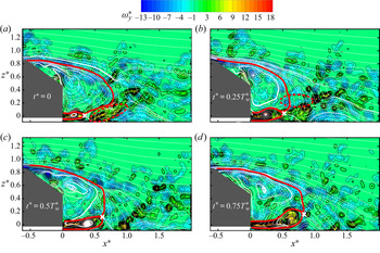
It is of interest to understand the physics behind the unsteady structures of Stw = 0.30. Figure 9 shows PIV-measured instantaneous flow structures in one typical cycle with a period  $T_w^\ast \textrm{ }({\approx} 3.3)$ of the unsteady structure generation in the symmetry plane of the wake. Following Zhang et al. (Reference Zhang, Zhou and To2015), the length l* of each bubble is defined by the maximum longitudinal length of the region where U ≤ 0. At the beginning (t* = 0) of the cycle, one organized structure characterized by the concentration of quite strong positive
 $\omega _y^\ast $ (figure 9a), as highlighted by a red broken curve, appears pinched off from the lower recirculation bubble at x* ≈ 0.4, shooting slightly upwards. At t* =
 $0.25T_w^\ast $, the upper recirculation bubble undergoes a decrease in size from l* = 0.76 at t* = 0 to l* = 0.60, accompanied by the emanation of a structure of negative
 $\omega _y^\ast $ from it (figure 9b). Then, both bubbles gradually grow in size, with l* increasing to 0.81 at t* =
 $0.75T_w^\ast $ (figure 9c,d). During the whole cycle, the upper and lower bubbles undergo a nearly periodic expansion and contraction, l* varying over [0.60, 0.81] and [0.33, 0.81], respectively. Kohri et al. (Reference Kohri, Yamanashi, Nasu, Hashizume and Katoh2014) detected a predominant frequency St ≈ 0.27 behind the Ahmed body of φ = 35° at Re = 0.73 × 10⁵, which was ascribed to the fluctuation of an upwash flow from the lower edge of the base. They advocated that the fluctuation was induced by periodic vortex shedding from the bottom end. However, the present hot-wire and PIV data suggest a different scenario. The unsteady structures of Stw = 0.30 may result from the nearly periodic expansion and contraction of both bubbles when the organized structures are either pinched off from the lower bubble or emanated from the upper bubble, with their onset at x* ≈ 0.4. More elaboration on these unsteady structures and nearly periodic variation of the bubbles will be given below.
PIV-measured instantaneous sectional streamlines and isocontours of spanwise vorticity  $\omega _y^\ast $ in one typical cycle in the symmetry plane of y* = 0 at Re = 0.62 × 10⁵. The red solid curve indicates the bubble size, determined from the sectional streamline that encloses the region of recirculation bubbles. The red broken line highlights the structure emanated from each bubble.

The spectral coherence  $Co{h_{{u_1}{u_2}}}\textrm{ }( = (Co_{{u_1}{u_2}}^2 + Q_{{u_1}{u_2}}^2)/{E_{{u_1}}}{E_{{u_2}}})$ between two fluctuations
 ${u_1}$ and
 ${u_2}$ provides a measure for the correlation between the spectral components of
 ${u_1}$ and
 ${u_2}$ (Antonia, Zhou & Matsumara Reference Antonia, Zhou and Matsumura1993), where
 $C{o_{{u_1}{u_2}}}$ and
 ${Q_{{u_1}{u_2}}}$ are the co-spectrum and quadrature spectrum of
 ${u_1}$ and
 ${u_2}$, respectively. The spectral coherence
 $Co{h_{u{B_1}u{B_3}}}$ (figure 10a) between two simultaneously measured hot-wire signals at B1 and B3 (x* = 0.43) is characterized by one predominant peak around Stw = 0.30, reaching nearly 0.35, and the corresponding spectral phase shift
 ${\varPhi _{u{B_1}u{B_3}}}\textrm{ }( = {\tan ^{ - 1}}({Q_{u{B_1}u{B_3}}}/C{o_{u{B_1}u{B_3}}}))$ is about 0.5
 ${\rm \pi}$ (figure 10b). B1 and B3 (and also C1 and C3 or D1 and D3 that follow) are as in figure 7. Similar observations are also made at x* = 0.65 (C1 and C3) and x* = 0.86 (D1 and D3), corresponding to a phase shift of 0.63
 ${\rm \pi}$ and 0.70
 ${\rm \pi}$ (not shown), respectively. Note that there is a difference in the convecting velocity between the flows at z* = 0 and 0.25, that is, the velocity of the flow from the gap between the body and the ground is higher than that in the wake around z* = 0.25 (not shown). This difference varies downstream in the near wake, accounting for the increase in
 $\varPhi$ from x* = 0.43 to 0.86. Clearly, the unsteady structures detected at B1 and B3, C1 and C3 or D1 and D3 are highly correlated. This phase shift is distinct from that of near
 ${\rm \pi}$ associated with the unsteady structures emanated from the two recirculation bubbles behind the base in the high-drag regime (Zhang et al. Reference Zhang, Zhou and To2015).
(a) Spectral coherence  $Co{h_{u{B_1}u{B_3}}}$ and (b) phase
 ${\varPhi _{u{B_1}u{B_3}}}$ between simultaneously measured hot-wire signals
 $u{B_1}$ and
 $u{B_3}$, at Re = 0.62 × 10⁵. Please refer to figure 7 for the locations of B 1 and B 3.

To gain an in-depth understanding of the unsteady structures of Stw = 0.30 and why  ${\varPhi _{u{B_1}u{B_3}}} \approx 0.5{\rm \pi} $, we performed a POD analysis of the time-resolved PIV data obtained over x* ∈ [−0.61, 1.93] and z* ∈ [−0.07, 1.34] in the symmetry plane. The POD is introduced in detail by Sirovich (Reference Sirovich1987), for example. Briefly, the spatiotemporal fluctuating velocity field u(x, t) is decomposed into an optimal set of spatial base functions
 ${\boldsymbol{\varPsi }_{\boldsymbol{n}}}(\boldsymbol{x})$ and temporal mode coefficients an(t), viz.
 \begin{equation}\boldsymbol{u}(\boldsymbol{x},\; t) = \boldsymbol{U}(\boldsymbol{x},\; t) - \bar{\boldsymbol{U}}(\boldsymbol{x}) = \sum\limits_n {{a_n}(t){\boldsymbol{\varPsi }_{\boldsymbol{n}}}(\boldsymbol{x})} ,\end{equation}
where U is the instantaneous velocity vector at the position x and n is the POD mode number. The fluctuating velocity fields from M snapshots can be arranged in a matrix  ${\boldsymbol{u}_M}$ as
 \begin{equation}{\boldsymbol{u}_M} = [\,\boldsymbol{u}({t_1})\quad \boldsymbol{u}({t_2})\quad \ldots \quad \boldsymbol{u}({t_M})\,].\end{equation}
Then, the problem can be solved by
 \begin{equation}\boldsymbol{u}_M^\textrm{T}{\boldsymbol{u}_M}{\boldsymbol{\varPhi }_n} = {\lambda _n}{\boldsymbol{\varPhi }_n},\end{equation}
where the superscript ‘T’ denotes the transpose operator,  ${\boldsymbol{\varPhi }_n}$ is the eigenvector and λn is the eigenvalue or mode energy of the nth mode, representing the contribution from the corresponding POD mode to the total turbulent kinetic energy. Solutions are sorted in order of decreasing λn so that the most energetic modes are the first few modes. Since the mean velocity field is subtracted, the Mth eigenvalue will always be zero (neglecting round-off errors). Then the normalized and spatially orthogonal base function
 ${\boldsymbol{\varPsi }_n}(\boldsymbol{x})$ can be given by
 \begin{equation}{\boldsymbol{\varPsi }_n}(\boldsymbol{x}) = \frac{{{\boldsymbol{u}_M}{\boldsymbol{\varPhi }_n}}}{{||{\boldsymbol{u}_M}{\boldsymbol{\varPhi }_n}||}},\quad n = 1,2, \ldots ,M - 1,\end{equation}
where ||…|| denotes the discrete 2-norm. The mode coefficients are determined by projecting u(x, t) onto the POD modes:
 \begin{equation}{a_n}(t) = \boldsymbol{\varPsi }_n^\textrm{T}(\boldsymbol{x})\boldsymbol{u}(\boldsymbol{x},\; t).\end{equation}
A total of M = 1000 snapshots were analysed, in which the mean velocity field, i.e. mode 0, was subtracted in data processing. Figure 11(a) shows the sensitivity of the POD relative energy contributions  ${\lambda _n}/\sum {{\lambda _n}}$ to the number of snapshots. The
 ${\lambda _n}/\sum {{\lambda _n}}$ of the first four modes (mode 0 is not included) change little when M exceeds 700. The result implies that M = 1000 is adequate if these lower POD modes are of major interest. The
 ${\lambda _n}/\sum {{\lambda _n}}$ for the first 20 POD modes (figure 11b) indicates clearly that the first four modes are the most energetic, accounting for 7.6 %, 7.0 %, 4.9 % and 3.6 % of the total turbulent kinetic energy, respectively. Therefore, our attention will be focused on those four modes in the following discussion.
(a) POD eigenvalue convergence as a function of PIV snapshot number M. (b) Relative contribution of individual POD modes for mode n ∈ [1, 20], where M = 1000. The POD analysis is conducted over x* ∈ [−0.61, 1.93] and z* ∈ [−0.07, 1.34] in the symmetry plane. Here Re = 0.62 × 10⁵.

In order to extract the periodic structures from random fluctuations, a triple decomposition is applied to the PIV data, following Hussain and Reynolds (Reference Hussain and Reynolds1970), viz.
 \begin{equation}\boldsymbol{U}(\boldsymbol{x},t) = \bar{\boldsymbol{U}}(\boldsymbol{x}) + \boldsymbol{u}(\boldsymbol{x},t) = \bar{\boldsymbol{U}}(\boldsymbol{x}) + \tilde{\boldsymbol{u}}(\boldsymbol{x},\; \phi (t)) + \boldsymbol{u^{\prime\prime}}(\boldsymbol{x},t),\end{equation}
where u is further decomposed into a nearly periodic part  $\tilde{\boldsymbol{u}}$ and a residual
 $\boldsymbol{u^{\prime\prime}}$, and ϕ is the phase angle of
 $\tilde{\boldsymbol{u}}$. The nearly periodic or coherent motion may be given in terms of
 $\bar{\boldsymbol{U}}(\boldsymbol{x}) + \tilde{\boldsymbol{u}}(\boldsymbol{x},\; \phi (t))$, obtained by a POD reconstruction. The power spectral density functions of the POD coefficients display a pronounced peak at f* ≈ 0.30 for modes 1 and 2 (figure 12a,b) but not for modes 3 and 4 (figure 12c,d) or higher modes (not shown). The observation suggests that only modes 1 and 2 are associated with the nearly periodic structures of Stw = 0.30.
Power spectra of the first four POD coefficients: (a) mode 1; (b) 2; (c) 3; and (d) 4. The POD analysis is conducted over x* ∈ [−0.61, 1.93] and z* ∈ [−0.07, 1.34] in the symmetry plane and M = 1000. Here Re = 0.62 × 10⁵.

A phase-resolved flow field may be reconstructed approximately with a low-order flow model including the mean flow (mode 0) and modes 1 and 2 (Ben Chiekh et al. Reference Ben Chiekh, Michard, Grosjean and Bera2004), viz.
 \begin{equation}{\boldsymbol{U}_{LOM}}(\boldsymbol{x},\phi ) = \bar{\boldsymbol{U}}(\boldsymbol{x}) + {a_1}(\phi ){\boldsymbol{\varPsi }_1}(\boldsymbol{x}) + {a_2}(\phi ){\boldsymbol{\varPsi }_2}(\boldsymbol{x}),\end{equation}
where  ${a_1} = \sqrt {2{\lambda _1}} \sin (\phi )$ and
 ${a_2} = \sqrt {2{\lambda _2}} \cos (\phi )$ (van Oudheusden et al. Reference van Oudheusden, Scarano, Van Hinsberg and Watt2005), viz.
 \begin{equation}\frac{{{a_1}(i)}}{{\sqrt {2{\lambda _1}} }} = {r_i}\sin ({\phi _i}),\quad \frac{{{a_2}(i)}}{{\sqrt {2{\lambda _2}} }} = {r_i}\cos ({\phi _i}).\end{equation}
The ri in (3.11) is the ‘radius’ of the normalized ellipse, viz.
 \begin{equation}r_i^2 = \frac{{{a_1}{{(i)}^2}}}{{2{\lambda _1}}} + \frac{{{a_2}{{(i)}^2}}}{{2{\lambda _2}}}.\end{equation}
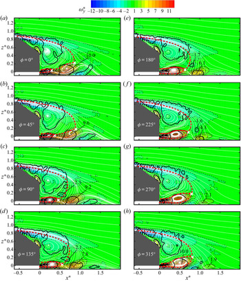
Figure 13 presents the reconstructed phase-resolved sectional streamlines viewed in a reference frame fixed on the model, superimposed with the isocontours of spanwise vorticity. The upper and lower recirculation bubbles are highlighted by red-coloured thick broken lines. The variation of the flow structure with the phase provides an insight into the formation of the nearly periodic structures of Stw = 0.30. At ϕ = 0°, one structure, marked by the contour of  $\lambda _{ci}^{2\ast } = 0.4$ with
 $\omega _{y,max}^\ast{=} 10.0$, near the hot-wire measurement point B1 (x* = 0.43, z* = 0), appears to pinch off from the lower recirculation bubble (figure 13a). The observation conforms to the emanated structure from the lower bubble, as captured in figure 9(a). As a result, the length of the lower bubble retreats markedly from its maximum l* = 0.82 at ϕ = 315° (figure 13h) to l* = 0.30 at ϕ = 0° (figure 13a). Then, the lower recirculation bubble grows gradually in size from ϕ = 0° to 315°, because of the continuous entrainment of fluid from the lower edge, until part of the bubble is pinched off again in the next cycle. Obviously, the lower bubble undergoes a nearly periodic variation in size over l* ∈ [0.30, 0.82]. This is internally consistent with the observation from the instantaneous flow structure images in figure 9. Meanwhile, the separated structure is advected downstream and its maximum vorticity decays from
 $\omega _{y,max}^\ast{=} 10.0$ at x* = 0.66 (ϕ = 0°) to
 $\omega _{y,max}^\ast{=} 1.9$ at x* = 1.16 (ϕ = 315°) (figure 13a–h). This structure is invisible beyond x* = 1.5 during the entire cycle, implying that this structure vanishes rather rapidly.
Phase-resolved reconstructed sectional streamlines (white) and spanwise vorticity within one typical cycle in the symmetry plane y* = 0. The white symbol ‘×’ denotes the saddle point. The red line indicates the bubble size, determined from the sectional streamline that encloses the region of recirculation bubbles. Black thick lines are contours of  $\lambda _{ci}^{2\ast } = 0.4$. The magnitudes of
 $\omega _{y,max}^\ast $ and
 $\omega _{y,min}^\ast $ are marked in the figure. Here Re = 0.62 × 10⁵.

The upper recirculation bubble also varies in size. At ϕ = 45°, this bubble grows to its maximum with l* = 0.90 (figure 13b). With continuously entrained fluid from the upper edge of the slanted surface, the bubble cannot maintain itself any more and bursts at ϕ = 90°, causing its size to collapse from l* = 0.90 at ϕ = 45° to l* = 0.69 at ϕ = 90° (figure 13b,c). Then, the bubble grows again, reaching l* = 0.81 at ϕ = 315° (figure 13c–h). This growth-and-burst process reflects the upper bubble variation captured in figure 9. The burst is accompanied by the separation of one swirling structure, marked by the contour of  $\lambda _{ci}^{2\ast } = 0.4$ with
 $\omega _{y,min}^\ast{=}{-} 2.3$, from the upper recirculation bubble. This structure is then advected downstream (figure 13c–f). The result is consistent with the structure emanation captured in figure 9(b). This structure decays quickly downstream, from
 $\omega _{y,min}^\ast{=}{-} 2.3$ at ϕ = 90° to
 $\omega _{y,min}^\ast{=}{-} 1.6$ at ϕ = 225°, and vanishes before x* = 1.0 at ϕ = 270° (figure 13c–g). Note that the emanation of structures from the lower and upper bubbles occurs at ϕ = 0° and 90°, respectively, which agrees approximately with
 ${\varPhi _{u{B_1}u{B_3}}} \approx 0.5{\rm \pi} $ at f* = 0.30 (figure 10).
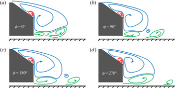
The physical process is schematically described, based on the above observations, in figure 14 for the nearly periodic variation of two recirculation bubbles and the ensuing separation of the coherent structures, responsible for Stw = 0.30. The flow separated from the lower edge of the base is entrained into the lower recirculation bubble continuously, leading to an increase in pressure within the bubble. After growing to its maximum with a certain pressure level, this bubble cannot sustain itself any more and bursts at ϕ = 0°, meanwhile ejecting one structure. The bubble contracts greatly at ϕ = 0°. This sudden contraction may correspond to a significant pressure drop in the bubble. On the other hand, the upper recirculation bubble is much bigger in size but also weaker in vorticity strength than the lower one (figure 13). This difference is markedly bigger than that in the high-drag regime (Zhang et al. Reference Zhang, Zhou and To2015). The sudden contraction and pressure drop of the lower bubble may naturally disturb the upper bubble and induce its bursting at ϕ = 90°, accompanied by the emanation of a coherent structure. This may explain the phase shift of about 0.5 ${\rm \pi}$ at f* = 0.30 (figure 10b). This phase shift may imply a relatively strong interaction between the structures emanated from the two bubbles and hence a short lifespan, vanishing by x* = 1.29 (figure 7). In contrast, their counterparts in the high-drag regime are in antiphase and persist till x* = 1.40 (Zhang et al. Reference Zhang, Zhou and To2015). After bursting, the bubble starts its growth in size and pressure of the next cycle, and the separated structures are advected downstream, though decaying rapidly.
Schematic of the physical process for the nearly periodic motion of two recirculation bubbles and separated flow structures that result.

The second moments of the fluctuating velocities in the wake may have an important impact on the surface pressure on the rear part of a bluff body (e.g. Balachandar, Mittal & Najjar Reference Balachandar, Mittal and Najjar1997; Barros et al. Reference Barros, Borée, Noack, Spohn and Ruiz2016b). Following Grandemange et al. (Reference Grandemange, Gohlke and Cadot2013), we may write the streamwise mean momentum balance of the recirculation region, where the viscous force is neglected, behind a low-drag Ahmed body as
 \begin{align}\langle {C_p}\rangle {H^\ast }{W^\ast } & = \int_{\partial B} {{C_{pw}}(\boldsymbol{n}\boldsymbol{\cdot }{\boldsymbol{i}_x})\,\textrm{d}{B^\ast }} + 2\int_{\partial B} {\overline {{u^\ast }{u^\ast }} (\boldsymbol{n}\boldsymbol{\cdot }{\boldsymbol{i}_x})\,\textrm{d}{B^\ast }} + 2\int_{\partial B} {\overline {{u^\ast }{v^\ast }} (\boldsymbol{n}\boldsymbol{\cdot }{\boldsymbol{i}_y})\,\textrm{d}{B^\ast }} \nonumber\\ & \quad + 2\int_{\partial B} {\overline {{u^\ast }{w^\ast }} (\boldsymbol{n}\boldsymbol{\cdot }{\boldsymbol{i}_z})\,\textrm{d}{B^\ast }},\end{align}
where ix, iy and iz are the unit vectors of the coordinate system, n is the local unit vector normal to the differential element dB* of the three-dimensional recirculation boundary ∂B,  $\langle {C_p}\rangle $ is the spatially averaged Cp on the rear end, and Cpw is the local time-averaged pressure coefficient in the wake. Equation (3.13) shows a close connection between the Reynolds stresses along the recirculation region boundary and the pressure drag. Given the symmetry conditions in the plane of y* = 0,
 $\boldsymbol{n}\boldsymbol{\cdot }{\boldsymbol{i}_y}$ is zero so that the term
 $\overline {{u^\ast }{v^\ast }} (\boldsymbol{n}\boldsymbol{\cdot }{\boldsymbol{i}_y})$ vanishes in the mean recirculation region, as Barros et al. (Reference Barros, Borée, Noack, Spohn and Ruiz2016b) did for a square-back Ahmed body. Then, the sum of the integrations on the right-hand side of (3.13) may be reduced to a two-dimensional form (Balachandar et al. Reference Balachandar, Mittal and Najjar1997), namely,
 \begin{equation}C = \int_{\partial b} {{C_{pw}}(\boldsymbol{n}\boldsymbol{\cdot }{\boldsymbol{i}_x})\,\textrm{d}{b^\ast }} + 2\int_{\partial b} {\overline {{u^\ast }{u^\ast }} (\boldsymbol{n}\boldsymbol{\cdot }{\boldsymbol{i}_x})\,\textrm{d}{b^\ast }} + 2\int_{\partial b} {\overline {{u^\ast }{w^\ast }} (\boldsymbol{n}\boldsymbol{\cdot }{\boldsymbol{i}_z})\,\textrm{d}{b^\ast }} ,\end{equation}
where db* is the differential element of the in-plane recirculation boundary ∂b in the plane of y* = 0.
Figure 15 presents the time-averaged normal stresses  $\overline {{u^\ast }{u^\ast }} $ and
 $\overline {{w^\ast }{w^\ast }} $, and shear stress
 $\overline {{u^\ast }{w^\ast }} $ in two x–z planes of y* = 0 and 0.36, where the recirculation boundary enclosing the upper and lower recirculation bubbles is highlighted by a red-coloured broken curve as determined from the time-averaged sectional streamlines (figure 2). Several observations may be made. Firstly, the
 $\overline {{u^\ast }{u^\ast }} $ contours display two concentrations (figure 15a,b). One occurs behind the rear window, which is apparently associated with the shear layer separated from the upper edge of the slanted surface. The other takes place downstream of the lower edge of the base. In the symmetry plane, this concentration spatially coincides with the structure of Stw = 0.30 detected behind the base (figure 7) and is connected to the nearly periodic motions of the upper and lower bubbles and hence the structures emanated from the bubbles. Secondly, the
 $\overline {{w^\ast }{w^\ast }} $ contours display one highly concentrated region behind the vertical base (figure 15c,d). The rollup of the gap flow and the downwash flow from the rear window appear to clash with each other near (x*, z*) ≈ (0.78, 0.08) in the symmetry plane of y* = 0 and (0.75, 0.42) in the off-symmetry plane of y* = 0.36 based on the PIV-measured streamlines (figure 2a,c), which may account for this concentration. Thirdly, two opposite-signed concentrations are evident in the
 $\overline {{u^\ast }{w^\ast }} $ contours in both x–z planes (figure 15e,f). The upper is negative while the lower is positive, which are linked to the upper and lower recirculation bubbles, respectively.
Isocontours of PIV-measured time-averaged in-plane Reynolds stresses in the x–z planes of y* = 0 and y* = 0.36. Thick broken red curves indicate the recirculation boundary determined from sectional streamlines in figure 2. The black symbol ‘×’ denotes the dividing point in the boundary where  $\overline {{u^\ast }{w^\ast }} = 0$. Here Re = 0.62 × 10⁵.

In order to evaluate the effect of the  $\overline {{u^\ast }{u^\ast }} $ and
 $\overline {{u^\ast }{w^\ast }} $ concentrations of each bubble on
 $\langle {C_p}\rangle $, ∂b in the symmetry plane is divided into two parts (∂bu and ∂bl) by the dividing point where
 $\overline {{u^\ast }{w^\ast }} $ equals zero, as marked by the black symbol ‘×’ at (x*, z*) ≈ (0.78, 0.2) (figure 15a,g). The subscripts u and l denote the upper and lower bubbles, respectively. Then, the sum of the integrations of
 $\overline {{u^\ast }{u^\ast }} $ and
 $\overline {{u^\ast }{w^\ast }} $ along ∂bu and ∂bl can be written as
 \begin{equation}C_i^R = \int_{\partial {b_i}} {\overline {{u^\ast }{u^\ast }} (\boldsymbol{n}\boldsymbol{\cdot }{\boldsymbol{i}_x})\,\textrm{d}{b^\ast }} + \int_{\partial {b_i}} {\overline {{u^\ast }{w^\ast }} (\boldsymbol{n}\boldsymbol{\cdot }{\boldsymbol{i}_z})\,\textrm{d}{b^\ast }} ,\quad i \in \{ u\;\textrm{or}\;l\} .\end{equation}
The  $C_u^R$ and
 $C_l^R$ are calculated to be approximately −0.005 and −0.007 in the symmetry plane, which contribute negatively to
 $\langle {C_p}\rangle $. As will be shown in § 4, the structures of Stw = 0.30 show up in the region of x* ∈ [0.43, 0.86], y* ∈ [−0.29, 0.29] and z* ∈ [−0.04, 0.32]. The Reynolds stress distribution in an off-symmetry plane of y* = 0.14 also displays the concentrations of
 ${\overline {{u^\ast }{u^\ast }} _{max}} = 0.052$ at (x*, z*) = (0.69, 0.02) and
 ${\overline {{u^\ast }{w^\ast }} _{max}} = 0.034$ at (x*, z*) = (0.81, 0.05) (not shown), due to the presence of this unsteady structure. It may be inferred from the relationship between the Reynolds stresses and
 $\langle {C_p}\rangle $ that this unsteady structure may have a considerable impact on the base and rear window pressures in the off-symmetry planes, as in the symmetry plane. The structures emanated alternately from the upper and lower bubbles may produce a substantial turbulent kinetic energy k*
 $=0.5(\overline {{u^\ast }{u^\ast }} + \overline {{w^\ast }{w^\ast }} )$, as supported by the
 $\overline {{u^\ast }{u^\ast }} $ and
 $\overline {{w^\ast }{w^\ast }} $ concentrations associated with these structures (figure 15). If we consider a vehicle cruising in ambient still fluid, the energy loss due to the turbulent kinetic energy consumes part of the work done on the fluid, and hence increases the vehicle pressure drag. That is, the emanated structures contribute to a rise in the drag.
3.4. Roof, sidewall and gap vortices
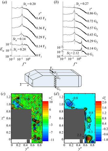
The Eu measured above the roof at x* = −1.27 and z* = 0.94 displays two major peaks (figure 16a) at f* = Str = 0.20 for F1 (y* = 0) and from F3 to F5 (y* ∈ [0.29, 0.43]) and at f* = Sta = 0.14 for F2 (y* = 0.14). A streamwise vortex with negative vorticity is captured instantaneously above the roof around y* = 0.14 (figure 16c), which is responsible for the time-averaged swirling structure (marked by  $\bar{\lambda }_{ci}^{2\ast } = 0.002$) with
 $\bar{\omega }_{x,min}^\ast{=}{-} 0.8$ at y* = 0.14 and z* = 0.98 (figure 16d). This vortex is spatially coincident with the detected Sta = 0.14. The Str = 0.20 is associated with the hairpin vortices emanated from the separation bubble near the leading edge of the roof, and Sta = 0.14 is linked to the oscillation of one pair of longitudinal counter-rotating vortices behind the bubble, whose origins are the two foci at each end of the flow separation line (Zhang et al. Reference Zhang, Zhou and To2015). When viewed in the y–z plane, the vortex at y* = 0.14 is clockwise and the other at y* = −0.14 must be anticlockwise. Therefore, the tangential velocity at the inner side of each longitudinal vortex about the symmetry plane is upwards. Thus, at y* ∈ [−0.14, 0.14], the longitudinal vortices may act to push up the hairpin vortices to the outer flow with a higher convection velocity to get diffused, which may be responsible for the relatively weak peak of Str = 0.20 in Eu at F1 (y* = 0) (figure 16a).
Power spectral density function Eu of the hot-wire signal measured along (a) F1–F5 (x* = −1.27, z* = 0.94) above the roof, and (b) G1–G7 (x* = −1.27, y* = 0.63) near the sidewall, respectively. PIV-measured (c) typical instantaneous and (d) time-averaged streamwise vorticity contours in the y–z plane of x* = −1.27. Thick black closed contours correspond to the swirling strength  $\bar{\lambda }_{ci}^{2\ast } = 0.002$ of the time-averaged flow. The magnitudes of
 $\bar{\omega }_{x,max}^\ast $ and
 $\bar{\omega }_{x,min}^\ast $ are marked in the figure. Here Re = 0.62 × 10⁵.

The Eu measured over the sidewall at x* = −1.27 and y* = 0.63 (figure 16b) shows one pronounced peak at f* = Sts = 0.27 over z* ∈ [0.14, 0.72] (G2–G6). As above the roof, Sts is associated with the side vortices emanated from the separation bubble near the leading edge of the sidewall. At G4 (z* = 0.43) near the mid-height of the sidewall, this peak is less pronounced, similarly to the case at F1 above the roof in the symmetry plane (figure 16a), with the same flow physics involved, as is evident from one pair of counter-rotating longitudinal vortices over the sidewall about the mid-height of the body (figure 16c,d). Another predominant frequency of f* = Stl = 2.12 is detected at G1–G2 near the lower edge of the sidewall (figure 16b), which is ascribed to the vortices generated by the upstream struts located at x* = −2.52 and y* = ±0.49 (Zhang et al. Reference Zhang, Zhou and To2015).
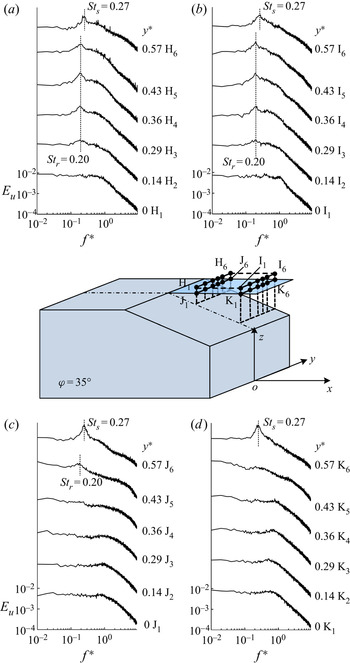
In view of the strong three-dimensionality of the flow, the hot-wire measurements were performed at various spanwise locations over the slanted surface, as shown in figure 17. A peak at Str = 0.20 is discernible at H3–H5 (x* = −0.36, y* ∈ [0.29, 0.43], z* = 0.91) near the upper edge of the rear window and at I3–I5 (x* = −0.09, y* ∈ [0.29, 0.43], z* = 0.91) further downstream (figure 17a,b). However, this peak becomes less pronounced at H2 and I2 (y* = 0.14) near the symmetry plane, and even vanishes at H1 and I1 (y* = 0), which may be linked to the interaction between these structures with the longitudinal vortices above the roof near the symmetry plane (figure 17a,c,d). In addition, Str is not detectable in Eu measured at J1–J4 and K1–K5 at the height of the roof (z* = 0.86) (figure 17c,d) and also at lower positions (not shown), indicating that these vortices travel above the upper recirculation bubble.
Power spectral density function Eu of the hot-wire signal measured along (a) H1–H6 (x* = −0.36, z* = 0.91), (b) I1–I6 (x* = −0.09, z* = 0.91), (c) J1–J6 (x* = −0.36, z* = 0.86) and (d) K1–K6 (x* = −0.09, z* = 0.86), respectively, over the slant. Here Re = 0.62 × 10⁵.

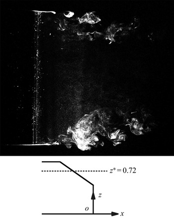
A peak occurs at Sts = 0.27 in Eu measured at H6, I6, J6 and K6 near the side edge of the rear window (y* = 0.57) (figure 17), where the C-pillar vortex takes place (figure 5). A typical photograph captured in the x–y plane of z* = 0.72 over the rear window (figure 18) exhibits nearly periodic structures right above the side edges of the rear window. Obviously, this image should cut through the C-pillar vortices. Then, these nearly periodic structures reconfirm Zhang et al.'s (Reference Zhang, Liu, Zhou, To and Tu2018) assertion that the side vortices may wrap around and get tangled with the C-pillar vortex.
Typical photograph of the flow structure in the x–y plane of z* = 0.72 at Re = 0.22 × 10⁵. Flow is from left to right.

In order to detect possible nearly periodic structures formed in the gap between the ground and the underside of the Ahmed body, hot-wire measurements were conducted along L1–L7 (x* = 0.09, z* = 0), downstream of the lower edge of the base (figure 19). Two prominent frequencies occur at L3–L7 (y* ∈ [0.36, 0.79]) in Eu. One is f* = Stg = 1.77 at L3–L5 over y* ∈ [0.36, 0.65], spatially corresponding to the gap vortex captured by Wang et al. (Reference Wang, Zhou, Pin and Chan2013). Another is f* = Stl = 2.12 at L6–L7 over y* ∈ [0.72, 0.79], outside the lower corner of the base, spatially coinciding with the lower vortex, which originates from the vortices detected at G1–G2 at the lower edge of the sidewall (figure 16b).
Power spectral density function Eu of the hot-wire signal measured along J1–J7 (x* = 0.09, z* = 0) in the wake, at Re = 0.62 × 10⁵.

4. Spatial extent of unsteady structures
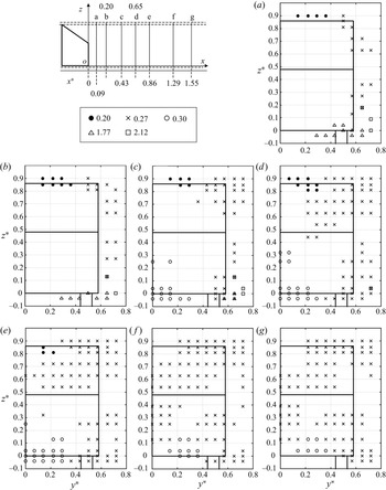
The locations and extents where the five distinct vortices and their frequencies, i.e. Str, Sts, Stw, Stg and Stl, were detected in the y–z planes vary for different downstream stations due to the three-dimensionality of the wake. Figure 20 presents their spatial distributions in the y–z planes of x* ∈ [0.09, 1.55]. The vortices of Sti (i = r, s, w, g or l) are considered to occur when the ratio of the Hertz-averaged energy in Eu over  $St \in [S{t_i} - 0.01;\,S{t_i} + 0.01]$ to that over
 $St \in [S{t_i} - 0.15;\,S{t_i} + 0.15]$ exceeds 1.3, at which a pronounced peak can be seen at Sti in Eu (Grandemange et al. Reference Grandemange, Gohlke and Cadot2013).
Locations where the predominant vortex frequencies are detected in the y–z planes at (a) x* = 0.09, (b) x* = 0.20, (c) x* = 0.43, (d) x* = 0.65, (e) x* = 0.86, (f) x* = 1.29 and (g) x* = 1.55. Here Re = 0.62 × 10⁵.

The hairpin vortices of Str = 0.20 from the roof are detectable at z* = 0.9 over y* ∈ [0.14, 0.36] in the plane of x* = 0.09 (figure 20a). Further downstream at x* = 0.20, 0.43 and 0.65 (figure 20b–d), these structures expand slightly downwards to z* = 0.81. The extent where Str = 0.20 is detected shrinks in the region of 0.14 ≤ y* ≤ 0.22 and 0.81 ≤ z* ≤ 0.86 in the plane of x* = 0.86 (figure 20e), and vanishes completely beyond the plane of x* = 1.29 (figure 20f,g), that is, the hairpin vortices disappear.
In the plane of x* = 0.09 (figure 20a), the side vortices of Sts = 0.27 are discernible in two regions behind the side edge of the rear window and that of the base. However, this frequency cannot be captured for z* ∈ [0.4, 0.6] about the sidewall, due to the interaction of these vortices with the longitudinal vortices near the mid-height of the sidewall (figure 16b–d). Beyond x* = 0.43 (figure 20c), the upper detections of Sts = 0.27 expand both downwards and inwards, covering most of the region above the upper edge of the vertical base by x* = 0.65 (figure 20d); by x* = 1.29 (figure 20f), the structures spread over the central region and reach z* = 0.13 near the lower edge of the base. The other region of Sts = 0.27 near the lower sidewall reaches the lower edge of the vertical base at x* = 0.43 (figure 20c) and grows considerably around the lower corner of the base from x* = 0.86 (figure 20e–g). As the vortices may interact with and wrap up around the longitudinal trailing vortices, Sts = 0.27 is identifiable over x* ∈ [1.29, 1.55] in the wake (figure 20f,g). This is quite different from the high-drag regime where only the unsteady structures of St = 0.44 persist downstream of the recirculation bubbles over x* ∈ [1.4, 2.2] (Zhang et al. Reference Zhang, Zhou and To2015). In the high-drag regime, the vibrant C-pillar vortices interact with the side vortices and tend to accelerate the breakup of the latter; while in the low-drag regime, the weak ones would have a very small effect on the latter. Thus, the side vortices may persist further downstream.
The structures of Stw = 0.30 emerge at x* = 0.43 around the mid-height and lower edge of the base (figure 20c). The upper detections (z* > 0.20) are associated with the structures from the upper recirculation bubble. The region enclosing the detections grows from x* = 0.43 to 0.65 (figure 20c,d) but contracts appreciably beyond x* = 0.86 (figure 20e). The structures vanish completely by x* = 1.29 (figure 20f) where the unsteady structures of Sts = 0.27 persist. The lower detections (z* < 0.20) of Stw = 0.30 associated with the structures from the lower bubble expand transversely from x* = 0.43 to 0.86 (figure 20c–e) and then spread upwards at x* = 0.86 (figure 20e). The region enclosing these detections recedes, from x* = 0.86 to 1.55 (figure 20e–g), away from the centreline. While advected downstream, the structures from the lower bubble may interact with the developing longitudinal trailing vortices and be drawn transversely away from the plane of symmetry. Apparently, the structures originated from the lower bubble persist longer than those from the upper bubble, which is internally consistent with the observation from figure 13. Note that Stw = 0.30 fails to be captured in the off-symmetry region of y* > 0.3 for x* < 1.29 (figure 20c–e). That is, the corresponding unsteady structures occur largely only around the plane of y* = 0.
At x* = 0.09 (figure 20a), Stg = 1.77 associated with the gap vortices is detected around the cylindrical support at y* ∈ [0.29, 0.65] and z* ∈ [−0.04, 0.04], while Stl = 2.12 is captured outside the lower corner at y* = 0.72 and z* ∈ [0, 0.09]. The two frequencies completely disappear beyond x* = 0.65.
5. Reynolds-number effect
The information on St is crucially important for developing an effective active drag reduction technique (e.g. Brunn & Nitsche Reference Brunn and Nitsche2006; Joseph et al. Reference Joseph, Amandolese and Aider2012; Barros et al. Reference Barros, Borée, Noack, Spohn and Ruiz2016b; Tounsi et al. Reference Tounsi, Mestiri, Keirsbulck, Oualli, Hanchi and Aloui2016). However, the relationship between Re and St in the low-drag regime has not been well documented in the literature. In this section, the possible dependences of the five predominant unsteady structures on Re are investigated based on hot-wire measurements over Re ∈ [0.3, 2.7] × 105. Figure 21 presents the variations of Str, Sts, Stw, Stg and Stl with Re, along with the data available in the literature for the same Ahmed body of φ = 35° for comparison. A number of observations can be made.
Dependence of the Strouhal numbers on Re.

Firstly, Stw varies little for the Re range examined, indicating a relatively weak Re effect. Kohri et al. (Reference Kohri, Yamanashi, Nasu, Hashizume and Katoh2014) detected St ≈ 0.27 at Re = 0.73 × 10⁵ in the symmetry plane downstream of the lower edge of the base for the same Ahmed body (φ = 35°), which is reasonably close to the present Stw (= 0.30). The slight deviation is probably due to the differences in facilities, measurement techniques, etc., between the two experiments. Note that Stw at φ = 25° increases nonlinearly from 0.44 to 0.54 from Re = 0.45 × 10⁵ to 2.4 × 10⁵ (Zhang et al. Reference Zhang, Zhou and To2015), which is more appreciable than the present low-drag regime. Vino et al. (Reference Vino, Watkins, Mousley, Watmuff and Prasad2005) also observed in the high-drag regime (φ = 30°) that this frequency increased from 0.36 to 0.39 over Re ∈ [4.40, 7.68] × 105. The comparison suggests that the Re effect on Stw is different between the low- and high-drag regimes. In their study on the wake of an Ahmed body (φ = 25°), Joseph et al. (Reference Joseph, Amandolese and Aider2012) observed a longitudinal shrinkage in the separation region over the rear window as Re was increased from 4.5 × 10⁵ to 9.0 × 10⁵. The shrunk separation region may influence significantly the downstream reattaching flow over the rear window. Thacker et al. (Reference Thacker, Aubrun, Leroy and Devinant2012) found from their PIV data obtained in the wake of the Ahmed body (φ = 25°) that the flow separation over the slanted surface was suppressed by rounding the upper edge of the rear window, which led to a rise in the velocity magnitude of the reattaching flow before separating again at the upper edge of the base. It is therefore inferred that, in the high-drag regime, the reduced separation region over the slanted surface with increasing Re may increase the momentum of flow separated from the upper edge of the base before being entrained into the upper recirculation bubble, and hence affect Stw. In contrast, in the low-drag regime, the two bubbles are little affected in size by Re due to their fixed separation points. As such, Stw remains nearly unchanged at 0.3 in the Re range from 0.3 × 10⁵ to 2.7 × 10⁵ (figure 21).
The measured Str and Sts increase linearly for higher Re, fitting reasonably well to Str = 0.143 + 0.070Re/105 and Sts = 0.171 + 0.126Re/105, respectively. Zhang et al. (Reference Zhang, Zhou and To2015) suggested that the frequency fj ( j = r or s) of the hairpin vortices is dictated by  ${f_j}\sim {U_\infty }/{x_{Rj}}$ (where xRj is the length of the bubble near the leading edge). Then, Stj can be rewritten as
 $S{t_j}\sim \sqrt A /{x_{Rj}} = 1/x_{Rj}^\ast $. The rise in Str and Sts with increasing Re may be attributed to a contraction in
 $x_{Rj}^\ast $, and the different slopes in Str and Sts versus Re are ascribed to a difference in the contraction rate between
 $x_{Rr}^\ast $ and
 $x_{Rs}^\ast $. The Stg and Stl values vary little in the Re range examined. Their values, about 1.84 and 2.15, respectively, are very close to their counterparts Stg ≈ 1.77 and Stl ≈ 2.12 in the high-drag regime (Zhang et al. Reference Zhang, Zhou and To2015). The corresponding coherent structures are generated by the downstream and upstream cylindrical struts, respectively. The Strouhal number in a circular cylinder wake remains nearly constant at Std ≈ 0.21 over a quite large range of
 $R{e_d} \in [3.0 \times {10^2},1.0 \times {10^5}]$, where Std and Red are based on the cylinder diameter (Schlichting & Gersten Reference Schlichting and Gersten2000), thus accounting for the independence of Stg and Stl on Re. On the other hand, Stg is smaller than Stl by about 14 %, as the gap flow is decelerated downstream by the thickening boundary layers over the floor and the model underside.
6. A conceptual model of the flow structure
A conceptual model is proposed for the flow structure around an Ahmed model in the low-drag regime (figure 22) based on the present data and those in the literature. This model has incorporated three original findings in this work. One is the formation of the corner vortex and its dynamical role. The second is the wake vortices of Stw ≈ 0.30 and their formation process. The third is the relationship between the relatively weak C-pillar vortices and the upper recirculation bubble, along with the evolution and formation of the trailing vortices. This model provides a full picture of the flow structures in the low-drag regime, which covers steady and unsteady structures above the roof, over the sidewall and the rear window, and behind the base, all based on the data in the literature as well as the present data.
A conceptual model of the flow structure around the Ahmed model in the low-drag regime (φ = 35°).

The flow reattaches soon after its separation near the leading edge of the roof, forming a separation bubble that pulsates periodically (Minguez et al. Reference Minguez, Pasquetti and Serre2008). One pair of predominantly longitudinal counter-rotating vortices takes place behind the bubble (figure 16c,d), which is originated from two foci at the ends of the separation line (Spohn & Gilliéron Reference Spohn and Gilliéron2002). Owing to the bubble pulsation, the cores of these longitudinal vortices oscillate at Sta ≈ 0.14 (figure 16a). Three-dimensional hairpin vortices are emanated from the bubble and are advected downstream along the roof (Krajnović & Davidson Reference Krajnović and Davidson2005b; Franck et al. Reference Franck, Nigro, Storti and D'elia2009), which are responsible for Str = 0.20 (figure 16a). The longitudinal vortex pair interacts with the hairpin vortices, accelerating the breakup of the latter near the symmetry plane (figure 16a). By the same token, the side vortices of Sts = 0.27 are emanated behind the separation bubble formed near the leading edge of each sidewall (figure 16b). Another pair of predominantly longitudinal counter-rotating vortices are generated from the two ends of this separation bubble (figure 16c,d). Apparently, the flow over the side surface cannot be symmetric because of the presence of the ground. Near the ground, flow rolls up about the lower edge of the sidewall under the pressure difference between the flows inside and outside of the gap (Wang et al. Reference Wang, Zhou, Pin and Chan2013), forming the lower vortex (figure 16c,d). This structure decays gradually downstream behind the base (figure 6). Vortices are generated by the upstream struts and wrapped up by the lower vortex, responsible for the detected Stl = 2.12 near the bottom of the sidewall (figure 16b).
The flow coming off the roof separates at the upper sharp edge of the rear window and fails to reattach on the slanted surface, rolling up behind the base to form a big separation bubble, covering both rear window and most of the upper part of the base (figure 2). The C-pillar vortices are greatly weakened, as compared with the high-drag regime, due to a reduced pressure difference between the flow over the rear window and that coming off the sidewall. Their cores are deflected further away from the slanted surface as compared with the high-drag case at φ = 25° (figure 5). The weak C-pillar vortices make the wake much less three-dimensional than in the high-drag regime case (e.g. Ahmed et al. Reference Ahmed, Ramm and Faltin1984; Lienhart & Becker Reference Lienhart and Becker2003).
Within the big upper recirculation bubble, an upwash flow near the upper base separates from the corner between the rear window and the vertical base and rolls up (figures 2a and 4b) under the pressure difference between the base flow and that over the rear window (figure 4a) as well as the induction of the negative circulation within the bubble. Thus a corner vortex is formed near the lower edge of the rear window, extending transversely almost over the entire width of the body (figure 3). The upper recirculation bubble results in a considerable rise in pressure on the slanted surface, compared with its counterpart in the high-drag regime (Ahmed et al. Reference Ahmed, Ramm and Faltin1984; Lienhart & Becker Reference Lienhart and Becker2003), at a small expense to bring down slightly the pressure on the upper base. On the other hand, there is a small pressure drop near the lower end of the window where the corner vortex occurs (figure 4). Zhang et al. (Reference Zhang, Liu, Zhou, To and Tu2018) deployed a combination of steady actuations along the upper and two side edges of the rear window, and along the lower edge of the base to manipulate the flow around an Ahmed body (φ = 25°). This manipulation acted to join the flow separation bubble over the slanted surface and the upper recirculation bubble behind the base. The resulting flow topology was quite similar to that in the low-drag regime (figure 2), though without the presence of the corner vortex. As a result, drag reduction reached 26 % and the corresponding drag coefficient was down to 0.267, even lower than its counterpart (0.32) by 17 % in the low-drag regime at the same Re. It is therefore plausible that the corner vortex may act as a partition to separate the high-pressure flow in the base region from the relatively low-pressure flow over the entire slanted surface, playing a significant role in the wake dynamics.
The nearly periodic structures pinched off from the lower recirculation bubble and those emanated from the upper bubble are characterized by a phase shift of about 0.5 ${\rm \pi}$ (figures 9, 10 and 13), not
 ${\rm \pi}$ as in the high-drag regime case (Zhang et al. Reference Zhang, Zhou and To2015). These structures are characterized by a predominant frequency of Stw ≈ 0.30 for
 $Re \in [0.3,2.7] \times {10^5}$ (figures 7, 20 and 21). The structures originated from the lower bubble persist longer than those from the upper bubble (figures 13 and 20).
The upper recirculation bubble extends transversely about the symmetry plane, but tilts downstream near each lateral side of the body under the effect of the streamwise flow from the sidewall (figure 2), forming a horseshoe vortex (figures 3 and 6). The legs of this horseshoe vortex develop inwards and downwards downstream. So do the pair of C-pillar vortices (figure 6a–c). Further downstream, however, the relatively weak C-pillar vortices merge into the horseshoe vortex legs and vanish quickly. It is the downstream tilting legs of the upper recirculation bubble that form the trailing vortices (figure 6).
The structures formed above the roof and the side surface have a great impact on the instability of the wake. Firstly, the hairpin vortices from the roof flow over the upper recirculation bubble, which are responsible for the measured Str = 0.20 in the shear layer separated from the upper edge of the rear window (figures 17 and 20). Secondly, the side vortices may be wrapped up by the C-pillar vortices (figure 18), accounting for the detected Sts = 0.27 above the side edge of the rear window (figure 17). This frequency also shows up downstream of the base, even beyond x* = 1.55, coinciding with the trailing vortices.
The gap vortices (Stg = 1.77) and the vortices from the upstream struts (Stl = 2.12) are detected near the lower edge of the vertical base (figure 19). These vortices decay rather quickly when convected downstream (figure 20).
Some remarks are due on the major differences between the low- and high-drag regimes. Firstly, the two recirculation bubbles occur behind the base in the high-drag regime. Flow separates from the upper edge of the rear window and then reattaches downstream, forming a separation bubble over the rear window. It is flow separation from the upper and lower edges of the base that forms the two recirculation bubbles. In the low-drag regime, however, the formation of the upper recirculation bubble is totally different. A big upper recirculation bubble is formed due to flow separating from the upper edge of the window and shooting over the base. Within this bubble, the relatively high-pressure fluid behind the base is recirculated towards the window, raising its pressure, contributing to the low drag.
Secondly, the formation of the two trailing vortices is different. The C-pillar vortices in the high-drag regime are very strong, snatching the lateral part of the upper recirculation bubble behind the base and forming the trailing vortices (Ahmed et al. Reference Ahmed, Ramm and Faltin1984; Venning et al. Reference Venning, Lo Jacono, Burton, Thompson and Sheridan2017). In contrast, the C-pillar vortices are very weak in the low-drag regime and vanish quickly. The trailing vortices originate from the downstream tilting legs of the upper recirculation bubble (figure 6) and are much weaker in strength than their counterparts in the high-drag regime. This weak strength implies a small magnitude of the dynamic pressure, which is the source of the ‘vortex drag’ (Hucho & Sovran Reference Hucho and Sovran1993), and hence accounts, along with the relatively high pressure on the rear window due to the big recirculation bubble, for the small drag in the low-drag regime.
Finally, there is a difference in the wake vortices; Stw remains nearly constant at 0.3 for Re ∈ [0.45, 2.4] × 105 in the low-drag regime but rises from 0.44 to 0.54 over the same Re range in the high-drag regime (Zhang et al. Reference Zhang, Zhou and To2015). The wake vortices are emanated alternately from the two recirculation bubbles, which grow and burst. The upper recirculation bubble in the low-drag regime originates from flow separation from a fixed point, the upper edge of the rear window. The thus formed vortices are less Re-dependent. In the high-drag regime, the separation region over the slanted surface contracts at the higher Re, which is accompanied by an increase in the momentum of the downstream reattaching flow. The higher momentum of the flow separated from the upper edge of the base accounts for a rise in Stw.
7. Conclusions
An experimental investigation has been conducted on the flow structure around a low-drag Ahmed body with a slant angle of φ = 35° at Re ∈ [0.3, 2.7] × 105. Extensive hot-wire measurements have been conducted at more than 1500 points around the body. Flow visualization, PIV and pressure measurements have also been performed. The data have been carefully analysed. The following conclusions can be drawn out of this investigation.
A total of five distinct predominant frequencies have been detected in the wake, two over the rear window and three behind the vertical base. Over the rear window,  $S{t_r} \in [0.17,0.35]$ is detected in the region off the symmetry plane and higher than the roof. The corresponding unsteady structures originate from the hairpin vortices emanated from the separation bubble near the leading edge of the roof. Another unsteady structure of
 $S{t_s} \in [0.21,0.35]$ is detected near the sidewall of the model, referred to as the side vortex emanated from the bubble near the leading edge of the sidewall, which wraps around the weak C-pillar vortex. Behind the vertical base, the unsteady structures of Stg ≈ 1.77 and Stl ≈ 2.12 captured near the lower edge of the vertical base are attributed to vortices generated by the downstream and upstream cylindrical struts, respectively. These four unsteady structures are also captured in the high-drag regime (Zhang et al. Reference Zhang, Zhou and To2015). Another distinct predominant frequency of Stw ≈ 0.30 is captured in the central region behind the vertical base, which is attributed to the nearly periodic structures emanated from the upper recirculation bubble and those pinched off from the lower bubble. This structure is different from that found in the high-drag regime.
Firstly, the nearly periodic structures are emanated at a significantly higher frequency, Stw = 0.44 for Re = 0.62 × 10⁵, from two recirculation bubbles in the high-drag regime (Zhang et al. Reference Zhang, Zhou and To2015). Secondly, the emanated structures from the two bubbles are characterized by a phase shift of about 0.5 ${\rm \pi}$ in the low-drag regime, while those in the high-drag regime are in antiphase (Zhang et al. Reference Zhang, Zhou and To2015). This difference is connected to the marked disparity in the size and strength of the upper recirculation bubble between the two regimes. This non-antiphase behaviour between the structures emanated from the two bubbles accounts for the short lifespan of these structures in the low-drag regime. Finally, Stw increases with increasing φ in the high-drag regime but remains constant in the low-drag regime. It is found that Stw scales with the vertical distance S between the separation points of the two recirculation bubbles. As the effective separation angle θ of the separated shear layer that forms the upper bubble may affect Stw, the characteristic length may be corrected by αS (α = (90° − θ)/90°), which reflects physically the bubble size. A small S or a large θ corresponds to a small bubble size and subsequently a large Stw. As a result, all Stw data collapse to
 $St_w^ +\approx 0.20$, irrespective of the value of φ or the flow regimes.
A small corner vortex is formed near the lower edge of the rear window. The pressure on the base is higher than that on the rear window. This pressure disparity, along with the induction of the negative circulation of the big bubble, drives an upwash and backward flow, forming this corner vortex. This structure plays a significant role in the wake dynamics, acting to separate the high-pressure flow behind the base from the low-pressure flow over the rear window.
The Reynolds-number effects on these unsteady structures have been investigated. The effect of Re on Stw ≈ 0.30 is negligibly small over the Re range examined (Re ∈ [0.3, 2.7] × 105). The dependences of Str, Sts, Stl and Stg on Re are similar to their counterparts in the high-drag regime because the origins of the corresponding unsteady structures are the same for the two regimes.
Based on the present data and those reported in the literature, a conceptual model is proposed for the flow structure around an Ahmed body in the low-drag regime, which provides a rather comprehensive picture for the complex flow. The present findings are incorporated into this model, including the wake vortices of Stw ≈ 0.30 and their formation process, the corner vortex and its dynamical role, the interaction between the C-pillar vortex and the upper recirculation bubble leg, and the formation and development of the longitudinal trailing vortex. Previously reported coherent structures, such as the hairpin vortices, side vortices, gap vortices and lower vortices, are also included. The dimensionless frequencies are identified for the unsteady structures.
Funding
Y.Z. wishes to acknowledge support given to him from NSFC through grants 11632006 and 91952204 and from the Research Grants Council of Shenzhen Government through grant JCYJ20190806143611025. B.F.Z. is grateful for the financial support from NSFC through grant 11902102. Z.Y.C. acknowledges the financial support from NSFC through grant 11772140.
Declaration of interests
The authors report no conflict of interest.