


1. Introduction
Mountain glaciers and ice caps (henceforth referred to as glaciers) cover ∼740 000 km2 of the Earth’s surface (Reference Radic and HockRadic and Hock, 2010) and have been identified as a major contributor to sea-level rise (Reference MeierMeier and others, 2007). A large fraction of these glaciers are located in the Antarctic and sub-Antarctic, mostly around the Antarctic Peninsula. This region has undergone rapid environmental changes in recent decades. Exceptional rates of temperature increase (Reference Vaughan, Marshall, Connolley, King and MulvaneyVaughan and others, 2001; Reference TurnerTurner and others, 2005; Reference Steig, Schneider, Rutherford, Mann, Comiso and ShindellSteig and others, 2009) are concurrent with retreat of glacier fronts (Reference Cook, Fox, Vaughan and FerrignoCook and others, 2005), an increase in melt areas (Reference VaughanVaughan, 2006), surface lowering (Reference Pritchard, Arthern, Vaughan and EdwardsPritchard and others, 2009) and rapid retreat, break-up and disintegration of ice shelves (Reference Cook and VaughanCook and Vaughan, 2010). Reference Chen, Wilson, Blankenship and TapleyChen and others (2009) and Reference Ivins, Watkins, Yuan, Dietrich, Casassa and RulkeIvins and others (2011) estimated the mass changes of the entire Antarctic Peninsula based on the Gravity Recovery and Climate Experiment (GRACE) and found mass losses of ∼40Gta–1 (0.111mm sea-level equivalent (SLE)a–1) between 2003 and 2009. Reference Hock, de Woul and RadicHock and others (2009) found the rate of sea-level rise due to changes in the Antarctic periphery glaciers to be 0.22±0.16mmSLEa–1 between 1964 and 2004, or 28% of the estimated global contribution of glaciers excluding the ice sheets.
An extensive and detailed inventory of the glaciers on the peripheral islands of Antarctica, resolving individual glaciers and allowing an accurate estimate of total glacierized area, is essential for investigations of glacier mass balance at regional and larger scales. For lack of such an inventory, and for lack of mass-balance data, a number of studies have neglected the Antarctic periphery in their global-scale mass-balance assessments and projections (Reference Cogley and AndersonCogley, 2005; Reference Raper and BraithwaiteRaper and Braithwaite, 2006).
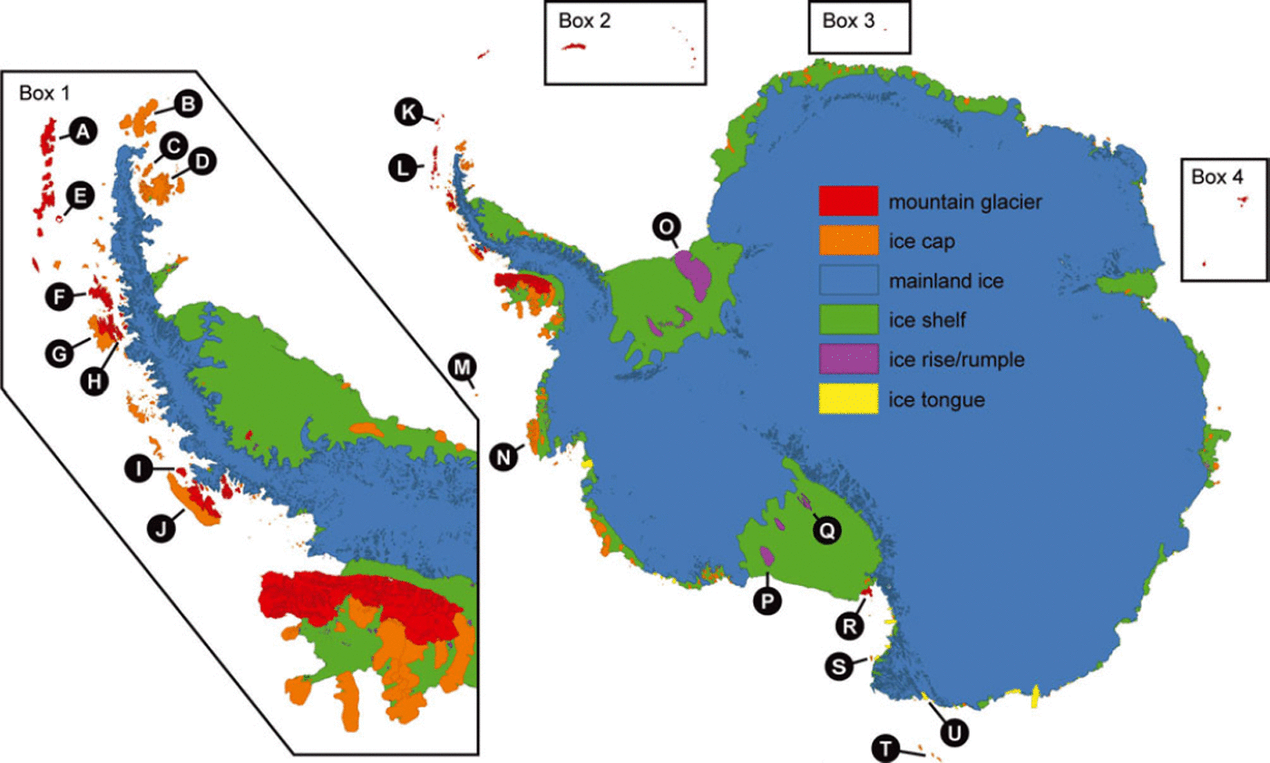
Previous inventories have been limited either in spatial scope or breadth of data. Reference Vinogradov and PsarevaVinogradov and Psareva (1990) compiled a list of Antarctic islands with ice cover, but the list is incomplete and provides little beyond ice area and roughly estimated ice thickness. Reference Rabassa, Skvarca, Bertani and MazzoniRabassa and others (1982) compiled an inventory of James Ross Island and Vega Island, off the northeast coast of the Antarctic Peninsula. Reference Davies, Carrivick, Glasser, Hambrey and SmellieDavies and others (2011) updated the inventory of James Ross Island and added the northern part of the Antarctic Peninsula. The Global Land Ice Measurements from Space project contains only the outlines from Reference Davies, Carrivick, Glasser, Hambrey and SmellieDavies and others (2011) and ice outlines for Kerguelen, and hence covers <3% of all glacier area in the periphery. Drawing on the Antarctic Digital Database (ADD; Reference Fox and CooperFox and Cooper, 1994; ADD Consortium, 2000), Reference Hock, de Woul and RadicHock and others (2009) compiled a 1°x1° grid representing the glacierized areas of the Antarctic periphery. Distinguishing between glaciers and the ice sheet is not straightforward, either conceptually or practically, and depending on the purpose of a study different definitions may be appropriate. Reference Hock, de Woul and RadicHock and others (2009) defined ‘Antarctic periphery’ to include all islands between the mainland coast of Antarctica and the latitude of Kerguelen (49°S), excluding those near New Zealand and the mainland of South America (here we adopt this definition; see red and orange polygons in Fig. 1).
Classification of ice cover based on the Antarctic Digital Database (ADD), including the mountain glacier and ice-cap categories not distinguished in the ADD. Box 1 shows more detail for the Antarctic Peninsula. Boxes 2 (South Georgia and the South Sandwich Islands), 3 (Bouvet Island) and 4 (Kerguelen and Heard Island) are displaced from their proper positions but are at the same scale as the main map. The circled letters correspond to locations mentioned in the text: A. King George Island; B. Joinville Island; C. Vega Island; D. James Ross Island; E. Deception Island; F. Brabant Island; G. Anvers Island; H. Doumer Island; I. Liard Island (Fig. 3); J. Adelaide Island; K. South Orkney Islands; L. South Shetland Islands; M. Peter the First Island; N. Thurston Island (Fig. 2); O. Berkner Island; P. Roosevelt Island; Q. Crary Ice Rise; R. Ross Island; S. Coulman Island; T. Balleny Islands; and U. Znamenskiy Island. Scott Island (67.48 S, 179.98 W) and Marion Island (46.98 S, 37.78 E) do not show up at this scale. The map is drawn on a Lambert azimuthal equal-area projection centred at the South Pole.
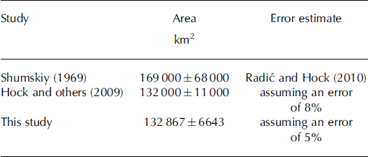
Published estimates of the area of glaciers in the Antarctic periphery vary between 132 000 km2 (Reference Hock, de Woul and RadicHock and others, 2009) and 169 000 km2 (Reference Shumskiy and TolstiikovShumskiy, 1969). Differences are due to different reference dates but also different definitions of the domain. Based on Shumskiy’s 169 000 km2, Reference Radic and HockRadic and Hock (2010) estimated the volume of all Antarctic glaciers as 0.147 ± 0.064 m SLE, representing 25% of global glacier ice volume (excluding the ice sheets). However, uncertainties are large since the estimate was derived by upscaling size distributions of data from the World Glacier Inventory (Reference CogleyCogley, 2008), which covered only a few percent of the glacierized area in the Antarctic periphery. These upscaled Antarctic size distributions were also used in global-scale mass change projections (Reference Radic and HockRadic and Hock, 2011).
Here we compile an inventory of all glaciers in the Antarctic periphery. We distinguish between ice caps (dome-shaped ice bodies with radial flow, largely obscuring the subsurface topography) and mountain glaciers (glaciers that are confined by surrounding mountain terrain; Reference CogleyCogley and others, 2011) and present glacier size distributions, area–altitude distributions, properties related to calving and an updated volume estimate based on volume–area scaling. This dataset has many possible uses. In particular, the improved area estimates and area–altitude distributions will lead to more accurate large-scale mass-balance assessments (of the past) and projections (for the future), since uncertainties are much less than in previous studies. This will also lead to better estimates of the glacier contribution to future sea-level change. Our total volume estimate can serve as a starting point for future volume change predictions. The new inventory could also be used to improve the representation of ice cover in climate models. The inventory shapefiles are available from http://add.scar.org/ and hyp-sometry data are in the supplementary material hosted at http://www.igsoc.org/hyperlink/63a377.html
2. Data and Methods
2.1. Glacier classification
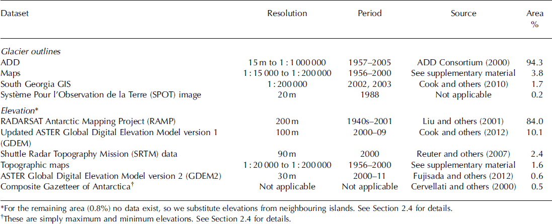
Our new inventory (Fig. 1) is derived from many sources (Table 1). The main source is the ADD (Reference Thomson and CooperThomson and Cooper, 1993; Reference Fox and CooperFox and Cooper, 1994; ADD Consortium, 2000). The ADD presents data at a number of spatial resolutions; we use ‘Scale0’, with the resolution of the best available source material. The data consist of polygons (shapefiles) representing coastlines and rock areas including nunataks south of 608 S. These shapefiles were digitized from paper maps, aerial photos and Landsat, MODIS (Moderate Resolution Imaging Spectroradiometer) and ASTER (Advanced Spaceborne Thermal Emission and Reflection Radiometer) imagery with a range of dates from 1957 to 2005. Coastline polygons are tagged with one of the following surface-type attributes: land (encompassing both grounded ice and rock outcrops), ice shelf, ice tongue and ice rumple. We extract and identify all mountain glaciers and ice caps from the dataset as follows:
Polygons classified as ice shelves, ice tongues and ice rumples are not included in our inventory.
Following Reference Hock, de Woul and RadicHock and others (2009) we exclude all polygons on the Antarctic mainland. Many mainland glaciers resemble mountain glaciers, in particular along the Antarctic Peninsula, and may respond very differently to climate than the large Antarctic ice sheet. However, inspection of satellite images indicated that mountain glaciers on the mainland tend to share boundaries with the ice sheet, making classification difficult and highly subjective.
From the remaining coastline polygons, we erase all rock areas as defined by the rock polygons in the ADD. We assume non-rock areas are ice-covered, thus redefining the land class as a land ice class. The land ice class is further subdivided into ice rise, ice cap and mountain glaciers according to the steps below.
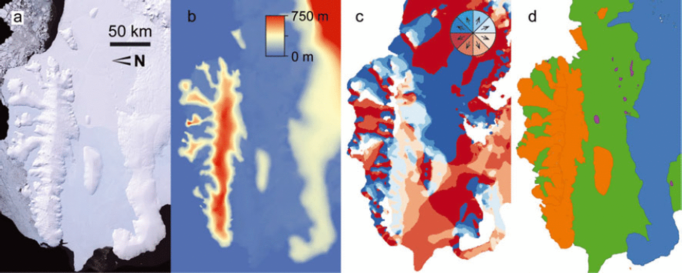
Ice rises, which are excluded from our inventory, are areas in the middle or along the seaward side of ice shelves where the ice impinging on a grounded area appears to flow up and over the bedrock, rather than around it. Usually, ice rises do not have exposed rock nearby and their surface elevations are only slightly higher than the surrounding ice shelf. We used three datasets to identify ice rises (Fig. 2 shows an example). Flow and rock features were examined in Landsat imagery (Reference BindschadlerBindschadler and others, 2008), with a spatial resolution of 15 m. Avelocity map (Reference Rignot, Mouginot and ScheuchlRignot and others, 2011) also helped distinguish local flow around bedrock bumps. It was derived from interferometric synthetic aperture radar (InSAR) data acquired between 2007 and 2009 and optimized for display at the continental scale (spatial resolution 900 m), but it still proved useful for identifying ice rises. If the first two datasets did not yield a clear distinction, we considered the RADARSAT Antarctic Mapping Project digital elevation model version 2 (RAMP DEM; Reference Liu, Jezek, Li and ZhaoLiu and others, 2001). It has a grid resolution of 200m and was constructed from radar altimetry and topographic maps with a variety of scales. Source data spanned the 1940s to 2001, and were mostly from the 1980s and 1990s. We calculated the elevation difference from the summit of each candidate ice body to the surrounding ice shelf. If the difference was <200 m, the ice body was classified as an ice rise. Figure 2 shows examples of these cases.
Although their summits are >200 m above the surrounding ice-shelf surface, we exclude from our inventory all islands in the interior of the Ross, Filchner and Ronne ice shelves (e.g. Berkner Island, Roosevelt Island, Crary Ice Rise).
Ice is classified as mountain glacier if Landsat imagery revealed exposed-rock ridgelines subdividing the ice body. These ice bodies are separated into individual mountain glaciers, as described in Section 2.2. Some of the glaciers thus divided are reclassified as ice caps, based on their morphology.
The remaining land ice bodies are classified as ice caps. Diagnostic features include simple map geometry and ice flow outward from a central high elevation, as seen in the velocity map and RAMP DEM.
Characteristics of the datasets we use to derive glacier outlines and area–altitude distributions. The ADD and RAMP cover a large percentage of the new inventory’s area
Data used in classification for the Thurston Island region (a–c) and resulting surface classification (d), with the same colours as in Figure 1 . (a) Landsat image from the Landsat Image Mosaic of Antarctica. (b) Topography from the RAMP DEM. (c) Flow direction from InSAR. See Figure 1 for location.
For South Georgia, we use ice outlines from the South Georgia GIS (e.g. Reference Cook, Poncet, Cooper, Herbert and ChristieCook and others, 2010). For the other sub-Antarctic islands (Peter the First Island, the South Shetland Islands, the South Orkney Islands, the South Sandwich Islands, Bouvet Island, Kerguelen, Heard Island and the Balleny Islands) we do not use the ADD but manually digitize the outlines of all glaciers, mainly from maps but in some cases from satellite imagery. The total area of these sub-Antarctic islands is 7540 km2, ∼ 6 % of the inventory by area. Ice bodies are classified as ice caps or mountain glaciers following the same criteria as above. The geography of some of the sub-Antarctic islands remains poorly known even today. For example, the best map of the Balleny Islands is an explorer’s sketch, and the islands are not covered adequately by any modern DEM, while maps of the South Sandwich Islands indicate elevations by crude formlines rather than contours.
2.2. Delineation of glacier divides
Where needed, we subdivide the ADD polygons into individual glaciers using a tool for automatic delineation of glacier flow basins (C. Kienholz and others, unpublished information). The tool uses a watershed algorithm commonly available in GIS software to calculate the area that is tributary to a manually defined set of points along each glacier’s terminus (Fig. 3). In practice, the set of points is a segment of the whole polygon, and the end points of the segment are chosen visually. The DEM inputs to the tool are the same as described in Section 2.4. Manual correction of small polygon artefacts is required for some basins.
Data used to create glacier divides for Liard Island (see Fig. 1 for location). (a) Landsat image with the ADD coastline (orange) and manually defined glacier terminus segments (between pairs of green dots). (b) RAMP DEM. (c) Glacier divides from the flowshed algorithm. White areas within the glacier are rock outcrops. The algorithm merged some adjacent glaciers.

Glacier divides on South Georgia are derived from a more automated version of the same GIS tool described above. Where outlet glacier tongues are well defined, the tool is able to choose the terminus end points automatically.
Divides on the remaining sub-Antarctic islands are identified visually, relying on the contours on digitized maps. For some islands the best published maps have no contours; here the mapped ice cover is left undivided.
2.3. Terminus characteristics
A large fraction of the glaciers in our inventory terminate in the ocean, suggesting that frontal ablation (the sum of mass losses by calving and submarine melting) plays a large role in the mass budget of Antarctic periphery glaciers. As a step towards quantifying frontal ablation, we assign all termini to one of five classes: no significant calving; terrestrial ‘dry’ calving; marine calving; lacustrine calving; and drainage into ice shelf. The first four correspond to the classification in Reference CogleyCogley (2008); the last is unique to Antarctica. Classification is done visually using imagery from Google EarthTM (as of 21 March 2012). If more than one category applies to a glacier, it is assigned to the class representing the longest part of its perimeter.
2.4. Hypsometries
Often, mass-balance models are elevation-dependent (e.g. Reference Radic and HockRadic and Hock, 2011) and hence require the area–altitude distribution (hypsometry) of the glacier as input. To calculate hypsometries we primarily use digital elevation data from the RAMP DEM (Table 1). We supplement that source with Shuttle Radar Topography Mission data (Reference Reuter, Nelson and JarvisReuter and others, 2007) for South Georgia, Bouvet Island, Marion Island, Kerguelen and Heard Island. The ASTER Global Digital Elevation Model version 2 (GDEM2; Reference Fujisada, Urai and IwasakiFujisada and others, 2012) covers the South Sandwich Islands and the South Orkneys. An improved version of GDEM (Reference Cook, Murray, Luckman, Vaughan and BarrandCook and others, 2012) covers James Ross Island, the Joinville Islands, Brabant Island, Anvers Island, Adelaide Island and many smaller islands in the vicinity of the Antarctic Peninsula. We calculate the hypsometry of each glacier using 20 m elevation bins.
The RAMP DEM covers King George Island and Deception Island, but for the rest of the South Shetland Islands and Peter the First Island we generate hypsometries from map contours, interpolating to match the 20 m elevation bins of the rest of the dataset.
The remaining glaciers either have no DEM or the GDEM2 is too noisy to use. We assign hypsometries to these glaciers assuming their geometries can be approximated by a circular ice cap (with the measured area) with a surface profile defined by assuming ice to be a perfect plastic with yield stress of 50kPa (Reference Raper and BraithwaiteRaper and Braithwaite, 2006; Reference Cuffey and PatersonCuffey and Paterson, 2010, eqn 8.133). While we use the shape of that surface profile, we adjust the maximum and minimum elevations to match the elevation data available. We take maximum and minimum elevations for the Balleny Islands (Young, Sturge, Buckle and Borradaile) from the Composite Gazetteer of Antarctica (Reference Cervellati, Ramorino, Sievers, Thomson and ClarkeCervellati and others, 2000), a database of place names and mountain peak elevations. The total area of these islands is 661 km2. For islands with no DEM data and no other elevation information, we estimate the maximum elevation based on nearby islands with data. The total area of these 20 islands is 984 km2. Combined, glaciers without DEM data represent only 1.2% of the total area in the inventory (Table 1).
For comparison with other studies, we also calculate synthetic hypsometries for all the glaciers and ice caps in the inventory. For ice caps, we use the formulation described in the previous paragraph. Mountain glaciers typically have the most area in the middle of the glacier’s elevation range. Following Reference Raper and BraithwaiteRaper and Braithwaite (2006), we give the area-altitude distribution a triangular shape, with maximum area at the elevation halfway between the minimum and maximum elevations. To evaluate the appropriateness of these shapes for the Antarctic periphery, we also normalize the elevation and area of each ice body’s hypsometry and calculate the mean shape of all mountain glaciers in the inventory, and, separately, the mean shape of the ice caps.
2.5. Glacier area
We use a GIS to calculate the area of glaciers in the inventory, after projecting the outlines into a Lambert azimuthal equal-area projection centred at the South Pole. Our area estimate contains errors from several sources including the underlying maps and the digitizing process. Reference Fox and CooperFox and Cooper (1994) suggest that individual outlines deviate from their true locations by <300m, and that the total area of Antarctica calculated from the ADD has an error of <3%. The <3% value is based on an earlier estimate by Reference Drewry, Jordan and JankowskiDrewry and others (1982) who report < 1 % error in digitizing paper maps from both machine and operator random errors. Reference Drewry, Jordan and JankowskiDrewry and others (1982) estimate the total area error to be <3% due to the quality of underlying maps, and highly mobile boundaries in many areas. It is difficult to evaluate the error of the underlying maps, without expending considerable effort to create independent outlines from satellite imagery. Reference Hock, de Woul and RadicHock and others (2009) estimate area for the Antarctic periphery using the GGHYDRO 2.3 global hydrographic dataset (Reference CogleyCogley, 2003), which gives the percentage of glacierization in a 1° x 1° global grid. They adopted Cogley’s single-cell accuracy error estimate of 8% for the error of the total area. The definition of the domain - whether to count certain ice bodies as part of the periphery-also impacts the total area estimate, but we do not consider this in our error estimate. Lacking detailed information for a more rigorous approach, here we assume a 5% error for the total area of our inventory (in line with, e.g., Reference Paul and AndreassenPaul and Andreassen, 2009; Reference Bolch, Menounos and WheateBolch and others, 2010).
2.6. Glacier volume
Total ice volume was computed using volume-area scaling (Reference Bahr, Meier and PeckhamBahr and others, 1997):

where Vis the volume and A the area of a single glacier and c and 7 are scaling parameters. Following Reference Radic and HockRadic and Hock (2010) we use c= 0.2055 m3 - 2 7 and 7 = 1.375 for mountain glaciers in the inventory. Assuming a parabolic form of thickness-length relation, the volume of each ice cap is computed using c= 1.7026 m3–27 and 7 = 1.25. We calculate the error of volume using error propagation for the equation above, assuming random independent errors for each term. We assume the error in each glacier’s area is 5%. Following Reference Radic and HockRadic and Hock (2010), we assume ± 4 0% error in c and ±0.015 error in 7.
For comparison, we calculate volumes from the BEDMAP ice thickness dataset (Reference Lythe and VaughanLythe and others, 2001) for 157 of the largest glaciers in the inventory. All these glaciers are larger than 50 km2 and they account for ∼ 9 0% of the inventory’s total area. BEDMAP is constructed from airborne and ground-based radar surveys, seismic reflection and gravity measurements. BEDMAP has a coarse grid resolution (5 km), and the data that went into it are quite sparse for some glaciers, but it is currently the best available ice thickness dataset that covers the area of the inventory. Reference Lythe and VaughanLythe and others (2001) estimate the root-mean-square error of grid elevations for the Antarctic Peninsula to be 163 m, which we apply to all gridcells for our error analysis. We use volume-area scaling to fill in the volume of glaciers not covered by BEDMAP. The scaling parameters are tuned to match the BEDMAP measurements with no distinction between mountain glaciers and ice caps: c= 0.2187m3–27 and 7 = 1.341.
3. Results and Discussion
3.1. Number and area of glaciers
In total we identify 1133 ice caps covering 91042 ± 4552 km2 and 1619 mountain glaciers covering 41 825 ±2091 km2. Hence our glacier inventory includes 132 867 ± 6 6 4 3 km2 of ice on Antarctic and sub-Antarctic islands. Our estimate of the total area of glaciers in the Antarctic periphery is similar to that of Reference Hock, de Woul and RadicHock and others (2009; Table 2). This is not surprising as they also used the ADD as a basis for their study. The difference is due to slightly different definitions of the domain, mainly with regard to ice rises. Our estimate is less than that of Reference Shumskiy and TolstiikovShumskiy (1969), whose methods are not explained and are thus not reproducible. We also made an independent estimate of area using island coastlines extracted from the MODIS Mosaic of Antarctica (Reference Scambos, Haran, Fahnestock, Painter and BohlanderScambos and others, 2007), again excluding the large islands in the Ross and Ronne-Filchner Ice Shelves. The resulting area, 132 272 km2, is close to the estimate from our new inventory, giving us confidence in our area estimate.
Area of Antarctic periphery glaciers, as estimated in different studies
Our estimate for number of glaciers must be treated with caution since it strongly depends on the definition of an individual glacier. Separating contiguous glaciers is complicated in the Antarctic periphery. Indeed, it is often a matter of subjective judgment. Some ice bodies resembling ice caps have pronounced outlet glaciers; their longitudinal profiles are convexo-concave, unlike the convex-up profiles of ice caps with well-developed domal morphology or the concave-up profiles of many mountain glaciers. Our classification does not contain a separate class of outlet glaciers, nor does it rest on an objective criterion for distinguishing between ice caps and mountain glaciers. Nevertheless, our estimate combined with the area of each ice body provides a first approximation for studies applying volume–area scaling for assessments of ice volume or projections of mass changes. For these purposes, the power law that relates volume to area requires that the area of each individual glacier, or at least the frequency distribution of glacier sizes, be known.
3.2. Size distribution
Figure 4 shows the size distribution of all glaciers in the inventory. Glacier sizes range from 0.01 to 6000 km2. The eight largest glaciers in the inventory (>3000 km2 each) cover 25% of the total area. Most of the glaciers larger than 100 km2 have a surface morphology that led us to classify them as ice caps. In some cases, a single island has more than one ice cap. There are more mountain glaciers than ice caps for areas between about 0.5 and 100 km2. The inventory contains a large number of small (<1 km2) ice-covered islands, most of which are observed to have an icecap morphology, but their combined area is only 359 km2.
Histogram showing the size distributions of ice caps and mountain glaciers in the new inventory: (a) number of glaciers and (b) fraction of total area per size bin of 0.2 log10 (km2) vs area. The bars are stacked.

3.3. Terminus characteristics
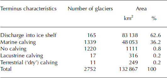
More than 99% of the glacierized area drains through marine-terminating termini or into ice shelves (Table 3). In terms of area (and implicitly volume), more of the ice from the peripheral islands is discharging into ice shelves than directly into the ocean. By number of glaciers, marine calving is the most common style, but this category includes many small islands, so the total area is less than for ice shelves. Some of the marine-calving termini are of classical type, with glacier ice standing in water, but a common form of terminus is one in which the glacier ends either at the high-water mark or sufficiently close to it that calved ice may float away. An example is the Costa Recta on Deception Island, illustrated by Reference Lopez-Martinez, Serrano and SmellieLopez-Martinez and Serrano (2002). Over 1200 glaciers end on land with no significant calving; these glaciers also tend to be small. The terrestrial calving glaciers, found only on Coulman Island, Znamenskiy Island and Bouvet Island, usually end above rocky bluffs, such that the calved ice quickly falls into the ocean, but the ocean does not contact the glacier. Of glaciers calving into lakes, there is one on Signy Island in the South Orkneys, six on Kerguelen and four on South Georgia. There are also three glaciers terminating in coastal freshwater lagoons on Heard Island and three more on South Georgia. Except for Ampe`re Glacier on Kerguelen (Reference Berthier, Le Bris, Mabileau, Testut and RemyBerthier and others, 2009), there is no information on the significance of lacustrine calving as a component of the mass budget of these glaciers.
Terminus characteristics of Antarctic periphery glaciers
3.4. Hypsometries
Altitudes of all glaciers in the inventory range from 0 to 3600 ma.s.l. The highest point in the region is on Mount Erebus, Ross Island. By numbers, 66% of the glaciers terminate within 50 m of sea level. Approximately 94% of the glacierized area in the Antarctic periphery is within 1000 m of sea level, and 74% is within 500m (Fig. 5a). Ice caps have 88% of their total area below 500 ma.s.l. while the corresponding number for mountain glaciers is 44% (Fig. 5b). Above 1000m a.s.l., ice caps have only 1584 km2 (2% of their total area), while mountain glaciers have 6858 km2 (16%). Mountain glaciers tend to have a larger proportion of their area at higher elevations, because the ice is partially supported by drag along valley walls (Reference Cuffey and PatersonCuffey and Paterson, 2010) and the confining walls are not conducive to the ice-cap morphology.
(a) Cumulative area with increasing elevation. (b) Combined hypsometry for all glaciers and ice caps in the inventory, with 20m elevation bands. Solid lines show the hypsometry calculated from DEM data; dashed lines show the synthetic hypsometry calculated just from maximum and minimum elevations of individual ice bodies. The DEM hypsometry has spikes every 250m as a result of imperfect interpolation when the RAMP DEM was created from map contours.
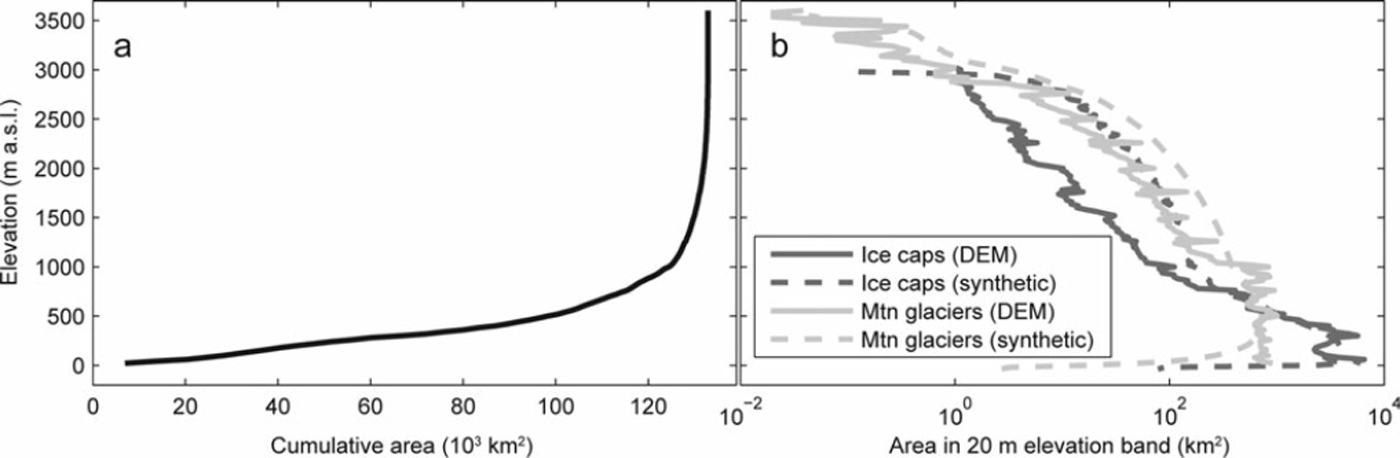
Due to lack of inventory data, Reference Radic and HockRadic and Hock (2011) used synthetic hypsometries and glacier areas to model future glacier response to climate change. The synthetic hypsometries we calculate for our inventory make use of the maximum and minimum elevation data that we generate, so they are an improvement over Reference Radic and HockRadic and Hock (2011), but still do not exactly match the DEM-derived hypsometries (Fig. 5b). Within 1000 m of sea level, the measured ice-cap hypsometries have 6% more area than the synthetic (23% for mountain glaciers). Above 1000 m, the synthetic hypsometries have 4.2 times more area than the DEM-derived hypsometries for ice caps (2.2 times for glaciers). The greater frequency of high elevations in the synthetic dataset would bias the results of mass-balance modelling towards higher values.
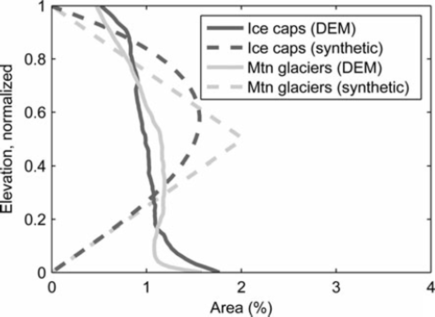
The mean shape of the normalized measured hypsom-etries is considerably different from the standard synthetic hypsometries (Fig. 6). The observed hypsometries of mountain glaciers and ice caps are similar. Both have a relative excess of area in the lowest 20% of the elevation range, fairly constant area between 20% and 90%, and diminishing area above 90%. The extra area at low elevation is often an ice piedmont – where a glacier flows out of the mountains onto a coastal plain. The reduced area at high elevations is a function of steep mountain topography in the glacier case, or the small radius of the summit of an ice cap. Antarctic glaciers differ from the patterns assumed by Reference Raper and BraithwaiteRaper and Braithwaite (2006), perhaps because many terminate in the sea, instead of on land as would be typical of glaciers elsewhere in the world.
Normalized hypsometries averaged over all ice caps and mountain glaciers based on DEMs and synthetic hypsometries following Reference Raper and BraithwaiteRaper and Braithwaite (2006). There are 100 elevation bins, so a rectangular sloping plane would plot as a vertical line at 1%.
3.5. Glacier volumes
Our best estimate of total glacier volume for the Antarctic periphery is 48 636 ± 3849 km3 , corresponding to 0.121 ± 0.010 m SLE. We assume a glacier density of 900 kg m–3 and an oceanic area of 3.625 x 10⁸ km2 (Reference CogleyCogley, 2012). The total volume is the sum of 17428 ± 2254 km3 in glaciers and 31 208 ± 3121 km3 in ice caps. If all the ice bodies were ice caps, volume-area scaling would give 42194 km3. If they were all mountain glaciers, the volume would be 72297 km3. Using the BEDMAP thickness data, we find a volume of 38869 ± 2639 km3. We consider the BEDMAP volume to be an underestimate because ice thickness measurements are sparse while rock outcrops (assumed to have zero ice thickness) are completely mapped. Our volume estimates correspond to a domain-average thickness (total volume divided by total area) of 417 m for mountain glaciers and 343 m for ice caps. Mean thicknesses differ for glaciers and ice caps due to different parameters in the scaling relationship.
Our best volume estimate is 18% lower than the estimate by Radic and Hock (Reference Radic and Hock2010; 59521 ± 25829 km3), largely because of our 21 % lower area estimate. Additionally, unlike Radic and Hock, we know the number of glaciers in different size ranges. Our error estimate has been reduced accordingly.
4. Conclusions
Our new inventory of Antarctic periphery glaciers contains 132867 ± 6643 km2 of ice. The inventory includes grounded ice that is separated from the mainland by open water or ice shelf, but does not include the islands contained within the Ross and Filchner-Ronne Ice Shelves. We have classified ice bodies by their morphology (ice cap vs mountain glacier). Based on volume-area scaling, we estimate the ice volume in the Antarctic periphery to be 48636 ± 3849 km3. We find that 63% of the glacier area in the inventory discharges into ice shelves, while 36% calves ice directly into the ocean. The remaining 1 % terminates either on land or in a lake. In contrast to glaciers in other regions, we find that Antarctic glaciers tend to have a rather uniform distribution of area across elevations, but a disproportionately large fraction in the lowest 10% of their elevation range. The inventory is available on the ADD website (http://add.scar.org). The associated hypsometry files and a list of data sources used are in the supplementary material at http://www.igsoc.org/hyperlink/63a377.html
The inventory is a major advance over what was previously available. Further improvements to the inventory could be made by digitizing a consistent set of outlines from satellite imagery. A time series of outlines would allow studies of glacier change. To improve the hypsometries, better DEMs are needed. Careful separation of adjacent glaciers will increase the accuracy of volume estimates from volume–area scaling. Additional ice thickness measurements from the peripheral islands are needed to better estimate the total ice volume and validate the volume–area scaling results.
Acknowledgements
This work was supported by grants from NASA (NNX11AO23G) and the US National Science Foundation (ANT-1043649). We thank Christian Kienholz for providing his glacier delineation code and assisting with its application, Justin Rich for providing code to calculate hypso-metries, and Valentina Radic for helpful discussions.



