Nomenclature
- b
-
span (m)
- c
-
chord (m)
-
 ${C_D}$
-
drag coefficient
-
${C_d}$
-
sectional drag coefficient
-
${C_{DS}}$
-
drag coefficient due to suction system
-
${C_L}$
-
lift coefficient
-
${C_l}$
-
sectional lift coefficient
-
${E^*}$
-
energy density (Wh/kg)
- g
-
gravitational acceleration (m/s
$^2$
) - J
-
fitness function
-
${C_L}/{C_D}$
-
lift-to-drag ratio
-
$m$
-
mass (kg)
- P
-
power (W)
- R
-
range (km)
- Re
-
Reynolds number
- t
-
thickness
- W
-
weight (kg)
-
$W/S$
-
wing loading (kg/m
$^2$
)


Greek symbol
-
$\alpha $
-
angle-of-attack
-
$\Lambda $
-
wing quarter-chord sweep
-
${\eta _{{\rm{t}}otal}}$
-
total efficiency


Subscripts
- b
-
battery
- r
-
root
- t
-
tip
- TO
-
take-off
- w
-
wing
Abbreviations
- AR
-
aspect ratio
- ATTAS
-
Advanced Technologies Testing Aircraft System
- BLS
-
boundary layer suction
- CFD
-
computational fluid dynamics
- HLFC
-
hybrid laminar flow control
- IV
-
improved Van Ingen method
- LFC
-
laminar flow control
- LST
-
linear stability theory
- MDO
-
multidisciplinary design optimisation
- MTOM
-
maximum take-off mass
- MTOW
-
maximum take-off weight
- NLF
-
natural laminar flow
- TLR
-
top-level requirement
1.0 Introduction
The aviation industry is facing one of the new challenges of the XXI century: significant reduction of environmental impact without preventing people and goods from travelling worldwide. Last years have been characterised by a substantial increment of passengers and goods flying, as shown by the 2019 analysis of the Bureau of Transportation Statistics, even the world financial crisis in 2008 had only a temporary effect on aviation, after which a growing trend was established again. In Flightpath 2050Footnote 1, authorities set challenging goals like the reduction of 75% of CO2 and 90% of NOx emission. In the German research Cluster of Excellence SE2A (Sustainable and Energy Efficient Aviation), a combination of technologies for the design of future transport aircraft is being investigated. The technologies under study to understand the possible benefits are: electric propulsion systems for regional aircraft, load alleviation, novel structures and materials, active flow control.
Aircraft electrification may help in reaching the cited goals by 2050. At the present moment, electrification has entered the market of the General Aviation sector and Light Sport Aircraft due to the lower battery energy and electric motor power densities required. The fully electric 600kg maximum take-off mass (MTOM) “Velis Electric” by Pipistrel [1], EASA certified, has given further interests to similar companies to develop airplanes with electric propulsion. The propulsion system manufacturer MagniX has introduced an all-electric propulsion system and first retrofitted De Havilland Beaver and then 208B Cessna Grand Caravan. The electrified Caravan became the largest all-electric aeroplane of recent times [2]. Airbus has developed an experimental all-electric E-fan aircraft to study the capabilities of an electric aircraft [Reference Jackson3]. In particular, the E-fan concept had multiple versions, from a technology demonstrator to a production variant. In this background, great interest is shown to develop a new integrated software framework for preliminary aircraft design. The main focus is on integrating and evaluating (hybrid) electric propulsion concepts [Reference Aigner, Stumpf, Hinz and De Doncker4]. However, to realize electrification on a larger scale, for example, in regional aircraft, the electric propulsion should be combined with some novel airframe technologies such as active flow control, active load alleviation, and novel structures and materials. This integration seems necessary since an additional reduction in aircraft structural weight and aerodynamic drag is required due to insufficient battery energy density for larger aircraft.
Load alleviation introduces various techniques to reduce the bending moment experienced by the aircraft, and hence significant structural weight reduction, via passive or active approaches. Reduction of maximum bending moment enables the design of lighter wings for lower limit load factors. Passive load alleviation solutions consider nonlinear stiffness material design [Reference Horst, Elham and Radespiel5], viscoelastic damping design [Reference Gröhlich and Böswald6], new structural concepts [Reference Dähne and Hühne7, Reference Wunderlich, Dähne, Reimer, Schuster and Brodersen8], and local morphing structures [Reference Horst, Elham and Radespiel5]. Nonlinear stiffness materials may improve the load distribution on the wing under low load cases (0.5–1.5g) and improve performance and efficiency at those load cases. Viscoelastic damping composites characterising by the viscoelastic layer can be used for shear deformations under vibration loads due to gusts or flight manoeuvres. Consequently, some vibration energy is dissipated so that the structure can be designed for lower limit loads. Finally, both aeroelastic tailoring and local morphing structures aim to extend the aeroelastic design space. Morphing is introduced to deliberately have deformations of the wing like its torsional rotation to reduce the effective angle-of-attack. Another suitable approach is to change aerofoil shape for load reduction [Reference Horst, Elham and Radespiel5]. The wing active load alleviation uses different types of flow control over the wing to achieve a more favorable wing load distribution and reduce the wing bending moment. Previously, researchers have approached the design of active load alleviation systems in different ways. Rossow et al. [Reference Rossow, Geyr and Hepperle9] investigated the feasibility of an aircraft featuring load alleviation technologies; Liu et al. [Reference Liu and Sun10] looked at active load alleviation from the control system perspective. Finally, active load alleviation could also be reached by fluidic or micro-mechanical flow actuators that change the load distribution along the wing and reduce the bending moment [Reference Khalil, Asaro and Bauknecht11].
Novel structural concepts and materials are being developed to improve the aircraft structure in terms of stiffness and weight. Bishara et al. [Reference Bishara, Horst, Madhusoodanan, Brod, Daum and Rolfes12] describe advanced structural design with the integration of active flow control, which is directly applicable to the presented work. Additional information regarding the structural layout of the wingbox with HLFC system is described in [Reference Horst, Elham and Radespiel5]. Moreover, the potential use of thin ply materials for novel airplanes was also considered in [Reference Horst, Elham and Radespiel5].
Boundary layer suction (BLS), as explained in detail in Section 2, represents a way for aircraft drag reduction. The earliest known experimental work on Laminar flow control (LFC) on aircraft was done in the late 1930s, primarily in wind tunnels [Reference Braslow13]. Laminar flow can be passively obtained over the forward part of airplane lifting surfaces by designing surface cross-sectional contour. The local pressure initially decreases over the surface in the direction from the leading edge towards the trailing edge (for leading-edge sweep angles of less than 18 degrees). These kinds of aerofoils are called natural laminar flow (NLF) aerofoils. In the rearward region of wings, pressure increases towards the trailing edge, developing an adverse pressure gradient which stimulates boundary layer instabilities that lead to the boundary layer transition. Hence, active laminar flow control has to be used to further extend the surface laminar flow. Researchers in Northrop Corporation in the 1950s developed a method of analyzing cross-flow instability due to sweep, and some experimental data showed the possibility to control this kind of instabilities by a reasonable amount of suction. The continuous suction demanded by LFC imposes penalties in weight, systems complexity, and operational compromises, thus reducing the practical benefits in drag reduction. Since the mid-1980s, most of the research was focused on hybrid laminar flow control (HLFC) [Reference Krishnan, Bertram and Seibel14]. Boeing has already implemented a passive HLFC system. The 787-9 represents their first model to be equipped with HLFC, which is a feature of its on the horizontal and vertical tails, benefits are stated as “significant” [Reference Spalart and McLean15]. Airbus conducted different flight tests on the vertical tailplane of A320 to assess the advantages of the HLFC, subjected to simplifications under the ALTTA project [Reference Schrauf and von Geyr16]. The Faculty of Aerospace Engineering of the Delft University of Technology acquired an Euro-ENAER EE–10 Eaglet, a two-seat monoplane characterised by full composite airframe structure, 850kg MTOM. The main purpose is to use the model for research, in particular on flow laminarisation. Some preliminary results, considering the BLS technology, have shown the necessity of designing a new aerofoil optimised for active flow control. The new wing proved a drag reduction of 13% at cruise [Reference van de Wal17]. Recent work by Beck et al. [Reference Beck and Landa18] suggested that an overall fuel burn reduction of 47% can be attained by fully utilising the potential of boundary layer suction (BLS) for a midrange aircraft configuration. The study used a forward-swept wing configuration with an 80% laminar flow wing and a 70% laminarised fuselage. Karpuk et al. performed an aircraft design and performance analysis for a blended wing body configuration with BLS [Reference Karpuk, Yaolong and Elham19]. They used multi-fidelity aircraft design code SUAVE with a connection to high-fidelity computational fluid dynamics (CFD) code SU2 but simulating the active flow control with low-fidelity model. Different works are characterised by aerofoil shape optimisation with BLS [Reference Buckley, Zhou and Zingg20, Reference Gardner and Selig21], while other studies investigate the control of boundary layer suction [Reference Zhao, Wang and Cao22, Reference Nelson, Wright and Rioual23]. Sudhi et al. performed a 2D optimisation for aerofoil shape design to minimise drag and power absorbed by BLS for a subsonic un-swept wing [Reference Sudhi, Elham and Badrya24]. The HLFC-optimised aerofoil, with onset suction fixed at 50%, gives a parasite drag reduction of 31%.
The present work aims to provide a physics-based multidisciplinary design optimisation (MDO) of the reference aircraft designed in SE2A. The aircraft is a short-range passenger aircraft with fully electric propulsion, equipped with BLS on the upper lifting surfaces and full fuselage, load alleviation on the wing, and novel structures and material for the whole aircraft structure. The main focus of this work is on physics-based simulation of BLS in an MDO framework for wing aerostructural design. The present work is divided into several sections. Section 2 focuses on active flow control, while Section 3 represents the conceptual aircraft design, starting point for multiple initial data used in this research. Section 4 clarifies the multidisciplinary design optimisation characteristics like the design vector or the fitness function and all the elements necessary to fully understand the optimisation studied. In Section 5 detailed steps of the framework are shown. Section 6 presents all the results from the optimisation and precious information for the current category of aircraft design. Finally, in the last section, conclusions are presented.
2.0 Active flow control: Boundary layer suction
2.1 Flow physics
In 1904, Prandtl [Reference Tollmien, Schlichting, Görtler and Riegels25] conceptualised that the flow over a body has a thin region attached to the surface called boundary layer, where the viscous effects are dominating. The flow near the surface is brought to rest, developing a velocity gradient until the edge of the boundary layer, where the flow is inviscid. The turbulent boundary layer has steeper velocity gradients near the wall, resulting in higher skin friction drag. The increased boundary layer thickness also increases the displacement of the external flow, resulting in a marginal increase in pressure drag. Re
 $_{{\rm{i}}nd}$
is defined by Schlichting [Reference Schlichting and Gersten26] as the minimum Reynolds number below which instability does not rise. The developing boundary layer is subjected to external disturbances due to receptivity and initiates the transition process [Reference Morkovin27] as they excite disturbance waves. These disturbance waves superimpose the laminar base flow and become unstable at R
 $_{{\rm{i}}nd}$
. The amplification of these disturbance waves in the primary instability mechanism can be theoretically modelled by linear stability theory.
 ${e_N}$
method [Reference Van Ingen28, Reference Smith29] is a semi-empirical approach using linear stability theory to analyse the stability of a laminar boundary layer by superimposing harmonic oscillations as small disturbances on an otherwise steady flow. The amplification of these disturbances downstream at a station x is denoted by an amplification factor, called N factor as defined as
 \begin{align*}N = ln\frac{a}{{{a_o}}} = \int_{{x_o}}^x {a_i}dx \end{align*}
where
 ${x_o}$
is the station where the disturbance with frequency
 $\omega $
and amplitude
 ${a_o}$
first becomes unstable. The method uses a database of the frequency response of the instabilities linked to the state of the boundary layer. It does not model the physics of the boundary layer transition. However, as the growth of disturbances from
 $N = 0$
to
 $N = 7$
is linear, a large part of the amplification dominated by Tollmien – Schlichting instabilities (TSI) is predicted very well by the
 ${e_N}$
method. Extrapolation to the non-linear interactions of the disturbance, is only necessary for a short region (
 $N \gt 7$
) of the N factor growth curve due to its exponential nature. Flow is predicted to transition to turbulent flow when the N factor reaches a critical value called
 ${N_{{\rm{c}}rit}}$
.
Critical N Factor and Effect of BLS on TSI

The value of
 ${N_{{\rm{c}}rit}}$
is experimentally validated and differs with receptivity factors.
 ${N_{{\rm{c}}rit}}$
value of 13 is used in this study for flight conditions based on the in-flight experiments conducted with DLR flying testbed ATTAS (Advanced Technologies Testing Aircraft System) [Reference Redeker, Horstmann, Koester, Thiede and Szodruch30, Reference Horstmann, Redeker, Quast, Dressler and Bieler31]. N-factor identification was performed using a specially designed wing glove with modified sections. Linear stability analysis delivered amplification rates for cross-flow instabilities (CFI) and TSI. The measured transition locations from the same experiment were used to correlate the envelopes of
 ${N_{{\rm{T}}S}}$
and
 ${N_{{\rm{C}}F}}$
, as shown in Fig. 1(a). The exact values of
 ${N_{{\rm{c}}rit}}$
is then taking into account the desired transition location for the range of application of the present research, in particular same value has been chosen for parallel studies inside the SE2A Cluster that can be found in [Reference Beck and Landa18, Reference Sudhi, Elham and Badrya24].
2.2 Aerodynamic solver and transition prediction
Flow transitions from laminar to turbulent flow due to the amplification of instabilities. Three sources of instabilities occur on the wing during flight: (1) Tollmien – Schlichting instabilities (TSI), (2) cross-flow instabilities (CFI), and (3) attachment line instabilities (ALI). Boundary layer suction is an approach towards dampening the growth of these instabilities. The transition to turbulent flow is delayed by removing a small portion of the boundary layer near the wall as shown in Fig. 2. This suction also helps to maintain a stable shape factor for the velocity profile and delays separation. By introducing wall-normal velocity to the Prandtl boundary layer equation, suction velocities necessary to laminarise a flow are derived. For a flat plate, the non-dimensionalised suction velocity is given by [Reference van de Wal17]
 \begin{align}\frac{{{v_o}}}{{{U_\infty }}} = \frac{1}{{0.2205}}\frac{1}{{\dfrac{U}{{{U_\infty }}}}}\frac{{d\left(\dfrac{U}{{{U_\infty }}}\right)R{e_\theta }}}{{d\left(\dfrac{x}{c}\right)R{e_c}}} \end{align}
Schematic representation of boundary layer suction [Reference Boermans32].

A modified solver based on XFOIL [Reference Drela33] with the integration of a full
 ${e_N}$
method called XFOILSUC [Reference Bongers34, Reference Ferreira35, Reference Broers36] is used for the aerofoil design. XFOILSUC is a panel-based code that is well suited for the design and analysis of subsonic aerofoils and is computationally inexpensive for performing design optimisation compared to high-fidelity CFD solvers. The original
 ${e_N}$
envelope method used for transition prediction in XFOIL predicts the N factor growth based on a linear approximation of the envelopes of the spatial amplification curves and was derived for self-similar Falkner-Skan laminar boundary velocity profiles [Reference Drela33]. This approach, however, cannot predict the damping of T-S waves due to BLS. XFOILSUC has an improved transition prediction capability coupled to the integral boundary layer solver along with a suction boundary condition. A new database full
 ${e_N}$
transition prediction method called improved Van Ingen method (IVI) [Reference Van Ingen37, Reference Van Ingen38] is used in XFOILSUC. IVI method can predict N factor damping due to BLS, as seen in Fig. 1(b). This method can track the amplification and damping of 601 frequencies logarithmically spaced values between 10
 $^{ - 7}$
and 10
 $^{ - 1}$
, based on the stability data from Arnal datasets [Reference Arnal39]. Inside the SE2A Cluster, a series of 2D optimisations are performed to deisgn the aerofoil able to maintain a low drag with a low power suction absorption for boundary layer suction. These optimisations were done for different Cl and onset of suction and resulted in the SE2A HLFC aerofoil. One of the optimisations useful for the HLFC aerofoil was set for Cl = 0.4, Re = 16 M,
 $M = 0.4$
with no limits of the extension of the laminar flow. Accuracy of XFOILSUC in predicting the flow and transition behaviour is compared with the Reynolds Averaged Navier Stokes solver TAU in Fig. 3.
Comparison between XFOILSUC and TAU [Reference Sudhi, Elham and Badrya24].

The shape factor and friction coefficient are in good agreement, especially until 80% of the chord. However, TAU predicts a transition at 83% while for XFOILSUC transition happens at 85% of the chord. The N factor amplification predicted by XFOILSUC shows similar behaviour as the envelope of instability amplifications calculated by linear stability theory (LST) using the boundary-layer code COCO-LILO [Reference Schrauf40]. XFOILSUC is based on the Arnal stability diagrams while LILO uses non-local linear stability analysis by solving the Orr-Sommerfeld equation. It is solved thanks to boundary layer profiles calculated by COCO for a range of frequencies. The possible difference given by XFOILSUC in the estimation of transition and hence drag respect to higher fidelity tools, is considered as acceptable, in particular considering the interest in studying the possible changes in the transition line with the use of suction. A solution to avoid the possibility of calculation of transition and aerodynamic parameters over a separation bubble that may lead to inaccuracies is to use a forced transition. In this research, optimised results are aerodynamically tested for forced transition at 80% chord, and they show a limited drag difference keeping the optimised results for free transition more conservative and fundamental to understand the shifting of the transition point.
Aircraft sizing procedure from PyInit within SUAVE.

3.0 Conceptual aircraft design
In the German Cluster of Excellence
 $S{E^2}A$
(Sustainable and Energy Efficient Aviation), conceptual design of a short-range full-electric aircraft equipped with BLS, passive and active load alleviation as well as novel materials and structures is considered. The top-level requirements of this aircraft are defined similarly to ATR-72 aircraft, however, with an increase in the number of passengers to 100. The initial sizing of the aircraft is done using an in-house Python software: PyInit. The design process is shown in Fig. 4, connecting PyInit and SUAVE [Reference Lukaczyk, Wendroff, Colonno, Economon, Alonso, Orra and Ilario41]. In particular, PyInit is automating preliminary design performed traditionally by using Excel spreadsheets. Hence, it includes various semi-empirical and physics-based formulations for aerodynamic design and analysis, static stability and control, propulsion, landing gear sizing and flight performance characteristics. The methods were obtained from [Reference Raymer42, Reference Gudmundsson43, Reference Torenbeek44, Reference Roskam45]. First, the initial constrained analysis of the aircraft concept was performed to meet the top level requirements. Then, based on semi-empirical weight formulation and obtained wing loading and thrust-to-weight ratio, the aircraft wing and empennage were sized. Based on the initial sizing, initial geometric components such as the wing aspect ratio, sweep, taper and the tail volume ratios were imported into SUAVE as constant inputs. Also, the power-to-weight ratio and the wing loading were imported as constants. Finally, based on initial range analysis, the maximum range cruise speed was determined and imported into SUAVE as the cruise speed for further sizing. OpenVSP [Reference McDonald46] and CATIA were used for the aircraft geometric modelling.
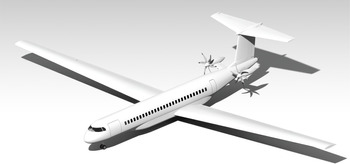
Table 1 synthesizes initial data related to the geometry of the aircraft, shown in Fig. 5.
Regional electric aircraft initial geometric data

Short range aircraft configuration.

In the conceptual design phase, the influence of these novel technologies is considered using low-fidelity methods. Laminar flow control is estimated by modifying the flow transition location along with the wing profile, the active load alleviation effect is assessed by reducing the aircraft limit load factor from the required 2.5Footnote 2 to 2.0. Finally, the use of novel materials is taken into account considering a 15% wing weight reduction compared to aluminium structures. In particular, they are obtained according to the analysis above explained and updated according to the latest developments in the Cluster of Excellence research. In the present work, two different optimisations are studied with two different aerofoils: NACA 65(2)415 and the HLFC
 $S{E^2}A$
Aerofoil designed in the Institute of Fluid Mechanics, Technische Universität Braunschweig under a research process for hybrid laminar flow control (HLFC) aerofoils, further details can be found in [Reference Sudhi, Elham and Badrya24]. The
 $S{E^2}A$
aerofoil has been mainly studied for design
 ${C_l}$
range between 0.3 and 0.7, Reynolds number of 16 million and a Mach number of 0.4 [Reference Sudhi, Elham and Badrya24]. Different scenarios were simulated, in particular with onset suction variation. In Fig. 6 the two aerofoils with BLS present a similar behaviour for the design range. The two aerofoils are tested with suction on the upper surface and fixing transition at 80% for the given range of
 ${C_l}$
. The optimised SE2A HLFC aerofoil presents a lower drag, in detail, an extension of the drag bucket is visible. For a higher value of lift coefficient, the transition is shifted towards the leading edge producing the kink in the plot. Besides, the angle-of-attack is incremented and for these high
 ${C_l}$
values XFOILSUC is more subject to convergence issues. For the defined range the lower surface of the HLFC aerofoil is experiencing natural laminar flow from 70% to 77%, for a
 ${C_l} \lt $
0.3 the transition moves forward producing a kink in the curve, in fact the pressure distribution on the surface makes the aerofoil being mostly turbulent for such low values of lift coefficients. Pressure coefficient and specific power data are obtained for
 ${C_L}$
0.4 and Mach 0.4. The
 $S{E^2}A$
aerofoil permits to save almost 20W/m2 of power for BLS. The promising results presented in the 2D analysis makes the comparison interesting for a complete wing study like this research.
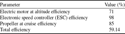
The electric propulsion system efficiencies are reported in Table 2, the total efficiency is the product of the three different efficiencies considered: electric motor, electronic speed controller (ESC) and propeller efficiency. It can be noticed that the final value 59.14% is mainly influenced by the electric motor efficiency, which low value is driven by the cruise altitude.
The scenario studied in the present work is characterized by a cruise-flight at 6,096m of altitude, Mach = 0.383, and airspeed 121m/s. Range, considered a top-level requirement, is computed from initial data in Table 1 and energy network parameters in Table 2, with the Breguet ‘modified’ formula [Reference Hepperle55]. The design range, including reserve, is
 $1,286$
km.
Electric propulsion efficiencies

NACA 65(2)415 and HLFC SE2A aerodynamic characteristics comparison.

4.0 Multidisciplinary design optimisation
4.1 Definition of the problem and design variables
The application of BLS drastically changes the friction drag of a wing. Therefore, the optimal geometry of the wing will be influenced by this technology. Besides, since the total value of the aerodynamic drag is reduced, the balance between the aerodynamic drag and structural weight of the wing is influenced, so a new optimal point is expected as the compromise between drag and weight. In this section, an aircraft wing MDO is presented to investigate the influence of the BLS on wing design. To achieve this goal, physics-based methods for aerodynamic analysis and structural weight estimation are implemented.
For the full electric aircraft, the aircraft maximum take-off weight (MTOW) is used as the objective function. The root and tip aerofoil shapes are fixed. The maximum thickness to chord ratio at the two different positions is scaled and used as design variables. Besides, geometric parameters like span, sweep angle with respect to the leading edge, chord root and taper ratio complete the design vector. Two different configurations are analyzed, the first equipped with the NACA 65(2)415 aerofoil and the second with the HLFC SE2A aerofoil. Design variables are shown in Table 3.
Design reference variables and boundaries

A gradient-free optimisation algorithm is used. In fact, XFOILSUC does not compute derivatives and the use of a finite difference method to build the gradient is discouraged. In fact, the tool can be characterised by convergence issues not producing feasible results. The solution commonly applied for this occurrence is the computation of parameters, like drag, for a region of lift coefficients at the boundary of the initial value, which is not giving a proper numerical solution. Thanks to the generation of this polar for the corresponding aerofoil, the researched value of the selected point can be picked. Otherwise, a possible less computational solution is the use of an interpolation scheme along the span, if few values are not obtained. In case of the failure of all these strategies, or if the number of not converging sections is too high, the design vector is neglected and for a free-gradient optimisation the algorithm can keep searching. Hence for the possibilities of this discrete domain, the correct computation of a gradient and so of a direction is difficult. Finally, gradient-based optimisations suffer from the possibilities of convergence at local minima. In particular, the Genetic Algorithm toolbox of Matlab was chosen for optimisation. The initial population matrix consist of a Latin Hypercube sample matrix in Matlab of 30 individuals, obtained considering as upper and lower boundaries the same boundaries of the optimisation process: a variation of 25% from the reference design vector. The taper ratio has been limited to 0.252 as a minimum due to the non-feasible acceptance of lower values. However, it represents a further reduction percentage with respect to other parameters thanks to promising preliminary results with values close to 0.3. The first vector of the matrix is represented by the reference vector itself used as a first-step check of the study, expecting a fitness value equal to the unity. A total of 100 generations are evaluated for optimisation, which is performed for the cruise configuration. However, the wing shape optimisation may result in unrealistic values of the design variables because the value of wing loading is affected by some other segments of flight like take-off, climb, landing [Reference Mariens, Elham and van Tooren47]. In fact, the design of real wings should also consider requirements as aircraft stability, control characteristics, and aeroelastic effects in high speed [Reference Mariens, Elham and van Tooren48]. The current MDO is focused on the new integration between the Q3D solver and XFOILSUC for the boundary layer suction and, hence, not all of the mentioned constraints are applied. Considering the current cases (low speed, regional electric aircraft), the take-off, landing, and climb performance are considered by keeping the wing loading smaller or equal to that of the reference aircraft.
 \begin{align}\left( {\frac{{{W_{TO}}}}{S}} \right) \le {\left( {\frac{{{W_{TO}}}}{S}} \right)_{reference}} \end{align}
This requirement is not given by a constraint function but the fulfillment lies in the use of the Heaviside function for the fitness evaluation. In particular, the fitness function is expressed as:
 \begin{align}J = \frac{{{W_w} + {W_b} + {W_{rest}}}}{{{W_{T{O_{reference}}}}}} + Heaviside(err - 0.1) \end{align}
While the wing loading evaluation is exhibited as an error function:
 \begin{align}err = \frac{{\dfrac{{{W_{TO}}}}{S} - {{\left( {\dfrac{{{W_{TO}}}}{S}} \right)}_{ref}}}}{{{{\left( {\dfrac{{{W_{TO}}}}{S}} \right)}_{ref}}}}\,\% \end{align}
Recalling the properties of the Heaviside function, in case the wing loading is higher than the reference one at least of a quantity higher than 0.1%, the function of a value higher than one will have one as output. In this case,
 $J \gt 1$
, so the wing loading requirement is pursued through the optimisation process. The tolerance of 0.1% is needed because if the two-wing loading were equal, the Heaviside function would produce a
 $0.5$
value. Finally, error values until
 $0.1\% $
are considered acceptable for the whole optimisation framework. The second demand dealt in the present research wants to guarantee the performance requirements for the climb, in particular for the climb gradient considering the second climb segment with one engine inoperative [Reference Torenbeek44]. The request is satisfied for an aspect ratio (AR) larger than typical values of turbofan passenger aircraft categories [Reference Raymer42, Reference Jenkinson, Rhodes and Simpkin49], in particular:
 \begin{align}AR \ge 8 \end{align}
In this work, the reference aspect ratio is 16, considering as target the minimisation of
 ${W_{TO}}$
reducing the overall drag, for the characterisation of the problem AR is, of course, kept higher than the value in (5) without the use of any constraint function, in this way computational time is substantially lowered. The scheme chosen for mutation is the ‘mutation adapt feasible’, considered as necessary in case of bounds or linear constraints. It randomly generates directions that are adaptive with respect to the last successful or unsuccessful generation. The mutation chooses a direction and a step length that satisfies bounds and linear constraints. A default crossover fraction of 0.8 is used. The convergence history for both optimisations can be seen in Fig. 7.
Convergence history.

The optimisation algorithm can be graphically represented using the extended design structure matrix, XDSM [Reference Lambe and Martins50] in Fig. 8.
XDSM for wing optimisation.

Forces and angles according to sweep theory [Reference Mariens, Elham and van Tooren48].

4.2 Wing aerodynamic analysis
The wing’s aerodynamic analysis was performed using a quasi-three-dimensional (Q3D) method [Reference Mariens, Elham and van Tooren48]. In the Q3D approach, the total drag of a wing is decomposed into three components: induced drag, pressure drag and friction drag. The sum of pressure and friction drag is defined as profile drag. The induced drag is the drag caused by the tilting of the lift vector due to downwash angle variation done by tip vortexes.
The overall procedure of the proposed method is broken down into the following stages, as shown in Fig. 10. At first, wing geometry is divided into several two-dimensional (2D) spanwise wing sections. The AVL [Reference Drela and Youungren51] software based on the Vortex Lattice Method (VLM) is used to calculate the wing lift distribution, the wing lift coefficient
 ${C_L}$
and the wing induced drag coefficient
 ${C_{Di}}$
.
 ${C_{Di}}$
is calculated using Trefftz plane analysis [Reference Meheut and Bailly52]. The lift coefficient is interpolated to find
 ${C_l}$
at a given spanwise section. Sweep theory is applied to obtain
 ${C_l}$
, Mach number and velocity, normal to the sweep line Fig. 9. The effective velocity and Reynolds are then evaluated and become the input of XFOILSUC to compute the effective angle-of-attack and effective drag parameters using strip theory [Reference Flandro and McMahon53]. Steps are repeated in an iterative process until the induced angle-of-attack is converged, as can be seen in Fig. 11. Finally, the profile drag coefficient is obtained in the streamwise direction. The wing total profile drag is calculated by integrating the parasite drag coefficient of the 2D sections over the span, and from its sum with the induced drag, wing total drag is obtained.
Detailed steps for the
 ${C_d}$
profile evaluation.

Induced angle-of-attack convergence.

4.3 Wing weight estimation
The aircraft wing weight is estimated using the EMWET tool [Reference Elham, La Rocca and van Tooren54]. EMWET is a physics-based structural sizing and weight estimation tool. In EMWET, the wing structural weight is based on two contributions: primary and secondary structure. The primary structure group is further decomposed into the so-called optimum and non-optimum structure weight contributions. The former contributions include the spar webs and the upper and lower equivalent panels of the wing box, whose weight is determined analytically, evaluating the amount of material required to carry the critical loads. The latter contributions include weight penalty items such as joints, attachments, cutouts, etc. These, together with the secondary weight contributions, such as fixed leading and trailing edges, high lift devices, and movables, are determined using empirical methods [Reference Elham, La Rocca and van Tooren54]. Since EMWET is developed for conventional wings and is calibrated using conventional transport aircraft with metal structures, the final wing weight is ‘corrected’ with a coefficient that so reduces the total wing weight computed before, in particular, the effects of structure layout and novel materials are assumed to reduce the empty weight by 15% compared to the metal structure.
To calculate the primary structure weight in EMWET, the aerodynamic loads applied to the wing are required. The loads are calculated using the Q3D aerodynamic solver for critical load conditions, considering the load alleviation technology. The wing box is shown in Fig. 12(a). The skin, the stringers and the spars caps are modelled using just one upper and one lower equivalent panel. The webs of the front and rear spars are modelled separately using simple vertical panels. The upper and lower panels are sized to withstand the bending moments, whereas the spar webs are sized based on shear loads. The front and rear spars are located at 20% and 70% of the local chord. Considering that the wing characteristics, like the aerofoil thickness, are changing during the optimisation, the transition point is also changing (Fig. 12(b)). Therefore, the starting point of boundary layer suction can change during the optimisation. However, the end of suction is fixed at the rear spar position due to structural issues and gives the boundary layer time to transit to a turbulent one before it reaches movable surfaces.
Wing modeling for weight estimation and BLS.

5.0 Multidisciplinary design optimisation framework
The initial design from the low fidelity model is used as the starting point for higher fidelity MDO. However, some pre-calculations are done to initiate the MDO process. First, the initial wing weight
 ${W_w}$
is determined by EMWET using aerodynamic loads from Q3D. For load calculation, only the VLM part of Q3D is used (without calling XFOILSUC). We refer to this type of calling Q3D as ‘inviscid mode’. Since only the wing is subject to optimisation, the whole aircraft without the wing is defined as rest, so consequently, the rest weight is obtained considering the wing weight computed by EMWET, battery weight, and by subtracting them from the total aircraft gross weight from conceptual design. The evaluation of
 ${W_w}$
is done considering the active load alleviation by reducing the aircraft limit load factor from the required 2.5 to 2.0. Besides, the total wing structural weight computed by EMWET is reduced by 15% due to the use of novel materials (like composite) and system configurations with respect to the metal one. The Q3D tool is integrated with XFOILSUC software, that if used at ‘viscous mode’, generates reliable drag data and aerodynamic loads. Considering the cruise drag coefficient (
 ${C_{D{\kern 1pt} {\rm{c}}ruise}}$
) and running Q3D in viscous mode, the wing drag coefficient
 ${C_{D{\kern 1pt} {\rm{s}}tart}}$
can be obtained. The difference of the two drag coefficients, defined as
 ${C_{D{\kern 1pt} {\rm{r}}est}}$
, can be calculated and hence
 ${D_{{\rm{r}}est}}$
. The green box in (Fig. 13) shows in detail this pre-processing for MDO of the aircraft wing.
Aircraft design framework.

The red box represents the set of functions whose results are inserted into the optimisation algorithm. The scheme is also displayed in the XDSM (Fig. 8) in Section 4. The maximum take-off weight is composed of the wing weight, battery weight and the aircraft rest weight:
 \begin{align}{W_{TO}} = {W_w} + {W_b} + {W_{rest}} \end{align}
To calculate the aerodynamic loads, the lift coefficient is required. The lift coefficient is calculated considering the maximum load factor of 2 due to active load alleviation. The Q3D is then executed in inviscid mode to calculate the aerodynamic loads on the wing at this lift coefficient to send to EMWET. However, after the weight estimation, the lift coefficient needs to be updated using the new value of the aircraft’s gross weight. This coupling is iterated until convergence, once reached, the take-off weight is used to obtain drag parameters. The computation of drag needs Q3D with viscosity turned on, so the XFOILSUC tool is used. The new drag coefficient is given by the sum of the drag coefficient coming from Q3D, and the
 ${C_{D{\kern 1pt} {\rm{r}}est}}$
, this coefficient is not constant but the
 ${D_{{\rm{r}}est}}$
obtained in the first part of the framework (green box). The drag of the whole aircraft without the wing is fixed, and so it is not influenced by the optimisation strategy focused on the wing only. From the optimisation, wing geometry is updated, at every configuration, the wing surface S is computed, and from this, the
 ${C_{D{\kern 1pt} {\rm{r}}est}}$
. Considering the electric propulsion system, the Breguet range formula [Reference Hepperle55] becomes:
 \begin{align}R = {E^*} \cdot {\eta _{{\rm{t}}otal}} \cdot \frac{1}{g}\frac{L}{D}\frac{{{m_{{\rm{b}}attery}}}}{m} \end{align}
The formula is characterised by the product of the battery actual energy density
 ${E^*}$
, the total efficiency of the electric propulsive system (
 ${\eta _{{\rm{t}}otal}}$
), average lift to drag ratio for cruise mission (
 $\frac{L}{D}$
) and finally the ratio between battery mass to total mass (
 $\frac{{{m_{{\rm{b}}attery}}}}{m}$
). The range is a top-level requirement, so from its known value and the new aerodynamic efficiency
 $\frac{L}{D} = \frac{{{C_L}}}{{{C_D}}}$
calculated using the Q3D tool, the battery mass of the system is derived. The BLS implies a power consumption, for which an extra battery mass is required. Therefore, the take-off weight is updated by including this additional battery mass. The whole red box with its functions is evaluated for one cycle before entering the optimisation toolbox to update all the reference parameters:
 ${W_w}$
,
 ${W_b}$
,
 ${W_{TO}}$
. The reason for this ‘resizing strategy’ lies in two aspects: accuracy and checking the correctness of the first optimisation steps. Initial data of the framework, as stated, come from a lower fidelity analysis. They take into account the BLS through semi-empirical techniques, without the higher accuracy given by XFOILSUC. Besides, all the tools implemented could be characterised by possible approximations in the outputs. For all these reasons, considering the initial design vector, weight parameters are obtained, and they become the new reference values. As stated, the optimisation scheme is gradient-free, using the Genetic Algorithm toolbox in Matlab. The choice of such kind of strategy relies on the possible instabilities and convergence issues of XFOILSUC, releasing the framework to possible interruptions of typical gradient-based methodologies.
Design vectors optimised

6.0 Optimisation results
6.1 Design vectors and geometry
Optimised design vectors are summarised in Table 4, for two different optimisations, one with the NACA 65(2)415 and one with HLFC
 $S{E^2}A$
aerofoil. Results are showed in Table 4. From Table 5 it can be noticed that the best performance is reached with
 $S{E^2}A$
aerofoil geometry optimisation. The MTOW is reduced by 6.09%, while the total drag coefficient of the aircraft is decremented by 22.27%.
Optimisation results

Aerofoil data in Table 4 can be plotted in Fig. 14 while the wing geometry is represented in Fig. 15.
Comparison of NACA 65(2)415 and
 $S{E^2}A$
aerofoil at root and tip, respect the reference one.

Wing geometry comparison.

The optimisation results in a scaled aerofoil with an increment of thickness and mainly an increment of the aspect-ratio of the wing. The optimiser, considering the possibility of scaling the aerofoil without changing the shape (considering the limited design variables to keep low computational time), is trying to augment the thickness of the aerofoil so as to reduce the bending loads and as a consequence, EMWET is computing a lighter wing. Besides, a higher thickness may favour more natural laminar flow in the upper surface and lower power absorption, saving part of the battery mass. Drag is essentially reduced acting on the profile drag by the active flow control and increasing the span to reduce induced drag. The potential augmentation of the surface is compensated by the aerodynamics benefits. In Fig. 16 is shown the ‘snowball effect’ [Reference Elham56] for the reduction of the MTOW. In fact, the reduction of drag brings to a lower thrust request and power absorbed by the BLS system and hence a reduced battery weight. These elements and a lower wing weight make the MTOW being reduced and from this a lower lift that again favours a reduction of the drag. Nevertheless, optimisations could be also not characterised by an increment of thickness. For example, the possibility of changing the shape of the aerofoil as a design variable, the use of fixed transition or the onset of suction, may lead to a different solution from the optimiser.
Snowball effect for weight reduction.

6.2 Aerodynamic and structural results
Considering the two optimised configurations with the two different aerofoils, Table 5 shows the respective data obtained with the optimisation performed. The
 $S{E^2}A$
optimised aerofoil permits to save more than 6% of the MTOW and a total drag reduction of at least 8%. This substantial reduction reflects the purpose of the whole project as stated in Section 1, complying with the Flightpath 2050 goals.
6.3 Power consumption and battery mass
The application of the Active Flow Control needs an extra amount of power than the functioning of the whole aircraft’s electric system without BLS. The integration of XFOILSUC and Q3D permits the power evaluation for each section in which the wing is divided to evaluate drag. The suction pump requires a power to restore the total head of the sucked air to that of the free stream, assuming an ideal scenario in which suction is continuous and the pump inlet pressure (
 ${P_0}in$
) as the boundary layer edge pressure [Reference Sudhi, Elham and Badrya24]. By applying the Bernoulli equation between freestream and edge of the boundary layer:
 \begin{align}C_{{DS}_{ideal}} = \int (1 - {C_P})\frac{{{v_o}}}{{{U_\infty }}}{\kern 1pt} d\left( {\frac{s}{c}} \right) \end{align}
Finally, the power for each aerofoil station is given by:
 \begin{align}Ps = C_{{DS}_{ideal}} \cdot 0.5 \cdot \rho \cdot V_\infty ^3 \end{align}
This required power, corrected for 80% efficiency, is shown in Fig. 17 for two different wings, one with NACA 65(2)415 and one with
 $S{E^2}A$
aerofoil.
The augmentation of the specific power per unit area at the tip (
 $y = 1$
) compared to the root (
 $y = 0$
), reflects the
 $C_{DS_{ideal}}$
increment along the stations (Fig. 18(a)). Wing suction involves about 30% of the local chord, Fig. 18(b) shows the actual power per unit length calculated per each aerofoil station, the area under the curve with respect to the span represents the whole wing power absorbed. Besides, the tip is a region with a high drag effect. Therefore, it requires more suction power, and profile drag presents an increment with respect to the root (for details see Section 6.5). The red curve in Fig. 17 represents the specific power absorbed for the optimised wing with
 $S{E^2}A$
aerofoil. For each station, the amount of power is lower than the optimised configuration with NACA 65(2)415 aerofoil. The
 $S{E^2}A$
aerofoil is obtained from a 2D optimisation for minimising drag and power consumption [Reference Sudhi, Elham and Badrya24], similar behaviour can be revealed for the wing application.
The power necessary for the BLS of the rest of the aircraft is obtained considering an average value of the specific power per area of the reference wing, and consequently, it is applied on the surface of the horizontal and vertical tail. The power absorbed for BLS of the fuselage is evaluated considering an analogous approach applied in Beck et al. [Reference Beck and Landa18] through XFOILSUC for laminar flow until wing junction (Table 6).
Total power for BLS

The battery mass obtained by the design range (see Section 5) and the modified Breguet Equation (7) can be appointed as system battery mass while the use of the BLS technology implies a power absorption and hence an extra mass that should be carried on board. Remembering the energy density
 ${E^*}$
= 464Wh/kg, the two contributes for both configurations are outlined in Table 7.
Power evaluation for BLS of the two configuration: NACA 65(2)415 and
 $S{E^2}A$
.

Power components investigation along the span.

Table 7 proves that the extra mass carried due to the BLS for almost 3 hours, seen as a payload mass represents only a small percentage (
 $ \!\lt\!2\% $
) of the battery mass necessary for the mission in a full-electric regional aircraft. In fact, the absorption of power for the active flow control, is an almost negligible fraction of the weight considering the strong drag reductions (see Section 6.5). In case the BLS system is not present, the aircraft will not have that weight contribute, but the limited percentage of weight does not compensate for the huge difference in the aerodynamics characteristics. In fact, only thanks to the BLS the aircraft can reach these high values of aerodynamic efficiency and hence satisfy the range top-level requirement keeping a limited maximum take-off weight (Table 5).
Battery mass contributes

6.4 Transition line
The activation of BLS moves the transition line back to approximately 80% of the local chord delaying the turbulence and hence gaining benefits from drag reduction. In particular, in Fig. 19 both wing configurations are displayed, clarifying the advantage of the Active Flow Control use. Figure 20 shows the variation of the transition line considering the BLS with respect to the reference wing and aerofoil (NACA 65(2)415 not optimised), relating the capability of the geometrical optimisation in delaying the transition. Hence, not only BLS may contribute to the shifting of the transition line, but also a different wing geometry can influence this position.
Transition line variation for both wing configuration with and without BLS.

Transition line variation for both wing configurations with BLS vs Reference.

Transition line comparison for NACA 65(2)415 and
 $S{E^2}A$
, optimised vs reference with BLS.

The effect of the optimisation on the transition line is also proofed in Fig. 21, comparing all the configurations with the reference, with BLS working. The
 $S{E^2}A$
case has the transition line lying on the upper surface slightly forward than the NACA optimised case (Fig. 21(a)), however, it presents better performance. In fact, the SE2A aerofoil configuration reaches better performance with higher drag reduction thanks to a much higher portion of laminar flow on the bottom surface (Fig. 21(b)), hence the small difference of the transition position of the upper part makes not possible for the NACA configuration to compensate for the lower portion of laminar flow at the bottom surface. The optimiser, thanks to the lower profile drag for the SE2A aerofoil, tries to reach a configuration with a lower span (Fig. 15) to reduce wing weight and so higher reduction of the maximum take-off weight. The NACA optimised configuration presents higher laminar flow on the upper surface (Fig. 21(a)) but most of this advantage is affected by the lower portion on the bottom surface. Finally, the optimiser is looking for reducing drag incrementing the span and as consequence, the aspect ratio, acting on the induced drag. In this way, even if a bigger wing may lead to an increment of the weight, the effect is completely compensated by the better aerodynamics characteristics.
6.5 Boundary layer suction effect
The consequence of the BLS applied on the wing of the optimised aircraft with both wing configurations is outlined in terms of drag reduction in Table 8, proving the fundamental impact that active flow control technology plays. Optimised geometries are considered, and the application of BLS is observed compared to its non-functioning. The aircraft drag coefficient is evaluated taking into account
 $C_{{D}_{wing}}$
and the
 ${C_{D_{rest}}}$
obtained from the initial data and low fidelity analysis (see Sections 3 and 5), in particular for proper evaluation, initial data are used to obtain a new low fidelity aerodynamic efficiency, equal to
 $19.05$
, without BLS for the whole aircraft. Total drag is subjected to remarkable reduction with this technology because of the substantial role given by the
 $C_{{D}_{rest}}$
, which considers fuselage, horizontal and vertical tail. Activating BLS on the initial geometry (Table 1), the reduction of total drag is 43.55%, in line with preliminary low-fidelity results.
Boundary layer suction effect for optimised geometry

From an aerodynamic point of view, the distribution of the lift coefficient from root to tip (Fig. 22) of both aerofoils with BLS activated match perfectly the
 ${C_L}$
distribution in case of this technology turned off. In fact, the strategy is used only for the computation of drag, independently from the lift loads computation, as analysed in Fig. 10. The difference in the lift (Fig. 22) for the two configurations is caused by the different performance results of the optimised geometry, the
 $S{E^2}A$
configuration, reaching a higher MTOW reduction, exhibits a lower
 ${C_L}$
.
Lift coefficient distribution for NACA 65(2)415 and
 $S{E^2}A$
, optimised, with/without BLS.

Hence, induced drag is overlapped according to the hypotheses formulated in the present work related to the aerodynamics analysis. The profile drag is sensitive to the activation of the BLS, and Fig. 23 shows clearly how the reduction of drag thanks to technology is relevant. Besides, NACA aerofoil is characterised by a higher total drag of the aircraft, in line with the previous statements. In case of failure of the BLS system at the beginning of the mission, considering the optimised configurations and applying Equation (7), the range is reduced similarly for both configurations of almost 46% with respect to the initial top-level requirement of 1,286km.
Comparison of drag coefficients for the optimised wings with and without BLS.

7.0 Conclusions
The present manuscript investigates the use of novel technologies, such as hybrid flow control, load alleviation, novel structures, and materials on the performance of a fully electric regional aircraft. Boundary layer suction is applied by the integration of XFOILSUC in a quasi-three-dimensional approach, in which the vortex-lattice tool AVL is deputed to the aerodynamic load calculation, while XFOILSUC for the profile drag estimation and transition location prediction. The framework considers an accurate wing weight estimation thanks to EMWET, battery weight estimation, and its update due to the power absorbed from suction technology. The optimisation is performed with a genetic algorithm, where the involved variables are: thickness to chord ratio (at the root and the tip), span, sweep angle with respect to the leading edge, chord root, and taper ratio. Two wings with different aerofoils were analysed, one with NACA 65(2)415 and one with an optimised aerofoil considering hybrid laminar flow control, named
 $S{E^2}A$
aerofoil. The former is also used for the reference geometry, then compared with the optimised geometry of the two aerofoils. The
 $S{E^2}A$
aerofoil is designed from a 2D optimisation for drag and suction power reduction. The multidisciplinary design optimisation framework is intended to minimise the maximum take-off weight, where the best results are obtained with the
 $S{E^2}A$
aerofoil, with a reduction of 6.09%. The total drag coefficient of the aircraft is lowered up to 22%. For similar applications, the power absorbed for the active flow control and so the extra mass of battery necessary to provide that extra power consists of a small percentage (
 $ \!\lt\!2\% $
) compared to the sized system battery for the range wished. Load alleviation and the application of novel materials like composite permit to reduce the wing weight and together with the reduction of drag thanks to active flow control, start a ‘snowball’ effect that sustains the overall weight reduction. The use of boundary layer suction shifts the transition line aft of the wing with the consequent extension of laminar flow, for future aircraft design a target of 80% is chosen. Attention should be paid to avoid transition too close to the trailing edge, considering the presence of movable surfaces. The activation of suction, by removing a small portion of the boundary layer near the wall, leads to a strong reduction of the overall drag. In the present work is proofed that the total drag coefficient of the aircraft may be reduced by more than 45%. The approach represents a medium-fidelity analysis that keeps low the computational cost but providing accurate results. It shows the high benefits and importance of an optimisation design combining different disciplines, taking into account novel technologies, keeping good or even better performance but with a potential reduction of the environmental impact for future aircraft design.
Acknowledgments
We would like to acknowledge the funding by the Deutsche Forschungsgemeinschaft (DFG, German Research Foundation) under Germany’s Excellence Strategy—EXC 2163/1-Sustainable and Energy Efficient Aviation—Project-ID 390881007.