1. Introduction
The Sun is an active star. This manifests itself not only in the well-known sunspots with related 11-year cycle, but also in flares, coronal mass ejections (CMEs) and solar energetic particle (SEP) events. Basically, flares are defined as a sudden and local enhancement of the emission of electromagnetic radiation on the Sun’s disc (Priest Reference Priest1981). The electromagnetic radiation of a flare covers a broad spectrum from the radio up to the
 ${\it\gamma}$
-ray range. For example, figure 1 shows an extreme ultraviolet (EUV) image of the Sun during the flare on 28 October 2003. It was a
 ${>}$
X17-class flare of the GOES classification according to the 1–8 Å soft X-ray peak intensity, and hence one of the hugest flares ever observed. For comparison, the famous Carrington event on 1 September 1859 can be estimated to be an X45 (
 $\pm 5$
) flare (Cliver & Svalgaard Reference Cliver and Svalgaard2004; Cliver & Dietrich Reference Cliver and Dietrich2013). A flash of EUV emission is seen in the middle of the southern hemisphere of the Sun in figure 1. For the same flare, figure 2 shows the fluxes of the
 ${\it\gamma}$
-ray and hard X-ray radiation (top) as well as the simultaneous dynamic radio spectrum (bottom) in the frequency range 200–400 MHz. Inspection of figure 2 reveals that the flare starts with an enhanced radio emission near 300 MHz. The radio emission rapidly extends over a broad spectrum. Simultaneously, the
 ${\it\gamma}$
-ray emission strongly increases in the energy range 7.5–10 MeV for a few seconds. That indicates the production of electrons with energies beyond 10 MeV. The hard X-ray emission is also enhanced but for a longer period in comparison to the
 ${\it\gamma}$
-ray radiation.
EUV image of the Sun recorded at 165 Å with the EIT instrument onboard ESA/NASA’s SoHO spacecraft on 28 October 2003.

(a) Fluxes of
 ${\it\gamma}$
-ray radiation in the range 7.5–10 MeV (red) and hard X-ray radiation (blue) in the energy range
 ${>}$
150 keV as well as (b) the simultaneous dynamic radio spectrum in the frequency range 200–400 MHz for the solar event on 28 October 2003 (see figure 5 in Mann, Warmuth & Aurass Reference Mann, Warmuth and Aurass2009).

It is widely accepted that, during a flare, stored magnetic field energy is suddenly released and transferred into local heating of the coronal plasma, mass motions (e.g. jets; Shibata et al. Reference Shibata, Ishido, Acton, Strong, Hirayama, Uchida, McAllister, Matsumoto, Tsuneta and Shimizu1992), enhanced emission of electromagnetic radiation, and enhanced fluxes of energetic particles, i.e. electrons, protons and heavy ions (Heyvaerts Reference Heyvaerts1981). Thus, the Sun is a giant particle accelerator (Lin Reference Lin1974; Reames, Barbier & Ng Reference Reames, Barbier and Ng1996; Klein & Trottet Reference Klein and Trottet2001). Emslie et al. (Reference Emslie, Dennis, Shih, Chamberlin, Mewaldt, Moore, Share, Vourlidas and Welsch2012) studied the global energetics of a large sample of solar eruptive events. They found that the energy contents of flare-accelerated electrons and ions are approximately comparable. Mostly, the kinetic energy of the CMEs is the major part of the whole energy budget. The energetic electrons are of special interest, since they can carry a substantial part of the energy released in a flare (Lin & Hudson Reference Lin and Hudson1971, Reference Lin and Hudson1976; Emslie et al. Reference Emslie, Kucharek, Dennis, Gopalswamy, Holman, Share, Vourlidas, Forbes, Gallagher and Mason2004). Therefore, we focus in this paper on electron acceleration during solar flares.
Presently, flares are widely understood in terms of the so-called standard or CSHKP model (Carmichael Reference Carmichael1964; Sturrock Reference Sturrock1966; Hirayama Reference Hirayama1974; Kopp & Pneuman Reference Kopp and Pneuman1976). Figure 3 shows schematically the scenario of this model. According to this model, in the corona, a prominence as a closed magnetic field structure is destabilized due to its photospheric footpoint motions and rises upwards. Hence, the underlying magnetic field lines are stretched. That leads to the formation of a current sheet. If the current within this sheet exceeds a critical value, the resistivity is suddenly increased by plasma wave excitation due to various instabilities (Treumann & Baumjohann Reference Treumann and Baumjohann1997). Then, magnetic reconnection can take place there. The region of enhanced resistivity is called the diffusion region. Because of the strong curvature of the magnetic field lines in the vicinity of the diffusion region, the slowly inflowing plasma shoots away from the reconnection site as oppositely directed hot jets. The inflow region is separated from the outflow one by pairs of slow-mode standing shocks. If the speed of the outflow jet is super-Alfvénic and the jet penetrates into the surrounding coronal plasma, a fast-mode shock, which is called a termination shock (TS) is established (see figure 3). This scenario is supported by both numerical simulations (Forbes Reference Forbes1986; Yokoyama & Shibata Reference Yokoyama and Shibata1994) (see Priest & Forbes Reference Priest and Forbes2002 for a review) and observations (Masuda et al. Reference Masuda, Kosugi, Hara, Tsuneta and Ogawara1994; Tsuneta Reference Tsuneta1996).
The discovery of a loop-top hard X-ray source with the Yohkoh satellite by Masuda et al. (Reference Masuda, Kosugi, Hara, Tsuneta and Ogawara1994) can be considered as evidence of magnetic reconnection taking place above the flare loop, i.e. in the corona. Electrons are accelerated at the magnetic reconnection site, travel down and emit hard X-rays above the flare loop. The CSHKP model as described is basically two-dimensional. Thus, a three-dimensional extension is necessary and recently done, for instance, by Shibata et al. (Reference Shibata, Masuda, Shimojo, Hara, Yokoyama, Tsuneta, Kosugi and Ogawara1995), Priest & Forbes (Reference Priest and Forbes2002), Aulanier, Janvier & Schmieder (Reference Aulanier, Janvier and Schmieder2012). In three dimensions, new magnetic field topologies such as the null, the spine curve, the fan surface and the separator becomes possible. Since electric currents occur at these places, magnetic reconnection can take place there (see the review by Priest & Forbes (Reference Priest and Forbes2002) for further discussion).
Sketch of the standard flare model (see figure 1 in Mann et al. Reference Mann, Warmuth and Aurass2009).

According to this standard flare model, the primary energy release and the electron acceleration take place in the corona. That is supported by several observations:
-
(i) Flares are often accompanied by non-thermal radio emission (see Fletcher et al. Reference Fletcher, Dennis, Hudson, Krucker, Phillips, Veronig, Battaglia, Bone, Caspi and Chen2011; White et al. Reference White, Benz, Christe, Fárník, Kundu, Mann, Ning, Raulin, Silva-Válio and Saint-Hilaire2011 for recent reviews) indicating the occurrence of energetic electrons in the corona. The Sun’s non-thermal radio radiation in the decimetre and metre wave range is considered to be generated by plasma emission. Energetic electrons excite high-frequency plasma waves, e.g. Langmuir waves, which convert by nonlinear processes into escaping radio waves. Hence, the radio waves are emitted near the local electron plasma frequency and/or its harmonics (Melrose Reference Melrose, McLean and Labrum1985). Just that is seen in figure 2. Already at 11:01:20 UT, i.e. before the start of the strong increase of
 ${\it\gamma}$
-ray emission at 11:02:20 UT, an enhanced radio emission occurs around 300 MHz. Assuming fundamental plasma emission, it corresponds to an electron number density of
${\approx}10^{9}~\text{cm}^{-3}$
. That is a typical value for the corona (Koutchmy Reference Koutchmy1994). Thus, the dynamic radio spectrum in figure 2 reveals that the primary energy release started in the corona.
Imaging of the hard X-ray and radio sources with RHESSI and the Nancay Radioheliograph for the flare on 20 February 2002 reveal a close relationship between the energetic electrons producing both the hard X-ray and radio radiation (Vilmer et al. Reference Vilmer, Krucker and Lin2002). Furthermore, Reid, Vilmer & Kontar (Reference Reid, Vilmer and Kontar2011) and Reid, Vilmer & Kontar (Reference Reid, Vilmer and Kontar2014) found a close relationship between type III radio bursts and the associated signatures in the hard X-ray radiation. That allows determination of the height and vertical extent of the acceleration region to be
${\approx}50~\text{Mm}$
and 10 Mm, respectively (Reid et al.
Reference Reid, Vilmer and Kontar2011, Reference Reid, Vilmer and Kontar2014). Type III radio bursts are considered as radio signatures of beams of energetic electrons travelling along magnetic field lines through the corona (Suzuki & Dulk Reference Suzuki, Dulk, McLean and Labrum1985). -
(ii) The soft and hard X-ray observations of flares by Yohkoh reveal a double source structure in terms of hard X-ray footpoints, a soft X-ray source in the flare loops, and a hard X-ray source above the top of the loop (Masuda et al. Reference Masuda, Kosugi, Hara, Tsuneta and Ogawara1994). By means of the time-of-flight method developed by Aschwanden et al. (Reference Aschwanden, Kosugi, Hudson, Wills and Schwartz1996), the location of the electron acceleration site has been determined in the vicinity of the loop-top hard X-ray sources. Since RHESSI provides for the first time imaging spectroscopy of solar flares in both the hard X-ray and
${\it\gamma}$
-ray range, RHESSI observations allow one to discriminate between chromospheric and coronal X-ray and
${\it\gamma}$
-ray sources and to determine the X-ray spectrum at different locations. That was demonstrated for the solar event on 23 July 2002 by Emslie et al. (Reference Emslie, Kontar, Krucker and Lin2003). They found that there are four hard X-ray sources, namely two footpoint sources near the chromosphere, a coronal source and a middle source with a spectrum similar to those of the footpoint sources. The footpoint sources are localized in oppositely polarized magnetic field structures. Therefore, they are considered as the two foots of a coronal loop (Krucker, Hurford & Lin Reference Krucker, Hurford and Lin2003). Battaglia & Benz (Reference Battaglia and Benz2006) considered several flares with three or more hard X-ray sources in order to study the evolution of X-ray spectra of the different sources. The spectra show a so-called soft–hard–soft behaviour, whereas the coronal sources are always softer. -
(iii) As mentioned above, the hard X-ray sources during flares can be divided into the chromospheric footpoint sources and the coronal loop-top sources. The X-ray radiation of the footpoint sources are generated via thick-target emission. The X-ray radiation emitted from coronal sources is generated by a combination of thermal and thin-target bremsstrahlung (Simões & Kontar Reference Simões and Kontar2013). Studying several flares, Simões & Kontar (Reference Simões and Kontar2013) found that the rate of producing highly energetic electrons is higher by a factor 2–8 in the coronal sources than in the footpoint sources.
-
(iv) Krucker, Hannah & Lin (Reference Krucker, Hannah and Lin2007) and Krucker & Lin (Reference Krucker and Lin2008) reported on events where the chromospheric hard X-ray sources were occulted by the limb. In these cases, there are two components in the X-ray emission, a thermal one at low energies (i.e.
${\approx}18~\text{keV}$
) with a gradual time profile and a second one with a rapid time variation and power-law spectra. The centroid position of the sources are frequently co-spatial. These observations ‘present evidence for thin-target emission from flare-accelerated electrons in the corona
$\ldots$
implying a coronal acceleration region’ (Krucker et al.
Reference Krucker, Hannah and Lin2007). Furthermore, there are a few events of flares in which RHESSI measured
${\it\gamma}$
-ray sources in both the footpoints and the tops of the loops, indicating flare-accelerated electrons with energies up to
${>}1~\text{MeV}$
. These electrons stay long enough in the corona to produce
${\it\gamma}$
-ray radiation (Krucker et al.
Reference Krucker, Hurford, MacKinnon, Shih and Lin2008b
).


The radio, hard X-ray and
 ${\it\gamma}$
-ray radiation of flares has sources in the corona, leading to the conclusion that the primary energy release and the associated electron acceleration take place in the corona, supporting the standard (or CSHKP) model. RHESSI as an imaging spectrometer opened for the first time a direct diagnostic of electron acceleration during flares (see further discussions in the review paper by Krucker et al. (Reference Krucker, Battaglia, Cargill, Fletcher, Hudson, MacKinnon, Masuda, Sui, Tomczak and Veronig2008a
)).
In this paper, we will focus on the generation of energetic electrons in the solar atmosphere during flares. A summary of the observational results concerning flare-accelerated electrons is given in § 2. There are several mechanisms for explaining the production of energetic electrons during flares, as briefly summarized in § 3. Two special electron acceleration mechanisms, namely at the TS and the slow-mode shocks in the reconnection region, are discussed in more detail. It is emphasized that energetic electrons are produced not only by flares but also during quiet solar conditions. For example, Lin et al. (Reference Lin, Larson, McFadden, Carlson, Ergun, Anderson, Ashford, McCarthy, Parks and Rème1996) reported on electron spectra in the solar wind during quiet periods, i.e. without any flare activities. These spectra have a pronounced suprathermal tail up to energies of
 ${\approx}100~\text{keV}$
. This paper will be closed with a summary (see § 4).
2. Observational results
The flare-enhanced emission of electromagnetic radiation indicates the generation of energetic electrons during flares. In the framework of the standard model (see § 1), the electrons are regarded as accelerated in the vicinity of the magnetic reconnection region. Since these electrons can emit both radio and X-ray radiation, observations of the Sun’s radio and X-ray range gives information for a better understanding of electron acceleration during flares.
2.1. Radio observations
The Sun’s radio emission in the decimetre and metre range is generally thought to be plasma emission, i.e. its emission occurs near the local electron plasma frequency and/or its harmonics. Since the electron plasma frequency is proportional to the square root of the electron number density, the higher and lower frequencies are emitted in the lower and higher corona, respectively, because of the gravitational density stratification of the solar atmosphere. Hence, a radio source moving upwards in the corona would appear as a drift from high to low frequencies in dynamic radio spectra. Sometimes, so-called pairs of forward and reverse drift bursts (McLean Reference McLean, McLean and Labrum1985) occur during flares. In dynamic radio spectra, they appear as stripes of enhanced radio emission. They start at a frequency
 $f_{st}$
and rapidly drift towards higher and lower frequencies. An example is seen in figure 2 at the beginning of the event. They are interpreted as the radio signature of electron beams that are initially produced in the vicinity of the reconnection region and subsequently travel along magnetic field lines towards both the lower and higher corona (Suzuki & Dulk Reference Suzuki, Dulk, McLean and Labrum1985). Hence, the radio radiation of these electrons emanates immediately from the vicinity of the magnetic reconnection region. In the framework of the standard model the start frequency
 $f_{st}$
is roughly the plasma frequency at the X-point (i.e. diffusion region) of the magnetic reconnection region.
In order to relate the emission frequency to the height in the corona, a Newkirk (Reference Newkirk1961) model
 $$\begin{eqnarray}N_{e}(r)={\it\alpha}N_{0}10^{4.32R_{\odot }/r},\end{eqnarray}$$
where
 $N_{e}$
is the electron number density,
 $N(0)=4.2\times 10^{4}~\text{cm}^{-3}$
,
 $R_{\odot }$
is the radius of the Sun and
 $r$
is the distance from the centre of the Sun, is adopted as a coronal density model. It corresponds to a barometric density stratification with a temperature of
 $1.4\times 10^{6}~\text{K}$
(Mann et al.
Reference Mann, Jansen, MacDowall, Kaiser and Stone1999). White-light scattering measurements of the corona by Koutchmy (Reference Koutchmy1994) reveal that
 ${\it\alpha}=4$
represents an appropriate density model above active regions. In this case, the maximum electron number density at the bottom of the corona (i.e.
 $r=R_{\odot }$
) is
 $3.51\times 10^{9}~\text{cm}^{-3}$
, corresponding to an electron plasma frequency
 $f_{pe}=532~\text{MHz}$
(here
 $f_{pe}={\it\omega}_{pe}/2{\rm\pi}$
,
 ${\it\omega}_{pe}=(4{\rm\pi}\text{e}^{2}N_{e}/m_{e})^{1/2}$
,
 $e$
is the elementary charge and
 $m_{e}$
is the electron mass).
Of course, there are other coronal density models (e.g. Saito et al. Reference Saito, Makita, Nishi and Hata1970; Saito, Poland & Munro Reference Saito, Poland and Munro1977; Leblanc, Dulk & Bougeret Reference Leblanc, Dulk and Bougeret1998; Mann et al. Reference Mann, Jansen, MacDowall, Kaiser and Stone1999). They describe the behaviour of the density at different parts of the corona, such as loops, streamers and coronal holes, as well as, partly, the transition from the corona into interplanetary space. The Newkirk (Reference Newkirk1961) model agrees well with the observations in the corona as emphasized by Koutchmy (Reference Koutchmy1994) – see also figure 2 and the related discussions in Warmuth & Mann (Reference Warmuth and Mann2005). Therefore, it can be used as an appropriate model for the inner corona, where flares occur.
Aschwanden et al. (Reference Aschwanden, Benz, Dennis and Schwartz1995a
) presented a sample of 30 pairs of such forward and reverse drift bursts with a start frequency
 $f_{st}$
in the range 272–955 MHz. If all of them with
 $f_{st}<532~\text{MHz}$
and
 $f_{st}>532~\text{MHz}$
are considered to be generated by fundamental and harmonic emission, respectively,
 $f_{st}=360~\text{MHz}$
is the mean value for this sample. Hence, an electron number density of
 $1.61\times 10^{9}~\text{cm}^{-3}$
is a typical value at the X-point. According to a fourfold Newkirk (Reference Newkirk1961) model (i.e.
 ${\it\alpha}=4$
in (2.1)), such an electron number density is located at a height of 60 Mm above the photosphere (Mann & Warmuth Reference Mann and Warmuth2011).
In the corona, the magnetic field cannot be measured directly as in the photosphere by the Zeeman effect. But the coronal magnetic field can be determined from observations by employing the model assumptions. By means of this method, Dulk & McLean (Reference Dulk and McLean1978) presented a model of the radial behaviour of the magnetic field above active region in the corona:
 $$\begin{eqnarray}B(r)=0.5G\times \left(\frac{r}{R_{\odot }}-1\right)^{-1.5}.\end{eqnarray}$$
Of course, in reality the magnetic field topology is quite complex, especially above active regions, where we have open and closed magnetic field structures in a close neighbourhood. Warmuth & Mann (Reference Warmuth and Mann2005) considered the behaviour of the magnetic field above an active region, i.e. the total magnetic field is a superposition of the magnetic field of the active region and that of the quiet Sun. Hence, there are locations of maximum and minimum of the magnetic field strength. But, in general, the Dulk & McLean (Reference Dulk and McLean1978) model can be considered as a good approximation for the behaviour of the magnetic field in the corona. According to this model, a magnetic field of 20 G is expected at a height of 60 Mm above the photosphere.
As a result, radio observations in terms of pairs of forward and reverse drift bursts provide an electron number density of
 $1.61\times 10^{9}~\text{cm}^{-3}$
and a magnetic field of 20 G as typical values at the X-point of the magnetic reconnection region. Of course, these values vary from case to case. Thus, the values given here should be considered as typical ones in a statistical sense.
2.2. X-ray observations
The energetic electrons originally produced in the vicinity of the magnetic reconnection region travel along the magnetic field line towards the dense chromosphere, where they emit X-ray radiation via bremsstrahlung (Brown Reference Brown1971). But these electrons can temporarily be stored in the corona, leading to coronal X-ray sources (Krucker et al.
Reference Krucker, Hudson, Glesener, White, Masuda, Wuelser and Lin2010). Note that, in contrast to the radio radiation, the X-ray radiation is not emitted immediately from the reconnection site. Figure 4 shows the location of the soft and hard X-ray sources for the event on 28 October 2003. It reveals that the soft X-ray source is located at the top of the loop magnetically connecting the two flare ribbons of opposite magnetic polarity. In contrast to that, there is a double structure of hard X-ray sources, which are located near the loop footpoints. The hard X-ray sources have a typical size of
 $10~\text{Mm}\times 8~\text{Mm}$
corresponding to an area
 $A_{\mathit{source}}=8\times 10^{17}~\text{cm}^{2}$
(Warmuth, Mann & Aurass Reference Warmuth, Mann and Aurass2009b
).
The soft (6–12 keV) (red contours) and hard (100–300 keV) (blue contours) X-ray sources of the solar event (flare) on 28 October 2003. The X-ray sources are overlaid on the simultaneous TRACE EUV image at 195 Å of the Sun.

The corresponding hard X-ray spectrum measured by RHESSI (Lin et al.
Reference Lin, Dennis, Hurford, Smith, Zehnder, Harvey, Curtis, Pankow, Turin and Bester2002) is shown in figure 5. Here, the photon spectra were folded with the full detector response matrix. The correction of decimation (Smith et al.
Reference Smith, Lin, Turin, Curtis, Primbsch, Campbell, Abiad, Schroeder, Cork and Hull2002), the gain effect and the photospheric albedo (Kontar et al.
Reference Kontar, MacKinnon, Schwartz and Brown2006) were taken into account – see also the detailed description of the employed method in Warmuth et al. (Reference Warmuth, Holman, Dennis, Mann, Aurass and Milligan2009a
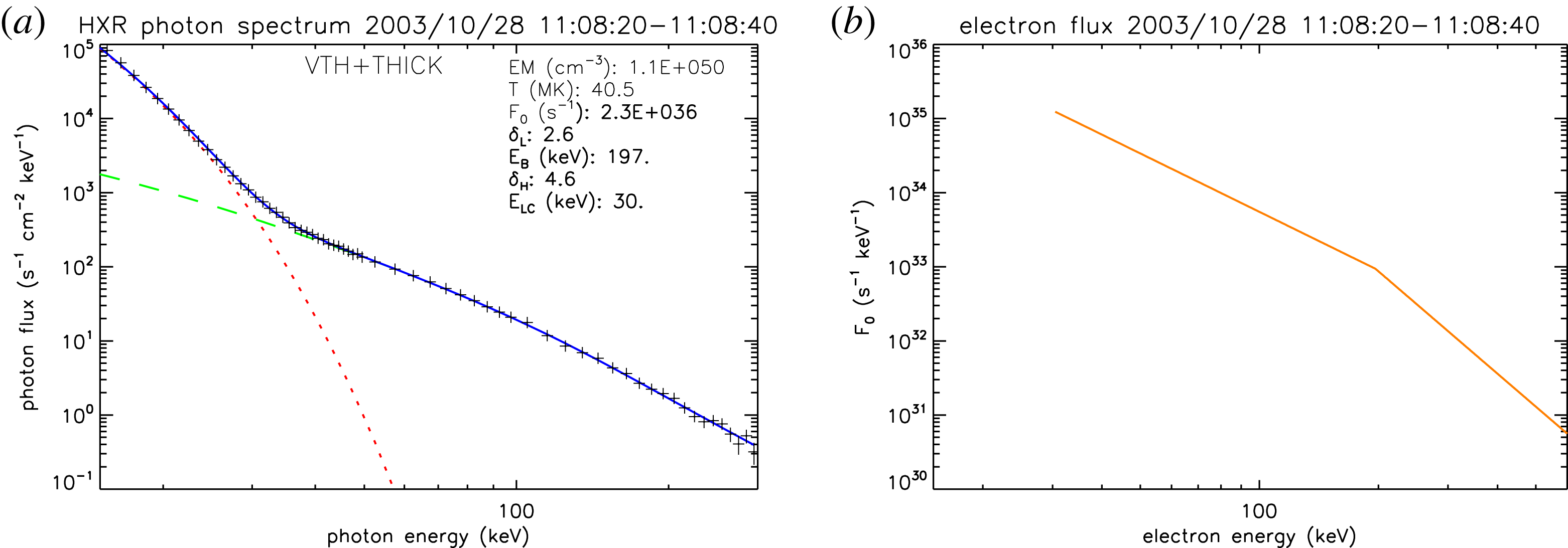
). The X-ray spectrum of figure 5 is a typical flare spectrum. It consists of a thermal and non-thermal component. The non-thermal one is strongly pronounced above 28 keV and extends beyond 300 keV. The thermal component corresponds to a temperature of
 $40.5\times 10^{6}~\text{K}$
. The photon spectrum can be converted into a differential injected electron flux by means of the forward-fitting method developed by Holman et al. (Reference Holman, Sui, Schwartz and Emslie2003), taking into account the photospheric albedo – see the detailed description of the method in Warmuth et al. (Reference Warmuth, Holman, Dennis, Mann, Aurass and Milligan2009a
) (see figure 5
b). Of course, the conversion of the photon spectrum into the differential injected electron flux can be influenced by a non-uniform ionization of the target, albedo, Langmuir waves, return current, etc. All these effects can lead to changes in the resulting differential injected electron fluxes – see the discussion in the reviews by Holman et al. (Reference Holman, Aschwanden, Aurass, Battaglia, Grigis, Kontar, Liu, Saint-Hilaire and Zharkova2011) and Kontar et al. (Reference Kontar, Brown, Emslie, Hajdas, Holman, Hurford, Kašparová, Mallik, Massone and McConnell2011). Note that the high-energy-resolution data from RHESSI have permitted the first reliable model-independent conversion of observed X-ray spectra into electron spectra (Massone et al.
Reference Massone, Piana, Conway and Eves2003; Piana et al.
Reference Piana, Massone, Kontar, Emslie, Brown and Schwartz2003). For the example under discussion, the conversion of the photon spectrum provides a total flux
 $F_{e}=1.6\times 10^{36}~\text{s}^{-1}$
for electrons with an energy
 ${>}28~\text{keV}$
. It is related to an energy flux
 $P_{e}=1.5\times 10^{22}~\text{W}$
(Warmuth, Mann & Aurass Reference Warmuth, Mann and Aurass2007). The ratio
 $P_{e}/F_{e}=59~\text{keV}$
is the mean value of the energy of the electrons with energies
 ${>}28~\text{keV}$
as produced during this special flare.
(a) The X-ray photon spectrum as recorded by RHESSI during the period 11:08:20–11:08:40 UT on 28 October 2003. (b) The differential electron flux derived from the photon spectrum in (a) by means of the forward-fitting method developed by Holman et al. (Reference Holman, Sui, Schwartz and Emslie2003).

In order to study this subject in more detail, a sample of nine X-class GOES flares was chosen to calculate the differential electron flux during peak periods of hard X-ray fluxes. This sample covers flares in the GOES class range X1.3–X17.2, i.e. they are large flares. The differential fluxes calculated from the photon spectra by means of the forward-fitting method (Holman et al. Reference Holman, Sui, Schwartz and Emslie2003) can be described in terms of a broken power law
 $$\begin{eqnarray}j_{(E)}=j_{B}\left(\frac{E}{E_{B}}\right)^{-{\it\delta}},\end{eqnarray}$$
with
 ${\it\delta}={\it\delta}_{L}$
for
 $E_{lc}\leqslant E\leqslant E_{B}$
and
 ${\it\delta}={\it\delta}_{H}$
for
 $E_{B}\leqslant E$
. Here,
 $E_{lc}$
is the so-called low-energy cut-off,
 $E_{B}$
is the energy where the power law breaks, and
 $j_{B}$
is the differential flux at
 $E=E_{B}$
. The logarithmic mean of all nine differential fluxes provides:
 $j_{B}=2.8\times 10^{14}~\text{cm}^{-2}~\text{s}^{-1}~\text{keV}^{-1}$
,
 $E_{lc}=28~\text{keV}$
,
 $E_{B}=148~\text{keV}$
,
 ${\it\delta}_{l}=4.3$
and
 ${\it\delta}_{H}=4.7$
. These values can be considered as typical ones for large flares. (For more details, see Warmuth et al. (Reference Warmuth, Mann and Aurass2009b
) and Mann & Warmuth (Reference Mann and Warmuth2011).) Inserting these values into (2.3), the flux
 $F_{XCF}$
of electrons with energies
 ${>}28~\text{keV}$
is found to be
 $3.1\times 10^{18}~\text{cm}^{-2}~\text{s}^{-1}$
. These electrons carry an energy flux
 $P_{XCF}=1.2\times 10^{20}~\text{keV}~\text{cm}^{-2}~\text{s}^{-1}$
. Then,
 $P_{e}/F_{e}=39~\text{keV}$
is the mean energy of the electrons accelerated up to an energy
 ${>}28~\text{keV}$
during large flares. Note once again that these results are found for X-class flares, which are the largest ones.
2.3. Plasma conditions in the flare region
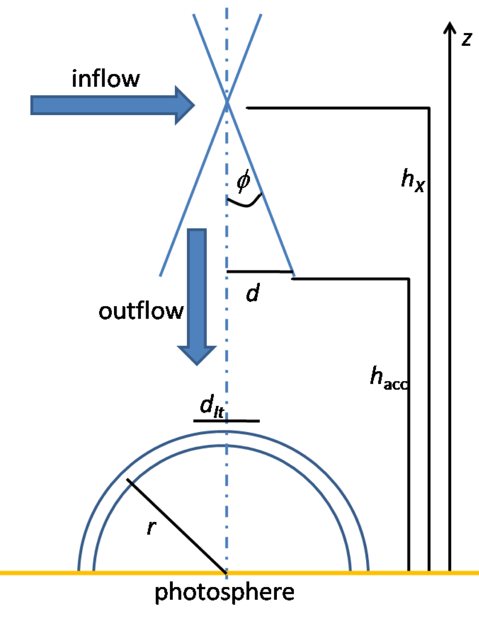
Figure 6 shows the geometry of the reconnection region in the corona according to the standard model (see figure 3). From solar radio data, i.e. pairs of forward and reversed drift bursts, the location of the X-point has already been found to be
 $h_{X}=60~\text{Mm}$
. Loops have typical radii of 10 Mm (Aschwanden Reference Aschwanden2002). The height
 $h_{acc}$
of the acceleration region is determined to be 20 Mm (Mann & Warmuth Reference Mann and Warmuth2011) by means of time-of-flight measurements by Burst and Transition Source Experiment (BATSE) onboard the Compton Gamma Ray Observatory (Aschwanden, Schwartz & Alt Reference Aschwanden, Schwartz and Alt1995b
; Aschwanden et al.
Reference Aschwanden, Kosugi, Hudson, Wills and Schwartz1996). Note that the location of the acceleration site is well below the location of the X-point and well above the loop top. Thus, the inflow region of all electrons, which finally travel towards the chromosphere, is typically located in the height range 20–60 Mm above the photosphere. At 40 Mm, an electron number density of
 $2.07\times 10^{9}~\text{cm}^{-3}$
(see (2.1)) and a magnetic field strength of 46 G (see (2.2)) as well as an Alfvén velocity of
 $2200~\text{km}~\text{s}^{-1}$
are obtained as typical plasma parameters in the inflow region (Mann & Warmuth Reference Mann and Warmuth2011). Note that these values should be considered as rough ones resulting from a statistical analysis of different flares. From RHESSI measurements, the flux of energetic electrons and the associated energy flux from the reconnection region are known. With this knowledge, Mann & Warmuth (Reference Mann and Warmuth2011) derived the conditions in the acceleration region by means of the conservation of the total electron number and energy. For large flares, the required huge flux (
 ${\approx}10^{36}~\text{s}^{-1}$
) of energetic electrons can only be delivered if the inflow speed is nearly equal to the high local Alfvén speed of
 ${\approx}2000{-}3000~\text{km}~\text{s}^{-1}$
. Recently, Wang, Sui & Qiu (Reference Wang, Sui and Qiu2007) reported on fast plasma flows with speeds of
 $900{-}3500~\text{km}~\text{s}^{-1}$
as signatures of magnetic reconnection in the corona. As a result, large flares can only occur in region with a high Alfvén speed.
Geometry of the reconnection region according to the standard model (see figure 3) (see figure 5 in Mann & Warmuth Reference Mann and Warmuth2011).

3. Electron acceleration mechanisms
NASA’s space mission RHESSI (Lin et al.
Reference Lin, Dennis, Hurford, Smith, Zehnder, Harvey, Curtis, Pankow, Turin and Bester2002) has the aim to study high-energy processes during solar flares. RHESSI observations require an answer to the question how such a large number of
 ${\approx}10^{36}$
electrons are accelerated up to energies
 ${>}30~\text{keV}$
within a fraction of a second during large flares. Since these electrons carry a substantial part of the flare released energy (Lin & Hudson Reference Lin and Hudson1971, Reference Lin and Hudson1976; Emslie et al.
Reference Emslie, Kucharek, Dennis, Gopalswamy, Holman, Share, Vourlidas, Forbes, Gallagher and Mason2004), the answer to this question plays an important role in the understanding of flares.
The reconnection region consists of the inflow, diffusion and outflow regions. The slow-mode shocks separate the inflow region from the outflow one (see figure 3). In the framework of the standard model, there are several ideas about where and in which way electrons can be accelerated (for reviews see Vrsnak Reference Vrsnak and Klein2003; Zharkova et al. Reference Zharkova, Arzner, Benz, Browning, Dauphin, Emslie, Fletcher, Kontar, Mann and Onofri2011):
-
(i) In the diffusion region, magnetic islands can occur in the current sheet. These islands contract and merge with each other. Hence, they can be the source of energetic electrons (Drake et al. Reference Drake, Swisdak, Che and Shay2006; Bárta et al. Reference Bárta, Büchner, Karlický and Skála2011). Furthermore, a large-scale DC electric field is induced within the diffusion region. Electrons can be directly accelerated in this electric field, as studied by Speiser (Reference Speiser1984), Speiser & Lyons (Reference Speiser and Lyons1984), Holman (Reference Holman1985), Benz (Reference Benz1987), Litvinenko & Somov (Reference Litvinenko and Somov1993) and Litvinenko (Reference Litvinenko, Ramaty and Mandzhavidze2000), for instance. This process can even explain the acceleration of an electron up to high energies, but it is not able to provide a high production rate of energetic electrons of typically
$10^{36}~\text{s}^{-1}$
as required by the observations because the diffusion region is spatially very small. -
(ii) In the outflow region, the newly reconnected magnetic field lines represent a collapsing magnetic trap in the corona. In such collapsing traps, electrons can be accelerated, as studied by Somov & Kosugi (Reference Somov and Kosugi1997), Karlický & Kosugi (Reference Karlický and Kosugi2004) and Grady & Neukirch (Reference Grady and Neukirch2009).
-
(iii) In both the diffusion and outflow regions, the plasma is highly turbulent. Thus, electrons can be accelerated by stochastic acceleration via wave–particle interaction there (Melrose Reference Melrose1994; Miller, Larosa & Moore Reference Miller, Larosa and Moore1996; Miteva & Mann Reference Miteva and Mann2007; Petrosian & Chen Reference Petrosian and Chen2010; Guo et al. Reference Guo, Emslie, Kontar, Benvenuto, Massone and Piana2012; Chen & Petrosian Reference Chen and Petrosian2013; Fleishman & Toptygin Reference Fleishman and Toptygin2013; Bian et al. Reference Bian, Emslie, Stackhouse and Kontar2014). The mechanism of stochastic electron acceleration can explain a lot of the observations related to hard X-ray emission during flares.
-
(iv) If the outflow jet becomes super-Alfvénic, a fast magnetosonic shock, usually called TS, is established due to the interaction of the jet with the surrounding coronal plasma. Signatures of such shocks are readily seen in the solar radio burst radiation (Aurass, Vršnak & Mann Reference Aurass, Vršnak and Mann2002; Aurass & Mann Reference Aurass and Mann2004). The spatial extension of these shocks is assumed to be roughly the width of the loop-top hard X-ray sources first observed by Masuda et al. (Reference Masuda, Kosugi, Hara, Tsuneta and Ogawara1994), i.e.
${\approx}7000~\text{km}$
(Tsuneta et al.
Reference Tsuneta, Masuda, Kosugi and Sato1997). The spatial extent of the TS is much greater than that of the diffusion region, and hence many more electrons can be accelerated at such shocks than in the diffusion region. Therefore, Tsuneta & Naito (Reference Tsuneta and Naito1998) proposed that this shock could be the source of energetic electrons. This mechanism was studied in a quantitative manner for the production of energetic electrons (i.e.
${>}30~\text{keV}$
) by Mann, Aurass & Warmuth (Reference Mann, Aurass and Warmuth2006) and Mann et al. (Reference Mann, Warmuth and Aurass2009). -
(v) In the standard model, the slow-mode shocks separate the inflow region from the outflow one. At these shocks, magnetic field energy inflowing towards the reconnection region is transformed into heating of the plasma in the downstream region (Tsuneta et al. Reference Tsuneta, Masuda, Kosugi and Sato1997). That happens efficiently in regions where the Alfvén velocity is extremely large in comparison to the sound speed (Cargill & Priest Reference Cargill and Priest1982). That is even the case in the solar corona. Thus, the heating of the plasma at the slow-mode shocks provides enough electrons with energies beyond 30 keV as required by RHESSI observations (Mann et al. Reference Mann, Aurass, Önel and Warmuth2014).


In § 3.1, the acceleration of electrons at the TS is presented in more detail. The role played by the slow-mode shocks for the production of energetic electrons is discussed in § 3.2.
3.1. Electron acceleration at the TS
It is well known that shocks are able to accelerate particles up to high energies in space. Hence, they are considered as the source of cosmic rays (Fermi Reference Fermi1949; Axford, Leer & Skadron Reference Axford, Leer, Skadron, Dergachev and Kocharov1978; Schlickeiser Reference Schlickeiser1984; Kirk Reference Kirk, Kirk, Melrose, Priest, Benz and Courvoisier1994). Therefore, Tsuneta & Naito (Reference Tsuneta and Naito1998) proposed that the TS in the outflow region is the source of energetic electrons needed for the generation of hard X-ray radiation during flares.
If the speed of the outflow plasma becomes super-Alfvénic, a shock wave is established. An obstacle such as, for example, an underlying loop is not necessary for that. If a super-Alfvénic flow (or jet) is penetrating into the surrounding plasma, it is decelerated owing to the jet–plasma interaction. The transition of a super-Alfvénic flow into a sub-Alfvénic one can basically happen only in terms of a shock wave (see e.g. Priest Reference Priest1982), which is a dissipative discontinuity. Hence, the TS is a fast-mode shock.
Such shocks are accompanied by a compression of both the density and the magnetic field (see e.g. Priest Reference Priest1982). Hence, they represent moving magnetic mirrors at which charged particles can be reflected and accelerated. The acceleration happens with the electric field induced in the shock transition region. This mechanism is usually called shock drift acceleration (Holman & Pesses Reference Holman and Pesses1983; Leroy & Mangeney Reference Leroy and Mangeney1984; Wu Reference Wu1984). In this section, we consider the TS to be the source of energetic electrons as originally proposed by Tsuneta & Naito (Reference Tsuneta and Naito1998). Since hard X-ray radiation with energies
 ${>}100~\text{keV}$
is emitted during flares (Lin & Hudson Reference Lin and Hudson1976), electrons with energies
 ${>}100~\text{keV}$
must be produced. Then, the shock drift acceleration of electrons at the TS must be treated in a fully relativistic manner as done by Mann et al. (Reference Mann, Aurass and Warmuth2006).
Following the approach by Ball & Melrose (Reference Ball and Melrose2001) and Mann & Klassen (Reference Mann and Klassen2005), the shock drift acceleration is treated in the de Hoffmann–Teller frame, which is defined by removing the motional electric field. Note that the shock is also at rest in this frame. Then, the reflection process can be described by taking into account the conservation of energy and magnetic moment of the particle. Note that all these transformations must necessarily be Lorentzian ones, in contrast to the non-relativistic approach. Doing that, relationships between the velocity components parallel
 $V_{\Vert }$
and perpendicular
 $V_{\bot }$
to the upstream magnetic field before (
 $i$
) and after (
 $r$
) the reflection are obtained:
 $$\begin{eqnarray}{\it\beta}_{r,\Vert }=\frac{2{\it\beta}_{s}-{\it\beta}_{i,\Vert }(1+{\it\beta}_{s}^{2})}{1-2{\it\beta}_{i,\Vert }{\it\beta}_{s}+{\it\beta}_{s}^{2}}\end{eqnarray}$$
and
 $$\begin{eqnarray}{\it\beta}_{r,\bot }=\frac{(1-{\it\beta}_{s}^{2})}{1-2{\it\beta}_{i,\Vert }{\it\beta}_{s}+{\it\beta}_{s}^{2}}{\it\beta}_{i,\bot },\end{eqnarray}$$
with
 ${\it\beta}_{\Vert }=V_{\Vert }/c$
and
 ${\it\beta}_{\bot }=V_{\bot }/c$
(Mann et al.
Reference Mann, Aurass and Warmuth2006), respectively. Here, if
 $v_{s}$
represents the shock speed in the laboratory frame, then
 ${\it\beta}_{s}=v_{s}\sec {\it\theta}_{1}/c$
denotes the shock speed in the de Hoffmann–Teller frame, i.e. the shock speed projected onto the magnetic field line, and
 ${\it\theta}_{1}$
is the angle between the shock normal and the upstream magnetic field. Note that here all velocities are normalized to the velocity of light
 $c$
.
Additionally, the reflection conditions
 $$\begin{eqnarray}{\it\beta}_{i,\Vert }\leqslant {\it\beta}_{s}\end{eqnarray}$$
and
 $$\begin{eqnarray}{\it\beta}_{i,\bot }\geqslant \frac{\tan {\it\alpha}_{lc}}{\sqrt{1-{\it\beta}_{s}^{2}}}({\it\beta}_{s}-{\it\beta}_{i,\Vert })\end{eqnarray}$$
must be fulfilled by the initial particles in order to be accelerated. The first one means that the shock must be able to touch a particle in the upstream region. The second one results from the conditions of conservation of the magnetic moment. The loss-cone angle
 ${\it\alpha}_{lc}$
is defined by
 ${\it\alpha}_{lc}=\arcsin \,[(B_{1}/B_{2})^{1/2}]$
with
 $B_{1}$
and
 $B_{2}$
as the magnetic field strength in the up- and downstream regions, respectively. Note that this treatment of the shock drift acceleration has been done independently on the charge and mass of the particle. Hence, the results are valid for both electrons and protons.
In the non-relativistic limit, i.e.
 ${\it\beta}_{\Vert },{\it\beta}_{\bot },{\it\beta}_{s}\ll 1$
, (3.1) and (3.2) reduce to
 $V_{r,\Vert }=2v_{s}\sec {\it\theta}_{1}-V_{i,\Vert }$
,
 $V_{r,\bot }=V_{i,\bot }$
and
 $V_{i\bot }\geqslant (v_{s}\sec {\it\theta}_{1}-V_{i,\Vert })\tan {\it\alpha}_{lc}$
(Holman & Pesses Reference Holman and Pesses1983; Ball & Melrose Reference Ball and Melrose2001; Mann & Klassen Reference Mann and Klassen2005). For example, assuming
 $10\times 10^{6}~\text{K}$
as a typical temperature in the flare region (Aschwanden Reference Aschwanden2005), the electrons have a thermal velocity of
 $12\,300~\text{km}~\text{s}^{-1}$
there. Radio observations reveal
 $1500~\text{km}~\text{s}^{-1}$
as a typical speed of the TS (Aurass et al.
Reference Aurass, Vršnak and Mann2002; Aurass & Mann Reference Aurass and Mann2004). Then, the velocity gain
 ${\rm\Delta}V=2v_{s}\sec {\it\theta}_{1}$
due to shock drift acceleration exceeds the one-, four- and 10-fold thermal speed for
 ${\it\theta}_{1}=75.9^{\circ }$
,
 $86.5^{\circ }$
and
 $88.6^{\circ }$
, respectively. That demonstrates that shock drift acceleration becomes very efficient if
 ${\it\theta}_{1}\rightarrow 90^{\circ }$
, i.e. in the case of nearly perpendicular shocks.
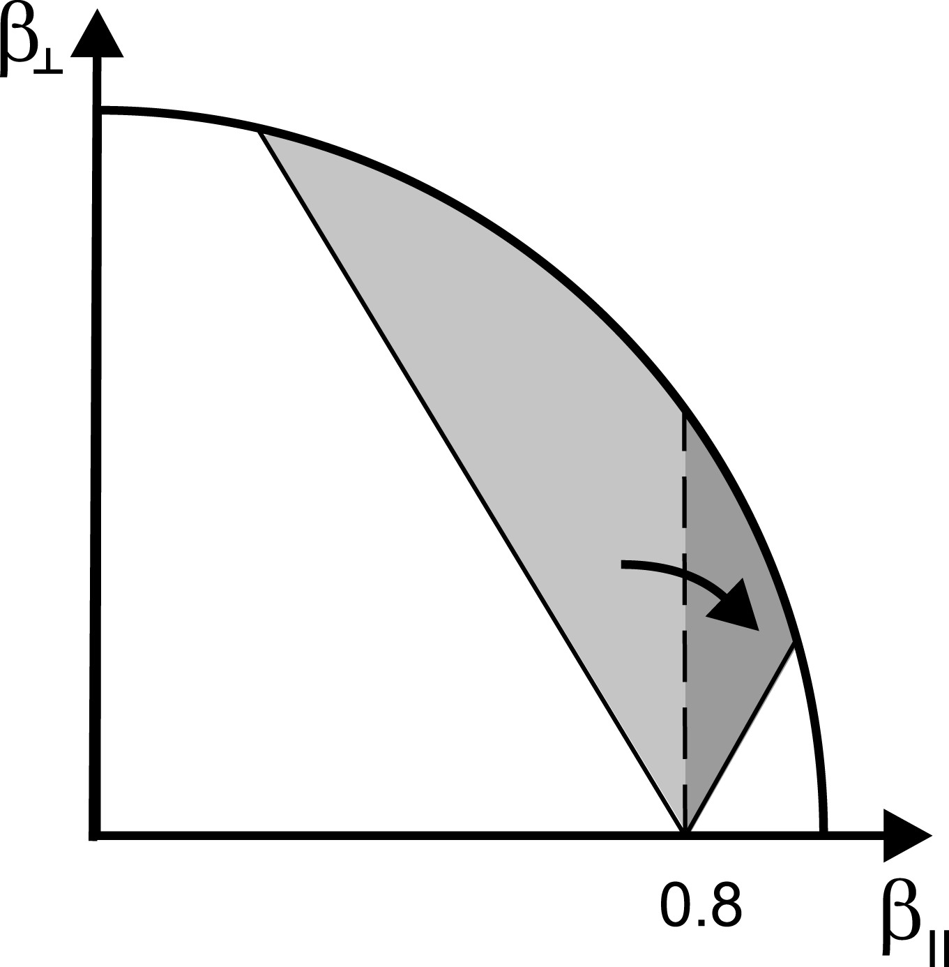
Illustration of the shock drift acceleration in the
 ${\it\beta}_{\bot }{-}{\it\beta}_{\Vert }$
plane for a shock wave with
 ${\it\beta}_{s}=0.8$
,
 $B_{2}/B_{1}=2$
and
 ${\it\alpha}_{lc}=45^{\circ }$
(see figure 2 in Mann et al.
Reference Mann, Warmuth and Aurass2009).

The shock drift acceleration actually represents a transformation in the
 ${\it\beta}_{\bot }{-}{\it\beta}_{\Vert }$
plane as illustrated in figure 7. The initial particles located in the grey area left of the dashed line are transformed into the dark one to the right of it due to shock drift acceleration, as indicated by the arrow in figure 7. This transformation leads to both a gain of energy of each individual particle and an enhancement of the particle number density at high energies in the phase space. That even means particle acceleration.
As seen in figure 7, the resulting distribution function of the accelerated electrons is a shifted loss-cone distribution as in the non-relativistic case (Leroy & Mangeney Reference Leroy and Mangeney1984; Wu Reference Wu1984). In the upstream region a Maxwellian distribution function is assumed for the initial state
 $$\begin{eqnarray}f_{M}({\it\beta}_{\Vert },{\it\beta}_{\bot })=C_{M}\text{e}^{-E_{kin}/k_{B}T}\end{eqnarray}$$
(
 $k_{B}$
is Boltzmann’s constant and
 $T$
is temperature), where the temperature
 $T_{1}$
in the upstream region has to be used in this case. Here, the kinetic energy
 $E_{kin}$
is defined by
 $$\begin{eqnarray}E_{kin}=m_{e}c^{2}\left[\frac{1}{\sqrt{1-{\it\beta}^{2}}}-1\right],\end{eqnarray}$$
with the electron mass
 $m_{e}$
and
 ${\it\beta}^{2}={\it\beta}_{\Vert }^{2}+{\it\beta}_{\bot }^{2}$
. Since all particles that fulfill the reflection conditions (see (3.3) and (3.4)) are finally accelerated, the distribution function of the reflected and accelerated particles is derived as
 $$\begin{eqnarray}\displaystyle f_{acc}=C_{M}{\it\Theta}({\it\beta}_{\Vert }-{\it\beta}_{s}){\it\Theta}({\it\beta}_{\bot }-D[{\it\beta}_{s}-{\it\beta}_{\Vert }])\exp \left[\frac{(-1)}{{\it\epsilon}_{th}}\left(\frac{1-2{\it\beta}_{s}{\it\beta}_{\Vert }+{\it\beta}_{s}^{2}}{(1-{\it\beta}_{s}^{2})(1-{\it\beta}^{2})^{1/2}}-1\right)\right],\hspace{-3.60004pt} & & \displaystyle \nonumber\\ \displaystyle & & \displaystyle\end{eqnarray}$$
with
 $D=\tan {\it\alpha}_{lc}/(1-{\it\beta}_{s}^{2})^{1/2}$
,
 ${\it\epsilon}_{th}=k_{B}T_{1}/m_{e}c^{2}$
and
 ${\it\epsilon}=E_{kin}/m_{e}c^{2}$
(Mann et al.
Reference Mann, Warmuth and Aurass2009).
As already mentioned in § 2.2 the hard X-ray spectra as measured with RHESSI, for instance, can be converted into a differential flux spectrum of energetic electrons emitting hard X-ray radiation. Hence, the differential flux of energetic electrons is the quantity that can link the theoretical results with the observations.
In a magnetized plasma, as in the corona, the electrons can only propagate along the magnetic field lines over long distances. Hence, they follow the magnetic field lines from the reconnection region in the corona to the dense chromosphere, where they can emit X-ray radiation by bremsstrahlung (Brown Reference Brown1971). Therefore, the magnetic field-aligned flux of electrons is the quantity of interest. It is generally defined by
 $$\begin{eqnarray}{\it\Phi}_{\Vert }=N\int \text{d}\boldsymbol{p}\boldsymbol{\cdot }\boldsymbol{V}_{\Vert }\,f.\end{eqnarray}$$
Note that the velocity distribution function is normalized to unity here, and
 $N$
denotes the particle number density. The particle velocity
 $\boldsymbol{V}={\bf\beta}\,c$
and its momentum
 $\boldsymbol{p}$
are related by
 $$\begin{eqnarray}\boldsymbol{p}=\frac{m_{e}c\,{\bf\beta}}{\sqrt{1-{\it\beta}^{2}}}\quad \text{and}\quad {\bf\beta}=\frac{\boldsymbol{p}^{\prime }}{\sqrt{1+p^{\prime 2}}}.\end{eqnarray}$$
With
 $p_{\Vert }^{\prime }$
and
 $p_{\bot }^{\prime }$
as the normalized momentum (
 $\boldsymbol{p}^{\prime }=\boldsymbol{p}/m_{e}c$
) parallel and perpendicular to the magnetic field, respectively, the magnetic field-aligned flux (see (3.8)) can be written as
 $$\begin{eqnarray}{\it\Phi}_{\Vert }=2{\rm\pi}Nc(m_{e}c)^{3}\int _{0}^{\infty }\,\text{d}p_{\Vert }^{\prime }\,\text{d}p_{\bot }^{\prime }\,p_{\bot }^{\prime }\frac{p_{\Vert }^{\prime }}{\sqrt{1+p^{\prime 2}}}f,\end{eqnarray}$$
with
 $p^{\prime }=(p_{\Vert }^{\prime 2}+p_{\bot }^{\prime 2})^{1/2}$
and/or
 $$\begin{eqnarray}{\it\Phi}_{\Vert }=2{\rm\pi}Nc(m_{e}c)^{3}\int _{0}^{1}\,\text{d}{\it\beta}_{\Vert }\,\text{d}{\it\beta}_{\bot }\,\frac{{\it\beta}_{\Vert }{\it\beta}_{\bot }}{(1-{\it\beta}^{2})^{5/2}}f.\end{eqnarray}$$
In the case of an isotropic distribution function, as for a Maxwellian one, for example, the integral in (3.11) can be treated by means of polar coordinates (
 $p_{\Vert }^{\prime }=p^{\prime }\cos {\it\alpha}$
and
 $p_{\bot }^{\prime }=p^{\prime }\sin {\it\alpha}$
) with pitch angle
 ${\it\alpha}$
. The integration with respect to pitch angle
 ${\it\alpha}$
must be performed from 0 to
 ${\rm\pi}/2$
. As a result, one gets an expression for the magnetic field-aligned flux of electrons in terms of an integral with respect to
 ${\it\epsilon}$
:
 $$\begin{eqnarray}{\it\Phi}_{\Vert }={\rm\pi}Nc(m_{e}c)^{3}\int _{0}^{\infty }\,\text{d}{\it\epsilon}\,{\it\epsilon}(2+{\it\epsilon})f.\end{eqnarray}$$
The differential flux is generally defined by
 $$\begin{eqnarray}j_{\Vert }(E_{kin})=\frac{\text{d}{\it\Phi}_{\Vert }}{\text{d}E_{kin}}=\frac{\text{d}{\it\epsilon}}{\text{d}E_{kin}}\,\frac{\text{d}{\it\Phi}_{\Vert }}{\text{d}{\it\epsilon}}=\frac{1}{m_{e}c^{2}}\,\frac{\text{d}{\it\Phi}_{\Vert }}{\text{d}{\it\epsilon}}.\end{eqnarray}$$
For an example, in the case of a Maxwell distribution (see (3.5)), the normalization constant
 $C_{M}$
is determined to be
 $$\begin{eqnarray}\frac{1}{C_{M}}=4{\rm\pi}(m_{e}c)^{3}\int _{0}^{\infty }\,\text{d}{\it\epsilon}\,\sqrt{{\it\epsilon}(2+{\it\epsilon})}\,(1+{\it\epsilon})\text{e}^{-{\it\epsilon}/{\it\epsilon}_{th}}.\end{eqnarray}$$
Then, the differential flux of a pure Maxwellian distribution can be derived to be
 $$\begin{eqnarray}j_{\Vert }=\frac{Nc}{m_{e}c^{2}}{\rm\pi}C_{M}{\it\epsilon}(2+{\it\epsilon})\text{e}^{-{\it\epsilon}/{\it\epsilon}_{th}}\end{eqnarray}$$
from (3.5), (3.12) and (3.14).
The differential flux of the electrons accelerated by shock drift acceleration can be calculated by inserting the distribution function (3.7) into (3.11) and subsequently performing the integration with respect to
 ${\it\beta}_{\Vert }$
and
 ${\it\beta}_{\bot }$
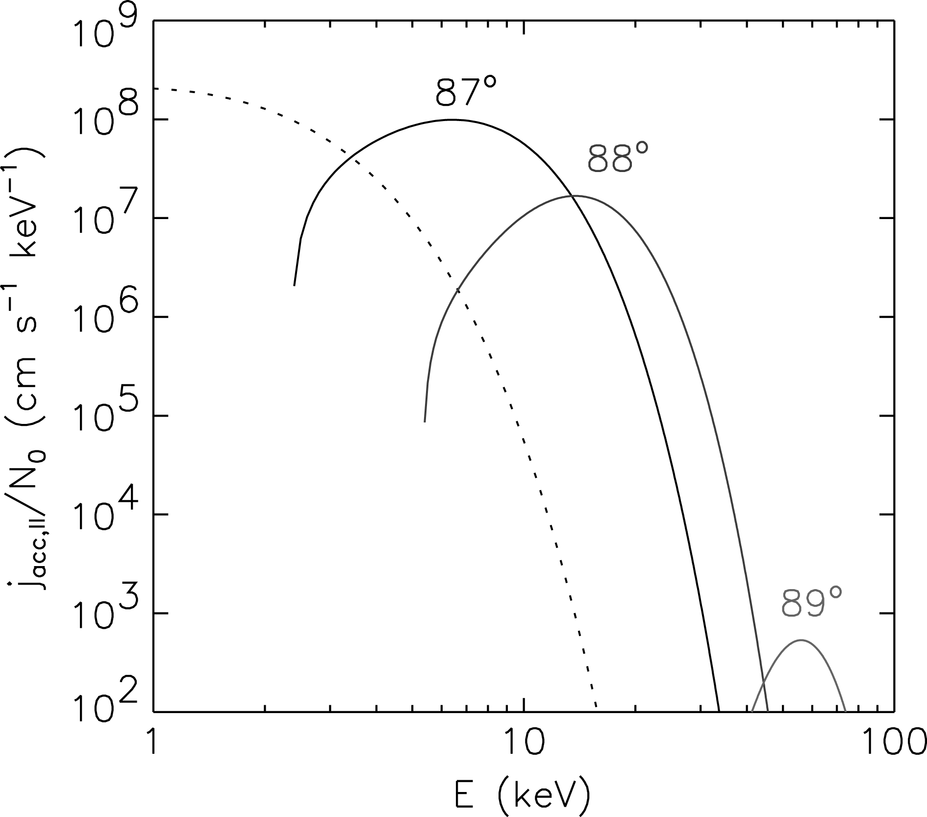
. That was done by Mann et al. (Reference Mann, Warmuth and Aurass2009). In figure 8, these fluxes are shown for several angles
 ${\it\theta}$
using typical parameters of the TS, i.e. a shock speed
 $v_{s}=1500~\text{km}~\text{s}^{-1}$
(Aurass et al.
Reference Aurass, Vršnak and Mann2002; Aurass & Mann Reference Aurass and Mann2004) and a temperature
 $T_{1}=10\times 10^{6}~\text{K}$
in the flare (Aschwanden Reference Aschwanden2005). For comparison, the flux of a pure Maxwellian distribution of the same temperature is also presented in figure 8. Figure 8 demonstrates that the fluxes of the accelerated electrons greatly exceed that of a pure Maxwellian population at high energies. The differential fluxes of the accelerated electrons have a local maximum, which shifts towards higher energies with increasing angle
 ${\it\theta}_{1}$
. But the flux at the maximum decreases strongly with increasing angle
 ${\it\theta}_{1}$
. Those are typical properties of shock drift acceleration.
The differential magnetic field-aligned flux for electrons accelerated by shock drift acceleration for several angles
 ${\it\theta}_{1}$
. Here
 $N_{0}$
is the electron number density; the shock speed is
 $1500~\text{km}~\text{s}^{-1}$
; and the loss-cone angle is
 $45^{\circ }$
according to the jump of the magnetic field
 $B_{2}/B_{1}=2$
across the shock. For comparison, the corresponding flux of a pure Maxwellian population is presented by the dashed line. A temperature
 $10\times 10^{6}~\text{K}$
is adopted in the upstream region (see figure 3 in Mann et al.
Reference Mann, Warmuth and Aurass2009).

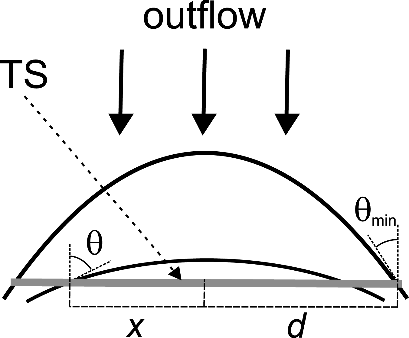
Magnetic field geometry at the TS. The reconnected magnetic field lines are pushed across the TS. It takes an angle
 ${\it\theta}$
with the shock normal at the point
 $x$
(see figure 4 in Mann et al.
Reference Mann, Warmuth and Aurass2009).

In figure 8, a Maxwellian distribution has been assumed as the initial one in the upstream region. However, in space plasmas, electron distribution functions are not usually Maxwellian but show an enhanced super-thermal tail (Lin et al. Reference Lin, Larson, McFadden, Carlson, Ergun, Anderson, Ashford, McCarthy, Parks and Rème1996). They are usually described by kappa distributions
 $$\begin{eqnarray}f_{{\it\kappa}}=C_{{\it\kappa}}\left[1+\frac{E_{kin}}{{\it\kappa}E_{{\it\kappa}}}\right]^{-({\it\kappa}+1)}\end{eqnarray}$$
(see Maksimovic, Pierrard & Riley Reference Maksimovic, Pierrard and Riley1997; Pierrard, Maksimovic & Lemaire Reference Pierrard, Maksimovic and Lemaire1999). The case in which a kappa distribution is the initial one in the upstream region is discussed in detail by Mann et al. (Reference Mann, Warmuth and Aurass2009).
The efficiency of shock drift acceleration is crucially dependent on the angle
 ${\it\theta}$
, as figure 8 shows. The magnetic field geometry at the TS is sketched in figure 9. The magnetic field lines are reconnected in the diffusion region (see figure 3) and subsequently convected into the outflow region across the TS. Owing to the curvature of the magnetic field line at the TS, the angle
 ${\it\theta}_{1}$
between the magnetic field and the shock normal varies locally across the shock. Since the shock speed in the de Hoffmann–Teller frame may not exceed the velocity of light, the value of the angle
 ${\it\theta}_{1}$
is limited by
 ${\it\theta}_{1}<\arccos \,(v_{s}/c)$
, i.e.
 ${\it\theta}_{1}<89.7^{\circ }$
for
 $v_{s}=1500~\text{km}~\text{s}^{-1}$
. Hence, electrons with different energies are generated at different places at the TS, resulting in a broad spectrum of energetic electrons, as observed.
At shock drift acceleration, the particles are reflected at the shock by the mirror force and accelerated by the electric field induced in the shock transition region. Basically, the accelerated particles propagate along the magnetic field lines in the upstream region. Owing to the curvature of the magnetic field lines upstream of the TS (see figure 9), they will encounter the shock once again. Since the pitch angle decreases significantly at the first encounter (see (3.2)), the reflection conditions (see (3.4)) are not fulfilled by most of them, so that they can transmit into the downstream region, where they travel along the magnetic field lines towards the chromosphere. There, they emit hard X-rays via bremsstrahlung (Brown Reference Brown1971).
Warmuth et al. (Reference Warmuth, Mann and Aurass2009b
) discussed whether shock drift acceleration at the TS is able to produce the energetic electrons needed for the hard X-ray emission during flares. For that, the theoretically obtained spectra are compared with the electron spectra derived from hard X-ray spectra measured with RHESSI. Shock drift acceleration can reproduce the total particle and energy fluxes of the electrons with energies beyond the low-energy cut-off, if the plasma in the outflow region is significantly heated and the area of the TS is sufficiently large. The theoretically obtained spectra do not show a true power-law behaviour, but the energy-dependent spectra indices are in the right range (i.e. 3–5) up to
 ${\approx}100~\text{keV}$
. However, shock drift acceleration at the TS is able to reproduce the spectral evolution of hard X-ray flare radiation, i.e. the relation between flux and spectral indices: the observed soft–hard–soft and soft–hard–harder evolutions of the hard X-ray spectra (Kiplinger Reference Kiplinger1995; Grigis & Benz Reference Grigis and Benz2004). The observed sub-second hard X-ray bursts can be explained by a variation of the angle
 ${\it\theta}_{1}$
in the framework of this model.
3.2. Energization of electrons at the slow-mode shocks in the reconnection region
In contradiction to the fast-mode shocks, at which the kinetic energy of the inflow in the upstream region is transferred to heating of the plasma in the downstream region, at the slow-mode shocks, the inflowing magnetic field energy is transformed to heating of the downstream plasma. Thus, the following question arises. What role does the slow-mode shocks play for the energization of electrons in the reconnection region? That is the subject of this subsection (see Mann et al. (Reference Mann, Aurass, Önel and Warmuth2014)).
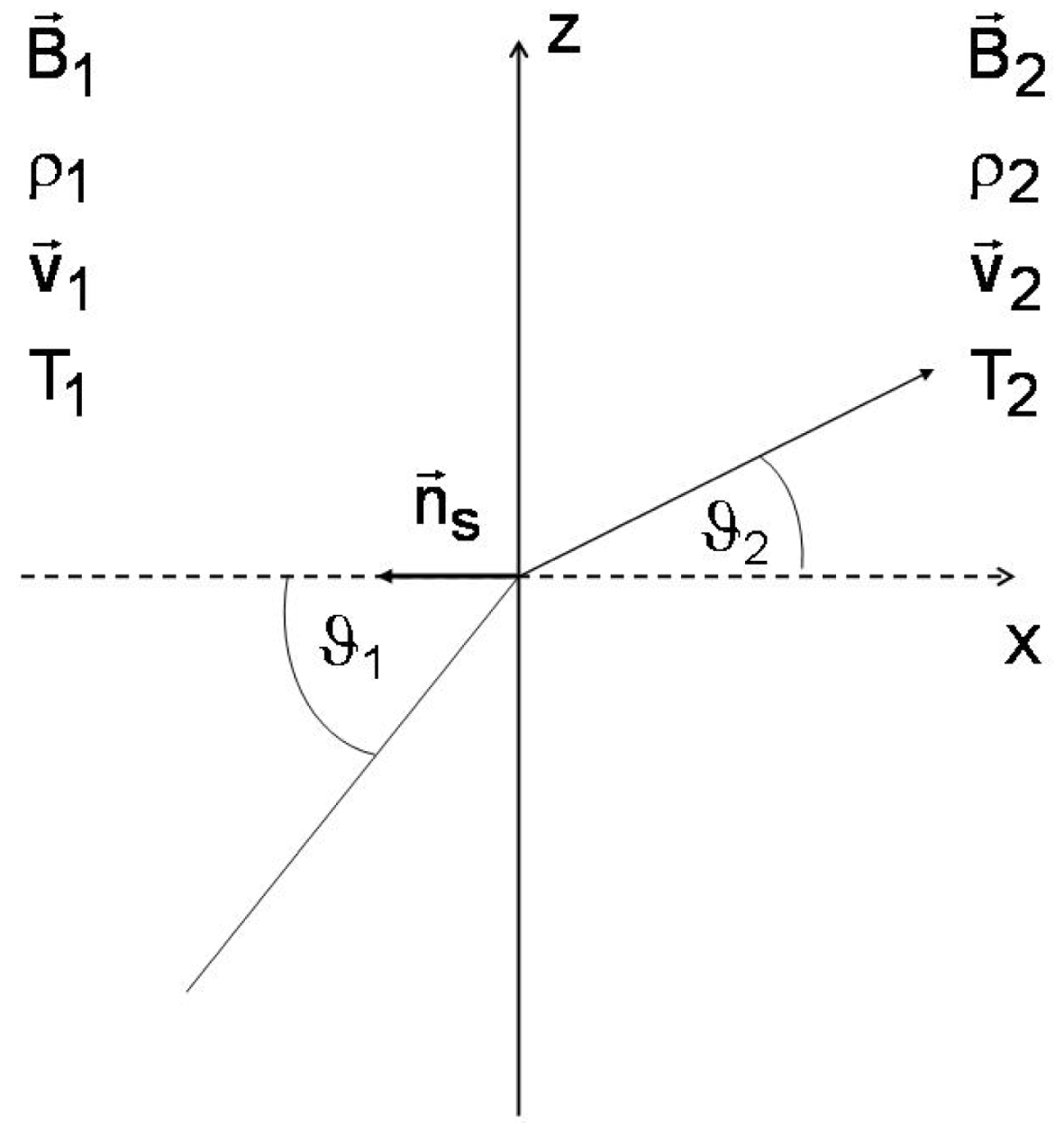
The framework of the shock is given in figure 10. The shock normal
 $\boldsymbol{n}_{s}$
is directed along the
 $x$
axis, i.e. the shock itself is located in the
 $y{-}z$
plane. The magnetic field
 $\boldsymbol{B}$
is in the
 $x{-}z$
plane and takes an angle
 ${\it\theta}_{1}$
to the
 $x$
axis in the upstream region. As previously, all quantities with subscripts 1 and 2 denote those in the up- and downstream region, respectively.
Since the slow-mode shocks separate the in- and outflow regions, the in- and outflow regions are the up- and downstream ones with respect to the shock transition, respectively. Basically, a shock is a dissipative structure at which quantities such as density, magnetic field and temperature jump, i.e. it is a discontinuity. In the framework of magnetohydrodynamics (MHD), shocks are described by the requirement of the conservation of mass, momentum, energy and magnetic flux across the shock (Priest Reference Priest1982). These jumps can be expressed in terms of the compression ratio
 $X={\it\rho}_{2}/{\it\rho}_{1}$
. They are supplemented by a polynomial of the third order in
 $X$
. Here, the mass density
 ${\it\rho}$
is related to the full particle number density
 $N$
by
 ${\it\rho}=\tilde{{\it\mu}}m_{p}N$
(
 $m_{p}$
is the proton mass and
 $\tilde{{\it\mu}}$
is the mean molecular weight). Additionally, the equation of state
 $p=Nk_{B}T$
(
 $p$
is pressure,
 $T$
is temperature and
 $k_{B}$
is Boltzmann’s constant) has been used. All these equations are called Rankine–Hugoniot relationships. The jump of the magnetic field is found to be
 $$\begin{eqnarray}\frac{B_{1}^{2}-B_{2}^{2}}{B_{1}^{2}}=\frac{\mathit{Ma}_{A}^{2}}{(\mathit{Ma}_{A}^{2}-X)}(1-X)\sin ^{2}{\it\theta}_{1},\end{eqnarray}$$
with the Alfvén–Mach number
 $\mathit{Ma}_{A}=(v_{s}/v_{A1})\sec {\it\theta}_{1}$
. It is actually the Alfvén–Mach number in the de Hoffmann–Teller frame, where the motional electric field is removed. Here,
 $v_{s}$
denotes the shock speed in the laboratory frame. The Alfvén and sound velocities are defined by
 $v_{A1}=B_{1}/(4{\rm\pi}{\it\rho}_{1})^{1/2}$
and
 $c_{s1}=({\it\gamma}p_{1}/{\it\rho}_{1})^{1/2}$
respectively (where
 ${\it\gamma}$
is the ratio of the specific heats) in the upstream region.
The framework of the shock transition. The quantities
 $\boldsymbol{B}$
,
 ${\it\rho}$
,
 $\boldsymbol{v}$
and
 $T$
denote the magnetic field vector, the mass density, the vector of the flow velocity and the temperature in the up- (subscript 1) and downstream (subscript 2) regions, respectively; and
 $\boldsymbol{n}_{s}$
is the shock normal (see figure 2 in Mann et al. (Reference Mann, Aurass, Önel and Warmuth2014)).

The entropy must increase across the shock, leading to the requirement
 $X>1$
. Then, one gets
 $\mathit{Ma}_{A}\leqslant 1<X$
and
 $B_{1}>B_{2}$
for the slow-mode shocks. Thus, magnetic field energy is annihilated at the slow-mode shocks and transferred to the heating of the downstream plasma. According to the Rankine–Hugoniot relationships,
 $T_{2}/T_{1}\propto v_{A1}^{2}/c_{s1}^{2}$
is found for the temperature jump across the shock (Priest Reference Priest1982). Thus, the plasma of the downstream region is strongly heated in regions where the Alfvén speed is extremely high in comparison to the sound speed. That is even the case in flare regions (Mann & Warmuth Reference Mann and Warmuth2011) (see § 2). That can be explained in the following manner. Because
 $v_{A1}^{2}\propto B_{1}^{2}/N_{1}$
, there is a large amount of magnetic field energy available per particle in regions with a high Alfvén speed. Since, at the slow-mode shocks, magnetic field energy is transformed into kinetic energy (i.e. heating), that is most efficient in regions where enough magnetic field energy is available per particle, or in other words where the Alfvén velocity is high.
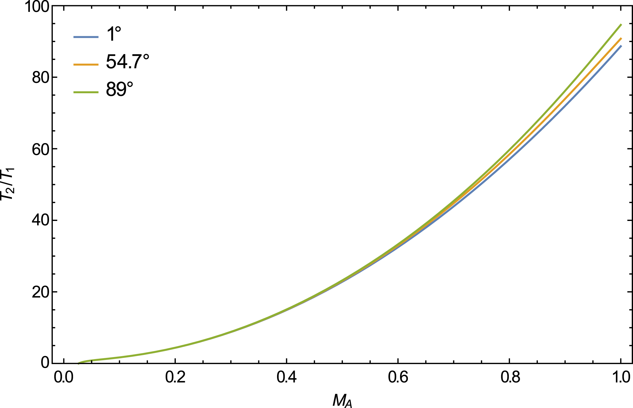
Figure 11 shows the dependence of
 $T_{2}/T_{1}$
on the Alfvén–Mach number
 $\mathit{Ma}_{A}$
for several angles
 ${\it\vartheta}_{1}$
. It can be seen that
 $T_{2}/T_{1}$
is only weakly dependent on
 ${\it\theta}_{1}$
. Inspection of figure 11 reveals that the downstream plasma is strongly heated if
 $\mathit{Ma}_{A}$
approaches 1 and hence
 $v_{s}=v_{A1}\cos {\it\theta}_{1}$
,
 $B_{2z}=0$
and
 ${\it\theta}_{2}=0$
. This special case is called a switch-off shock. For this case, the jump in the temperature is given by
 $$\begin{eqnarray}\frac{T_{2}}{T_{1}}=1+\frac{({\it\gamma}-1)}{2}\frac{v_{A1}^{2}}{c_{s1}^{2}}\left(1-\frac{\cos ^{2}{\it\theta}_{1}}{X^{2}}\right).\end{eqnarray}$$
Mann et al. (Reference Mann, Aurass, Önel and Warmuth2014) have shown that the transformation of the inflowing magnetic field energy to heating of the downstream plasma is most efficient for
 $\mathit{Ma}_{A}=1$
(i.e. for the switch-off shock) and
 ${\it\vartheta}_{1}=54.7^{\circ }$
. Then, the jump of the density is found to be
 ${\it\rho}_{2}/{\it\rho}_{1}=X=2.87$
by means of the numerical evaluation of the Rankine–Hugoniot relationships.
Dependence of the temperature jump
 $T_{2}/T_{1}$
across the slow-mode shock on the Alfvén–Mach number
 $\mathit{Ma}_{A}$
for
 ${\it\vartheta}_{1}=1^{\circ }$
,
 $54^{\circ }$
and
 $89^{\circ }$
with
 $v_{A1}=3000~\text{km}~\text{s}^{-1}$
. The sound speed
 $c_{s1}=179~\text{km}~\text{s}^{-1}$
is a typical one in the solar corona for
 $T_{1}=1.4\times 10^{6}~\text{K}$
and
 ${\it\gamma}=5/3$
.

As a result, at slow-mode shocks, magnetic field energy is efficiently annihilated and hence the downstream plasma is strongly energized (Cargill & Priest Reference Cargill and Priest1982; Somov & Syrovatskii Reference Somov and Syrovatskii1982; Forbes & Malherbe Reference Forbes and Malherbe1991).
Now we will discuss what consequences the slow-mode shocks have for producing energetic electrons during flares (see Mann et al. (Reference Mann, Aurass, Önel and Warmuth2014)). As already mentioned, the electron flux (see (3.8)) parallel to the magnetic field lines is the quantity of interest for comparing the theoretical results with observations. Now, a Maxwellian distribution (see (3.5)) is assumed in the downstream region, where the downstream temperature
 $T_{2}$
has to be used for the temperature in (3.5)). Then, one gets for the differential flux of electrons along the magnetic field lines (see (3.18))
 $$\begin{eqnarray}j_{\Vert }=\frac{\text{d}{\it\Phi}_{\Vert }}{\text{d}E}=j_{0}{\it\epsilon}(2+{\it\epsilon})\text{e}^{-{\it\epsilon}/{\it\epsilon}_{th}},\end{eqnarray}$$
with
 $j_{0}=(Nc/m_{e}c^{2}){\rm\pi}C_{M}(m_{e}c)^{3}$
. It has a local maximum at
 ${\it\epsilon}_{max}={\it\epsilon}_{th}-1+[1+{\it\epsilon}_{th}^{2}]^{1/2}$
. The maximum shifts towards higher energies for increasing temperatures. For example, it is 0.12 and 3.46 keV for a temperature of
 $1.4\times 10^{6}$
and
 $40\times 10^{6}~\text{K}$
, respectively. By means of (3.19), the flux of electrons with energies
 ${>}E_{lc}$
and the related energy flux can be calculated as
 $$\begin{eqnarray}\displaystyle F_{e} & = & \displaystyle (m_{e}c^{2})\int _{{\it\epsilon}_{lc}}^{\infty }\text{d}{\it\epsilon}\,j_{\Vert }\nonumber\\ \displaystyle & = & \displaystyle j_{0}m_{e}c^{2}\text{e}^{-w}[2{\it\epsilon}_{th}^{2}(1+w)+{\it\epsilon}_{th}^{3}(2+2w+w^{2})]\end{eqnarray}$$
and
 $$\begin{eqnarray}\displaystyle P_{e} & = & \displaystyle (m_{e}c^{2})^{2}\int _{{\it\epsilon}_{lc}}^{\infty }\text{d}{\it\epsilon}\,j_{\Vert }{\it\epsilon}\nonumber\\ \displaystyle & = & \displaystyle j_{0}(m_{e}c^{2})^{2}\text{e}^{-w}[2{\it\epsilon}_{th}^{3}(2+2w+w^{2})+{\it\epsilon}_{th}^{4}(3+6w+6w^{2}+w^{3})],\end{eqnarray}$$
with
 ${\it\epsilon}_{lc}=E_{lc}/m_{e}c^{2}$
and
 $w={\it\epsilon}_{lc}/{\it\epsilon}_{th}$
, respectively. In the limit
 ${\it\epsilon}_{th}\ll 1$
, (3.20) and (3.21) provide
 $$\begin{eqnarray}\frac{P_{e}}{F_{e}}=(m_{e}c^{2}){\it\epsilon}_{th}\frac{(2+2w+w^{2})}{(1+w)}.\end{eqnarray}$$
In order to compare these theoretical results with observations, GOES X-class flares are considered (see § 2.2). This seems to be appropriate since they are the largest ones and the strongest heating of the downstream plasma occurs at the switch-off slow-mode shocks. For these flares, the flux
 $F_{XCF}$
of electrons with energies
 ${>}28~\text{keV}$
and associated energy flux
 $P_{XCF}$
are
 $F_{XCF}=3.1\times 10^{18}~\text{cm}^{-2}~\text{s}^{-1}$
and
 $P_{e}=P_{XCF}=1.2\times 10^{20}~\text{keV}~\text{cm}^{-2}~\text{s}^{-1}$
(see § 2.2). If
 $F_{e}$
and
 $P_{e}$
are identified with
 $F_{XCF}$
and
 $P_{XCF}$
, respectively, inspection of (3.20) and (3.21) provides
 ${\it\epsilon}_{th}=0.0187$
corresponding to a temperature
 $T_{2}=1.11\times 10^{8}~\text{K}$
and
 $N_{2}=8.877\times 10^{9}~\text{cm}^{-3}$
. Note that they are the values of the temperature and the particle number density in the downstream plasma. Here,
 ${\it\epsilon}_{lc}=0.0547$
has been used because
 $E_{lc}=28~\text{keV}$
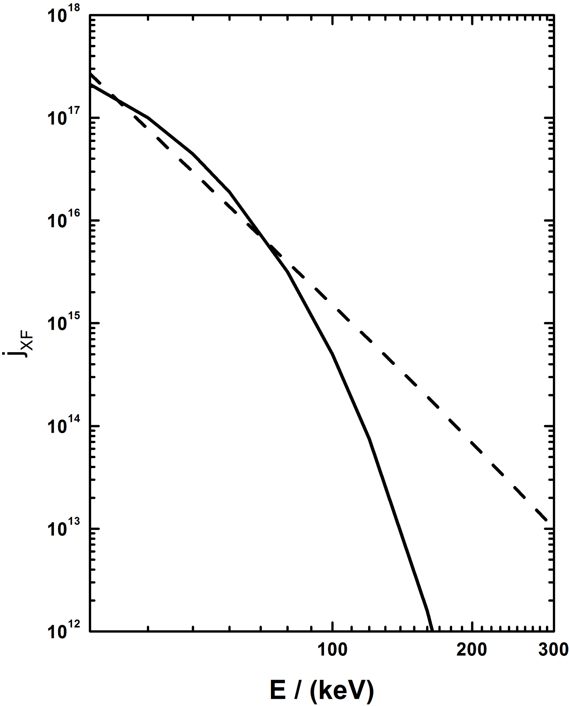
. In figure 12, the theoretically obtained differential electron flux (see (3.20)) for these values is compared with the measured one (see (2.3)). It shows that the theoretically obtained flux agrees well with the observed ones in the energy range 30–100 keV. Beyond 100 keV, the theoretical flux decreases faster than the observed ones, because it does not show a power-law behaviour. The reason for that is that a pure Maxwellian distribution is assumed for the downstream heated electrons. It may be that the electrons show basically a kappa distribution (Lin et al.
Reference Lin, Larson, McFadden, Carlson, Ergun, Anderson, Ashford, McCarthy, Parks and Rème1996; Maksimovic et al.
Reference Maksimovic, Pierrard and Riley1997; Pierrard et al.
Reference Pierrard, Maksimovic and Lemaire1999) in collisionless plasmas as in the solar corona. Then, a power-law behaviour would result from the heating at the slow-mode shocks. Nevertheless, the energization of electrons at the slow-mode shocks can well reproduce the observed particle fluxes and the associated energy fluxes of flare-generated electrons with energies beyond 30 keV. Therefore, the energization at the slow-mode shocks could be a potential mechanism for generating the energetic electrons needed for the hard X-ray radiation during flares.

Now, the plasma parameters in the upstream (or inflow) region can be deduced. Then,
 $N_{1}=N_{2}/X=8.877\times 10^{9}~\text{cm}^{-3}$
(because
 $X=2.87$
) is the particle number density in the upstream region. For the switch-off shock, (3.18) reduces to
 $T_{2}/T_{1}=1+0.32(v_{A1}^{2}/c_{s1}^{2})$
. Here,
 $X=2.87$
,
 ${\it\theta}_{1}=54.7^{\circ }$
and
 ${\it\gamma}=5/3$
have been used. Then, one gets
 $v_{A1}=2800~\text{km}~\text{s}^{-1}$
for the Alfvén velocity in the upstream plasma. Here, a typical coronal temperature
 $T_{1}=1.4\times 10^{6}~\text{K}$
provides a sound speed
 $c_{s1}=179~\text{km}~\text{s}^{-1}$
. This value of the Alfvén speed leads to a magnetic field strength
 $B_{1}=27~\text{G}$
in the upstream region. This is a typical value for the magnetic field above active regions in the corona (Dulk & McLean Reference Dulk and McLean1978). As a result,
 $8.9\times 10^{9}~\text{cm}^{-3}$
,
 $1.4\times 10^{6}~\text{K}$
and 27 G are typical values for the electron number density, temperature and magnetic field strength in regions where large flares can occur. These are coronal regions with large Alfvén velocities of about
 $2800~\text{km}~\text{s}^{-1}$
.
Adopting these values, 15 % of the electrons inflowing towards the reconnection region are accelerated up to energies beyond 28 keV at the slow-mode shocks. They carry 32 % of the flare-released energy. That agrees well with RHESSI observations (Oka et al. Reference Oka, Ishikawa, Saint-Hilaire, Krucker and Lin2013; Krucker & Battaglia Reference Krucker and Battaglia2014), namely that a substantial part of the flare-released energy is transferred to the energetic electrons. As a result, the energization of electrons at the slow-mode shocks in the magnetic reconnection region provides enough electrons with energies beyond 28 keV as needed for the observed hard X-ray flare emission.
4. Summary
Observations of the hard X-ray emission during flares, as done by NASA’s RHESSI spacecraft mission, reveal that a substantial part of the electrons are accelerated up to high energies (i.e. beyond 30 keV). The spectrum of these electrons can be described in terms of a power law (see § 2). The energetic electrons carry a substantial part of the flare-released energy. For this reason, the study of electron acceleration plays an important role in understanding flares. The study of the hard X-ray emission of large (i.e. GOES X-class) flares reveals that large flares occur in regions where the local Alfvén velocity is high, i.e. it must be beyond
 ${\approx}2500~\text{km}~\text{s}^{-1}$
.
Presently, flares are understood in the framework of the standard model (see § 1), in which a flare is considered as a manifestation of magnetic reconnection in the solar corona. Several mechanisms of electron acceleration (see § 3) have been proposed. They act at different places in the reconnection region, e.g. in the diffusion region, in the turbulent outflow region and at the TS as well as at the slow-mode shocks. The roles that both shocks play for generation of energetic electrons are discussed in detail in §§ 3.1 and 3.2. It was shown that shock drift acceleration at the TS provides enough energetic electrons as needed for the hard X-ray radiation if the outflow plasma in the upstream region of the TS is already sufficiently preheated. In the case of the slow-mode shocks, they generate enough energetic electrons if the Alfvén velocity in the inflow region of the reconnection site is high, i.e.
 ${>}2800~\text{km}~\text{s}^{-1}$
. Then,
 ${\approx}15\,\%$
of the inflowing electrons are accelerated up to energies
 ${>}30~\text{keV}$
and they carry
 ${\approx}35\,\%$
of the flare-released energy. These results are in good agreement with the observations. But the spectrum of these electrons does not show a power-law behaviour. The reason for that is that a Maxwellian distribution with an exponential decay is assumed for the electrons in the initial state, i.e. before the acceleration process. As already mentioned, so-called kappa distributions with a power-law decay in the supra-thermal tail are usually found for electrons in space plasmas. Adopting such a distribution as the initial one, then a power-law spectrum can result for the energetic electrons from shock drift acceleration at the TS. But, it is also possible that the electrons energized at the slow-mode shocks enter into the outflow region, where they are accelerated subsequently at the TS. Thus, electrons with very high energies can be produced.
Of course, stochastic acceleration of electrons is presently suggested to be the ‘best’ one to describe the observations of hard X-ray emission during flares (Petrosian & Chen Reference Petrosian and Chen2010; Guo et al.
Reference Guo, Emslie, Kontar, Benvenuto, Massone and Piana2012; Chen & Petrosian Reference Chen and Petrosian2013; Fleishman & Toptygin Reference Fleishman and Toptygin2013). Recently, Bian et al. (Reference Bian, Emslie, Stackhouse and Kontar2014) reported on a mechanism for the formation of a kappa distribution of flare-accelerated electrons. Owing to diffusive acceleration and Coulomb collisions in the flare region, the resulting electron distribution function approaches asymptotically towards a kappa distribution during its temporal evolution. As already emphasized, RHESSI observations vigorously support the standard (or CSHKP) model. According to this model, there are several sites (e.g. diffusion region, slow- and fast-mode shocks, highly turbulent outflow region) in the reconnection region where electrons can be accelerated by different mechanisms. Since several mechanisms of electron acceleration during flares are possible, there will not be a dominant one. In reality, there will be a mixture and/or combination of all these possible mechanisms, leading to the wealth of phenomena observed in the hard X-ray and
 ${\it\gamma}$
-ray emission during solar flares.
The result is that electron acceleration plays an important role for flare physics. In the past, several mechanisms have been proposed. They can explain different facets of the production of energetic electrons during flares. However, there is no complete theoretical model that can explain all the observations. Thus, electron acceleration during solar flares is still an open problem in solar physics.
Acknowledgements
This work was supported by the German Space Agency ‘Deutsches Zentrum für Luft und Raumfahrt’ under grant no. 50 QL 0901. The author is grateful to the RHESSI team (PI R. P. Lin and, presently, S. Krucker) for free access to the RHESSI data. In particular, the author expresses his thanks to his colleagues, H. Aurass, S. Braune, F. Breitling, D. Lehmann, R. Miteva, H. Önel, C. Vocks and A. Warmuth for the fruitful collaboration with them in the past decades.