Rolling of non-wetting droplets down a gently inclined plane

Ory Schnitzer; Anthony M. J. Davis; Ehud Yariv

doi:10.1017/jfm.2020.650

Rolling of non-wetting droplets down a gently inclined plane

Published online by Cambridge University Press: 28 September 2020

Ory Schnitzer

Anthony M. J. Davis and

Ehud Yariv

Show author details

Ory Schnitzer*: Affiliation:
Department of Mathematics, Imperial College London, LondonSW7 2AZ, UK
Anthony M. J. Davis: Affiliation:
Department of Mechanical and Aerospace Engineering, University of California San Diego, 9500 Gilman Drive, La Jolla, CA92093, USA
Ehud Yariv: Affiliation:
Department of Mathematics, Technion – Israel Institute of Technology, Haifa32000, Israel
*: †Email address for correspondence: o.schnitzer@imperial.ac.uk

Article contents

Abstract
Introduction
Formulation
Linearisation scheme
Small-drop limit $B\ll 1$
Flat-spot flow field
Dissipation balance
Local behaviour near the contact line
Discussion
References

Rights & Permissions

Abstract

We analyse the near-rolling motion of non-wetting droplets down a gently inclined plane. Inspired by the scaling analysis of Mahadevan & Pomeau (Phys. Fluids, vol. 11, 1999, pp. 2449–2453), we focus upon the limit of small Bond numbers, where the drop shape is nearly spherical and the internal flow is approximately a rigid-body rotation except close to the flat spot at the base of the drop. In that region, where the fluid interface appears flat, we obtain an analytical approximation for the flow field. By evaluating the dissipation associated with that flow we obtain a closed-form approximation for the drop speed. This approximation reveals that the missing prefactor in the Mahadevan–Pomeau scaling law is $(3{\rm \pi} /16)\sqrt {3/2}\approx 0.72$ – in good agreement with experiments. An unexpected feature of the flow field is that it happens to satisfy the no-slip and shear-free conditions simultaneously over both the solid flat spot and the mobile fluid interface in its vicinity. Furthermore, we show that close to the near-circular contact line the velocity field lies primarily in the plane locally normal to the contact line; it is analogous there to the local solution in the comparable problem of a two-dimensional rolling drop. This analogy breaks down near the two points where the contact line propagates parallel to itself, the local flow being there genuinely three dimensional. These observations illuminate a unique ‘peeling’ mechanism by which a rolling droplet avoids the familiar non-integrable stress singularity at a moving contact line.

JFM classification

Drops and Bubbles: Drops Interfacial Flows (free surface): Contact lines

Information

Type: JFM Papers
Information: Journal of Fluid Mechanics , Volume 903 , 25 November 2020, A25
DOI: https://doi.org/10.1017/jfm.2020.650 [Opens in a new window]
Copyright: © The Author(s), 2020. Published by Cambridge University Press

1. Introduction

It is well known that the key to drop mobility on solid surfaces is the minimisation of the contact area and the contact-angle hysteresis (Quéré, Azzopardi & Delattre Reference Quéré, Azzopardi and Delattre1998). The contact area is significantly reduced when the drop is both small relative to the capillary length and non-wetting (equilibrium contact angle close to $180^{\circ }$). The drop then adopts a nearly spherical shape, aside from a small flat spot in contact with the substrate. Large contact angles, in turn, can be attained using either superhydrophobic or liquid-impregnated surfaces. Moreover, such surfaces tend to minimise contact-angle hysteresis.

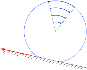
Once the drop becomes mobile, the appropriate modelling of its motion is quite challenging. In their pioneering paper, Mahadevan & Pomeau (Reference Mahadevan and Pomeau1999) argued that small non-wetting drops roll, rather than slide, when the surface is gently inclined. To elucidate this process, Mahadevan & Pomeau (Reference Mahadevan and Pomeau1999) employed the idealised notion of a perfectly non-wetting drop, where the contact angle is fixed at $180^{\circ }$. Neglecting the dynamic effect of the surrounding gas and balancing the rate of change in gravitational potential energy with an order-of-magnitude estimate for the viscous dissipation in the vicinity of the flat spot, they derived the scaling relation

(1.1)

\begin{equation} \mathcal{U} \propto \frac{\gamma \alpha}{\mu B^{1/2}}, \end{equation}

in which $\mathcal {U}$ is the drop velocity, $\alpha$ is the inclination angle, $\gamma$ is the interfacial tension and $\mu$ is the liquid viscosity; the Bond number is defined as

(1.2)

\begin{equation} B=(\kappa a)^{2}, \end{equation}

$a$ being the volume-based drop ‘radius’ and $1/\kappa =({\gamma /\rho g})^{1/2}$ the capillary length, with $\rho$ the liquid density and $g$ the gravitational acceleration. The Mahadevan–Pomeau scaling law, which counterintuitively predicts the drop speed to be inversely proportional to its size, was corroborated experimentally by Quere and coworkers. In those experiments, the perfectly non-wetting conditions assumed by Mahadevan & Pomeau (Reference Mahadevan and Pomeau1999) were approximately realised using both superhydrophobic substrates (Richard & Quere Reference Richard and Quere1999) and liquid marbles (Aussillous & Qúere Reference Aussillous and Qúere2001).

A key observation underpinning the scaling analysis of Mahadevan & Pomeau (Reference Mahadevan and Pomeau1999) is that the non-integrable stress–dissipation singularity usually associated with a moving contact line does not occur under the assumption of perfect non-wetting (Benney & Timson Reference Benney and Timson1980; Ngan & Dussan V. Reference Ngan and Dussan V1984; Benilov & Vynnycky Reference Benilov and Vynnycky2013). Thus, with that assumption, the problem of calculating the speed of a rolling droplet becomes purely hydrodynamic – there is no need to resort to ad hoc regularisations such as artificial slip, disjoining pressure, diffuse-interface models etc. To highlight the alleviation of the stress singularity, Mahadevan & Pomeau (Reference Mahadevan and Pomeau1999) derived a local solution for the flow field, close to the contact line; in doing so, they conveniently considered a two-dimensional droplet, asserting that the two problems are reasonably common.

Apart from the scaling analysis of Mahadevan & Pomeau, the hydrodynamic problem governing a rolling droplet has only been analysed in two dimensions. The focus on two dimensions may be attributed to both the availability of the local solution of Mahadevan & Pomeau and the apparent difficulties involved in analysing the three-dimensional problem. Thus, the two-dimensional counterpart of the scaling law (1.1) was identified by Hodges, Jensen & Rallison (Reference Hodges, Jensen and Rallison2004), who also claimed that a quantitative analysis would necessarily involve numerically solving for the flow field inside the drop. In fact, the hydrodynamic problem governing the rolling of a two-dimensional drop has since been solved numerically by several groups (Wang Reference Wang2008; Mognetti, Kusumaatmaja & Yeomans Reference Mognetti, Kusumaatmaja and Yeomans2010; Thampi, Adhikari & Govindarajan Reference Thampi, Adhikari and Govindarajan2013).

More recently, Yariv & Schnitzer (Reference Yariv and Schnitzer2019) carried out an asymptotic analysis of that two-dimensional problem. Following the three-dimensional scaling analysis of Mahadevan & Pomeau (Reference Mahadevan and Pomeau1999), the analysis of Yariv & Schnitzer (Reference Yariv and Schnitzer2019) focuses on the rolling regime wherein both $\alpha$ and $B$ are small. The limit $\alpha \ll 1$ allows a linearisation scheme in which the flow is solved with respect to the stationary shape of the drop. Both the stationary shape and the flow field are then analysed for $B\ll 1$ using the method of matched asymptotic expansions. On the scale of the drop, where its shape is nearly circular, the flow field is given by a rigid-body motion. This motion smoothly joins a non-trivial flow field close to the flat spot. A closed-form solution for that field was obtained in bipolar coordinates using integral transforms and residue calculus. Utilising this solution, Yariv & Schnitzer (Reference Yariv and Schnitzer2019) obtained a leading-order approximation for the drop speed. Its scaling, like $(B\ln B)^{-1}$, differs from that suggested by Hodges et al. (Reference Hodges, Jensen and Rallison2004) by the logarithmic factor, which signifies the fact that in two dimensions the dissipation on the drop scale (associated with the leading-order correction to the rigid-body motion) is actually comparable to that in the flat-spot region. Yariv & Schnitzer (Reference Yariv and Schnitzer2019) have also shown that as the contact line is approached the analytical solution for the flat-spot flow field degenerates to the local solution proposed by Mahadevan & Pomeau (Reference Mahadevan and Pomeau1999).

In this paper we carry out a comparable asymptotic analysis of the three-dimensional hydrodynamic problem. We shall thereby obtain an asymptotic solution for the flow field within the drop and thence the missing prefactor in the Mahadevan–Pomeau scaling law (1.1). Furthermore, based on our solution for the flow field, we elucidate the unique mechanism by which the contact line propagates along the surface without generating a contact-line singularity. A specific question in that context is whether the two-dimensional local solution proposed by Mahadevan & Pomeau (Reference Mahadevan and Pomeau1999) and confirmed by the analysis of Yariv & Schnitzer (Reference Yariv and Schnitzer2019) remains in some sense relevant.

Clearly, the three-dimensional rolling-drop problem is far more realistic than the two-dimensional problem analysed by Yariv & Schnitzer (Reference Yariv and Schnitzer2019). As a consequence, we shall be able to compare our asymptotic predictions with experiments. It turns out that the key to the analysis of the three-dimensional problem has to do with a remarkable feature of the flow field in the two-dimensional problem (Yariv & Schnitzer Reference Yariv and Schnitzer2019). Thus, in the vicinity of the flat spot, where the drop boundary appears planar, this field happens to satisfy the no-slip and shear-free conditions simultaneously over both the solid flat spot and the mobile fluid interface in its vicinity. This unconventional feature provides a hint for the construction of the three-dimensional solution. Conversely, we shall show that the solution method used herein, motivated by this hint, can also be used to simplify the two-dimensional analysis.

The paper is arranged as follows. The exact problem, assuming perfect non-wetting conditions, is formulated in the next section. The linearisation scheme appropriate to gentle slopes is described in § 3. The small-Bond-number limit of that scheme is analysed in § 4. The solution of the linearised-flow problem in the flat-spot region is described in § 5. Making use of this solution, the drop velocity is obtained in § 6 using a dissipation balance. The local structure of the flow in the vicinity of the moving contact line is explored in § 7. We conclude in § 8, comparing our asymptotic approximation to available experimental results and discussing the possibility of a ‘mechanistic’ calculation of the drop speed.

2. Formulation

A liquid drop (density $\rho$, viscosity $\mu$) of volume $4{\rm \pi} a^{3}/3$ is placed upon a solid plane which is inclined at an angle $\alpha$ relative to the horizontal. The contact angle is $180^{\circ }$. Our interest lies in the terminal drop velocity down the plane, denoted by $\mathcal {U}$. It is defined as the velocity of a reference system in which the flow field is steady. We neglect the dynamic effect of the surrounding air.

We employ a dimensionless formulation, normalising length variables by $a$, stress variables by $\gamma /a$ and velocity variables by $\gamma /\mu$. The dimensionless drop velocity $\mu \mathcal {U}/\gamma$ is denoted by $\omega$. 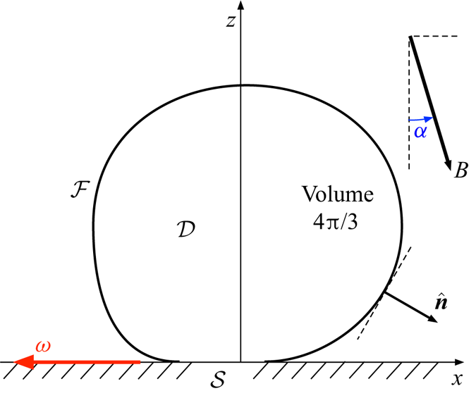(Had the drop been rotating as a rigid sphere, $\omega$ would have represented its angular velocity, normalised by $\gamma /\mu a$.) We attach the Cartesian coordinates $(x,y,z)$ to the co-moving reference frame, with the $xy$-plane coinciding with the solid plane, the $x$-axis parallel to the projection of gravity on that plane and the $z$-axis passing through the drop centroid; see figure 1. The associated position vector is $\boldsymbol {x}= x\hat {\boldsymbol {e}}_x + y\hat {\boldsymbol {e}}_y+z\hat {\boldsymbol {e}}_z$. We additionally employ the $(r,\theta ,z)$ cylindrical coordinates, defined by

(2.1a,b)

\begin{equation} x = r\cos\theta, \quad y = r\sin\theta. \end{equation}

Figure 1.

A schematic of the rolling-drop problem formulated in § 2, drawn in a co-moving reference frame. In our dimensionless notation, the body-force vector has magnitude $B$.

The drop domain is denoted by $\mathcal {D}$. Its boundary $\partial \mathcal {D}$ consists of the free surface $\mathcal {F}$ and the solid flat spot $\mathcal {S}$,

(2.2)

\begin{equation} \partial \mathcal{D} = \mathcal{F} \cup \mathcal{S}. \end{equation}

We denote by $\hat {\boldsymbol {n}}$ the outward-pointing unit normal to $\partial \mathcal {D}$; in particular,

(2.3)

\begin{equation} \hat{\boldsymbol{n}} = - \hat{\boldsymbol{e}}_z \quad \text{on} \ \mathcal{S}. \end{equation}

Volume conservation implies the constraint

(2.4)

\begin{equation} \int_{\mathcal{D}} {{\textrm{d}}V} = \frac{4{\rm \pi}}{3}, \end{equation}

where $\textrm {d}V$ is a differential volume element (normalised by $a^{3}$). The presumed $180^{\circ }$ Young angle implies that the boundary is smooth at the transition from $\mathcal {F}$ to $\mathcal {S}$, that is

(2.5)

\begin{equation} \hat{\boldsymbol{n}} \text{ is continuous at } \partial\mathcal{S}. \end{equation}

It is evident that the drop shape (and in particular $\mathcal {S}$) is symmetric about $y=0$. In general, however, no symmetry is necessitated about $x=0$.

The flow within the drop is governed by the continuity equation

(2.6)

\begin{equation} \boldsymbol{\nabla}\boldsymbol{\cdot}\boldsymbol{u} = 0 \end{equation}

and inhomogeneous Stokes equation

(2.7)

\begin{equation} \boldsymbol{\nabla} p = \nabla^{2} \boldsymbol{u} + B(\hat{\boldsymbol{e}}_x \sin\alpha - \hat{\boldsymbol{e}}_z \cos\alpha), \end{equation}

wherein $p$ is the pressure and $B=\rho g a^{2} / \gamma$ is the Bond number. Equation (2.7) may be recast in the form

(2.8)

\begin{equation} \boldsymbol{\nabla}\boldsymbol{\cdot}\boldsymbol{\sigma} + B(\hat{\boldsymbol{e}}_x \sin\alpha - \hat{\boldsymbol{e}}_z \cos\alpha) = \textbf{0}, \end{equation}

wherein

(2.9)

\begin{equation} \boldsymbol{\sigma} = -p\boldsymbol{\mathsf{I}}+2\boldsymbol{\mathsf{e}} \end{equation}

is the Newtonian stress, in which

(2.10)

\begin{equation} \boldsymbol{\mathsf{e}} = \tfrac{1}{2} [ \boldsymbol{\nabla}\boldsymbol{u} + (\boldsymbol{\nabla}\boldsymbol{u})^{\dagger}] \end{equation}

is the rate-of-strain tensor. At the free surface the flow field satisfies the stress-jump condition

(2.11)

\begin{equation} \hat{\boldsymbol{n}}\boldsymbol{\cdot}\boldsymbol{\sigma} =- \hat{\boldsymbol{n}} \boldsymbol{\nabla}\boldsymbol{\cdot}\hat{\boldsymbol{n}} \quad \text{on} \ \mathcal{F}{,} \end{equation}

while at the solid flat spot it satisfies the no-slip condition,

(2.12)

\begin{equation} \boldsymbol{u} = -\hat{\boldsymbol{e}}_x \omega \quad \text{on} \ \mathcal{S}. \end{equation}

The projection of the vectorial condition (2.12) on $\hat {\boldsymbol {e}}_z$ constitutes an impermeability condition. In fact, impermeability is satisfied over the entire fluid boundary:

(2.13)

\begin{equation} \hat{\boldsymbol{n}}\boldsymbol{\cdot}\boldsymbol{u} = 0 \quad \text{on} \ \partial \mathcal{D}. \end{equation}

It is evident that the pressure field $p$ and the $x$- and $z$-components of $\boldsymbol {u}$ are even functions of $y$, while the $y$-component of $\boldsymbol {u}$ is an odd function of $y$.

It is convenient to supplement the preceding formulation by two integral balances, which are derived from the governing equations in appendix A. The first is a force balance,

(2.14)

\begin{equation} \hat{\boldsymbol{e}}_z \boldsymbol{\cdot} \int_{\mathcal{S}} {{\textrm{d}}A} \, \boldsymbol{\sigma} = \frac{4{\rm \pi} B}{3}(\hat{\boldsymbol{e}}_x \sin\alpha - \hat{\boldsymbol{e}}_z \cos\alpha), \end{equation}

wherein ${\textrm {d}}A$ is a differential areal element. This balance represents the complete transmission of the external force to a hydrodynamic force on the solid. (This transmission, of course, is only valid for non-wetting drops.) The second is an energy budget,

(2.15)

\begin{equation} \frac{4{\rm \pi} B\omega}{3} \sin\alpha=2\int_\mathcal{D} {{\textrm{d}}V} \, \boldsymbol{\mathsf{e}} \boldsymbol{:} \boldsymbol{\mathsf{e}} ,\end{equation}

where the left-hand side represents the rate of loss of potential gravitational energy and the right-hand side the rate of dissipation of mechanical energy.

Since relations (2.14) and (2.15) follow from the governing equations, they do not provide additional independent information beyond that already contained in the problem formulation. Nonetheless, they are invaluable in the asymptotic analysis that follows.

The ultimate goal is the calculation of the drop velocity $\omega$, which appears in condition (2.12). It is a function of the two problem parameters, $\alpha$ and $B$.

3. Linearisation scheme

The hydrodynamic problem formulated in § 2 is characterised by two dimensionless parameters, the slope $\alpha$ and the Bond number $B$. In particular, that problem determines the dimensionless drop speed $\omega$ as a function of those two parameters. For gentle slopes, $\alpha \ll 1$, we anticipate that $\omega$ is proportional to $\alpha$ at leading order,

(3.1)

\begin{equation} \omega= \alpha \tilde{\omega}, \end{equation}

where $\tilde {\omega }$ is solely a function of $B$. As our interest lies in the rolling regime, where both $\alpha$ and $B$ are small, we shall aim to evaluate $\tilde {\omega }$ in the small-drop limit $B\ll 1$.

To that end, we proceed as follows. In this section we shall linearise the hydrodynamic problem of § 2 for gentle slopes ($\alpha \ll 1$), allowing for arbitrary values of $B$. The initial step in this linearisation scheme is the calculation of the reference stationary state of the drop. The linearised flow is then calculated about the geometry of that reference state. In particular, the linearisation process results in the flow being determined up to a multiplicative constant which corresponds to the rescaled drop speed $\tilde {\omega }$. This speed, in turn, is determined from the linearisation of the dissipation balance (2.15). In the subsequent section we shall focus upon the small-drop limit, $B\ll 1$, of both the stationary and linearised-flow problems.

3.1. Reference state

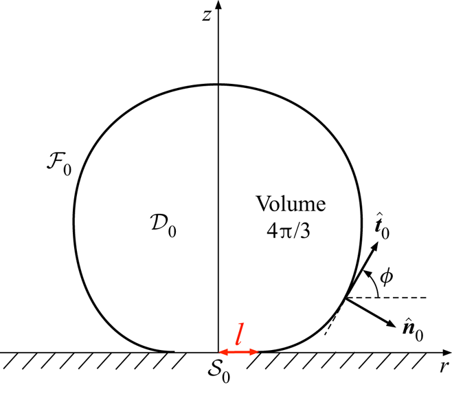
Consider first the static reference state at $\alpha =0$. The corresponding drop domain $\mathcal {D}_0$ possesses axial symmetry about the $z$-axis. It is bounded by the reference flat spot $\mathcal {S}_0$, whose unknown radius is denoted by $l$, and the reference free surface $\mathcal {F}_0$, whose outward-pointing unit normal vector is denoted by $\hat {\boldsymbol {n}}_0$ (see figure 2). The reference pressure is obtained from integration of (2.7), which readily yields the hydrostatic distribution

(3.2)

\begin{equation} p_0 = p^{*} -Bz, \end{equation}

wherein $p^{*}$ is the unknown base pressure.

Figure 2.

A schematic of the axisymmetric reference geometry (§ 3.1).

We now employ (3.2) to determine the drop shape, using an analysis in the meridian plane. Following Rienstra (Reference Rienstra1990) we employ the arc length $s$, measured from the detachment point. The surface $\mathcal {F}_0$ is parametrised using the local inclination angle $\phi$ (see figure 2), whereby $\hat {\boldsymbol {n}}_0=\hat {\boldsymbol {e}}_r \sin \phi -\hat {\boldsymbol {e}}_z\cos \phi$. The associated curvature is $\boldsymbol {\nabla }\boldsymbol {\cdot }\hat {\boldsymbol {n}}_0={\textrm {d}}\phi /{\textrm {d}}s + r^{-1}\sin \phi$. The stress balance (2.11) together with (3.2) give the Young–Laplace equation

(3.3)

\begin{equation} \frac{{\textrm{d}} {\phi}}{{\textrm{d}} {s}} + \frac{\sin\phi}{r} = p^{*}-Bz. \end{equation}

Regarding $r$ and $z$ as functions of $s$, they are governed by the differential equations

(3.4a,b)

\begin{equation} \frac{{\textrm{d}} {r}}{{\textrm{d}} {s}} = \cos\phi, \quad \frac{{\textrm{d}} {z}}{{\textrm{d}} {s}} = \sin\phi. \end{equation}

These first-order equations are supplemented by the ‘initial’ conditions

(3.5a,b)

\begin{equation} r(0) = l, \quad z(0)=0 , \end{equation}

as well as the non-wetting condition (2.5), which here reads as

(3.6)

\begin{equation} \phi(0)=0. \end{equation}

In addition, we impose two conditions. The first follows from the volume-conservation constraint (2.4), which takes the form

(3.7)

\begin{equation} \int_0^{s_M} r^{2} \frac{{\textrm{d}} {z}}{{\textrm{d}} {s}} \, {\textrm{d}} s = \frac{4}{3}, \end{equation}

wherein $s_M$ is the value attained by $s$ at the apex. The second follows from the force balance (2.14), which here reads as

(3.8)

\begin{equation} p^{*} l^{2} = \frac{4B}{3}. \end{equation}

Conceptually speaking, conditions (3.7) and (3.8) serve to determine the base pressure $p^{*}$ and detachment radius $l$.

As explained in § 2, the force-balance condition (2.14) is not independent. It may therefore appear surprising that it was used in the present context of a stationary drop to obtain the equilibrium relation (3.8). In fact, this condition conveniently replaces the regularity condition at the apex, $\phi (s_M)={\rm \pi}$, which follows from the axial symmetry. Indeed, scrutiny reveals that relation (3.8) may be alternatively obtained from integration of the Young–Laplace balance (3.3) when regularity at the apex is accounted for.

Later on, it will become convenient to employ $\phi$ as the independent variable, instead of $s$. Then (3.3) and (3.4a,b) are replaced by

(3.9a,b)

\begin{equation} \frac{{\textrm{d}} {r}}{{\textrm{d}} {\phi}} = \frac{r\cos\phi}{p^{*}r-Brz-\sin\phi}, \quad \frac{{\textrm{d}} {z}}{{\textrm{d}} {\phi}} = \frac{r\sin\phi}{p^{*}r-Brz-\sin\phi}, \end{equation}

and the volume-conservation constraint (3.7) becomes

(3.10)

\begin{equation} \int_0^{\rm \pi} r^{2} \frac{{\textrm{d}} {z}}{{\textrm{d}} {\phi}} \, {\textrm{d}}\phi = \frac{4}{3}. \end{equation}

With $r$ and $z$ now regarded as functions of $\phi$, conditions (3.5a,b) still hold.

3.2. Linearised-flow problem

Next, we employ the following small-$\alpha$ linearisation of the flow variables

(3.11a–d)

\begin{equation} \boldsymbol{u} = \alpha\tilde{\boldsymbol{u}}, \quad\boldsymbol{\mathsf{e}} = \alpha\,\tilde{\boldsymbol{\mathsf{e}}}, \quad p = p_0(z) + \alpha \tilde p, \quad \boldsymbol{\sigma} = -p_0(z) \boldsymbol{\mathsf{I}} + \alpha \tilde{\boldsymbol{\sigma}}, \end{equation}

wherein (cf. (2.9))

(3.12)

\begin{equation} \tilde{\boldsymbol{\sigma}} = -\tilde p\boldsymbol{\mathsf{I}} + 2 \tilde{\boldsymbol{\mathsf{e}}}. \end{equation}

These, in turn, imply the associated linearisation (3.1) of the drop velocity.

The problem governing the linearised flow field is naturally formulated over the stationary drop domain $\mathcal {D}_0$. Therein, the linearised flow field satisfies the continuity and inhomogeneous Stokes equations (cf. (2.6) and (2.7)),

(3.13a,b)

\begin{equation} \boldsymbol{\nabla}\boldsymbol{\cdot}\tilde{\boldsymbol{u}} = 0 ,\quad \boldsymbol{\nabla} \tilde{p} = \nabla^{2} \tilde{\boldsymbol{u}} + B \hat{\boldsymbol{e}}_x. \end{equation}

At the flat spot $\mathcal {S}_0$ it satisfies the no-slip condition (cf. (2.12)),

(3.14)

\begin{equation} \tilde{\boldsymbol{u}} = -\hat{\boldsymbol{e}}_x\tilde{\omega} \quad \text{at} \ z=0 \quad \text{for}\ r < l. \end{equation}

At the free surface $\mathcal {F}_0$ it satisfies kinematic impermeability (cf. (2.13)),

(3.15)

\begin{equation} \hat{\boldsymbol{n}}_0\boldsymbol{\cdot}\tilde{\boldsymbol{u}} = 0, \end{equation}

as well as the dynamic shear-free condition

(3.16)

\begin{equation} \hat{\boldsymbol{n}}_0\hat{\boldsymbol{t}}_0 \boldsymbol{:} \tilde{\boldsymbol{\mathsf{e}}} = 0, \end{equation}

the latter following from the projection of the stress-jump condition (2.11) on the plane tangent to $\mathcal {F}_0$ ($\hat {\boldsymbol {t}}_0$ represents any unit tangent vector in that plane).

The linearised-flow problem (3.13)–(3.16) does not by itself determine the rescaled drop speed $\tilde {\omega }$. (Indeed, for arbitrary $\tilde {\omega }$, we find a well-posed Stokes-flow problem where the normal velocity, as well as either the tangential velocity or tangential shear-stress, are prescribed over a fixed closed boundary.) Nevertheless, $\tilde {\omega }$ may be obtained from that solution using the small-$\alpha$ linearisation of the dissipation balance (2.15):

(3.17)

\begin{equation} 2\int_{\mathcal{D}_0} {\textrm{d}} V \, \tilde{\boldsymbol{\mathsf{e}}} \boldsymbol{:} \tilde{\boldsymbol{\mathsf{e}}} =\frac{4{\rm \pi} }{3}B\tilde{\omega}.\end{equation}

Since $\tilde {\boldsymbol{\mathsf{e}}}$ is proportional to $\tilde {\omega }$, this scalar constraint provides $\tilde {\omega }$ explicitly.

We emphasise that it is not possible to derive the dissipation balance (3.17) from the linearised problem (3.13)–(3.16). This may seem surprising, given that the exact dissipation balance (2.15) follows from the exact formulation in § 2. Note, however, that we have omitted from our linearised formulation the $O(\alpha )$ balances of the volume constraint (2.4) and the normal projection of the stress condition (2.11). Both involve the $O(\alpha )$ deviation of the fluid surface $\mathcal {F}$ from its reference shape $\mathcal {F}_0$, whose calculation we are inclined to avoid. For the same reason, the linearised pressure field $\tilde {p}$ is determined only up to an additive constant. (The exact problem does not involve any additive freedom in the pressure field.) Fortunately, this constant is immaterial for the purpose of calculating the velocity field and the drop speed.

For the sake of asymptotic analysis, it will also be useful to employ the $x$-component of the small-$\alpha$ linearisation of the force balance (2.14):

(3.18)

\begin{equation} \hat{\boldsymbol{e}}_x\hat{\boldsymbol{e}}_z \boldsymbol{:} \int_{\mathcal{S}_0} {\textrm{d}} A \, \tilde{\boldsymbol{\sigma}} = \frac{4{\rm \pi} B}{3}. \end{equation}

Like the linearised dissipation balance (3.17), this force balance cannot be derived from the linearised problem (3.13)–(3.16). We show in appendix A, however, that (3.17) and (3.18) are not independent; that is, one can be derived from the other using the linearised formulation.

4. Small-drop limit $B\ll 1$

In the present section we address the linearised formulation of § 3 in the small-drop limit $B\ll 1$.

4.1. Stationary reference state

We begin with the stationary reference state. Thus, integrating the Young–Laplace relations (3.9) using the volume constraint (3.10) gives, at leading order,

(4.1a–c)

\begin{equation} r=\sin\phi, \quad z =1-\cos\phi, \quad p^{*}=2. \end{equation}

The static force balance (3.8) then gives, also at leading order,

(4.2)

\begin{equation} l = (2B/3)^{1/2}. \end{equation}

Unsurprisingly, expressions (4.1a,b) describe a sphere of unity radius. Based on the form of equations (3.9), we anticipate corrections to the shape at $O(B)$. More importantly, these expressions break down near the flat spot. In what follows we consider the shape in that region, where different approximations apply.

When zooming in on the flat-spot vicinity, we need to identify the scaling of the pertinent geometric variables. With (4.2) suggesting that $r=O(B^{1/2})$, (3.9) imply that $\phi$ is of the same magnitude while $z=O(B)$. We accordingly employ the rescaled variables

(4.3a–c)

\begin{equation} \phi = B^{1/2} \varPhi, \quad r = B^{1/2} R, \quad z = B \zeta . \end{equation}

At leading order, (3.9) then provide the two first-order ordinary differential equations,

(4.4a,b)

\begin{equation} \frac{{\textrm{d}} {R}}{{\textrm{d}} {\varPhi}} = \frac{R}{2R-\varPhi} , \quad \frac{{\textrm{d}} {\zeta}}{{\textrm{d}} {\varPhi}} = \frac{R\varPhi}{2R-\varPhi} , \end{equation}

while, using (4.2), conditions (3.5) give

(4.5a,b)

\begin{equation} R(0) = \sqrt{2/3}, \quad \zeta(0)=0 . \end{equation}

In analysing the above problem, it is actually convenient to choose $R$ as the independent variable. The differential equations (4.4) thus read as

(4.6a,b)

\begin{equation} \frac{{\textrm{d}} {\varPhi}}{{\textrm{d}} {R}} = \frac{2R-\varPhi}{R} , \quad \frac{{\textrm{d}} {\zeta}}{{\textrm{d}} {R}} = \varPhi , \end{equation}

while conditions (4.5) become

(4.7a,b)

\begin{equation} \varPhi(\sqrt{2/3})=0 , \quad \zeta(\sqrt{2/3})=0 . \end{equation}

The solution of the exact differential equation (4.6a) that satisfies (4.7a) is

(4.8)

\begin{equation} \varPhi = R-\frac{2}{3R}. \end{equation}

Plugging this into (4.6b) and integrating gives, using (4.7b),

(4.9)

\begin{equation} \zeta = \frac{R^{2}}{2} - \frac{2}{3}\ln R + \frac{\ln(2/3)-1}{3}. \end{equation}

At large $R$ we find from (4.8) and (4.9) that $\varPhi \sim R$ and $\zeta \sim R^{2}/2$. These approximations simply constitute the extrapolation of the spherical shape (4.1). Note that the leading-order correction in (4.9) diverges as $\ln R$. This suggests that the correction to the spherical drop shape is in fact $O(B\ln B)$ rather than $O(B)$.

4.2. Linearised-flow problem

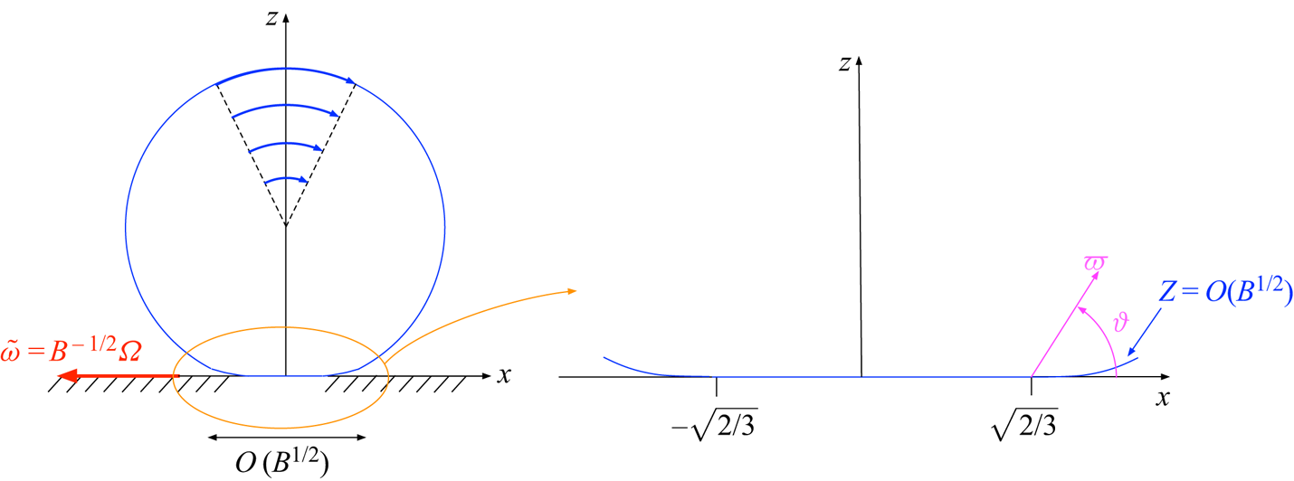
For $B\ll 1$, the reference shape of the drop is approximately spherical (recall (4.1)) except in the vicinity of the flat spot, where the meniscus is approximately flat (recall (4.3)). This scale separation is carried over to the flow analysis, where the domain $\mathcal {D}_0$ is conceptually decomposed into two regions, the ‘drop-scale region’, whose boundary is approximately spherical, and the ‘flat-spot region’, whose boundary is given by (4.9). Indeed, it is expected that in the drop-scale domain the flow is given by a rigid-body rotation. As such a rigid-body motion is incompatible with the flat spot about the origin, a separate approximation is required in the small flat-spot region (see figure 3). Given the $O(B^{1/2})$ radial scaling of that region (recall (4.3b)) and anticipating that the forced Stokes equations (3.13b) reduce there to their homogeneous form, we anticipate an $O(B^{1/2})$ extent in all directions.

Figure 3.

Flow analysis in the small-drop limit. In the drop-scale region the drop is approximately spherical, and the flow is given by the rigid-body rotation (4.11). In the flat-spot region, of $O(B^{1/2})$ extent, the meniscus shape is given by (4.9).

We begin by determining the scaling, say $\chi (B)$, of the velocity gradients within the flat-spot region. Because of asymptotic matching, that is also the scaling of the velocity gradients in the drop-scale region; with the extent of that region being $O(1)$, $\chi (B)$ also provides there the scaling of the velocity field itself. It follows that the right-hand side of (3.17) is $O(B\chi )$. The contribution of the flat-spot region to the dissipation integral on the left-hand side of (3.17) is clearly $O(B^{3/2}\chi ^{2})$. Since that contribution is expected to dominate the dissipation integral, we conclude that $\chi =B^{-1/2}$. (The above arguments constitute the dimensionless counterpart of the reasoning of Mahadevan & Pomeau Reference Mahadevan and Pomeau1999.) It is therefore convenient to write, at leading order,

(4.10)

\begin{equation} \tilde{\omega} = B^{-1/2}\varOmega, \end{equation}

$\varOmega$ thereby constituting the missing prefactor in the Mahadevan–Pomeau scaling law (1.1).

In the drop-scale region the flat spot appears as a (weak) point singularity in the limit $B\ll 1$. To leading order in $B$, the linearised flow is accordingly provided by a rigid-body motion which is consistent with (4.10):

(4.11)

\begin{equation} \tilde{\boldsymbol{u}} = B^{-1/2}\varOmega [(z-1)\hat{\boldsymbol{e}}_x - x\hat{\boldsymbol{e}}_z]. \end{equation}

This solution trivially satisfies (3.13), as well as conditions (3.15) and (3.16).

The challenge lies in the analysis of the flat-spot region. This region is naturally described in terms of the stretched coordinates (cf. (4.3b))

(4.12a–c)

\begin{equation} X = x/B^{1/2}, \quad Y=y/B^{1/2}, \quad Z = z/B^{1/2}, \end{equation}

and the associated position vector

(4.13)

\begin{equation} \boldsymbol{X} = \boldsymbol{x}/B^{1/2}= X\hat{\boldsymbol{e}}_x + Y\hat{\boldsymbol{e}}_y+Z\hat{\boldsymbol{e}}_z. \end{equation}

The corresponding cylindrical coordinates $(R,\theta ,Z)$ are defined by

(4.14a,b)

\begin{equation} X = R\cos\theta, \quad Y = R\sin\theta. \end{equation}

In view of (4.5a), the detachment curve $\partial \mathcal {S}_0$ is the circle $R=\sqrt {3/2}$ in the $XY$-plane. It follows from (4.3c) that the leading-order shape of the free surface $\mathcal {F}_0$, which initiates at this circle, is given by

(4.15)

\begin{equation} Z = B^{1/2} \zeta(R), \end{equation}

wherein $\zeta$ is given by (4.9). As this surface approaches the $XY$-plane in the limit $B\to 0$, the flat-spot region can be approximated by the upper half-space $Z>0$. (We shall soon see, however, that the small deviation (4.15) indirectly plays a crucial leading-order role.)

The $O(B^{-1/2})$ velocity gradients in conjunction with the $O(B^{1/2})$ extent of the flat-spot region imply $O(1)$ velocity variations in that region; (3.14) thus implies a combination of an $O(B^{-1/2})$ uniform velocity with an $O(1)$ spatially varying field. We accordingly write

(4.16a–d)

\begin{equation} \tilde{\boldsymbol{u}}= - \hat{\boldsymbol{e}}_x\tilde{\omega} + \varOmega \boldsymbol{U}, \quad \tilde{\boldsymbol{\mathsf{e}}} = B^{-1/2} \varOmega\boldsymbol{\mathsf{e}}, \quad \tilde p = B^{-1/2} \varOmega P, \quad \boldsymbol{\sigma} = B^{-1/2}\varOmega\boldsymbol{\varSigma}, \end{equation}

where $\tilde {\omega }$ is given by (4.10). Here,

(4.17)

\begin{equation} \boldsymbol{U} = \hat{\boldsymbol{e}}_r U + \hat{\boldsymbol{e}}_\theta V + \hat{\boldsymbol{e}}_z W, \end{equation}

is an $O(1)$ velocity field, $\boldsymbol{\mathsf{E}}$ is the symmetric part of the gradient of $\boldsymbol {U}$ with respect to the stretched position vector $\boldsymbol {X}$,

(4.18)

\begin{equation} \boldsymbol{\mathsf{e}} = \tfrac{1}{2} [\boldsymbol{\nabla}_{\boldsymbol{X}}\boldsymbol{U} + (\boldsymbol{\nabla}_{\boldsymbol{X}}\boldsymbol{U})^{\dagger}] \end{equation}

wherein

(4.19)

\begin{equation} \boldsymbol{\nabla}_{\boldsymbol{X}} = \hat{\boldsymbol{e}}_x \frac{\partial {}}{\partial {X}} + \hat{\boldsymbol{e}}_y \frac{\partial {}}{\partial {Y}} + \hat{\boldsymbol{e}}_z \frac{\partial {}}{\partial {Z}}, \end{equation}

and $\boldsymbol {\varSigma } = - P\boldsymbol{\mathsf{I}} + 2\boldsymbol{\mathsf{E}}$. Note that (i) we have conveniently factored out the expected dependence upon $\varOmega$; (ii) $\boldsymbol {U}$ constitutes the fluid velocity in the laboratory reference frame; and (iii) $\tilde {\omega }$ may also possess an $O(1)$ term, associated with a translational velocity which is comparable to $\boldsymbol {U}$. That term, however, does not play a role in the subsequent analysis.

At leading order, the flat-spot flow is governed by the homogeneous Stokes equations

(4.20a,b)

\begin{equation} \boldsymbol{\nabla}_{\boldsymbol{X}}\boldsymbol{\cdot}\boldsymbol{U} = 0 ,\quad \boldsymbol{\nabla}_{\boldsymbol{X}} P = \nabla_{\boldsymbol{X}}^{2} \boldsymbol{U} \quad \text{for} \ Z>0. \end{equation}

At large $|\boldsymbol {X}|$ it satisfies the matching condition

(4.21)

\begin{equation} \boldsymbol{U} \sim Z \hat{\boldsymbol{e}}_x - X \hat{\boldsymbol{e}}_z. \end{equation}

At $Z=0$ it satisfies the no-slip condition on $\mathcal {S}_0$, which follows from (3.14) and (4.2),

(4.22)

\begin{equation} U = V = W = 0 \quad \text{for} \ R<\sqrt{2/3}, \end{equation}

and the shear-free condition (3.16), which in view of (4.15) reads as

(4.23)

\begin{equation} \frac{\partial {U}}{\partial {Z}} + \frac{\partial {W}}{\partial {R}}=0, \quad \frac{\partial {V}}{\partial {Z}} + \frac{1}{R}\frac{\partial {W}}{\partial {\theta}}= 0\quad \text{for} \ R>\sqrt{2/3}. \end{equation}

Another condition that needs to be imposed at $Z=0$ is the free-surface kinematic condition (3.15). Some care is required, as the large velocity (4.10) necessitates to account for the small correction (4.15) to the shape of the free surface. This results in the inhomogeneous condition

(4.24)

\begin{equation} W + \frac{{\textrm{d}} {\zeta}}{{\textrm{d}} {R}} \cos\theta = 0 \quad \text{for} \ R>\sqrt{2/3}, \end{equation}

or, upon substitution of (4.9),

(4.25)

\begin{equation} W+ \left(R-\frac{2}{3R}\right)\cos\theta = 0 \quad \text{for} \ R>\sqrt{2/3}, \end{equation}

which is consistent with (4.21). (Since the shear-free condition (3.16) is independent of the $O(B^{-1/2})$ drop velocity, correction (4.15) does not affect (4.23).) For future reference, we note that relation (4.25) implies a linear variation with distance both at large $R$, where

(4.26)

\begin{equation} W\sim -R\cos\theta, \end{equation}

and close to the contact line (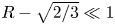$R-\sqrt {2/3}\ll 1$), where

(4.27)

\begin{equation} W\sim -2(R-\sqrt{2/3})\cos\theta. \end{equation}

Last, we postulate that the exact symmetry of the flow field about $y=0$ is enforced on the flat-spot field $\boldsymbol {U}$, which is accordingly symmetric about $Y=0$.

As it stands, the preceding problem does not uniquely determine the flat-spot velocity field $\boldsymbol {U}$. As explained further below, the problem is closed by making use of the linearised force balance (3.18), which applies at the flat-spot region. Substituting the rescaling (4.12) and (4.16d), this balance becomes homogeneous at leading order,

(4.28)

\begin{equation} \hat{\boldsymbol{e}}_x\hat{\boldsymbol{e}}_z \boldsymbol{:} \iint\limits_{\substack{Z=0\\R<({2/3})^{1/2}}} \,{\textrm{d}}X\, {\textrm{d}}Y \, \boldsymbol{\varSigma}= 0. \end{equation}

Once $\boldsymbol {U}$ is solved for, the leading-order drop velocity $\varOmega$ can be calculated from the dissipation balance (3.17). Since the dissipation is unaffected by the rigid-body motion (4.11), it is anticipated to be dominated by the flat-spot flow. At leading order, then, the balance (3.17) adopts the form

(4.29)

\begin{equation} 2\varOmega \iiint\limits_{Z>0} \boldsymbol{\mathsf{e}} \boldsymbol{:} \boldsymbol{\mathsf{e}} \, {\textrm{d}}X \, {\textrm{d}}Y \, {\textrm{d}}Z= \frac{4{\rm \pi}}{3} .\end{equation}

An implicit assumption in (4.29) is that the contribution of the leading-order correction to (4.11) is subdominant to that of the flat-spot flow. This will be verified a posteriori.

Uniqueness of the flat-spot velocity field $\boldsymbol {U}$ can be inferred by considering the difference $\boldsymbol {V}=\boldsymbol {U}_2-\boldsymbol {U}_1$ between any two solutions $\boldsymbol {U}_1$ and $\boldsymbol {U}_2$ of the flat-spot flow problem: it is obvious that $\boldsymbol {U}$ is uniquely determined if that difference vanishes identically. The velocity field $\boldsymbol {V}$ satisfies a homogeneous version of the Stokes problem governing $\boldsymbol {U}$; thus, in addition to satisfying both (4.22) and (4.23) at $Z=0$, it also satisfies the homogeneous counterpart of (4.25), implying that the vertical component of $\boldsymbol {V}$ vanishes over the entire plane $Z=0$. The far-field condition in that homogeneous version is $\boldsymbol {V}=o(|\boldsymbol {X}|)$ instead of (4.21).

We can evenly extend the problem governing $\boldsymbol {V}$ about the plane $Z=0$. (Note that this is impossible in the original problem governing $\boldsymbol {U}$.) The difference $\boldsymbol {V}$ thus represents a flow field in an infinite fluid domain external to a circular zero-width disk which is held fixed. Since the disk appears as a point singularity at large distances, the large-$|\boldsymbol {X}|$ behaviour of $\boldsymbol {V}$ can be refined by considering Lamb's general solution of the Stokes equations in spherical coordinates (Kim & Karrila Reference Kim and Karrila2005); we thereby conclude that $\boldsymbol {V}$ either attenuates in that limit or tends to a uniform stream (which, given the problem symmetry, must be in the $x$-direction).

In principle, the far-field condition (4.21) needs to be refined at this stage by higher-order matching with the drop-scale region. It is well known, however, that a uniform flow about a stationary flat disk results in a non-zero hydrodynamic force on the disk (Schnitzer & Yariv Reference Schnitzer and Yariv2018). The role of the force constraint (4.28) is thereby to rule out such non-decaying ‘eigensolutions.’ Thence the difference $\boldsymbol {V}$ attenuates at large distances. With $\boldsymbol {V}$ being additionally governed by homogeneous boundary conditions, it vanishes identically.

5. Flat-spot flow field

We look for a solution to the flat-spot flow field in the form

(5.1a,b)

\begin{equation} \boldsymbol{U}-(Z\hat{\boldsymbol{e}}_x-X\hat{\boldsymbol{e}}_z) =\hat{\boldsymbol{e}}_z\varTheta-Z\boldsymbol{\nabla}_{\boldsymbol{X}} \varTheta, \quad P = -2\frac{\partial {\varTheta}}{\partial {Z}}+ \text{constant}, \end{equation}

in which $\varTheta$ is a scalar harmonic function, odd in $Y$, that decays as $|\boldsymbol {X}|\to \infty$. This representation is a special case of the Papkovich–Neuber general solution to the Stokes equations. Clearly, it satisfies both equations (4.20) and the far-field condition (4.21). Furthermore, this representation simultaneously satisfies the no-slip and shear-free conditions at $Z=0$ for all $R>0$; accordingly, (5.1) trivially satisfies both (4.22) and (4.23) and the homogeneous force balance (4.28). The function $\varTheta$ is accordingly determined from the (inhomogeneous) kinematic condition (4.25).

Given the symmetry of the problem, we anticipate a $\cos \theta$ dependence of $\varTheta$. Writing $\varTheta = F(R,Z)\cos \theta$, representation (5.1) becomes

(5.2)

\begin{gather} \boldsymbol{U}-(Z\hat{\boldsymbol{e}}_x-X\hat{\boldsymbol{e}}_z) = \hat{\boldsymbol{e}}_zF(R,Z)\cos\theta-Z\boldsymbol{\nabla}_{\boldsymbol{X}}\left[F(R,Z)\cos\theta\right], \end{gather}

(5.3)

\begin{gather}P = -2\frac{\partial {F}}{\partial {Z}}\cos\theta+ \text{constant}. \end{gather}

The associated flow components (recall (4.17)) are

(5.4a–c)

\begin{align} U= Z\left(1-\frac{\partial {F}}{\partial {R}}\right)\cos\theta, \quad V= Z\left(\frac{F}{R}-1\right)\sin\theta,\quad W=\left(F-R-Z\frac{\partial {F}}{\partial {Z}}\right)\cos\theta. \end{align}

Since 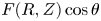$F(R,Z)\cos \theta$ satisfies Laplace's equation in the flat-spot coordinates (4.12), the function $F(R,Z)$ satisfies

(5.5)

\begin{equation} \frac{\partial {{}^{2} F}}{\partial {R^{2}}} + \frac{1}{R}\frac{\partial {F}}{\partial {R}} + \frac{\partial {{}^{2}F}}{\partial {Z^{2}}} - \frac{F}{R^{2}} = 0. \end{equation}

In addition, it satisfies the decay condition

(5.6)

\begin{equation} F\to 0 \quad \text{as} \quad |\boldsymbol{X}|\to\infty \end{equation}

and the boundary condition

(5.7)

\begin{equation} F(R,0)= \begin{cases} R, & 0 < R<\sqrt{\dfrac{2}{3}}, \\ \displaystyle \frac{2}{3R}, & R>\sqrt{\dfrac{2}{3}}, \end{cases} \end{equation}

which follows from the kinematic condition (4.25).

The above problem suggests writing $F$ as the Hankel transform

(5.8)

\begin{equation} F(R,Z)=\int_0^{\infty}kA(k)\,{\textrm{e}}^{-kZ}{\rm J}_1(kR)\,{\textrm{d}}k, \end{equation}

wherein ${\rm J}_1$ is the Bessel function of the first kind of order one; this integral representation trivially satisfies (5.5) and the decay condition (5.6). Application of the boundary conditions (5.7) then gives

(5.9)

\begin{equation} A(k)=\frac{2\sqrt{{2}/{3}}\,{\rm J}_1(k\sqrt{{2}/{3}})}{k^{2}}. \end{equation}

The far-field behaviour of the flat-spot flow is readily obtained by approximating the Hankel transform (5.8) for 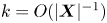$k=O(|\boldsymbol {X}|^{-1})$, obtaining

(5.10)

\begin{equation} F \sim \frac{2(1-Z/|\boldsymbol{X}|)}{3R}. \end{equation}

It then follows from (5.2) that the deviation $\boldsymbol {U}-(Z\hat {\boldsymbol {e}}_x-X\hat {\boldsymbol {e}}_z)$ from the rigid-body rotation decays like $|\boldsymbol {X}|^{-1}$. Asymptotic matching in conjunction with (4.12) thus implies that the leading-order correction to the rigid-body motion (4.11) on the drop scale is $O(B^{1/2})$. An additional correction, of the same asymptotic magnitude, follows from the interaction of the $O(B^{-1/2})$ rigid-body flow (4.11) with the $O(B)$ perturbation to the reference shape (4.1).

With that estimate, we can now systematically consider the respective contributions to the dissipation integral on the left-hand side of (3.17). Since the velocity gradient of the flat-spot flow is $O(B^{-1/2})$, the contribution of the flat-spot region is $O(B^{1/2})$. In the drop-scale region, of $O(1)$ extent, $\boldsymbol{\mathsf{E}}=O(B^{1/2})$; the contribution of that region is only $O(B)$. It follows that the integral is dominated by the flat-spot contribution. This provides the a posteriori justification for replacing (3.17) by (4.29) at leading order.

6. Dissipation balance

With the results of § 5, the flat-spot flow is presently determined up to the factor $\varOmega$ (recall (4.16)) which is the quantity of interest. We shall now calculate $\varOmega$ using the energy balance (4.29). In terms of the $(R,\theta ,Z)$ cylindrical coordinates, that balance reads as

(6.1)

\begin{equation} \frac{3\varOmega}{2{\rm \pi}}\int_0^{\infty} {\textrm{d}}R \, R \int_0^{\infty} {\textrm{d}}Z \int_0^{2{\rm \pi}} {\textrm{d}}\theta\, \boldsymbol{\mathsf{e}} \boldsymbol{:} \boldsymbol{\mathsf{e}}=1. \end{equation}

Substituting (5.2) and using the expressions for the rate-of-strain components in cylindrical coordinates (Batchelor Reference Batchelor1967), we find, for the innermost integral in (6.1),

(6.2)

\begin{align} \int_0^{2{\rm \pi}} \boldsymbol{\mathsf{e}} \boldsymbol{:} \boldsymbol{\mathsf{e}} \, {\textrm{d}} \theta &= {\rm \pi}Z^{2} \left\{\frac{3F^{2}}{R^{4}}+\frac{3}{R^{2}}\left(\frac{\partial {F}}{\partial {R}}\right)^{2} -\frac{6}{R^{3}}F\frac{\partial {F}}{\partial {R}}+\frac{2}{R^{2}}\left(\frac{\partial {F}}{\partial {Z}}\right)^{2}\right. \nonumber\\ &\quad \left. +\left(\frac{\partial {{}^{2}F}}{\partial {Z^{2}}}\right)^{2}+2\left(\frac{\partial {{}^{2}F}}{\partial {R\,\partial{Z}}}\right)^{2}+\left(\frac{\partial {{}^{2}F}}{\partial {R^{2}}}\right)^{2}\right\}. \end{align}

Using (5.5), the sum of the first three terms in the curly braces can be shown to be $3(\partial ^{2}F/\partial R^{2}+\partial ^{2}F/\partial Z^{2})^{2}$. Thus, the right-hand side of (6.2) becomes

(6.3)

\begin{equation} 2{\rm \pi} Z^{2} \left\{2\left(\frac{\partial {{}^{2}F}}{\partial {Z^{2}}}\right)^{2} +\frac{1}{R^{2}}\left(\frac{\partial {F}}{\partial {Z}}\right)^{2} + 2\left(\frac{\partial {{}^{2}F}}{\partial {R^{2}}}\right)^{2}+3\frac{\partial {{}^{2}F}}{\partial {R^{2}}}\frac{\partial {{}^{2}F}}{\partial {Z^{2}}}+\left(\frac{\partial {{}^{2}F}}{\partial {R\,\partial Z}}\right)^{2}\right\}. \end{equation}

Substitution into (6.1) gives

(6.4)

\begin{equation} {3\varPi}\varOmega = {1}. \end{equation}

Here,

(6.5)

\begin{equation} \varPi=2\varPi_\textrm{I} + \varPi_\textrm{II} + 2\varPi_\textrm{III} +3\varPi_\textrm{IV} + \varPi_\textrm{V}, \end{equation}

in which

(6.6)

\begin{gather} \varPi_\textrm{I}=\int_0^{\infty}{\textrm{d}}R\, R \int_0^{\infty} {\textrm{d}}Z\, Z^{2} \left(\frac{\partial {{}^{2}F}}{\partial {Z^{2}}}\right)^{2}, \end{gather}

(6.7)

\begin{gather}\varPi_\textrm{II}=\int_0^{\infty} \frac{{\textrm{d}}R}{R} \, \int_0^{\infty} {\textrm{d}}Z \, Z^{2}\left(\frac{\partial {F}}{\partial {Z}}\right)^{2}, \end{gather}

(6.8)

\begin{gather}\varPi_\textrm{III}=\int_0^{\infty}{\textrm{d}}R \, R \int_0^{\infty} {\textrm{d}}Z \, Z^{2} \left(\frac{\partial {{}^{2}F}}{\partial {R^{2}}}\right)^{2}, \end{gather}

(6.9)

\begin{gather}\varPi_\textrm{IV}=\int_0^{\infty} {\textrm{d}}R\, R \int_0^{\infty} {\textrm{d}}Z\, Z^{2} \frac{\partial {{}^{2}F}}{\partial {R^{2}}}\frac{\partial {{}^{2}F}}{\partial {Z^{2}}}, \end{gather}

(6.10)

\begin{gather}\varPi_\textrm{V}=\int_0^{\infty} {\textrm{d}}R\, R \int_0^{\infty} {\textrm{d}}Z \, Z^{2} \left(\frac{\partial {{}^{2}F}}{\partial {R\,\partial Z}}\right)^{2} . \end{gather}

These integrals are evaluated in appendix B, giving

(6.11)

\begin{equation} \varPi =\frac{16}{9{\rm \pi}}\sqrt{\frac{2}{3}}. \end{equation}

Substitution into (6.4) furnishes the requisite result

(6.12)

\begin{equation} \varOmega = \frac{3{\rm \pi}}{16}\sqrt{\frac{3}{2}} \approx 0.72. \end{equation}

7. Local behaviour near the contact line

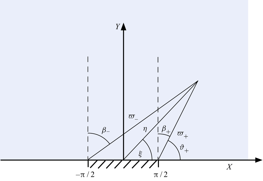
We now wish to elucidate the behaviour of the flat-spot flow in the close vicinity of the circular contact line. To this end, it is convenient to employ polar-like local coordinates in the constant-$\theta$ plane; see figure 3. These coordinates, say $\varpi$ and $\vartheta$, are defined via the relations

(7.1a,b)

\begin{equation} R-\sqrt{2/3} = \varpi \cos\vartheta, \quad Z = \varpi \sin\vartheta. \end{equation}

The behaviour near the contact line is then described by the limit $\varpi \ll 1$ of the solution obtained in the preceding section. The details are provided in appendix C, where we find

(7.2)

\begin{equation} F - \sqrt{2/3} \sim \frac{2}{\rm \pi}\varpi \ln \varpi \sin\vartheta + \varpi\left(\frac{2\vartheta}{\rm \pi}-1\right)\cos\vartheta + \frac{2-7\ln 2+\ln 3}{\rm \pi}\varpi\sin\vartheta \end{equation}

in that limit. The asymptotic error in (7.2), modulo a possible $\ln \varpi$ dependence, is $O(\varpi ^{2})$. Using (5.4), the associated leading-order radial and axial velocity components are linear in $\varpi$,

(7.3a,b)

\begin{equation} U = 2\varpi\sin\vartheta\left(1-\frac{\vartheta}{\rm \pi}\right)\cos\theta, \quad W = 2\varpi\left[ \left(\frac{\vartheta}{\rm \pi}-1\right)\cos\vartheta -\frac{\sin\vartheta}{\rm \pi} \right] \cos\theta, \end{equation}

while the associated leading-order azimuthal component is quadratic in $\varpi$ (modulo the $\ln \varpi$ dependence),

(7.4)

\begin{align} V = \sqrt{\frac{3}{2}} \varpi^{2} \left[\frac{2}{\rm \pi}\ln\varpi \sin\vartheta + 2\left(\frac{\vartheta}{\rm \pi}-1\right)\cos\vartheta + \frac{2-7\ln 2+\ln 3}{\rm \pi}\sin\vartheta\right] \sin\vartheta\sin\theta. \end{align}

With $V$ being $O(\varpi ^{2})$, the flow essentially takes place in the meridian plane perpendicular to the contact line. The flows in that plane, as given by (7.3), differs (for the same value of $\varOmega$) by a $2\cos \theta$ factor from the near-contact-line flow in the corresponding two-dimensional problem (see appendix E). We note, however, that for $\theta \mp {\rm \pi}/2 = O(\varpi )$, the azimuthal component $V$ becomes comparable to $U$ and $W$; the local flow then possesses a genuine three-dimensional structure, fundamentally different from the local flow in the two-dimensional problem.

It must be emphasised that the flow (7.3) and (7.4) constitutes a near-contact-line approximation of the linearised problem. Recalling the analogy with the comparable approximation in the corresponding two-dimensional problem (see appendix E) and the coincidence of that approximation with the local solution of Mahadevan & Pomeau (Reference Mahadevan and Pomeau1999), we conclude that the latter should not be interpreted as a local solution to the exact problem. (Indeed, it fails to satisfy the dynamic boundary condition on the meniscus.) This subtlety was not mentioned by Mahadevan & Pomeau (Reference Mahadevan and Pomeau1999).

8. Discussion

Our main result is the asymptotic approximation

(8.1)

\begin{equation} \mathcal{U}\approx \varOmega \frac{\gamma \alpha}{\mu B^{1/2}} \end{equation}

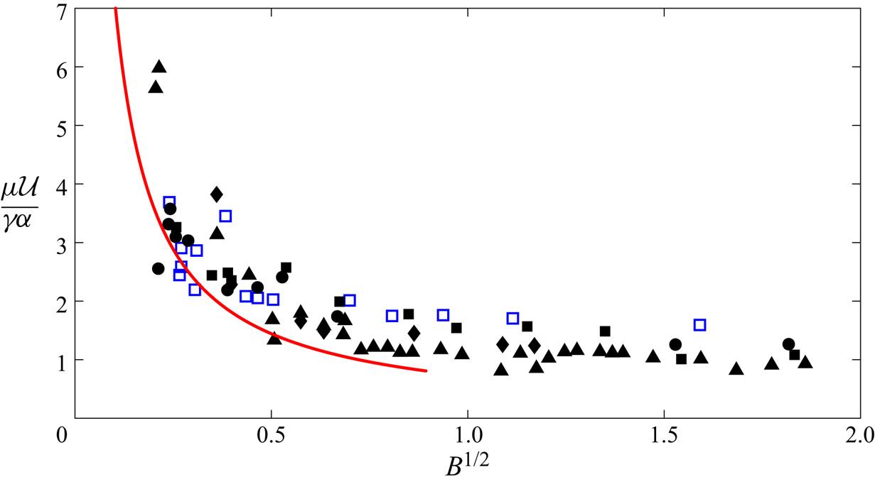
for the speed of a small non-wetting droplet rolling down a gently inclined plane, in which $\varOmega$ is given by (6.12). The constant $\varOmega$ thus provides the missing prefractor in the Mahadevan–Pomeau scaling law (1.1). In figure 4 we compare the asymptotic prediction (8.1) with experiments employing superhydrophobic surfaces (Richard & Quere Reference Richard and Quere1999) and liquid marbles (Aussillous & Qúere Reference Aussillous and Qúere2001). The asymptotic prediction is seen to be in good agreement with both sets of experiments.

Figure 4.

Normalised speed of a rolling droplet as a function of $B^{1/2}$, where the Bond number $B$ is defined in (1.2). Line: asymptotic result (8.1) with $\varOmega \approx 0.72$ given by (6.12). Empty symbols: experiments with Glycerol drops (Richard & Quere Reference Richard and Quere1999) on a superhydrophobic surface ($\alpha =13^{\circ}$). Filled symbols: experiments with ‘liquid marbles’ (Aussillous & Qúere Reference Aussillous and Qúere2001) using water and glycerol drops, two types of coating particles and with $\alpha =4$ to $8^{\circ }$.

Our analysis leading to (8.1) entailed solving for the linearised flow field in the vicinity of the flat spot of the drop. This solution, in turn, provides insight into the mechanism by which the contact line of a non-wetting droplet moves without generating a stress–dissipation singularity. Thus, we find that the shear stress is not only integrable but actually vanishes identically over the entire solid flat spot. Equally unexpectedly, the flow satisfies no-slip on the surrounding near-flat fluidic interface. It follows that the flow satisfies both no-slip and shear-free attributes over the union of the flat spot and the adjacent fluid boundary. A surprising corollary is that our leading-order result (8.1) remains valid if the physical no-slip condition on the solid flat spot is replaced by a Navier-slip condition. This may explain the agreement with experiments involving superhydrophobic surfaces, where a no-slip condition does not strictly apply.

Kinematically, the receding side of the fluid interface is ‘peeled’ upwards, with a vertical-speed distribution growing monotonically with distance from the contact line, where the vertical speed vanishes; see (4.27). The advancing side of the interface moves anti-symmetrically towards the surface. The rate of change of the vertical speed with respect to the distance from the contact line is determined by the local curvature of the stationary shape of the drop in a meridian plane normal to the contact line; see (4.25). Owing to the substantial deviation from sphericity near the flat spot, that curvature varies appreciably in the flat-spot region. In particular, the vertical speed exhibits there a non-trivial variation, growing linearly both close to and far away from the contact line (see (4.26) and (4.27)), with a nonlinear transition in between. The slope is halved through this transition, the value at large distances relative to the flat spot of course corresponding to the curvature of the unperturbed spherical drop.

Close to the near-circular contact line, the flow field primarily lies in the plane locally normal to the contact line; normalising by the drop speed, this local flow is the same as the local solution in the corresponding two-dimensional problem (see appendix E) up to a multiplicative $2\cos \theta$ factor, $\theta$ being the azimuthal angle. (This analogy breaks down near $\theta ={\pm }{\rm \pi} /2$, where the contact line propagates parallel to itself and the local flow is genuinely three dimensional.) The $\cos \theta$ factor is expected from the symmetries of the linearised three-dimensional problem. The two factor can be explained as follows. In two dimensions the curvature of the stationary drop shape remains approximately constant in the flat-spot region (Yariv & Schnitzer Reference Yariv and Schnitzer2019). With the curvature in the two-dimensional problem and the meridian curvature in the three-dimensional problem coinciding at large distances from the contact line, and given the twofold amplification of the curvature near the contact line in the three-dimensional problem, the ratio of peeling of the fluid interface to drop speed is twofold in three dimensions.

Following the scaling analysis of Mahadevan & Pomeau (Reference Mahadevan and Pomeau1999), our analysis is based on an energetic approach. That is, the rescaled drop velocity $\varOmega$ is ultimately determined using the energy budget (2.15), with the dissipation evaluated based upon our analytical solution for the flow in the flat-spot region. Is it possible to obtain $\varOmega$ by instead adopting a mechanistic approach? At least in principle, $\varOmega$ could be determined from the force balance (3.8), or, more precisely, from the linearised force balance (3.18). This balance, however, is trivial at leading order; see (4.28). We have actually used this trivial balance as a closure condition for the flat-spot problem, ensuring uniqueness of our proposed solution.

The fact that the leading-order force balance does not provide $\varOmega$ may appear to contradict the physical intuition which links drop rotation to the external forcing by gravity (which otherwise does not appear in the flat-spot problem, see (4.20b)). There is actually no contradiction: such a leading-order linkage exists, but the relevant relation is not a force balance but rather a torque balance. In fact, the Mahadevan–Pomeau scaling may be deduced from that balance, without using any energy arguments. The possibility of obtaining $\varOmega$ from the torque balance is discussed in appendix D.

Lastly, we note that our method for solving for the flat-spot flow anticipates the fact that the no-slip and shear-free conditions simultaneously hold over the union of the flat spot and the adjacent fluid boundary. This feature was also present in the analysis of the comparable two-dimensional problem (Yariv & Schnitzer Reference Yariv and Schnitzer2019). Conversely, we show in appendix E that an ansatz similar to the one used in the present three-dimensional flat-spot problem facilitates a straightforward derivation of the flat-spot flow in the comparable two-dimensional solution, which is superior to the original approach used by Yariv & Schnitzer (Reference Yariv and Schnitzer2019). This alternative derivation naturally leads to a simpler analytical form of the solution, which is easier to interpret.

Acknowledgements

E.Y. was supported by the Israel Science Foundation (grant no. 1081/16).

Declaration of interests

The authors report no conflict of interest.

Appendix A. Force and dissipation balances

We here derive the force and dissipation balances stated in § 2. While these balances appear plausible, deriving them from the governing equations is worthwhile. In particular, dissipation relations of the form (2.15) are usually derived assuming that the fluid domain is bounded by a solid boundary (Kim & Karrila Reference Kim and Karrila2005); in the present context, where the boundary contains a free surface which is subject to interfacial tension, some care is required.

To derive the force balance (2.14), we integrate the inhomogeneous Stokes equations (2.8) over $\mathcal {D}$ using Gauss theorem and (2.2) and (2.3). This gives

(A 1)

\begin{equation} \int_\mathcal{F} {\textrm{d}}A \, \hat{\boldsymbol{n}}\boldsymbol{\cdot} \boldsymbol{\sigma} - \hat{\boldsymbol{e}}_z \boldsymbol{\cdot} \int_\mathcal{S} {\textrm{d}}A \, \boldsymbol{\sigma} =- \frac{4{\rm \pi} B}{3}(\hat{\boldsymbol{e}}_x \sin\alpha - \hat{\boldsymbol{e}}_z \cos\alpha). \end{equation}

We now make use of the integral force balance on the free surface $\mathcal {F}$,

(A 2)

\begin{equation} \int_{\mathcal{F}} {\textrm{d}}A \, \hat{\boldsymbol{n}} \boldsymbol{\cdot} \boldsymbol{\sigma} = \oint_{\partial\mathcal{F}} {\textrm{d}}l \, \hat{\boldsymbol{m}}, \end{equation}

wherein ${\textrm {d}}l$ is a differential length element and $\hat {\boldsymbol {m}}$ is a unit vector which is tangential to $\mathcal {F}$ and perpendicular to $\partial \mathcal {F}$. In this balance, the left-hand side represents the hydrodynamic force due to the Newtonian stresses in the liquid, while the right-hand side represents the surface tension forces which act on the boundary $\partial \mathcal {F}$. Owing to the non-wetting condition (2.5), the vector $\hat {\boldsymbol {m}}$ is parallel to the $xy$-plane; making use of the two-dimensional variant of the gradient theorem we then find that the integral on the right-hand side of (A 2) vanishes. (This would not be the case for a wetting drop.) Substituting into (A 1), we accordingly obtain the force balance (2.14).

To derive the dissipation relation (2.15), we consider the scalar product of (2.8) and $\boldsymbol {u}$. Making use of the identity

(A 3)

\begin{equation} \boldsymbol{u}\boldsymbol{\cdot} (\boldsymbol{\nabla}\boldsymbol{\cdot}\boldsymbol{\sigma} )= \boldsymbol{\nabla}\boldsymbol{\cdot} (\boldsymbol{u}\boldsymbol{\cdot}\boldsymbol{\sigma}) - 2\boldsymbol{\mathsf{e}} \boldsymbol{:} \boldsymbol{\mathsf{e}}, \end{equation}

which readily follows from (2.9), we obtain

(A 4)

\begin{equation} \boldsymbol{\nabla}\boldsymbol{\cdot} (\boldsymbol{u}\boldsymbol{\cdot}\boldsymbol{\sigma}) - 2\boldsymbol{\mathsf{e}} \boldsymbol{:} \boldsymbol{\mathsf{e}} = -B \boldsymbol{u} \boldsymbol{\cdot} (\hat{\boldsymbol{e}}_x \sin\alpha - \hat{\boldsymbol{e}}_z \cos\alpha). \end{equation}

Integration over $\mathcal {D}$ using Gauss theorem yields

(A 5)

\begin{equation} \int_{\partial \mathcal{D}} {\textrm{d}}A\, \hat{\boldsymbol{n}} \boldsymbol{\cdot}\boldsymbol{\sigma} \boldsymbol{\cdot} \boldsymbol{u} -2\int_\mathcal{D} {\textrm{d}}V \, \boldsymbol{\mathsf{e}} \boldsymbol{:} \boldsymbol{\mathsf{e}} = -B (\hat{\boldsymbol{e}}_x \sin\alpha - \hat{\boldsymbol{e}}_z \cos\alpha)\boldsymbol{\cdot}\int_\mathcal{D} {\textrm{d}}V \, \boldsymbol{u} . \end{equation}

Making use of (2.2)–(2.3) and (2.12), the first integral on the left-hand side of (A 5) becomes

(A 6)

\begin{equation} \int_\mathcal{F} {\textrm{d}}A\, \hat{\boldsymbol{n}} \boldsymbol{\cdot}\boldsymbol{\sigma} \boldsymbol{\cdot} \boldsymbol{u} + \omega \,\hat{\boldsymbol{e}}_x \hat{\boldsymbol{e}}_z \boldsymbol{:} \int_\mathcal{S} {\textrm{d}}A\, \boldsymbol{\sigma}. \end{equation}

Given (2.11) and (2.13), the first term in (A 6) vanishes. Moreover, the continuity equation (2.6) implies that $\boldsymbol {u} = \boldsymbol {\nabla } \boldsymbol {\cdot } (\boldsymbol {u}\boldsymbol {x})$. Making use of Gauss theorem and (2.13), it follows that the right-hand side of (A 5) trivially vanishes. We conclude that

(A 7)

\begin{equation} \omega \,\hat{\boldsymbol{e}}_x \hat{\boldsymbol{e}}_z \boldsymbol{:} \int_\mathcal{S} {\textrm{d}}A\, \boldsymbol{\sigma} =2\int_\mathcal{D} {\textrm{d}}V \, \boldsymbol{\mathsf{e}} \boldsymbol{:} \boldsymbol{\mathsf{e}} . \end{equation}

Using (2.14), we then arrive at (2.15).

We conclude this appendix with a remark on (3.17) and (3.18), the small-$\alpha$ linearised forms of the exact dissipation and force balances. As discussed in § 3.2, the linearised balances cannot be derived from the linearised-flow problem (3.13)–(3.16). It is easy to see, however, that the two linearised relations are not independent in the context of that problem. Thus, repeating steps (A 4)–(A 7) above for the linearised-flow problem readily gives

(A 8)

\begin{equation} \tilde{\omega} \,\hat{\boldsymbol{e}}_x \hat{\boldsymbol{e}}_z \boldsymbol{:} \int_{\mathcal{S}_0} {\textrm{d}}A\, \tilde{\boldsymbol{\sigma}} =2\int_{\mathcal{D}_0} {\textrm{d}}V \, \tilde{\boldsymbol{\mathsf{e}}} \boldsymbol{:} \tilde{\boldsymbol{\mathsf{e}}},\end{equation}

which is just the linearised form of (A 7). Clearly, then, knowledge of the linearised force balance (3.18) yields the linearised dissipation relation (3.17) and vice versa.

Appendix B. Dissipation in the flat-spot region

In evaluating the integrals (6.6)–(6.10) we make use of the following identities:

(B 1)

\begin{gather} \int_0^{\infty}R J_\nu(k_1R)J_\nu(k_2R)\,{\textrm{d}}R= \frac{\delta(k_1-k_2)}{k_1} \quad \text{for} \quad \nu>-1, \end{gather}

(B 2)

\begin{gather}\int_0^{\infty}R^{-1}{\rm J}_1(k_1R){\rm J}_1(k_2R)\,{\textrm{d}}R=\frac{1}{2} \begin{cases} {k_1}/{k_2}, & k_1 < k_2 \\ {k_2}/{k_1}, & k_2 < k_1 \end{cases}, \end{gather}

(B 3)

\begin{gather}\int_0^{\infty}R^{-1}J_2(k_1R)J_2(k_2R)\,{\textrm{d}}R=\frac{1}{4}\begin{cases} {k_1^{2}}/{k_2^{2}}, & k_1 < k_2 \\ {k_2^{2}}/{k_1^{2}}, & k_2 < k_1 \end{cases}, \end{gather}

(B 4)

\begin{gather}\int_0^{\infty}{\rm J}_1(k_1R)J_2(k_2R)\,{\textrm{d}}R=\begin{cases} {k_1}/{k_2^{2}}, & k_1 < k_2 \\ 0, & k_2 < k_1 \end{cases}. \end{gather}

We begin with the evaluation of $\varPi _\textrm {I}$. Substituting (5.8) into (6.6) and integrating with respect to $Z$ gives

(B 5)

\begin{equation} \varPi_\textrm{I}=2\int_0^{\infty}\int_0^{\infty} {\textrm{d}}k_1 \,{\textrm{d}}k_2 \, A(k_1)A(k_2)\frac{k_1^{3}k_2^{3}}{(k_1+k_2)^{3}} \int_0^{\infty} {\textrm{d}}R \, R {\rm J}_1(k_1R){\rm J}_1(k_2R). \end{equation}

With the $R$-integral evaluated using (B 1), we obtain

(B 6)

\begin{equation} \varPi_\textrm{I}=\tfrac{1}{4}\int_0^{\infty}k^{2}A^{2}(k)\,{\textrm{d}}k, \end{equation}

or, upon substituting (5.9),

(B 7)

\begin{equation} \varPi_\textrm{I} =\frac{8}{9{\rm \pi}}\sqrt{\frac{2}{3}}. \end{equation}

Next, consider $\varPi _\textrm {II}$. Substituting (5.8) into (6.7) and integrating with respect to $Z$ gives

(B 8)

\begin{equation} \varPi_\textrm{II}=2\int_0^{\infty}\int_0^{\infty} {\textrm{d}}k_1 \,{\textrm{d}}k_2 \, A(k_1)A(k_2)\frac{k_1^{2}k_2^{2}}{(k_1+k_2)^{3}} \int_0^{\infty} \frac{{\textrm{d}} R}{R}{\rm J}_1(k_1R){\rm J}_1(k_2R). \end{equation}

With the $R$-integral evaluated using (B 2), we obtain

(B 9)

\begin{equation} \varPi_\textrm{II}=2\iint\limits_{k_1 < k_2}\frac{A(k_1)A(k_2)k_1^{3}k_2}{(k_1+k_2)^{3}}\,{\textrm{d}}k_1 \,{\textrm{d}}k_2. \end{equation}

We next calculate the integral $\varPi _\textrm {III}$. Substituting (5.8) into (6.8), making use of the identity

(B 10)

\begin{equation} \frac{{\textrm{d}} {{}^{2} {\rm J}_1(\tau)}}{{\textrm{d}} {\tau^{2}}}= \frac{J_2(\tau)}{\tau} - {{\rm J}_1(\tau)}\end{equation}

and integrating with respect to $Z$ gives

(B 11)

\begin{align} &\varPi_\textrm{III} = 2\int_0^{\infty}\int_0^{\infty} {\textrm{d}}k_1 {\textrm{d}}k_2 \, A(k_1)A(k_2)\frac{k_1^{3}k_2^{3}}{(k_1+k_2)^{3}} \nonumber\\ &\quad \int_0^{\infty} {\textrm{d}}R\, R \left[ \frac{J_2(k_1 R)J_2(k_2 R)}{k_1k_2 R^{2}} + {\rm J}_1(k_1 R){\rm J}_1(k_2 R) - \frac{{\rm J}_1(k_1 R)J_2(k_2 R)}{k_2 R} - \frac{{\rm J}_1(k_2 R)J_2(k_1 R)}{k_1 R}\right]. \end{align}

Consider the $R$-integral. Using (B 3), the contribution of the first term in the brackets to that integral is $f(k_1,k_2)/4$, where

(B 12)

\begin{equation} f(k_1,k_2)=\begin{cases} {k_1}/{k_2^{3}}, & k_1 < k_2, \\ {k_2}/{k_1^{3}}, & k_2 < k_1. \end{cases} \end{equation}

The contribution of the second term is given by (B 1). Using (B 4), the contribution of the remaining two terms in the brackets is $-f(k_1,k_2)$. Comparing with (B 6), we accordingly find

(B 13)

\begin{equation} \varPi_\textrm{III}=\varPi_\textrm{I} -3\varLambda, \end{equation}

wherein

(B 14)

\begin{equation} \varLambda = \iint_{k_1<k_2}\frac{A(k_1)A(k_2)k_1^{4}}{(k_1+k_2)^{3}}\,{\textrm{d}}k_1\, {\textrm{d}}k_2. \end{equation}

We next calculate $\varPi _\textrm {IV}$. Substituting (5.8) with (B 10) into (6.9) and integrating with respect to $Z$ gives

(B 15)

\begin{equation} \varPi_\textrm{IV} = 2\int_0^{\infty}\int_0^{\infty} {\textrm{d}}k_1 \,{\textrm{d}}k_2 \, A(k_1)A(k_2)\frac{k_1^{3}k_2^{3}}{(k_1+k_2)^{3}} \int_0^{\infty} {{\textrm{d}} R}\,{\rm J}_1(k_1 R) \left[ \frac{J_2(k_2 R)}{k_2} - R {\rm J}_1(k_2 R) \right]. \end{equation}

Using (B 1) and (B 4), the $R$-integral is

(B 16)

\begin{equation} -\frac{\delta(k_1-k_2)}{k_1} + \begin{cases} k_1/k_2^{3}, & k_1<k_2, \\ 0, & k_2<k_1 .\end{cases} \end{equation}

Integrating with respect to $k_1$ and $k_2$ and comparing with (B 6) and (B 14), we then obtain

(B 17)

\begin{equation} \varPi_\textrm{IV}= 2\varLambda - \varPi_\textrm{I}. \end{equation}

It remains to calculate $\varPi _\textrm {V}$. Substituting (5.8) into (6.10), making use of the identity

(B 18)

\begin{equation} \frac{{\textrm{d}} {{\rm J}_1(\tau)}}{{\textrm{d}} {\tau}}= \frac{{\rm J}_1(\tau)}{\tau} - J_2(\tau) \end{equation}

and integrating with respect to $Z$ gives

(B 19)

\begin{align} &\varPi_\textrm{V} = 2\int_0^{\infty}\int_0^{\infty} {\textrm{d}}k_1 \,{\textrm{d}}k_2 \, A(k_1)A(k_2)\frac{k_1^{3}k_2^{3}}{(k_1+k_2)^{3}} \nonumber\\ &\quad \int_0^{\infty} {{\textrm{d}} R}\, R \left[ \frac{{\rm J}_1(k_1 R){\rm J}_1(k_2 R)}{k_1k_2 R^{2}} + J_2(k_1 R)J_2(k_2 R) - \frac{{\rm J}_1(k_1 R)J_2(k_2 R)}{k_1 R} - \frac{{\rm J}_1(k_2 R)J_2(k_1 R)}{k_2 R} \right]. \end{align}

Making use of (B 1), (B 2) and (B 4), the $R$-integral gives

(B 20)

\begin{equation} \frac{\delta(k_1-k_2)}{k_1} -\frac{1}{2} \begin{cases} 1/k_2^{2}, & k_1<k_2, \\ 1/k_1^{2}, & k_2<k_1. \end{cases} \end{equation}

Integrating with respect to $k_1$ and $k_2$ and comparing with (B 6) and (B 9), we then obtain

(B 21)

\begin{equation} \varPi_\textrm{V}=\varPi_\textrm{I}-\varPi_\textrm{II}. \end{equation}

Upon substituting (B 13), (B 17) and (B 21) into (6.5), we find that terms involving $\varPi _\textrm {II}$ and $\varLambda$ mutually cancel, leaving $\varPi =2\varPi _\textrm {I}$. Substitution of (B 7) then gives (6.11).

Appendix C. Contact-line asymptotics

Substituting (7.1) into (5.8) gives

(C 1)

\begin{equation} F=\int_0^{\infty}kA(k) \exp({-k\varpi\sin\vartheta}){\rm J}_1(k\sqrt{2/3}+k\varpi\cos\vartheta)\,{\textrm{d}}k, \end{equation}

wherein $A(k)$ is provided by (5.9). When $\varpi =0$, we readily obtain $F = \sqrt {2/3}$. Our goal is the determination of the leading-order correction to that constant in the limit $\varpi \to 0$. In attempting to obtain that correction by a Taylor expansion of the integrand about $\varpi =0$ we encounter a diverging integral. It turns out that the limit $\varpi \to 0$ corresponds here to an ‘intermediate’ case where the dominant contribution to the integral is neither local nor global (Hinch Reference Hinch1991).

We accordingly use the method of splitting, temporarily introducing a cutoff-like parameter $\lambda$:

(C 2)

\begin{equation} F=\left(\int_0^{\lambda}+\int_{\lambda}^{\infty}\right)kA(k) \exp({-k\varpi\sin\vartheta}){\rm J}_1(k\sqrt{2/3}+k\varpi\cos\vartheta)\,{\textrm{d}}k.\end{equation}

Since the arbitrary parameter $\lambda$ is at our disposal, we can choose it at will. To begin with, we require that it satisfies

(C 3)

\begin{equation} 1\ll \lambda\ll\varpi^{-1}. \end{equation}

Consider the ‘local’ contribution to $F$, given by the first integral in (C 2). Since $k\varpi$ is small in the integration domain, we can employ Taylor expansions. This gives

(C 4)

\begin{align} &\int_0^{\lambda} k A(k) \{ {\rm J}_1(k\sqrt{2/3})+\varpi [(\cos\vartheta\sqrt{3/2}- k\sin\vartheta){\rm J}_1(k\sqrt{2/3})\nonumber\\ &\quad -kJ_2(k\sqrt{2/3})\cos\vartheta] + \cdots\}\,{\textrm{d}}k. \end{align}

Integrating and expanding for $\lambda \gg 1$ gives

(C 5)

\begin{align} &\left\{\sqrt{\frac{2}{3}}-\frac{2}{{\rm \pi}\lambda} +O\left(\frac{1}{\lambda^{2}}\right)\right\} \nonumber\\ &\quad + \varpi\left\{-\frac{1}{\rm \pi}\left(2\ln \lambda +2\gamma-4+\ln \frac{128}{3}\right)\sin\vartheta + O\left(\frac{1}{\lambda^{1/2}}\right)\right\} + \cdots . \end{align}

Consistency requires that the asymptotic errors are subdominant to the smallest terms retained; the original requirement (C 3) is accordingly modified to

(C 6)

\begin{equation} \varpi^{-1/2}\ll\lambda\ll \varpi^{-1}. \end{equation}

Consider now the ‘global’ contribution to $F$, given by the second integral in (C 2). Using the change-of-variables $s=\varpi k$ and substituting (5.9) gives

(C 7)

\begin{equation} 2\sqrt{\frac{2}{3}}\int_{ \varpi\lambda}^{\infty}s^{-1}\exp({-s\sin\vartheta}){\rm J}_1 (s\sqrt{2/3}/\varpi){\rm J}_1(s\sqrt{2/3}/\varpi+s\cos\vartheta)\,{\textrm{d}}s. \end{equation}

Making use of the large-argument asymptotic behaviour of the Bessel function,

(C 8)

\begin{equation} {\rm J}_1(\tau) \sim \left(\frac{2}{{\rm \pi}\tau}\right)^{1/2} \cos(\tau-3{\rm \pi}/4) + O(\tau^{-3/2}), \end{equation}

we obtain at leading order

(C 9)

\begin{align} &\frac{4\varpi}{\rm \pi}\int_{ \varpi\lambda}^{\infty}s^{-2}\exp({-s\sin\vartheta}) \cos(2s\sqrt{2/3}/\varpi\nonumber\\ &\quad -3{\rm \pi}/4) \cos(2s\sqrt{2/3}/\varpi +s\cos\vartheta -3{\rm \pi}/4)\,{\textrm{d}}s, \end{align}

which involves the product of ‘rapidly’ oscillating cosines of slightly different frequencies. The key to the asymptotic evaluation of (C 9) is suggested by the ‘beating’ phenomenon (Benson Reference Benson2006). Thus, the idea is to transform this product to the sum of ‘slow’ and ‘fast’ cosines, whereby (C 9) becomes

(C 10)

\begin{align} \frac{2\varpi}{\rm \pi}\int_{ \varpi\lambda}^{\infty}s^{-2}\exp({-s\sin\vartheta})\left[\cos(s\cos\vartheta)+\cos(2s\sqrt{2/3}/\varpi +s\cos\vartheta -3{\rm \pi}/2)\right]{\textrm{d}}s. \end{align}

The ‘slow’ contribution to the integral in (C 10) is written as the sum

(C 11)

\begin{equation} \int_{\varpi\lambda}^{\infty}s^{-2}\exp({-s\sin\vartheta}) \, {\textrm{d}}s + \int_{\varpi\lambda}^{\infty} s^{-2}\exp({-s\sin\vartheta}) \left[ \cos(s\cos\vartheta)-1\right]{\textrm{d}}s . \end{equation}

For small $\varpi \lambda$, the first integral in (C 11) is

(C 12)

\begin{equation} \frac{1}{\varpi\lambda} + \left[\gamma_E-1+\ln(\varpi\lambda) + \ln \sin\vartheta\right] \sin\vartheta + o(1), \end{equation}

wherein $\gamma _E$ is the Euler–Mascheroni constant. Since the integrand of the second integral in (C 11) is $O(1)$ for small $s$, we may replace at leading order the lower integration limit $\varpi \lambda$ by $0$; this gives for that integral

(C 13)

\begin{equation} \left(\vartheta-\frac{\rm \pi}{2}\right)\cos\vartheta-\ln(\sin\vartheta)\sin\vartheta + o(1). \end{equation}

Adding up (C 12) and (C 13) yields the ‘slow’ contribution to the integral in (C 10),

(C 14)

\begin{equation} \frac{1}{\varpi\lambda} + \left[\gamma_E-1+\ln(\varpi\lambda) \right] \sin\vartheta + \left(\vartheta-\frac{\rm \pi}{2}\right)\cos\vartheta + o(1). \end{equation}

Using the standard method of integration by parts (Bender & Orszag Reference Bender and Orszag1978), it is readily seen that the comparable contribution of the ‘fast’ Fourier-like integral in (C 10) is of order $\varpi ^{-1}\lambda ^{-2}$; given (C 6), it is subdominant to (C 14). We conclude that, for small $\varpi \lambda$, the global contribution (C 9) gives

(C 15)

\begin{equation} \frac{2}{{\rm \pi}\lambda}+\frac{2\varpi}{\rm \pi}\left\{[\gamma_E-1+\ln(\varpi\lambda)] \sin\vartheta + \left(\vartheta-\frac{\rm \pi}{2}\right)\cos\vartheta\right\} + o(\varpi). \end{equation}

Adding the above global contribution to the local contribution (C 5), we find that all the terms that involve $\lambda$ are cancelled out, as they should. This results in the requisite approximation (7.2).

Appendix D. Torque balance

An integral torque balance of the exact problem may be obtained following the lines of the derivation of the integral force balance (see appendix A). We start by defining the drop centre-of-mass position $\bar {\boldsymbol {x}}$ as

(D 1)

\begin{equation} \frac{4{\rm \pi}}{3} \bar{\boldsymbol{x}} = \int_{\mathcal{D}} \boldsymbol{x} \, {\textrm{d}}V. \end{equation}

It follows from the problem symmetry and the choice of coordinate system in § 2 that

(D 2)

\begin{equation} \bar{\boldsymbol{x}} = \hat{\boldsymbol{e}}_z \bar{z}. \end{equation}

Next, forming the vector product of $\boldsymbol {x}$ with the inhomogeneous Stokes equations (2.8) gives

(D 3)

\begin{equation} \boldsymbol{x} \boldsymbol{\times} (\boldsymbol{\nabla}\boldsymbol{\cdot}\boldsymbol{\sigma}) + B[(z\hat{\boldsymbol{e}}_y-y\hat{\boldsymbol{e}}_z) \sin\alpha - \hat{\boldsymbol{e}}_z (x\hat{\boldsymbol{e}}_y-y\hat{\boldsymbol{e}}_x)\cos\alpha] = \textbf{0}. \end{equation}

Integration over $\mathcal {D}$ using Gauss theorem and (D 1) and (D 2) yields

(D 4)

\begin{equation} \oint_{\partial\mathcal{D}} {\textrm{d}}A \, \boldsymbol{x} \boldsymbol{\times} (\hat{\boldsymbol{n}} \boldsymbol{\cdot}\boldsymbol{\sigma}) + \hat{\boldsymbol{e}}_y \frac{4{\rm \pi} B}{3} \bar{z}\sin\alpha = \textbf{0}. \end{equation}

Making use of (2.2) and (2.3) thus gives

(D 5)

\begin{equation} \int_{\mathcal{F}} {\textrm{d}}A \, \boldsymbol{x} \boldsymbol{\times} (\hat{\boldsymbol{n}} \boldsymbol{\cdot}\boldsymbol{\sigma}) - \int_{\mathcal{S}} {\textrm{d}}A \, \boldsymbol{x} \boldsymbol{\times} (\hat{\boldsymbol{e}}_z \boldsymbol{\cdot}\boldsymbol{\sigma}) =- \hat{\boldsymbol{e}}_y\frac{4{\rm \pi} B}{3} \bar{z}\sin\alpha . \end{equation}

We now employ the integral torque balance on the free surface $\mathcal {F}$ (cf. (A 2)),

(D 6)

\begin{equation} \int_{\mathcal{F}} {\textrm{d}}A \, \boldsymbol{x} \boldsymbol{\times} (\hat{\boldsymbol{n}} \boldsymbol{\cdot} \boldsymbol{\sigma}) = \oint_{\partial\mathcal{F}} {\textrm{d}}l \, \boldsymbol{x} \boldsymbol{\times} \hat{\boldsymbol{m}}. \end{equation}

Noting that $\hat {\boldsymbol {m}}$ is parallel to the $xy$-plane and making use of the two-dimensional variant of Gauss theorem, we find that the integral on the right-hand side of (D 6) vanishes. We accordingly obtain the torque balance

(D 7)

\begin{equation} \int_{\mathcal{S}} {\textrm{d}}A \, \boldsymbol{x} \boldsymbol{\times} (\hat{\boldsymbol{e}}_z \boldsymbol{\cdot}\boldsymbol{\sigma}) = \hat{\boldsymbol{e}}_y\frac{4{\rm \pi} B}{3} \bar{z} \sin\alpha. \end{equation}

Unsurprisingly, only the $y$-component of (D 7) is non-trivial. Upon substituting the Newtonian expression (2.9) for $\boldsymbol {\sigma }$ and making use of the no-slip condition (2.12), that component becomes

(D 8)

\begin{equation} \int_\mathcal{S} {\textrm{d}}A \, x p = \frac{4{\rm \pi} B}{3} \bar{z} \sin\alpha . \end{equation}

For $\alpha \ll 1$, we find that both the left- and right-hand sides of (D 8) are $O(\alpha )$. Naívely, the linearisation of (D 8) may appear to give, using (3.11c),

(D 9)

\begin{equation} \iint_{\mathcal{S}_0}x \tilde{p} \, {\textrm{d}}x \, {\textrm{d}}y = \frac{4{\rm \pi} B}{3} \bar{z} . \end{equation}

Using the flat-spot scaling in the limit $B\ll 1$, we find that both sides of (D 9) are $O(B)$. (In fact, one could have obtained the scaling (4.10) from the dominant balance of (D 9).) In that limit, moreover, where $\mathcal {D}$ is approximately spherical, $\bar {z}$ is unity at leading order. We accordingly obtain

(D 10)

\begin{equation} \varOmega\iint\limits_{\substack{Z=0\\R<({2/3})^{1/2}}}X P \, {\textrm{d}}X \, {\textrm{d}}Y = \frac{4{\rm \pi}}{3}, \end{equation}

or, in polar coordinates,

(D 11)

\begin{equation} \varOmega\int_0^{2{\rm \pi}}{\textrm{d}}\theta \cos\theta \int_0^{\sqrt{2/3}} {\textrm{d}}R \,R^{2} \left.P\right|_{Z=0} = \frac{4{\rm \pi}}{3}. \end{equation}

Upon substituting (5.3), we find that the unknown constant in that expression makes no contribution. We therefore obtain

(D 12)

\begin{equation} -2\varOmega \int_0^{\sqrt{2/3}} {\textrm{d}}R \,R^{2} \left.\frac{\partial {F}}{\partial {Z}}\right|_{Z=0} = \frac{4}{3}. \end{equation}

Substituting (5.8) and (5.9) gives for the left-hand side of (D 12),

(D 13)

\begin{equation} 4\sqrt{\tfrac{2}{3}} \varOmega \int_0^{\sqrt{2/3}} {\textrm{d}}R \,R^{2} \int_0^{\infty} {\textrm{d}}k \, {\rm J}_1(k\sqrt{{2}/{3}}) {\rm J}_1(kR) . \end{equation}

Performing the integration and substitution into (D 12) eventually furnishes the result

(D 14)

\begin{equation} \varOmega = \frac{3{\rm \pi}}{4}\sqrt{\frac{3}{2}}, \end{equation}

which differs from (6.12) by a factor of $4$.

The discrepancy has to do with a term that has been overlooked in (D 9). In general, the $O(\alpha )$ shape perturbation implies an $O(\alpha )$ deviation of $\mathcal {S}$ from the disk $\mathcal {S}_0$. The left-hand side of (D 9) must therefore incorporate an additional term that represents the torque associated with the action of the hydrostatic pressure on that deviation. While the hydrostatic pressure is uniform at $z=0$, that term would not vanish if the deviation is asymmetric about $x=0$. (In principle, the shape perturbation may also result in an $O(\alpha )$ deviation of $\bar z$ from unity. This, however, does not affect the linearised balance (D 9).)

The calculation of the $O(\alpha )$ shape perturbation is a formidable task which we have deliberately avoided. While the torque balance does in principle set $\varOmega$, the dissipation balance approach is vastly superior. The situation encountered herein is reminiscent of the classical problem of high-Reynolds-number flow about a gas bubble, where a dissipation balance readily yields the drag about a translating bubble (Levich Reference Levich1962). In that problem, the ‘mechanistic’ calculation of the drag using a direct stress integration posed a long-standing challenge (Moore Reference Moore1963) that was eventually overcome by Kang & Leal (Reference Kang and Leal1988).

Appendix E. Flat-spot flow field in the two-dimensional problem

In the two-dimensional problem the velocity gradients are $O(B^{-1})$, rather than $O(B^{-1/2})$. In this problem (4.10) and (4.16) are respectively replaced by

(E 1)

\begin{equation} \tilde{\omega} = B^{-1}\varOmega, \end{equation}

and

(E 2a–d)

\begin{equation} \tilde{\boldsymbol{u}} = -\hat{\boldsymbol{e}}_x \tilde{\omega} + \varOmega \boldsymbol{U}, \quad \tilde{\boldsymbol{\mathsf{e}}} = B^{-1} \varOmega\boldsymbol{\mathsf{e}}, \quad \tilde p = B^{-1} \varOmega P, \quad \boldsymbol{\sigma} = B^{-1}\varOmega\boldsymbol{\varSigma}. \end{equation}

The flat-spot flow $\boldsymbol {U}$ is now of the form $\hat {\boldsymbol {e}}_x U + \hat {\boldsymbol {e}}_y V$, where $U$ and $V$ are functions of $X$ and $Y$. (Note that in factoring out $\varOmega$ in (E 2) there is a slight difference compared with the notation of Yariv & Schnitzer (Reference Yariv and Schnitzer2019).) The flat-spot flow $(\boldsymbol {U},P)$ is governed by the homogeneous Stokes equations. At $Y=0$ the boundary conditions depend upon the location on the $X$-axis. On the flat spot, where $|X|<{\rm \pi} /2$, the flow satisfies impermeability and no-slip,

(E 3a,b)

\begin{equation} V=0, \quad U=0. \end{equation}

At the free surface, which corresponds to $|X|>{\rm \pi} /2$, the flow satisfies the shear-free condition

(E 4)

\begin{equation} \frac{\partial {U}}{\partial {Y}} +\frac{\partial {V}}{\partial {X}}=0 \end{equation}

and the impermeability condition

(E 5)

\begin{equation} V = \pm{\rm \pi}/2 -X \quad \text{for} \ X\gtrless{\rm \pi}/2, \end{equation}

which is inhomogeneous. In addition, the flow must match the outer rigid-body rotation

(E 6a,b)

\begin{equation} U \sim Y, \quad V \sim - X \quad \text{for} \ |\boldsymbol{X}|\gg 1. \end{equation}

Following the analysis of § 5 we look for a solution in the form

(E 7)

\begin{equation} \boldsymbol{U}-(Y\hat{\boldsymbol{e}}_x-X\hat{\boldsymbol{e}}_y) =\hat{\boldsymbol{e}}_y\varTheta-Y\boldsymbol{\nabla}_{\boldsymbol{X}} \varTheta, \end{equation}

where $\varTheta$ is a scalar harmonic function. With the above representation, the no-slip and shear-free conditions at $Y=0$ are satisfied for all $X$, implying that both (E 3b) and (E 4) are trivially satisfied. In terms of $\varTheta$, the kinematic conditions (E 3a) and (E 5) read as

(E 8)

\begin{equation} \varTheta(X,0) = \begin{cases} X, & |X|<{\rm \pi}/2,\\ \pm{\rm \pi}/2, & X\gtrless{\rm \pi}/2. \end{cases}\end{equation}

We write $\varTheta$ as a sine transform,

(E 9)

\begin{equation} \varTheta(X,Y) = \int_0^{\infty} B(k) \,{\textrm{e}}^{-k Y} \sin kX \, {\textrm{d}}k. \end{equation}

Application of (E 8) gives

(E 10)

\begin{equation} B(k) = \frac{2}{\rm \pi}\frac{\sin{\rm \pi} k/2}{k^{2}}. \end{equation}

Using (E 9) and (E 10), the velocity component $U$ is

(E 11)

\begin{equation} U = Y - Y\frac{\partial {\varTheta}}{\partial {X}} = Y \left\{1-\frac{1}{\rm \pi}\left[ \arctan \frac{X+{\rm \pi}/2}{Y}-\arctan\frac{X-{\rm \pi}/2}{Y}\right]\right\}. \end{equation}

Defining the ‘offset’ polar coordinates (see figure 5)

(E 12a,b)

\begin{equation} \varpi_\pm^{2} = (X\mp{\rm \pi}/2)^{2}+Y^{2}, \quad \beta_\pm = \arctan \frac{X\mp{\rm \pi}/2}{Y}, \end{equation}

we obtain a more convenient representation

(E 13)

\begin{equation} U = Y \left(1+\frac{\beta_+-\beta_-}{\rm \pi}\right). \end{equation}

The velocity component $V$ is

(E 14)

\begin{equation} V = - X +\varTheta - Y\frac{\partial {\varTheta}}{\partial {Y}} = -X + \frac{1}{\rm \pi}\left[\left(X+\frac{\rm \pi}{2}\right)\beta_- - \left(X-\frac{\rm \pi}{2}\right)\beta_+\right]. \end{equation}

Defining the streamfunction $\varPsi$,

(E 15a,b)

\begin{equation} U-Y = \frac{\partial {\varPsi}}{\partial {Y}}, \quad V+X = -\frac{\partial {\varPsi}}{\partial {X}}, \end{equation}

we obtain

(E 16)

\begin{equation} \varPsi = \frac{\varpi_+^{2}\beta_+ - \varpi_-^{2}\beta_-}{2{\rm \pi}} - \frac{Y}{2} + \frac{{\rm \pi}^{2}}{4}, \end{equation}

where the constant is chosen to nullify $\varPsi$ at the points $(\pm {\rm \pi}/2,0)$. Scrutiny reveals that (E 16) indeed agrees with (7.16) in Yariv & Schnitzer (Reference Yariv and Schnitzer2019), which provides a closed-form expression for the streamfunction in terms of bipolar coordinates.

Figure 5.

Coordinates used in the flat-spot analysis of the two-dimensional problem.

We can easily obtain a local approximation to the flow near the ‘right’ contact point $({\rm \pi} /2,0)$. To that end, it is convenient to employ the polar angle (see figure 5)

(E 17)

\begin{equation} \vartheta_+ = \frac{\rm \pi}{2}- \beta_+, \end{equation}

in terms of which $X={\rm \pi} /2+\varpi _+ \cos \vartheta _+$. Noting that, for small $\varpi _+$,

(E 18)

\begin{equation} \beta_- \sim \frac{\rm \pi}{2} - \frac{\varpi_+ \sin\vartheta_+}{\rm \pi} + O(\varpi_+^{2}), \end{equation}

we readily obtain from (E 13) and (E 14),

(E 19a,b)

\begin{equation} U \sim \varpi_+ \left(1-\frac{\vartheta_+}{\rm \pi}\right)\sin\vartheta_+, \quad V \sim \varpi_+ \left[ \left(\frac{\vartheta_+}{\rm \pi}-1\right)\cos\vartheta_+ -\frac{\sin\vartheta_+}{\rm \pi} \right], \end{equation}

with an $O(\varpi _+^{2})$ asymptotic error. In the three-dimensional problem the $r$ and $z$ cylindrical coordinates are approximately Cartesian coordinates close to the contact line. Comparing the corresponding approximations for the velocity components (as given by (7.3)) to approximations (E 19), we readily observe the similarity between the two local fields (see (7.4) et seq.).

We can also obtain a far-field approximation. To that end, it is convenient to employ the polar coordinates $\eta$ and $\xi$, defined via the relations (see figure 5),

(E 20a,b)

\begin{equation} X = \eta\cos\xi, \quad Y = \eta\sin\xi. \end{equation}

Making use of the large-$\eta$ expansions,

(E 21a,b)

\begin{equation} \varpi_\pm^{2} \sim \eta^{2} \mp{\rm \pi} \eta \cos\xi + O(1), \quad \beta_\pm \sim \frac{\rm \pi}{2} - \xi \mp \frac{{\rm \pi}\sin\xi}{2\eta} + O(\eta^{-2}), \end{equation}

we find that the $O(\eta ^{2})$ terms in (E 16) cancel out, leaving the $O(\eta )$ approximation,

(E 22)

\begin{equation} \varPsi \sim -\eta\left[\sin\xi + \left(\frac{\rm \pi}{2}-\xi\right)\cos\xi\right] \quad \text{as} \ \eta\to\infty. \end{equation}

With $\varPsi$ being $O(\eta )$, the deviation of $\boldsymbol {U}$ from the rigid-body-rotation profile does not decay as $\eta \to \infty$. Rather,

(E 23a,b)

\begin{equation} \lim_{\eta\to\infty}\{U- Y\} = - \sin^{2}\xi, \quad \lim_{\eta\to\infty}\{V+X\}=\sin\xi\cos\xi + \frac{\rm \pi}{2}-\xi. \end{equation}

The uniqueness arguments of § 4.2 are easily adapted in the two-dimensional problem. (This issue was overlooked by Yariv & Schnitzer Reference Yariv and Schnitzer2019.) Consulting Lamb's general solution of the Stokes equations in two dimensions (Kim & Karrila Reference Kim and Karrila2005) we find that, at large $\eta$, the ‘difference’ field $\boldsymbol {V}$ either decays or diverges as $\ln \eta$. The last behaviour is ruled out by the condition of zero force in the $x$-direction (namely the equivalent of (4.28) in the two-dimensional problem). With $\boldsymbol {V}$ attenuating at large distances and otherwise satisfying homogeneous boundary conditions, it vanishes identically. The velocity field obtained via representation (E 7) accordingly constitutes the unique solution to the flat-spot problem.

References

REFERENCES

Aussillous, P. & Qúere, D. 2001 Liquid marbles. Nature 411 (6840), 924–927.CrossRef Google Scholar PubMed

Batchelor, G. K. 1967 An Introduction to Fluid Dynamics. Cambridge University Press.Google Scholar

Bender, C. M. & Orszag, S. A. 1978 Advanced Mathematical Methods for Scientists and Engineers. McGraw-Hill.Google Scholar

Benilov, E. S. & Vynnycky, M. 2013 Contact lines with a

$180^{\circ }$ contact angle. J. Fluid Mech. 718, 481–506.CrossRef Google Scholar

Benney, D. J. & Timson, W. J. 1980 The rolling motion of a viscous fluid on and off a rigid surface. Stud. Appl. Maths 63 (2), 93–98.CrossRef Google Scholar

Benson, D. 2006 Music: A Mathematical Offering. Cambridge University Press.CrossRef Google Scholar

Hinch, E. J. 1991 Perturbation Methods. Cambridge University Press.CrossRef Google Scholar

Hodges, S. R., Jensen, O. E. & Rallison, J. M. 2004 Sliding, slipping and rolling: the sedimentation of a viscous drop down a gently inclined plane. J. Fluid Mech. 512, 95–131.CrossRef Google Scholar

Kang, I. S. & Leal, L. G. 1988 The drag coefficient for a spherical bubble in a uniform streaming flow. Phys. Fluids 31, 233–237.CrossRef Google Scholar

Kim, S. & Karrila, S. J. 2005 Microhydrodynamics: Principles and Selected Applications. Dover.Google Scholar

Levich, V. G. 1962 Physicochemical Hydrodynamics. Prentice-Hall.Google Scholar

Mahadevan, L. & Pomeau, Y. 1999 Rolling droplets. Phys. Fluids 11 (9), 2449–2453.CrossRef Google Scholar

Mognetti, B. M., Kusumaatmaja, H. & Yeomans, J. M. 2010 Drop dynamics on hydrophobic and superhydrophobic surfaces. Faraday Discuss. 146, 153–165.CrossRef Google Scholar PubMed

Moore, D. W. 1963 The boundary layer on a spherical gas bubble. J. Fluid Mech. 16 (2), 161–176.CrossRef Google Scholar

Ngan, C. G. & Dussan V, E. B. 1984 The moving contact line with a

$180^{\circ }$ advancing contact angle. Phys. Fluids 27 (12), 2785–2787.CrossRef Google Scholar

Quéré, D., Azzopardi, M.-J. & Delattre, L. 1998 Drops at rest on a tilted plane. Langmuir 14 (8), 2213–2216.CrossRef Google Scholar

Richard, D. & Quere, D. 1999 Viscous drops rolling on a tilted non-wettable solid. Europhys. Lett. 48 (3), 286–291.CrossRef Google Scholar

Rienstra, S. W. 1990 The shape of a sessile drop for small and large surface tension. J. Engng Maths 24 (3), 193–202.CrossRef Google Scholar

Schnitzer, O. & Yariv, E. 2018 Small-solid-fraction approximations for the slip-length tensor of micropillared superhydrophobic surfaces. J. Fluid Mech. 843, 637–652.CrossRef Google Scholar

Thampi, S. P., Adhikari, R. & Govindarajan, R. 2013 Do liquid drops roll or slide on inclined surfaces? Langmuir 29 (10), 3339–3346.CrossRef Google Scholar PubMed

Wang, X. 2008 On the rolling motion of viscous fluid an a rigid surface. PhD thesis, Institute of Technology, New Jersey.Google Scholar

Yariv, E. & Schnitzer, O. 2019 Speed of rolling droplets. Phys. Rev. Fluids 4 (9), 093602.CrossRef Google Scholar

Figure 1.A schematic of the rolling-drop problem formulated in § 2, drawn in a co-moving reference frame. In our dimensionless notation, the body-force vector has magnitude $B$.

Figure 2.A schematic of the axisymmetric reference geometry (§ 3.1).

Figure 3.Flow analysis in the small-drop limit. In the drop-scale region the drop is approximately spherical, and the flow is given by the rigid-body rotation (4.11). In the flat-spot region, of $O(B^{1/2})$ extent, the meniscus shape is given by (4.9).

Figure 4.Normalised speed of a rolling droplet as a function of $B^{1/2}$, where the Bond number $B$ is defined in (1.2). Line: asymptotic result (8.1) with $\varOmega \approx 0.72$ given by (6.12). Empty symbols: experiments with Glycerol drops (Richard & Quere 1999) on a superhydrophobic surface ($\alpha =13^{\circ}$). Filled symbols: experiments with ‘liquid marbles’ (Aussillous & Qúere 2001) using water and glycerol drops, two types of coating particles and with $\alpha =4$ to $8^{\circ }$.

Figure 5.Coordinates used in the flat-spot analysis of the two-dimensional problem.

Article contents

Rolling of non-wetting droplets down a gently inclined plane

Abstract

JFM classification

Information

1. Introduction

2. Formulation

3. Linearisation scheme

3.1. Reference state

3.2. Linearised-flow problem

4. Small-drop limit $B\ll 1$

4.1. Stationary reference state

4.2. Linearised-flow problem

5. Flat-spot flow field

6. Dissipation balance

7. Local behaviour near the contact line

8. Discussion

Acknowledgements

Declaration of interests

Appendix A. Force and dissipation balances

Appendix B. Dissipation in the flat-spot region

Appendix C. Contact-line asymptotics

Appendix D. Torque balance

Appendix E. Flat-spot flow field in the two-dimensional problem

References

REFERENCES

Save article to Kindle

Save article to Dropbox

Save article to Google Drive

Reply to: Submit a response

Your details

You have entered the maximum number of contributors

Conflicting interests