Since the Brundtland Commission report (World Commission on Environment and Development, 1987), the potential to advance both economic growth and environmental quality has been a major focus of debate and analysis within and beyond the economics profession. Grossman and Krueger (Reference Grossman and Krueger1995) placed the issue in sharp relief by documenting empirical relationships between national income levels and industrial pollutants. For several of these pollutants, they discovered a pattern that has become known as the environmental Kuznets curve (EKC): as income grows, both emissions and ambient concentrations first rise and then fall, generating an inverted U-shaped relationship. Recent studies suggest that the EKC may prevail in the time domain, but does not seem to be a robust result in the cross-sectional/longitudinal domain.Footnote 1 We thus, focus on a dynamic theory of the EKC.
The EKC is a correlation in search of an underlying theoretical explanation. Moreover, the rise and fall of pollution in different economies might be governed by markedly different economic forces as in the cases of market and transition economies.Footnote 2 A better understanding of these differences might shed light into effective policies under different institutional settings, and provide theoretical guidance to empirical studies on growth and the environment. This is the main goal of our paper.
Following the tradition of two-sector endogenous growth models with an initial imbalance in capital, we develop a simple dynamic model of economic growth and environmental quality.Footnote 3 Our analysis is distinctive in two important respects. First, we provide a stylized framework for the unified treatment of both typical western market economies and the transition economies of the former Soviet Bloc. These economies are characterized by their ratio of capital to environmental quality relative to an optimal benchmark. Our results show how the EKCs for these two groups draw on different driving forces, thus providing additional theoretical guidance to empirical papers on the growth–environment literature. To the best of our knowledge, this unified treatment is the first of its kind. Second, we introduce an environmental protection function that incorporates expenditures designed to correct two common sources of market failure: a pollution externality, and the existence of a public good that can be optimally provided at a cost. The public good is environmental quality, and involves expenditures on actions such as reforestation, habitat restoration, carbon sequestration, and re-introduction of species. We thus allow for the correction of a pollution externality at each time, as well as investments in the increase of the stock of the environment. Other papers in the literature overlook the latter policy option,Footnote 4 which, as we show, affects the optimal choice of policy instruments in a decentralized economy.
A number of other results emerge from our analysis. First, the optimal time path of environmental expenditures mimics the stylized fact that public commitment to environmental protection is characterized by discrete shifts in most market economies. In the US, for example, environmental regulation and the related expenditures grew sharply in the late 1960s and 1970s with the passage of a suite of new environmental laws (Portney, Reference Portney1990). This phenomenon is captured in our model by benign neglect of the environment when capital is relatively scarce and a discrete jump in environmental expenditures after the economy reaches the optimal balance between capital and the environment.Footnote 5 Second, the fraction of output spent on environmental protection is constant during a balanced growth phase of the economy with increasing environmental quality. Both the rapid increase in expenditures and the relatively stable fraction of output devoted to environmental protection seem to agree with the data on pollution abatement and control expenditures for the US in recent decades (US Bureau of the Census, 1996). Third, because there are two sources of market failure in our economy, a pollution externality and the public good environmental quality, neither a Pigouvian tax nor tradable pollution permits can, in general, implement the Pareto optimum. These instruments are meant to correct only the pollution externality distortion. One of the two has to be accompanied by a consumption tax to finance optimal provision of environmental quality. Furthermore, grandfathering of tradable pollution allowances also fails to generate enough revenues to implement the social optimum. Finally, the model predicts that after environmental quality reaches an upper bound, environmental protection expenditures represent a constant but smaller fraction of output and are solely devoted to correction of the pollution externality. From this point on, resources saved on environmental protection are shifted to consumption.
The driving force for the EKC in our formulation of a market economy is similar to that in Selden and Song (Reference Selden and Song1995), Stokey (Reference Stokey1998), and Lieb (Reference Lieb2002). At early stages of economic development, the relatively high marginal rate of substitution of consumption for environmental quality implies decreasing environmental quality, a trend that is eventually reversed as capital accumulates and consumption grows. A distinctive feature of our model, however, is that the EKC in market economies is solely driven by the relative scarcity of capital to environmental quality, and does not require any restrictions on the elasticity of marginal utility of consumption (as in Stokey, Reference Stokey1998), intergenerational conflicts of interest (John and Pecchenino, Reference John and Pecchenino1994), and property rights and institutions (Chichilnisky, Reference Chichilnisky1994; López, Reference López1994; Bohn and Deacon, Reference Bohn and Deacon2000).
The paper proceeds as follows: section 1 describes the model; section 2 investigates its interior solution; section 3 analyzes the transition to the steady state for our representation of both market and transition economies; section 4 addresses policies for directing a decentralized market and transition economy along the optimal path; section 5 explores a generalization of the utility function and shows how the EKC does not depend on the elasticity of marginal utility and is optimal even when we relax the assumption of balanced growth. Section 6 draws conclusions.
1. Model
Consider an economy modeled in continuous time t where each of the N identical individuals values consumption of a private good, ct, and a pure public good, environmental quality, Et. We assume that instantaneous individual utility is given by

where α is between zero and one. Individuals have a constant discount rate 0 < ρ < 1.
Let Kt be the aggregate capital stock at time t. Output, Yt, is produced using capital according to a linear technology, Yt ≡ F(Kt) = AKt, where A > 0. Pollution, P(Kt), is a by-product of production, reduces environmental quality, and is a linear function of capital, P(Kt) = PKt, where P > 0.Footnote 6 However, society can mitigate the effects of pollution by spending πt ≥ 0 on environmental protection. These expenditures are of two types: expenditures on the correction of the instantaneous pollution externality, such as end-of-the-pipe pollution abatement; and expenditures on the optimal provision of the public good environmental quality beyond contemporaneous pollution control. Accordingly, environmental quality evolves over time according to Ė t = −PK t + Ππt, where Π > 0 is the aggregate technological parameter for the productivity of environmental protection expenditures.
It might be tempting to interpret Ππt as pollution abatement and the expression −PKt + Ππt as the net flow of emissions at time t. This is not the case here, though. The variable πt includes not only pollution abatement at time t, but also expenditures on recovery of degraded areas, development of nature reserves, protection of endangered species, etc. That is, in contrast to other modelsFootnote 7 environmental expenditures not only include correction of the pollution externality through abatement of the flow of pollutants at time t, but also the optimal provision of the public good environmental quality through recovery and improvement of the stock of the environment. In that sense, the qualitative results remain unchanged if we replace πt in the environmental protection function with πβ1tπ1−β2t, where π 1t are expenditures on pollution abatement, π 2t are other expenditures on environmental protection, and 0 < β < 1. More generally, the environmental protection function exhibits diminishing returns in each type of environmental protection expenditure, but aggregate constant returns to scale. Appendices A and B contain the results comparable to those below, but allowing for more than one type of environmental protection expenditure.
Finally, output can be used for aggregate consumption, environmental protection, and investment in physical capital: F(Kt) = AKt = Nct + πt + It. Capital depreciates at the constant rate 0 < δ < 1, so that capital accumulation is given by:  t = I t − δK t or t = AK t − Nc t − πt − δK t. We assume that the standard transversality condition holds: limt →∞e−ρtμtKt = 0, where μt is the current value of the shadow value of capital.
In a centralized economy, a social planner maximizes per capita lifetime utility by choosing paths for consumption and environmental protection that solve

subject to the initial conditions K 0 and E 0, the laws of motion for environmental quality and capital accumulation

and the non-negativity constraints πt ≥ 0, I t ≥ 0, and Ē − E t ≥ 0 whenever Ė > 0, where Ē ≤ E p, and Ep is the pristine environment. Ē < E p captures irreversible environmental damages, and the upper bound on Et applies only when environmental quality is increasing. That is, once environmental quality was degraded below a sufficiently large Ē it can increase again through corrective actions, but it can never again exceed this limit.
The necessary conditions for a maximum are

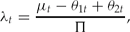
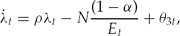




and the transversality condition

where μt is the shadow value of capital,  is a constant, λt is the shadow value of environmental quality, θ 1t, θ 2t ≥ 0 capture the non-negativity of environmental protection expenditures and physical capital investment, respectively, and θ 3t captures the upper bound on environmental quality.
At the optimum, equation (1) shows that the marginal contribution of capital to social welfare must equal the marginal utility from additional consumption produced with the extra unit of capital. Equation (2) indicates the optimal trade-off between the stock of environmental quality and the stock of capital, taking the marginal cost of improving environmental quality and the slackness conditions into consideration.
Equations (3) and (4) form a system of differential equations with the laws of motion governing the shadow values of environmental quality and capital. At any given time, the rate of change in the shadow value of environmental quality is positively related to the discount rate and negatively related to the marginal utility of environmental quality. In an interior solution, changes in the shadow value of the stock of capital are positively related to the cost of marginal pollution in terms of environmental quality, the discount rate and the depreciation rate, and negatively related to the marginal product of capital.
2. Balanced growth
In a balanced growth economy, every variable of the system grows at the same constant rate. Assuming an interior solution to the maximization problem above, the associated necessary conditions and the transversality condition are given in equations (1) through (8) with θ 1t = θ 2t = θ 3t = 0. The results for the balanced growth path are summarized below. Full derivations are available from the authors.
The resulting optimal rate of growth of consumption is constant:  . Assuming that the marginal product of capital is high enough to cover the marginal environmental protection cost per unit of capital, the discount rate, and the capital depreciation rate, consumption will increase with time.
The necessary conditions also require a constant ratio between consumption and environmental quality at each time t:  or, in more compact notation, Et = ɸct. This expression is the Samuelson condition for the optimal provision of the public good environmental quality. It shows that the marginal rate of substitution between consumption and environmental quality is constant along the balanced growth path of the economy and can be rewritten as:

These results, the initial conditions and the laws of motion for Kt and Et, and the transversality condition give the optimal path of the state and control variables of the model


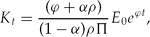

Equation (12) can be rewritten as  That is, expenditures on environmental protection are a function of aggregate consumption and the flow of pollution (PKt) at time t. The second term on the right-hand side of the above expression corresponds to the revenues from the pricing of pollution in a decentralized economy, whereas the first term refers to the additional resources needed for the optimal provision of the public good environmental quality. Proposition 2 shows that the term multiplying Nct is the tax rate on consumption, whereas 1/Π is the Pigouvian tax on pollution (PKt).
All variables in equations (9)–(12) grow at the same rate γ*, characterizing a balanced growth path for the economy: γ*c = γ*π = γ*K = γ*E = γ* = ϕ. As a consequence, the ratio between the control and state variables is constant at each time t. In particular, from (9) and (11), the ratio between the stocks of capital and environmental quality is
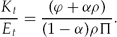
Clearly, in general, (13) will not hold with equality at t 0. Thus, analysis of the transitional dynamics from the initial conditions to balanced growth becomes a relevant exercise. But, before turning to the transitional dynamics, it is interesting to investigate the economy beyond balanced growth, that is after the upper bound on environmental quality is reached and the constraint represented by equation (7) is binding.
2.1. Beyond balanced growth
Assume that there is a finite date t 1 where the ratio between capital and environmental quality satisfies equation (13). Thereafter, environmental quality will grow exponentially at the rate ϕ until it reaches the upper bound Ē at some finite date t 2. That is, for t ≥ t 2, E t = Ē, implying that θ 3t > 0, Ė t = 0 and  . Manipulation of the first-order conditions for the social planner's maximization problem gives the path for capital, consumption, and environmental protection expenditures

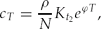
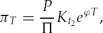
where the time index is redefined such that T = t − t 2 ≥ 0.
The interpretation of equation (16) is analogous to the interpretation of (12), except that after the upper bound on environmental quality is reached the only optimal expenditures on environmental protection relate to the correction of the contemporaneous pollution externality, and not to further increases of the stock of the environment. Thus, the right-hand side of (16) is simply the Pigouvian tax revenues.
The rate of growth for these variables remains the same as along the balanced growth path. Since we rule out infinite rates of investment or disinvestment in capital, the stock of capital is continuous in time. Thus, for t > t 2,  and
 is given by equation (11). Aggregate consumption and environmental protection expenditures, on the other hand, experience discrete jumps of the same magnitude and opposite signs at date t 2:

This result is intuitive. At time t 2, environmental quality reaches its upper bound. From that date on, Ė t = 0 and Et stays at its maximum Ē. To sustain zero growth of environmental quality all that is required is that the pollution externality from capital be corrected without further investment in environmental protection. That is, a smaller fraction of output needs to be devoted to environmental protection relative to the case along the balanced growth path of the economy, when Ė t > 0. With constant environmental quality, expenditures on environmental protection correspond to pollution tax revenues in a decentralized economy and are given by (16), where the right-hand side is pollution times its marginal damage, 1/Π, or the Pigouvian fee. The resources saved from the movement from positive to zero growth of environmental quality can now be shifted to consumption.
3. Transitional dynamics
This section turns to consider the transitional path to balanced growth induced by an imbalance on the initial conditions for capital and environmental quality. We first analyze the case where the initial ratio of capital to environmental quality is smaller than the optimal ratio in (13). We call an economy with such an imbalance a market economy. Most market-driven economies, such as the US and Western European countries, are rooted in a past when environmental quality was abundant relative to the stock of productive capital. In addition, we analyze the opposite type of imbalance − the initial ratio of capital to environmental quality is larger than the optimal ratio in (13). The transition economies of the former Soviet Bloc, when transition began in earnest, departed from a condition of abundant productive capital (especially as we broadly define capital to include physical and human capital) and a poor state of the environment.
Consider a country starting its process of economic development with a small stock of capital (i.e. small K 0) and a pristine environment (i.e. large E 0). In terms of equation (13),  . The social planner wishes to bring the economy to the balanced endogenous growth path described in section 2, therefore changing the initial ratio of capital to environmental quality so as to achieve equality in (13). One way to achieve this goal is to destroy part of the environmental stock and convert it into capital so that equality in (13) is immediately achieved. However, immediate conversion of the stock of the environment into capital is only possible, and even then, only to a limited extent, in extractive societies. It is more realistic to assume that these jumps are negligible and can be approximated by finite positive rates of investment in Kt and finite negative rates of growth of Et. Negative growth in Et will result from a simultaneous increase in the capital stock and pollution along with zero expenditures on environmental protection.
Under these circumstances, the social planner recognizes the relative scarcity of capital and its relatively high shadow value, thus increasing the stock of capital and allowing environmental quality to decrease. That is, with a relatively large stock of environmental quality, the shadow value of the environment, λt, is zero − society is not willing to spend any resources on an additional unit of environmental quality. This, along with positive investment in the stock of capital implies that θ2t = 0 and θ1t = μt > 0. Furthermore, from equation (4), the shadow value of capital decays faster when θ1t = μt > 0

Equation (17) is consistent with higher rates of growth observed at earlier stages of development, when the capital stock of the economy is small relative to its environmental stock.
Manipulation of the necessary conditions produces the optimal paths for capital, consumption, and environmental quality during the transition to the optimal ratio of capital to environmental quality

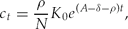

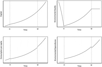
As environmental quality decreases according to (20), Et is concave in t, highlighting increasing environmental degradation. The transition to balanced growth is complete at the finite date t 1. At that time, the social planner faces a larger stock of capital, and consequently more pollution, than at t 0. To offset pollution and promote environmental improvements along the optimal balanced growth path, a discrete jump from zero to strictly positive environmental expenditures  is required. This result mimics the stylized fact that most developed market oriented economies experienced a strong process of innovation in institutions for environmental protection and significant increase in environmental expenditures starting in the 1960s. Furthermore, capital and consumption begin to grow at a reduced rate, indicating, as some commentators suggest, that environmental protection is a drag on income growth as conventionally measured (see for example, Denison, Reference Denison1985; Jorgenson and Wilcoxen, Reference Jorgenson and Wilcoxen1990; Stokey, Reference Stokey1998).Footnote 8 Proposition 1 summarizes these results.
Definition 1Environmental quality is abundant at time t if and only if the ratio of capital to environmental quality is smaller than the optimal balanced growth path ratio, i.e.  .
We will use the notion of abundant capital stock when we discuss a model for the transition economies of Eastern Europe, but will not formally define abundant capital, since it follows immediately from definition 1.
Proposition 1For a country starting its planning horizon with abundant environmental quality:
(i) environmental quality is decreasing and concave in time during the transition to the balanced growth economy. Furthermore, the transition to the long-term state of the environment takes a finite period of time − there are finite times t 1and t 2such that environmental quality is increasing at the rate ϕfor every t 1 ≤ t < t 2, and constant for every t ≥ t 2;
(ii) the rate of growth of consumption from t 0to t 1, γc, exceeds its (constant) rate of growth ϕat dates t ≥ t 1. Furthermore, ct is discontinuous at t 1and t 2

(iii) environmental expenditures πtare: (a) zero from t 0 to t 1, and then (b) increasing at the constant rate ϕat dates t ≥ t 1. Furthermore, πtis discontinuous at t 1and t 2




Proof: See appendix B. □
From proposition 1(iii), environmental expenditures have two components along the balanced growth solution. The last term corresponds to the Pigouvian tax revenues meant to correct the pollution externality in a decentralized economy. The first term represents the sacrifices consumers are required to make to finance the optimal provision of the public good environmental quality to compensate for its degradation.
Figure 1 summarizes the results from proposition 1 and section 2. It illustrates the Pareto optimal paths from environmental quality, environmental expenditures, consumption, and capital in an economy starting its planning horizon with abundant environmental quality. These paths are consistent with the EKC and the delayed environmental expenditures in most countries. Additionally, since capital and environmental expenditures grow at the same rate after date t 1, the results imply that the fraction of output devoted to environmental protection is relatively large and constant for t 1 < t < t 2, and relatively small and constant for t > t 2. Data on environmental protection for the US are available from 1972 to 1994 and suggest a significant increase in the ratio of environmental expenditures to GDP in the first four years of the sample followed by a stable ratio in subsequent years (US Bureau of the Census, Reference Grossman and Krueger1996; Brock and Taylor, Reference Brock, Taylor, Durlauf and Aghion2005). Furthermore, our model predicts that, everything else constant, this ratio should decrease but remain strictly positive when the opportunities vanish for growth in environmental quality.
Capital, Environmental Quality, Consumption per capita and Environmental Expenditures

The market economy results do not apply universally. The transition economies of the former Soviet Bloc demark the other polar case, where capital is abundant (albeit inefficiently used) and environmental quality is scarce. We broadly define capital to include human capital, thus lending further support to our AK formulation. Observations for several Eastern European countries in the late 1980s and early 1990s report pollution and energy intensities of GDP that were well above those of most market-driven economies at comparable income levels.Footnote 9 Chimeli (Reference Chimeli2003) explored this case in detail, so we briefly summarize his results here.Footnote 10
Consider an economy with a relatively abundant stock of productive capital at t 0. That is,  . Starting with a relatively large stock of capital the optimal ratio of capital to environmental quality along the balanced growth path of the economy can be reached in finite time. As with market economies, infinite rates of disinvestment in capital or investment in the environment are ruled out, so that the non-negativity constraint on investment in capital is binding and θ2t > 0. Equivalently, the social planner recognizes the relatively low shadow value of capital and allows the capital stock to depreciate at the exogenous rate δ: t = −δK t, that is total output is exhausted with consumption and environmental protection at each time t during the transition, implying that πt = Ae −δtK 0 − Nct. Under these circumstances, the social planner can reach the optimal ratio of capital to environmental quality in finite time (Chimeli, Reference Chimeli2003: 137): ‘For every
 , there is a
 and a time t* < ∞ such that the initial conditions (ω0, χ0) imply
 .
The formal proof of this result implicitly defines a policy that is sufficient but not necessary for the social planner to reach the optimal ratio of capital to environmental quality in finite time. The intuition is that given  , the social planner will reduce investment in capital accumulation down to zero. Furthermore, output can be split at t 0 in a way biased towards low consumption and relatively large expenditures on environmental protection. The exponential decay of the stock of capital (and consequently of pollution) combined with expenditures of total output biased towards investment in environmental protection will lead
 to zero as time goes to infinity, implying that there is a time t* when the ratio of capital to environmental quality reaches the optimal ratio from above. At this time, the social planner switches to the balanced growth solution with strictly positive investment in capital and environmental protection as characterized in section 2. In general, Chimeli's result defines a family of paths leading to the completion of the transitional dynamics in finite time.Footnote 11
Strictly speaking, our results for transition economies map the latter portion of their EKC, when environmental quality improves. The first portion of the EKC in this case comes from the socialist era, when the policy objectives differed from social welfare maximization.Footnote 12 We emphasize that, although market and transition economies may experience EKC-like paths for environmental quality, their EKCs stem from two distinct phenomena with distinct driving forces, a result that can be of relevance to empirical applications. For example, our approach recommends against an econometric model that uses a simple dummy variable to differentiate transition economies from their market-oriented counterparts. Such a model implicitly assumes different levels of the same underlying mechanism for the growth–environment relationship in both cases, which is not an appropriate practice according to our framework.
A note on dynamic rationalityFootnote 13
The discrete jumps in consumption described in proposition 1 and figure 1 imply discrete jumps in utility. Forward-looking economic agents would forecast these jumps and adjust their consumption paths to smooth consumption over time. In this sense, proposition 1 relies on unforeseen regime changes at times t 1 and t 2. This could result from agents whose behavior combines elements of rationality and bounded rationality. Economic agents rationally respond to the incentives they face at each period under consideration (0 < t < t 1, t 1 < t < t 2 and t > t 2), but fail to anticipate the regime changes associated with environmental policy.Footnote 14
We can address time consistency in our model by imposing a continuity condition on consumption.Footnote 15 As we do this, the main results of the paper do not change: (1) the capital-scarcity driven EKC still results (proposition 1(i)); (2) consumption grows at a slower rate after society starts to spend on environmental protection (proposition 1(ii)); (3) expenditures on environmental protection are discontinuous (proposition 1(iii)), which parallels the stylized fact that attention to environmental protection is a comparatively late phenomenon in more developed economies relative to correction of other sources of market failure (delayed investment in one stock variable is also common in two-sector growth models with an initial imbalance involving the stocks of physical and human capital);Footnote 16 and (4) the policy instruments to implement Pareto optimality are unchanged (proposition 2 below).
Consumption smoothing would impose a cost to our analysis, though. First, the derivations for the expressions for the variables of the model increase in complexity without providing further intuition on the results. Second and most importantly, the interior solution involving gains in environmental protection no longer traces a balanced growth path for the variables of the model. In particular, expenditures on environmental protection as a percentage of income changes over time. This seems to be at odds with currently available information.Footnote 17 We, therefore, take the view that ‘not insisting on consistency with rational expectations is justified as a short-cut that, for the question at hand, appears to cost little’ (Sargent, Reference Sargent1993: 28–29). In other words, the framework we propose in the paper is a simpler way to analyze the research question we want to address.
4. Decentralized economy
In this section, we follow Stokey (Reference Stokey1998) and analyze the problem of implementing the Pareto optimal solution by solving for the choice of policy instruments in a decentralized economy. In particular, we focus on a pollution tax, tradable pollution permits, a pollution standard, and a consumption tax. We consider the cases when either environmental quality or capital is initially abundant.
The typical economic instruments to correct a pollution externality are a pollution tax or tradable pollution permits, but one of these instruments alone will not suffice to implement the social optimum in our economy. A well-known result applies here: Pareto optimality requires a different policy instrument for the correction of each source of market failure. A pollution tax corrects the pollution externality by inducing firms to choose the socially optimal level of pollution, and a consumption tax ensures financing of the optimal provision of the public good environmental quality. We assume that total tax revenues are fully spent on the provision of environmental quality, that is we assume a government that runs a balanced budget and is costless to operate.
To verify this result, consider a decentralized economy where representative households hold capital, which they rent to firms and whose returns are used for consumption, payment of consumption taxes, and savings. They maximize the stream of the overall utility from t 0 to infinity, subject to the law of motion for capital. Formally, their problem is

subject to

where r is the rental rate of capital, τc is the tax on consumption, and νt is the current-value shadow value of capital.
The firms' problem is static and, because the technology exhibits constant returns to scale, the industry can be represented by a single firm. At each time t, each firm faces a tax on pollution, τp, and chooses capital to maximize profits

Proposition 2 derives a policy rule to implement the socially optimal solution in this economy. Let 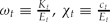 and
 , and define the policy vector τ = (τp, τc).
Proposition 2In a decentralized economy, the policy rule to implement the Pareto optimal solution is such that:
(i) For every time t such that ωt < ω*, τ = (0, 0);
(ii) For every time t such that ωt > ω*,
, where xt = (1+τct), and ;(iii) for every t such that ωt = ω*,
; and(iv) for every t such that condition (7) is binding,
.
 , where xt = (1+τct), and
 ;
 ; and
 .
Proof: See appendix B. □
Proposition 2 defines the optimal policy rules for the implementation of the Pareto optimal solution for our economy as a function of a tax on pollution and a tax on consumption. The variable ω*is the optimal ratio of capital to environmental quality from equation (13). Thus, case (i) shows that benign neglect of environmental protection (tax rates are zero) is the optimal policy when capital is scarce relative to environmental quality in market economies. Case (ii) defines the combination of tax rates along the transition to the optimal ratio of Kt to Et in a transition economy. Case (iii) gives the optimal constant tax rates along the balanced growth path of the economy, when the optimal ratio of Kt to Et is attained. Finally, after environmental quality is driven to its upper bound in case (iv), the Pigouvian tax corrects the contemporaneous pollution externality and the optimal consumption tax rate becomes zero, since there is no room for further increases in the stock of the environment.
We can also show the well-known result that the Pareto optimal solution can be implemented with tradable pollution permits, and the equilibrium permit price is equal to the optimal pollution tax. However, optimality will result if and only if the government sells permits at their equilibrium price during the balanced growth phase, or if the government fully taxes profits generated by granting firms free pollution permits. Freely distributed permits cannot implement the Pareto optimum since in this case the government would not collect enough revenues to optimally provide the public good, environmental quality. In contrast to this paper, most of the optimal growth literature overlooks this result. The reason for this is that other studies typically rule out restoration activities that can increase the stock of environmental quality (or decrease the stock of pollution).Footnote 18 Our model incorporates expenditures such as those involving ecosystem recovery, species re-introduction, reforestation, etc. The failure of freely distributed pollution permits to produce Pareto optimality follows directly from proposition 2.
Corollary 1Freely distributed pollution permits coupled with consumption taxes cannot implement the Pareto optimal solution.
Proof: See appendix B. □
Finally, suppose the government enforces a pollution standard, thus imposing a limit on the stock of capital to be used at each time t, and sets a consumption tax as before.Footnote 19 The households' problem remains the same and the firm's zero-profit condition implies that r = A − δ. This rental price differs from that from the first-best solution and Pareto optimality will not result. The intuition for the failure of a pollution standard to implement the optimum in a dynamic economy is well explained by Stokey (Reference Stokey1998: 24):
With a pollution tax . . . emissions have a market price that is entirely separate from the return to capital. Hence the market return to capital is an accurate measure of the incremental value of investment and provides the correct incentive to save. With direct regulation, ownership of capital brings with it the right to emit a specified level of pollution. Thus, the market return to capital is the sum of its real economic return and the value of the associated pollution rights. The bundled price overstates the return to investment and provides the wrong incentives for accumulation.
The extension of the results from this section to the case of more than one type of environmental protection expenditure, each exhibiting diminishing returns, but with aggregate constant returns follows easily (see appendix B).
5. Constant elasticity of substitution utility
In this section, we generalize the utility function to show how the EKC does not depend on the elasticity of marginal utility and is optimal even when we relax the assumption of balanced growth.Footnote 20 Consider a more general utility function with constant elasticity of intertemporal substitution, given by

where Ψ, Λ, σ, and η are positive constants. The preceding analysis refers to the case when Ψ = α, Λ = 1−α, and σ, η → 1.
To avoid unnecessary complications, we only focus on the linear environmental protection function Ππt. The case when the environmental protection function is given by Ππβ1tπ1−β2t can be analyzed as before and will not be pursued here. The interior solution to the social planner's problem gives

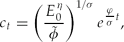


where  and we assume that σ, η, ϕ, and ρ are such that all the variables of the model are positive and increase along the optimal path.
Furthermore, the ratio of capital to environmental quality is given by

Therefore, the optimal path for the economy results only if at t 0 the ratio of capital to environmental quality is constant and equal to:

As in the previous case, this is not true in general, and the EKC-like path for the environment results from the social planner's problem if environmental quality is abundant at t 0. Expenditures on environmental protection are zero from t 0 to t 1 and positive and increasing afterwards. Likewise, the case of initially abundant capital requires adjustments.
It is clear from (21) that balanced growth will result if and only if the elasticity of marginal utility of consumption is equal to the elasticity of marginal utility of environmental quality, i.e. σ = η. If this is the case, constant taxes on pollution and consumption lead to the social optimum in the decentralized economy after the unregulated era (t 0 to t 1), implying a constant rate of return to capital. Along the balanced growth path

If σ ≠ η, then the ratio of capital to environmental quality from the interior solution either increases or decreases in the regulated decentralized economy depending on whether  . Furthermore, there is no explicit solution for the time variant tax rate on consumption τc. The tax rate on pollution and the rental rate of capital change with time as follows

In summary, environmental quality initially decreases from t 0 to t 1 in market economies, causing the ratio of Kt to Et to increase. In contrast, this ratio decreases in transition economies. After time t 1, when the interior solution applies, the ratio of capital to environmental quality asymptotically decreases to a constant (second term in equation (21)) if σ>η, increases if σ<η, or remains constant if σ = η. Finally, environmental quality reaches its upper bound at time t 2 and remains constant afterwards. Capital continues to increase after t 2, thus causing the ratio of Kt to Et to increase. As before, transition economies differ from market economies from t 0 to t 1 only.
6. Conclusion
This paper offers a theory for the relationship between economic growth and the environment based on the scarcity of capital relative to environmental quality. We develop a unified stylized framework for the treatment of both typical western market economies and transition economies of the former Soviet Bloc; and we explicitly recognize environmental quality as a public good whose optimal provision goes beyond pollution control and includes expenditures on the restoration of ecosystems, species re-introduction, reforestation, and the like.
Pareto optimality in the model drives several results. First, consistent with other studies in the literature, in an economy starting with abundant environmental quality (market economies), environmental quality decreases at early stages of development at increasing rates but eventually starts to increase. Second, the model reproduces the stylized fact that environmental protection expenditures are negligible or absent at early stages of development, when capital accumulation is more crucial to economic growth, and eventually experience a significant increase. The eventual shift toward environmental protection contributes to a reduced rate of growth of consumption and capital. Third, the model predicts that, after environmental quality starts to improve, once it reaches its upper bound the economy continues to grow at the prevailing rate, but a smaller fraction of output is devoted to environmental protection. This frees up resources for additional consumption.
The results for market and transition economies suggest that whereas the EKC may exist for important pollutants in both cases, it is really two distinctive phenomena with different motivations and, in general, different time frames. In market economies, the EKC results from welfare maximization during the entire development history. On the other hand, transition economies start their planning horizon with a large endowment of capital relative to environmental quality and strive to reach the optimal balance between these two variables. Our model framework and results invite caution when conducting empirical studies on growth and the environment using data on both market and transition economies.
Moreover, the analysis of the decentralized economy sheds light into the design of policies to implement the social optimum in both market and transition economies. We show how traditional instruments such as a pollution tax or tradable pollution permits can induce the optimal level of pollution when implemented without other instruments, but fail to induce the optimal provision of environmental quality unless married with other policies. The intuition is that for some time periods the government can intervene beyond abatement of contemporaneous pollution by promoting recovery of the degraded environment and other improvements, thus optimally providing the public good environmental quality. Under these circumstances, a pollution tax implemented without a simultaneous consumption tax will not generate enough revenues for the government to optimally improve environmental quality. Tradable pollution permits will induce the social optimum only if they are sold for the same price as the pollution tax, and consumption is simultaneously taxed. Freely distributed tradable pollution permits need to be coupled with taxes on both consumption and profits. These results stem from an economy with two sources of market failure: an externality generated in the production sector and affecting consumption, and the existence of the public good environmental quality whose provision by the government is costly and requires tax revenues. Finally, we show that our results are robust to a more general class of utility functions with constant elasticity of marginal utility and unbalanced growth of the economy.
Appendix A: Two types of environmental expenditures
If the environmental protection function is given by Ππβ1tπ1−β2t, with 0 < β < 1, the first-order conditions define the optimal ratio of the two types of expenditures in an interior solution:  . Usual manipulations of the first-order conditions give the remaining results for the balanced growth path




Appendix B: Proofs of propositions 1 and 2, and corollary 1
Proof of proposition 1
(i) From (2) and (5), at t 0, the relatively high (low) shadow value of capital (environmental quality) requires zero expenditures on environmental protection πt. Hence, the law of motion for environmental quality becomes Ė = −PK < 0. Then,  = −P < 0, since > 0 during the transition. Therefore, environmental quality Et is decreasing and concave in time during the transition to the steady state. To see that the transition to balanced growth takes place in finite time, notice that since environmental quality is decreasing and capital is increasing, Et → 0, Kt → ∞ and the ratio
 as t → ∞. Thus, starting with abundant environmental quality at t 0, there exists a t 1 < ∞ such that
 . That is, at time t 1 the ratio of capital to environmental quality in (13) is reached and the results from section 2 apply.
(ii) Define  as the rate of growth of consumption for every t ≥ t 1, with t 1 defined in (i). Next differentiate the necessary condition (1) with respect to time to obtain
 . Using (1) and rearranging yields
 . Hence, from equation (17), during the transition,
 . To see that ct is discontinuous at t 1, use (10), (13), (18), (19) and the continuity of K t to write

To see that ct is discontinuous at t 2, use equations (10) and (11) to write
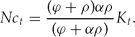
Thus, aggregate consumption at time t 2 is given by the two expressions

Therefore

(iii) Zero expenditures on environmental protection when environmental quality is abundant follows directly from definition 1, and conditions (2) and (5). Additionally, at times larger than t 1 defined in (i), the results from section 2 apply and environmental expenditures, πt, grow at the constant rate ϕ. To see that πt is discontinuous at t 1, notice that πt = 0 for 0 ≤ t<t 1 and  for t ≥ t 1. Therefore

since, by assumption, the term within brackets in the last expression is strictly positive. Furthermore, we can rewrite the last expression as  , where the first equality above follows from (9) and (11) and the last from (13). Thus,
 .
To see that πt is discontinuous at time t 2, use equations (9), (11), and (12) to write

Therefore

Proof of proposition 2
(i) For the policy vector τ = (0, 0)the households' problem is
subject tot = rK t − Nc t, and limt→∞e −ρt νtK t = 0.The first-order conditions give the rate of growth of consumption:
.Firms maximize profits and the resulting rental price of capital is r = A − δ. In equilibrium, the transversality condition and the initial stock of capital yield the equations for consumption per capita
, and capital Kt = K 0e (A−δ−ρ)t.Environmental quality decreases with pollution: Ė t = −PK t. Solving for Et with E 0 given, we have
.The expressions for ct, Kt, and Et are the same as equations (19), (18), and (20).
(ii) See Chimeli (Reference Chimeli2003: 138–140).
(iii) With a non-zero tax on pollution or consumption, the current value Hamiltonian for the households' problem is
and the first-order conditions imply:. We use the conjecture to be verified later that the consumption tax τc is time invariant to obtain . The first-order condition for the profit-maximizing firm gives the competitive price of capital: r = A − δ − τpPThe optimum derived from the social planner's problem is implemented in the decentralized economy if and only if the rate of growth of consumption is identical in both problems and the first-order condition for the firm is satisfied. This implies that the tax on pollution must equal the inverse of marginal environmental protection or the efficiency of environmental protection expenditures:
. That is, the pollution tax equals the units of output spent on an additional unit change of environmental quality per unit of time.Thus, the rental price of capital along the balanced growth path is constant and given by
, and the consumption path, after choosing the initial consumption level according to the social planner's solution is . To obtain the consumption tax τc that implements the economy's first best, we solve for the stock of capital according to the equation of motion for capital:
From the tranversality condition the stock of capital is, implying that the optimal tax on consumption that makes capital identical to the social planner's optimum capital stock in equation (11) is .Tax revenues to be used in the provision of the public good environmental quality are given by tax revenues from consumption plus tax revenues from pollution
as in the first-best level of expenditures on environmental protection in equation (12). Clearly, our conjecture of a time invariant τc works here and environmental quality at time t will follow the same path as in the social planner's solution.(iv) With a non-zero tax on pollution and zero tax on consumption, the household's problem implies that
and the solution to the firm's problem gives r = A − δ − τpP. Thus, consumption will grow at the correct rate if and only if . Therefore, for some constant c 0, the equation of motion for capital becomes , which, along with the tranversality condition, implies that and , for every t such that (7) is binding. These expressions are equations (14)–(16). □

 .
 , and capital Kt = K 0e (A−δ−ρ)t.
 .

 . We use the conjecture to be verified later that the consumption tax τc is time invariant to obtain
 . That is, the pollution tax equals the units of output spent on an additional unit change of environmental quality per unit of time.
 , and the consumption path, after choosing the initial consumption level according to the social planner's solution is

 , implying that the optimal tax on consumption that makes capital identical to the social planner's optimum capital stock in equation (
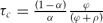 .

 , which, along with the tranversality condition, implies that
 and
 , for every t such that (7) is binding. These expressions are equations (
Proof of corollary 1
To prove this result, it suffices to focus on the balanced growth path of the economy and check whether a tax on profits would be required to implement the Pareto optimal solution. Freely distributed tradable pollution permits are designed to promote the socially optimal level of emissions by firms at each time t, not to generate tax revenues. To obtain the social planner's solution, the government has to tax consumption and profits that may result from the distribution of the permits so as to generate enough tax revenues for the optimal provision of environmental quality.
With this new set of instruments, the households' problem becomes

subject to t = rK t − N(1 + τc)c t + (1 - τη)ηt, where ηt are any profits that the firm generates to households and τηis the tax rate on profits. As before, the same transversality condition applies. As in the tax case, the first-order conditions for the households' problem implies  .
The firm's problem is now

where p is the price of the pollution permit and PK*t is the quantity of permits distributed by the government at time t. The firm's problems under the permit and tax schemes are quite similar. The rental price of capital is r = A − δ −pP, implying that profits are equal to the value of the permits distributed to the firm: ηt = pPK*t. The permit price that implements the optimal solution in a competitive equilibrium is identical to the pollution tax previously analyzed:  . Consequently, the rental price of capital is the same as before
 , and consumption grows at the optimal rate and level with the appropriate initial condition:
 .
The stock of capital at time t is the solution to the law of motion of capital
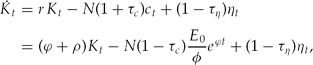
and the optimum can be clearly implemented if the tax on consumption is the same as before and the tax rate on profits is equal to 1, i.e. τη = 1. This way, the equation for capital becomes identical as in the tax scheme, so that Kt = K*t, and tax revenues are  .
In comparison with the pollution tax case, freely distributed pollution permits transfer revenues from the government to firms in the form of profits by the same amount as tax revenues from pollution. To implement the social optimum, the government needs to recover these revenues, and thus has to tax profits by 100%.
If instead of distributing the pollution permits the government decides to sell them to firms at the price p, their problem becomes

which is identical to the pollution tax problem. Thus, the optimum can be implemented with the sales of permits and a consumption tax.
Lastly, if the optimal taxes on pollution and consumption are implemented with an environmental protection function given by Ππβ1tπ1−β2t, the interior solution pollution tax, rental price of capital, and consumption tax are

The results for the freely distributed pollution permits are the same with  η = 1. □