




No CrossRef data available.
EDUCATION VOUCHERS, GROWTH, AND INCOME INEQUALITY
Published online by Cambridge University Press: 01 February 2005
Abstract
This paper studies a growth model with public and private education alternatives. The impact of education vouchers on economic growth and the evolution of income inequality are considered. Results indicate that introducing education vouchers can increase economic growth. Households switching from public to private education experience higher incomes. This raises the tax base, in turn raising public education expenditures and growth of the whole economy. Vouchers are found to generally increase income inequality. Welfare comparisons show that voucher schemes may in some cases gain majority support, depending on assumptions and parameters. The results add a new dimension on which vouchers can be evaluated in the continuing policy debate.
Information
- Type
- ARTICLES
- Information
- Copyright
- © 2005 Cambridge University Press
INTRODUCTION
Reform of education and its financing have been topics of growing importance in policy debates over the past four decades in the United States. Proposals for education vouchers have been increasing in number with numerous pilot programs in place. However, the debate over the beneficiaries of education vouchers continues. Typical issues include the benefits of school choice and competition and the problems of cream skimming the best students and greater inequality to name a few; Cohn (1997) provides a collection of works covering a wide range of issues relevant to education vouchers.
This paper studies the implications of private-education vouchers for economic growth and income inequality. Vouchers take the form of a uniform subsidy to all families using private schools. The policy issue is whether an existing public education budget can be reallocated in a growth-enhancing manner through the use of vouchers. Vouchers raise the incomes of private-education households such that the tax base grows, in turn providing for increased public-education and human capital accumulation for public-education households, a fiscal externality.1
Nechyba (1999) identifies a similar fiscal spillover in a multidistrict model with public and private schools and migration between districts.
The coexistence of public and private education leads to a bimodal income distribution. The effects of vouchers on the dynamic evolution of the economy are studied, though the endogenous distribution of income cannot be analytically characterized. Numerical simulations are used to investigate the implications of vouchers for growth and income inequality. The model is calibrated in accordance with the approach used to study vouchers in a static setting in Epple and Romano (1996), using data on U.S. human wealth distribution estimated by Lillard (1977). An alternative calibration suggested by Cohen-Zada and Justman (2003) is also considered.
The simulation analysis identifies two main results. First, education vouchers increase per capita income and growth. Second, there is indeterminacy with respect to income inequality. Introducing vouchers increases inequality measured using Gini coefficients, though alternative measures identify the possibility of reduced inequality. Generalized Lorenz curves show that vouchers offer Pareto improvement in utilities, though among the early generations to experience vouchers, majorities may be worse off and prefer not to have vouchers in some cases. This is consistent with the U.S. experience that vouchers struggle to gain support in referenda, indicating heavy discounting beyond current generations. The endogenous income distribution is found to exhibit bimodality, with the lower-income group attending public schools and the upper-income group attending private schools. This result has similarities to that of Galor and Zeira (1993). In this case, there is no credit market for human capital, while the additional assumption that leads to multiple equilibria or convergence clubs is that parents must choose between public and private education.2
For a further discussion of dynamic models with multiple equilibria, club convergence, and income distribution, see Galor (1996).
The paper brings together two strands of the literature: first is the study of education vouchers and second is the investigation of links between growth, education, and human capital accumulation. The literature on education vouchers is typically theoretical because of the limited data available for empirical studies, and focuses on one-period models, analyzing the static effects of vouchers on current students.3
One of the few empirical studies of the effects of vouchers is Rouse (1998).
Voucher design and the efficient targeting of education funding are studied by Bearse et al. (2000) and Nechyba (2000). The key results are that (i) vouchers can improve educational outcomes and (ii) appropriately targeting vouchers can provide further improvements in the distribution of educational expenditures and outcomes. Issues of targeting are not studied in this paper in order to simplify the analysis and focus on the positive growth implications of the least beneficial form of vouchers, namely, uniform private-education vouchers.
Another important simplifying assumption is that the existing public education budget is available for reallocation between private-education vouchers and public education for those who do not take up the private alternative while maintaining a balanced government budget. This eliminates voting issues from the model. Although much of the existing literature investigates voting issues, in the overlapping generations framework outlined below, each generation's voting problem would be a self-contained, one-period optimization problem, and the inclusion of social choice will not enrich the model's dynamics or provide new insights into voting issues. Thus, the focus is on dynamic efficiency gains that can be extracted from the existing budget through the simple market mechanism of a uniform private-education voucher.
Education vouchers are studied in a growth setting by Kaganovich and Zilcha (1999). Their work looks at the relationship between social security, education with vouchers, and growth, with the benefits of vouchers for growth depending on parental altruism for their children. Whereas Kaganovich and Zilcha (1999) study a representative-agent framework, this paper considers heterogeneous agents, thereby allowing for the study of income distribution and of dynamic interactions between public- and private-education students. Gradstein and Justman (1997) compare different forms of education finance, namely subsidizing private education and universal private education.4
Other examples of growth models where public and private education alternatives are studied as distinct models include Eckstein and Zilcha (1994), Glomm and Ravikumar (1992), and Gradstein and Justman (2000).
Section 2 sets out the model to be studied. The model is solved and equilibrium is characterized in Section 3. The effects of vouchers on growth and income inequality are studied in Sections 4 and 5, respectively. Numerical simulations are used in Section 6 to further analyze the implications of education vouchers on growth and income inequality. A summary of results is provided in Section 7.
MODEL WITH VOUCHERS
Consider an economy of two-period-lived overlapping generations. The population is normalized to unity and is constant over time, with each parent having only one child. Human capital endowments of the first generation follow some distribution f0(h). For subsequent generations, the human capital distribution is endogenous and given by ft(h) for the cohort that is old in period t+1. Parents (i) inelastically supply their unit time endowment; (ii) are taxed, with revenues used to finance education; and (iii) decide to send their child to a public or private school. If a public school is chosen, all after-tax income is consumed and the child's education is fully government provided. If private education is chosen, an education voucher is available and after-tax income is allocated between private consumption and education.
Parents derive utility from the education provided to their child (qi,t) and household consumption (ci,t), where i and t indices identify, respectively, the agent's type, based on human capital, and the period in which they are old. A constant elasticity of substitution (CES) utility specification is assumed:

where β∈(0, 1), ρ∈(−1, ∞). This preference specification is used by both Epple and Romano (1996) and Cohen-Zada and Justman (2003), and is chosen to facilitate calibration based on these previous studies.
A child's human capital depends on the education expenditure made on his or her behalf and on the parents' human capital. Human capital (hi,t) evolves according to

where γ∈(0, 1) and θ>0. Individual human capital accumulation depends on education expenditures and levels of parental education.
Parents inelastically supply their unit time endowment at a wage given by their human capital, with income (yi,t) given by

This assumption allows a clear focus on the implications of education expenditure and choices, exclusive of labor supply decisions, on income distribution.
Two schooling alternatives are available: public or private. In the public-education system, students receive identical, government-funded education expenditures. The parent does not make any other contributions. If public education is chosen, the parent's education expenditure and budget constraint are, respectively, given by


where τ is the marginal tax rate imposed on all income. Since the model abstracts from voting issues, the tax rate is treated as exogenous and does not vary over time. Tax revenue is used solely to finance education, either public education or private-education vouchers.
The proportion of the population in public education in period t is given by Qt∈(0, 1) while per student public-education expenditure is given by

where Yt is both aggregate and average income and (1−Qt) is the proportion of the population receiving private education. The voucher provided to parents choosing private education is given by

where s is the size of the voucher as a fraction of average income, hereafter the subsidy rate. It is assumed that the subsidy rate is sufficiently small that Et>St. This link between vouchers and per capita income is a simplifying assumption. Various forms of private-education subsidies are used around the world, in Australia, France, and the Netherlands to name a few. Costs and the behavior of subsidies depend on the educational structure. In the Netherlands, for example, average costs are increasing because of the proliferation in the number of smaller private schools; see Cohn (1997) and West (1997) for more details.
If the parent opts out of the public system, the child's education is financed out of after-tax income, which is supplemented by a private-education voucher, St. This voucher can only be used at private schools and cannot be used to purchase consumption, implying that if private education is chosen, qi,t>St.5
The corner solution qi,t=St cannot be an equilibrium because of the assumption that Et>St, so that a household considering the corner solution would always prefer public education with qi,t=Et.


where ei,t is the private-education spending by the parent; this is similar to the voucher framework used by Epple and Romano (1996).
The tax and the subsidy rates are determined by the government, and individual agents treat them both as exogenous. The issue of interest here is whether a shift from an education system where s=0 to a system where s>0, while maintaining τ constant, can increase growth and reduce income inequality. The determination of either the tax or subsidy rates could be endogenized using majority voting, as in Epple and Romano (1996) and Glomm and Ravikumar (1999). Alternatively, both the tax and subsidy rates could be determined endogenously in a sequential voting framework as in Hoyt and Lee (1998). The lack of strategic interaction between cohorts or generations means that each generation's voting problem would be a distinct static political optimization problem, the inclusion of which complicates the analysis and does not enrich the dynamics of the model.6
Developing the model in such a way that incorporating voting leads to strategic interaction between cohorts is the subject of ongoing research but is beyond the scope of the present study.
EQUILIBRIUM PROPERTIES WITH VOUCHERS
A general equilibrium for the model described by equations (1) to (9) comprises a set of sequences of individual choices for consumption and education, {ci,t, qi,t}∞t=1, that maximize individual utility, given the tax and subsidy rates (τ, s). Equilibrium also requires that, at the given tax and subsidy rates (τ, s) and per capita income {Yt}∞t=1, the public education expenditure and enrollment, {Et, Qt}∞t=1, are such that the government budget balances, satisfying (6).
Optimal choices of a parent who sends his or her child to public school are


The dynamic evolution of human capital for a public-education family is given by

which can be solved for a state-dependent fixed point,

This fixed point depends on aggregate state variables Yt and Qt and on the exogenous, government-determined tax and subsidy rates, τ and s. The human capital of all students sent to public school in periodt will converge to hf,u t, though at different rates depending on their parents' human capital, hi,t−1. This fixed point may change in the subsequent period because both Yt+1 and Qt+1 may differ from their period t values; hence, hf,u t cannot strictly be referred to as a steady state.
The optimal choices of a parent choosing private education for his or her child are given by


where B=[β/(1−β)]1/(1+ρ). Private education can be an optimal choice for a parent only if

which ensures that qi,t>St, a necessary condition for the optimality of the choice of private education, given that consumption cannot be purchased with vouchers and Et>St.
Human capital evolves according to the following dynamic equation in the private-education model:

This dynamic equation provides some restrictions on parameters to be used in the simulation analysis. When s=0, the dynamic equation is linear in hi,t−1 and the coefficient, θ[(1−τ)/(1+B)]γ, must be greater than unity to rule out trivial equilibria. When s>0, equation (17) is strictly concave, but it is not sufficiently concave for a fixed point to exist.7
Deriving a fixed point for equation (17) yields

If we impose the assumption that θ[(1−τ)/(1+B)]γ>1, then hf,r t<0, which makes no economic sense and is not considered further.
PROPOSITION 1. In equilibrium, assuming that θ[(1−τ)/(1+B)]γ>1 and s>0, the dynamic equation for private-education human capital satisfies the following conditions:
- and
- .
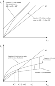
The proof can be found in Cardak (2001). Thus, no private-education fixed point for human capital exists. The expansion path is not linear as in an AK growth model, but is instead concave, whereas in the limit, as hi,t−1 → ∞, it is weakly concave or approaches linearity. This behavior is illustrated in the top panel of Figure 1.

Dynamics of human capital given by equations (12), (13), and (17). The top panel shows private education case and bottom panel shows public education case. The bottom panel also shows the effects of the voucher-generated fiscal spillover on public education (after k periods), raising the growth path.
Each parent chooses the education system that provides greatest utility. This in turn depends on own income, the sizes of the tax and voucher rates, public school enrollment, and per capita income, all of which determine the relative attractiveness of public and private education. To find an income threshold that separates the population into public- and private-education groups, substitute equations (10) and (11) into (1), and (14) and (15) into (1); equate and solve for the level of income at which parents are indifferent between alternatives, y*t. Though y*t cannot be explicitly characterized, the following result ensures its existence and uniqueness.
PROPOSITION 2. For a given tax and voucher rate, τ and s, public education expenditure, Et, and per capita income, Yt, there exists a unique income threshold y*t=y(Et, Yt; τ, s) such that all parents with yi,t[les ]y*t prefer public education and those parents with yi,t>y*t prefer private education.
The proof can be found in Cardak (2004a). The result means that the poor will prefer public education and the rich will prefer private education. It allows the proportion of the population in public education, Qt, to be uniquely determined for a given combination of (Et, Yt; τ, s):

where Ft−1(·) is the c.d.f. and ft−1(·) is the p.d.f. of human capital accumulated in period t−1. Alternatively, Qt can be determined from equation (6).
VOUCHERS AND GROWTH
The potential gains from the introduction of a private-education voucher in this model can be illustrated with a simplified example. Consider an economy with three groups of homogeneous agents: the poor, the middle class, and the rich, respectively, comprising fractions Q1, Q2, and (1−Q1−Q2) of the population, with respective incomes y1,t, y2,t, and y3,t such that y1,t<y2,t<y3,t. The poor and middle class attend public schools, while the rich attend private schools. In terms of y*t from Proposition 2, y1,t and y2,t[les ]y*t=y[Yt, Qt=(Q1+Q2); τ, s=0]<y3,t.
Consider the introduction of a private-education voucher St=sYt, which causes only the middle class, Q2, to switch to private education. The rich and middle class receive the voucher and attend private schools while the poor continue to attend public schools. It is now the case that y1,t[les ]y*t=y(Yt, Qt=Q1; τ, s)<y2,t and y3,t.8
This assumption has implications for the value of s. Recall that the value of y*t comes from an indifference between the use of the public or private education alternatives; see Proposition 2 and its proof. Since, in this case, y1,t, y2,t, and y3,t are given, s must be chosen so that the assumption holds. Although y1,t[les ]y*t and y*t<y2,t, respectively, place upper and lower bounds on s, these bounds can only be characterized implicitly because of the utility function assumed in equation (1).
Using equation (12) for public education and equation (17) for private education, the first generation of rich students to use the voucher are better off:

where the superscript V and NV denote cases with and without vouchers, respectively. The value of s is chosen so that middle-class parents are better off. Middle-class students will have higher human capital if

which places the following lower bound on s:

For poor students, public-education expenditures will benefit from the reduction in public school enrollments from (Q1+Q2) to Q1, but the public education budget will be reduced because of voucher expenditure. Poor students will have higher human capital under the voucher scheme if

which occurs only if

This condition requires the voucher scheme to raise per student public education expenditures, Et, and occurs when the costs of the voucher program (LHS) are lower than the benefits of vouchers (RHS) in terms of the public education budget.9
In addition to the conditions outlined in note 8, equations (16) and (23) identify an upper bound for s while equation (21) provides a lower bound. Together, these conditions define, for this example, the feasible space for s. This space cannot be analytically simplified to explicit lower and upper bounds; however, the simulations employed below confirm the non-emptiness of this space.
If the voucher is too small, however, the middle class may not be induced out of the public education system and the gains will not be achieved.
If all households have higher human capital after the introduction of vouchers, per capita income in the next period must be higher, which will provide further growth to subsequent generations of poor students, through a tax-base-driven improvement in public education, a fiscal spillover. It is not clear whether all households benefit in the long run if the human capital of poor students is initially lowered by vouchers. This will occur if the voucher is large, leaving few resources for public education, hurting the poor group, and benefiting the upper- and middle-income groups. In the longer run, whether the fiscal spillover operates to increase human capital for the poor is investigated using the simulations below.11
Bénabou (1996) uses a richer model with local and global linkages. Although the voucher studied here reduces within-group inequality, it has the potential to widen the gap between groups. In a model such as Bénabou's, with economywide production complementarities, the resource reallocation of a voucher could lead to lower growth outcomes, depending on the relative importance of local and global interactions and the change in the distribution of human capital.
VOUCHERS AND INCOME INEQUALITY
Endogenous income distribution cannot be analytically characterized in this model because of the discrete education choices. Parts of the income distribution are characterized below using within-group comparisons; this is later supplemented with simulations.
Focusing on households that attend public schools whether private-education vouchers are available or not, the relevant dynamic equation is (12). Comparing two families, j and k, in this group, the ratio of their incomes is

Incomes within this group converge over time, as γ∈(0, 1). Introducing private-education vouchers will not change the rate at which incomes converge among those who continue to use public education because vouchers change public education identically for all public-education students. This changes income levels by a constant scale factor, leaving relative inequality within this group unchanged.
The relevant dynamic equation for households that use private education both before and after the introduction of vouchers is (17). Comparing families l and m from this group, the income ratio is

In the case without vouchers, s=0, relative inequality within this group does not change over time.
Introducing private-education vouchers leads incomes within this group to converge over time. Assuming hl,t−1>hm,t−1, changing the subsidy rate from s=0 to s>0 reduces the income of household l relative to household m from period t−1 to period t:

This result arises because vouchers reduce the relative differences in education expenditures within this group of private-education users.
The effects of vouchers on mobile groups (switching from public to private education) has not been considered because the endogenous income distribution cannot be fully characterized. Simulations are used in the next section to further characterize the impact of vouchers.
DYNAMIC ANALYSIS
Calibration
The model is calibrated to match aggregate variables and behavior observed in the United States, following the methodology of Epple and Romano (1996). Simulations are used to illustrate the endogenous distribution of income for cases with and without vouchers. The approach is to simulate the model for a large sample and use the income distribution of the sample as an approximation to the actual endogenous income distribution. Economic variables are plotted over time to illustrate the differences between the cases with and without vouchers.
Since the model is of overlapping generations and yi,t=hi,t, the first generation's income distribution is calibrated to human wealth distribution in the United States, as suggested by Glomm and Ravikumar (1999). The figures used are based on Lillard's (1977) estimation of human wealth distributions in 1970, where mean and median human wealth (measured in thousands) are, respectively, $166.99 and $151.39. These figures are adjusted to 1996 prices using the Consumer Price Index (CPI), with a mean of $515.04 and median of $466.93. Assuming lognormality implies that ln(hi,0)∼N(μ, σ2), with μ=6.146 and σ=0.443, where hi,0 are the human capital endowments of the first generation.
Public education expenditure in 1996–1997 was $5,882 per student. To be consistent with the human wealth calibration above, the cost of 12 years of education is treated as education expenditure. Thus, per household public-education expenditures are set to $35,292 for the first generation. This assumes approximately 0.5 student per household; see Epple and Romano (1996) and Bearse et al. (2000). The tax rate is chosen to finance the education budget and maintained at this rate for the full time horizon of the simulations. The model parameters β and ρ are chosen so that the model endogenously allocates 12% of enrollments to private education in the first period, as observed in the United States in 1996–1997. These data are drawn from Public Elementary-Secondary Education Finance Data: 1996–1997, US Bureau of the Census (2000) and the Digest of Education Statistics 1999, National Center for Education Statistics (2000).
Two combinations of preference parameters (ρ, β) are used to investigate the model. The first (Case A) is the benchmark case used by Epple and Romano (1996), where ρ=0.54 and β=0.967, which leads to private-education enrollments of 12% and implies an elasticity of substitution of −0.65. The second case (Case B), where ρ=−0.359 and β=0.750, also provides private-education enrollments of 12% with an elasticity of substitution of −1.56. This parameterization is suggested by Cohen-Zada and Justman (2003), who present a unified theory-estimation-calibration-simulation approach to a similar one-period model.12
They assume that private education is more efficient at providing education services, which leads to a higher value for β=0.846 in order to match U.S. private enrollment data. Given that it is assumed here that public and private education are equally efficient, a value of β=0.750 results in enrollments matching U.S. data and is used in the simulations where ρ=−0.359.
In the calibration of the human capital production function, θ is chosen so that θ[(1−τ)/(1+B)]γ>1, as discussed in Section 3, and that aggregate growth is around 2% per year. Assuming that a generation comprises 30 years, this amounts to 81% growth per period. Although a precise value for γ is difficult to pin down and is open to debate, empirical studies suggest that γ<0.5. Glomm and Ravikumar (1998) simulate a model with a similar human capital production function and assume γ∈(0, 0.15). The results reported here focus on the case in which γ=0.1, while sensitivity analysis of the results includes the cases in which γ=0.01 and 0.2. The sample size used to approximate the distribution of income is chosen to be 10,000 while the model is simulated for 50 generations. Details of the simulation process are contained in Cardak (2001).
Results
Three vouchers are considered, with S0=$0, $12,000, $24,000 (for 12 years of schooling). These absolute voucher values are allowed to grow over time, while maintained as a constant proportion of average human wealth. In Figures 2 and 3 below, Case A is considered, ρ=0.54, β=0.967, θ=2.33, γ=0.1, while in Figures 4 and 5, Case B is considered, ρ=−0.359, β=0.750, θ=2.304, γ=0.1.

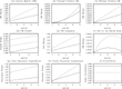
Time series of (a) per-capita, (b) poorest family's, and (c) richest family's human wealth; (d) growth rates for per capita human wealth; human wealth inequality measured by (e) the Gini coefficient; and by (f) ratios of ninth- to first-decile income; (g) education expenditure, including all vouchers; (h) per student public education expenditure; and (i) public education enrollments. Ratios of the voucher cases to the no voucher case in panels (a)–(c) and (e)–(h), with S0=$12,000 (solid curve) and S0=$24,000 (dashed curve). In panels (d) and (i), plots are for the cases S0=$0 (solid curve), S0=$12,000 (dashed curve), and S0=$24,000 (short dashed curve). Parameter values for Case A are θ=2.33, γ=0.1, ρ=0.54, and β=0.967.

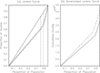
(a) Lorenz curves, and(b) generalized Lorenz curves, for income distributions with novouchers, S0=$0 (solid curves), and with vouchers, S0=$24,000 (dashed curves), after five generations. Parameter values for Case A, θ=2.33, γ=0.1, ρ=0.54, β=0.967.

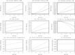
Time series of (a) per capita, (b) poorest family's, and (c) richest family's human wealth; (d) growth rates for per capita human wealth; human wealth inequality, measured by (e) the Gini coefficient, and by ratios of (f) ninth- to first-decile income; (g) education expenditure, including all vouchers; (h) per student public education expenditure; and (i) public education enrollments. Ratios of the voucher cases to the no-voucher case in panels (a) to (c) and (e) to (h), with S0=$12,000 (solid curve) and S0=$24,000 (dashed curve). In panels (d) and (i), plots are for the cases S0=$0 (solid curve), S0=$12,000 (dashed curve), and S0=$24,000 (short dashed curve). Parameter values for Case B are θ=2.304, γ=0.1, ρ=−{0.359}, and β=0.750.

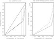
(a) Lorenz curves and(b) generalized Lorenz curves for income distributions with novouchers, S0=$0 (solid curves), and with vouchers, S0=$24,000 (dashed curves), after five generations. Parameter values for Case B, θ=2.304, γ=0.1, ρ= −0.359, β=0.750.
Case A
Human wealth and growth
Vouchers raise per capita human wealth for Case A, see panel (a) of Figure 2, which shows ratios of per capita human wealth with vouchers to per capita human wealth without vouchers for vouchers of S0=$12,000 (solid curve) and S0=$24,000 (dashed curve). Private education vouchers will immediately raise average human wealth. After five generations, average human wealth can be 3.2% higher if S0=$24,000.
The ratios of the poorest and richest family's human wealth with vouchers to human wealth without vouchers for S0=$12,000 (solid curve) and S0=$24,000 (dashed curve) are presented in panels (b) and (c) of Figure 2, respectively. The poorest family always has higher human wealth with vouchers. The increase in human wealth is initially smaller with the larger voucher. This is due to initial reductions in public education expenditure. Panel (c) of Figure 2 indicates that the wealthiest family always has higher human wealth with vouchers than without. This identifies the poor as being among the beneficiaries from private-education vouchers. These gains arise from endogenous increases in public-education expenditure.
Annual growth rates for per capita human wealth are presented in panel (d) of Figure 2 for S0=$0 (solid curve), S0=$12,000 (dashed curve), and S0=$24,000 (short dashed curve). Growth rates are up to 0.9% higher with vouchers (when S0=$24,000). This results from the larger number of private-education families, providing a greater tax base and enhancing the fiscal spillover that drives the endogenous growth of the public education sector.
Income distribution, inequality, and welfare
Panel (e) of Figure 2 shows ratios of Gini coefficients with vouchers to Gini coefficients without vouchers for S0=$12,000 (solid curve) and S0=$24,000 (dashed curve). Vouchers increase human wealth inequality measured by Gini coefficients. After five generations, Gini coefficients are up to 5.5% higher with vouchers than without. Inequality increases because families switching from public to private education are moving further into the upper tail of the human wealth distribution, moving further above the mean and raising overall human wealth inequality.
Human wealth inequality is also measured by the ratios of voucher to no-voucher cases of the ninth- to the first-decile human wealth ratio and is plotted in panel (f) of Figure 2 for S0=$12,000 (solid curve) and S0=$24,000 (dashed curve). The ninth- to first-decile ratios suggest vouchers lead to very little change in human wealth inequality. This implies that although vouchers may increase Gini coefficients, panel (e), the extrema of the distribution are largely unaffected. The main changes in the distribution are between the 82nd and 88th percentiles, those switching education regimes.
Further exploring inequality, Lorenz and generalized Lorenz curves (GLC's) for the distribution of human wealth after five generations are presented in panels (a) and (b) of Figure 3, with S0=$0 represented by the solid curve and S0=$24,000 represented by the dashed curve. The Lorenz curve in panel (a) is divided into three regions: (i) below the vertical line at 0.82 are those households that attend public schools with and without vouchers; (ii) between 0.82 and 0.88 are the households that use public schools without a voucher and private schools with a voucher, the mobile families; and (iii) above the vertical line at 0.88 are those households who always attend private schools. This Lorenz curve confirms the analytical result that relative inequality within the public-education group does not change with the introduction of vouchers [equation (24)]. This can be seen by the linear portion of the Lorenz curve, which measures inequality within the public-education group.13
Linearity of a portion of a Lorenz curve implies perfect equality within that subgroup.
The GLC's in panel (b) have welfare implications. Because the GLC for the case with S0=$24,000 lies above the GLC for the case with S0=$0, the human wealth distribution with vouchers stochastically dominates the distribution without vouchers. The case in which S0=$12,000 is not presented but the GLC lies entirely between the GLC's for the no-voucher and S0=$24,000 cases. This implies that all agents are better off with vouchers in terms of utility; thus, after five generations, vouchers offer a welfare improvement.
This raises the question of how long it takes for vouchers to gain majority support. Individual utilities under the two alternative voucher values are calculated and compared to the case with no vouchers. Comparisons indicate that a voucher policy with S0=$12,000 gains immediate majority support whereas a voucher policy with S0=$24,000 gains majority support by the third generation. The results for the larger voucher are consistent with the fact that in the United States, referenda proposing the introduction of vouchers repeatedly fail to attract majority support.
Human wealth distribution in the mixed-education model, both with and without vouchers, is bimodal.14
See Cardak (2004b) for an example of this without vouchers.
Education spending and enrollment
Ratios of total per student education expenditures with vouchers to per student education expenditures without vouchers are presented in panel (g) of Figure 2 for the cases of S0=$12,000 (solid curve) and S0=$24,000 (dashed curve); the same ratios for per student public education expenditures are presented in panel (h) of Figure 2. Private-education vouchers immediately increase total education expenditures. After five generations the total education budget is 4% higher in the case in which S0=$12,000 and 8.5% higher in the case in which S0=$24,000. Panel (h) shows that per student public education expenditures initially suffer from the introduction of vouchers. In the case in which S0=$24,000, they are 2% lower than in the no-voucher case, but after three generations, the increase in the tax base has raised per student public education expenditures, and after five generations, public education expenditures are 4% higher than they would have been without a voucher.
The higher total education expenditure in panel (g) is the key source of the increased growth after the introduction of private education vouchers. Higher education spending results from two factors: First is the initial increase in total private-education spending due to the voucher shifting more people into private education. Although average private-education expenditure decreases, the larger numbers in private education raise total education expenditure.15
In the case with vouchers, the same goverment budget is expended on education while the families that switch to private education spend more on education as do those that were already in private education.
In panel (i) of Figure 2, the proportion of the population in public education is presented for the case of no vouchers or S0=$0 (solid curve), S0=$12,000 (dashed curve), and S0=$24,000 (short dashed curve). Larger vouchers entice larger numbers of people out of the public education system, with the lowest public education enrollments in the case of S0=$24,000. The S0=$24,000 voucher reduces public school enrollment from 88% in the case without a voucher to 81.8%. These changes in enrollment are larger than those found in Epple and Romano (1996) because taxes are held fixed at the rate required to balance the public education budget in the case without vouchers. Once vouchers are introduced, the government budget is still required to balance but taxes do not rise, making private education more attractive (or relatively cheaper) and drawing more students into private education than observed by Epple and Romano (1996).16
The key reason for this difference is that Epple and Romano (1996) endogenize the tax rate, since their primary interest is in their theoretical voting equilibrium results established earlier in their paper.
Case B
Case B assumes ρ=−{0.359}, β=0.750, θ=2.304, γ=0.1 . For Case B, intergenerational altruism is higher because the elasticity of substitution between education and consumption is higher and the weight on the consumption good is smaller. Hence, education is more important to parents who are more willing to substitute education for consumption, relative to Case A. Analysis of Case B is presented in Figures 4 and 5, and closely follows that of Case A.
Per capita income and growth
Panel (a) of Figure 4 shows the effects of vouchers on per capita human wealth for Case B, illustrating that vouchers immediately offer increased per capita human wealth in Case B. The impact on per capita human wealth is larger than in Case A and, after five generations, per capita income is 3.5% higher when S0=$12,000 and 7% higher when S0=$24,000.
Panel (b) of Figure 4 shows that for Case B, the poorest family's human wealth is higher with vouchers than without vouchers. After five generations, the poorest family's human wealth is increased by 0.78% when S0=$12,000 and by 1.5% when S0=$24,000. Panel (c) of Figure 4 shows the richest family's human wealth is always higher with vouchers, by 0.08% when S0=$12,000 and by 0.16% when S0=$24,000. The poor benefit more from vouchers in Case B because the elasticity of public enrollments with respect to vouchers is higher than in Case A; this is discussed further below.
Growth rates for Case B are presented in panel (d) of Figure 4 and show the initial increase in growth to be greater than in Case A. When S0=$24,000, the initial growth rate is 2.40% higher than for the case without vouchers, while for S0=$12,000 the initial growth rate is 1.2% higher. After five generations, these differentials are 2.2% and 1.1%, respectively.
Income distribution, inequality, and welfare
The ratios of Gini coefficients are presented in panel (e) of Figure 4. As in Case A, vouchers raise the Gini coefficient, initially by 1.2% for S0=$12,000 and 2.3% for S0=$24,000. After five generations, Gini coefficients are 4.3% and 8.2% higher for the respective vouchers.17
In the very long run, after 50 generations, the inequality results do appear a little different, with vouchers able to reduce inequality. These results are not presented here because of space constraints and the fact that 50 generations equates to 1,500 years, a time horizon of relatively limited policy interest; details can be found in Cardak (2001) or on request from the author.
The ratios of voucher to no-voucher cases of the ninth- to the first-decile income ratio are plotted in panel (f) of Figure 4. These ratios show, as in Case A, very little change due to vouchers. In contrast to Case A, these ratios fall with the introduction of vouchers, and the larger voucher, S0=$24,000, reduces inequality by more than the smaller voucher, implying that for Case B, the extrema of the distribution are brought closer together by vouchers.
The Lorenz and GLC's for the distribution of income after five generations for Case B are presented in panels (a) and (b) of Figure 5. The Lorenz curves show that the voucher increases the share of total income of families that switch from public to private education, primarily at the cost of the wealthy (those who were in private education without vouchers), whereas those that remain in public education suffer only small reductions in their share of total income. The Lorenz curves with and without vouchers cross, implying that alternative measures of inequality that contradict the Gini coefficient can be found, consistent with results in panel (f) of Figure 2; see Atkinson (1970) for a detailed discussion.
The GLC's in panel (b) imply that the distribution of human wealth when S0=$24,000 stochastically dominates the human wealth distribution when S0=$0. Thus, after five generations for Case B, all agents are better off with vouchers, a unanimous welfare improvement.
Comparing individual utilities under the no-voucher case with the two alternative voucher values, it is again found that vouchers obtain immediate majority (unanimous) support for both S0=$12,000 and S0=$24,000. Typically, political support for voucher schemes has been weak, contradicting these results. One possible explanation is that in the model, all households have school-age children, thereby ignoring issues of the actual demographic profile of the voting population.
Human wealth distributions for Case B are bimodal, as in Case A. The extrema of these distributions are closer together [panel (f) of Figure 4], implying lower inequality with larger vouchers. Examples of these distributions can be found in Cardak (2001).
Education spending and enrollment
The ratios of total per student education expenditures with vouchers to per student education expenditures without vouchers are presented in panel (g) of Figure 4 while the same ratios for per student public education expenditures are presented in panel (h) of Figure 4. The differences in education expenditures for Cases A and B explain the differences in growth and income inequality in the two cases.
Panel (g) of Figure 4 shows that vouchers immediately raise total education expenditures as in Case A, but by greater amounts, by 6.4% where S0=$12,000 and 14% where S0=$24,000. After five generations, education expenditures are up to 9.4% higher for S0=$12,000 and 20.5% higher for S0=$24,000.
Panel (h) shows that for Case B, both vouchers raise per student public education expenditures for every generation. Initially, the increase is 1.2% for S0=$12,000 and 2.0% for S0=$2,000; after five generations the increases are 4.0% and 8.0%, respectively. The public education system experiences a greater benefit from the introduction of vouchers in Case B than in Case A.
Public education enrollments are illustrated in panel (i) of Figure 4. Enrollments are more responsive to vouchers in Case B; more households switch from public to private education for a given voucher. Public enrollments fall by 4.1% for S0=$12,000, by 9.8% for S0=$24,000; the declines are 3.0% and 7.1%, respectively, for Case A. The larger this elasticity of public enrollments with respect to vouchers is, the smaller the reduction in public education expenditures per student because the more students that switch, the fewer public education students among whom the residual public education budget has to be shared. Thus, in Case B, public education expenditure is higher with the introduction of vouchers, leading to higher incomes, explaining the results in panels (a) through (d) of Figure 4.
Sensitivity Analysis
Production Parameters
Cases A and B are analyzed using the alternative values of γ=0.01 and γ=0.2. The results are qualitatively similar to those for Cases A and B considered earlier, with γ=0.1. The main difference is that the increased growth from the introduction of vouchers is lower in the case where γ=0.01 and higher in the case where γ=0.2. This is to be expected because a smaller (larger) value for γ reduces (increases) the importance of education expenditure in human capital production. Vouchers will generate smaller spillovers and will be less beneficial for growth if education spending is less important in the accumulation of human capital. This shows up in both Cases A and B in higher (lower) human wealth and education expenditure when γ=0.2 (γ=0.01). Inequality is largely unchanged except that the 9th- to 10th-decile ratios in both cases with γ=0.2 show reduced inequality, again consistent with the increased growth arising from vouchers. Welfare comparisons indicate that Case B is not sensitive to changes in γ and vouchers continue to receive unanimous support. For Case A, increasing γ to 0.2 provides greater support for vouchers, whereas reducing γ to 0.01 reduces support for vouchers with S0=$ 24,000 not supported by a majority until the eighth generation.
Preference Parameters
Two additional combinations of preference parameters (ρ, β) are considered, with ρ=1.00 and β=0.991 (θ=2.34, γ=0.1) and substitution elasticity of −0.50, and ρ=−0.70 and β=0.59 (θ=2.275, γ=0.1) with a substitution elasticity of −3.33. In both cases, private-education enrollments are 12%. The results are again qualitatively similar to those for Cases A and B; however, the size of the impact of vouchers on growth does depend on the elasticity of substitution. When ρ=−0.70 (1.00), the impact of vouchers on growth is stronger (weaker), relative to Cases A and B. This shows up in higher public and total education expenditures when ρ=−0.70. This difference arises from the increased substitutability between education and consumption with ρ=−0.70, leading to higher education expenditures, human capital growth, and spillovers arising from vouchers. In Cases A and B, vouchers increase Gini coefficients; this is unchanged for the alternatives considered here: Gini coefficients are higher (lower) than in Cases A and B when ρ=−0.70 (1.00). Conversely, vouchers reduce (increase) 9th- to 1st-decile human wealth ratios relative to Cases A and B when ρ=−0.70 (1.00). Welfare comparisons for the case in which ρ=−0.70 and β=0.59 indicate unanimous support for vouchers, as in Case B. For the case in which ρ=1.00 and β=0.991, both the large and small vouchers receive majority support only from the fourth generation onward.
CONCLUSIONS
Increased economic growth has been largely ignored as a potential benefit of education vouchers. In a setting where households can opt out of public education in preference for private education, private-education vouchers have been shown to offer increased economic growth. Taxes were held constant and it was shown that a given public education budget can be redistributed through the use of private- education vouchers in a way that will increase per capita human wealth and in some cases increase the human wealth of all households.
Private-education vouchers generated increased economic growth through a fiscal spillover. The tax base grew through a redistribution of the wealthier public-education students into the private education system where they accumulated greater amounts of human capital. This drove increases in public education expenditure, generating growth for the students remaining in public education. Similar growth enhancement might be generated by ability-tracking or selective-entry schools; however, such systems require some decision rule on how to select students. Vouchers offer an endogenous market mechanism through which these results might be generated. Enriching the dynamic model studied here with heterogeneous abilities and recursive preferences might shed light on whether a voucher system would be more efficient at enhancing growth than a system of ability tracking. This is reserved for future research.
Although it was found in some cases that the introduction of vouchers unanimously increased utility, this was not always the case. The first generation might be averse to private-education vouchers because they may reduce current public education spending, only delivering public-education improvements to subsequent generations. One possible way by which this aversion might be diminished is to means test voucher entitlements. This was found by Bearse et al. (2000) to generate greater political support for vouchers in a static setting.
The model abstracted from the issues of between-school competition and peer effects, important factors in the voucher debate. Incorporating competition for students with vouchers is argued to generate better educational outcomes for students in both private and public schools. This would increase growth in both the public and private education systems, strengthening the increased growth identified here.
Extending the model to incorporate peer effects may be perceived to weaken or overturn the results. This is not necessarily the case. Although the best or most able peers are most likely to leave public schools because of the introduction of a private-education voucher, as in Epple and Romano (1998), growth prospects would improve in the private education system and be harmed in the public system. In a peer-effect growth setting, the operative mechanism in this paper, the fiscal spillover that improves public education, would be strengthened and the voucher should provide better public education and enhance the growth of the whole economy. However, the public-education group may suffer larger losses in the early stages of a voucher program, as they lose their best peers along with public education funds. In addition, inequality is likely to increase more than identified here, at least in the short run. This is an obvious direction for further research on the implications of vouchers for growth.
I am grateful for comments and suggestions from Oded Galor, Gerhard Glomm, Omer Moav, Richard Romano, Joseph Zeira, and seminar participants at Australian National University and Ben Gurion, Hebrew, and La Trobe Universities. I am also grateful for comments and suggestions from two anonymous referees and an anonymous associate editor.
References
Atkinson A.B.
1970
On the measurement of inequality.
Journal of Economic Theory
2,
244–
263.Google Scholar
Bearse P.,
G. Glomm &
B. Ravikumar
2000
On the political economy of means-tested education vouchers.
European Economic Review
44,
904–
915.Google Scholar
Bénabou R.
1996
Heterogeneity, stratification, and growth: Macroeconomic implications of community structure and school finance.
American Economic Review
86,
584–
609.Google Scholar
Card D. &
A.B. Krueger
1992
Does school quality matter? Returns to education and the characteristics of public schools in the United States.
Journal of Political Economy
100,
1–
40.Google Scholar
Cardak B.A.
2001
Education Vouchers, Growth and Income Inequality.
School of Business discussion paper A01 06,
La Trobe University.
Cardak B.A.
2004a
Education Vouchers, Growth and Income Inequality.
School of Business discussion paper A04 03,
La Trobe University.
Cardak B.A.
2004b
Education choice, endogenous growth and income distribution.
Economica
71,
57–
81.Google Scholar
Cohen-Zada D. &
M. Justman
2003
The political economy of school choice: Linking theory and evidence.
Journal of Urban Economics
54,
277–
308.Google Scholar
Cohn E.
1997
Market Approaches to Education: Vouchers and School Choice.
Oxford, New York, and Tokyo:
Elsevier Science, Pergamon.
Eckstein Z. &
I. Zilcha
1994
The effects of compulsory schooling on growth, income distribution and welfare.
Journal of Public Economics
54,
339–
359.Google Scholar
Epple D. &
R.E. Romano
1996
Ends against the middle: Determining public service provision when there are private alternatives.
Journal of Public Economics
62,
297–
325.Google Scholar
Epple D. &
R. Romano
1998
Competition between private and public schools, vouchers and peer group effects.
American Economic Review
88,
33–
62.Google Scholar
Galor O.
1996
Convergence? Inferences from theoretical models.
Economic Journal
106,
1056–
1069.Google Scholar
Galor O. &
J. Zeira
1993
Income distribution and macroeconomics.
Review of Economic Studies
60,
35–
52.Google Scholar
Glomm G. &
B. Ravikumar
1992
Public versus private investment in human capital: Endogenous growth and income inequality.
Journal of Political Economy
100,
818–
834.Google Scholar
Glomm G. and
B. Ravikumar
1998
Flat-rate taxes, government spending on education, and growth.
Review of Economic Dynamics
1,
306–
325.Google Scholar
Glomm G. &
B. Ravikumar
1999
Vouchers, Public and Private Education, and Income Distribution.
Mimeo, University of Iowa.
Gradstein M. &
M. Justman
1997
Democratic choice of an education system: Implications for growth and income distribution.
Journal of Economic Growth
2,
169–
183.Google Scholar
Gradstein M. &
M. Justman
2000
Human capital, social capital and public schooling.
European Economic Review
44,
879–
890.Google Scholar
Hoyt W.H. &
K. Lee
1998
Educational vouchers, welfare effects, and voting.
Journal of Public Economics
69,
211–
228.Google Scholar
Kaganovich M. &
I. Zilcha
1999
Education, social security and growth.
Journal of Public Economics
71,
289–
309.Google Scholar
Lillard L.A.
1977
Inequality: Earnings vs. human wealth.
American Economic Review
67,
42–
53.Google Scholar
National Center for Education Statistics
2000
Digest of Education Statistics, 1999.
http://nces.ed.gov/pubs2000/digest99/.
Nechyba T.J.
1999
School finance induced migration and stratification patterns: The impact of private school vouchers.
Journal of Public Economic Theory
1,
5–
51.Google Scholar
Nechyba T.J.
2000
Mobility, targeting and private school vouchers.
American Economic Review
90,
130–
146.Google Scholar
Rouse C.E.
1998
Private school vouchers and student achievement: An evaluation of the milwaukee Parental Choice Program.
Quarterly Journal of Economics
113,
553–
602.Google Scholar
U.S. Bureau of the Census
2000
Public Elementary-Secondary Education Finance Data: 1996–97.
http://www.census.gov:80/govs/www/school.html.
West E.G.
1997
Education vouchers in principle and practice: A survey.
World Bank Research Observer
12,
83–
103.Google Scholar
Dynamics of human capital given by equations (12), (13), and (17). The top panel shows private education case and bottom panel shows public education case. The bottom panel also shows the effects of the voucher-generated fiscal spillover on public education (after k periods), raising the growth path.
Time series of (a) per-capita, (b) poorest family's, and (c) richest family's human wealth; (d) growth rates for per capita human wealth; human wealth inequality measured by (e) the Gini coefficient; and by (f) ratios of ninth- to first-decile income; (g) education expenditure, including all vouchers; (h) per student public education expenditure; and (i) public education enrollments. Ratios of the voucher cases to the no voucher case in panels (a)–(c) and (e)–(h), with S0=$12,000 (solid curve) and S0=$24,000 (dashed curve). In panels (d) and (i), plots are for the cases S0=$0 (solid curve), S0=$12,000 (dashed curve), and S0=$24,000 (short dashed curve). Parameter values for Case A are θ=2.33, γ=0.1, ρ=0.54, and β=0.967.
(a) Lorenz curves, and(b) generalized Lorenz curves, for income distributions with novouchers, S0=$0 (solid curves), and with vouchers, S0=$24,000 (dashed curves), after five generations. Parameter values for Case A, θ=2.33, γ=0.1, ρ=0.54, β=0.967.
Time series of (a) per capita, (b) poorest family's, and (c) richest family's human wealth; (d) growth rates for per capita human wealth; human wealth inequality, measured by (e) the Gini coefficient, and by ratios of (f) ninth- to first-decile income; (g) education expenditure, including all vouchers; (h) per student public education expenditure; and (i) public education enrollments. Ratios of the voucher cases to the no-voucher case in panels (a) to (c) and (e) to (h), with S0=$12,000 (solid curve) and S0=$24,000 (dashed curve). In panels (d) and (i), plots are for the cases S0=$0 (solid curve), S0=$12,000 (dashed curve), and S0=$24,000 (short dashed curve). Parameter values for Case B are θ=2.304, γ=0.1, ρ=−{0.359}, and β=0.750.
(a) Lorenz curves and(b) generalized Lorenz curves for income distributions with novouchers, S0=$0 (solid curves), and with vouchers, S0=$24,000 (dashed curves), after five generations. Parameter values for Case B, θ=2.304, γ=0.1, ρ= −0.359, β=0.750.
 You have
Access
- 6
- Cited by