1 Introduction
The Boltzmann equation is the fundamental equation for the dynamics of dilute gases, which uses the velocity distribution function (VDF) to describe the system state at the mesoscopic level and incorporates the intermolecular potential into its bilinear collision operator (Chapman & Cowling Reference Chapman and Cowling1970). It is computationally far more efficient to solve the Boltzmann equation than to run a molecular dynamics (MD) simulation at the microscopic level; especially, noise-free deterministic solvers of the Boltzmann equation are much more efficient than MD solvers in gas microflow simulations where the flow speed is small (Hadjiconstantinou et al. Reference Hadjiconstantinou, Garcia, Bazant and He2003). The Boltzmann equation has found applications in space shuttle re-entry problems, gas micro-electro-mechanical systems and even shale gas extractions, where the computational fluid dynamics based on the Navier–Stokes equations fails (Bird Reference Bird1994; Gad-el-Hak Reference Gad-el-Hak1999).
In order to reliably predict the behaviour of rarefied gas flows, the Boltzmann equation with the realistic intermolecular potential should be solved accurately. Moreover, the kinetic boundary condition (BC) for the gas–surface interaction, which determines the VDF of the reflected gas molecules at the surface in terms of that of the incident molecules, must be properly described.
Recently, the former problem has been tackled by the discrete velocity method (Sharipov & Bertoldo Reference Sharipov and Bertoldo2009b ), the direct simulation Monte Carlo method (Sharipov & Strapasson Reference Sharipov and Strapasson2012, Reference Sharipov and Strapasson2014; Strapasson & Sharipov Reference Strapasson and Sharipov2014; Weaver, Venkattraman & Alexeenko Reference Weaver, Venkattraman and Alexeenko2014), the conservative projection method (Dodulad & Tcheremissine Reference Dodulad and Tcheremissine2013; Dodulad et al. Reference Dodulad, Kloss, Savichkin and Tcheremissine2014) and the fast spectral method (Wu, Reese & Zhang Reference Wu, Reese and Zhang2014; Wu et al. Reference Wu, Liu, Zhang and Reese2015a ,Reference Wu, Zhang, Reese and Zhang c ), where the Boltzmann equation with the Lennard–Jones and ab initio potentials has been solved. It has been found that in canonical flows such as Poiseuille, thermal transpiration, Couette and Fourier flows, the relative difference in macroscopic quantities between the Lennard–Jones and hard-sphere (HS) potentials could reach approximately 20 %. For instances, in the free-molecular flow regime, even when the density, temperature and shear viscosity of the two molecular models are exactly the same, the HS model has a mass flow rate (MFR) 16 % higher than that of the Lennard–Jones potential for xenon in the Poiseuille flow between two parallel plates, while in thermal transpiration the HS model has a MFR 24 % higher (Sharipov & Bertoldo Reference Sharipov and Bertoldo2009b ; Wu et al. Reference Wu, Liu, Zhang and Reese2015a ). Moreover, in the coherent Rayleigh–Brillouin scattering of light by rarefied gases, it has been shown that the extraction of gas bulk viscosity could have an relative error of approximately 100 % when inappropriate intermolecular potentials are used (Wu et al. Reference Wu, White, Scanlon, Reese and Zhang2015b ).
However, there has been little progress in developing accurate gas kinetic BCs. Physically, when the alignment of the wall molecules and the intermolecular potential between the gas and wall molecules are known, the gas–surface interaction can be captured by MD simulation (Barisik & Beskok Reference Barisik and Beskok2014, Reference Barisik and Beskok2016). However, the time step in this microscopic simulation is several femtoseconds, which is far smaller than that in the mesoscopic simulation based on the Boltzmann equation (the mean collision time of gas molecules is approximately a fraction of one nanosecond). This greatly limits the application of the MD or even hybrid MD–direct simulation Monte Carlo methods (Gu, Watkins & Koplik Reference Gu, Watkins and Koplik2001; Liang, Li & Ye Reference Liang, Li and Ye2013; Liang & Ye Reference Liang and Ye2014; Watvisave, Puranik & Bhandarkar Reference Watvisave, Puranik and Bhandarkar2015). Some attempts have been made to model the gas–surface interaction also at the mesoscopic level. For instance, Frezzotti & Gibelli (Reference Frezzotti and Gibelli2008) and Barbante, Frezzotti & Gibelli (Reference Barbante, Frezzotti and Gibelli2015) proposed to use the Enskog collision operator to model the fluid–wall interaction, while Brull, Charrier & Mieussens (Reference Brull, Charrier and Mieussens2016) adopted the Boltzmann-type gas atom–phonon collision operator to describe the gas–surface interaction. Whether these approaches are accurate/useful or not remains an open question and needs further extensive investigation.
For the practical calculation of internal rarefied gas flows, the determination and evaluation of the gas kinetic BC, which specifies the relation between the VDF
 $f(\boldsymbol{v})$
of the reflected and incident gas molecules at the boundary via a non-negative scattering kernel
 $R(\boldsymbol{v}^{\prime }\rightarrow \boldsymbol{v})$
, is of great interest (Cercignani Reference Cercignani1988):
 $$\begin{eqnarray}v_{n}f(\boldsymbol{v})=\int _{v_{n}^{\prime }<0}|v_{n}^{\prime }|R(\boldsymbol{v}^{\prime }\rightarrow \boldsymbol{v})f(\boldsymbol{v}^{\prime })\,\text{d}\boldsymbol{v}^{\prime },\quad v_{n}>0.\end{eqnarray}$$
Here,
 $\boldsymbol{v}^{\prime }$
and
 $\boldsymbol{v}$
are velocities of the incident and reflected molecules, respectively, and
 $v_{n}$
is the normal component of the molecular velocity
 $\boldsymbol{v}$
directed into the gas.
Only a few gas kinetic BCs have been developed empirically since the gas kinetic theory was established more than one century ago. The first BC was proposed by Maxwell (Reference Maxwell1879) and is still being used widely. The Maxwell model employs only one parameter, the tangential momentum accommodation coefficient (TMAC), which describes the proportion of diffusely reflected molecules at the wall, while the remaining gas molecules are assumed to be specularly reflected. This model has been improved by Epstein (Reference Epstein1967) by introducing a molecular velocity-dependent TMAC. Unfortunately, the Epstein model is rarely used by (or even known to) the community of rarefied gas dynamics, although it has successfully described the temperature dependence of the thermal accommodation coefficient for various gases interacting with tungsten. Four years later, Cercignani & Lampis (Reference Cercignani and Lampis1971) developed a BC having two disposable parameters, which has also been widely used. Later, Klinc & Kuěčer (Reference Klinc and Kuěčer1972) introduced an isotropic scattering to account for the influence of the roughness of the wall surface. Recently, Struchtrup (Reference Struchtrup2013) combined the models of Epstein (Reference Epstein1967) and Klinc & Kuěčer (Reference Klinc and Kuěčer1972), which has more flexibility to fit the experimental data.
The gas–surface interaction plays an important role in internal rarefied gas flows, especially in gas micro-electro-mechanical systems with large surface area to volume ratios; sometimes it is more important to get the BC correct than solving the Boltzmann equation with the realistic intermolecular potential accurately. For example, in Poiseuille flow through a circular capillary, the MFR in the free molecular flow regime increases by nearly a factor of two when the TMAC decreases from 1 to 0.8 (Porodnov, Kulev & Tuchvetov Reference Porodnov, Kulev and Tuchvetov1978). Therefore, extensive experimental and theoretical works have been conducted (see Knudsen (Reference Knudsen1909), Edmonds & Hobson (Reference Edmonds and Hobson1965), Porodnov et al. (Reference Porodnov, Suetin, Borisov and Akinshin1974, Reference Porodnov, Kulev and Tuchvetov1978), Ewart et al. (Reference Ewart, Perrier, Graur and Méolans2007), Sharipov (Reference Sharipov2011), Rojas-Cárdenas et al. (Reference Rojas-Cárdenas, Graur, Perrier and Méolans2013), Yamaguchi et al. (Reference Yamaguchi, Rojas-Cárdenas, Perrier, Graur and Niimi2014, Reference Yamaguchi, Perrier, Ho, Méolans, Niimi and Graur2016) and references therein) to quantify the influence of the gas–surface interaction and test the applicability of the BC: most of the time, the Maxwell model is tested (Porodnov et al. Reference Porodnov, Kulev and Tuchvetov1978; Ewart et al. Reference Ewart, Perrier, Graur and Méolans2007; Yamaguchi et al. Reference Yamaguchi, Perrier, Ho, Méolans, Niimi and Graur2016), and the Cercignani–Lampis model is checked for a few cases (Cercignani & Lampis Reference Cercignani and Lampis1971; Sharipov Reference Sharipov2003b ). The use of the Maxwell model is not satisfactory, since in Poiseuille flow it has been seen that the TMAC has to be adjusted for different ranges of the rarefaction parameter (Ewart et al. Reference Ewart, Perrier, Graur and Méolans2007), while in thermal transpiration flow (Yamaguchi et al. Reference Yamaguchi, Rojas-Cárdenas, Perrier, Graur and Niimi2014, Reference Yamaguchi, Perrier, Ho, Méolans, Niimi and Graur2016) neither the Maxwell model nor the Cercignani–Lampis model can recover the MFR and thermomolecular pressure difference (TPD, a parameter indicating the performance of the Knudsen pump) exponent simultaneously, see § 5.1 below.
It is the purpose of this paper to assess the accuracy of various gas–surface BCs, in particular the overlooked Epstein model, and develop a new BC if necessary, by comparing the numerical solution of the Boltzmann equation to recent sound and reliable experiments of Poiseuille and thermal transpiration flows (Ewart et al. Reference Ewart, Perrier, Graur and Méolans2007; Rojas-Cárdenas et al. Reference Rojas-Cárdenas, Graur, Perrier and Méolans2013; Yamaguchi et al. Reference Yamaguchi, Rojas-Cárdenas, Perrier, Graur and Niimi2014, Reference Yamaguchi, Perrier, Ho, Méolans, Niimi and Graur2016). Especially in thermal transpiration flows, the MFR and TPD exponent have been measured using the same gas and solid surface, which provides an ideal and strict case to test the BCs. We will use the Boltzmann equation with Lennard–Jones potentials, which is the perfect model to study the rarefied gas flows; for example, it gives good agreement for the shock wave profiles with those obtained both from experiment and MD simulation, see comparisons in figure 17 (and the corresponding experimental result by Kowalczyk et al. (Reference Kowalczyk, Palczewski, Russo and Walenta2008)) and figure 18 in Wu et al. (Reference Wu, White, Scanlon, Reese and Zhang2013). We will solve the Boltzmann equation with the Lennard–Jones potential in the whole rarefaction regime by the fast spectral method and fast iteration method both accurately and efficiently (Wu et al. Reference Wu, Reese and Zhang2014, Reference Wu, Liu, Zhang and Reese2015a , Reference Wu, Zhang, Liu, Zhang and Reese2017). With the perfect theoretical model, accurate and efficient numerical simulation and reliable experimental data, the BC can be assessed with good accuracy.
The remainder of the paper is organized as follows. In § 2, the Boltzmann equation and various BCs are introduced. Approximate analytical expressions for the viscous and thermal slip coefficients are obtained in § 3, which help us to choose the free parameters in the BC to compare with the experimental data. In § 4, the Boltzmann equation and BCs are linearized, and dimensionless MFRs in the Poiseuille flow between two parallel plates and through a circular capillary are tabulated, for the HS gas with the Cercignani–Lampis BC. The influence of the intermolecular potential is analysed for typical noble gases. In § 5, the linearized Boltzmann equation (LBE) with the Lennard–Jones potential is solved, and the performance of the Maxwell, Cercignani–Lampis and Epstein BCs are assessed with the experimental data. The results lead us to propose a linear superposition of Cercignani–Lampis and Epstein BCs, which can be fitted better to the experimental results than individual BCs. The paper closes with some final comments in § 6.
2 The Boltzmann equation and its boundary condition
In this section, we introduce the Boltzmann equation for rarefied gas dynamics, as well as various kinetic BCs for the gas–surface interaction: the Maxwell, Cercignani–Lampis and Epstein models.
2.1 The Boltzmann equation
The state of a dilute monatomic gas can be described by the VDF
 $f(t,\boldsymbol{x},\boldsymbol{v})$
, where
 $t$
is the time,
 $\boldsymbol{x}=(x_{1},x_{2},x_{3})$
is the space coordinate and
 $\boldsymbol{v}=(v_{1},v_{2},v_{3})$
is the molecular velocity. The number of gas molecules in the six-dimensional phase space
 $\text{d}\boldsymbol{v}\,\text{d}\boldsymbol{x}$
is given by
 $f(t,\boldsymbol{x},\boldsymbol{v})\,\text{d}\boldsymbol{v}\,\text{d}\boldsymbol{x}$
, and macroscopic quantities can be calculated via the velocity moments of the VDF: the molecular number density is
 $n=\int f\,\text{d}\boldsymbol{v}$
, the flow velocity is
 $\boldsymbol{V}=\int \boldsymbol{v}f\,\text{d}\boldsymbol{v}/n$
, the temperature is
 $T=m\int |\boldsymbol{v}-\boldsymbol{V}|^{2}f\,\text{d}\boldsymbol{v}/3kn$
, the pressure tensor is
 $\unicode[STIX]{x1D617}_{ij}=m\int (v_{i}-V_{i})(v_{j}-V_{j})f\,\text{d}\boldsymbol{v}$
and the heat flux is
 $\boldsymbol{q}=m\int |\boldsymbol{v}-\boldsymbol{V}|^{2}(\boldsymbol{v}-\boldsymbol{V})f\,\text{d}\boldsymbol{v}/2$
, where
 $m$
is the mass of the gas molecules,
 $k$
is the Boltzmann constant and the subscripts
 $i,j$
denote the spatial directions. The ideal gas law
 $p=(P_{11}+P_{22}+P_{33})/3=nkT$
is satisfied.
The dynamics of a dilute monatomic gas in the whole flow regime is governed by the Boltzmann equation,
 $$\begin{eqnarray}\frac{\unicode[STIX]{x2202}f}{\unicode[STIX]{x2202}t}+\boldsymbol{v}\boldsymbol{\cdot }\frac{\unicode[STIX]{x2202}f}{\unicode[STIX]{x2202}\boldsymbol{x}}=\iint B(\unicode[STIX]{x1D703},|\boldsymbol{u}|)[f(\boldsymbol{v}_{\ast }^{\prime })f(\boldsymbol{v}^{\prime })-f(\boldsymbol{v}_{\ast })f(\boldsymbol{v})]\,\text{d}\unicode[STIX]{x1D734}\,\text{d}\boldsymbol{v}_{\ast },\end{eqnarray}$$
where
 $\boldsymbol{v}$
and
 $\boldsymbol{v}_{\ast }$
are the pre-collision velocities of the two colliding gas molecules, while
 $\boldsymbol{v}^{\prime }$
and
 $\boldsymbol{v}_{\ast }^{\prime }$
are their corresponding post-collision velocities. Pre- and post-collision velocities are related through the conservation of momentum and energy,
 $$\begin{eqnarray}\boldsymbol{v}^{\prime }=\boldsymbol{v}+\frac{|\boldsymbol{u}|\unicode[STIX]{x1D734}-\boldsymbol{u}}{2},\quad \boldsymbol{v}_{\ast }^{\prime }=\boldsymbol{v}_{\ast }-\frac{|\boldsymbol{u}|\unicode[STIX]{x1D734}-\boldsymbol{u}}{2},\end{eqnarray}$$
where
 $\boldsymbol{u}=\boldsymbol{v}-\boldsymbol{v}_{\ast }$
is the relative pre-collision velocity and
 $\unicode[STIX]{x1D734}$
is a unit vector along the relative post-collision velocity
 $\boldsymbol{v}^{\prime }-\boldsymbol{v}_{\ast }^{\prime }$
. The deflection angle
 $\unicode[STIX]{x1D703}$
between the pre- and post-collision relative velocities satisfies
 $\cos \unicode[STIX]{x1D703}=\unicode[STIX]{x1D734}\boldsymbol{\cdot }\boldsymbol{u}/|\boldsymbol{u}|$
,
 $0\leqslant \unicode[STIX]{x1D703}\leqslant \unicode[STIX]{x03C0}$
. Finally,
 $B(\unicode[STIX]{x1D703},|\boldsymbol{u}|)$
is the non-negative collision kernel, which is determined by the intermolecular potential. For a general spherically symmetrical intermolecular potential
 $\unicode[STIX]{x1D719}(r)$
, the deflection angle is given as (Chapman & Cowling Reference Chapman and Cowling1970)
 $$\begin{eqnarray}\unicode[STIX]{x1D703}(b,|\boldsymbol{u}|)=\unicode[STIX]{x03C0}-2\int _{0}^{W_{1}}\left[1-W^{2}-\frac{4\unicode[STIX]{x1D719}(r)}{m|\boldsymbol{u}|^{2}}\right]^{-1/2}\,\text{d}W,\end{eqnarray}$$
and the collision kernel is
 $$\begin{eqnarray}B(\unicode[STIX]{x1D703},|\boldsymbol{u}|)=\frac{b|\text{d}b|}{\sin \unicode[STIX]{x1D703}|\text{d}\unicode[STIX]{x1D703}|}|\boldsymbol{u}|.\end{eqnarray}$$
Here,
 $W=b/r$
, with
 $b$
and
 $r$
being the aiming and centre-of-mass distances between two colliding molecules, respectively, and
 $W_{1}$
is the positive root of the term in the brackets in (2.3). For HS molecules of diameter
 $d$
, the deflection angle is determined through
 $b=d\cos (\unicode[STIX]{x1D703}/2)$
, hence the collision kernel is
 $B=d^{2}|\boldsymbol{u}|/4$
. For the (6–12) Lennard–Jones potential,
 $$\begin{eqnarray}\unicode[STIX]{x1D719}(r)=4\unicode[STIX]{x1D716}\left[\left(\frac{d}{r}\right)^{12}-\left(\frac{d}{r}\right)^{6}\right],\end{eqnarray}$$
where
 $\unicode[STIX]{x1D716}$
is a potential depth, and
 $d$
is the distance at which the potential is zero, detailed calculations/forms of
 $B(\unicode[STIX]{x1D703},|\boldsymbol{u}|)$
can be found in Sharipov & Bertoldo (Reference Sharipov and Bertoldo2009a
) and Venkattraman & Alexeenko (Reference Venkattraman and Alexeenko2012).
2.2 Gas kinetic boundary conditions
The scattering kernel
 $R(\boldsymbol{v}^{\prime }\rightarrow \boldsymbol{v})$
in (1.1) gives the probability that a molecule which hits the wall surface with velocity in
 $[\boldsymbol{v}^{\prime },\boldsymbol{v}^{\prime }+\text{d}\boldsymbol{v}^{\prime }]$
will return to the gas with velocity in
 $[\boldsymbol{v},\boldsymbol{v}+\text{d}\boldsymbol{v}]$
. Without considering adsorption/desorption or chemical reactions, the scattering kernel obeys the normalization condition:
 $\int _{v_{n}>0}R(\boldsymbol{v}^{\prime }\rightarrow \boldsymbol{v})\,\text{d}\boldsymbol{v}=1$
, and the reciprocity relation (which states that if the gas is in equilibrium with the surface, both the incident and reflected molecules must obey the Maxwellian distribution at the surface temperature
 $T_{w}$
):
 $$\begin{eqnarray}|v_{n}^{\prime }|f_{0}(T_{w},\boldsymbol{v}^{\prime })R(\boldsymbol{v}^{\prime }\rightarrow \boldsymbol{v})=|v_{n}|f_{0}(T_{w},\boldsymbol{v})R(-\boldsymbol{v}\rightarrow -\boldsymbol{v}^{\prime }),\end{eqnarray}$$
where
 $$\begin{eqnarray}f_{0}(T_{w},\boldsymbol{v})=\exp \left(-\frac{m|\boldsymbol{v}|^{2}}{2kT_{w}}\right)\end{eqnarray}$$
is the Maxwellian VDF with zero velocity in the rest frame of the surface.
The most popular gas–surface BC was proposed in Maxwell (Reference Maxwell1879), and is known as the Maxwell or diffuse–specular BC. The scattering kernel reads
 $$\begin{eqnarray}R_{M}(\boldsymbol{v}^{\prime }\rightarrow \boldsymbol{v})=\unicode[STIX]{x1D6FC}_{M}\frac{m^{2}v_{n}}{2\unicode[STIX]{x03C0}(kT_{w})^{2}}\exp \left(-\frac{mv^{2}}{2kT_{w}}\right)+(1-\unicode[STIX]{x1D6FC}_{M})\unicode[STIX]{x1D6FF}(\boldsymbol{v}^{\prime }-\boldsymbol{v}+2\boldsymbol{n}v_{n}),\end{eqnarray}$$
where the constant
 $\unicode[STIX]{x1D6FC}_{M}$
is the TMAC, with a value in the range of
 $0\leqslant \unicode[STIX]{x1D6FC}_{M}\leqslant 1$
, and
 $\unicode[STIX]{x1D6FF}$
is the Dirac delta function. This BC assumes that, after collision with the surface, a molecule is specularly reflected with the probability
 $1-\unicode[STIX]{x1D6FC}_{M}$
, otherwise it is reflected diffusely (i.e. reflected towards every direction with equal probability, in a Maxwellian velocity distribution). Purely diffuse and specular reflections take place for
 $\unicode[STIX]{x1D6FC}_{M}=1$
and
 $\unicode[STIX]{x1D6FC}_{M}=0$
, respectively.
In the Maxwell model, the TMAC is independent of the velocities (or energies) of the impinging molecules, which contradicts both theoretical and experimental investigations. To remove the deficiency in the Maxwell model, Epstein (Reference Epstein1967) proposed the generalized scattering kernel
 $$\begin{eqnarray}R_{E}(\boldsymbol{v}^{\prime }\rightarrow \boldsymbol{v})=\frac{v_{n}f_{0}(T_{w},\boldsymbol{v})\unicode[STIX]{x1D6E9}(\boldsymbol{v})\unicode[STIX]{x1D6E9}(\boldsymbol{v}^{\prime })}{\displaystyle \int _{v_{n}>0}v_{n}f_{0}(T_{w},\boldsymbol{v})\unicode[STIX]{x1D6E9}(\boldsymbol{v})\,\text{d}\boldsymbol{v}}+[1-\unicode[STIX]{x1D6E9}(\boldsymbol{v}^{\prime })]\unicode[STIX]{x1D6FF}(\boldsymbol{v}^{\prime }-\boldsymbol{v}+2\boldsymbol{n}v_{n}),\end{eqnarray}$$
where the probability of a gas molecules being reflected diffusely is given by
 $\unicode[STIX]{x1D6E9}(\boldsymbol{v})$
, which is a function of the molecular velocity. For
 $\unicode[STIX]{x1D6E9}(\boldsymbol{v})=\unicode[STIX]{x1D6FC}_{M}$
, the Epstein model (2.9) reduces to the Maxwell model (2.8).
Various forms of
 $\unicode[STIX]{x1D6E9}(\boldsymbol{v})$
can be chosen. Following the arguments that (i) for incident molecules with very low energies, most of the molecules are trapped by the attractive part of the gas–surface interaction and hence are almost completely accommodated, (ii) at high energies the degree of accommodation decreases because an increasing fraction of the molecules have sufficient energy to overcome the trapping effect and (iii) at sufficiently high energies it is found that the accommodation coefficient increases again toward a high-energy asymptote, Epstein adopted the following form of
 $\unicode[STIX]{x1D6E9}(\boldsymbol{v})$
:
 $$\begin{eqnarray}\unicode[STIX]{x1D6E9}(\boldsymbol{v})=\unicode[STIX]{x1D6E9}_{0}\exp \left(-\unicode[STIX]{x1D6FC}\frac{mv^{2}}{2kT_{W}}\right)+\unicode[STIX]{x1D6E9}_{1}\left[1-\exp \left(-\unicode[STIX]{x1D6FD}\frac{mv^{2}}{2kT_{W}}\right)\right],\end{eqnarray}$$
where
 $\unicode[STIX]{x1D6E9}_{0}=1$
and
 $\unicode[STIX]{x1D6FC}$
,
 $\unicode[STIX]{x1D6FD}$
and
 $\unicode[STIX]{x1D6E9}_{1}$
are three constants. If
 $\unicode[STIX]{x1D6FC}>\unicode[STIX]{x1D6FD}$
, the first term in the right-hand side of (2.10) controls the low-energy behaviour of
 $\unicode[STIX]{x1D6E9}(\boldsymbol{v})$
, while the second term controls the high-energy behaviour. The accommodation coefficient approaches
 $\unicode[STIX]{x1D6E9}_{1}$
at the high-energy asymptote. This simple expression gives good agreement for the thermal accommodation coefficient (that relates the temperature jump to the heat passing through the wall) between the theory and experimental data, for various kinds of gases interacting with tungsten over a wide range of temperature (Epstein Reference Epstein1967).
In addition to the Maxwell model, the BC developed by Cercignani & Lampis (Reference Cercignani and Lampis1971) has also been widely used. The Cercignani–Lampis scattering kernel reads:
 $$\begin{eqnarray}\displaystyle R_{CL}(\boldsymbol{v}^{\prime }\rightarrow \boldsymbol{v}) & = & \displaystyle \frac{m^{2}v_{n}}{2\unicode[STIX]{x03C0}\unicode[STIX]{x1D6FC}_{n}\unicode[STIX]{x1D6FC}_{t}(2-\unicode[STIX]{x1D6FC}_{t})(kT_{w})^{2}}I_{0}\left(\frac{\sqrt{1-\unicode[STIX]{x1D6FC}_{n}}mv_{n}v_{n}^{\prime }}{\unicode[STIX]{x1D6FC}_{n}kT_{w}}\right)\nonumber\\ \displaystyle & & \displaystyle \times \,\exp \left\{-\frac{m[v_{n}^{2}+(1-\unicode[STIX]{x1D6FC}_{n})v_{n}^{\prime }]^{2}}{2kT_{w}\unicode[STIX]{x1D6FC}_{n}}-\frac{m|\boldsymbol{v}_{t}-(1-\unicode[STIX]{x1D6FC}_{t})\boldsymbol{v}_{t}^{\prime }|^{2}}{2kT_{w}\unicode[STIX]{x1D6FC}_{t}(2-\unicode[STIX]{x1D6FC}_{t})}\right\},\end{eqnarray}$$
where
 $\boldsymbol{v}_{t}$
is the tangential velocity and
 $$\begin{eqnarray}I_{0}(x)=\frac{1}{2\unicode[STIX]{x03C0}}\int _{0}^{2\unicode[STIX]{x03C0}}\exp (x\cos \unicode[STIX]{x1D719})\,\text{d}\unicode[STIX]{x1D719}.\end{eqnarray}$$
The two parameters
 $\unicode[STIX]{x1D6FC}_{n}$
and
 $\unicode[STIX]{x1D6FC}_{t}$
in the Cercignani–Lampis model are limited to
 $[0,1]$
and
 $[0,2]$
, respectively. When
 $\unicode[STIX]{x1D6FC}_{n}=\unicode[STIX]{x1D6FC}_{t}=1$
or
 $\unicode[STIX]{x1D6FC}_{n}=\unicode[STIX]{x1D6FC}_{t}=0$
, the purely diffuse or specular BCs are recovered, respectively, while for
 $\unicode[STIX]{x1D6FC}_{n}=0$
and
 $\unicode[STIX]{x1D6FC}_{t}=2$
, the Cercignani–Lampis scattering kernel describes ‘backwards’ scattering.
We believe that the Cercignani–Lampis model is popular because of the following two major factors: first, the Cercignani–Lampis model can recover the plume-like structure around the line of specular reflection in the experiment of thermal beam scattering (Cercignani Reference Cercignani1971). Second, in the free molecular limit of thermal transpiration flow, the TPD exponent (an important indicator of the performance of the Knudsen pump) can be less than 0.5 in the Cercignani–Lampis model, which agrees well with some experimental measurements (Sharipov Reference Sharipov2003b ), while the Maxwell model always predicts a TPD exponent of 0.5 at any value of the TMAC and any shape of the flow cross-section.
Klinc & Kuěčer (Reference Klinc and Kuěčer1972) also proposed an isotropic scattering to describe the gas–surface interaction:
 $$\begin{eqnarray}R_{KK}(\boldsymbol{v}^{\prime }\rightarrow \boldsymbol{v})=\frac{v_{n}}{|\boldsymbol{v}^{\prime }|^{3}}\unicode[STIX]{x1D6FF}(|\boldsymbol{v}^{\prime }|-|\boldsymbol{v}|),\end{eqnarray}$$
which was recently extended in Struchtrup (Reference Struchtrup2013) by combining with the Epstein BC.
In Poiseuille and thermal transpiration flows, it can be shown that the Klinc & Kuěčer (Reference Klinc and Kuěčer1972) model yields the same mass flow rates as the diffuse BC. Therefore, in the following, only the Maxwell, Epstein and Cercignani–Lampis BCs will be considered, and special attention will be paid to the long-overlooked Epstein BC (2.9).
3 Velocity slip coefficients in slightly rarefied gas flows
The Epstein BC, which contains more adjustable parameters than the Cercignani–Lampis BC, may have a wider range of applications. A simple way to illustrate this is to calculate the velocity slip and temperature jump coefficients in slightly rarefied gas flows. Although there exist accurate numerical methods to calculate these coefficients (i.e. see Loyalka (Reference Loyalka1989), Siewert (Reference Siewert2003) and Takata et al. (Reference Takata, Yasuda, Kosuge and Aoki2003) for the Boltzmann equation with the HS potential and Sharipov (Reference Sharipov2003a ) for the Shakhov kinetic model equation), we adopt the method used in Struchtrup (Reference Struchtrup2013) to obtain analytical expressions for these coefficients, which have errors of approximately 10 %. With these approximate expressions, it becomes much easier for us to choose the appropriate parameters in the BC, without running the numerical simulation over all the parameter regions.
Here we focus only on the velocity slip coefficients, because it has already been shown that the Epstein (Reference Epstein1967) BC can recover the energy accommodation coefficient over a wide range of temperature. In general, in the near-continuum flow regime, the slip velocity
 $V_{t}$
can be written as
 $$\begin{eqnarray}\frac{V_{t}}{\sqrt{kT_{w}/m}}=-\frac{2-\unicode[STIX]{x1D712}}{\unicode[STIX]{x1D712}}\sqrt{\frac{\unicode[STIX]{x03C0}}{2}}\frac{\unicode[STIX]{x1D70E}_{nt}}{p}-\frac{\unicode[STIX]{x1D714}}{5}\frac{q_{t}}{p\sqrt{kT_{w}/m}},\end{eqnarray}$$
where the normal and tangential components are indicated by the indices
 $n$
and
 $t$
, respectively, and
 $\unicode[STIX]{x1D748}$
is the trace-free viscous stress tensor.
The two coefficients
 $\unicode[STIX]{x1D712}$
and
 $\unicode[STIX]{x1D714}$
in (3.1), which depended on the gas–surface BCs, describe different physical effects:
 $\unicode[STIX]{x1D712}$
is the effective TMAC, and
 $(2-\unicode[STIX]{x1D712})/\unicode[STIX]{x1D712}$
is the viscous slip coefficient frequently used in isothermal slip flows (Sharipov Reference Sharipov2003a
; Karniadakis, Beskok & Aluru Reference Karniadakis, Beskok and Aluru2005), while
 $\unicode[STIX]{x1D714}$
is the thermal slip coefficient that describes a flow induced by a heat flux tangential to the wall surface (thermal transpiration). For the Maxwell model (2.8), we have
 $$\begin{eqnarray}\unicode[STIX]{x1D712}_{M}=\unicode[STIX]{x1D6FC}_{M},\quad \unicode[STIX]{x1D714}_{M}=1,\end{eqnarray}$$
for the Cercignani–Lampis model (2.11), we have
 $$\begin{eqnarray}\unicode[STIX]{x1D712}_{CL}=\unicode[STIX]{x1D6FC}_{t},\quad \unicode[STIX]{x1D714}_{CL}=1.\end{eqnarray}$$
Note that in the Maxwell model,
 $\unicode[STIX]{x1D6FC}_{M}\leqslant 1$
; hence the viscous slip coefficient cannot be less than unity. However, in the Cercignani–Lampis model,
 $0<\unicode[STIX]{x1D6FC}_{t}\leqslant 2$
, so that the viscous slip coefficient can be less than unity when
 $\unicode[STIX]{x1D6FC}_{t}>1$
(this corresponds to some extent the backwards scattering).
The viscous and thermal slip coefficient in the Epstein model (2.9) are
 $$\begin{eqnarray}\displaystyle & \displaystyle \unicode[STIX]{x1D712}_{E}=\frac{\displaystyle \frac{\unicode[STIX]{x1D6E9}_{0}}{(1+\unicode[STIX]{x1D6FC})^{3}}+\unicode[STIX]{x1D6E9}_{1}-\frac{\unicode[STIX]{x1D6E9}_{1}}{(1+\unicode[STIX]{x1D6FD})^{3}}}{1+\displaystyle \frac{\unicode[STIX]{x1D6E9}_{0}}{2(1+\unicode[STIX]{x1D6FC})^{3}}\left(1-\frac{1}{\sqrt{1+\unicode[STIX]{x1D6FC}}}\right)-\frac{\unicode[STIX]{x1D6E9}_{1}}{2(1+\unicode[STIX]{x1D6FD})^{3}}\left(1-\frac{1}{\sqrt{1+\unicode[STIX]{x1D6FD}}}\right)}, & \displaystyle\end{eqnarray}$$
 $$\begin{eqnarray}\displaystyle & \displaystyle \unicode[STIX]{x1D714}_{E}=1-\frac{6\displaystyle \left[\frac{\unicode[STIX]{x1D6FC}}{(1+\unicode[STIX]{x1D6FC})^{4}}\unicode[STIX]{x1D6E9}_{0}-\frac{\unicode[STIX]{x1D6FD}}{(1+\unicode[STIX]{x1D6FD})^{4}}\unicode[STIX]{x1D6E9}_{1}\right]}{\displaystyle \frac{\unicode[STIX]{x1D6E9}_{0}}{(1+\unicode[STIX]{x1D6FC})^{3}}+\left[1-\frac{1}{(1+\unicode[STIX]{x1D6FD})^{3}}\right]\unicode[STIX]{x1D6E9}_{1}}. & \displaystyle\end{eqnarray}$$
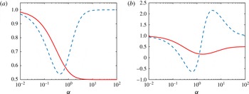
Figure 1 shows examples of the effective TMAC
 $\unicode[STIX]{x1D712}$
and thermal slip coefficient
 $\unicode[STIX]{x1D714}$
in the Epstein model, for
 $\unicode[STIX]{x1D6E9}_{0}=1$
,
 $\unicode[STIX]{x1D6E9}_{1}=0.5$
and
 $\unicode[STIX]{x1D6FC}=\unicode[STIX]{x1D6FD}$
or
 $\unicode[STIX]{x1D6FC}=20\unicode[STIX]{x1D6FD}$
, respectively. When
 $\unicode[STIX]{x1D6FC}$
and
 $\unicode[STIX]{x1D6FD}$
are small, both the TMAC
 $\unicode[STIX]{x1D712}$
and the thermal slip coefficient
 $\unicode[STIX]{x1D714}$
are close to unity. When
 $\unicode[STIX]{x1D6FC}$
and
 $\unicode[STIX]{x1D6FD}$
approach infinity, we have
 $\unicode[STIX]{x1D714}\rightarrow 1$
and
 $\unicode[STIX]{x1D712}\rightarrow \unicode[STIX]{x1D6E9}_{1}$
. Between the two limits,
 $\unicode[STIX]{x1D712}$
and
 $\unicode[STIX]{x1D714}$
can be adjusted over a wide range, by choosing different values of
 $\unicode[STIX]{x1D6FC}$
and
 $\unicode[STIX]{x1D6FD}$
.
The effective TMAC
 $\unicode[STIX]{x1D712}$
(solid lines) and thermal slip coefficient
 $\unicode[STIX]{x1D714}$
(dashed lines) in the Epstein BC. The parameters are
 $\unicode[STIX]{x1D6E9}_{0}=1$
,
 $\unicode[STIX]{x1D6E9}_{1}=0.5$
and (a)
 $\unicode[STIX]{x1D6FC}=\unicode[STIX]{x1D6FD}$
, (b)
 $\unicode[STIX]{x1D6FC}=20\unicode[STIX]{x1D6FD}$
. The viscous slip coefficient is given by
 $(2-\unicode[STIX]{x1D712})/\unicode[STIX]{x1D712}$
.

It will be useful to bear in mind the following points before comparing the numerical and experimental data in § 5. First, like the Maxwell BC, the effective TMAC
 $\unicode[STIX]{x1D712}$
can never be larger than unity in the Epstein BC. Mathematically,
 $\unicode[STIX]{x1D712}>1$
can be achieved by choosing, for example,
 $\unicode[STIX]{x1D6E9}_{0}>1$
. However, this cannot always guarantee the positiveness of the VDF, and therefore will not be considered. This means that, if the experimental TMAC is larger than unity, the Cercignani–Lampis BC must be used. Second, in the Epstein BC the thermal slip coefficient
 $\unicode[STIX]{x1D714}$
can be varied over a wide range, including values above unity, or even negative values. This stands in contrast to the Maxwell and Cercignani–Lampis models, for both of which the thermal slip coefficient is constant, irrespective of the coefficients in the kernel. Therefore, if
 $\unicode[STIX]{x1D714}$
deviates significantly from unity, the Epstein BC should be used. Finally, a (linear) combination of Epstein and Cercignani–Lampis BCs will allow to simultaneously have TMAC above unity, and a wide range for the thermal slip coefficient, see § 5.3.3 below.
4 The linearized Boltzmann equation
In most experiments in gas micro-electro-mechanical systems, the dimensionless pressure and temperature gradients are small (see the first equation in Sharipov & Bertoldo (Reference Sharipov and Bertoldo2009b
)), so that the Boltzmann equation (2.1) can be linearized. For convenience, we introduce dimensionless variables: the spatial coordinate is normalized by the characteristic length
 $\ell$
, temperature is normalized by the wall surface temperature
 $T_{w}$
, velocity is normalized by the most probable molecular speed
 $v_{m}=\sqrt{2kT_{w}/m}$
, molecular number density is normalized by the average number density
 $n_{0}$
and the VDF is normalized by
 $n_{0}/v_{m}^{3}$
.
To calculate the collision kernel for the Lennard–Jones potential (2.5), the intermolecular distance
 $r$
is normalized by
 $d$
, so that the collision kernel can be calculated by the method of Sharipov & Bertoldo (Reference Sharipov and Bertoldo2009a
). The collision kernel is expressed as
 $B(\unicode[STIX]{x1D703},|\boldsymbol{u}|)=|\boldsymbol{u}|\unicode[STIX]{x1D70E}(\unicode[STIX]{x1D703},|\boldsymbol{u}|v_{m})$
, where
 $\unicode[STIX]{x1D70E}(\unicode[STIX]{x1D703},|\boldsymbol{u}|v_{m})$
is exactly the same as the differential cross-section
 $\unicode[STIX]{x1D70E}(\unicode[STIX]{x1D703},E)$
calculated by Sharipov & Bertoldo (Reference Sharipov and Bertoldo2009a
), with the dimensionless relative collision energy
 $E=|\boldsymbol{u}|^{2}kT_{w}/2\unicode[STIX]{x1D716}$
.
In Poiseuille flow, suppose the wall temperature is fixed at
 $T_{w}$
, and a uniform pressure gradient,
 $p=n_{0}kT_{w}(1+\unicode[STIX]{x1D709}_{P}x_{3}/\ell )$
with
 $|\unicode[STIX]{x1D709}_{P}|\ll 1$
, is imposed on the gas in the
 $x_{3}$
direction. Then, the VDF in steady state can be expressed as
 $$\begin{eqnarray}f(x_{1},x_{2},\boldsymbol{v})=f_{eq}(\boldsymbol{v})+\unicode[STIX]{x1D709}_{P}[x_{3}f_{eq}(\boldsymbol{v})+h(x_{1},x_{2},\boldsymbol{v})],\end{eqnarray}$$
where the global equilibrium state is described by
 $$\begin{eqnarray}f_{eq}(\boldsymbol{v})=\frac{\exp (-|\boldsymbol{v}|^{2})}{\unicode[STIX]{x03C0}^{3/2}},\end{eqnarray}$$
and the perturbed VDF
 $h$
satisfies the linearized Boltzmann equation (LBE),
 $$\begin{eqnarray}v_{1}\frac{\unicode[STIX]{x2202}h}{\unicode[STIX]{x2202}x_{1}}+v_{2}\frac{\unicode[STIX]{x2202}h}{\unicode[STIX]{x2202}x_{2}}={\mathcal{L}}(h)-v_{3}f_{eq}(\boldsymbol{v}),\end{eqnarray}$$
with the linearized Boltzmann collision operator
 $$\begin{eqnarray}\displaystyle {\mathcal{L}}(h) & = & \displaystyle n_{0}d^{2}\ell \iint B(\unicode[STIX]{x1D703},|\boldsymbol{u}|)[f_{eq}(\boldsymbol{v}_{\ast }^{\prime })h(\boldsymbol{v}^{\prime })+h(\boldsymbol{v}_{\ast }^{\prime })f_{eq}(\boldsymbol{v}^{\prime })\nonumber\\ \displaystyle & & \displaystyle -\,h(\boldsymbol{v}_{\ast })f_{eq}(\boldsymbol{v})-f_{eq}(\boldsymbol{v}_{\ast })h(\boldsymbol{v})\!]\,\text{d}\unicode[STIX]{x1D734}\,\text{d}\boldsymbol{v}_{\ast }.\end{eqnarray}$$
We use the fast spectral method to solve the collision operator (4.4) and the fast iterative method to solve (4.3) with rapid convergence to the steady state; detailed numerical techniques can be found in Wu et al. (Reference Wu, Liu, Zhang and Reese2015a
, Reference Wu, Zhang, Liu, Zhang and Reese2017). When the VDF
 $h$
is solved, the flow velocity
 $V_{3}$
and the heat flux
 $q_{3}$
, which are normalized by
 $v_{m}$
and
 $n_{0}kT_{w}v_{m}$
, respectively, are calculated as
 $$\begin{eqnarray}\left.\begin{array}{@{}c@{}}\displaystyle V_{3}(x_{1},x_{2})=\int v_{3}h\,\text{d}\boldsymbol{v},\\ \displaystyle q_{3}(x_{1},x_{2})=\int v_{3}\left(|\boldsymbol{v}|^{2}-\frac{5}{2}\right)h\,\text{d}\boldsymbol{v}.\end{array}\right\}\end{eqnarray}$$
The dimensionless MFR and heat flow rate (HFR) in the Poiseuille flow, which are relevant to experimental measurement, are given by
 $$\begin{eqnarray}\left.\begin{array}{@{}c@{}}\displaystyle \text{MFR:}~G_{P}=-\frac{4}{A}\iint V_{3}(x_{1},x_{2})\,\text{d}x_{1}\,\text{d}x_{2},\\ \displaystyle \text{HFR:}~Q_{P}=\frac{4}{A}\iint q_{3}(x_{1},x_{2})\,\text{d}x_{1}\,\text{d}x_{2},\end{array}\right\}\end{eqnarray}$$
where
 $A$
is the cross-sectional area of the flow.
In thermal transpiration flow, a temperature gradient is imposed on the wall in the
 $x_{3}$
direction: the wall temperature is
 $T=T_{w}(1+\unicode[STIX]{x1D709}_{T}x_{3}/\ell )$
with
 $|\unicode[STIX]{x1D709}_{T}|\ll 1$
, but the pressure is fixed at
 $n_{0}kT_{w}$
. In this case, the VDF can be expressed as
 $f=f_{eq}+\unicode[STIX]{x1D709}_{T}[x_{3}f_{eq}(|\boldsymbol{v}|^{2}-5/2)+h]$
, and the perturbed VDF
 $h$
satisfies (4.3), with the source term
 $-v_{3}f_{eq}$
replaced by
 $-v_{3}(|\boldsymbol{v}|^{2}-5/2)f_{eq}$
. In this paper, we do not calculate the thermal transpiration flow, since, according to the Onsager–Casimir relation (Loyalka & Cipolla Reference Loyalka and Cipolla1971), the MFR in thermal transpiration flow,
 $G_{T}$
, is opposite to the HFR in Poiseuille flow,
 $$\begin{eqnarray}G_{T}=-Q_{P}.\end{eqnarray}$$
Note that the dimensionless flow rates are affected by the gas–surface interaction, the intermolecular potential between gas molecules and the rarefaction parameter
 $$\begin{eqnarray}\unicode[STIX]{x1D6FF}=\frac{n_{0}kT_{w}\ell }{\unicode[STIX]{x1D707}v_{m}},\end{eqnarray}$$
where
 $\unicode[STIX]{x1D707}$
is the shear viscosity of the gas. The shear viscosity can be calculated as long as the intermolecular potential is known, details of which can be found in Wu et al. (Reference Wu, Liu, Zhang and Reese2015a
). The dimensionless rarefaction parameter
 $\unicode[STIX]{x1D6FF}$
is related to the inverse of the Knudsen number,
 $\unicode[STIX]{x1D6FF}\sim 1/\text{Kn}$
.
4.1 The linearized boundary conditions
Due to the reciprocity relation (2.6), the BC for the perturbed VDF
 $h$
can be obtained by simply replacing
 $f$
with
 $h$
in (1.1). Since (4.3) possesses the symmetry
 $$\begin{eqnarray}h(x_{1},x_{2},v_{1},v_{2},v_{3})=-h(x_{1},x_{2},v_{1},v_{2},-v_{3}),\end{eqnarray}$$
the Epstein BC can be greatly simplified, as the reflected gas molecules from the surface are only resulting from the specular reflection. Also, in this case, the Klinc & Kuěčer (Reference Klinc and Kuěčer1972) BC is exactly the same with the diffuse BC. Suppose a flat wall is located at the
 $x_{2}$
–
 $x_{3}$
plane and its normal direction is along the
 $x_{1}$
direction. The perturbed VDF for the reflected gas molecules
 $h_{r}$
is related to the perturbed VDF of the impinging molecules
 $h_{i}$
as
 $$\begin{eqnarray}h_{r}(v_{1},v_{2},v_{3})=[1-\unicode[STIX]{x1D6E9}(\boldsymbol{v})]h_{i}(-v_{1},v_{2},v_{3}).\end{eqnarray}$$
For the Cercignani–Lampis BC, the scattering kernel (2.11) is simplified to (Sharipov Reference Sharipov2002, Reference Sharipov2003a ,Reference Sharipov b ):
 $$\begin{eqnarray}R_{CL}(\boldsymbol{v}^{\prime }\rightarrow \boldsymbol{v})=R_{n}(v_{n}^{\prime }\rightarrow v_{n})R_{t}(\boldsymbol{v}_{t}^{\prime }\rightarrow \boldsymbol{v}_{t}),\end{eqnarray}$$
where
 $$\begin{eqnarray}\displaystyle & \displaystyle R_{n}(v_{n}^{\prime }\rightarrow v_{n})=\frac{2v_{n}}{\unicode[STIX]{x1D6FC}_{n}}I_{0}\left(2\frac{\sqrt{1-\unicode[STIX]{x1D6FC}_{n}}v_{n}v_{n}^{\prime }}{\unicode[STIX]{x1D6FC}_{n}}\right)\exp \left\{-\frac{[v_{n}^{2}+(1-\unicode[STIX]{x1D6FC}_{n})v_{n}^{\prime }]^{2}}{\unicode[STIX]{x1D6FC}_{n}}\right\}, & \displaystyle\end{eqnarray}$$
 $$\begin{eqnarray}\displaystyle & \displaystyle R_{t}(\boldsymbol{v}_{t}^{\prime }\rightarrow \boldsymbol{v}_{t})=\frac{1}{\unicode[STIX]{x03C0}\unicode[STIX]{x1D6FC}_{t}(2-\unicode[STIX]{x1D6FC}_{t})}\exp \left[-\frac{|\boldsymbol{v}_{t}-(1-\unicode[STIX]{x1D6FC}_{t})\boldsymbol{v}_{t}^{\prime }|^{2}}{\unicode[STIX]{x1D6FC}_{t}(2-\unicode[STIX]{x1D6FC}_{t})}\right]. & \displaystyle\end{eqnarray}$$
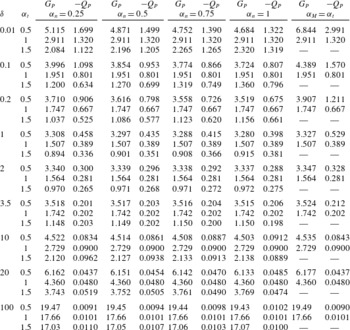
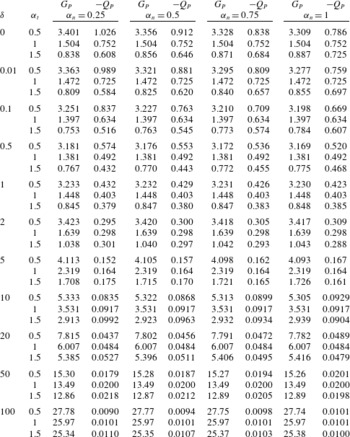
Dimensionless flow rates in the Poiseuille flow of HS molecules between two infinite parallel plates, obtained from the LBE with the Cercignani–Lampis and Maxwell (last two columns) BCs.

4.2 Numerical results using the Cercignani–Lampis boundary condition
In this section, we present solutions of the LBE for the Poiseuille flow between two infinite parallel plates and through a circular cross-section. Although this classical problem has been investigated extensively, accurate numerical results based on the LBE and the Cercignani–Lampis BC are scarce (Garcia & Siewert Reference Garcia and Siewert2009). In our numerical simulations, the accuracy of the flow rates are controlled to within 0.5 % (Wu et al. Reference Wu, Liu, Zhang and Reese2015a ).
We first consider the Poiseuille flow between two infinite parallel plates at a distance
 $\ell$
. Table 1 shows the MFR and HFR for HS molecules, when the Cercignani–Lampis and Maxwell BCs are used. When the parameters
 $\unicode[STIX]{x1D6FC}_{n}$
,
 $\unicode[STIX]{x1D6FC}_{t}$
, and
 $\unicode[STIX]{x1D6FC}_{M}$
in the Cercignani–Lampis and Maxwell BCs are fixed, the HFR always increases when the rarefaction parameter
 $\unicode[STIX]{x1D6FF}$
decreases, while the MFR first decreases and then increases with
 $\unicode[STIX]{x1D6FF}$
, such that the famous Knudsen minimum is observed at
 $\unicode[STIX]{x1D6FF}\approx 1$
.
For the Maxwell BC, when
 $\unicode[STIX]{x1D6FF}$
is fixed, both the MFR and HFR increase significantly when the TMAC
 $\unicode[STIX]{x1D6FC}_{M}$
is reduced. For the Cercignani–Lampis BC, when the values of
 $\unicode[STIX]{x1D6FF}$
and
 $\unicode[STIX]{x1D6FC}_{n}$
are fixed, the MFR also increases rapidly when
 $\unicode[STIX]{x1D6FC}_{t}$
decreases. From (3.3) we know that
 $\unicode[STIX]{x1D6FC}_{t}$
is the effective TMAC of the Cercignani–Lampis BC. By choosing
 $\unicode[STIX]{x1D6FC}_{M}=\unicode[STIX]{x1D6FC}_{t}$
, we see in table 1 that the MFR from the Cercignani–Lampis BC increases slower than that of the Maxwell BC, as
 $\unicode[STIX]{x1D6FC}_{t}$
and
 $\unicode[STIX]{x1D6FC}_{M}$
decrease.
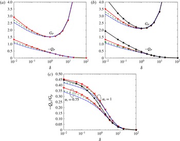
The MFR and HFR in the Poiseuille flow between two parallel plates, when the Cercignani–Lampis and Maxwell BCs are used. Triangles: HS molecules. Dashed lines: helium. Dash-dotted lines: xenon. In the Cercignani–Lampis BC, we use
 $\unicode[STIX]{x1D6FC}_{n}=1$
, (a)
 $\unicode[STIX]{x1D6FC}_{t}=1$
and (b)
 $\unicode[STIX]{x1D6FC}_{t}=0.75$
. In the Maxwell BC,
 $\unicode[STIX]{x1D6FC}_{M}=0.75$
is used (pentagrams). (c) The TPD exponent.

The approximate analytical expression (3.3) predicts no influence of
 $\unicode[STIX]{x1D6FC}_{n}$
on the MFR. From the numerical simulation we see that the influence is indeed very limited. When
 $\unicode[STIX]{x1D6FC}_{t}$
and
 $\unicode[STIX]{x1D6FF}$
are fixed, the MFR decreases slightly when
 $\unicode[STIX]{x1D6FC}_{n}$
increases. For instance, for
 $\unicode[STIX]{x1D6FF}=0.01$
, the MFR is decreased by 10 % when
 $\unicode[STIX]{x1D6FC}_{n}$
is increased from 0.25 to 1; as
 $\unicode[STIX]{x1D6FF}$
increases, this influence becomes weaker and weaker.
The variation of the HFR with respect to
 $\unicode[STIX]{x1D6FC}_{n}$
and
 $\unicode[STIX]{x1D6FC}_{t}$
is more complicated than that of the MFR. First, when
 $\unicode[STIX]{x1D6FC}_{n}$
and
 $\unicode[STIX]{x1D6FF}$
are fixed, the HFR increases slightly with
 $\unicode[STIX]{x1D6FC}_{t}$
at large values of
 $\unicode[STIX]{x1D6FF}$
, while it increases with decreasing
 $\unicode[STIX]{x1D6FC}_{t}$
at small values of
 $\unicode[STIX]{x1D6FF}$
. Second, when
 $\unicode[STIX]{x1D6FC}_{t}=1$
and
 $\unicode[STIX]{x1D6FF}$
is fixed, the HFR does not change with
 $\unicode[STIX]{x1D6FC}_{n}$
: in fact, in this case it can be proven that the Cercignani–Lampis BC is reduced to the diffuse BC (Sharipov Reference Sharipov2002). Third, when
 $\unicode[STIX]{x1D6FC}_{t}(\neq 1)$
and
 $\unicode[STIX]{x1D6FF}$
are fixed, the HFR increases slightly with
 $\unicode[STIX]{x1D6FC}_{n}$
at large values of
 $\unicode[STIX]{x1D6FF}$
, but it increases with decreasing
 $\unicode[STIX]{x1D6FC}_{n}$
at smaller values of
 $\unicode[STIX]{x1D6FF}$
. Similar behaviours have been observed by Sharipov (Reference Sharipov2002) when the linearized Shakhov kinetic model is used instead of the LBE.
The influence of the intermolecular potential between gas molecules is also investigated. For this we choose helium and xenon, since from Sharipov & Bertoldo (Reference Sharipov and Bertoldo2009b
) it is known that the results of other noble gases such as neon, argon and krypton will lie between helium and xenon. Some typical MFR and HFR profiles are shown in figure 2, from which we see that the influence of the intermolecular potential is obvious at small values of
 $\unicode[STIX]{x1D6FF}$
, irrespective of the gas–surface BCs. For small values of
 $\unicode[STIX]{x1D6FF}$
(i.e.
 $\unicode[STIX]{x1D6FF}<1$
), among the HS gas, helium and xenon, the HS gas has the largest MFR and HFR, while xenon has the smallest: in the diffuse BC, the relative differences in the MFR and HFR between HS gas and xenon are approximately 15 % when
 $\unicode[STIX]{x1D6FF}=0.01$
. In the Cercignani–Lampis BC with
 $\unicode[STIX]{x1D6FC}_{n}=1$
and
 $\unicode[STIX]{x1D6FC}_{t}=0.75$
, the relative differences in the MFR and HFR between HS gas and xenon are approximately 12 % and 23 %, respectively, when
 $\unicode[STIX]{x1D6FF}=0.01$
.
Figure 2(c) also shows the TPD exponent, which is an important parameter determining the performance of a Knudsen pump. The TPD exponent is defined as follows: consider a closed system consisting of two reservoirs connected by a long channel. If the temperature ratio
 $T_{1}/T_{2}$
is maintained between the reservoirs, a pressure ratio
 $p_{1}/p_{2}$
is established between them. When the steady state is reached, the two ratios are related to each other as
 $$\begin{eqnarray}\frac{p_{1}}{p_{2}}=\left(\frac{T_{1}}{T_{2}}\right)^{\unicode[STIX]{x1D6FE}},\end{eqnarray}$$
where
 $\unicode[STIX]{x1D6FE}$
is the TPD exponent. If the temperature ratio between the two reservoirs is small, it can be expressed as
 $$\begin{eqnarray}\unicode[STIX]{x1D6FE}=\frac{G_{T}}{G_{P}}=-\frac{Q_{P}}{G_{P}}.\end{eqnarray}$$
It can be found from figure 2(c) that, in the range of
 $\unicode[STIX]{x1D6FF}$
considered, the HS gas has the largest TPD, while xenon has the smallest. This difference increases when
 $\unicode[STIX]{x1D6FF}$
decreases. For instance, in the diffuse BC, the relative difference in TPD exponent between the HS gas and xenon is approximately 8 % when
 $\unicode[STIX]{x1D6FF}=0.01$
. In the Cercignani–Lampis BC, when
 $\unicode[STIX]{x1D6FF}$
is fixed, the TPD exponent decreases with
 $\unicode[STIX]{x1D6FC}_{t}$
. In the Maxwell BC, when
 $\unicode[STIX]{x1D6FC}_{M}$
decreases, the TPD exponent decreases at large values of
 $\unicode[STIX]{x1D6FF}$
, but at small values of
 $\unicode[STIX]{x1D6FF}$
(free molecular flow regime), the TMAC
 $\unicode[STIX]{x1D6FC}_{M}$
does not have any influence on the TPD exponent.
The relative error
 $(G_{Lennard{-}Jones}/G_{HS}-1)\times 100$
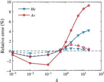
in the MFR between the Lennard–Jones and HS potentials, in the Poiseuille (dashed lines) and thermal transpiration (solid lines) flows through a tube, when the diffuse BC is used.

Dimensionless flow rates in the Poiseuille flow of HS molecules through a circular tube, using the Cercignani–Lampis BC.

Next we consider the Poiseuille flow through a long tube, where the characteristic length
 $\ell$
is chosen as the radius of the circular cross-section. The flow rates are shown in table 2. Unlike to Poiseuille flow between two parallel plates, where the MFR and HFR increase logarithmically as
 $-\ln \unicode[STIX]{x1D6FF}$
when
 $\unicode[STIX]{x1D6FF}\rightarrow 0$
(Takata & Funagane Reference Takata and Funagane2011), both approach constant values when
 $\unicode[STIX]{x1D6FF}\rightarrow 0$
. The influence of the BC on the dimensionless flow rates is similar to that between two parallel plates.
Figure 3 shows the influence of the intermolecular potential on the MFR in the thermal transpiration flow. For
 $\unicode[STIX]{x1D6FF}>0.5$
, the HS model underpredicts the MFR of the Lennard–Jones potentials, for example, when
 $\unicode[STIX]{x1D6FF}=10$
, by approximately 8 % and 4 % for argon and helium, respectively. When
 $\unicode[STIX]{x1D6FF}<0.5$
, however, the HS model overpredicts the MFR. When
 $\unicode[STIX]{x1D6FF}\rightarrow 0$
, the intermolecular potential has no influence on the dimensionless mass flow rate. On the other hand, the influence of the intermolecular potential in the MFR of the Poiseuille flow is within 2 % for all the rarefaction parameters considered.
5 Comparisons between the numerical simulations and experiments
In this section, we solve the LBE (4.3) for the Lennard–Jones potential (2.5), by the method developed by Wu et al. (Reference Wu, Liu, Zhang and Reese2015a , Reference Wu, Zhang, Liu, Zhang and Reese2017). The performance of various gas–surface BCs are compared for Poiseuille and thermal transpiration flows between two infinite parallel plates, and for flows through pipes with rectangular or circular cross-sections, where several experimental data are available (Ewart et al. Reference Ewart, Perrier, Graur and Méolans2007; Rojas-Cárdenas et al. Reference Rojas-Cárdenas, Graur, Perrier and Méolans2013; Yamaguchi et al. Reference Yamaguchi, Rojas-Cárdenas, Perrier, Graur and Niimi2014, Reference Yamaguchi, Perrier, Ho, Méolans, Niimi and Graur2016). We emphasise that the MFR in both Poiseuille and thermal transpiration flows are measured for the same gas and solid surface interactions simultaneously, which provide ideal and strict test cases to the kinetic BCs.
5.1 Thermal transpiration through a rectangular cross-section
Consider the thermal transpiration of helium through a long rectangular channel made of polyether ether ketone (Yamaguchi et al.
Reference Yamaguchi, Rojas-Cárdenas, Perrier, Graur and Niimi2014, Reference Yamaguchi, Perrier, Ho, Méolans, Niimi and Graur2016), where the aspect ratio of the rectangular cross-section is 27.27. For such a large aspect ratio, the numerical simulation based on the Shakhov kinetic model revealed that, when
 $\unicode[STIX]{x1D6FF}\geqslant 0.5$
, there is no difference in the dimensionless flow rates for flows through two infinite parallel plates and rectangular cross-sections (Graur & Ho Reference Graur and Ho2014). Thus, we use the numerical data for flows between two parallel plates to reduce the computational cost, since the experimental measurements are limited to this region of the rarefaction parameter.
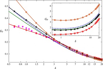
The MFR in the thermal transpiration of helium through a rectangular cross-section of aspect ratio 27.27. Solid dots: experimental data collected from table 1 in Yamaguchi et al. (Reference Yamaguchi, Perrier, Ho, Méolans, Niimi and Graur2016). Pentagrams: the diffuse BC. Squares: the Cercignani–Lampis BC with
 $\unicode[STIX]{x1D6FC}_{n}=0.25$
and
 $\unicode[STIX]{x1D6FC}_{t}=0.5$
. Triangles: the Cercignani–Lampis BC with
 $\unicode[STIX]{x1D6FC}_{n}=0.25$
and
 $\unicode[STIX]{x1D6FC}_{t}=1.75$
. Lines without symbols: the Epstein BC (2.9) with the thermal slip coefficient
 $\unicode[STIX]{x1D714}=0.9$
: dash-dotted line for
 $\unicode[STIX]{x1D6E9}_{0}=0.9$
and
 $\unicode[STIX]{x1D6FC}=0.0192$
, while solid line for
 $\unicode[STIX]{x1D6E9}_{0}=1$
and
 $\unicode[STIX]{x1D6FC}=0.019$
. Other parameters are
 $\unicode[STIX]{x1D6E9}_{1}=0.1$
and
 $\unicode[STIX]{x1D6FD}=\unicode[STIX]{x1D6FC}$
, so that according to (3.4), the effective TMAC
 $\unicode[STIX]{x1D712}$
are 0.85 and 0.95 when
 $\unicode[STIX]{x1D6E9}_{0}=0.9$
and 1, respectively. Inset: the MFR in the Poiseuille flow between two parallel plates.

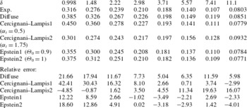
Figure 4 and table 3 compare the experimental data with the numerical results, when the diffuse, Cercignani–Lampis, and Epstein BCs are used. From table 1 we know that, for the Maxwell BC, when
 $\unicode[STIX]{x1D6FF}<3.5$
is fixed, the lowest MFR is reached for
 $\unicode[STIX]{x1D6FC}_{M}=1$
. The comparison with the experiment shows that the diffuse BC overpredicts the MFR by more than 10 %, and choosing other values of the TMAC will increase the prediction error drastically. We then turn to the Cercignani–Lampis BC. From table 1 we know that, for large values of
 $\unicode[STIX]{x1D6FF}$
, better agreement between the simulation and experiment can be achieved when we choose small values of
 $\unicode[STIX]{x1D6FC}_{n}$
and
 $\unicode[STIX]{x1D6FC}_{t}$
, see the squares in figure 4 and data denoted by ‘Cercignani–Lampis1’ in table 3, where
 $\unicode[STIX]{x1D6FC}_{n}=0.25$
and
 $\unicode[STIX]{x1D6FC}_{t}=0.5$
. However, when
 $\unicode[STIX]{x1D6FF}<2$
, the agreement becomes even worse than that of the diffuse BC, for example, for
 $\unicode[STIX]{x1D6FF}=2.22$
and
 $0.998$
, this Cercignani–Lampis BC overpredicts the MFR by approximately 16 % and 42 %, respectively. One can significantly reduce this difference by choosing large values of
 $\unicode[STIX]{x1D6FC}_{t}$
(see triangles in figure 4 and data corresponding to ‘Cercignani–Lampis2’ in table 3, where
 $\unicode[STIX]{x1D6FC}_{n}=0.25$
and
 $\unicode[STIX]{x1D6FC}_{t}=1.75$
), but this increases the error when
 $\unicode[STIX]{x1D6FF}$
is large. For example, when
 $\unicode[STIX]{x1D6FF}>5$
, numerical results overpredicts the MFR by approximately 20 %. This large difference in the slip regime is caused by the fact that the thermal slip coefficient of the Cercignani–Lampis BC is larger than one (Sharipov Reference Sharipov2003a
), which is much larger than the experimental measured value of approximately
 $0.9$
.
The MFR in the thermal transpiration of helium between two infinite parallel plates, using the diffuse, Cercignani–Lampis, and Epstein BCs. The experimental data are collected from table 1 in Yamaguchi et al. (Reference Yamaguchi, Perrier, Ho, Méolans, Niimi and Graur2016). The relative error between the experimental and numerical results is defined as
 $100\times (G_{T}^{numerical}/G_{T}^{exp}-1)$
. The parameters for various BCs are given in figure 4.

The Epstein BC allows more flexibility to choose the velocity slip coefficients and should be able to give better agreement with the experiment. To demonstrate this, we choose the effective thermal slip coefficient
 $\unicode[STIX]{x1D714}$
to be the experimental measured value (Yamaguchi et al.
Reference Yamaguchi, Perrier, Ho, Méolans, Niimi and Graur2016). To achieve this, we choose
 $\unicode[STIX]{x1D6FC}=\unicode[STIX]{x1D6FD}$
in (2.10) for simplicity. We first fix the values of
 $\unicode[STIX]{x1D6E9}_{0}$
and
 $\unicode[STIX]{x1D6E9}_{1}$
, and obtain
 $\unicode[STIX]{x1D6FC}$
and
 $\unicode[STIX]{x1D6FD}$
from (3.5) by setting
 $\unicode[STIX]{x1D714}=0.9$
. We then vary the values of
 $\unicode[STIX]{x1D6E9}_{0}$
and
 $\unicode[STIX]{x1D6E9}_{1}$
, to see the possible influence of different parameters. Our numerical results show that
 $\unicode[STIX]{x1D6E9}_{1}$
has very small influence on the MFR, so in figure 4 and table 3 only the results for
 $\unicode[STIX]{x1D6E9}_{1}=0.1$
are shown. It is clear that for
 $\unicode[STIX]{x1D714}=0.9$
, the simulation results agree well with the experimental data when
 $\unicode[STIX]{x1D6FF}\gtrsim 2$
, for a wide range of
 $\unicode[STIX]{x1D6E9}_{0}$
, see
 $\unicode[STIX]{x1D6E9}_{0}=0.9$
and 1 in figure 4 and table 3. For
 $\unicode[STIX]{x1D6FF}\lesssim 2$
, the value of
 $\unicode[STIX]{x1D6E9}_{0}$
begins to have a strong influence on the MFR: the larger the value of
 $\unicode[STIX]{x1D6E9}_{0}$
, the smaller the MFR in thermal transpiration flow. Taking into account that the experimental data have large errors when
 $\unicode[STIX]{x1D6FF}<1$
(the accuracy of the measurement decreases when the pressure decreases because the physical variation of the pressure is no longer very great with respect to the resolution of the pressure sensor), it seems that the case of
 $\unicode[STIX]{x1D6E9}_{0}=1$
provides good agreement with the experimental measured MFR.
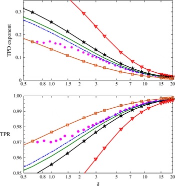
The TPD exponent and TPR in the thermal transpiration of helium through a rectangular cross-section of aspect ratio 27.27. Solid dots: experimental data collected from figure 8 in Yamaguchi et al. (Reference Yamaguchi, Rojas-Cárdenas, Perrier, Graur and Niimi2014). Pentagrams, squares, triangles and lines without symbols: see the parameters in figure 4.

So far, based solely on the comparison in figure 4 and table 3, it is too early to say that the Epstein BC is better than the Cercignani–Lampis BC. In the inset of figure 4 we find that the MFR in Poiseuille flow varies a lot among different BCs. Therefore, the TPD exponent and thermal molecular pressure ratio (TPR) should vary significantly between the two BCs. Fortunately, these two parameters have been measured experimentally using the same gas and solid surface (Yamaguchi et al. Reference Yamaguchi, Rojas-Cárdenas, Perrier, Graur and Niimi2014), which provides an ideal case to assess the accuracy of the Epstein and Cercignani–Lampis BCs.
In the two experiments (Yamaguchi et al.
Reference Yamaguchi, Rojas-Cárdenas, Perrier, Graur and Niimi2014, Reference Yamaguchi, Perrier, Ho, Méolans, Niimi and Graur2016), the temperature difference is small compared to the average gas temperature. Therefore, the TPD exponent can be accurately approximated by (4.15), while the TPR is calculated as follows: in steady state, according to (3.2) in Yamaguchi et al. (Reference Yamaguchi, Perrier, Ho, Méolans, Niimi and Graur2016), the gas pressure
 $p$
along the flow direction satisfies
 $$\begin{eqnarray}\frac{\text{d}p}{\text{d}x_{3}}=-\frac{Q_{P}(\unicode[STIX]{x1D6FF})}{G_{P}(\unicode[STIX]{x1D6FF})}\frac{p}{T}\frac{\text{d}T}{\text{d}x_{3}},\end{eqnarray}$$
where
 $p$
and
 $T$
have been normalized by the initial pressure and the average pressure of the hot and cold reservoirs, respectively. Assuming a linear temperature variation along the rectangular channel, the pressure distribution can be obtained easily; we find that the result does not change even when using the exponential shape of the temperature distribution (Rojas-Cárdenas et al.
Reference Rojas-Cárdenas, Graur, Perrier and Méolans2013), due to the small temperature difference between two reservoirs in the experiments. The TPR is then calculated as the ratio of the pressures of the cold and hot reservoirs.
Figure 5 compares the TPD exponent and TPR between the experimental and numerical results using different gas–surface BCs. It becomes clear that the Epstein BC with
 $\unicode[STIX]{x1D6E9}_{0}=0.9$
(other parameters shown in figure 4) gives the best agreement, while the Cercignani–Lampis BC either overestimates (
 $\unicode[STIX]{x1D6FC}_{t}=1.75$
) or underestimates (
 $\unicode[STIX]{x1D6FC}_{t}=0.5$
) the TPD exponent significantly. For the TPR, the trend is opposite to that of the TPD exponent. We believe the discrepancies between the very Epstein BC and the experimental data when
 $\unicode[STIX]{x1D6FF}<2$
are due to the experimental errors, which become larger and larger as the gas pressure reduces.
5.2 Poiseuille flow through a rectangular cross-section
Consider Poiseuille flow of helium through a silicon microchannel, with a rectangular cross-section of aspect ratio 52.45, subject to a pressure ratio of 5 between the inlet and outlet of the long channel. With such a large pressure ratio, the experimental measurement of the MFR can be made very accurate even in the free molecular flow regimes. This provides a more strict test of the gas–surface BC, as the profile of the perturbed VDF varies significantly at small values of
 $\unicode[STIX]{x1D6FF}$
. For instance, both the theoretical and numerical analysis (Takata & Funagane Reference Takata and Funagane2011; Wu et al.
Reference Wu, Reese and Zhang2014) show that the width of the VDF in the normal direction to the wall surface is proportional to the rarefaction parameter
 $\unicode[STIX]{x1D6FF}$
, when
 $\unicode[STIX]{x1D6FF}\rightarrow 0$
. Thus, the effective TMAC in § 3 obtained using the VDF from the Chapman–Enskog expansion becomes inaccurate.
Since the pressure ratio is not small, the dimensionless MFR
 $G_{P}(\unicode[STIX]{x1D6FF})$
, obtained from the LBE for the Lennard–Jones potential, is transformed to the measured MFR
 $G(\unicode[STIX]{x1D6FF}_{m})$
by (Sharipov & Seleznev Reference Sharipov and Seleznev1994)
 $$\begin{eqnarray}G(\unicode[STIX]{x1D6FF}_{m})=\frac{3}{4\unicode[STIX]{x1D6FF}_{m}}\int _{\unicode[STIX]{x1D6FF}_{m}/3}^{5\unicode[STIX]{x1D6FF}_{m}/3}G_{P}(\unicode[STIX]{x1D6FF})\,\text{d}\unicode[STIX]{x1D6FF},\end{eqnarray}$$
where
 $\unicode[STIX]{x1D6FF}_{m}$
is the gas rarefaction parameter at the average value of the inlet and outlet pressures, with the characteristic flow length
 $\ell$
being the shorter side of the rectangular cross-section.
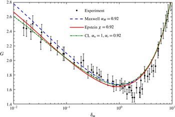
The comparison of the MFR in the Poiseuille flow through a rectangular cross-section of aspect ratio 52.45 with the experimental data (Ewart et al. Reference Ewart, Perrier, Graur and Méolans2007), where the LBE with the Lennard–Jones potential of helium is solved, with the Maxwell, Cercignani–Lampis and Epstein BCs.

At such a large aspect ratio, when
 $\unicode[STIX]{x1D6FF}>1$
, the numerical results for the Poiseuille flow between two parallel plates can be safely used (Graur & Ho Reference Graur and Ho2014). However, when
 $\unicode[STIX]{x1D6FF}<1$
, the numerical simulation is performed in the two-dimensional cross-section: the symmetry is considered and only one quarter of the rectangular cross-section is simulated, which is approximated by
 $31\times 101$
non-uniform cells, with most of the cells adjacent to the surface (Wu et al.
Reference Wu, Reese and Zhang2014).
Figure 6 compares the MFR between the experimental and the numerical results, when the Maxwell, Cercignani–Lampis and Epstein BCs are used. Since in the slip flow regime the measured TMAC is approximately 0.92, we choose
 $\unicode[STIX]{x1D6FC}_{M}=0.92$
in the Maxwell BC,
 $\unicode[STIX]{x1D6FC}_{t}=0.92$
in the Cercignani–Lampis BC with
 $\unicode[STIX]{x1D6FC}_{n}=1$
and
 $\unicode[STIX]{x1D712}=0.92$
in the Epstein BC, together with
 $\unicode[STIX]{x1D6E9}_{0}=1$
,
 $\unicode[STIX]{x1D6E9}_{1}=0.1$
and
 $\unicode[STIX]{x1D6FC}=\unicode[STIX]{x1D6FD}=0.0293$
. At
 $\unicode[STIX]{x1D6FF}_{m}>2$
, the three BCs yield almost identical results. However, as
 $\unicode[STIX]{x1D6FF}_{m}$
decreases, the Cercignani–Lampis and Epstein BCs generate smaller MFRs than the Maxwell BC. For the Epstein BC, this behaviour is easy to understand: as
 $\unicode[STIX]{x1D6FF}$
decreases, the VDF in the normal direction to the wall shrinks (Takata & Funagane Reference Takata and Funagane2011; Wu et al.
Reference Wu, Reese and Zhang2014), so that according to (2.10), fewer gas molecules are specularly reflected than that of the Maxwell BC and the MFR is therefore smaller.
In general, it is seen that the Cercignani–Lampis and Epstein BCs perform better than the Maxwell BC in this special case. But since the MFR in the thermal transpiration flow is not available, it is hard to say which one is best. If only MFR in the Poiseuille flow is concerned, we prefer to use the Epstein BC, since in the discrete velocity method the computational cost for the gas–surface interaction is of the order of
 $N_{v}^{3}$
, while that of the Cercignani–Lampis BC is
 $N_{v}^{6}$
, where
 $N_{v}$
is the number of discretized points in each velocity direction.
5.3 Thermal transpiration through a long tube
Rojas-Cárdenas et al. measured the thermal transpiration flow through a glass tube of circular cross-section (Rojas-Cárdenas et al.
Reference Rojas-Cárdenas, Graur, Perrier and Méolans2013), where, like the thermal transpiration along the channel of rectangular cross-section (Yamaguchi et al.
Reference Yamaguchi, Rojas-Cárdenas, Perrier, Graur and Niimi2014, Reference Yamaguchi, Perrier, Ho, Méolans, Niimi and Graur2016), data of the MFR, TPD exponent and TPR are available. This means that both the viscous and thermal slip coefficients
 $\unicode[STIX]{x1D712}$
and
 $\unicode[STIX]{x1D714}$
in the various BCs need to be adjusted simultaneously, and again, provides a tough assessment of the various BCs.
Before the comparison, it is noted that, according the definitions in Rojas-Cárdenas et al. (Reference Rojas-Cárdenas, Graur, Perrier and Méolans2013) and Yamaguchi et al. (Reference Yamaguchi, Perrier, Ho, Méolans, Niimi and Graur2016), the experimental measured MFR
 $G(\unicode[STIX]{x1D6FF}_{m})$
is related to the simulated MFR
 $G_{T}=-Q_{P}$
as
 $$\begin{eqnarray}G(\unicode[STIX]{x1D6FF}_{m})=2G_{T}(\unicode[STIX]{x1D6FF}_{m})\left(\sqrt{\frac{T_{m}}{T_{C}}}-\sqrt{\frac{T_{m}}{T_{H}}}\right),\end{eqnarray}$$
where
 $\unicode[STIX]{x1D6FF}_{m}$
is the gas rarefaction parameter at the initial gas pressure and mean temperature of the two reservoirs, with the characteristic flow length
 $\ell$
being the radius of the tube.
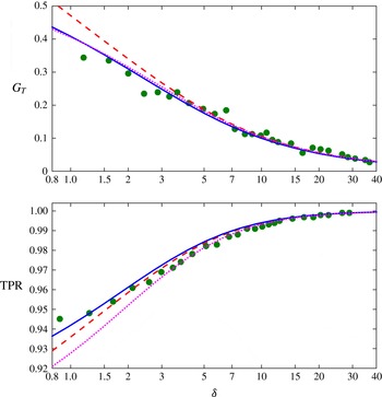
The experiments are conducted for both argon and helium. In the following we consider them separately since different gases have different interactions with the same glass tube. Also, it is noted that when the temperature difference is small, the TPD exponent and the TPR are closely related: if the BC can accurately describe the TPR, it can definitely describe the TPD exponent with good accuracy, see the example in figure 5. For this reason, in the following only the MFR and TPR are considered. Finally, the experimental error is large when
 $\unicode[STIX]{x1D6FF}$
is small, i.e. when the gas pressure is low such that the pressure sensor is no longer very sensitive to the pressure variations and the accuracy of the MFR measurement is reduced. Therefore, in the following, we only analyse the region where
 $\unicode[STIX]{x1D6FF}>2$
.
The MFR and TPR in the thermal transpiration of argon through a circular glass tube. Solid dots: the experimental MFR is adopted from figure 8 in Rojas-Cárdenas et al. (Reference Rojas-Cárdenas, Graur, Perrier and Méolans2013) and has been normalized by (5.3), while the TPR is adopted from figure 9 in Rojas-Cárdenas et al. (Reference Rojas-Cárdenas, Graur, Perrier and Méolans2013) when the temperature difference is 71 K. Solid lines: diffuse BC. Dashed lines: the Epstein BC with
 $\unicode[STIX]{x1D6E9}_{0}=\unicode[STIX]{x1D6E9}_{1}=1$
and
 $\unicode[STIX]{x1D6FC}=20\unicode[STIX]{x1D6FD}=50.6$
, so that the thermal slip coefficient is
 $\unicode[STIX]{x1D714}=1.1$
and the effective TMAC is
 $\unicode[STIX]{x1D712}=0.98$
. Dotted lines: the Cercignani–Lampis BC with
 $\unicode[STIX]{x1D6FC}_{t}=1.2$
and
 $\unicode[STIX]{x1D6FC}_{n}=0.25$
.

5.3.1 Experiment on argon
We solve the LBE with the realistic Lennard–Jones potential for argon. The results of
 $G_{T}$
and TPR for the diffuse BC are shown as solid lines in figure 7. It can be seen that
 $G_{T}$
agrees well with the experimental data, but the TPR is slightly higher than the experimental data at large values of
 $\unicode[STIX]{x1D6FF}$
. This means that, according to (5.1),
 $G_{P}$
should be decreased and/or
 $G_{T}$
should be increased when compared to the diffuse BC. This cannot be realized in the Maxwell BC (since according to table 1, the diffuse BC with
 $\unicode[STIX]{x1D6FC}_{M}=1$
has the minimum MFR in the Poiseuille flow and maximum MFR in the thermal transpiration flow, compared to other Maxwell BC with
 $\unicode[STIX]{x1D6FC}_{M}<1$
), but can be easily done in the Cercignani–Lampis BC by choosing the effective TMAC
 $\unicode[STIX]{x1D6FC}_{t}>1$
. The results for
 $\unicode[STIX]{x1D6FC}_{t}=1.2$
are shown as dotted lines, and good agreement in both
 $G_{T}$
and TPR is observed for
 $\unicode[STIX]{x1D6FF}>2$
. Alternatively, one can use the Epstein BC with the effective thermal slip coefficient
 $\unicode[STIX]{x1D714}>1$
; the results for
 $\unicode[STIX]{x1D714}=1.1$
are shown as dashed lines, which are slightly better than the diffuse BC.
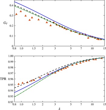
The MFR and TPR in the thermal transpiration of helium through a circular glass tube. Solid triangles: the experimental MFR is adopted from figure 8 in Rojas-Cárdenas et al. (Reference Rojas-Cárdenas, Graur, Perrier and Méolans2013) and has been normalized by (5.3), while the TPR is adopted from figure 9 in Rojas-Cárdenas et al. (Reference Rojas-Cárdenas, Graur, Perrier and Méolans2013) when the temperature difference is 71 K. Solid lines: diffuse BC. Dashed lines: the Epstein BC with
 $\unicode[STIX]{x1D6E9}_{0}=1$
,
 $\unicode[STIX]{x1D6E9}_{1}=0.1$
, and
 $\unicode[STIX]{x1D6FC}=\unicode[STIX]{x1D6FD}=0.019$
, so that the effect thermal slip coefficient
 $\unicode[STIX]{x1D714}=0.9$
and effective TMAC is
 $\unicode[STIX]{x1D712}=0.95$
. Dash-dotted lines: the combined BC (5.4), where
 $\unicode[STIX]{x1D6FC}_{n}=1$
and
 $\unicode[STIX]{x1D6FC}_{t}=1.5$
in the Cercignani–Lampis BC, while
 $\unicode[STIX]{x1D6E9}_{0}=1$
,
 $\unicode[STIX]{x1D6E9}_{1}=0.1$
and
 $\unicode[STIX]{x1D6FC}=\unicode[STIX]{x1D6FD}=0.06$
, so that the thermal slip coefficient is
 $\unicode[STIX]{x1D714}=0.7$
and the effective TMAC is
 $\unicode[STIX]{x1D712}=0.85$
in the Epstein BC.

5.3.2 Experiment on helium
We first solve the LBE with the realistic Lennard–Jones potential for helium, using the diffuse BC. Although the TPR predicted by the numerical solutions agrees well with the experimental data, the MFR
 $G_{T}$
is higher than the experimental measurements, see the solid lines in figure 8. Like the thermal transpiration through the rectangular channel studied in § 5.1, the Cercignani–Lampis BC has difficulty to predict both the MFR and TPR correctly. Therefore, we solve the LBE with the Epstein BC to obtain a good agreement in
 $G_{T}$
first. This is easily achieved when we choose
 $\unicode[STIX]{x1D714}=0.9$
, however, the TPR from the numerical simulation is higher than the experimental ones when
 $\unicode[STIX]{x1D6FF}>2$
, see the dashed lines in figure 8. This means that, according to (5.1), we have to make the effective TMAC in the Epstein BC larger than unity, which is impossible to guarantee the positiveness of the VDF, see the discussion in the end of § 3. Thus, a new kinetic BC is required to describe this experimental data.
5.3.3 A new combined boundary condition
We note that both Epstein and Cercignani–Lampis models are well rooted in arguments based on the physics of the gas–surface interactions, so that their parameters are not merely curve-fitting parameters. Nevertheless, as models, they only approximate the actual behaviour of the molecular collisions. Hence, each model has individual shortcomings which limit its range of application: the Epstein model cannot describe flows with serious ‘backwards’ scattering, for which the viscous slip coefficient
 $(2-\unicode[STIX]{x1D712})/\unicode[STIX]{x1D712}$
is below unity (i.e. the TMAC is above unity), and does not give plume-like structure for reflection of molecular beams; the Cercignani–Lampis model predicts a fixed value
 $(\unicode[STIX]{x1D714}_{CL}=1)$
for the thermal slip coefficient.
For gas–surface interactions where the experimental results indicate viscous slip coefficient and thermal slip coefficient below unity, neither model can be used to model the ensuing flow problems. Since the Epstein BC can adjust the thermal slip coefficient easily (see figure 1), and the Cercignani–Lampis BC can have an effective TMAC (3.3) above unity, we propose to combine them together linearly, that is, to use the following new gas kinetic BC:
 $$\begin{eqnarray}R_{Mix}(\boldsymbol{v}^{\prime }\rightarrow \boldsymbol{v})=\unicode[STIX]{x1D71B}R_{CL}(\boldsymbol{v}^{\prime }\rightarrow \boldsymbol{v})+(1-\unicode[STIX]{x1D71B})R_{E}(\boldsymbol{v}^{\prime }\rightarrow \boldsymbol{v}),\end{eqnarray}$$
to describe the gas–surface interaction, where
 $\unicode[STIX]{x1D71B}$
is a constant with a value between zero and one. Since the only reason to include the Cercignani–Lampis BC into the combined BC is to make the effective TMAC larger than unity, the normal accommodation coefficient
 $\unicode[STIX]{x1D6FC}_{n}$
, which has little effect to the effective TMAC, can be chosen as unity. This will reduce the computational complexity of the BC from
 $N_{v}^{6}$
to
 $N_{v}^{5}$
, where
 $N_{v}$
is the number of discrete velocities in each velocity direction. It should also be noted that the combined model should only be used when significant backwards scattering
 $(\unicode[STIX]{x1D712}>1)$
occurs, which is the case for only a few gas–surface interactions, e.g. the scattering of light molecules by a rough surface such as for the helium flow through a glass tube (Rojas-Cárdenas et al.
Reference Rojas-Cárdenas, Graur, Perrier and Méolans2013), because the computational cost to compute the Epstein model is only
 $O(N_{v}^{3})$
.
Considering that both Epstein and Cercignani–Lampis models have a solid background in physics, and give reliable results within their realm of application, a linear combination of both appears to be the most reasonable approach to maintain the benefits of both, and extend their range of validity. Unfortunately, this increases the number of parameters to be fitted. The new boundary condition has six free parameters:
 $\unicode[STIX]{x1D6FC}$
,
 $\unicode[STIX]{x1D6FD}$
,
 $\unicode[STIX]{x1D6E9}_{0}$
,
 $\unicode[STIX]{x1D6E9}_{1}$
in (2.10),
 $\unicode[STIX]{x1D6FC}_{t}$
in (2.11) with
 $\unicode[STIX]{x1D6FC}_{n}=1$
, and
 $\unicode[STIX]{x1D71B}$
in (5.4). These parameters allows more freedom to fit the experimental data. Following the method in Struchtrup (Reference Struchtrup2013), approximate analytical solutions for the effective TMAC and thermal slip coefficient are derived to guide the comparison, as
 $$\begin{eqnarray}\left.\begin{array}{@{}c@{}}\displaystyle \frac{1}{\unicode[STIX]{x1D712}_{Mix}}=\frac{\unicode[STIX]{x1D71B}}{\unicode[STIX]{x1D712}_{CL}}+\frac{1-\unicode[STIX]{x1D71B}}{\unicode[STIX]{x1D712}_{E}},\\ \displaystyle \unicode[STIX]{x1D714}_{Mix}=\unicode[STIX]{x1D71B}\unicode[STIX]{x1D714}_{CL}+(1-\unicode[STIX]{x1D71B})\unicode[STIX]{x1D714}_{E}.\end{array}\right\}\end{eqnarray}$$
To compare with the experimental data of Rojas-Cárdenas et al. (Reference Rojas-Cárdenas, Graur, Perrier and Méolans2013) on helium, we consider an equal mixture of the Epstein and Cercignani–Lampis BCs, i.e.
 $\unicode[STIX]{x1D71B}=0.5$
in (5.4). We choose
 $\unicode[STIX]{x1D6FC}_{t}=1.5$
in the Cercignani–Lampis BC and
 $\unicode[STIX]{x1D712}=0.85$
and
 $\unicode[STIX]{x1D714}=0.7$
in the Epstein BC, so that according to (5.5), the effective TMAC is
 $\unicode[STIX]{x1D712}_{Mix}\approx 1.1$
and the thermal slip coefficient is
 $\unicode[STIX]{x1D714}_{Mix}\approx 0.9$
. Good agreement between the numerical simulation and experiment is now achieved, see the dash-dotted lines in figure 8.
It should be noted that the parameters used here are chosen from a range of possible choices. This means that our new BC (5.4) still has the freedom to fit other experiments, such as those involving the thermal accommodation coefficient. Unfortunately, there is no experiment measuring the Poiseuille, thermal transpiration and Fourier flows for the same gas and solid surface interaction. Therefore, we leave the further validation of the new BC to future experiments.
6 Conclusions
In summary, various gas kinetic boundary conditions – Maxwell, Cercignani–Lampis, and Epstein – have been assessed by comparing the numerical solution of the linearized Boltzmann equation with recent experimental data on Poiseuille and thermal transpiration flows. To our knowledge, this assessment is the first of its kind, in the sense that (i) mass flow rates in both Poiseuille and thermal transpiration flows are measured for the same gas and solid surface interaction, which poses an ideal and strict test of the boundary conditions and (ii) the linearized Boltzmann equation for the Lennard–Jones potential has been solved accurately, so that the comparison is only affected by the details of the boundary conditions and the accuracy of the experiments. Within the confidence interval of the recent accurate experiments, we found that, although being widely used, the Maxwell and Cercignani–Lampis boundary conditions cannot accurately describe Poiseuille and thermal transpiration flows simultaneously, while the overlooked Epstein model can provide accurate predictions of the mass flow rate as long as the effective TMAC is less than unity.
When the effective TMAC is larger than unity (this corresponds to the backwards scattering to some extent), the Cercignani–Lampis model must be used, since neither the Maxwell model nor the Epstein model can give such a value for the coefficient while guaranteeing the positiveness of the velocity distribution function. For this case a linear combination of the Epstein and Cercignani–Lampis models (5.4) is proposed to describe gas–surface interaction for the Boltzmann equation. Although it contains six free parameters, our approximate analytical expressions for the viscous and thermal slip coefficients provide a useful guidance to select these parameters. It has been found that only the combined boundary condition can reproduce the experimental data of Rojas-Cárdenas et al. (Reference Rojas-Cárdenas, Graur, Perrier and Méolans2013) on the helium flow through a glass tube.
To conclude, if there is no backwards scattering, the Epstein model should be used. Otherwise, our newly proposed boundary condition should be used. Typically, backwards scattering is not a dominant process, and the measured value of the TMAC is below unity. If this is the case, the four-parameter Epstein model promises the best overall description of rarefied flows, since it allows us to fit the TMAC, the thermal slip coefficient and the thermal accommodation coefficient with a less computational cost compared to the Cercignani–Lampis model when solved by the discrete velocity method. Once the free parameters are determined by comparing the numerical solution of the Boltzmann equation with simple experiments, the kinetic boundary condition can be used in gas micro-electro-mechanical systems with complex geometries and flow conditions. This is a practical way to study internal rarefied gas flows until efficient and accurate methods to determine the gas–surface boundary condition become mature. Finally, we point out that the Epstein model and the combined Epstein and Cercignani–Lampis model may also find application at the vapour–liquid interface (Ishiyama, Yano & Fujikawa Reference Ishiyama, Yano and Fujikawa2005; Kon, Kobayashi & Watanabe Reference Kon, Kobayashi and Watanabe2014).
Acknowledgement
L.W. acknowledges the financial support of the Early Career Researcher International Exchange Award from the Glasgow Research Partnership in Engineering, which allows him to visit the University of Victoria and work with H.S. for one month.