


There are two undercurrents to much of the literature on voter turnout: a normative belief that high rates of voter participation are desirable, and an empirical expectation that variation in voter turnout will have electoral consequences. To some extent, these undercurrents flow together. Although one might argue that high turnout is preferable for purely expressive reasons, the typical normative claim asserts that increased levels of voter participation improve the quality of representation by reducing any bias that might result from dissimilarities between voters and nonvoters. Assumed differences between those who vote and those who do not are also at the heart of the commonly hypothesized empirical relationship between aggregate turnout and partisan vote share. As argued originally by the authors of The American Voter (Campbell et al. Reference Campbell, Converse, Miller and Stokes1960, 96–115), if nonvoters and occasional voters hold preferences that differ from those of habitual (or core) voters, then variation in turnout is likely to have meaningful electoral implications. Higher turnout might advantage one party over another, might advantage incumbents or perhaps their challengers, or might lead to greater volatility in the electorate. In turn, each electoral implication from higher turnout is likely to result in significant policy consequences.
Given the potential importance of the link between voter turnout and electoral outcomes, the literature is replete with studies testing the existence and nature of this relationship. Yet, for all the effort, scholarly work has not produced an agreement about whether an empirical association between turnout and electoral outcomes actually exists, nor is there universal agreement regarding the causal mechanism that connects the two phenomena.
Almost all existing studies, for instance, have a partisan component—the most common conjecture being that Democratic candidates typically do better when turnout is high. Some, however, hypothesize that this partisan effect will be conditioned by the partisan composition of the electorate (DeNardo Reference DeNardo1980, Reference DeNardo1986), whereas others find instead that this partisan effect may depend on the presence of class cleavages (Martinez and Gill Reference Martinez and Gill2005). This debate over the causal nature of the relationship between turnout and partisan outcomes is fueled by mixed empirical evidence. Tests of the partisan conjecture vary remarkably in their findings, with Radcliff (Reference Radcliff1994) and Erikson (Reference Erikson1995) anchoring the polar extremes of large partisan (i.e., pro-Democratic) turnout effects and no turnout effects, respectively.
An alternative to the partisan hypotheses is identified by Grofman, Owen, and Collet (Reference Grofman, Owen and Collet1999), who suggest that higher turnout rates could be bad news for incumbents. They note that high turnout “can arise if growing unpopularity of an incumbent leads to an increase in voters who seek to unseat him/her turning out at the polls and/or if potential vulnerability of an incumbent to a successful challenge leads to a campaign by a well-financed challenger whose campaign succeeds in attracting more voters to the polls” (Grofman, Owen, and Collet Reference Grofman, Owen and Collet1999, 359). In this view, high turnout is likely to correspond with decreased vote share for incumbent candidates or the incumbent party. This hypothesized connection between turnout and incumbency is a reasonable alternative (or perhaps complement) to the partisan conjecture, but unfortunately it remains untested. Thus, there exists little scholarly agreement about either the partisan consequences of high turnout or its effect on incumbents in general.
One possible reason for the lingering questions about the effect of turnout on electoral outcomes is that the empirical approaches typically used to assess the relationship allow for claims of correlation but likely do not allow for claims of causation. From classic treatments of the subject (e.g., Burnham Reference Burnham1965; DeNardo Reference DeNardo1980) to more recent studies (e.g., Citrin, Schickler, and Sides Reference Citrin, Schickler and Sides2003; Nagel and McNulty Reference Nagel and McNulty2000), existing scholarship generally investigates the effect of turnout on electoral outcomes using one of two approaches. One set of studies uses survey data on voters and nonvoters to assess the degree to which the latter hold different preferences from the former and thus would have altered the election in question if they had voted (e.g., Citrin, Schickler, and Sides Reference Citrin, Schickler and Sides2003; Highton and Wolfinger Reference Highton and Wolfinger2001; Martinez and Gill Reference Martinez and Gill2005). Another set typically regresses aggregate vote share data on aggregate turnout to assess the effect of turnout on partisan outcomes (e.g., Erikson Reference Erikson1995; Nagel and McNulty Reference Nagel and McNulty1996, Reference Nagel and McNulty2000; Radcliff Reference Radcliff1994).Footnote 1 Establishing a causal relationship between turnout and electoral outcomes—using either approach—is difficult because individual decisions to vote, as well as aggregate turnout data, are likely endogenous to dependent variables involving vote choice. To the extent that the endogeneity problem exists, current analyses suffer from coefficient bias and cannot lead to causal claims. In the end, of course, it is the causal claim that most interests scholars.
In an effort to assess the actual causal effect of variation in voter turnout on electoral outcomes, we employ an instrumental variable approach that uses election day weather—rainfall, to be specific—as an instrument for voter turnout. Election day rainfall is an attractive instrument because it predicts turnout and is exogenous to electoral outcomes. Moreover, we can expect the causal effect of weather-induced variation in turnout to be similar to the general effect of variation in turnout (endogenous or exogenous) resulting from uniformly distributed changes in the costs or benefits of voting. Although our instrument is unlikely to illuminate the causal effect of variation in voter turnout due to targeted mobilization (or suppression) efforts or idiosyncratic candidate characteristics, variation of the sort captured by our instrument is likely to compose a substantial portion of the total variation in voter turnout.
By using county-level data that extend longitudinally from the 1948 to the 2000 U.S. presidential elections, we gain substantial leverage for our weather-based instrumental variable design and, consequently, substantial leverage in uncovering the electoral consequences of turnout variation in recent U.S. elections. Using this approach, we test two previously examined partisan hypotheses: (1) increases in turnout enlarge the vote share of Democratic candidates, and (2) this partisan effect is conditioned by the partisan composition of the electorate. We find substantial support for both hypotheses. In addition, we use the instrumental variable approach to test Grofman, Owen, and Collet's (Reference Grofman, Owen and Collet1999) previously untested hypothesis: (3) increases in turnout decrease the vote share of incumbent candidates/parties. We also propose and test a Volatility Hypothesis: (4) increases in turnout lead to greater electoral volatility. We find substantial support for these latter hypotheses as well, revealing that by narrowly focusing on partisan outcomes, previous scholarship has overlooked two important implications of higher turnout: anti-incumbent voting and general electoral volatility. When we compare the instrumental variable estimates with ordinary least squares (OLS) estimates, it becomes apparent that a failure to address the endogeneity in our model would lead researchers to incorrectly reject all but the Anti-Incumbent Hypothesis.
We conclude by reporting the results of a simulation that varies turnout two percentage points above and below its observed levels. We find that this four-point swing in turnout causes an average change of approximately 20 Electoral College votes per election. Thus, although election-specific factors other than turnout have the greatest influence on who wins an election, variation in turnout appears to exert a significant effect on vote shares at the county, national, and Electoral College levels.
THEORETICAL CONNECTION BETWEEN TURNOUT AND ELECTORAL OUTCOMES
If voters and nonvoters have the same propensities to cast ballots for particular candidates or parties, then turnout levels should not affect who wins elections. This strict condition, however, is unlikely to be met in practice, meaning that variation in turnout will likely result in potentially meaningful changes in electoral outcomes. Exactly how voters and nonvoters differ becomes the crucial question (e.g., Highton and Wolfinger Reference Highton and Wolfinger2001; Wolfinger and Rosenstone Reference Wolfinger and Rosenstone1980), because the nature of these differences will define the political implications of turnout.
We outline the theory behind two well-established hypotheses regarding the effect of turnout on electoral outcomes, one previously proposed but untested hypothesis, and one original hypothesis derived from extant theory. Although our goal here is not to introduce a new, overarching theory of turnout effects from which each hypothesis can be derived, it is theoretically plausible for all four hypotheses to work in consort, instead of in competition. This prospect suggests that the effects of turnout may be more multifaceted than previous scholarship has surmised.
Partisan Effects and the “Two-Effects” Hypothesis
The hypotheses most often discussed in the literature involve the partisan implications of voter turnout. The theoretical rationale positing a partisan bias to turnout begins from an assumption that the same socioeconomic factors that influence whether people vote also correspond with partisan preferences. It is well established in the behavioral literature that U.S. voters tend to be better educated, wealthier, and older than nonvoters, creating a socioeconomic bias in who turns out to vote (e.g., Leighley and Nagler Reference Leighley and Nagler1992). These same social factors have also been fairly stable predictors of support for the Republican Party and its candidates (Gelman et al. Reference Gelman, Park, Shor, Bafumi and Cortina2008). So, it is reasonable to assume that those who are likely to vote are also more likely to sympathize with Republican candidates than those who are not likely to vote. Elections in which only high probability voters turn out at the polls should exhibit the greatest pro-Republican bias. As turnout rates increase—resulting from lower probability voters casting ballots—this partisan bias should decrease.Footnote 2 Thus, the logic underlying the Partisan Effect Hypothesis corresponds with the conventional wisdom that Democratic candidates do better when turnout is high.Footnote 3
Partisan Effect Hypothesis: Increases in turnout will lead to increases in the Democratic candidate's vote share.
In what is arguably the best known work on the effect of turnout on vote share, DeNardo (Reference DeNardo1980, Reference DeNardo1986) concedes that Democrats will benefit from higher turnout on average, but argues that this effect is conditional. DeNardo contends that the electorate is composed of two types of voters: those who regularly vote (“core voters”) and those who occasionally vote (“peripheral voters”).Footnote 4 Although core voters have strong partisan attachments, peripheral voters have much weaker partisan leanings and tend to be more vulnerable to short-term electoral forces. Consequently, peripheral voters are more likely to defect from their weakly held partisan allegiances. As a result, the partisan composition of an electorate will influence the partisan effect of higher turnout.Footnote 5
As an extreme example, consider a county in which every registered voter identifies as a Democrat. In a low turnout election, core voters, who are likely to be dedicated Democrats, are most likely to turn out, and the vote share for a Democratic candidate should be close to 100%. In a high turnout election, where peripheral voters with weaker commitments to the Democratic Party are voting, a meaningful proportion of these added voters are likely to defect and vote for the Republican. Thus, higher turnout in this county will increase the vote share for the Republican candidate. Of course, the underlying mechanism works in exactly the same way if we alternate the Republican and Democratic labels in the given example. The point to be made here is that high turnout does not necessarily benefit the Democratic Party as the Partisan Effect Hypothesis (and conventional wisdom) suggests. As our extreme example illustrates, the partisan composition of an electorate will condition the effect of the level of voter turnout if peripheral voters are more likely to defect than core voters.
Thus, DeNardo contends that turnout has “two effects.” Higher turnout will generally help Democratic candidates, but higher turnout also helps the minority party within an electorate. More precisely, the positive marginal effect of turnout on Democratic vote share should decrease in size as the proportion of Democrats in the electorate increases. In Republican-dominated electorates, Democratic candidates will be particularly helped by higher turnout because both the introduction of more Democratic voters and weak Republican identifiers will push Democratic vote share upward. The more Democratic the electorate, the less helpful higher turnout will be for a Democratic candidate. In fact, in particularly Democratic electorates, higher turnout could increase the Republican candidate's vote share.
Two-Effects Hypothesis: The more Republican an electorate, the more that increases in turnout will increase Democratic vote share. In particularly Democratic electorates, increases in turnout may decrease Democratic vote share.
The Anti-incumbent Effect
Grofman, Owen, and Collet (Reference Grofman, Owen and Collet1999) offer a third hypothesis involving the political implications of turnout. Although careful not to make a causal claim, they argue that higher turnout will be associated with lower vote share for the incumbent party.Footnote 6 In our view, there are two plausible justifications for this expectation. First, the conditions that cause voters to reject the incumbent party may also cause more voters to turn out at the polls. A troubled economy or unpopular war effort, for example, may stimulate both higher turnout and a collective vote against the incumbent candidate or party. In this situation, however, turnout and an anti-incumbent vote are associated, but the former does not cause the latter.
A second potential justification for this hypothesis builds on the assumption that core voters differ from peripheral voters. Here, the operative difference between these groups is not partisan, ideological, or socioeconomic. Instead, the assumption is that core voters are on average more supportive of the governmental status quo than peripheral votes because they played a more active role in establishing the status quo in previous elections.Footnote 7 By definition, occasional voters or perpetual nonvoters had a lesser hand in the formation of the status quo. The more that these voters are involved in an election, the worse the incumbent party's candidate will do. This justification for Grofman, Owen, and Collet's (Reference Grofman, Owen and Collet1999) hypothesis clearly draws a causal arrow from turnout to the vote share of the incumbent party's candidate. Because we are interested in causal claims about turnout, we rely on this second rationale:
Anti-Incumbent Hypothesis: Higher turnout will decrease the vote share of the incumbent party's candidate.
The Volatility Effect
Because peripheral voters tend to possess weaker partisan attachments and weaker affinity toward incumbents, it is likely to be more difficult to predict exactly how they will vote if and when they do come to the polls. Consider DeNardo's defection argument. He contends that peripheral voters are more likely to defect from whatever partisan leanings they may possess. If this is the case, one wonders what criteria peripheral voters do rely on when making an electoral choice. It is unlikely that peripheral voters vote based on policy preferences or ideology. In fact, Highton and Wolfinger (Reference Highton and Wolfinger2001) find—relying on American National Election Study (ANES) data—that those who did not vote in the 1992 and 1996 elections were less likely to view themselves ideologically, had weaker policy opinions, and were more likely to view themselves as independents than those who did vote. Thus, not only are peripheral voters more likely to defect from their weakly held partisan leanings, but they are also less likely to vote based on policy preferences or ideology. This suggests that DeNardo's defection argument can be expanded beyond its original specification: peripheral voters not only have weaker levels of partisan attachment, but they also generally have weakly held political attitudes that play a minimal role in determining their vote. Consequently, we suspect that if these typical nonvoters actually do vote, their votes will be less predictable than those cast by ideological partisans with strong policy preferences.Footnote 8
High levels of turnout result from occasional voters and some perpetual nonvoters heading to the polls. This, in turn, means that a larger proportion of the electorate is nonideological, independent, and holds weak policy preferences. If these additional voters are less predictable in terms of their vote choice, then high turnout elections ought to be less predictable in the aggregate than low turnout elections.
Volatility Hypothesis: As turnout increases, vote share will become less predictable.
CURRENT APPROACHES TO ESTIMATING TURNOUT EFFECTS AND THE PROBLEM OF ENDOGENEITY
Scholars have employed two different strategies when analyzing the political implications of voter turnout. The first approach uses aggregate data and regresses partisan vote share on levels of voter turnout. The results of these studies are quite mixed, with some finding strong support for what we label partisan effects (e.g., Radcliff Reference Radcliff1994), some finding no support for partisan effects (e.g., Erikson Reference Erikson1995), and others providing evidence for the Two-Effects Hypothesis (e.g., Nagel and McNulty Reference Nagel and McNulty1996, Reference Nagel and McNulty2000).
The problem with this approach is that it assumes that levels of voter turnout are exogenous to partisan vote share. Yet, it is likely that voter turnout is actually endogenous. Downs's (Reference Downs1957) seminal work on the logic of voter turnout implies as much. First, Downs's calculus of voting suggests that eligible voters decide whether to vote based in part on the extent to which one candidate is preferable (i.e., provides greater expected benefits) to the other. If some segment of voters sees no (or little, if there is a cost to voting) difference in expected utility between the candidates, Downs's model predicts that it is rational for these voters to abstain (1957, 39). Of course, the relative utility of the candidates also determines for whom a voter chooses to vote. In other words, a voter's relative preferences regarding the candidates, and thus the likely direction of the vote, affect his or her decision to vote in the first place.
A second way in which Downs's logic suggests endogeneity is via the perceived closeness of the election. As the perceived probability of a close election increases, the instrumental value of voting also increases and turnout levels should rise (Nicholson and Miller Reference Nicholson and Miller1997). Moreover, in close elections, candidates and parties also have a greater incentive to mobilize voters, another possible source of higher turnout (Cox Reference Cox1988). Consequently, this could cause high turnout to appear to cause close elections when the reverse relationship is more likely.
Although mobilization efforts may intensify during close elections, parties and candidates are likely to engage in some mobilization efforts regardless of the expected closeness of the campaign (Rosenstone and Hansen Reference Rosenstone and Hansen1993). These mobilization efforts alone could also contribute to the endogeneity problem. If, by example, the Republican Party's mobilization efforts target Republicans in heavily Republican areas, while the Democratic Party targets Democrats in heavily Democratic areas, then high turnout might appear to favor the Republican candidate in Republican areas and the Democratic candidate in Democratic areas, even though turnout was boosted in these areas as a function of anticipated vote share.
The second approach scholars have taken when analyzing the political implications of voter turnout is to use individual-level survey data to simulate what would have happened if nonvoters had decided to vote in the election (e.g., Citrin, Schickler, and Sides Reference Citrin, Schickler and Sides2003; Highton and Wolfinger Reference Highton and Wolfinger2001; Martinez and Gill Reference Martinez and Gill2005). The appeal of this approach is that researchers can use data on the preferences of nonvoters to project how they might have voted. The problem, of course, is that these projections are not testable, and it is not necessarily clear how to forecast what nonvoters would do at the polls. Moreover, there is still the issue of endogeneity. For example, it is possible that nonvoters chose not to vote because there was not a candidate for whom they wanted to vote. Assigning preferences to these individuals may be presumptuous.
The main point here is that the decision to turn out cannot be simply assumed to be exogenous to vote choice. At both the individual and aggregate levels, turnout is likely endogenous to vote choice. If endogeneity exists, then the coefficient estimates of existing analyses are biased, and any attempt to infer a causal relationship between turnout and the vote will be invalid. In sum, prior work has not been able to provide a clear, causal connection between level of turnout and electoral outcomes.
AN INSTRUMENTAL VARIABLE APPROACH TO ESTIMATING TURNOUT EFFECTS
Instrumental variables regression analysis (IV) was developed explicitly for situations in which an independent variable is potentially endogenous.Footnote 9 This approach begins with the identification of a variable (or set of variables) that will serve as an instrument for the endogenous variable. The endogenous independent variable is then regressed on the instrument(s), and the results of this regression are used to predict values of the endogenous variable. These predicted values are then included as an independent variable in the main model of interest. Proper identification of the IV model requires that the model of the endogenous “independent” variable must include a subset of instruments that are excluded from the main model (consequently, we refer to such an instrument as an “excluded instrument”). Model identification also requires that there must be at least as many excluded instruments as there are endogenous independent variables in the main model. As long as the excluded instruments are (1) uncorrelated with the error term in the main equation (i.e., are exogenous to the dependent variable in the main model) and (2) correlated with the endogenous independent variable, then IV produces consistent coefficient estimates of the effect of the endogenous independent variable on the dependent variable.
For our model, the primary task is to identify an appropriate instrument for aggregate voter turnout. No such instrument has been recognized in the literature. One might assume that registration laws, such as closing dates, Motor Voter laws, and the like, might serve as suitable instruments for turnout, but none of these variables is clearly exogenous to electoral outcomes.Footnote 10 We believe that we have found a useful instrument for pursuing an IV approach to estimating the effect of turnout on electoral outcomes—election day weather. Recent work by Gomez, Hansford, and Krause (Reference Gomez, Hansford and Krause2007) validates the long-held belief that bad weather on election day is associated with lower levels of voter turnout, and bad weather is clearly exogenous to electoral outcomes. These properties suggest that election day rainfall—our operationalization of weather—should serve as a suitable excluded instrument for turnout. To determine whether this instrument has sufficient explanatory power, the econometric literature indicates that an F-test statistic of at least 10 for an excluded instrument or set of excluded instruments should be obtained for the main equation estimates to be consistent (see Staiger and Stock Reference Staiger and Stock1997). For each of our analyses, we provide the relevant F-test statistic. Each F statistic clearly exceeds the threshold of 10, further validating our choice of election day rainfall as an instrument for voter turnout.Footnote 11
Before proceeding, however, we must confront an important issue at the nexus of theory and method. Although our weather-based instrument leverages exogenous variation in voter turnout to identify the causal effect of turnout on electoral outcomes, we need to consider the extent to which our IV approach will illuminate the electoral implications of endogenous sources of variation in voter participation. After all, one might ask (1) whether “variation in the endogenous regressor related to [our] instrumental variable [has] the same causal effect as variation unrelated to [our] instrument” (Dunning Reference Dunning2008, 291) and (2) whether the effect we capture is politically relevant.
The first question presumes that turnout can be divided into two components, TO 1 and TO 2, where the former includes all variation in turnout (exogenous and endogenous) that has the same effect on vote shares as the variation exogenously determined by election day weather, and the latter includes variation in turnout that has an alternative effect. The question is: how much variation is contained by each component? Without additional instruments to allow us to test empirically whether different components of the variation in voter turnout have similar or different effects on vote shares, we must rely on theory to answer this question (Dunning Reference Dunning2008, 301).
At one extreme, TO 1 could consist only of weather-determined turnout. At the other, TO 1 could contain turnout in its entirety, meaning that our IV estimates represent the effect of any and all variation in turnout on electoral outcomes. Neither extreme is realistic. Theoretically, the causal effect of weather-induced variation in turnout should be similar to the effect of all variation in turnout (endogenous or exogenous) resulting from uniformly distributed changes in the costs or benefits of voting that particularly alter the turnout decisions of peripheral voters, who “sit the fence” between voting and staying home. This would include variation in turnout that results from any general change to the costs and benefits of voting that is not politically targeted (i.e., that does not target potential voters based on their likely vote choice) or determined by the appeal of a specific candidate. Importantly, variation of this type (i.e., nontargeted and non–candidate-generated variation) likely represents a significant portion of the overall variation in voter turnout. For instance, alterations in registration or voter identification requirements represent changes in costs that are meted out equally across all eligible voters, and thus should be considered within TO 1. Research shows that changes in electoral laws are powerful predictors of aggregate voter turnout (see Geys Reference Geys2006; Rosenstone and Wolfinger Reference Rosenstone and Wolfinger1978). Another important source of variation in turnout that should fall into TO 1 is the closeness of the electoral contest (see Geys Reference Geys2006). Because a close race increases the probability that any one vote will be influential, all voters will experience a change in their calculus of participation. These changes may be determinative for peripheral voters for whom a slight change in the benefits (or costs) of voting determines whether they turn out. Thus, a close race increases their turnout just as a sunny election day does. Expansive changes in the information environment are likely to uniformly reduce the cognitive costs (or increase the perceived benefits) of becoming engaged with and informed about the political world (Berinsky Reference Berinsky2005). Changes of this sort will affect the utility calculations of all voters and may be pivotal in activating peripheral voters. Finally, mobilization efforts that are not politically targeted, such as general get-out-the-vote (GOTV) appeals, can increase turnout (e.g., Gerber and Green Reference Gerber and Green2000). The increase in turnout resulting from these efforts is a function of adding marginal voters (see Arceneaux and Nickerson Reference Arceneaux and Nickerson2009), who should behave in much the same way as additional voters spurred on by a pleasant election day. In sum, our IV estimates should capture the causal effect of much of the politically interesting variation in turnout, exogenous and endogenous.
Variation in voter turnout attributable to candidate characteristics or mobilization (or suppression) efforts that target particular types of voters will likely have different electoral effects, however. For example, if the presence of a particularly charismatic candidate on the ballot causes an increase in turnout, this increase may not have the same consequences as variation in turnout generated by non–candidate-driven changes to the benefits or costs of voting. Similarly, if a candidate or party can effectively target and mobilize core supporters, any resulting increase in turnout will probably benefit that candidate or party, producing a potentially asymmetric effect on vote share. Of course, it is possible, if not likely, that the mobilization efforts of one party may be counteracted by similar activities by the opposition, indicating that increases in turnout due to this mechanism may have little or no net effect on electoral outcomes. Both types of influence on turnout should fall into TO 2, meaning that we cannot infer that our IV results apply to this type of variation in turnout.
Which type of determinant of turnout is of greater importance? Put differently, which is larger, TO 1 or TO 2? Again, we have no way to answer this question empirically because the absence of an exogenous instrument for TO 2 makes a direct comparison impossible. We do believe it important, though, that two of the best systematic predictors of changes in aggregate-level turnout—changes to registration requirements and the anticipated closeness of the election—should have electoral effects similar/to those revealed by our IV model. In short, our IV results should apply well beyond the electoral consequences of truly exogenously determined variation in turnout, but may not encompass all possible sources of variation in turnout.
DATA
Our data set consists of observations from the nearly 2,000 non-Southern counties in the continental U.S. for each presidential election from 1948 to 2000.Footnote 12 Our unit of analysis is thus the county election dyad. This low level of aggregation is particularly useful given that the excluded instrument we use for turnout is rain on election day. A larger unit of aggregation, such as the state, would prevent an accurate measure of rainfall, potentially muting the correlation between weather and turnout, and would thus hurt the power of this critical instrument. The inclusion of a substantial number of elections also guarantees a good deal of variation in election day weather.Footnote 13
Studies examining turnout effects usually exclude the South. In our case, we exclude Southern counties for three reasons.Footnote 14 First, both voter turnout and presidential vote share are problematic in Southern states for the first half of our time span. Formal and informal barriers to voting depressed turnout until federal actions largely removed them. At the same time that these barriers were being overcome, the South experienced a major partisan realignment, which may lead to a spurious relationship between turnout and electoral outcomes (see Erikson Reference Erikson1995). This is quite important. Erikson (Reference Erikson1995) argues that previous studies demonstrating a correlation between turnout and the vote are primarily driven by political change in the South. He argues that when analyses are restricted to non-Southern states there is “no evidence whatsoever of a turnout effect on the vote” (Erikson Reference Erikson1995, 387). A second justification for restricting our data is that regional third-party candidates garnered substantial electoral support in the South during a few of our earlier elections, making it difficult to analyze two-party vote share.Footnote 15 Third, F tests reveal that rainfall does not have the same explanatory power when it comes to voter turnout in Southern counties, as it does for non-Southern counties. In fact, for Southern counties, rainfall does not produce F statistics that meet the minimum threshold for properly estimating an IV model.
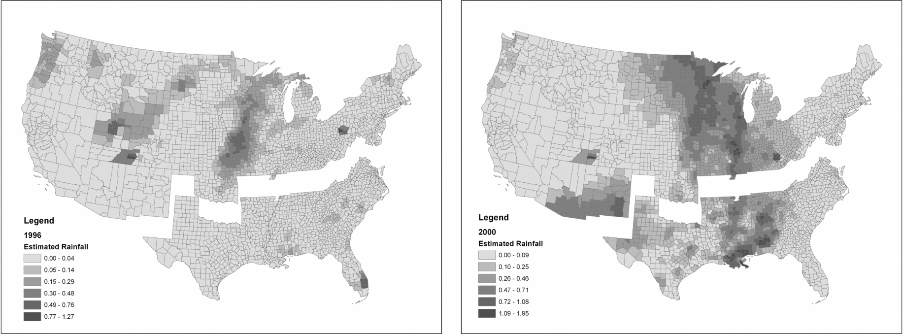
The dependent variable in our initial analyses is the percentage of the two-party vote received by the Democratic presidential candidate.Footnote 16 To measure our excluded instrument, rainfall on election day, we use the National Climatic Data Center's “Summary of the Day” data (made available by EarthInfo, Inc.). The Summary of the Day data report various measures of daily weather for more than 20,000 weather stations located in the U.S. Despite the sizeable number of meteorological observations, not all U.S. counties have weather stations situated within their borders, whereas many counties have multiple weather stations. We therefore used a geographic information system (GIS) method known as Kriging to estimate election day rainfall, in inches, for each county (see Childs Reference Childs2004).Footnote 17 To provide a sense of what these rainfall data “look like,” Figure 1 presents rainfall maps for the 1996 and 2000 elections, the two most recent elections in our analysis.
Estimated Rainfall during the 1996 and 2000 Elections

It is likely that the behavioral effect of election day rain depends on the typical weather conditions experienced in a county on that day. For this reason, we also calculated the normal (average) rainfall for each election date (ranging from November 2 to 9) for each county using data from the entire 1948–2000 time span. We then subtracted the county's normal rainfall from the rainfall estimated to have occurred on each respective election day under analysis. By measuring Rain as a deviation from its normal, we account for typical regional variations in weather.Footnote 18 As we discuss in the previous section, this measure will serve as our excluded instrument for voter turnout.Footnote 19
Two of the hypotheses we seek to test require additional independent variables: partisan composition of the county and party of the incumbent president. Partisan Composition is measured as the moving average of the two-party Democratic vote share (i.e., percentage of the two-party vote cast for the Democratic presidential candidate) in the county in the three most recent elections. For county C in presidential election E, this variable equals the average of C's Democratic vote share in E-1, E-2, and E-3. The Two-Effects Hypothesis indicates that partisan composition conditions the effect of turnout on Democratic vote share. We therefore include the interaction of this variable with turnout and expect a negative estimate for this multiplicative term (indicating that the more Democratic a county, the less that increases in turnout add to Democratic vote share). To include an interaction term involving an endogenous variable, we need to create a second excluded instrument.Footnote 20 We thus include in our IV model the product of our rain variable and the partisan composition measure as a second excluded instrument predicting the product of turnout and partisan composition.Footnote 21 This strategy provides us with consistent estimates of the conditioning influence of partisan composition on the effect of turnout on vote shares.
Our incumbency variable is a dummy variable that equals one if the incumbent president is a Republican. The Anti-Incumbent Hypothesis suggests that the candidate of the same party as the incumbent president will be hurt by higher turnout. To test this hypothesis, we need to interact the Republican Incumbent variable with turnout. We expect the coefficient estimate associated with the interaction term to be positive (indicating that turnout increases Democratic vote share when the incumbent is a Republican). Again, for our IV model, we must create an instrument for this interaction term, so we use the product of rainfall and the dummy variable for Republican incumbent as an additional excluded instrument predicting the product of turnout and Republican incumbent. Note that the dummy variable indicating a Republican incumbent is not included in the model on its own (as a constitutive term) because this effect is already accounted for by our inclusion of election-specific fixed effects, which we discuss as follows. For a presentation of the three first-stage models (predicting turnout, turnout × partisan composition, and turnout × Republican incumbent), as well as an alternative IV approach to incorporating interaction terms including an endogenous variable, see the Appendix.
There are obviously many other factors that may influence a county's Democratic vote share in any given election. Our strategy for controlling these other potential influences is to include fixed effects for both counties and elections. These fixed effects should account for potential heterogeneity in the data and the accompanying correlation of residuals, while providing us with conservative coefficient estimates for our variables of interest.Footnote 22 Given that the Volatility Hypothesis implies heteroskedastic residuals, we estimate robust standard errors. As we discuss later in some detail, we also consider the potential problem posed by spatial autocorrelation.
For the purpose of comparison, we also use OLS to estimate our model with actual turnout instead of instrumented turnout. Our measure of voter turnout in each county is calculated by dividing the number of votes cast at the presidential level by the estimated voting age population.Footnote 23 We provide these parallel model estimations in order to assess the consequences of treating turnout as exogenous.
RESULTS
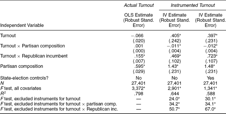
The results of the OLS and IV models explaining the two-party vote share of Democratic presidential candidates are presented in Table 1. The first column in Table 1 presents the OLS estimates for the model when actual, not instrumented, turnout is included as the key independent variable. Based on these estimates, we would conclude that increases in turnout lead to increases in Democratic vote share if there is a Republican incumbent. Thus, the OLS results support the Anti-Incumbent Hypothesis, but not the others. Of course, the OLS evidence in support of the Anti-Incumbent Hypothesis is itself suspect. If we had only estimated the OLS model, a skeptic would rightfully question the causal connection between incumbency and turnout. After all, it is quite possible that high turnout occurs because voters are dissatisfied with the incumbent president's performance. Davidson and MacKinnon's (Reference Davidson and MacKinnon1993) endogeneity test reveals, as suspected, that the OLS estimates using actual turnout suffer from endogeneity.Footnote 24 The OLS estimates are thus not consistent, and the IV estimates we discuss below are preferred.Footnote 25
County-level Democratic Vote Share in Presidential Elections, 1948–2000

Notes: Fixed effects for counties and for election years are included in all models. Southern counties are excluded from the analysis.
*p ≤ .05 (one-tailed test).
The second column of results in Table 1 presents the estimates for our fixed effects IV model.Footnote 26 An initial examination of these IV coefficient estimates and their standard errors reveals three tentative conclusions.Footnote 27 First, when the partisan composition of a county is 0% Democratic—a purely hypothetical condition—and there is a Democratic president in office, the estimated effect of voter turnout is positive and (barely) statistically significant. Thus, in the most Republican county imaginable, increases in turnout lead to increases in Democratic vote share. This conclusion is solely based on the estimate for the constitutive turnout variable, which captures the effect of turnout when the two conditioning variables equal zero. Of course, not much should be made of this particular result, given that counties are never 0% Democratic.
Second, the coefficient estimates from this IV model also indicate that the positive effect of turnout on a Democratic candidate's vote share decreases as a county becomes more Democratic in composition. This conditional relationship is indicated by the negative and statistically significant estimate for the interaction term involving partisan composition. According to DeNardo (Reference DeNardo1980, Reference DeNardo1986), high levels of turnout mean that more peripheral voters are voting. These voters are, by nature, more likely to defect from their loosely held partisan ties, a tendency that benefits the minority party in the county. The IV results support both of DeNardo's “two effects”—increases in turnout simultaneously help both Democrats and the minority party in the electorate in question. To be sure, prior work has provided evidence compatible with DeNardo's hypothesis (Nagel and McNulty Reference Nagel and McNulty1996, Reference Nagel and McNulty2000), but this is the first evidence that variation in turnout exerts this conditional causal effect on vote share. It is important to note that the OLS estimates presented in Column 1 “miss” this effect.
A third inference to be drawn from these IV estimates is that turnout exerts a larger positive effect on Democratic vote share when the incumbent president is a Republican. The positive and statistically significant estimate for the interaction term including the Republican incumbent dummy variable reveals this effect. This finding supports the Anti-Incumbent Hypothesis, which is based on the assumption that marginal voters are less supportive of the incumbent party (i.e., party of the president in office) than dedicated voters. According to this hypothesis, the positive effect of turnout on Democratic vote share should be conditioned by whether the incumbent president is a Republican or a Democrat. Our evidence shows this to be the case. Although this particular result is also obtained with the OLS model, these IV results provide greater confidence in the causal claim that higher turnout lowers vote share for the candidate of the incumbent's party.
To gain a full picture of these IV results and a clear understanding of their implications for the hypotheses tested, we computed the full range of conditional coefficients and the accompanying conditional standard errors in the IV model. Given the presence of the two interaction terms, the effect of voter turnout on a Democratic presidential candidate's vote share is a combination of the coefficient estimates for the constitutive term and the two interaction terms. Specifically, the estimated effect (the conditional coefficient) of voter turnout is [.405 – (.011 × partisan composition) + (.469 × Republican incumbent)]. This can be further simplified by separately considering situations in which the incumbent president is a Republican and those in which the incumbent is a Democrat. With a Republican incumbent, the conditional coefficient for turnout is [(.405 + .469) – (.011 × partisan composition)]. With a Democratic incumbent, the coefficient is [.405 – (.011 × partisan composition)].
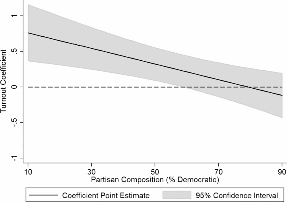
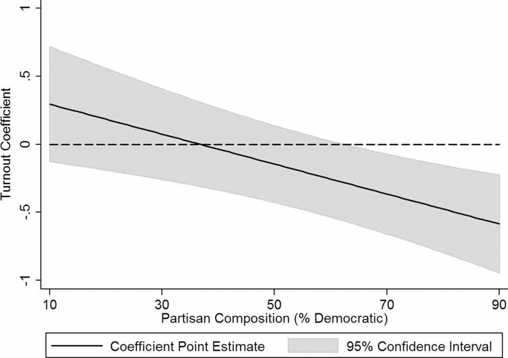
Figures 2 and 3 graphically illustrate the marginal effect (i.e., coefficient) of turnout on Democratic vote share, conditional on the partisan composition of the county. In Figure 2, the coefficients correspond to the presence of a Republican incumbent, whereas the coefficients in Figure 3 are calculated with a Democratic incumbent. For both figures, partisan composition ranges from 10% to 90% Democratic, a range of values closely approximating the actual range found in our data.
Coefficient for Turnout, Conditional on Partisan Composition (Republican Incumbent)

Coefficient for Turnout, Conditional on Partisan Composition (Democratic Incumbent)

When there is a Republican incumbent (a condition that is true in 7 of our 14 elections), turnout has a positive effect on Democratic vote share (i.e., the point estimate for the coefficient is greater than zero) as long as the county in question is less than 80% Democratic. This effect is statistically significant for all values of partisan composition less than 60%.Footnote 28 Put differently, increases in turnout generally help the Democratic candidate when there is a Republican in office. The magnitude of the effect is attenuated, though, by the partisan composition of the county. The more Democratic the county, the less that turnout helps the Democratic candidate. This declining conditional marginal effect (exhibited in Figure 2) is entirely consistent with DeNardo's Two-Effects logic and demonstrates that changes in turnout do simultaneously help both Democrats and the minority party in the electorate.
Interestingly, when there is a Democratic incumbent, as shown in Figure 3, turnout never has a positive and statistically significant effect on Democratic vote share. Turnout has a negative coefficient for all values of partisan composition higher than 36%, and these negative coefficients are statistically significant when partisan composition exceeds 62% Democratic. The declining conditional marginal effect of turnout on Democratic vote share is, again, consistent with DeNardo's thesis; however, that turnout never enhances Democratic vote share under these conditions is surprising. When viewed in conjunction with the evidence in Figure 2, these results suggests that Democratic gains from turnout are likely to occur only when the party does not control the presidency. Indeed, when a Democratic president is in office, his party is likely to experience only the harmful effects of increased turnout. This finding suggests that DeNardo's “two effects” may not tell the whole story; a “third effect,” incumbency, also conditions the relationship between turnout and vote share.
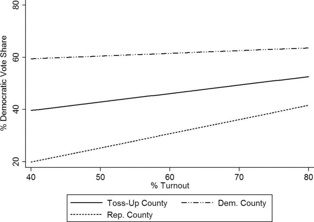
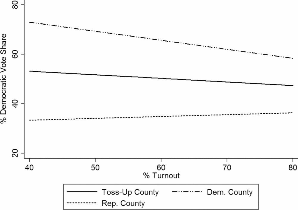
As a further illustration of the results of the IV model, we plot predicted Democratic vote share by turnout. In Figures 4 and 5, three sets of predicted vote shares are presented: one for “toss-up” counties (partisan composition is 50% Democratic), one for Republican counties (partisan composition is 30% Democratic), and one for Democratic counties (partisan composition is 70% Democratic). The predicted vote shares in Figure 4 are generated with Republican incumbent set at one, whereas in Figure 5 the predictions are based on a Democratic incumbent.Footnote 29
Effect of Turnout and Partisan Composition on Predicted Democratic Vote Share (Republican Incumbent)

Effect of Turnout and Partisan Composition on Predicted Democratic Vote Share (Democratic Incumbent)

These figures again reveal the conditional relationship between turnout and partisan vote share. When the incumbent president is a Republican, increases in turnout uniformly lead to a higher vote share for the Democratic candidate. The increase is steepest in Republican counties, and the slope becomes less steep as the size of the Democratic electorate increases. Given a Democratic incumbent, the direction of the effect of turnout depends on the partisan composition of the county. Increases in turnout in Democratic counties help the Republican candidate, whereas increases in Republican counties assist the Democratic candidate; however, as noted previously, this latter effect is not statistically different from zero. In toss-up counties, the model shows that high levels of turnout work against the Democrats.
Our IV results provide considerable support for all three hypotheses tested thus far. When we look at values of partisan composition and the partisanship of the incumbent president that lead to statistically significant turnout effects, we find a significant pro-Democratic effect in 45% of the observations (county election dyads) in our data and a significant pro-Republican effect in only 2% of the observations. We can therefore state that when there is a significant turnout effect, it is generally pro-Democratic. This result is compatible with the Partisan Effect Hypothesis.Footnote 30 Our analysis also supports the Two-Effects Hypothesis. Although increases in turnout more often help the Democratic candidate than the Republican candidate, the effect of turnout is clearly conditioned by the partisan composition of an electorate (a county, in our data). There is also clear evidence of an anti-incumbent effect at work. This is demonstrated by the fact that turnout exerts a statistically significant and positive effect on Democratic vote share for 95% of the observations in our data in which there is a Republican incumbent. When there is a Democratic incumbent, turnout never exerts a positive, significant pro-Democratic effect, regardless of the partisan composition of a county.Footnote 31 The only significant effect that turnout has in this scenario is a pro-Republican effect in very Democratic counties. In sum, increases in turnout captured by our instrument exert three effects: pro-Democratic, antimajority party in the electorate, and anti-incumbent.Footnote 32
Spatial Autocorrelation
We have been careful to account for election- and county-specific effects with our inclusion of fixed effects for each. In fact, the county fixed effects also account for any state effects that are constant over time because the county effects are simply disaggregated state effects. Yet it is possible that there are state-election dyadic-specific effects that are unaccounted for in our model and thus lead to spatial autocorrelation, meaning that the residuals for the counties in a given state in a given election year might not be independent from each other. Furthermore, as illustrated in Figure 1, our instrument, election day rainfall, is not randomly distributed across counties in a given election. Neighboring counties are likely to experience similar weather on any given day, and thus our instrument naturally exhibits spatial correlation. Consequently, despite the fact that we have 27,401 county elections in our data, there is a danger that a few regionally concentrated storms are influencing our results. This concern is heightened by the fact that if we exclude from our analysis the two rainiest elections (1992 and 2000), our instrument loses power, our model identification suffers, and the two key coefficient estimates are no longer statistically significant (p = .089 and .093 with one-tailed tests, for turnout × partisan composition and turnout × Republican incumbent, respectively), although each is in the hypothesized direction and actually increases in magnitude.Footnote 33 It is important to note, however, that if we exclude either 1992 or 2000, the IV model is sufficiently identified, and the estimates for these two interaction terms are statistically significant and in the same direction as the results reported in Table 1.
An analysis of the residuals from our IV model reveals that they are not fully independent for the counties in a given state in a given election—in other words, the residuals are spatially correlated.Footnote 34 In general, there are a few possible ways to address the issue of spatial autocorrelation, although the IV context makes dealing with this problem a bit more complicated due to identification concerns. One straightforward solution to any potential correlation of residuals for counties within a given state for a given election is to include state-election fixed effects (e.g., a fixed effect for California in 1948, California in 1952, etc.) in our IV model. Unfortunately, diagnostics indicate that our IV model is no longer sufficiently identified when these additional fixed effects are included. These state-election effects reduce the explanatory power of our instrument in the first-stage models because rainfall (or its absence) on any election day will be geographically clustered.Footnote 35 Even with the additional state-election fixed effects, the second-stage model results are somewhat consistent with the results presented in Table 1 because turnout × Republican incumbent has a positive and significant coefficient (1.29, p = .011), whereas turnout × partisan composition has a negative and insignificant coefficient (−.005, p = .163). These particular results must be treated with caution, however, due to the lack of sufficient identification. It is possible that the identification problems we experience due to the inclusion of these additional fixed effects is further evidence that spatial autocorrelation is a concern here.
A common way to address the effect that spatial autocorrelation can have on the estimates of standard errors is to estimate robust standard errors that “cluster” on the grouping variable in question. However, clustering is not straightforward when the grouping variable (state-election dyad) is different from the panel variable (county), which is our situation.Footnote 36 Nonetheless, when these clustered standard errors are estimated, they are substantially larger than the robust standard errors that do not cluster on state-elections, and these larger standard errors would cause us to fail to reject the null hypotheses for all key independent variables in the model (and all but two of the election dummy variables). We are skeptical about the size of these standard error estimates, though. These clustered standard errors are just as large, if not larger, when they are clustered on states, instead of state-elections, despite the fact there is no correlation of residuals within states (as compared to state-elections).
To attempt a blunt test of the consequences of spatial autocorrelation in our data, we aggregate our data to the state level (reducing our N from 27,401 to 517). By definition, these data cannot suffer from state-election spatial autocorrelation because there is only one observation for each state in each election. This higher level of aggregation leads to insufficient identification for the two interaction terms in our model, but the constituent turnout variable is sufficiently identified to estimate an IV model of state-level Democratic vote share. In this model estimation, the effect of turnout is positive and statistically significant, which is reassuringly consistent with the average effect of turnout in the IV models presented in the second column of Table 1.
For our final and we believe most compelling effort to address the nonindependence of residuals for counties in a given state and election year, we attempt to directly control for various potential sources of spatial autocorrelation by including a wide variety of independent variables that should soak up much of the state-election effects. We identify and include four such types of variable: state laws regarding registration/voting, statewide elections occurring at the same time as the presidential election, expected closeness of the state in the presidential election, and candidate connections to the state.Footnote 37 These variables might affect turnout and/or vote shares within a state in a particular election.
With these state-election–specific variables in place, we re-estimate our IV model (still including county fixed effects and election fixed effects), and the results for the variables of interest are presented in the final column of Table 1. An analysis of the residuals for this model reveals that the inclusion of these controls reduces, but does not eliminate, the spatial autocorrelation.Footnote 38 After this reduction in spatial autocorrelation, the IV results remain robust, which gives us confidence that spatial autocorrelation is not driving our results. For the rest of the article, we use the IV results obtained without the inclusion of these additional state-election variables because there may be endogeneity concerns with some of the variables in the saturated model (e.g., registration requirements might be endogenous to vote shares). Furthermore, the results for the more parsimonious model are somewhat more conservative in the sense that the conditional effects of turnout are smaller in magnitude.
Implications for the Aggregate Behavior of Marginal Voters
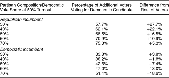
To gain further information from our IV results, we use the estimates presented in the second column of Table 1 (i.e., those without the state-election controls) to simulate the voting patterns of the marginal voters who may or may not vote in a given election. For purposes of illustration, we base our simulation on a hypothetical county in which the baseline turnout is 50%. Although varying both the partisan identification of the incumbent president and the partisan composition of the county, we use our IV estimates to predict the change in Democratic vote share based on a one percentage point increase in turnout (i.e., increasing turnout from 50% to 51%). Using this predicted change and some basic algebra, we then determine how this additional one percentage point worth of voters (i.e., marginal voters) voted. Table 2 presents these predicted Democratic vote shares for these marginal voters.
Inferred Voting Patterns of Marginal Voters When a County's Turnout Increases from 50% to 51%
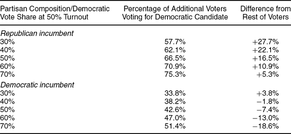
Notes: These vote shares are calculated based on the IV results presented in column 2 of Table 1. For these calculations, the baseline turnout is set at 50%, and the baseline Democratic vote share is set equal to partisan composition (e.g., a partisan composition of 60% Democratic equals a baseline vote share of 60% Democratic).
The second column of Table 2 contains the simulated percentage of the additional marginal voters voting for the Democratic candidate. The third column contains the difference between this vote share for the marginal voters and the vote share for the “core” 50% who turned out (which, for the sake of simplicity, is assumed to be equal to the partisan composition of the county; i.e., percentage Democratic). This simulation reveals that when the partisan, antimajority, and anti-incumbent effects work together, there is a marked difference between the voting patterns of the marginal voters and the core voters, as we have defined them here. Specifically, when the hypothetical county is highly Republican (only 30% Democratic) and there is a Republican incumbent, the vote share for the marginal voters is nearly 28 percentage points more Democratic than that of the core voters. Typically, however, these three effects will not work together to this extent, and thus, the differences in the aggregate voting behavior of core and peripheral voters are usually smaller, although often still quite impressive.
Several survey-based studies compare the vote choice of actual voters with predicted vote choices of nonvoters. While these studies typically conclude that changes in voter turnout would only occasionally affect election outcomes, they do report substantial differences in the vote choices of voters and the predicted or self-reported likely votes of nonvoters. For example, from Highton and Wolfinger's (Reference Highton and Wolfinger2001) results, it can be derived that, in 1996, Clinton's two-party vote share would have been 22.3 percentage points greater with nonvoters than voters. Teixeira (Reference Teixeira1992, 96) examines several earlier presidential elections and finds that nonvoters range from reporting likely vote shares that are somewhat disproportionately Republican in the 1980s to reporting likely vote shares that are more than 12 percentage points more Democratic than actual voters in 1964. In their survey-based examination of the likely votes of nonvoters in Senate elections, Citrin, Schickler, and Sides (Reference Citrin, Schickler and Sides2003) find that the difference in the vote shares of voters and nonvoters ranged from approximately 10 percentage points more for the Democratic candidate to 5 percentage points more for the Republican. As these studies reveal, the vote share swings we report in Table 2 are not wildly out of line with those obtained by surveys, even though some of the swings are quite dramatic. The advantage to our simulations over the survey-based studies is that the surveys take place after the election and, as Campbell et al. (Reference Campbell, Converse, Miller and Stokes1960, 112) speculate, nonvoters with weak partisan ties are likely to simply report that they would have voted for the winner of the election. Furthermore, we use a large number of elections while controlling for election-specific effects. The survey-based studies tend to rely on data from a small number of elections, which makes it more difficult to separate out general turnout effects from election-specific influences.
How Meaningful Are Turnout Effects at the Aggregate Level?
Do our county-level results translate into important turnout effects at higher levels of aggregation? To address this question, we use the results of our IV model (without state-election controls) to predict for each election how Democratic vote share would have changed in each non-Southern county based on changes from the actual, observed level of turnout in the county. Note that the effect of a change in turnout in each county depends on the partisan composition of the county and the party of the incumbent president. Weighting each county by its number of voters, we then aggregate these predicted changes in vote share to determine the effect of uniform changes in turnout. These effects are aggregated at both the national level and the state level. The former reveals the estimated effect of turnout on national vote share (excluding the South), whereas the latter is used to estimate the effect of turnout on Electoral College outcomes.
Through this aggregation process, we find that our county-level effects have implications at the national level. We simulate the change in national Democratic vote share based on a four percentage point swing in turnout (i.e., ranging turnout from two percentage points below the actual turnout for the election to two percentage points above). Note that a four percentage point variation in turnout is not unreasonable, and may be viewed as conservative, given that national-level turnout has a much greater range than this over our 14 elections (ranging from 49.1% to 63.3%). Furthermore, prior research suggests that simple changes to voter registration requirements, for instance, could lead to changes in national-level turnout that exceed four percentage points (e.g., Rosenstone and Wolfinger Reference Rosenstone and Wolfinger1978). In his meta-analysis of aggregate-level turnout studies, Geys (Reference Geys2006) finds that a one standard deviation increase in the closeness of an election leads to more than half of a standard deviation increase in turnout. Again, our hypothetical variation in turnout appears to be on the conservative side, given that Gey's result implies that moving from one standard deviation below the mean closeness of an election to one standard deviation above mean closeness would lead to more than a four percentage point swing in turnout (which has a standard deviation of 4.9% at the national level during our time span). Based on our simulation, we find that a 4% swing in turnout leads to an average change in Democratic vote share at the national level of just less than one percentage point.Footnote 39
When we aggregate our results to the state level, we find that varying turnout from two points above and below observed values causes an average change of approximately 20 Electoral College votes per election. In fact, in the 1948, 1960, and 1976 elections, at least 50 Electoral College votes change. These are not trivial effects, especially considering that they exclude the Electoral College votes of Southern states. Although election-specific factors other than turnout have the greatest effect on who wins an election (Kaufman, Petrocik, and Shaw Reference Kaufman, Petrocik and Shaw2008, 147), it appears that variation in turnout, at least the sort captured by our IV approach, can exert an effect on vote shares at the county, national, and Electoral College level.
Testing the Volatility Hypothesis
The IV results presented in Table 1 suggest that high turnout elections are likely to have negative electoral consequences for the majority party in an electorate and for the incumbent party in the White House. As such, high turnout elections may be quite disruptive. Our Volatility Hypothesis builds on this underlying logic and asserts that increases in turnout should lead to less predictable (i.e., more volatile) vote shares. By bringing nontraditional voters into the electorate, the electoral outcomes of high turnout elections should be more variable. To test this proposition, we use the predictability of Democratic vote share as the dependent variable in our final analysis. To measure this, we calculate the residuals from the IV model without state-election controls (presented in the second column of results in Table 1) and then square them. A large squared residual indicates a county election dyad for which our model in Table 1 does a poor job of predicting Democratic vote share. Small squared residuals are associated with more predictable data points.Footnote 40
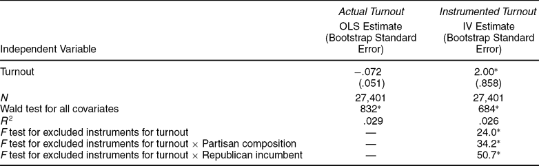
We again use the IV approach and regress these squared residuals on instrumented turnout, as well as the county- and election-specific fixed effects.Footnote 41 Because our dependent variable and key independent variable are predicted values, traditional standard errors cannot be used (Pagan Reference Pagan1984). We therefore bootstrap the standard errors associated with the coefficient estimates (Mooney and Duval Reference Mooney and Duval1993). These results are presented in Table 3.
Volatility in County-level Democratic Vote Share in Presidential Elections, 1948–2000
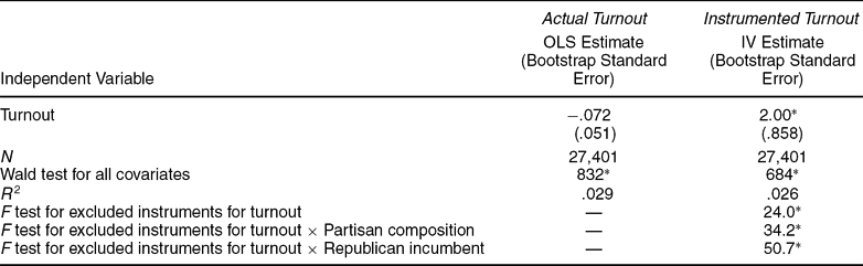
Notes: The dependent variable for the OLS model is the squared residuals from the OLS model presented in Table 1. The dependent variable for the IV model is the squared residuals from the IV model without the state-election controls presented in Table 1. Fixed effects for counties and for election years are included in the model. Southern counties are excluded from the analysis.
* p ≤ .05 (one-tailed test).
As suggested by the Volatility Hypothesis, the coefficient estimate for instrumented turnout is positive and statistically significant. Increases in turnout cause larger residuals in our full vote share model. In other words, increases in turnout make the two-party vote share less predictable at the county level. As turnout increases in a county, the fixed effect for the county (the county-specific constant), the partisan composition of the county, the fixed effect for the election (the national election-specific constant), and, ironically, the turnout variable itself lose some power to explain Democratic vote share. For a given presidential election, counties with higher turnout will deviate more from the national trend (captured by the election-specific fixed effect) in that election, all else equal. For a given county, high turnout elections are associated with a greater deviation from the mean Democratic vote share exhibited by that county over the latter half of the twentieth century.
In sum, these results imply that the irregular voters who contribute to high turnout event are less predictable than regular voters. When these peripheral voters do turn out, aggregate vote shares become less predictable. Importantly, the electoral volatility caused by increases in turnout is not detected by the standard approaches to this problem. The OLS estimate obtained with actual turnout is not statistically distinguishable from zero, suggesting that models that do not account for the endogenous relationship between turnout and vote share are unlikely to reveal the electoral volatility caused by higher turnout.
CONCLUSION
Political scientists have long pondered the electoral consequences of voter turnout. Most have presumed that in the United States, turnout serves as a lever for the electoral fortunes of the Democratic Party. The conventional wisdom is that Democratic vote share rises with turnout, owing to an infusion of atypical voters—who tend to share a demographic profile with traditional Democratic voters—into the electorate. Yet the empirical evidence regarding the partisan consequences of turnout has been far from incontrovertible. Moreover, few scholars have looked beyond the partisan implications to examine the effect of high turnout on incumbency or electoral volatility in general. Our novel approach to testing the electoral implications of variation in voter turnout yields two central contributions.
First, we make a theoretical case for the endogenous relationship between turnout and vote choice. We then demonstrate empirically that aggregate turnout and aggregate electoral outcomes are endogenous. The fact that previous research has not accounted methodologically for this endogeneity strikes us as surprising. After all, most observers recognize that voters sometimes choose for whom they want to vote before they actually decide whether to turn out to vote. This is true, for instance, whenever it is asserted that an emergent, perhaps charismatic, candidate is likely to bring new voters to the polls. It is also the case when a nonvoter decides to abstain because he or she perceives the choice as being a regrettable selection between Tweedledum and Tweedledee.Footnote 42 In cases such as these, or more axiomatically in Downs's calculus of voting, the vote choice is conceived as preceding the decision to go to the polls. By not accounting for the potential endogeneity in the relationship between turnout and electoral outcomes, the causal claims made in previous studies must be treated with some skepticism.
Second, by leveraging a unique instrument for voter turnout, we are able to pin down the causal effect of much of the variation in voter turnout on electoral outcomes. As such, we believe that we provide the strongest and clearest evidence to date of the political importance of variation in turnout, at least variation of the sort captured by our instrument. Our empirical results present a more complex, nuanced view of the effect of turnout on presidential elections. We show “four effects” to be at work. Democratic candidates, on average, are helped by higher turnout. The partisan composition of the electorate and the party of the incumbent president condition this relationship, however. Furthermore, we show that higher turnout results in greater levels of electoral volatility more generally.
In low turnout elections, where the electorate is comprised primarily of core voters who possess relatively strong and unwavering partisan attachments, electoral outcomes reflect this underlying stability. Low turnout elections tend to benefit Republican candidates on average, a by-product of the GOP's relative advantage with core voters, who tend to be of a higher socioeconomic status than peripheral voters. Our results also indicate that low turnout tends to validate the status quo because elections of this type significantly advantage the party of the incumbent president. Combined, these results suggest that the voters in low turnout elections are likely to exert little “change” when they go to the polls. Put differently, lower levels of turnout may yield representational bias in the electoral connection. Interestingly, this bias is not simply partisan in nature because low turnout also produces a proincumbent bias.
High turnout elections, in contrast, bring both core and peripheral voters to the polls. Importantly, the infusion of this latter group into the electorate may contribute to outcomes that are both potentially disruptive to the existing political order and less systematically predictable. Peripheral voters are likely to possess weak partisan or ideological attachments at best and thus are more influenced by transient or idiosyncratic considerations. It appears the infusion of these atypical or peripheral voters into the electorate has consequences for America's political parties. Our findings conform to those hypothesized by DeNardo's Two-Effects thesis. That is, although higher turnout benefits Democrats on average, the magnitude of those benefits is conditioned by the composition of the electorate being brought to the polls. Indeed, in highly Democratic electorates, high turnout may actually help the Republicans, who benefit from weak partisans defecting from their Democratic attachments. In addition to these partisan effects, we find that high turnout also has a significant anti-incumbency effect. Peripheral voters not only have weak partisan ties, but they may also be less likely to support the electoral status quo. Consequently, when the electorate expands with these voters, the incumbent party is fighting an uphill battle. Compared to their more participatory counterparts, infrequent voters bring both change and noise when they go to the polls. High turnout elections portend partisan change, anti-incumbency tendencies, and generally less predictable consequences.
APPENDIX
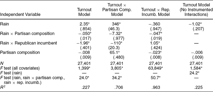
The IV models presented in Table 1 treat three independent variables as endogenous: turnout, turnout × partisan composition, and turnout × Republican incumbent. There are thus three first-stage models, one for each endogenous variable. Following IV convention, each first-stage model includes all three excluded instruments: rain, rain × partisan composition, and rain × Republican incumbent. The first-stage estimates for the model without state-election controls are presented in the first three columns of Table A1.Footnote 43
First-stage Results: Predicting County-level Turnout, 1948–2000
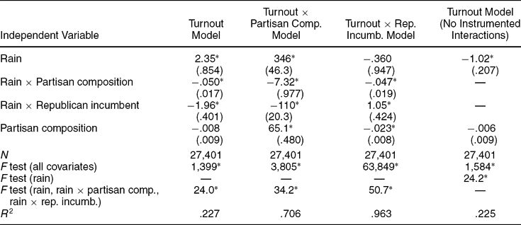
Notes: Cell entries are coefficient estimates (robust standard errors). Fixed effects for county and for election year are included in all models. Southern counties are excluded from the analysis.
*p ≤ .05 (two-tailed test).
These estimates imply that the effect of rain on turnout is conditioned by Republican incumbent and partisan composition. Note that despite the positive “main effect” for rain in the turnout model, the average conditional effect of rain on turnout is negative (−.85, based on the average values of conditioning variables). The key considerations when determining whether rainfall is a valid instrument for turnout are (1) exogeneity and (2) explanatory power. We believe that it is safe to assume that rainfall is exogenous to vote choice, so we will not belabor the point. Does it have enough explanatory power? The econometric rule of thumb is that an F statistic of 10 or greater indicates that an instrument (or set of instruments) has sufficient explanatory power for IV estimation (Staiger and Stock Reference Staiger and Stock1997). As reported in Tables 1 and A1, our rainfall variable and associated interaction terms far exceed this threshold.
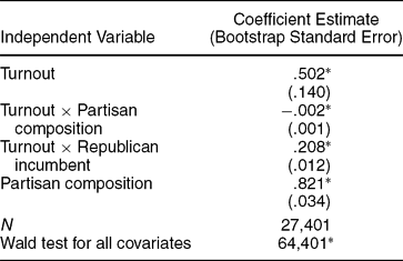
To ensure that the conditional effect of rain on turnout in the first stage of the IV model is not problematic for the estimation of the main model, we re-estimate the IV model while employing a somewhat different strategy. We predict just turnout in the first stage while including rain as instrument and excluding the interaction terms involving rain. The results of this alternative first stage are reported in the last column of Table A1. Then, we multiply predicted turnout with Republican incumbent and partisan composition, and include these interactions in the main model. This approach forces rain to have a constant, nonconditional effect on turnout in the first stage. One disadvantage to this approach is that the estimated standard errors may not be correct in the second stage, but this can be resolved by bootstrapping these second-stage standard errors. The results obtained by this alternative IV strategy are presented in Table A2. These results are quite similar to those presented in Table 1, and the fundamental inferences are the same. This indicates that allowing the effect of rain on turnout in the first stage to be conditional is not determinative of the ultimate conclusions drawn based on the second-stage model of vote shares.
Alternative IV Approach to Modeling County-level Democratic Vote Share in Presidential Elections, 1948–2000
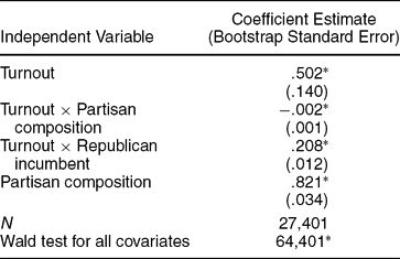
Notes: The model includes fixed effects for county and for election year. Southern counties are excluded from the analysis. The standard errors are bootstrapped (500 repetitions).
*p ≤ .05 (one-tailed test).
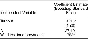
We then square the residuals from the model presented in Table A2 and regress them on the alternative version of predicted turnout to retest our Volatility Hypothesis. These results are presented in Table A3. The result is fundamentally similar to that presented in Table 2. Both IV strategies lead to the conclusion that increases in voter turnout cause greater volatility in presidential vote shares.
Alternative IV Approach to Modeling Volatility in County-level Democratic Vote Share in Presidential Elections, 1948–2000

Notes: The dependent variable is the squared residuals from the model presented in Table A2. Fixed effects for counties and for election years are included in the model. Southern counties are excluded from the analysis.
* p ≤ .05 (one-tailed test).



Comments
No Comments have been published for this article.