2 Problem formulation and computational details

In accordance with our prior studies of polymer-induced turbulent drag reduction (Li, Sureshkumar & Khomami Reference Li, Sureshkumar and Khomami2006; Liu & Khomami Reference Liu and Khomami2013a ,Reference Liu and Khomami b ; Li et al. Reference Li, Sureshkumar and Khomami2015), the FENE-P (finitely extensible nonlinear elastic-Peterlin) constitutive equation is used to model the polymer contribution to total stress. We have chosen $h$ , $h/U_{w}$ , $U_{w}$ and $\unicode[STIX]{x1D70C}U_{w}^{2}$ as scales for length, time, velocity $\boldsymbol{u}$ and pressure $p$ , respectively. Here $h$ denotes the half-height of the channel, $U_{w}$ represents the wall translation velocity and $\unicode[STIX]{x1D70C}$ denotes the solution density. Further, we scale the conformation tensor $\unicode[STIX]{x1D63E}$ , which represents the ensemble average of the second moment of the end-to-end vector of the polymer chains, with respect to $kT/H$ , where $k$ , $T$ and $H$ denote the Boltzmann constant, absolute temperature and Hookean spring constant of the elastic dumbbell model, respectively. The resulting dimensionless equations governing the motion of an incompressible FENE-P fluid are as follows:

(2.1) $$\begin{eqnarray}\displaystyle & \displaystyle {\displaystyle \frac{\unicode[STIX]{x2202}\boldsymbol{u}}{\unicode[STIX]{x2202}t}}+\boldsymbol{u}\boldsymbol{\cdot }\unicode[STIX]{x1D735}\boldsymbol{u}=-\unicode[STIX]{x1D735}P+{\displaystyle \frac{1}{Re}}\unicode[STIX]{x1D6FB}^{2}\boldsymbol{u}+\unicode[STIX]{x1D735}\boldsymbol{\cdot }\unicode[STIX]{x1D749}^{p} & \displaystyle\end{eqnarray}$$

and

(2.2) $$\begin{eqnarray}\displaystyle & \displaystyle {\displaystyle \frac{\unicode[STIX]{x2202}\unicode[STIX]{x1D63E}}{\unicode[STIX]{x2202}t}}=-\boldsymbol{u}\boldsymbol{\cdot }\unicode[STIX]{x1D735}\unicode[STIX]{x1D63E}+\unicode[STIX]{x1D63E}\boldsymbol{\cdot }\unicode[STIX]{x1D735}\boldsymbol{u}+(\unicode[STIX]{x1D735}\boldsymbol{u})^{\text{T}}\boldsymbol{\cdot }\unicode[STIX]{x1D63E}-\unicode[STIX]{x1D749}^{p}. & \displaystyle\end{eqnarray}$$

The polymer stress tensor $\unicode[STIX]{x1D749}^{p}$ is obtained as

(2.3) $$\begin{eqnarray}\displaystyle & \displaystyle \unicode[STIX]{x1D749}^{p}={\displaystyle \frac{1-\unicode[STIX]{x1D6FD}}{\unicode[STIX]{x1D6FD}}}{\displaystyle \frac{1}{ReWe}}\left({\displaystyle \frac{L^{2}-3}{L^{2}-\text{trace}(\unicode[STIX]{x1D63E})}}\unicode[STIX]{x1D63E}-\unicode[STIX]{x1D644}\right), & \displaystyle\end{eqnarray}$$

where $\unicode[STIX]{x1D6FD}=\unicode[STIX]{x1D702}_{s}/\unicode[STIX]{x1D702}_{t}$ , with $\unicode[STIX]{x1D702}_{s}$ and $\unicode[STIX]{x1D702}_{p}$ being respectively the solvent and polymeric contributions to the total viscosity $\unicode[STIX]{x1D702}_{t}$ , $L$ is the maximum chain extensibility; the Weissenberg number is defined as $We=\unicode[STIX]{x1D706}U_{w}/h$ (the ratio of the elastic relaxation time $\unicode[STIX]{x1D706}$ relative to the flow time scale $h/U_{w}$ ) and the Reynolds number as $Re=\unicode[STIX]{x1D70C}U_{w}h/\unicode[STIX]{x1D702}_{s}$ . A fully spectral, three-dimensional parallel algorithm (Li et al. Reference Li, Sureshkumar and Khomami2006, Reference Li, Sureshkumar and Khomami2015; Liu & Khomami Reference Liu and Khomami2013a ,Reference Liu and Khomami b ; Teng et al. Reference Teng, Liu, Lu and Khomami2015) is employed to solve the governing equations, i.e. Chebyshev polynomials in the wall-normal ( $y$ -) direction and Fourier series in the streamwise ( $x$ -) and spanwise ( $z$ -) directions. These equations are also supplemented by the no-slip boundary conditions at the walls, as well as periodic boundary conditions in the $x$ - and $z$ - directions. The initial condition is a fully developed turbulent Newtonian PCF with introduction of a unit conformation tensor (Nguyen et al. Reference Nguyen, Delache, Simoens, Bos and Hajem2016; Pereira et al. Reference Pereira, Mompean, Thais and Soares2017a ,Reference Pereira, Mompean, Thais, Soares and Thompson b ).

In addition, a diffusive term $\unicode[STIX]{x1D705}\unicode[STIX]{x1D6FB}^{2}\unicode[STIX]{x1D63E}$ is added to equation (2.2) in the bulk flow region to numerically stabilize the integration of the conformation tensor evolution equation. In order to retain the essential dynamics resulting from flow–microstructure coupling while maintaining numerical stability, the value of the scalar stress diffusivity $\unicode[STIX]{x1D705}$ should be chosen to be as low as possible (Li et al. Reference Li, Sureshkumar and Khomami2006). In the present study, a $\unicode[STIX]{x1D705}$ value corresponding to a Schmidt number of $Sc=1/(\unicode[STIX]{x1D705}Re)=0.15$ is used for all the calculations. This Schmidt number is of the same order as the values used by Li et al. (Reference Li, Sureshkumar and Khomami2006) and Thais et al. (Reference Thais, Gatskid and Mompeana2012). Note that the original constitutive equation without the diffusive term is applied at the walls, thus no boundary conditions are imposed at the walls for $\unicode[STIX]{x1D63E}$ .

In the present study, the Reynolds number is fixed at 1300 (Komminaho et al. Reference Komminaho, Lundbladh and Johansson1996; Tsukahara et al. Reference Tsukahara, Kawamura and Shingai2006), and the Weissenberg number is varied from 0 to 7, corresponding to a low elasticity number, i.e. $E=We/Re=0{-}0.005$ . We use a large value of $L=120$ and $\unicode[STIX]{x1D6FD}=0.9$ in that the polymeric solution has a nearly shear-independent viscosity (Li et al. Reference Li, Sureshkumar and Khomami2006, Reference Li, Sureshkumar and Khomami2015; Liu & Khomami Reference Liu and Khomami2013a ,Reference Liu and Khomami b ). To capture the LSSs in the core region, a much larger computational domain is necessary for PCF as compared to PPF (Komminaho et al. Reference Komminaho, Lundbladh and Johansson1996; Tsukahara et al. Reference Tsukahara, Kawamura and Shingai2006; Avsarkisov et al. Reference Avsarkisov, Hoyas, Oberlack and García-Galache2014). Based on extensive test calculations, the computational domain is set as $L_{x}\times L_{y}\times L_{z}=40\unicode[STIX]{x03C0}\times 2\times 6\unicode[STIX]{x03C0}$ for the streamwise, wall-normal and spanwise directions, respectively. This corresponds to a grid size of $1024\times 129\times 256$ . A time step of $\unicode[STIX]{x0394}t=0.01$ is used for the present calculations. Basically, our simulations have a mesh size 8 times larger than that of the drag-reduced PPF simulations conducted by Li et al. (Reference Li, Sureshkumar and Khomami2006, Reference Li, Sureshkumar and Khomami2015). This results in a significant increase in computational cost; hence, limiting the maximum $Re$ that DNS of drag-reduced PCF can access with today’s most powerful supercomputers.

Figure 1.

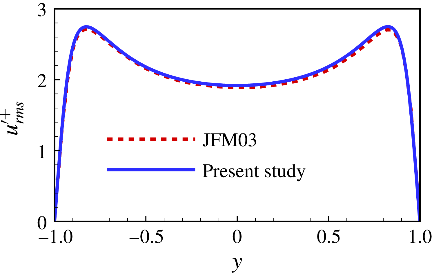
Comparison of root-mean-square (r.m.s.) value of streamwise velocity fluctuation with that obtained by Hu, Morfey & Sandham (Reference Hu, Morfey and Sandham2003). The superscript ‘+’ is hereafter used to denote the quantity non-dimensionalized by the viscous length scale $\unicode[STIX]{x1D6FF}=\unicode[STIX]{x1D708}_{s}/u_{\unicode[STIX]{x1D70F}}$ ; the friction velocity is defined as $u_{\unicode[STIX]{x1D70F}}=\sqrt{\unicode[STIX]{x1D70F}_{w}/\unicode[STIX]{x1D70C}}$ where $\unicode[STIX]{x1D70F}_{w}$ is the total wall stress; the overbar denotes ensemble averaging.

Figure 2.

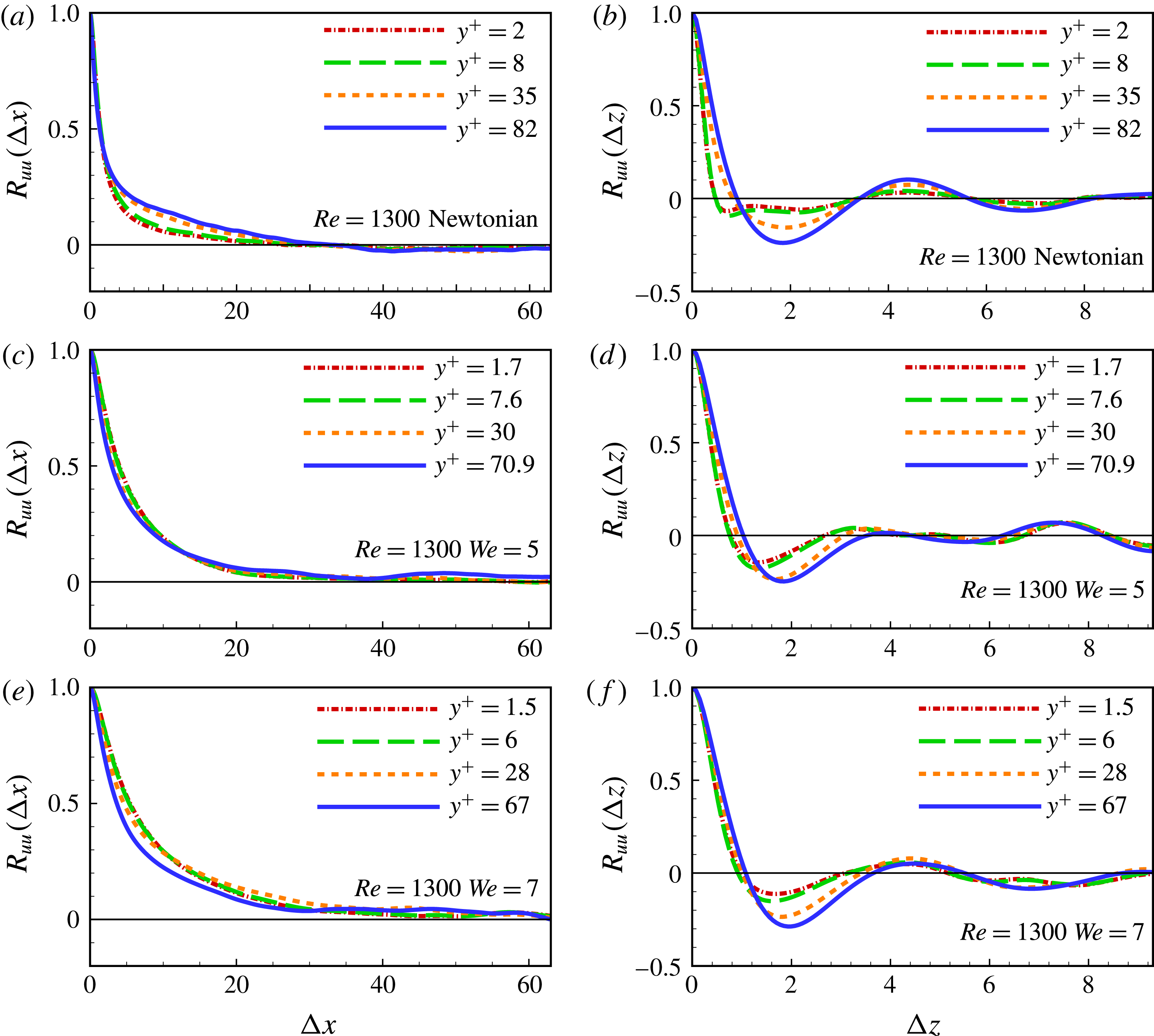
The two-point correlations of the streamwise velocity fluctuation for Newtonian PCF (a,b), and drag-reduced PCFs of $We=5$ (c,d) and $We=7$  (e,f).

The code used in the present study has been extensively validated and successfully used in previous simulations of drag-reduced PPF (Li et al. Reference Li, Sureshkumar and Khomami2006, Reference Li, Sureshkumar and Khomami2015). In the present work, code validation includes calculation of Newtonian PCF under the same conditions as the comprehensive study by Hu et al. (Reference Hu, Morfey and Sandham2003). All of our simulation results are in full agreement with the aforementioned study. Specifically, both the streamwise velocity fluctuations (see figure 1) and the scales of the coherent structures (see figure 2), namely, the streamwise and spanwise scales determined by two-point correlations $R_{uu}(\unicode[STIX]{x0394}x)$ and $R_{uu}(\unicode[STIX]{x0394}z)$ , show similar behaviour. The two-point correlations are defined as

(2.4) $$\begin{eqnarray}\displaystyle & \displaystyle R_{uu}(\unicode[STIX]{x0394}x)={\displaystyle \frac{\overline{u^{\prime }(x,z)u^{\prime }(x+\unicode[STIX]{x0394}x,z)}}{\overline{u^{\prime 2}}}} & \displaystyle\end{eqnarray}$$

and

(2.5) $$\begin{eqnarray}\displaystyle & \displaystyle R_{uu}(\unicode[STIX]{x0394}z)={\displaystyle \frac{\overline{u^{\prime }(x,z)u^{\prime }(x,z+\unicode[STIX]{x0394}z)}}{\overline{u^{\prime 2}}}}. & \displaystyle\end{eqnarray}$$

Hereafter, the superscript ‘ $\,^{\prime }\,$ ’ denotes the fluctuating part. As indicated in figure 2(a), the zero value of $R_{uu}(\unicode[STIX]{x0394}x)$ occurs at approximately 35 in the channel centre for Newtonian PCF, pointing to a streamwise scale of 70 for the large-scale coherent structures. This prediction is consistent with a value of $40\sim 65$ reported in prior studies (Tsukahara et al. Reference Tsukahara, Kawamura and Shingai2006; Avsarkisov et al. Reference Avsarkisov, Hoyas, Oberlack and García-Galache2014). The first minimum of $R_{uu}(\unicode[STIX]{x0394}z)$ for Newtonian PCF appears at approximately 0.73 (see figure 2 b) in the buffer layer $(y^{+}=8)$ . This corresponds to the spanwise scale of approximately 120 in wall units for near-wall coherent structures. This estimate is basically consistent with the well-accepted value of ${\sim}100$ in wall-bounded shear flows (Kline et al. Reference Kline, Reynolds, Schraub and Runstadler1967; Kim, Moin & Moser Reference Kim, Moin and Moser1987; Tiederman Reference Tiederman1990; Jiménez & Moin Reference Jiménez and Moin1991; Hamilton et al. Reference Hamilton, Kim and Waleffe1995; Tsukahara et al. Reference Tsukahara, Kawamura and Shingai2006; Monty et al. Reference Monty, Hutchins, Ng, Marusic and Chong2009). Note that PCF of low $Re$ , exhibits near-wall structures evidently influenced by the LSSs (Komminaho et al. Reference Komminaho, Lundbladh and Johansson1996). In consequence, the spanwise scale of near-wall coherent structures of 100 wall units is masked by the imprint effects of LSSs (Pizorroli et al. Reference Pizorroli, Bernardini and Orlandi2011); this phenomenon is discussed in detail in § 5.

Figure 2 also clearly demonstrates that in all of our calculations $R_{uu}(\unicode[STIX]{x0394}x)$ and $R_{uu}(\unicode[STIX]{x0394}z)$ decay to approximately zero at half of the domain size in the streamwise and spanwise directions. Hence, the computational domain used is sufficiently large to contain the LSSs appearing in the core region. In fact, to capture the scale enhancement due to drag reduction, the computational domain has been set larger than the previous DNS of Newtonian PCF (Avsarkisov et al. 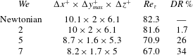Reference Avsarkisov, Hoyas, Oberlack and García-Galache2014). The precise values of key parameters in our simulations are provided in table 1.

Table 1.

Numerical parameters, where the friction Reynolds number is defined as $Re_{\unicode[STIX]{x1D70F}}=\unicode[STIX]{x1D70C}u_{\unicode[STIX]{x1D70F}}h/\unicode[STIX]{x1D702}_{s}$ .

3 Drag-reduction-related features in PCF

Similar to PPF, addition of flexible polymers can lead to drag reduction in PCF. As expected, the polymer-induced drag reduction is enhanced with the increase of $We$ (see table 1). The extent of drag reduction rate is computed as follows:

(3.1) $$\begin{eqnarray}\displaystyle & \displaystyle DR\,\%={\displaystyle \frac{\unicode[STIX]{x1D70F}_{w0}-\unicode[STIX]{x1D70F}_{w}}{\unicode[STIX]{x1D70F}_{w0}}}={\displaystyle \frac{Re_{\unicode[STIX]{x1D70F}0}^{2}-Re_{\unicode[STIX]{x1D70F}}^{2}}{Re_{\unicode[STIX]{x1D70F}0}^{2}}}, & \displaystyle\end{eqnarray}$$

where $\unicode[STIX]{x1D70F}_{w}=\unicode[STIX]{x1D70C}\unicode[STIX]{x1D708}_{s}(\text{d}\overline{u}/\text{d}y)+\overline{\unicode[STIX]{x1D70F}_{xy}^{p}}$ is the total wall stress, with $\overline{\unicode[STIX]{x1D70F}_{xy}^{p}}$ being the polymeric stress contribution. $\unicode[STIX]{x1D70F}_{w0}$ and $Re_{\unicode[STIX]{x1D70F}0}$ correspond respectively to the wall stress and the frictional Reynolds number of Newtonian PCF. It is found that $DR\,\%$ increases from $1.7\,\%$ to $26\,\%$ , then to $34\,\%$ when $We$ varies from 2 to 5, and then to 7 (see table 1). Hence, the drag reduction observed in PCF should be categorized as low drag reduction (LDR), namely, $DR\,\%<40\,\%$ (Dubief et al. Reference Dubief, White, Terrapon, Shaqfeh, Moin and Lele2004; White & Mungal Reference White and Mungal2008; Dallas et al. Reference Dallas, Vassilicos and Hewitt2010; Pereira et al. Reference Pereira, Mompean, Thais, Soares and Thompson2017b ).

Figure 3.

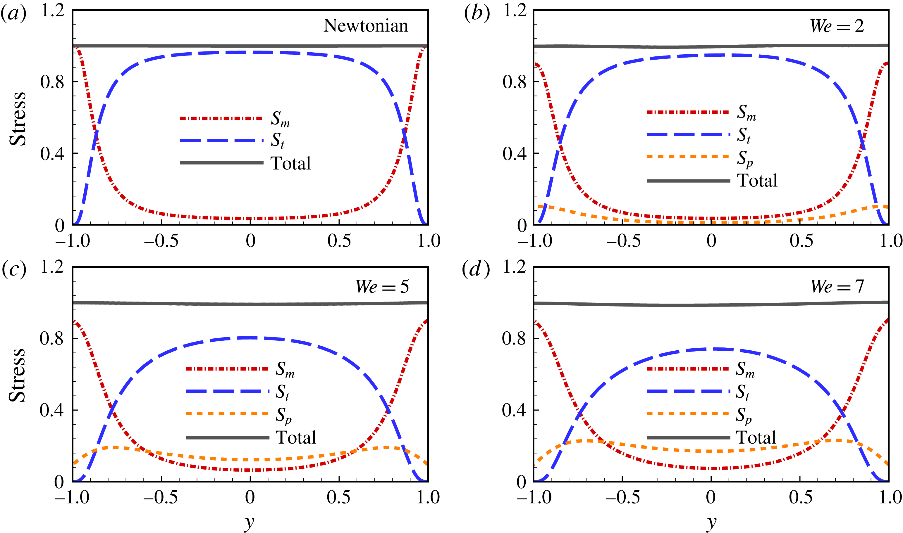
Overall force balance for Newtonian PCF (a), and drag-reduced PCFs with $We=2$ (b), $We=5$ (c) and $We=7$ (d).

A close examination of the overall force (or stress) is required to investigate the turbulence dynamics of drag-reduced flows. The force balance for drag-reduced PCF can be expressed as:

(3.2) $$\begin{eqnarray}\displaystyle & \displaystyle {\displaystyle \frac{\text{d}\overline{u}^{\,+}}{\text{d}y^{+}}}-\overline{u^{\prime }v^{\prime }}^{\,+}+\overline{\unicode[STIX]{x1D70F}_{xy}^{p}}^{\,+}=1, & \displaystyle\end{eqnarray}$$

where $\overline{u}^{\,+}$ is the mean flow velocity in wall units. The left-hand-side terms of equation (3.2) are in sequence: the shear stress $S_{m}=\text{d}\overline{u}^{\,+}/\text{d}y^{+}$ coming from mean flow shear, the Reynolds stress $S_{t}=-\overline{u^{\prime }v^{\prime }}^{\,+}$ accounting for turbulent momentum transfer and the polymer stress $S_{p}=\overline{\unicode[STIX]{x1D70F}_{xy}^{p}}^{\,+}$ , which vanishes for Newtonian PCF.

Clearly, an overall force balance is achieved in all the calculations; the total stress (i.e. the sum of the shear stress $S_{m}$ , the Reynolds stress $S_{t}$ and the polymer stress  $S_{p}$ ) is equal to unity over the entire channel (see figure 3). This clearly demonstrates that fully stationary states have been realized. Similar to PPF (Li et al. Reference Li, Sureshkumar and Khomami2006, Reference Li, Sureshkumar and Khomami2015), the Reynolds stress has a dominant contribution in the core region for the Newtonian case – approximately 90 % of the total stress. As $We$ is increased, $S_{t}$ decreases continuously and reaches a value of less than 80 % of the total stress. This indicates that polymer additives reduce turbulent momentum transfer. On the other hand, a substantial enhancement of polymer stress is observed when $We$ increases from 0 to 7. Specifically, for $We=7$ , $S_{p}$ contributes approximately 20 % to the total stress in the core region. Moreover, a non-zero $S_{m}$ value occurs at the channel centre and becomes greater, indicating a growth of mean flow shear with the increase of $We$ . Thus, the polymer stress and the mean flow shear are expected to have major effects on the bulk flow of drag-reduced PCF.

Figure 4.

Mean streamwise velocity $\overline{u}$ profile across the channel (a) and its log plot in the lower half of the channel versus the wall-normal distance (b), here $\overline{u}^{+}\equiv (\overline{u}+U_{w})^{+}$ . The log law corresponds to $\overline{u}^{+}=(1/k)\text{ln}(y^{+})+C$ with $k=0.41$ and $C=5.1$ (Avsarkisov et al. Reference Avsarkisov, Hoyas, Oberlack and García-Galache2014) and Virk law corresponds to $\overline{u}^{+}=11.7\,\text{ln}(y^{+})-17$ (Virk Reference Virk1975).

Figure 5.

Profiles of r.m.s. values of streamwise (a), wall-normal (b) and spanwise (c) velocity fluctuations, and turbulent kinetic energy (d).

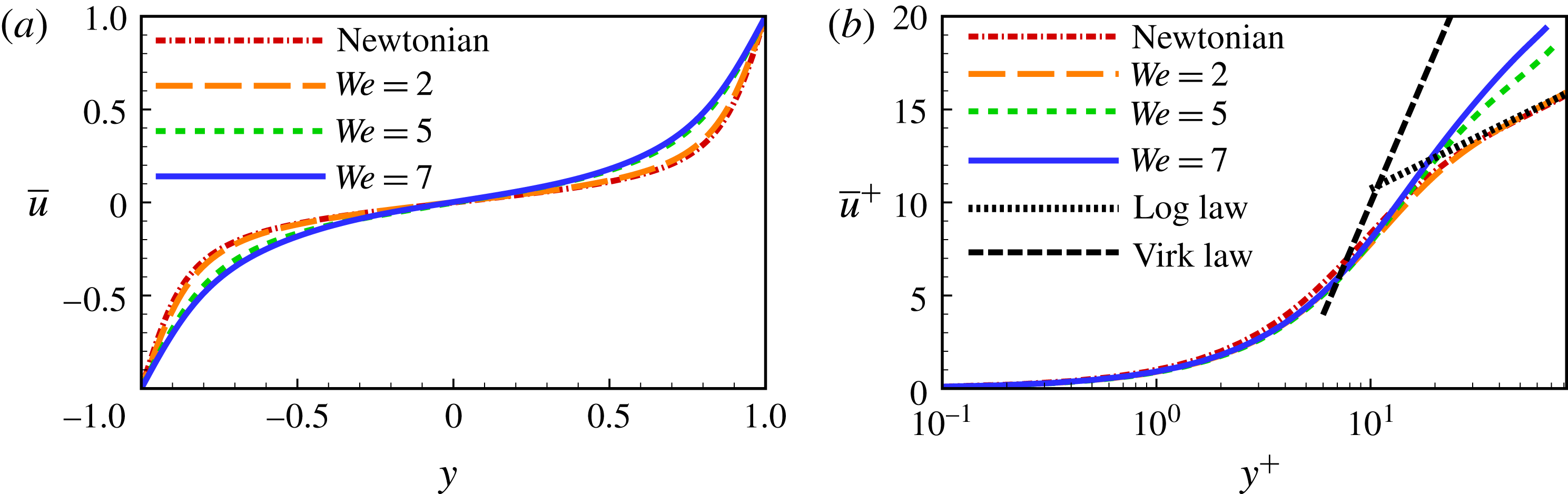
The flow response to the addition of polymer is examined (see figure 4) by observing the changes in the mean flow velocity $\overline{u}$ . Specifically, the gradient of mean flow velocity decreases at the wall with a commensurate decrease in wall shear stress (see figure 4 a). In contrast, in the core region the $\overline{u}$ gradient increases, pointing to an enhanced $S_{m}$ , as shown in figure 3. Figure 4(b) presents the log plot of $\overline{u}^{\,+}$ for different $We$ . It has been demonstrated that the mean flow velocity collapses into the classical log law in the outer region for Newtonian PCF (Avsarkisov et al. Reference Avsarkisov, Hoyas, Oberlack and García-Galache2014). As $We$ is increased from 0 to 7, $\overline{u}^{\,+}$ increases in the outer region, resulting in a deviation from the log law while trending towards the well-known Virk law (Virk Reference Virk1975; Ptasinski et al. Reference Ptasinski, Boersma, Nieuwstadt, Hulsen, van den Brule and Hunt2003). Note that, for the LDR regime of PPF, the log-law profile of $\overline{u}^{\,+}$ in outer region has a slope the same as that of the Newtonian case; however, this is not so for drag-reduced PCF.

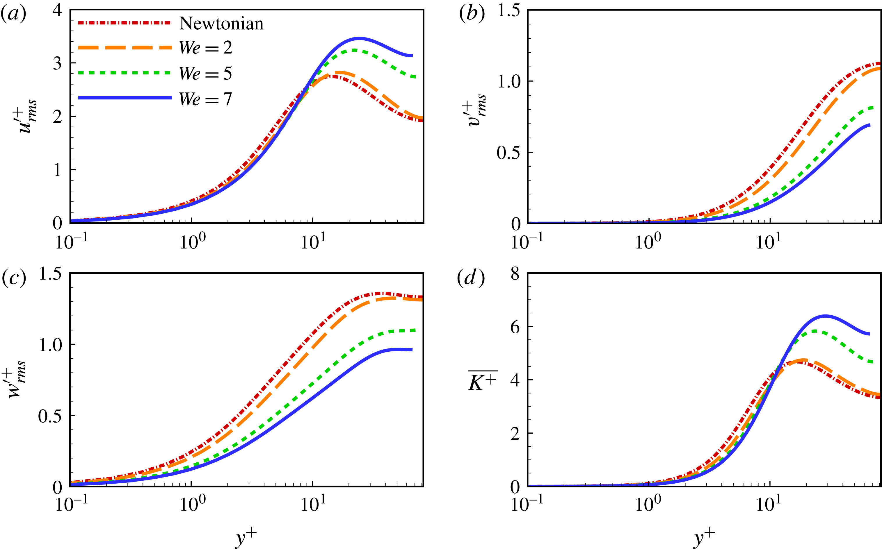
To examine the turbulent motion in drag-reduced PCF, the r.m.s. values of velocity fluctuations are shown in figure 5. For PPF of LDR, the polymeric additive is found to suppress the energy redistribution from the streamwise to the wall-normal and spanwise fluctuating motions, which leads to an increase in streamwise velocity fluctuation in the buffer and log layers and a decrease in the other two components (Min et al. Reference Min, Yoo, Choi and Joseph2003b ; Stone et al. Reference Stone, Roy, Larson, Waleffe and Graham2004; Li et al. Reference Li, Sureshkumar and Khomami2006, Reference Li, Sureshkumar and Khomami2015). In the high drag reduction (HDR) regime of PPF, all three components of r.m.s. velocities are suppressed. For drag-reduced PCF, the r.m.s. value of velocity fluctuations exhibits polymer-induced variations in a manner similar to that of PPF at LDR. Namely, introducing polymer additives serves to enhance the r.m.s. value of streamwise velocity fluctuations, i.e. the streamwise fluctuating motions, and to suppress the other two components (see figure 5 a–c). With the increase of $We$ , this effect of polymer additives becomes more pronounced. Moreover, the peak values of the turbulent kinetic energy (see figure 5 d) shift away from the wall, indicating the broadening of the buffer layer. This near-wall turbulence behaviour has also been found in drag-reduced PPF.

Figure 6.

Distribution of r.m.s. value of streamwise vorticity fluctuation.

Figure 7.

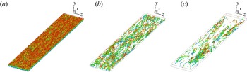
Vortical (elliptical) structures visualized by instantaneous $Q$ -criterion with $Q=0.1$ and coloured by the distance to the lower wall for Newtonian PCF (a), $We=5$ (b) and $We=7$ (c).

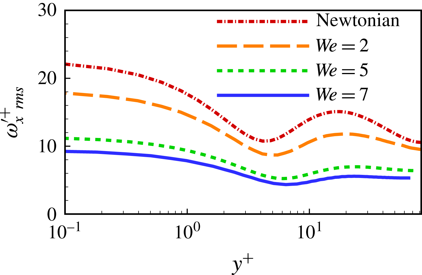
The effect of polymer elasticity on near-wall quasi-streamwise vortices (QSVs) can be examined by the r.m.s. value of streamwise vorticity fluctuation ( $\unicode[STIX]{x1D714}_{x~rms}^{\prime +}$ ) (see figure 6). According to Kim et al. (Reference Kim, Moin and Moser1987), the $y$ - positions of the local minimum and maximum of $\unicode[STIX]{x1D714}_{x~rms}^{\prime +}$ correspond to the ensemble-averaged locations of the edge and centre of the QSVs, respectively, and their distance is roughly proportional to the size of the QSVs. When $We$ is increased from 0 to 7, $\unicode[STIX]{x1D714}_{x~rms}^{\prime +}$ decreases substantially, and the difference between the local minimum and maximum of $\unicode[STIX]{x1D714}_{x~rms}^{\prime +}$ becomes more and more subtle. This points to a drag-reduction-related weakening process of QSVs. The weakening of QSVs is a common feature in drag-reduced shear flow (Stone et al. Reference Stone, Roy, Larson, Waleffe and Graham2004), that results in less energetic ejection and sweep events in the buffer layer. Moreover, the local minimum and maximum of $\unicode[STIX]{x1D714}_{x~rms}^{\prime +}$ shift away from the wall, as a result of the broadening of the buffer layer. Note that PCF and PPF share the same polymer-induced behaviours of $\unicode[STIX]{x1D714}_{x~rms}^{\prime +}$ (Min et al. Reference Min, Yoo, Choi and Joseph2003b ; Li et al. Reference Li, Sureshkumar and Khomami2006, Reference Li, Sureshkumar and Khomami2015; Dallas et al. Reference Dallas, Vassilicos and Hewitt2010). This similarity supports studies in that the near-wall coherent structures are essentially the same for the self-sustaining mechanism of wall-bounded turbulence (Hamilton et al. Reference Hamilton, Kim and Waleffe1995; Stone et al. Reference Stone, Waleffe and Graham2002). The weakening of near-wall QSVs with the increase of $We$ can also been visualized by the instantaneous $Q$ -plot for vortical (elliptical) structures of $Q=0.1$ (see figure 7). Together with the similar weakening of extensional (hyperbolic) structures (not visualized here), this feature confirms that enhanced drag reduction is commensurate with a phenomena of flow parabolization, as found by Pereira et al. (Reference Pereira, Mompean, Thais, Soares and Thompson2017b ,Reference Pereira, Mompean, Thompson and Soares c ) in their study of transient evolution of viscoelastic PCF.

In the core region, however, the behaviour of $\unicode[STIX]{x1D714}_{x~rms}^{\prime +}$ is markedly different between drag-reduced PPF and PCF. As for viscoelastic PPF at LDR, $\unicode[STIX]{x1D714}_{x~rms}^{\prime +}$ in the core region is much less than that in the near-wall region (Li et al. Reference Li, Sureshkumar and Khomami2006, Reference Li, Sureshkumar and Khomami2015; Dallas et al. Reference Dallas, Vassilicos and Hewitt2010). However, for the drag-reduced PCFs considered here, the values of $\unicode[STIX]{x1D714}_{x~rms}^{\prime +}$ in the core region and near-wall region are comparable (see figure 6). This difference is associated with the presence of roll cells that appear in the core region of PCF. Such roll cells behave like counter-rotating QSVs of a much larger scale and contribute to generate additional streamwise vorticity fluctuations in the core region. The strength of QSVs in the core region decreases with increasing $We$ (see figure 6); this is consistent with the trend observed in the simplified linear problem of roll–streak interaction in viscoelastic Couette flow (Page & Zaki Reference Page and Zaki2014).

The scale of coherent structures changing with the increasing polymer elasticity can be quantified by the two-point correlations. Specifically, an increase of spanwise scale occurs for the near-wall coherent structures. In figure 2(b), the first minimum of near-wall $R_{uu}(\unicode[STIX]{x0394}z)$ is indicative of the spanwise spacing of near-wall coherent structures. As stated above, the first minimum of $R_{uu}(\unicode[STIX]{x0394}z)$ for $y^{+}=8$ occurring at $\unicode[STIX]{x0394}z\approx 0.73$ indicates a spanwise spacing of $\unicode[STIX]{x0394}z^{+}\approx 120$ for the near-wall coherent structures. At the channel centre $(y^{+}=82)$ , $R_{uu}(\unicode[STIX]{x0394}z)$ has its first minimum occurring at $\unicode[STIX]{x0394}z\approx 1.85$ , corresponding to a spanwise scale of LSSs in the core region of $\unicode[STIX]{x0394}z\approx 3.70$ for LSSs. As $We$ is increased from 0 to 7, the near-wall coherent structures scale grows in the spanwise direction as the first minimum of $R_{uu}(\unicode[STIX]{x0394}z)$ occurs at a larger value of $\unicode[STIX]{x0394}z$ ; however, spanwise scales of the core-region LSSs remain almost unaltered. Increase in spanwise scale of near-wall coherent structures is a common feature of drag-reduced PPF (Li et al. Reference Li, Sureshkumar and Khomami2006; White & Mungal Reference White and Mungal2008). The results shown here confirm that the same is true for drag-reduced PCF.

4 Flow behaviour in the core region

As addressed above, differences between turbulent PCF and PPF exist mainly in the core region. Large-scale streaks and roll cells have been found in the core region of PCF but not in PPF. This is the main difference between PCF and PPF. Another significant difference is that a non-zero mean flow shear rate is present in PCF. To this end, in the discussion that follows, turbulence dynamics in the core region of drag-reduced PCF is scrutinized.

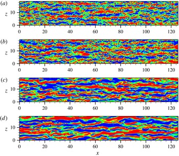
The large-scale streaks can be visualized at the channel centre by the streaky patterns of positive and negative streamwise velocity fluctuations alternating along the spanwise direction (see figure 8). As $We$ is increased from 0 to 7, the longitudinal length scales of the large-scale streaks increase, making the streaks more distinguishable. This change indicates an enhanced growth of large-scale streaks due to polymer elasticity, consistent with the findings of a recent study on instability of streak evolution (Page & Zaki Reference Page and Zaki2014). In parallel, the intensity of the streaks indicates an enhancement of streamwise fluctuating motions.

Figure 8.

Visualization of streaky structures by instantaneous streamwise velocity fluctuation in the $x{-}z$ plane at channel centre, (a) Newtonian flow, (b) $We=2$ , (c)  $We=5$ and (d) $We=7$ . Twenty contours are shown in $(-0.1,0.1)$ .

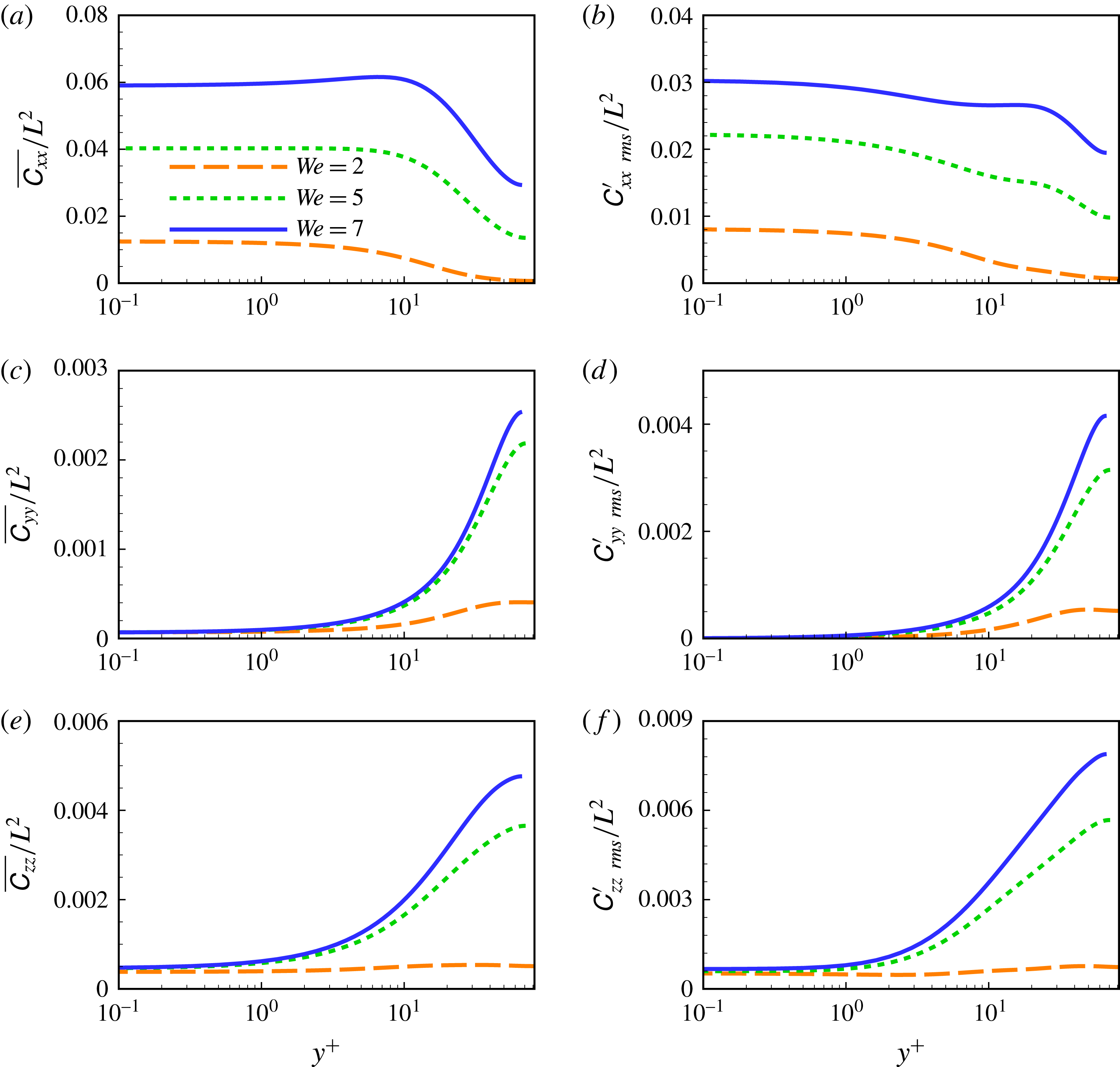
To better understand PCF polymer dynamics, mean values of the conformation tensor components and their fluctuations are examined (see figure 9). Specifically, it can be seen in figure 9(a) that the mean value of $\unicode[STIX]{x1D60A}_{xx}$ has its maximum in the wall region at low $We$ , namely, $We=2$ , and in the buffer layer at high $We$ ( $We=7$ ). This feature is basically the same as drag-reduced PPF (Dallas et al. Reference Dallas, Vassilicos and Hewitt2010). Note for drag-reduced PCF, the mean value of $\unicode[STIX]{x1D60A}_{xx}$ in the core region is approximately half of that of the near-wall region, while the mean values of $\unicode[STIX]{x1D60A}_{yy}$ and $\unicode[STIX]{x1D60A}_{zz}$ (see figures 9 c and 9 e) are approximately zero in the wall region with their maxima occurring at the channel centre. This is strikingly different from the case of drag-reduced PPF (Li et al. Reference Li, Sureshkumar and Khomami2006; Dallas et al. Reference Dallas, Vassilicos and Hewitt2010). The large mean values of $\unicode[STIX]{x1D60A}_{xx}$ , $\unicode[STIX]{x1D60A}_{yy}$ and $\unicode[STIX]{x1D60A}_{zz}$ occurring at the channel centre are ascribed to high polymer stretching related to the mean flow shear and LSSs in the core region. Basically, the fluctuations of $\unicode[STIX]{x1D60A}_{xx}$ , $\unicode[STIX]{x1D60A}_{yy}$ and $\unicode[STIX]{x1D60A}_{zz}$ have similar distributions to the main values of these components in the conformation tensor. Thus, mean polymer stretch and its fluctuating part are enhanced in turbulent PCF with the increase of $We$ .

Figure 9.

Mean and r.m.s. values of the conformation tensor component $\unicode[STIX]{x1D60A}_{xx}$ , $\unicode[STIX]{x1D60A}_{yy}$ and $\unicode[STIX]{x1D60A}_{zz}$ for different $We$ .

Figure 10.

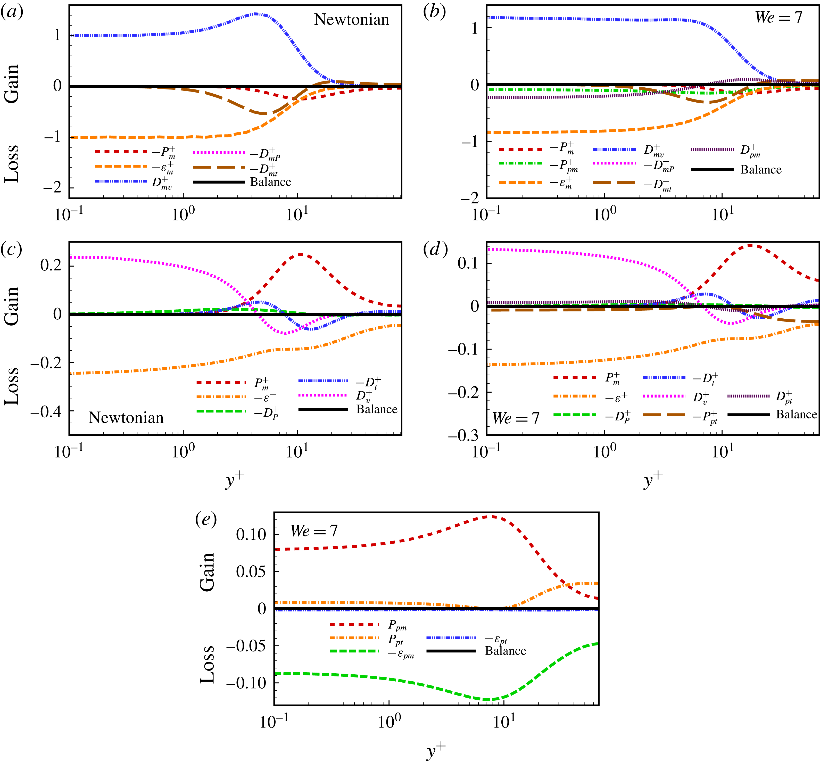
The budgets for mean kinetic energy $K_{m}^{+}$ (a,b), turbulent kinetic energy $K^{+}$ (c,d) and elastic potential energy $E_{p}^{+}$ (e).

To examine the influence of polymer stretch on energy exchange in the core region, the budgets of mean kinetic energy (MKE), turbulent kinetic energy (TKE) and elastic potential energy (EPE) are analysed. This has been shown to be a good starting point to advance mechanistic understanding of drag reduction in drag-reduced PPF (Dimitropoulos et al. Reference Dimitropoulos, Sureshkumar, Beris and Handler2001; Min et al. Reference Min, Choi and Yoo2003a ,Reference Min, Yoo, Choi and Joseph b ; Dallas et al. Reference Dallas, Vassilicos and Hewitt2010; Tsukahara et al. Reference Tsukahara, Ishigamia, Yub and Kawaguchia2011; Thais et al. Reference Thais, Gatskid and Mompeana2012, Reference Thais, Gatskid and Mompeana2013). In the following, we focus on the budget terms of key importance to the energy exchange process. Specifically, the production terms $P_{m}^{+}$ , $P_{pm}^{+}$ and $P_{pt}^{+}$ represent energy exchange from MKE to TKE, from MKE to EPE and from TKE to EPE, respectively; $\unicode[STIX]{x1D700}_{m}^{+}$ and $D_{m\unicode[STIX]{x1D708}}^{+}$ denote respectively viscous dissipation and diffusion of MKE; $D_{mP}^{+}$ and $D_{mt}^{+}$ are the mean pressure and turbulent transport terms, respectively; and $D_{pm}^{+}$ and $D_{pt}^{+}$ are the polymeric transport terms for MKE and TKE, respectively. A detailed description of the budget equations for MKE, TKE and EPE is given in appendix A.

In figure 10(a–d), the budget terms of MKE and TKE for Newtonian flow are compared with those of drag-reduced PCF at $We=7$ ; the budget terms of EPE are also plotted in figure 10(e). The balances achieved in these three budgets provide a further evidence that statistically steady states have been realized in our calculations. Here, some differences between PCF and PPF can be clearly seen. For the budget of MKE, it is shown (see figure 10 a) that viscous diffusion $D_{m\unicode[STIX]{x1D708}}^{+}$ is positive (i.e. a source term) across the channel for Newtonian PCF; however, for PPF, this term changes from positive to negative as one moves away from the wall (Thais et al. Reference Thais, Gatskid and Mompeana2013). In contrast, turbulent transport term $D_{mt}^{+}$ is positive across the channel for PPF but changes from positive to negative for PCF. Moreover, non-zero values of $P_{m}^{+}$ and $\unicode[STIX]{x1D700}_{m}^{+}$ can be observed in the core region of PCF; however, for PPF, all the budget terms of MKE approach zero in this region. This is the most distinct difference between PCF and PPF, and it originates from the non-zero mean flow shear in the core region, as discussed above.

With respect to the MKE budget of drag-reduced PCF (see figure 10 b), two extra terms are added, namely, the polymer transport term $D_{pm}^{+}$ and energy production term $P_{pm}^{+}$ . $-P_{pm}^{+}$ is negative across the channel, which means that the polymer chains absorb energy from the MKE in the entire domain. In the core region, $-P_{pm}^{+}$ is comparable to other budget terms. In contrast, drag-reduced PPF has a negligibly small value of $P_{pm}^{+}$ in the core region (Thais et al. Reference Thais, Gatskid and Mompeana2013). This comparison also highlights the difference of flows in the core region between viscoelastic PCF and PPF. Note in figure 10(b) that the polymer transport term $D_{pm}^{+}$ changes its sign from negative to positive when one moves away from the wall; the opposite is true in the case of PPF.

For Newtonian PCF, the budget of TKE of is very similar to that of PPF (Thais et al. Reference Thais, Gatskid and Mompeana2013), except in the core region where TKE has production and dissipation terms that are very large for PCF although negligibly small for PPF (see figure 10 c). For viscoelastic PCF, two polymer-related terms, the energy exchange term, $P_{pt}^{+}$ and the polymeric transport term, $D_{pt}^{+}$ , are added. The $P_{pt}^{+}$ term has been regarded to quantify energy exchange between TKE and EPE. Specifically, negative $-P_{pt}^{+}$ means that the kinetic energy carried by fluctuating motions is absorbed and stored as elastic potential energy of stretched polymer chains; positive $-P_{pt}^{+}$ means that elastic potential energy is released from the stretched polymer chains to turbulent motions. Thus, the $P_{pt}^{+}$ term is of great importance in evaluating the interaction between turbulent motions and polymer stretching (Min et al. Reference Min, Choi and Yoo2003a ,Reference Min, Yoo, Choi and Joseph b ; Dallas et al. Reference Dallas, Vassilicos and Hewitt2010; Tsukahara et al. Reference Tsukahara, Ishigamia, Yub and Kawaguchia2011). According to Tsukahara et al. (Reference Tsukahara, Ishigamia, Yub and Kawaguchia2011), the flow domain of drag-reduced PPF can be divided along the vertical direction into three regions based on the sign of $P_{pt}^{+}$ , namely, the wall vicinity region with $-P_{pt}^{+}<0$ , the near-wall region with $-P_{pt}^{+}>0$ and the core region with $-P_{pt}^{+}<0$ . Therefore, the polymer chains absorb energy from turbulence fluctuations in the near-wall region, and begin to release their stored energy back to turbulence when they migrate away from the wall before approaching the core region.

Figure 11.

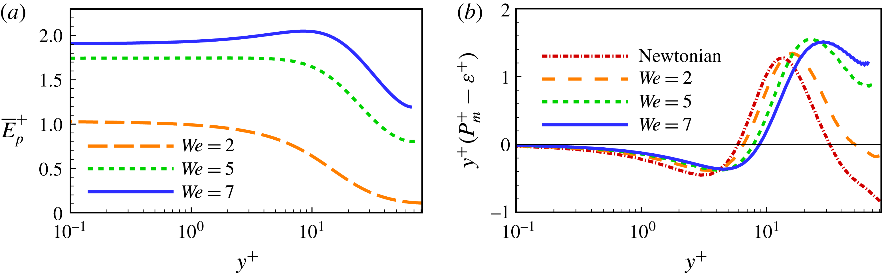
The mean elastic potential energy (a) and pre-multiplied energy production excess (b).

For drag-reduced PCF, three similar regions are also seen in figure 10(d), although the second region is not clearly distinguishable due to its very narrow interval and small magnitude. However, in the core region $-P_{pt}^{+}$ has a negative increase toward the channel centre, while for PPF it decreases in magnitude to zero. In figure 10(d), the minimum of $-P_{pt}^{+}$ occurring at the channel centre indicates that the polymer chains have the largest rate of energy absorption from turbulence in the core region. This intriguing phenomenon accounts for the considerable polymer stretch in the core region of PCF, as indicated in figure 9. At the same time, the production term $P_{m}^{+}$ becomes larger in the core region to maintain the budget balance, which in turn leads to a larger production/dissipation ratio. According to Lam & Banerjee (Reference Lam and Banerjee1992), the production/dissipation ratio is indicative of the formation of streaks: the larger the ratio, the more intensive the streaks. Therefore, in the core region of PCF, production/dissipation ratio is enhanced as a consequence of significant energy absorbed from turbulence fluctuations. This provides a plausible explanation as to why the large-scale longitude streaks strengthen, as depicted in figure 8.

Figure 10(e) illustrates the EPE budget of $We=7$ . It is seen by $P_{pm}^{+}$ and $P_{pt}^{+}$ that the polymers practically absorb energy from the MKE and TKE in the entire channel; this energy is then dissipated by the relaxation of polymer chains from an extended to an equilibrium state. Unlike drag-reduced PPF where the largest polymer dissipation occurs at the wall (Ptasinski et al. Reference Ptasinski, Boersma, Nieuwstadt, Hulsen, van den Brule and Hunt2003), the largest polymer dissipation in PCF occurs in the buffer layer. More distinct differences occur in the core region. Specifically, for drag-reduced PPF (Thais et al. Reference Thais, Gatskid and Mompeana2013), all the EPE budget terms are trivially small in the core region; however, for drag-reduced PCF, they are large. This indicates substantial energy absorption by polymers from the MKE and TKE, which is balanced by dissipation via polymer relaxation. This polymeric behaviour can be confirmed by the distribution of the mean elastic potential energy (MEPE; see figure 11 a), where the MEPE has a value in the core region of two thirds of its wall value. In contrast, for PPF, the MEPE vanishes near the centre (Thais et al. Reference Thais, Gatskid and Mompeana2013). Note that polymer chains absorb energy mainly from the MKE in the near-wall region, but from the TKE in the core region.

The energy production excess, defined as the TKE production $P_{m}^{+}$ over the dissipation $\unicode[STIX]{x1D700}$ , is plotted in pre-multiplied form in figure 11(b), so that equal areas underneath the curves correspond to equal integral contributions (Pirozzoli et al. Reference Pirozzoli, Bernardini and Orlandi2014). The energy production excess has a Newtonian peak value at $y^{+}\sim 10$ where the near-wall turbulence self-sustaining cycle is most energetic. It shifts away from the wall with the increase of $We$ as a consequence of thickening of the buffer layer. Here, the most intriguing change of the energy production excess occurs in the core region. Specifically, a significant increase from a Newtonian negative value to a much higher positive value at $We=7$ is observed. Together with the prominent energy absorption by polymer chains, this results in the great increase of TKE in the core region (see figure 5 d).

5 Effects of large-scale structures

It has been found that LSSs have a great influence on Newtonian turbulent PCF (Komminaho et al. Reference Komminaho, Lundbladh and Johansson1996; Tsukahara et al. Reference Tsukahara, Kawamura and Shingai2006). However, their influence on drag-reduced viscoelastic flow is unknown. In what follows, our initial exploration into the effects of LSSs in drag-reduced PCF is discussed.

Figure 12.

Pre-multiplied spanwise spectral density $k_{z}E(k_{z})$ ( $\int _{0}^{\infty }E_{u_{i}u_{i}}(k_{z})\,\text{d}k_{z}=\overline{u_{i}^{\prime 2}}$ ) normalized by $\overline{u_{i}^{\prime 2}}$ and varying with wall distance for Newtonian flow (a,d,g), $We=5$ (b,e,h) and $We=7$ (c,f,i). (a–c) $k_{z}E_{uu}$ ; (d–f) $k_{z}E_{vv}$ ; (g–i) $k_{z}E_{ww}$ . Twenty contour levels are shown, from 0.16 to 0.4.

Figure 13.

Pre-multiplied spanwise spectral density of velocity fluctuations at different wall distances for Newtonian flow (a,d,g), $We=5$ (b,e,h) and $We=7$ (c,f,i). (a–c) $K_{z}E_{uu}$ ; (a–c) $K_{z}E_{vv}$ ; (a–c) $K_{z}E_{ww}$ .

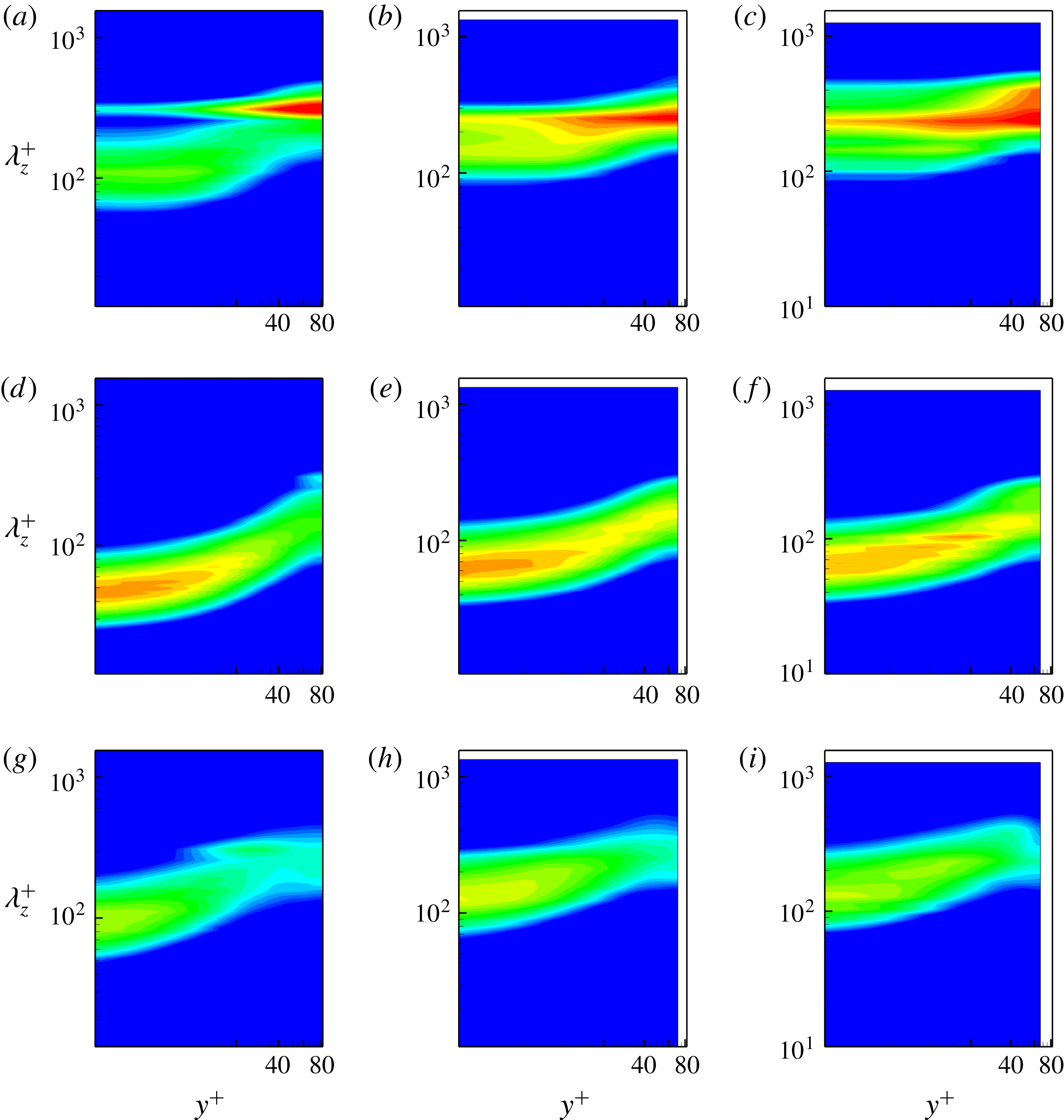
The imprint effects of LSSs on near-wall turbulence are clearly evidenced by the pre-multiplied energy spectra (see figure 12; the spectral density of $We=2$ is not shown for the sake of brevity; it has no significant difference as compared to the Newtonian case), as well as the change in length scales of coherent structures in the near-wall region and LSSs in the core region (Kim & Adrian Reference Kim and Adrian1999; Guala et al. Reference Guala, Hommema and Adrian2006; Tsukahara et al. Reference Tsukahara, Kawamura and Shingai2006; Monty et al. Reference Monty, Hutchins, Ng, Marusic and Chong2009; Pirozzoli et al. Reference Pirozzoli, Bernardini and Orlandi2014). For Newtonian PCF (see figure 12 a), two energy-condensed zones can be seen in the near-wall region but only one can be seen in the core region. The energy-condensed zone centred at $\unicode[STIX]{x1D706}_{z}^{+}\sim 100$ represents the typical self-sustained coherent structures of spanwise wavelength of approximately 100 wall units in the buffer layer. This is similar to other canonical wall-bounded shear turbulence in the near-wall region (Monty et al. Reference Monty, Hutchins, Ng, Marusic and Chong2009). Even though $Re$ in our calculation is relatively low compared to the recent study of Pirozzoli et al. (Reference Pirozzoli, Bernardini and Orlandi2014), the energy-condensed zone in the core region is still distinct due to the presence of LSSs. The imprint effect of LSSs is clearly evidenced by the secondary near-wall energy-condensed zone centred at about $\unicode[STIX]{x1D706}_{z}^{+}=300$ . This indicates that the LSSs have an average spanwise wavelength of approximately 300 wall units, corresponding to a wavenumber of ${\sim}5/3$ in the spanwise direction. For other canonical wall-bounded turbulence such as PPF and turbulent boundary layer, this secondary near-wall energy-condensed zone appears only at a much higher $Re$ . The imprint effects of LSSs help to explain why the spanwise scale of near-wall flows estimated by two-point correlations (see figure 2 a) is approximately 120 as opposed to 100 in wall units. Specifically, the estimate based on two-point correlations yields a spanwise scale larger than that of near-wall small-scale coherent structures but smaller than that of LSSs.

The introduction of polymer additives into Newtonian PCF has a great influence on both coherent structures in the near-wall region and LSSs in the core region. As depicted in figures 12(b) and 12(c), the first energy-condensed zone corresponds to coherent structures centred at larger $\unicode[STIX]{x1D706}_{z}^{+}$ , i.e. $\unicode[STIX]{x1D706}_{z}^{+}=148$ for $We=5$ and $\unicode[STIX]{x1D706}_{z}^{+}=158$ for $We=7$ . This change indicates that the increase in the spanwise scale of self-sustained coherent structures in the buffer layer is due to the polymer addition. It has been noted that a formula proposed by (Tiederman Reference Tiederman1990) and verified by Sureshkumar et al. (Reference Sureshkumar, Beris and Handler1997) can be used to link the streak spacing with the extent of drag reduction as $\unicode[STIX]{x1D706}_{z}^{+}=1.9DR\,\%+99.7$ . Accordingly, drag reduction of $26\,\%$ for $We=5$ and $34\,\%$ for $We=7$ , correspond to streak spacing of 149 and 164, respectively. These $\unicode[STIX]{x1D706}_{z}^{+}$ values predicted by this formula are consistent with our simulation results. Moreover, this energy-condensed zone becomes wider in the wall-normal direction, indicating that the influence of the coherent structures in the buffer layer is enhanced by polymer addition and affects larger distances from the wall.

The change of the LSSs in the core region in response to the introduction of polymer additives is discussed below. Figure 12(b) shows that for $We=5$ , the energy-condensed zone in the core region is centred at $\unicode[STIX]{x1D706}_{z}^{+}\sim 260$ ; still corresponding to the wavenumber ${\sim}5/3$ for LSSs in the spanwise direction. Thus, the spanwise scale of the LSSs stays unchanged. Moreover, the secondary near-wall energy-condensed zone has an enhanced contribution, which reflects that the LSSs have stronger imprint effects on the near-wall turbulence. When $We$ increases further to 7, the core-region energy-condensed zone indicates that the LSSs have the same wavenumber, i.e. ${\sim}5/3$ in the spanwise direction, while the imprint effects become more significant and penetrate the whole channel. Overall, figure 12(a–c) shows that the energy spectra in the near-wall region are dominated by coherent structures for Newtonian PCF, and the LSSs’ contribution increases monotonically with increasing $We$ for drag-reduced cases. However, at $We$ of 7, the energy spectra of near-wall turbulence is dominated by imprint effects of LSSs.

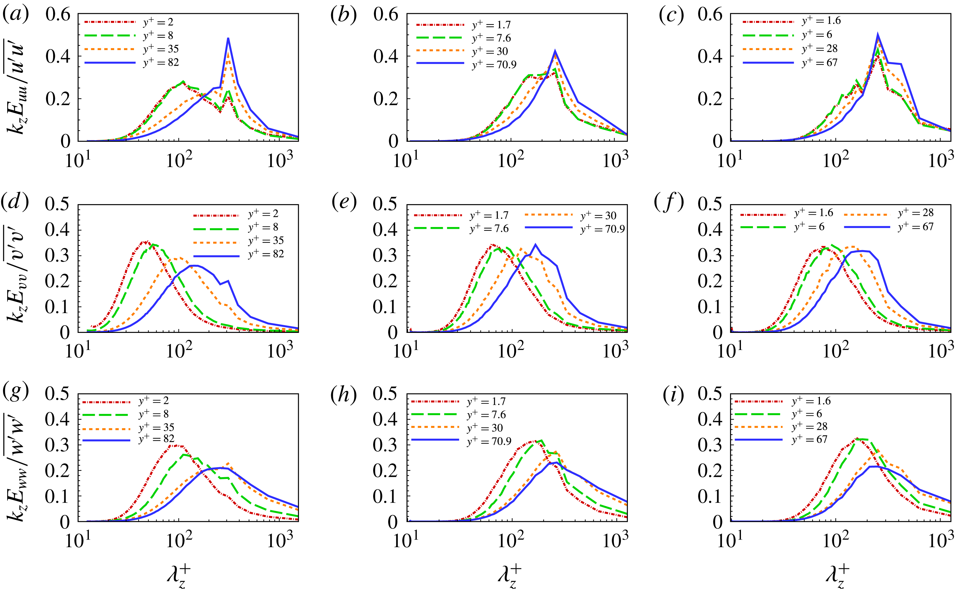
Figure 13 presents the pre-multiplied energy spectra at different wall distances. In the near-wall region, two distinct peaks can be identified for the spectra of the streamwise velocity fluctuation. The first peak denotes the spanwise scale of self-sustained coherent structures; the second one corresponds to the imprint effects of LSSs. In the core region, only one peak occurs, which denotes the spanwise scale of LSSs. With the increase of $We$ , the first near-wall peak of the spectra occurs at $\unicode[STIX]{x1D706}_{z}^{+}\sim 100$ for Newtonian PCF and it changes to $\unicode[STIX]{x1D706}_{z}^{+}\sim 148$ for $We=5$ and $\unicode[STIX]{x1D706}_{z}^{+}\sim 158$ for $We=7$ . This quantitatively demonstrates that the coherent structures have a substantial increase in spanwise scale in the near-wall region. However, the second near-wall peak and the core-region peak of the spectra both correspond to the fact that the wavenumber in the spanwise direction is ${\sim}5/3$ , which remains unaltered with the increase of $We$ . This is consistent with the estimate based on figure 12.

Figure 14.

Cumulative fraction of the streamwise kinetic energy $\unicode[STIX]{x1D6FE}_{uu}$ (a) and of the Reynolds stress $\unicode[STIX]{x1D6FE}_{uv}$ (b) at $y^{\ast }=0.1$ where $y^{\ast }$ is the wall distance. The symbols in the plots represent the spanwise scales of LSSs for different calculations.

The influence of LSSs can be quantified by examining the relative contributions of different wavelengths to the total energy (or shear stress). The cumulative contributions to $\overline{u_{i}^{\prime }u_{j}^{\prime }}$ are evaluated in spectral space as

(5.1) $$\begin{eqnarray}\displaystyle & \unicode[STIX]{x1D6FE}_{ij}(k_{z})=1-{\displaystyle \frac{\displaystyle \mathop{\sum }_{0}^{k}E_{ij}(\tilde{k_{z}})}{\displaystyle \mathop{\sum }_{0}^{k_{max}}E_{ij}(\tilde{k_{z}})}}, & \displaystyle\end{eqnarray}$$

where $E_{ij}$ is the spectral density of $\overline{u_{i}^{\prime }u_{j}^{\prime }}$ (Guala et al. Reference Guala, Hommema and Adrian2006; Balakumar & Adrian Reference Balakumar and Adrian2007). $\unicode[STIX]{x1D6FE}_{ij}(k_{z})$ denotes the relative contribution of large-scale motions with wavenumber ${>}k_{z}$ . 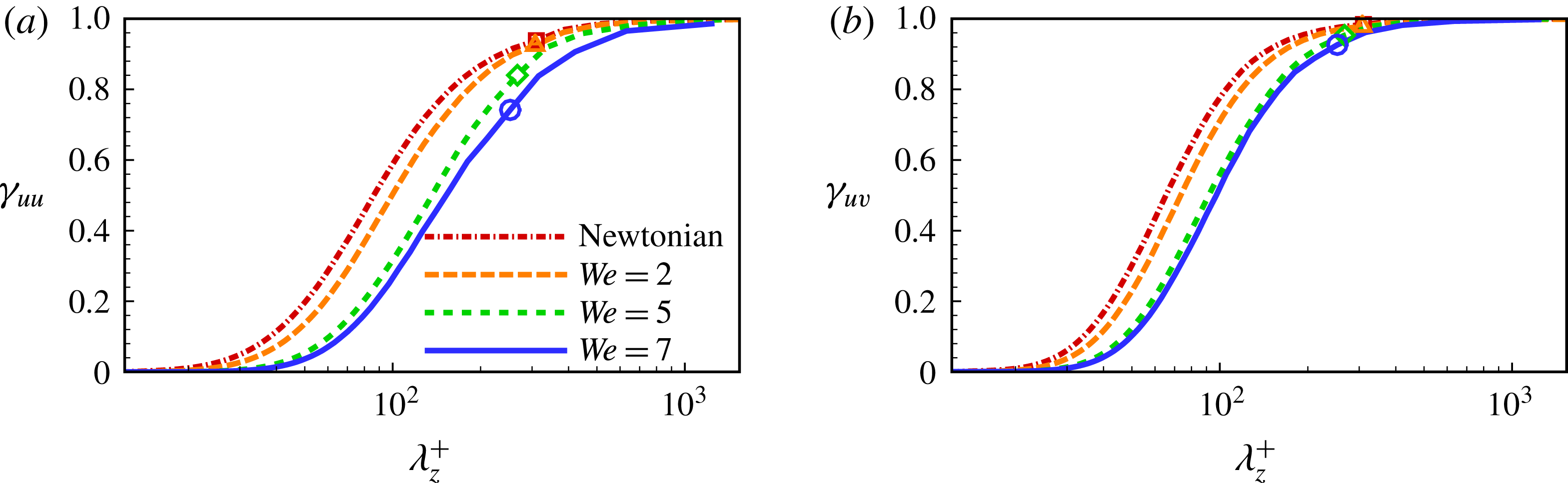The cumulative contributions $\unicode[STIX]{x1D6FE}_{uu}(k_{z})$ and $\unicode[STIX]{x1D6FE}_{uv}(k_{z})$ have been calculated in the near-wall region (see figure 14). It is indicated that the relative contribution of large-scale motions substantially increases with the increase of $We$ . Note that the spanwise scales of LSSs are denoted by symbols in the plots. From $\unicode[STIX]{x1D6FE}_{uu}(k_{z})$ , the large scales ( ${\geqslant}$ the spanwise scales of LSSs) have a cumulative contribution of $6\,\%$ for Newtonian PCF, which increases to $8\,\%$ for $We=2$ , then to $16\,\%$ for $We=5$ and eventually to $26\,\%$ for $We=7$ . As for $\unicode[STIX]{x1D6FE}_{uv}(k_{z})$ , a corresponding increase in cumulative contribution is found from $1.6\,\%$ to $2.1\,\%$ , then to $5\,\%$ , and eventually to $7\,\%$ . These two changes likely stem from the increasing imprint effects of LSSs on the near-wall flow.

The nonlinear effects of LSSs on the near-wall flows can be quantified by an amplitude modulation coefficient calculated using the Hilbert transform and a Fourier filter (Mathis et al. Reference Mathis, Hutchins and Marusic2009). The modulation coefficient has a strong resemblance to the skewness profile of $u^{\prime }$ (Mathis et al. Reference Mathis, Marusic, Hutchins and Sreenivasan2011). 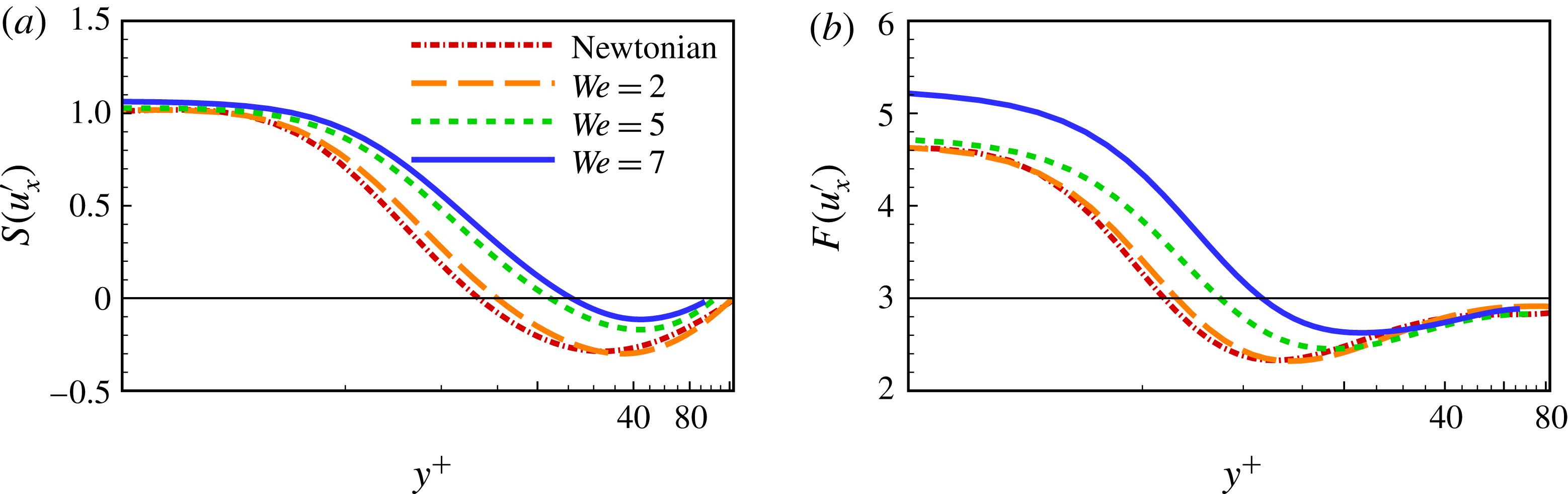To this end, the skewness of $u^{\prime }$ is examined here to ascertain the effects of modulation on the LSSs. As shown in figure 15(a), the skewness increases monotonically with the increase of $We$ , indicating an enhancement of the modulation effects of LSSs. Moreover, the increase of the skewness implies that the asymmetry of the streamwise fluctuations is enhanced. Also, the flatness increases monotonically with the increase of $We$ (see figure 15 b), which suggests a stronger intermittency of streamwise fluctuating motions (Pirozzoli et al. Reference Pirozzoli, Bernardini and Orlandi2014). The increased near-wall intermittency has also been related to the modulation imparted by LSSs (Mathis et al. Reference Mathis, Hutchins and Marusic2009) and is consistent with the explanation that drag reduction is commensurate with an increased interval of hibernating turbulence (Xi & Graham Reference Xi and Graham2012). With the increase of $We$ , the skewness and flatness of $u^{\prime }$ in the near-wall region demonstrate a clear deviation from the Gaussian behaviour, namely, $S(u^{\prime })=0$ and $F(u^{\prime })=3$ , while at the channel centre they are close to the Gaussian values. This is very different from the findings of Samanta et al. (Reference Samanta, Housiadas, Handler and Beris2009) in drag-reduced PPF especially in the core region.

Figure 15.

The skewness (a) and flatness (b) of the streamwise velocity fluctuation, defined as $S(u^{\prime })\equiv \overline{{u^{\prime }}^{3}}/(\overline{u^{\prime 2}})^{3/2}$ and $F(u^{\prime })\equiv \overline{{u^{\prime }}^{4}}/(\overline{u^{\prime 2}})^{2}$ , respectively.

The increasing effects of LSSs on the near-wall flow are further evidenced by the monotonic increase of the peak value of $u_{rms}^{\prime +}$ shown in figure 5(a). According to previous studies (Marusic et al. Reference Marusic, Mathis and Hutchins2010; Orlandi et al. Reference Orlandi, Bernardini and Pirozzoli2015; Smits Reference Smits2015), for Newtonian turbulence, the peak value of $u_{rms}^{\prime +}$ should be invariant to the increase of $Re$ if not affected by fluid flow above the buffer layer; however, the effects of core-region LSSs do indeed cause a deviation. Thus, the enhancement of $u_{rms}^{\prime +}$ peak value due to the increase of $We$ (see figure 5 a) results from the increasing influence of the LSSs on near-wall turbulence. This is consistent with the above discussions which indicate that the imprint and modulation effects of LSSs are enhanced in drag-reduced PCF.

Figure 16.

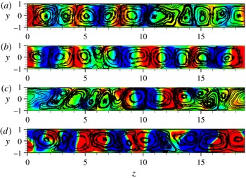
Large-scale structures (roll cells) visualized by streamline plots of the ensemble-averaged velocity vector $(\boldsymbol{v},\boldsymbol{w})$ for Newtonian flow (a) and drag-reduced flows with $We=2$ (b), $We=5$ (c) and $We=7$ (d) (Komminaho et al. Reference Komminaho, Lundbladh and Johansson1996; Avsarkisov et al. Reference Avsarkisov, Hoyas, Oberlack and García-Galache2014). The ensemble average is performed in time and streamwise directions. The contour denotes the value of streamwise velocity fluctuation. Twenty contours are plotted in $(-0.02,0.02)$ . Five pairs of roll cells can be seen in all the figures.

The roll cells appearing in PCF are reminiscent of the well-known Taylor vortices found in Taylor–Couette flow. However, the Taylor vortices and the roll cells discussed here are distinct, because the Taylor vortices are formed as a consequence of a centrifugal instability while the roll cells are formed due to a quasi-periodic process in which low-speed velocity streaks generate large-scale vortices (Hamilton et al. Reference Hamilton, Kim and Waleffe1995). The roll cells can be visualized by streamline plots based on the velocity vector $(\boldsymbol{v},\boldsymbol{w})$ averaged in time and in the streamwise direction (Komminaho et al. Reference Komminaho, Lundbladh and Johansson1996; Avsarkisov et al. Reference Avsarkisov, Hoyas, Oberlack and García-Galache2014; Niebling et al. Reference Niebling, Tallakstad, Toussaint and Måløy2014). In figure 16, the roll cells, composed of 5 pairs of counter-rotating vortices, are clearly visualized for Newtonian PCF and drag-reduced flows. Note that this number of roll cell pairs corresponds to a wavenumber of ${\sim}5/3$ in the spanwise direction. These well-shaped structures can be obtained only by ensemble averaging based on a sufficiently large sample size of flow fields, especially at high $Re$ . As shown in figure 16, the roll cells penetrate the entire channel and thus have a vertical scale of the channel height. Evidently, these roll cells should be treated as LSSs.

Next, we would like to recall some evidence that implies that the roll cells are the key LSSs in the core region. First, as predicted by $R_{uu}(\unicode[STIX]{x0394}z)$ in figure 2(b,d,f), the LSSs in the core region have a spanwise scale of approximately 3.70, corresponding to the number of roll cell pairs of $N=6\unicode[STIX]{x03C0}/3.70\approx 5$ . This prediction agrees well with the number of roll cells observed in figure 16. These roll cell structures should be responsible for the minima of $R_{uu}(\unicode[STIX]{x0394}z)$ in the core region as observed in figure 2(b,d,f) (Avsarkisov et al. Reference Avsarkisov, Hoyas, Oberlack and García-Galache2014). Second, in figures 12 and 13, the pre-multiplied spectra of the streamwise velocity fluctuation point to an estimate that the LSSs in the core region have a wavenumber of ${\sim}5/3$ in the spanwise direction. This estimate is also consistent with the number of roll cell pairs identified in figure 16. Moreover, it is shown in figure 16 that the number of roll cells stays basically the same for Newtonian and viscoelastic PCF. This feature is in good agreement with the above findings that the spanwise wavelength of LSSs remains unaltered for all the cases considered. Here, it is of special interest that the introduction of polymer additives has no influence on the spanwise scales of LSSs, namely, roll cells.