

I. Equality and Liberty
Equality of opportunity is difficult to behold, nearly impossible to measure, and likely impossible to achieve in the strictest sense of the term. Economic freedom is the nearest practical approximation of equality of opportunity, if only for the reason that it is impossible to ensure that each person is born into the exact same set of circumstances and subject to the exact same events. In short, economic freedom is the closest humans can come to equality of opportunity without suspending the laws of random chance. Like equality of opportunity, economic freedom cannot be measured directly, but its manifestations are more easily enumerated and measured: less government spending, less regulation, fewer labor restrictions, less public corruption, more protections for private property.
Economic freedom, like the more abstract notion of equality of opportunity,Footnote 1 necessarily implies inequality of outcome. Simply put, some are more skilled, gifted, and industrious than others. Against a backdrop of economic freedom, these people will succeed to a higher degree than their less skilled, less gifted, and less industrious counterparts. Luck, too, plays a significant role.
Those who advocate for equality of outcome tend to argue against economic freedom. But the fact that more economic freedom causes more unequal outcomes does not imply that less economic freedom causes less unequal, or even preferable outcomes. It is possible that the tools and methods we use to restrict economic freedom may themselves promote unequal outcomes. Those interested in achieving equality of outcome cannot know, a priori, that less economic freedom will achieve their goal, or at what cost. Instead, they must address two empirical questions:
• Does suppressing economic freedom cause more or less inequality of outcome than does securing economic freedom?
• Does suppressing economic freedom cause a greater or lesser level of outcome than does securing economic freedom?
If suppressing economic freedom causes both less outcome inequality and a greater outcome level than does securing economic freedom, then we have a solid argument in favor of a more expansive view of the proper role of government in society. Alternatively, if securing economic freedom causes both less outcome inequality and a greater outcome level, then we have a solid argument in favor of a more restrictive view of the proper role of government. But if securing economic freedom causes more (less) outcome inequality but a greater (lesser) outcome level, then we have an argument for limited economic freedom wherein we must trade some worsening (improvement) in outcome inequality for an improvement (worsening) in the outcome level.
These are causal empirical questions that can only be answered through experimentation. Absent experimental data, the best we can do is to look for correlations between economic freedom and desirable socioeconomic outcomes. While correlation does not imply causation, the absence of correlation does imply the absence of causation. So let us ask the question in the negative: Is economic freedom correlated with more outcome inequality and lesser outcome levels? If we do not find a correlation, then we know that there is also no causation. While that alone would not recommend economic freedom, it would demonstrate that securing economic freedom does not result in worse outcomes than would the suppression of economic freedom. We could then fall back on the fact that equality of opportunity requires economic freedom, and say that our quest for equality must end at achieving equality of opportunity, knowing that we have not made outcome inequality any worse than it would have been had we suppressed economic freedom.
II. Economic Freedom
The preservation of property very clearly presupposes the accumulation of property, and the accumulation of property, in turn, requires some degree of economic freedom. And while there is no purely objective way to measure economic freedom, there are metrics that make it possible to ascertain whether economic freedom yields beneficial results. In short, it is possible by measuring observable data to determine whether the liberty that many Americans consider their birthright is also a positive instrumentality in their lives individually, and more importantly, collectively.
The Fraser Institute’s Economic Freedom of North America Index (EFNA) makes a consideration of this type possible. For each of the fifty states in each year from 1981 through 2009, Fraser considers a fixed set of economic variables that are correlated with economic freedom. Fraser combines these economic variables into a single index that represents Fraser’s estimate of economic freedom in each state for each year. The index number ranges from 1 (minimal economic freedom) to 10 (maximum economic freedom). Fraser designs the index number to be absolute so that, for example, 10 represents not the maximum observed freedom but the maximum attainable freedom. Designing the index to be absolute makes it possible not only to compare economic freedoms among states in a given year, but to observe changing economic freedoms over time.
The twenty-eight economic variables Fraser uses in constructing its index fall into three groups: measures of government spending, measures of taxation, and measures of labor market freedom.Footnote 2 By way of example, some specific economic variables include: government spending within a state relative to the size of the state’s economy, government subsidies given to people and companies within a state relative to the size of that state’s economy, total tax revenue relative to the size of that state’s economy, top marginal income tax rates and the thresholds at which they apply, government employment relative to total employment within that state, and minimum wage legislation.Footnote 3
There is no purely objective way to measure economic freedom, but the EFNA is a quasi-objective measure in that, while the researchers choose which economic variables to include in the index and how to weight them, the values of the economic variables themselves are objectively measured. For each year and each state, Fraser includes the same economic variables and applies the same weights. This means that Fraser’s definition of economic freedom remains constant across states and across years. Because the measure is quasi-objective, other economic freedom indices (for example, Mercatus Center’s Freedom in the 50 States study, and Heritage Foundation’s Index of Economic Freedom) will differ from the EFNA (and from each other), though they are all correlated. The EFNA, though, provides the longest history of freedom measures for the individual states.Footnote 4
If economic freedom is beneficial to society, this story should emerge in the data. If economic freedom is detrimental to society in specific ways, this too should be evident. The question now is what outcomes are beneficial to society? We look at five categories of outcomes that are important to human flourishing: incomes (as measured by median household income and per-capita personal income), poverty and inequality (as measured by the unemployment rate, the poverty rate, income inequality, and the percentage of uninsured people), population growth (as measured by population growth and by in-migration relative to out-migration), fiscal health of government (as measured by tax revenue and the magnitude of government debt relative to the size of the economy), and economic growth (as measured by the growth in the number of firms and growth in state GDPs). If economic freedom is beneficial, we should observe, quite simply, improved socioeconomic outcomes where we see increased economic freedom. If economic freedom is detrimental, we should observe diminished socioeconomic outcomes.Footnote 5
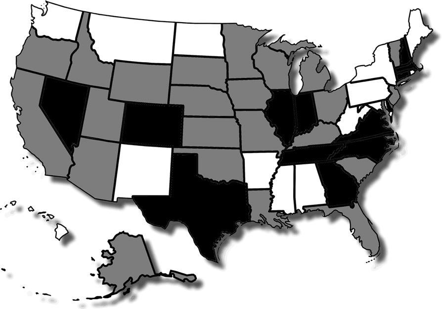
The most straightforward way to examine socioeconomic outcomes relative to economic freedom is, for each year, to divide the states into two groups: the twenty-five with economic freedom indices that are above the median economic freedom for the year (the “more free states”) and the twenty-five with indices that fall below the median for the year (the “less free states”). If economic freedom is beneficial, then the socioeconomic outcomes for the twenty-five more-free states should be significantly and obviously better than those of the socioeconomic outcomes for the twenty-five less free states. But the sets of “more free” and “less free” states are not constant over time. From 1985 to 2009, thirteen states were in the “less free” category every year, fourteen states were in the “more free” category every year, and twenty-three states switched from one category to the other at least once. Of the states that switched, the average state switched categories three times from 1985 through 2009. States that switched categories the most include California and Kansas (eight times each), Kentucky (five times), and Florida, Idaho, Ohio, Vermont, and Wisconsin (four times each). Only two states, South Dakota and Utah, switched only once. The states are shown, by category, in Figure 1.Footnote 6 The individual EFNA indices range from a low of 4.95 for West Virginia in 1986 to a high of 8.48 for Delaware in 2004. The differences in the average EFNA indices between the categories are statistically significant over all the years, both in the aggregate and in each individual year.Footnote 7
States categorized by economic freedom over time.Footnote 8

III. Incomes
A. Median household incomeFootnote 9
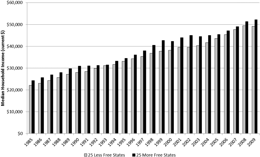
There are a variety of income measures, each of which touches on a different nuance. The measure that comports most closely with what a noneconomist would consider “income” is median household income. Average measures such as per-capita income, and average personal income can be influenced by outliers. For example, one very rich person can drive up an average income measure. Median measures are immune to outliers, as they reflect the “middle” income of the group. The measure is simply an identification of the absolute middle of the pack. Figure 2 shows median household income for the fifty states over time.
Average median household income for the least and more free states as measured by the EFNA index.Footnote 10
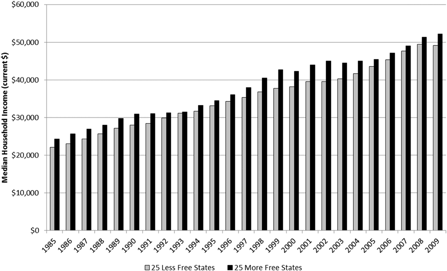
From 1985 through 2009, the average of the median household incomes for the more free states was 7.8 percent greater than the average of the median household incomes for the less free states. In each individual year, median household income was higher among the more free states and the difference ranged from a high of 13 percent more in 1999 and 2002 to a low of 1.2 percent more in 1993.Footnote 11 Not only do households in the more free states have higher median incomes than do households in the less free states on average, but the difference holds in each individual year.
A reasonable counterargument is that something other than economic freedom is driving the results. Perhaps the more free states are located in higher cost areas, or the more free states also have more large cities. This is a reasonable counterargument, though it becomes less tenable when we remember that the two groups (more free states and less free states) are not static. Almost 50 percent of the states switch groups over the years.
B. Per-capita personal incomeFootnote 12
Comparing household incomes can distort the view of earnings if there is a systemic difference in the number of income earners residing in the same household across the two samples and even across years. For example, if each worker in both sets of states earned $45,000, but the households in the more free states were all two-income households whereas the households in the less free states were all single-income households, then we would expect the median household income for the more free states to be $90,000 versus $45,000 for the less free states. Differences in household incomes can be due not only to differences in worker incomes but also to differences in the number of wage earners in the households. Per-capita personal income gets around this problem by scaling total income by the population rather than by the number of households.
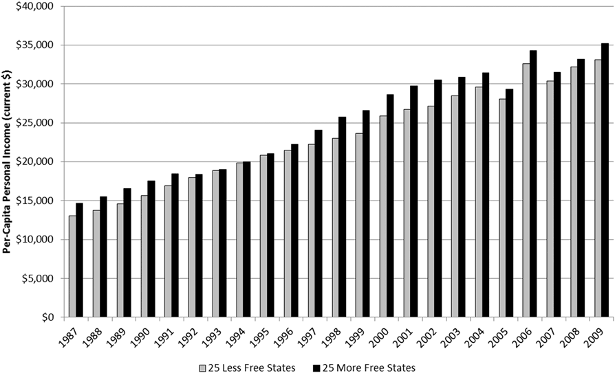
Over the sample, the average of the per-capita personal incomes for the more free states was 7.5 percent greater than the average of the per-capita personal incomes for the less free states (Figure 3). As with household income, in each individual year, per-capita personal income was higher among the more free states. The difference ranged from a high of above 13 percent in 1989 to a low of 0.8 percent in 1994 and 0.9 percent in 1995.Footnote 14 These results suggest that the systematic difference in household incomes we observed was not due to systematic differences in the number of wage earners per household.
Average per-capita personal income for the least and more free states as measured by the EFNA index.Footnote 13
IV. Poverty and Inequality
A. Unemployment rateFootnote 15
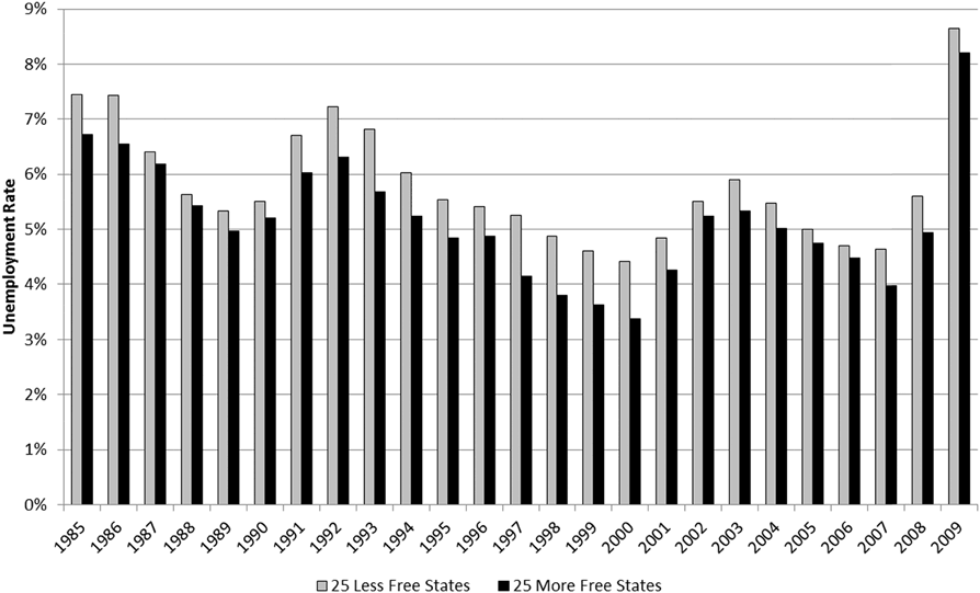
A criticism of per-capita income data is that higher incomes can mask the effects of unemployment. For example, a state in which 50 percent of the workers earn $100,000 and 50 percent are unemployed can show the same per-capita income ($50,000) as a state in which all of the workers are employed and each earns $50,000. Here too the data are revealing. From 1985 through 2009, the average unemployment rate among the more free states was lower than that of the less free states in every year (Figure 4). Throughout the period, the average unemployment rate among the more free states was 5.2 percent versus 5.8 percent among the less free states.Footnote 16
Average unemployment rates for the least and more free states as measured by the EFNA index.Footnote 17
The difference in the average unemployment rates varied from a low of 0.2 percentage points in 1987 and 1988 to a high of 1 percentage point or more in 1993 and again from 1997 through 2000. Over the sample period, the U.S. labor force averaged over 136 million workers. Assuming the labor force is evenly distributed among the most and less free states, the lower unemployment rate among the more free states was equivalent to 860,000 jobs.Footnote 18 In other words, if the less free states had the same unemployment rates as the more free states, then 860,000 more people would have been employed in each year (on average).
B. Poverty rateFootnote 19
A criticism of unemployment data is that they can ignore the most poor. A person is considered unemployed if the person does not have a job but is actively looking for one. People who have stopped looking for work because they have become discouraged, perhaps from long stretches of being unemployed or because they lack necessary skills or experience, are not counted as unemployed. They are counted as nonemployed and not considered part of the labor force. This distinction can cause unemployment data to be misleading. For example, suppose a state has 5 million workers, 4.7 million of whom are employed and 300,000 of whom are unemployed. The state’s unemployment rate is 6 percent (300,000 divided by 5 million). If 100,000 of these unemployed workers become discouraged and stop looking for work, then they are no longer counted as part of the work force. This means that the state now has 4.9 million workers, 4.7 million of whom are employed and 200,000 of whom are unemployed. The state’s unemployment rate is now 4.1 percent (200,000 divided by 4.9 million). By reclassifying the discouraged workers as nonemployed, the unemployment rate drops from 6 percent to 4.1 percent. Yet the same 4.7 million people are employed as before. The unemployment rate improved despite the fact that no one is better off.
One way around this problem is to examine poverty rates. The poverty rate measures those whose incomes are below the official poverty level. The benefit of using the poverty rate rather than the unemployment rate is that the poverty rate treats all workers the same. It does not matter whether a person is poor because he dropped out of the labor force, poor because he is in the labor force but unemployed, or even poor because he is employed but cannot earn enough to support himself and his family.
Poverty thresholds are calculated and updated each year by the Census Bureau. Poverty thresholds vary by family size and composition and are adjusted to account for inflation. If a family’s total income is less than the poverty threshold then every person in the family is classified as living in poverty.Footnote 20
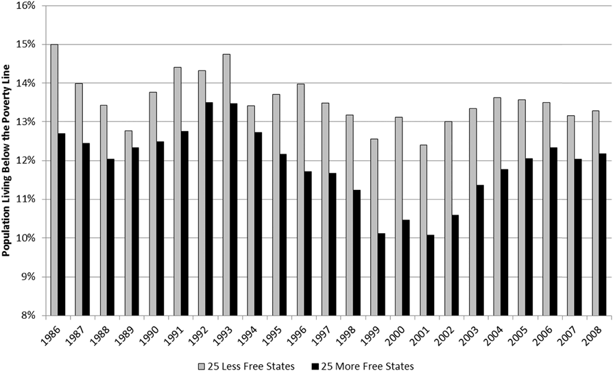
The average poverty rate among the more free states is lower than the average poverty rate among the less free states in every year in the sample, averaging 1.6 percentage points lower in the more free states (Figure 5). The greatest differences exceeded 2 percentage points in 1986, 1996, and 1999 through 2003. The smallest difference was less than half a percentage point in 1989.Footnote 22
Average poverty rates for the least and more free states as measured by the EFNA index.Footnote 21
C. Income inequalityFootnote 23
A criticism of poverty rates is that they can hide income inequality. For example, if many households earn just slightly more than the poverty level income while a small number of households earn tremendous incomes, the data would show zero poverty. Yet the zero poverty rate would give us no clue as to the existence of tremendous income inequality.
As James Madison said in Federalist 10, the equality of opportunity that Thomas Jefferson claimed was every human’s birthright will inevitably lead to inequality of outcome. As obvious as this was to Madison and Jefferson, though, “income inequality” has become a point of contention among academics and politicians alike. In the face of data showing that economic freedom is associated with higher income levels, less unemployment, and less poverty, the reasonable rejoinder is that those improvements must come at a cost of tremendous income disparity.
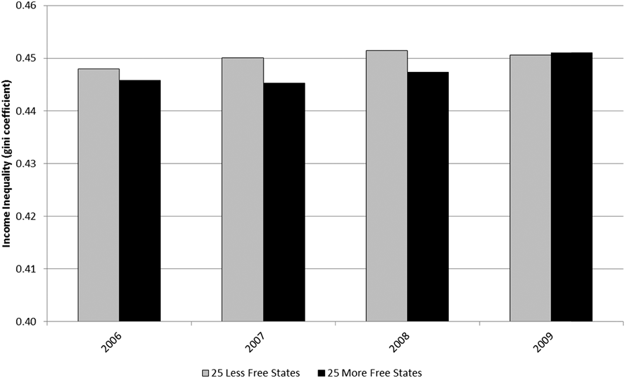
A comparison of the Gini coefficients for the more free and less free states is telling (Figure 6). Over the period for which the Census Bureau calculated the coefficients, the more free states exhibited less income inequality than the less free states in three out of four years, and in the fourth year the difference was almost zero.Footnote 24 The reduced income inequality among the more free states is not statistically significant, however. Be that as it may, the conventional claim is that income inequality is an inevitable byproduct of free markets. But the fact that income inequality is lower in the more free states, even though the difference is statistically zero, is sufficient evidence to rebut the claim.Footnote 25
Average income inequality measures for the least and more free states as measured by the EFNA index.Footnote 26
Income inequality measures suffer from well-known defects, some of which Horwitz discusses in the opening sections of his essay in this volume. The manner in which the Gini coefficient (which measures statistical dispersion in order to represent income distribution), for example, assumes that people do not move between income categories. For example, if the bottom 20 percent of wage earners earned 5 percent of all income this year and 4 percent next year, the popular interpretation would be that the poor got poorer. In fact, it is possible (and even likely) that the bottom 20 percent of wage earners this year are not the same people as the bottom 20 percent of wage earners last year. Thus, the income inequality measure could rise because the poor got poorer, or because the rich got richer while the poor stayed the same, or because the poor got richer but the rich got richer faster, or because there was no pattern to who got richer and who got poorer, but people’s movements between income groups caused the inequality coefficient to rise by random chance.
A good demonstration of the shortcomings of the popular interpretation of the Gini coefficient is found by applying the inequality calculations to people’s ages. In 2000, the youngest 20 percent of Americans were, on average, 7.1 years old. By 2010, the youngest 20 percent of Americans were, on average, 6.9 years old. A simpleminded interpretation would have us conclude that the young got younger. Sadly, no one ever gets younger. Rather, the composition of the youngest 20 percent changed — some grew up and were no longer part of the youngest 20 percent and new people were born and entered the youngest 20 percent. In the third section of his essay in this volume, Horwitz provides a similar example using student grades. The important lesson from both examples is that it is possible for a group’s average metric (age, grade, income) to decline even if every individual’s metric has increased. What drives this apparent contradiction is the fact that the group is made up of different individuals at different points in time.Footnote 27
Finally, it might be the case that this is a moot discussion in any event. After all, the poor do not suffer from inequality; they suffer from poverty. To accept this argument is to render a discussion of Gini coefficients meaningless, but also to leave us unsatisfied since our hope was that the inequality measure would address criticisms of the poverty measure. If our base concern is not that some people are unequal but rather that some people cannot afford life necessities, then an alternative approach to looking at income is to look, as Horwitz does in the fourth section of his essay in this volume, at consumption of life necessities.
D. Percentage of uninsured peopleFootnote 28
Measuring the consumption of life necessities is complicated by the fact that the government provides many life necessities to the poor in the form of food stamps, subsidized housing, energy assistance programs, and refundable tax credits. When we measure consumption of life necessities, it is unclear whether we are capturing people’s abilities to afford the necessities or the fact that the government is providing these necessities. One possible exception is health insurance. Unlike food, housing, and energy, health insurance is largely both a life necessity and a discretionary purchase. The fraction of people who do not have health insurance presents an alternative proxy for actual poverty. Unlike the poverty rate, the uninsured rate is not dependent on an official definition. Also unlike the poverty rate, those who earn above but close to the poverty line can continue to show up in the data. The uninsured rate presents its own drawbacks — the government provides Medicaid to the poor (though principally to those whose income is below the poverty line); the uninsured rate will fluctuate based on people’s youth and health history, not only their ability to pay. Nonetheless, the uninsured rate provides an alternative view of poverty that complements the poverty rate.
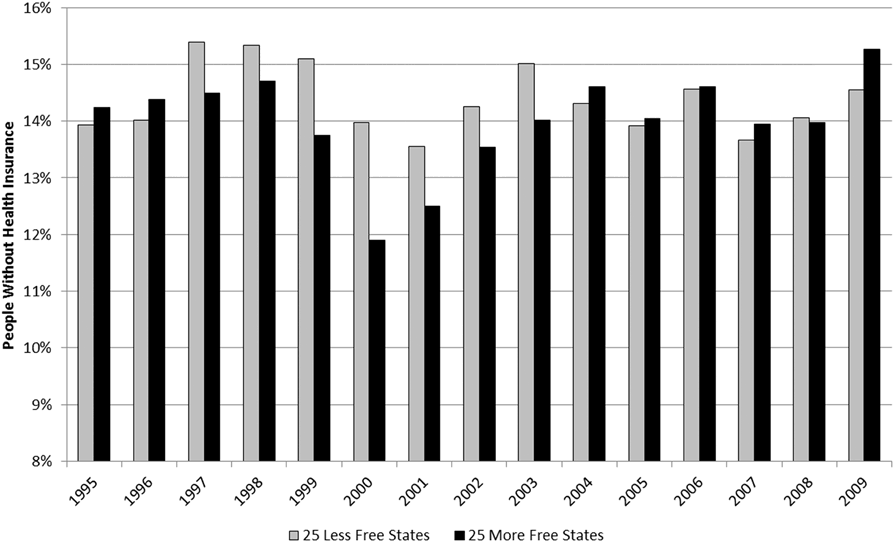
From 1995 through 2009, there were fewer uninsured people (per capita) in the more free states than in the less free states in eight out of the fifteen years (Figure 7). When the more free states experienced lower uninsured rates than the less free states, they did so by almost a full percentage point. Conversely, when the less free states experienced lower uninsured rates than the more free states, they did so by only a third of a percentage point. When citizens of the more free states have lower uninsured rates, the rates are much lower, but when citizens of the less free states have lower uninsured rates, the rates are only slightly lower.
Percentage of uninsured people in the least and more free states as measured by the EFNA index.Footnote 29
Overall, the average uninsured rate among the more free states was less than the uninsured rate among the less free states, though the difference was not statistically significant.Footnote 30
V. Population Growth
A. Population growth as a measure of socioeconomic healthFootnote 31
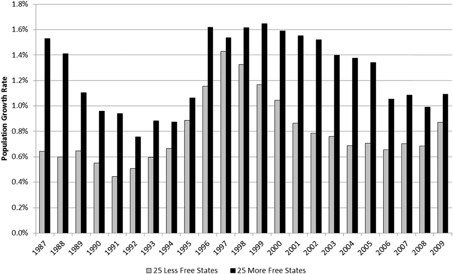
Over the sample period, the more free states experienced population growths that were almost 60 percent higher than those of the less free states (Figure 8). From 1987 through 2009, the more free states saw their populations grow (on average) by 1.3 percent annually versus 0.8 percent for the less free states. Compounding those growth rates over the twenty-three years in the sample means that the average more free state saw its population grow by one-third versus one-fifth for the average less free state.Footnote 32
Average annual population growth for the least and more free states as measured by the EFNA index.Footnote 33
A criticism is that population growth is not a very relevant measure of socioeconomic health and so may tell us nothing about the desirability of living in one group of states versus the other. For example, less-developed countries tend to have higher population growth rates than do developed countries, yet socioeconomic measures tend to be far better in developed countries. Of course, the comparison we examine here is not across countries but across states. Regardless, a measure that better captures people’s responses to differences in socioeconomic health across states is the migration ratio. While population growth rates only tell us that a population is growing, migration ratios can give us clues as to why.
B. In-migration relative to out-migration
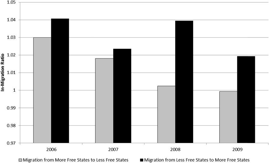
The IRS provides data going back to 2006 on between-state migration that show, for each combination of states, the number of people who changed their primary residence from one state in one year to a different state in the subsequent year. From this data, we construct the ratio of in-migrants to a state to out-migrants from that state, which yields what we term the “in-migration ratio.” For example, to say that “state A has an in-migration ratio of 1.1 relative to state B” means that (on average) 1.1 people moved from B to A for every 1 person who moved from A to B. Accounting for all pairwise combinations of states yields 1,225 in-migration ratios per year.
With respect to in-migration ratios, what is relevant is the freedom of the state into which the migrants are moving relative to the freedom of the state out of which the migrants are moving. We call this the “freedom ratio.” For example, to say that “state A has a freedom ratio of 1.1 relative to state B” means that state A’s freedom index is 1.1 times state B’s freedom index.
Over the sample period, the in-migration ratio for people moving from less free states to more free states averaged 1.03 while the in-migration ratio for people moving from more free states to less free states averaged 1.01 (Figure 9).Footnote 35 In other words, people migrate into more free states out of less free states at a higher rate than they migrate into less free out of more free states. These results suggest that people are voting with their feet. They are moving into more free states — and this is not merely movement from one free state to another free state. People are specifically moving out of less free states into more free states.
Average ratio of in-migrants to out-migrants for migrations between states of different freedoms as measured by the EFNA index.Footnote 34
VI. Fiscal Health of the Government
A. Tax revenue
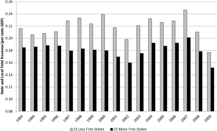
State and local government revenue is derived from taxes, licensing, intergovernmental sources, and non-tax and non-licensing activities such as utility revenue, liquor store revenue, and social insurance trust revenue.Footnote 36 State and local tax revenue is a component in the construction of the EFNA index, so it is not surprising (Figure 10) to find that more free states collected a significantly smaller share of GDP (18.1 percent) in tax revenue than did the less free states (21.9 percent).Footnote 37 What is surprising is that if we classify states only according to labor market freedom — a criterion that is not based on government revenue — we get similar results. State and local government revenue averages 18.2 percent of GDP among the states with the most labor market freedoms, but 21.8 percent among the states with the fewest labor market freedoms.Footnote 38 States that impose fewer restrictions on labor markets collect more tax revenue (as a fraction of GDP) than do states that impose more restrictions.
State and local government total revenue as a fraction of state GDP for the least and more free states as measured by the EFNA labor market freedom index.Footnote 39
B. Government debt relative to the size of the economyFootnote 40
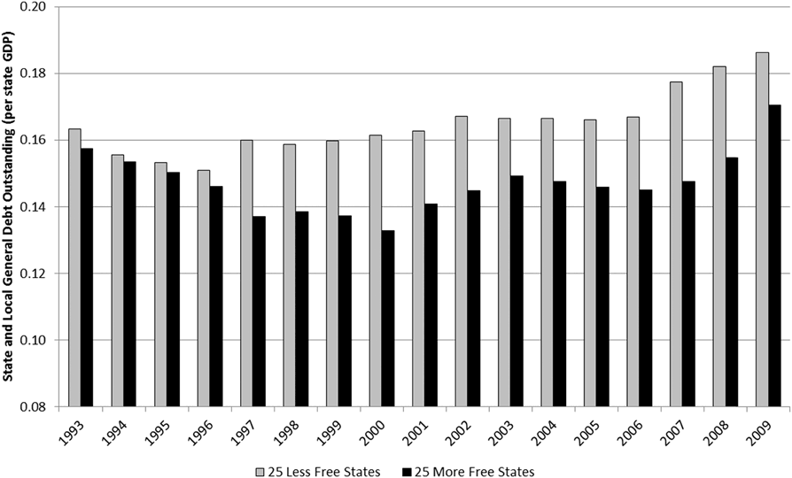
One might expect that, since the more free states collect a smaller share of the economy in tax revenue, those states would also exhibit greater debt levels due to deficit spending. This is not the case. On average, the more free states have state and local debt equal to 14.7 percent of their GDPs (Figure 11). The less free states have debt loads equal to 16.5 percent of their GDPs.Footnote 41 As the average state GDP is $300 billion, the 1.8 percentage point difference is the equivalent of $5.3 billion in additional debt for the average less free state.
State and local general debt outstanding for the least and more-free states as measured by the EFNA index.Footnote 42
A reasonable counterargument is that the more free states have lesser debt loads not because they have more financially efficient governments, but simply because their governments are smaller. A smaller government means less debt but it also means less ability to provide public services. This may be true. However, the point of public services is not the services but the improved quality of life those services make possible. We have already seen that poverty rates are lower in the more free states, unemployment is lower, incomes are higher, equality is somewhat greater (and certainly not worse), and the uninsured rate is mostly lower. More importantly, migration data show that people are moving out of less free states into more free states. Consequently, even if it were true that more free states only have lower debt loads because they provide fewer public services, other metrics suggest that quality of life is not worse because of it.
VII. Economic Growth
A. Growth in the number of firmsFootnote 43
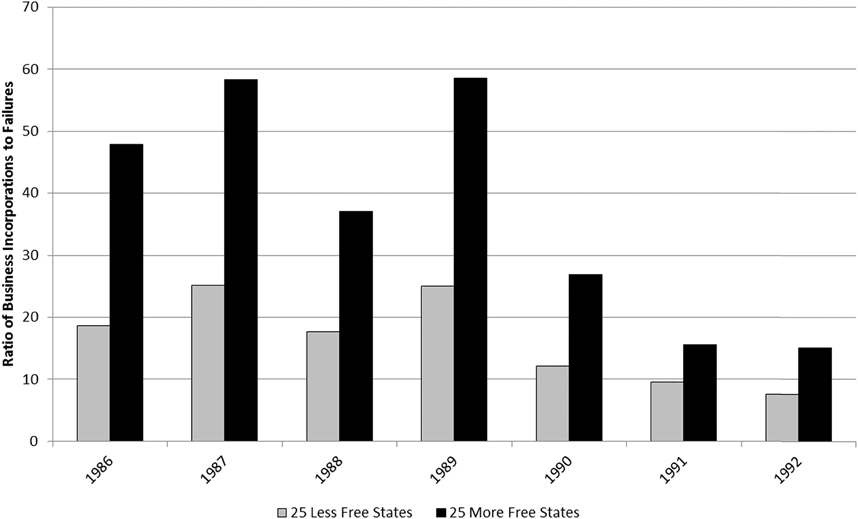
Prior to 1993, the Census Bureau recorded the number of business incorporations and closures in each state. There is then a break in the Census data and the series resumes, recast as “business births and deaths,” in 2003. Of course, one would expect that larger economies would have more firm births and deaths. What is important is the ratio of the births to the deaths within the states. For example, a birth to death ratio of 10 indicates that ten new firms are founded for every one firm that closes. From 1986 to 1992, the ratio of business incorporations to closures averaged 16.5 for the less free states and 37.0 for the more free states (Figure 12). Corporations were being created (in a net sense) in the more free states at more than twice the rate as in the less free states.Footnote 44
Ratio of business incorporations to business closures for the least and more free states as measured by the EFNA index.Footnote 45
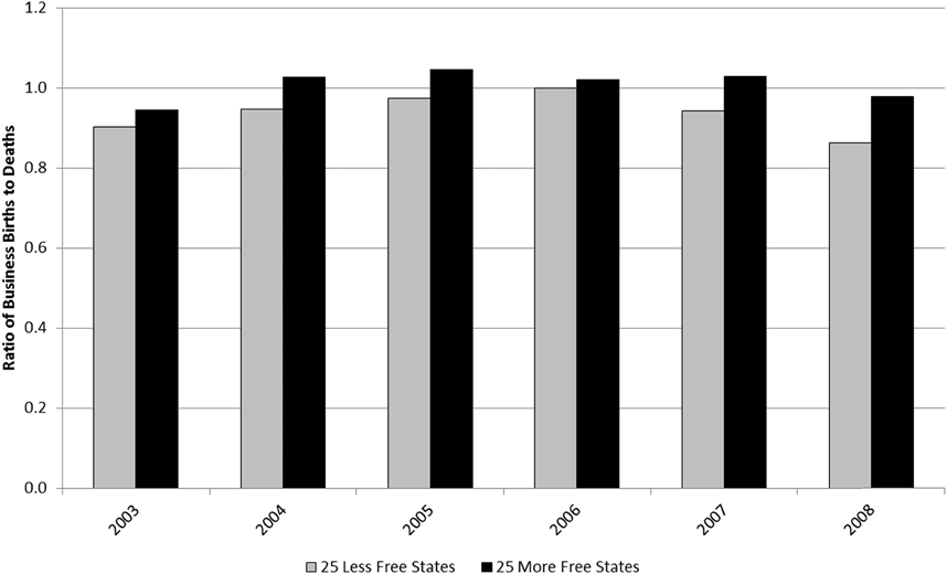
From 2003 to 2008, the ratio of business births to deaths was 1.7 for the more free states and 1.4 for the less free states (Figure 13).Footnote 47 The underlying assumption is that a higher birth to death ratio is good because it indicates more new businesses arriving offering new or better products, more opportunities for employment, and more opportunities for entrepreneurship. Of course, not all new businesses offer better products. It is possible that a state could show a high birth to death ratio due to the founding of many new firms that offer inferior products at higher prices. However, new businesses that offer worse products will tend to fail, ultimately resulting in a reduced birth to death ratio. Consequently, while a flood of new firms offering inferior products can boost the birth to death ratio in a given year, we would expect to see a counterbalancing decline in the birth to death ratio in subsequent years as consumers reject the new and inferior products. Yet what we see in the data is a pattern of continued high birth to death ratios for the more free states, indicating that old firms that produced superior products are not being replaced by new firms that produce inferior products.
Ratio of business births to business deaths for the least- and more free states as measured by the EFNA index.Footnote 46
Another reasonable counterargument is that a change in the number of firms says nothing about the change in the sizes of the firms. For example, gaining ten new firms for every one closed firm will mean fewer jobs if each of the ten new firms employs five people whereas the one closed firm employed five hundred. Yet we have already seen that the unemployment rate is lower among the more free states. This suggests that the higher birth to death ratio in the more free states is not coming at the cost of small firms replacing large firms.
B. Growth in state GDPFootnote 48
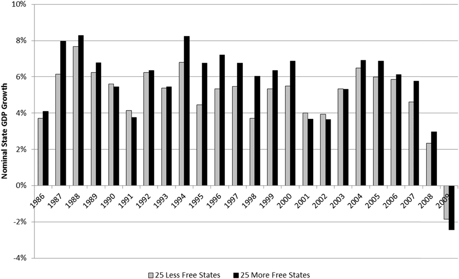
If state and local governments in the more free states collect a smaller share of the economy in tax revenue, then spending in those states would also be more constrained. And if the general Keynesian observation that state and local governments enhance aggregate demand, which in turn should drive economic growth, then GDP growth in those more free states should be lower. But this is not the case. Average annual GDP growth among the more free states is a full percentage point higher than for the less free states. Over the period 1986 through 2009, the economies of the more free states grew at an average nominal rate of 5.8 percent versus 4.8 percent for the less free states (Figure 14).Footnote 49 A state economy that grows one percentage point faster per year will, over the course of a decade, end up 10 percent larger than it would otherwise. For the average state, this is the equivalent of an additional 30 billion dollars in economic activity.
State GDP growth for the least and more free states as measured by the EFNA index.Footnote 50
VIII. Prosperity
Given the randomness of time, place, circumstances of birth, and specific events, economic freedom is the best approximation of equality of opportunity humans can hope to achieve. Across time and across states, data show that more economic freedom is correlated with improved socioeconomic outcomes. That is, economic freedom and prosperity tend to go hand-in-hand. And this prosperity is not limited to the rich but permeates all strata of society. In the presence of economic freedom, median incomes are higher, unemployment is lower, poverty is lower, the likelihood of being uninsured is lower, the public fisc is more sound, and entrepreneurship is more robust. Even if this were all that economic freedom had to offer, we might be hard-pressed to justify trading-off this bounty for greater equality of outcome. Yet the data also show that economic freedom goes hand-in-hand with greater income equality. This is not to say that economic freedom somehow promotes equality of outcome. So long as people are born with different talents and under different circumstances, economic freedom will guarantee inequality of outcome. What the data do suggest is that economic freedom promotes less inequality of outcome than do systems that repress economic freedom. Where practical economic choices are concerned, what matters is not the comparison of economic freedom to the ideal, but to the alternative. According to the data, the alternative to economic freedom not only attains less equality of opportunity, it also attains less equality of outcome and a lower level of outcome.