

1. Introduction
Thermally driven convection is ubiquitous in nature and industrial processes. Rayleigh–Bénard convection (RBC) is a classical paradigm to study such phenomenon, in which buoyancy-driven flow is induced in a pure fluid layer due to heating from below and cooling from above. RBC has been studied extensively in past decades (Siggia Reference Siggia1994; Ahlers, Grossmann, & Lohse Reference Ahlers, Grossmann and Lohse2009; Lohse & Xia Reference Lohse and Xia2010; Chillà & Schumacher Reference Chillà and Schumacher2012) due to the omnipresence of buoyancy-driven convection in nature and technology. Two dimensionless parameters are standardly used to characterise RBC: (i) pure-fluid Rayleigh number (Raf) which describes the ratio of buoyant to viscous forces and (ii) Prandtl number (Pr) which is the ratio of momentum and thermal diffusivity. A third parameter,  $\varGamma$, defines the aspect ratio of the convection cell. The main response of the system is the fluidic Nusselt number (Nuf), which describes the efficiency of heat transfer and is defined as the ratio of the total heat transfer rate (conduction and convection) to the conductive heat transfer rate at a wall surface. For very high Rayleigh numbers, there exists an asymptotic regime, where the relationship between Raf and Nuf can typically be described through a constant power law. Considerable literature has been devoted to studying this regime, including several numerical (Toppaladoddi, Succi, & Wettlaufer Reference Toppaladoddi, Succi and Wettlaufer2017; Zhu et al. Reference Zhu, Stevens, Verzicco and Lohse2017, Reference Zhu, Mathai, Stevens, Verzicco and Lohse2018; Iyer et al. Reference Iyer, Scheel, Schumacher and Sreenivasan2020; Li et al. Reference Li, He, Tian, Hao and Huang2021) and experimental (Niemela et al. Reference Niemela, Skrbek, Sreenivasan and Donnelly2000; Roche et al. Reference Roche, Castaing, Chabaud and Hebral2001; He et al. Reference He, Funfschilling, Bodenschatz and Ahlers2012a,Reference He, Funfschilling, Nobach, Bodenschatz and Ahlersb; Zhang et al. Reference Zhang, Sun, Bao and Zhou2018; Tummers & Steunebrink Reference Tummers and Steunebrink2019) studies.
The analogous problem of thermally (also solutally) driven convection in porous media has begun to receive increasing attention due to its prevalence in assorted domains. Some well-known examples include heat transfer in volcanic rock systems (Ratouis & Zarrouk Reference Ratouis and Zarrouk2016), subseafloor thermohaline convection (Wilson & Ruppel Reference Wilson and Ruppel2007), sequestration of carbon dioxide (Cinar, Riaz, & Tchelepi Reference Cinar, Riaz and Tchelepi2009; Hassanzadeh, Pooladi-Darvish, & Keith Reference Hassanzadeh, Pooladi-Darvish and Keith2012; De Paoli, Zonta, & Soldati Reference De Paoli, Zonta and Soldati2016), and hydrothermal convection needed for extraction of geothermal energy (Gasparini & Mantovani Reference Gasparini and Mantovani1984). Several experimental, analytical, and numerical studies (Jonsson & Catton Reference Jonsson and Catton1985; Kladias & Prasad Reference Kladias and Prasad1991; Otero et al. Reference Otero, Dontcheva, Johnston, Worthing, Kurganov, Petrova and Doering2004; Hewitt, Neufeld, & Lister Reference Hewitt, Neufeld and Lister2012, Reference Hewitt, Neufeld and Lister2013, Reference Hewitt, Neufeld and Lister2014; Keene & Goldstein Reference Keene and Goldstein2015; Wen, Corson, & Chini Reference Wen, Corson and Chini2015; Liang et al. Reference Liang, Wen, Hesse and DiCarlo2018; Hewitt Reference Hewitt2020; Liu et al. Reference Liu, Jiang, Chong and Zhu2020) have been devoted to characterising the corresponding convective behaviour and its governing parameters. Like that of RBC, a Rayleigh–Darcy number, commonly referred to as just the Rayleigh number (Ra), is typically used instead as the governing parameter and studied in relation to a porous medium Nusselt (Nu) number. Conventionally, five regimes have been used to describe this type of convection as a function of Ra (Nield & Bejan Reference Nield and Bejan2017):
I. the conduction-only regime [0 ≤ Ra ≤ 4
 ${\rm \pi}$2];
II. the steady-state regime [4
${\rm \pi}$2 ≤ Ra ≤ 350];III. the quasi-periodic regime [350 ≤ Ra ≤ 1300];
IV. the high-Rayleigh-number regime [1300 ≤ Ra ≤ 10 000], a turbulent regime that lacks large coherent structures; and
V. the ultimate Rayleigh regime [Ra > 10 000], similar to the high-Rayleigh-number regime but differing in that the inner flow field becomes self-organised with an interior mega-plume region separated by thin micro-plumic regions close to the bounding wall.


Experiments by Keene and Goldstein (Reference Keene and Goldstein2015) and Kladias and Prasad (Reference Kladias and Prasad1991) have further shown that a constant power law regime is present in porous convection at very high Ra, suggesting that the presence of the solid phase appears to be nullified. Various authors have suggested power law relationships between Nu and Ra in the form  $Nu \propto R{a^b}$ for this regime, where b is a constant scaling exponent. Based on experiments with compressed argon and polypropylene spheres, Keene and Goldstein proposed b = 0.319 for Ra > 7470. Lister (Reference Lister1990) studied convection with water and carbon fibres, suggesting a scaling exponent of 0.33 for high Ra. Davidson, Kulacki, and Savela (Reference Davidson, Kulacki and Savela2009) performed experiments on a water-saturated carbon foam. They also included the Prandtl number and the ratio of effective-to-fluid thermal conductivity, km/kf, in their Nu–Ra relation as
 $Nu = (0.008 \pm 0.003){({k_m}/{k_f})^{0.25 \pm 0.04}}R{a^{0.50 \pm 0.02}}P{r^{0.38 \pm 0.04}}$. It is also pointed out that the magnitude of Nu from the above-mentioned experiments have been quite scattered, varying up to an order of magnitude at some Rayleigh numbers.
Up to this point, theoretical and numerical studies for porous media convection have largely relied on macroscopic models; in particular, the Darcy–Oberbeck–Boussinesq (DOB) equations (Nield & Bejan Reference Nield and Bejan2017) have been widely adopted for both thermal and solutal convection. In contrast to experimental studies, Nu–Ra relations obtained from these macroscopic models predict much higher scaling exponents in the range of 0.9–0.95. Otero et al. (Reference Otero, Dontcheva, Johnston, Worthing, Kurganov, Petrova and Doering2004) used the DOB equations to develop a fit of  $Nu \propto R{a^{0.90}}$. Hewitt et al. (Reference Hewitt, Neufeld and Lister2012) performed simulations based on the DOB equations up to
 $Ra= 50\ 000 $. They recommended b = 0.95 as a scaling exponent. Using the same formulation, Kränzien and Jin (Reference Kränzien and Jin2018) found that a simple linear fit may be more appropriate as
 $Nu = 0.076Ra + 0.935$. Although sparse, some authors have studied thermal and solutal convection in the presence of a porous medium with pore-resolved direct numerical simulations (DNS). Liu et al. (Reference Liu, Jiang, Chong and Zhu2020) recently performed a two-dimensional (2-D) DNS of thermal convection in a square domain with circular objects. They showed that the relationship between Nu and the porosity ϕ was non-monotonic due to the interplay of two competing forces: an increase in heat transfer due to the flow coherence vs. an increase in flow impedance with the addition of the solid array. They also demonstrated asymptotic behaviour of Nu at high Ra numbers, suggesting a relation based on the unconfined fluid Rayleigh and Nusselt number:
 $N{u_f} \propto Ra_f^{0.30}$. Their results presented on the Nu–Ra scale matched well with the b = 0.319 scaling coefficient by Keene and Goldstein (Reference Keene and Goldstein2015), however, the magnitude of Nu did not show as large of a variance as demonstrated by experiments. A possible reason for this is that Liu et al. only considered a special case with solid-to-fluid thermal conductivity ratio ks/kf = 1, while in the experiments by Keene and Goldstein (Reference Keene and Goldstein2015) and Kladias and Prasad (Reference Kladias and Prasad1991) it ranged from approximately 0.33 up to around 321.
A few authors have also directly compared pore-resolved DNS with results obtained from the DOB equations. Karani and Huber (Reference Karani and Huber2017) performed such a comparison for heat transfer at low Rayleigh numbers (Ra < 200), finding that the DOB equations were not able to capture the onset of convection when ks/kf ≠ 1. Gasow et al. (Reference Gasow, Lin, Zhang, Kuznetsov, Avila and Jin2020) recently performed a numerical comparison between the DOB equations and pore-resolved DNS for mass transfer. They found that the boundary layer thickness was determined by the pore size instead of the Rayleigh number, and that DNS results predicted a nonlinear scaling between the Sherwood and Rayleigh number (analogous to Nu–Ra for heat transfer). They concluded that ‘pore-scale parameters’ not captured in the DOB equations played a large role in the convection dynamics, thus suggesting the need for an extension or improvement of the standard DOB equations. Although focused on mass transfer, Gasow et al. noted that similar investigation is needed for heat transfer due to the addition of conjugate heat transfer between fluid and solid phases, which was absent in their study. To the best of the authors’ knowledge, a comparison of DOB simulations and DNS for thermal convection in porous media with differing thermal transport properties in each phase for high Ra (above 200) has not been performed. With the large variation in results obtained with the DOB equations and those from pore-resolved simulations and experiments, two questions arise.
(1) Under what range of conditions are the assumptions used in deriving the DOB equations valid for thermal convection?
(2) To what extent do conjugate heat transfer and pore size affect the dynamics of thermal convection at higher Ra?
Thus, the objective of this study is to answer these questions by performing pore-resolved DNS on a simplified 2-D domain and compare with results from corresponding DOB simulations. We exclusively use the lattice Boltzmann method (LBM) for all simulations, considering Rayleigh numbers up to 50 000.
It is noted that while an actual physical system is, in fact, three-dimensional (3-D), due to the requirement of high resolution and the need to study a wide range of parameters, we employ a simplified 2-D configuration. A detailed investigation by van der Poel, Stevens, and Lohse (Reference van der Poel, Stevens and Lohse2013) for RBC found that 2-D and 3-D simulations predicted similar Nusselt numbers for high Pr. Hewitt et al. (Reference Hewitt, Neufeld and Lister2014) also performed 3-D simulations using the DOB equations, finding that Nu was approximately 40% larger at high Ra in three dimensions when compared with 2-D results. Nonetheless, the scaling coefficient that best fit 3-D data was reported as 0.94, compared with 0.95 from 2-D simulations performed by the same group. While some discrepancy is expected between 2-D and 3-D results, we expect the dynamics observed in 2-D simulations to be comparable and conclusions made regarding the comparison of DNS and DOB simulations to be valid for 3-D cases.
The remainder of this paper is organised as follows. The mathematical formulation for both pore-resolved and macroscopic models are described in detail in § 2, and the corresponding numerical methods in § 3. The validation of the numerical models is shown in § 4. We then present the simulation results in § 5, focusing on the effects of pore size, conjugate heat transfer and porosity on the plume dynamics, flow structure, Nu–Ra relations and boundary layer thickness. We summarise our findings and discuss future work in § 6. Appendices A and B provide additional information on numerical validation and instantaneous temperature fields, respectively, while the supplementary movies are available at https://doi.org/10.1017/jfm.2022.491 showing the evolution of the temperature fields from the specified initial conditions to statistically steady states for both representative DOB and DNS results.
2. Mathematical formulation
2.1. Pore-scale DNS
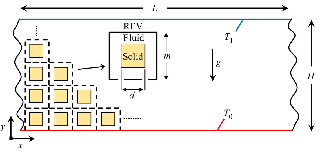
We consider a 2-D fluid saturated porous medium with square solid blocks as shown in figure 1. The enclosure has an aspect ratio,  $\varGamma$, of 2 where
 $\varGamma$ = Length(L)/Height(H). The dimensions of the blocks are d × d and the representative elementary volume (REV) has size m × m. The porosity of the domain, ϕ, is uniquely determined by the ratio d/m as
 \begin{equation}\phi = 1 - {\left( {\frac{d}{m}} \right)^2}.\end{equation}
For this work, we consider three REV sizes as H/m = 10, 25 and 50. It is pointed out that varying H/m (at a fixed ϕ) is representative of varying the pore size within the medium (Gasow et al. Reference Gasow, Lin, Zhang, Kuznetsov, Avila and Jin2020). The Boussinesq fluid is heated from below and cooled from above with temperatures T 0 and T 1 at the bottom and top walls, respectively. Periodic boundary conditions are employed on the vertical sides for both the flow and thermal field, and no-slip boundary conditions are imposed on all solid surfaces. Conjugate heat transfer is considered at the fluid–solid interface of the square blocks as
 \begin{gather}{T_f} = {T_s},\end{gather}
 \begin{gather}\boldsymbol{n}\boldsymbol{\cdot }{(k\boldsymbol{\nabla }T)_f} = \boldsymbol{n}\boldsymbol{\cdot }{(k\boldsymbol{\nabla }T)_s},\end{gather}
where T is the temperature, k the thermal conductivity, the f and s subscripts denote the fluid and solid phases, respectively, and n is the unit normal vector to the fluid–solid interface.
Schematic of porous domain used in direct numerical simulations.

For the fluid phase, the governing equations for DNS are the Navier–Stokes equations (using the Boussinesq approximation) and the energy equation:
 \begin{gather}\boldsymbol{\nabla }\boldsymbol{\cdot }\boldsymbol{u} = 0,\end{gather}
 \begin{gather}{\partial _t}(\boldsymbol{u}) + (\boldsymbol{u}\boldsymbol{\cdot }\boldsymbol{\nabla })\boldsymbol{u} ={-} \frac{1}{\rho }\boldsymbol{\nabla }P + {\nu _f}{\nabla ^2}(\boldsymbol{u}) + \boldsymbol{g}\beta (T - {T_{ref}}),\end{gather}
 \begin{gather}{(\rho {c_p})_f}{\partial _t}({T_f}) + \boldsymbol{\nabla }\boldsymbol{\cdot }[{(\rho {c_p})_f}\boldsymbol{u}{T_f}] = \boldsymbol{\nabla }\boldsymbol{\cdot }({k_f}\boldsymbol{\nabla }{T_f}),\end{gather}
where u is the velocity vector, ρ the density, P the pressure, ν the kinematic viscosity, g the gravitational vector, β the thermal expansion coefficient, Tref a reference temperature taken as Tref = (T 0 + T 1)/2 and cp the specific heat. For the solid phase, the energy equation reduces to
 \begin{equation}{(\rho {c_p})_s}{\partial _t}({T_s}) = \boldsymbol{\nabla }\boldsymbol{\cdot }({k_s}\boldsymbol{\nabla }{T_s}).\end{equation}
Using the reference length H, reference velocity uref = gβΔTK/ν, reference time tref = H/uref, and characteristic temperature difference ΔT = T 0–T 1 (2.4)–(2.7) can be written in dimensionless form as
 \begin{gather}\tilde{\boldsymbol{\nabla}}\boldsymbol{\cdot }\tilde{\boldsymbol{u}} = 0,\end{gather}
 \begin{gather}{\partial _{\tilde{t}}}(\tilde{\boldsymbol{u}}) + (\tilde{\boldsymbol{u}}\boldsymbol{\cdot }\tilde{\boldsymbol{\nabla }})\tilde{\boldsymbol{u}} ={-} \tilde{\boldsymbol{\nabla }}\tilde{P} + \frac{{Pr}}{{R{a_f}Da}}{\tilde{\boldsymbol{\nabla }}^2}(\tilde{\boldsymbol{u}}) + \frac{{Pr}}{{R{a_f}D{a^2}}}{z_i}\tilde{T},\end{gather}
 \begin{gather}{\partial _{\tilde{t}}}({\tilde{T}_f}) + \tilde{\boldsymbol{\nabla }}\boldsymbol{\cdot }(\tilde{\boldsymbol{u}}{\tilde{T}_f}) = \frac{1}{{R{a_f}Da}}{\tilde{\nabla }^2}({\tilde{T}_f}),\end{gather}
 \begin{gather}{\partial _{\tilde{t}}}({\tilde{T}_s}) = \frac{\gamma }{{R{a_f}Da}}{\tilde{\nabla }^2}({\tilde{T}_s}),\end{gather}
where  ${}^{\sim}$ denotes a dimensionless value,
 $\tilde{\boldsymbol{\nabla }} = H\boldsymbol{\nabla }$,
 $\tilde{T} = T/\varDelta T$ and the following dimensionless variables are defined:
 \begin{equation}\left.
\begin{gathered} {Pr =
\dfrac{{{\nu_f}}}{{{\alpha_f}}},\quad R{a_f} =
\dfrac{{{H^3}\beta \Delta Tg}}{{{\nu_f}{\alpha_f}}},\quad
Da = \dfrac{K}{{{H^2}}},\quad \alpha = \dfrac{k}{{\rho
{c_p}}}}\\ {\textrm{ }\sigma = \dfrac{{{{(\rho
{c_p})}_s}}}{{{{(\rho {c_p})}_f}}},\quad \gamma =
\dfrac{{{\alpha_s}}}{{{\alpha_f}}},\quad \textrm{and}\quad
\dfrac{{{k_s}}}{{{k_f}}} = \gamma \sigma } \end{gathered}\right\},\end{equation}
where Pr is the Prandtl number, Raf the Rayleigh number for unconfined fluid flow, Da the Darcy number, K the permeability, σ the heat capacity ratio and γ the thermal diffusivity ratio. It should be noted that while only γ is present in the governing equations (2.8)–(2.11), the conductivity ratio k s/k f shows up in the conjugate conditions (2.2) and (2.3). We define the Nusselt number as the ratio of total heat transfer rate (convective and conductive),  ${{\dot{Q}}_{total}}$, to purely conductive heat transfer rate,
 ${{\dot{Q}}_{cond}}$, at statistically steady state on the wall as
 \begin{equation}Nu =
\frac{{{{\dot{Q}}_{total}}}}{{{{\dot{Q}}_{cond}}}} =
\dfrac{{\displaystyle\int_w {k\overline {\dfrac{{\partial
\tilde{T}}}{{\partial \tilde{y}}}\,} \textrm{d}A}
}}{{\displaystyle\int_w {{{\left. {\left( {k\overline
{\dfrac{{\partial \tilde{T}}}{{\partial \tilde{y}}}\,}
\textrm{d}A} \right)} \right|}_{R{a_f} = 0}}}
}},\end{equation}
where the subscript w represents either the top or bottom wall and the  ${}^{-}$ symbol denotes the time-averaged value.
2.2. Continuum-scale DOB equations
For the continuum scale, we begin with volume-averaging of (2.4) and (2.5) following the ‘Brinkman-Forchheimer’ equation of Nield and Bejan (Reference Nield and Bejan2017) for an incompressible fluid with the buoyancy force represented by the Boussinesq approximation:
 \begin{gather}\boldsymbol{\nabla }\boldsymbol{\cdot }(\phi \langle \boldsymbol{u}\rangle ) = 0,\end{gather}
 \begin{gather}\begin{aligned} &
{\partial _t}(\phi \langle \boldsymbol{u}\rangle ) +
\boldsymbol{\nabla }\boldsymbol{\cdot }(\phi \langle
\boldsymbol{\mathord{\buildrel{\lower3pt\hbox{$\scriptscriptstyle\smile$}}
\over u}
\mathord{\buildrel{\lower3pt\hbox{$\scriptscriptstyle\smile$}}
\over u} }\rangle ) + \phi \langle \boldsymbol{u}\rangle
\boldsymbol{\cdot }\boldsymbol{\nabla }\langle
\boldsymbol{u}\rangle ={-} \nabla \phi \langle P\rangle \\
& \quad + {\nu _f}{\nabla ^2}(\phi \langle
\boldsymbol{u}\rangle ) + \phi \boldsymbol{g}\beta (\langle
T\rangle - {T_{ref}}) - \dfrac{{{\phi ^2}{\nu
_f}}}{K}\langle \boldsymbol{u}\rangle - \dfrac{{{\phi
^3}{c_F}\rho }}{{\sqrt K }}|\langle \boldsymbol{u}\rangle
|\langle \boldsymbol{u}\rangle .
\end{aligned}\end{gather}
The last two terms in (2.15) denote the Darcy and Forchheimer drag components and  $\boldsymbol{\nabla }\boldsymbol{\cdot }(\phi \langle \boldsymbol{\mathord{\buildrel{\lower3pt\hbox{$\scriptscriptstyle\smile$}} \over u} \mathord{\buildrel{\lower3pt\hbox{$\scriptscriptstyle\smile$}} \over u} }\rangle )$ denotes the momentum dispersion. The drag terms appear from the volume-averaging process (de Lemos Reference de Lemos2012) and represent the total drag force per unit volume due to the existence of the porous medium. The
 $\langle \cdot \rangle $ symbol represents volume-averaged quantities and the ̌ symbol denotes the fluctuating fields with respect to the averaged value of the local field for the fluid phase (Karani et al. Reference Karani, Rashtbehesht, Huber and Magin2017; Gasow et al. Reference Gasow, Lin, Zhang, Kuznetsov, Avila and Jin2020). It is noted here that the above is equivalent to the formulation in Gasow et al. (Reference Gasow, Lin, Zhang, Kuznetsov, Avila and Jin2020). Under the assumption of local thermal equilibrium, the volume-averaged energy balance equation becomes
 \begin{equation}{(\rho {c_p})_m}{\partial _t}(\langle T\rangle ) + {(\rho {c_p})_f}\boldsymbol{\nabla }\boldsymbol{\cdot }(\phi \langle \boldsymbol{u}\rangle \langle T\rangle ) + {(\rho {c_p})_f}\boldsymbol{\nabla }\boldsymbol{\cdot }(\phi {\langle \boldsymbol{\mathord{\buildrel{\lower3pt\hbox{$\scriptscriptstyle\smile$}} \over u} }\mathord{\buildrel{\lower3pt\hbox{$\scriptscriptstyle\smile$}} \over T} \rangle ^f}) = {k_m}{\nabla ^2}\langle T\rangle ,\end{equation}
where km is an effective thermal conductivity, (ρcp)m is the overall specific heat capacity with  ${(\rho {c_p})_m} = \phi {(\rho {c_p})_f} + (1 - \phi ){(\rho {c_p})_s}$ and
 ${(\rho {c_p})_f}\boldsymbol{\nabla }\boldsymbol{\cdot }(\phi {\langle \boldsymbol{\mathord{\buildrel{\lower3pt\hbox{$\scriptscriptstyle\smile$}} \over u} }\mathord{\buildrel{\lower3pt\hbox{$\scriptscriptstyle\smile$}} \over T} \rangle ^f})$ is the thermal dispersion term (Karani et al. Reference Karani, Rashtbehesht, Huber and Magin2017; Gasow et al. Reference Gasow, Lin, Zhang, Kuznetsov, Avila and Jin2020). The
 ${\langle \cdot \rangle ^f}$ operator (with superscript f) denotes volume-averaging over only the fluid phase. Assuming that thermal dispersion and momentum dispersion are negligible and introducing the additional dimensionless variables
 \begin{equation}Ra = \frac{{H\beta \Delta TgK}}{{{\nu _f}{\alpha _m}}},\quad \zeta = \frac{{{\alpha _m}}}{{{\alpha _f}}},\quad \bar{\phi } = \frac{{{{(\rho {c_p})}_m}}}{{{{(\rho {c_p})}_f}}} = \phi + (1 - \phi )\sigma .\end{equation}
Equations (2.14)–(2.16) can be rewritten as
 \begin{gather}\hat{\boldsymbol{\nabla }}\boldsymbol{\cdot }\hat{\boldsymbol{u}} = 0,\end{gather}
 \begin{gather}{\partial _{\hat{t}}}(\hat{\boldsymbol{u}}) + \hat{\boldsymbol{u}}\boldsymbol{\cdot }\hat{\boldsymbol{\nabla }}(\hat{\boldsymbol{u}}/\phi ) ={-} \frac{1}{\rho }\hat{\boldsymbol{\nabla }}\phi \hat{P} + \frac{{Pr}}{{\zeta Ra}}{\hat{\nabla }^2}(\hat{\boldsymbol{u}}) + \frac{{\phi \,Pr}}{{\zeta RaDa}}\hat{T}{z_i} - \frac{{\phi \,Pr}}{{\zeta RaDa}}\hat{\boldsymbol{u}} - \frac{{\phi {c_F}}}{{\sqrt {Da} }}|\hat{\boldsymbol{u}}|\hat{\boldsymbol{u}},\end{gather}
 \begin{gather}{\partial _{\hat{t}}}(\hat{T}) + \hat{\boldsymbol{\nabla } }\boldsymbol{\cdot }\left( {\frac{{\hat{\boldsymbol{u}}\hat{T}}}{{\bar{\phi }}}} \right) = \frac{1}{{Ra}}{\hat{\nabla }^2}(\hat{T}),\end{gather}
where  $Ra = R{a_f}Da/\zeta$ is the Rayleigh number for the porous medium,
 ${\alpha _m} = {k_m}/{(\rho {c_p})_m}$ the effective thermal diffusivity, ζ the ratio between αm and αf,
 $\bar{\phi }$ the ratio between the overall heat capacity and that of the fluid and zi is the ith component of the unit vector in the gravity direction. The symbol ̂ represents dimensionless volume-averaged quantities and
 $\hat{\boldsymbol{u}} = \phi \langle \boldsymbol{u}\rangle$ is the superficial velocity (also called Darcy velocity). With the assumption that
 $Da \ll 1$, the DOB equations are obtained:
 \begin{gather}\hat{\boldsymbol{\nabla } }\boldsymbol{\cdot }\hat{\boldsymbol{u}} = 0,\end{gather}
 \begin{gather}\hat{\boldsymbol{\nabla }}{\hat{P}_n} ={-} \hat{\boldsymbol{u}} + {z_i}\hat{T},\end{gather}
 \begin{gather}{\partial _{\hat{t}}}\hat{T} + \hat{\boldsymbol{\nabla } }\boldsymbol{\cdot }\left( {\frac{{\hat{\boldsymbol{u}}\hat{T}}}{{\bar{\phi }}}} \right) = \frac{1}{{Ra}}{\hat{\nabla }^2}\hat{T},\end{gather}
where  ${\hat{P}_n} = RaDa\langle p\rangle /\zeta Pr$ is a normalised pressure. Equations (2.21)–(2.23) are the same as the traditional DOB equations used for macroscopic-level studies (Otero et al. Reference Otero, Dontcheva, Johnston, Worthing, Kurganov, Petrova and Doering2004; Hewitt et al. Reference Hewitt, Neufeld and Lister2012, Reference Hewitt, Neufeld and Lister2013, Reference Hewitt, Neufeld and Lister2014; Wen et al. Reference Wen, Corson and Chini2015; Karani & Huber Reference Karani and Huber2017; Nield & Bejan Reference Nield and Bejan2017; Kränzien & Jin Reference Kränzien and Jin2018; Gasow et al. Reference Gasow, Lin, Zhang, Kuznetsov, Avila and Jin2020; Hewitt Reference Hewitt2020).
An important distinction on the definition of Ra and (2.23) is made here in comparison with previous studies for thermal convection. Some authors (Karani & Huber Reference Karani and Huber2017; Karani et al. Reference Karani, Rashtbehesht, Huber and Magin2017; Le Reun & Hewitt Reference Le Reun and Hewitt2021; Qiang et al. Reference Qiang, Xie, Liu, Wang, Cao and Zhou2021) have posed the effective thermal diffusivity,  ${\alpha _m}$, instead as
 ${k_m}/{(\rho {c_p})_f}$ and introduced a modified dimensionless time
 $\hat{t}/\bar{\phi }$. In doing so, (2.23) is instead re-written as
 \begin{equation}\frac{{\partial \hat{T}}}{{\partial (\hat{t}/\bar{\phi })}} + \hat{\boldsymbol{\nabla } }\boldsymbol{\cdot }(\hat{\boldsymbol{u}}\hat{T}) = \frac{{{\nu _f}}}{{H\beta \Delta TgK}}\frac{{{k_m}}}{{{{(\rho {c_p})}_f}}}{\hat{\nabla }^2}\hat{T} = \frac{{\bar{\phi }}}{{Ra}}{\hat{\nabla }^2}\hat{T}.\end{equation}
Following this modified formulation, one notices that the effects of the heat capacity ratio σ does not explicitly enter the statistically steady problem and the effect of different thermal transport properties enter through only the thermal conductivity ratio, ks/kf, in the Rayleigh number. To demonstrate the effects of both the heat capacity ratio and the thermal conductivity ratio in DOB simulations, we follow the formulation and definitions presented in (2.17a–c) and (2.21)–(2.23). As such, the effects of conjugate heat transfer are considered through the effective thermal conductivity  ${k_m}$ in Ra and the heat capacity ratio σ in
 $\bar{\phi }$.
It is also pointed out that in deriving (2.21)–(2.23), additional assumptions were employed including that the thermal non-equilibrium between the two phases is small, and the terms on the order of O(1/Da) dominate in the momentum equation. Further implications of these will be discussed in the succeeding sections. To compare pore- with continuum-scale formulations, we define the following Nusselt number for DOB simulations following (Gasow et al. Reference Gasow, Lin, Zhang, Kuznetsov, Avila and Jin2020) with Aw the wall surface area:
 \begin{equation}Nu = \dfrac{{\displaystyle\int_w {\overline {\dfrac{{\partial \hat{T}}}{{\partial \hat{y}}}} \,\textrm{d}A} }}{{{A_w}}}.\end{equation}
It should be noted that the Nu definitions in (2.13) and (2.25) are equivalent and analogous to the Sherwood number definitions in previous DNS and DOB studies for mass transfer (Gasow et al. Reference Gasow, Lin, Zhang, Kuznetsov, Avila and Jin2020).
3. Numerical method
In recent years, the LBM has gained significant attention in simulating complex fluid flow and transport problems, largely due to its kinetic nature, simple implementation, ease of parallelisation and intrinsic relations between microscopic distribution functions (DFs) and macroscopic properties (Benzi, Succi, & Vergassola Reference Benzi, Succi and Vergassola1992; He & Luo Reference He and Luo1997; Chen & Doolen Reference Chen and Doolen1998; Yu et al. Reference Yu, Mei, Luo and Shyy2003; Aidun & Clausen Reference Aidun and Clausen2010; Yoshida & Nagaoka Reference Yoshida and Nagaoka2010; Li, Mei, & Klausner Reference Li, Mei and Klausner2013; Li et al. Reference Li, Chen, Mei and Klausner2014). With these inherent advantages and its mesoscopic basis, it is no surprise that the LBM has been widely used in the study of pore-scale dynamics. As such, we use the LBM in this work to solve both the DNS and DOB equations, implemented with in-house developed Fortran 90 code.
3.1. LBM for pore-scale DNS
In solving the pore-scale equations, a 2-D nine-velocity (D2Q9) multiple relaxation time (MRT) LBM model (Lallemand & Luo Reference Lallemand and Luo2000; Yu et al. Reference Yu, Mei, Luo and Shyy2003) is used to solve the flow field, and a 2-D five-velocity (D2Q5) MRT-LBM model (Yoshida & Nagaoka Reference Yoshida and Nagaoka2010; Li, Mei, & Klausner Reference Li, Mei and Klausner2017) is used to solve the temperature field. The LBM models are coupled through the Boussinesq force which is treated as a source term in the D2Q9 model.
3.1.1. D2Q9 for fluid flow
For the incompressible flow at the pore scale, the LBM evolution scheme is taken as (Lallemand & Luo Reference Lallemand and Luo2000; Yu et al. Reference Yu, Mei, Luo and Shyy2003)
 \begin{equation}{f_i}(\boldsymbol{x} +
{\boldsymbol{e}_i}\delta t,t + \delta t) =
{f_i}(\boldsymbol{x},t) - {[{\boldsymbol{\mathsf{M}}^{ -
1}}\boldsymbol{\mathsf{S}}\boldsymbol{\cdot }(\boldsymbol{m} -
{\boldsymbol{m}^{eq}})(\boldsymbol{x},t)]_i} +
{\boldsymbol{F}_i}\delta
t,\end{equation}
where fi(x, t) (i = 0–8) are the density DFs with a set of discrete velocity vectors ei at position x and time t, m are the velocity moments, meq are the corresponding equilibrium moments and Fi is a force term that can be expressed as Fi = −3ωiρ ei ⋅ F/c 2 (F = (Fx, Fy) is the force vector, ωi are lattice weights given by ω 0 = 4/9, ω 1–4 = 1/9 and ω 5–8 = 1/36, and c = δx/δt is the unit of velocity with δx and δt being the lattice spacing and discrete time step, respectively) (Luo Reference Luo1993). The force vector is related to the Boussinesq approximation as  $\boldsymbol{F} = (0,\boldsymbol{g}\beta (T - {T_{ref}}))$,
 $\boldsymbol{\mathsf{M}}$ is a 9 × 9 transformation matrix and
 ${\boldsymbol{\mathsf{S}}}={\boldsymbol{\mathsf{M}}}\tilde{{\boldsymbol{\mathsf{S}}}}{\boldsymbol{\mathsf{M}}}$−1 = diag(s 0, s 1, …, s 8) is a diagonal relaxation matrix (
 $\tilde{\boldsymbol{\mathsf{S}}}$ is the collision matrix and s 0, s 1, …, s 8 are relaxation coefficients). The transformation matrix
 $\boldsymbol{\mathsf{M}}$ linearly maps the DFs
 $f \in \mathrm{{\mathbb V}} = \mathrm{\mathbb{R}}^{9}$ (velocity space) to their velocity moments
 $f \in \mathrm{\mathbb{M}} = \mathrm{\mathbb{R}}^{9}$ (moment space) by
 \begin{equation}\boldsymbol{m} = \boldsymbol{\mathsf{M}}\boldsymbol{\cdot }\boldsymbol{f},\quad \boldsymbol{f} = {\boldsymbol{\mathsf{M}}^{ - 1}}\boldsymbol{\cdot }\boldsymbol{m},\end{equation}
where the nine velocity moments are given by
 \begin{equation}\begin{aligned} \boldsymbol{m} & = {({m_0},{m_1},{m_2},{m_3},{m_4},{m_5},{m_6},{m_7},{m_8})^{\dagger} }\\ & = {(\rho ,e,\varepsilon ,{j_x},{q_x},{j_y},{q_y},{p_{xx}},{p_{xy}})^{\dagger} }. \end{aligned}\end{equation}
Here, m 0 is the fluid density, e is related to energy, ε is related to the energy squared, jx and jy are components of the momentum, qx and qy are related to the energy flux and pxx and pxy are the symmetric and traceless components of the strain-rate tensor (Lallemand & Luo Reference Lallemand and Luo2000; Yu et al. Reference Yu, Mei, Luo and Shyy2003). For efficient computation and storage, the LBM evolution equation (2.25) is solved in two steps: the collision step,
 \begin{equation}
\boldsymbol{f}_i^\ast
(\boldsymbol{x},t) = {\boldsymbol{f}_i}(\boldsymbol{x},t) -
{[{\boldsymbol{\mathsf{M}}^{ - 1}}\boldsymbol{\mathsf{S}}\boldsymbol{\cdot
}(\boldsymbol{m} -
{\boldsymbol{m}^{eq}})(\boldsymbol{x},t)]_i} +
{\boldsymbol{\mathsf{F}}_i}\delta
t,\end{equation}
and the streaming step,
 \begin{equation}{\boldsymbol{f}_i}(\boldsymbol{x} + {\boldsymbol{e}_i}\delta t,t + \delta t) = \boldsymbol{f}_i^\ast (\boldsymbol{x},t),\end{equation}
where * denotes post-collision values. The macroscopic fluid density and velocity are thus related to the DFs by
 \begin{gather}\rho = \sum\limits_{i = 0}^8 {{f_i}(\boldsymbol{x},t)} ,\end{gather}
 \begin{gather}\boldsymbol{u} = \frac{1}{\rho }\sum\limits_{i = 0}^8 {{\boldsymbol{e}_i}{f_i}(\boldsymbol{x},t)} + \frac{{\delta t}}{2}{\boldsymbol{F}}(\boldsymbol{x},t).\end{gather}
The other details of the matrices  $\boldsymbol{\mathsf{M}}$,
 $\boldsymbol{\mathsf{S}}$ and equilibrium moments m(eq) can be found in Lallemand and Luo (Reference Lallemand and Luo2000) and Yu et al. (Reference Yu, Mei, Luo and Shyy2003). The bounding walls and solid block boundaries are specified halfway between the LBM nodes, thus a standard bounce-back scheme is used to implement the no-slip condition.
3.1.2. D2Q5 for heat transfer
To apply the LBM to solve for the temperature field at the pore scale, (2.10) and (2.11) can be rearranged to a standard convection-diffusion equation (CDE) in the form
 \begin{equation}\frac{{\partial \theta }}{{\partial t}} + \boldsymbol{\nabla }\boldsymbol{\cdot }(\boldsymbol{u}\theta ) = \boldsymbol{\nabla }\boldsymbol{\cdot }(D\boldsymbol{\nabla }\theta ) + G,\end{equation}
where θ is the macroscopic scalar variable of interest, such as temperature, D is the diffusion coefficient and G represents any combination of source terms. The LBM evolution equation for the D2Q5 model is (Yoshida & Nagaoka Reference Yoshida and Nagaoka2010; Li et al. Reference Li, Mei and Klausner2017)
 \begin{equation}{h_i}(\boldsymbol{x} +
{\boldsymbol{e}_i}\delta t,t + \delta t) = h_i^\ast
(\boldsymbol{x},t) - {[{\boldsymbol{\mathsf{M}}^{ -
1}}\boldsymbol{\mathsf{S}}\boldsymbol{\cdot }(\boldsymbol{m} -
{\boldsymbol{m}^{eq}})(\boldsymbol{x},t)]_i} + {\omega
_i}\delta
tG(\boldsymbol{x},t),\end{equation}
where hi(x, t) (i = 0–4) are microscopic DFs, the lattice weights are given by ω 0 = 1/3 and ω 1–4 = 1/6, and the matrix  $\boldsymbol{\mathsf{M}}$ maps the DFs to the moment space through m =
 $\boldsymbol{\mathsf{M}}$ ⋅ h and m(eq) =
 $\boldsymbol{\mathsf{M}}$ ⋅ h(eq). We choose the matrices as in Yoshida & Nagaoka (Reference Yoshida and Nagaoka2010) and the equilibrium moments can be explicitly obtained as in Li et al. (Reference Li, Mei and Klausner2013, Reference Li, Mei and Klausner2017). In using the LBM for (2.10) and (2.11), the source term is set to G = 0. Using the set of DFs hi(x, t), the temperature is obtained from
 $\theta (\boldsymbol{x},t) = \sum\nolimits_{i = 0}^4 {{h_i}(\boldsymbol{x},t)}$. The evolution equation is also computationally executed through a collision–streaming procedure: collision step,
 \begin{equation}h_i^\ast (\boldsymbol{x},t) = {h_i}(\boldsymbol{x},t) - {[{\boldsymbol{\mathsf{M}}^{ - 1}}\boldsymbol{\mathsf{S}}\boldsymbol{\cdot }{(\boldsymbol{m} - {\boldsymbol{m}^{eq}})}(\boldsymbol{x},t)]_i} + {\omega _i}\delta tG(\boldsymbol{x},t),\end{equation}
and streaming step,
 \begin{equation}{h_i}(\boldsymbol{x} + {\boldsymbol{e}_i}\delta t,t + \delta t) = h_i^\ast (\boldsymbol{x},t).\end{equation}
Implementation of the conjugate conditions and outer domain boundary conditions follow (Li et al. Reference Li, Mei and Klausner2013, Reference Li, Chen, Mei and Klausner2014; Korba, Wang, & Li Reference Korba, Wang and Li2020) for which the second-order accuracy is preserved for straight boundaries and interfaces.
3.2. LBM for macroscale DOB equations
3.2.1. Streamfunction formulation for fluid flow
Following (Hewitt et al. Reference Hewitt, Neufeld and Lister2012; Kränzien & Jin Reference Kränzien and Jin2018; Gasow et al. Reference Gasow, Lin, Zhang, Kuznetsov, Avila and Jin2020), a streamfunction method (SFM) is used to solve the fluid flow in the DOB equations. The streamfunction, ψ, is related to the velocity field by
 \begin{equation}({u_x},{u_y}) = \left( {\frac{{\partial \psi }}{{\partial y}}, - \frac{{\partial \psi }}{{\partial x}}} \right).\end{equation}
Taking the curl of the momentum equation (2.22) with the above relation gives
 \begin{equation}{\nabla ^2}\psi ={-} \frac{{\partial \hat{T}}}{{\partial \hat{x}}}.\end{equation}
A diffusion coefficient, DSF, is introduced to solve (3.13) with the LBM as
 \begin{equation}{D_{SF}}{\nabla ^2}\psi = {G_{SF}},\end{equation}
where  ${G_{SF}} ={-} {D_{SF}}(\partial \hat{T}/\partial \hat{x})$ can be considered as a source term. It is pointed out that (3.14) is in the form of a standard diffusion equation.
3.2.2. D2Q5 for fluid flow and heat transfer
Equations (2.23) and (3.14) fit the general form of the CDE in (3.8), where the scalar of interest, θ, is either the temperature or the streamfunction. Introducing a set of DFs gi(x,t) to represent these macroscopic scale quantities, one can obtain the scalar of interest from
 \begin{equation}\theta (\boldsymbol{x},t) = \sum\limits_{i = 0}^4 {{g_i}(\boldsymbol{x},t)} ,\end{equation}
where the collision and streaming processes are respectively given by
 \begin{equation}g_i^\ast (\boldsymbol{x},t) = {\boldsymbol{g}_i}(\boldsymbol{x},t) - {[{\boldsymbol{\mathsf{M}}^{ - 1}}\boldsymbol{\mathsf{S}}\boldsymbol{\cdot }(\boldsymbol{m} - {\boldsymbol{m}^{eq}})(\boldsymbol{x},t)]_i} + {\omega _i}\delta tG(\boldsymbol{x},t),\end{equation}
and
 \begin{equation}{g_i}(\boldsymbol{x} + {\boldsymbol{e}_i}\delta t,t + \delta t) = \boldsymbol{g}_i^\ast (\boldsymbol{x},t).\end{equation}
The matrices  $\boldsymbol{\mathsf{M}}$,
 $\boldsymbol{\mathsf{S}}$ and m(eq) and the lattice weights are the same as in § 3.1.2. In solving the DOB equations, the energy equation is first advanced in time to update the thermal field. Then, (3.14) is solved to update the streamfunction, ψ, where the source term in the LBM model is
 $G ={-} {D_{SF}}(\partial \hat{T}/\partial \hat{x})$. Finally, the velocity is updated from the gradients of the streamfunction following (3.12).
4. Validation
In this section, the DNS-LBM and DOB-LBM models are implemented to reproduce results of natural convection from other numerical methods. Both mass and heat transfer are studied for pore and continuum scale simulations to demonstrate the applicability and accuracy of the present LBM models. All simulations in this work consider the initial flow field as stationary (u = 0) and the initial temperature field with a magnitude of (T 0 + T 1)/2 + λ, where λ is an initial perturbation of a random normal distribution between −0.01 and 0.01.
4.1. DNS and DOB models for mass transfer
Gasow et al. (Reference Gasow, Lin, Zhang, Kuznetsov, Avila and Jin2020) performed a similar study as discussed here for mass transfer, thus, we find it valuable to present a comparison with our results obtained from the LBM. First, the DNS model is reduced to simulate mass transfer, i.e. the conjugate conditions on the fluid–solid interfaces are replaced with non-penetrative boundaries and the fluid energy equation is instead considered with concentration, C, as the transport variable of interest. The Sherwood number (analogous to the Nusselt number) is obtained as
 \begin{equation}Sh = \dfrac{{\displaystyle\int_w {\overline {\dfrac{{\partial \tilde{C}}}{{\partial \tilde{y}}}} \,\textrm{d}A} }}{{\displaystyle\int_w {{{\left. {\left( {\overline {\dfrac{{\partial \tilde{C}}}{{\partial \tilde{y}}}} \,\textrm{d}A} \right)} \right|}_{R{a_f} = 0}}} }}.\end{equation}
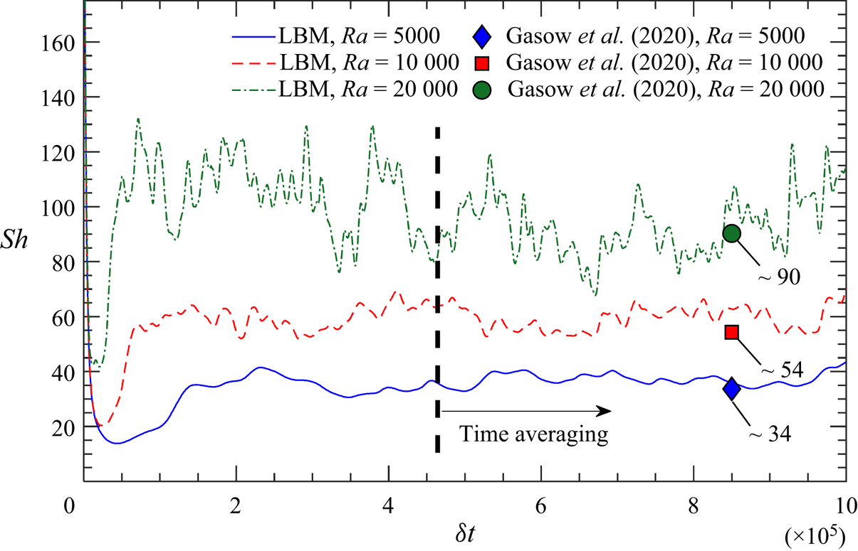
Figure 2 shows the temporal evolution of the horizontally averaged Sherwood numbers (Sh) obtained from DNS for H/m = 20 and ϕ = 0.56 (m/d = 1.5) at the Schmidt number Sc = 1. The time-averaged Sherwood numbers are Sh = 36.85, 59.01 and 92.97 for the respective cases at Ra = 5000, 10 000 and 20 000. Good agreement is demonstrated between our LBM results and those from Gasow et al. (Reference Gasow, Lin, Zhang, Kuznetsov, Avila and Jin2020). It is pointed out that in this work the time-averaging of the Sherwood number and Nusselt number was performed over a duration of 500 000δt once a statistically steady state was reached (as shown in figure 2).
Sherwood number (Sh) versus dimensionless time δt at Ra = 20 000, Sc = 1, H/m = 20 and m/d = 1.5 (ϕ = 0.56).

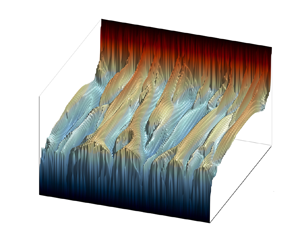
In addition, the instantaneous concentration field from the DNS at Ra = 20 000 is provided in figure 24 in Appendix A. Similarly, the macroscale DOB model implemented with the LBM is also applied for mass transfer; and a snapshot of the instantaneous concentration field for the case of Ra = 20 000 is given in figure 25 of Appendix A. Both concentration fields in figures 24 and 25 demonstrate excellent agreement in plume shape, micro-plumic behaviour near the wall and frequency of vertical plume columns with those shown in Gasow et al. (Reference Gasow, Lin, Zhang, Kuznetsov, Avila and Jin2020).
4.2. DNS and DOB modes for heat transfer
Further validation of the DNS-LBM model for heat transfer is performed by comparison with natural convection results obtained by Liu et al. (Reference Liu, Jiang, Chong and Zhu2020) for a domain ( $\varGamma$ = 1) filled with circular blocks. The referenced study differs from ours in that the side walls are insulated and non-penetrative, and circular obstacles are used instead of squares. In Liu et al. (Reference Liu, Jiang, Chong and Zhu2020), the effects of porosity in both porous and non-porous media were presented through the use of an immersed boundary method (IBM) in the Euler–Lagrange framework. It is pointed out that Liu et al. considered the Nusselt number based on the fluid thermal conductivity (Miansari et al. Reference Miansari, Gorji, Ganji and Hooman2015):
 \begin{equation}N{u_f} = \dfrac{{\displaystyle\int_w {\overline {\dfrac{{\partial \tilde{T}}}{{\partial \tilde{y}}}} \,\textrm{d}A} }}{{{A_w}}}.\end{equation}
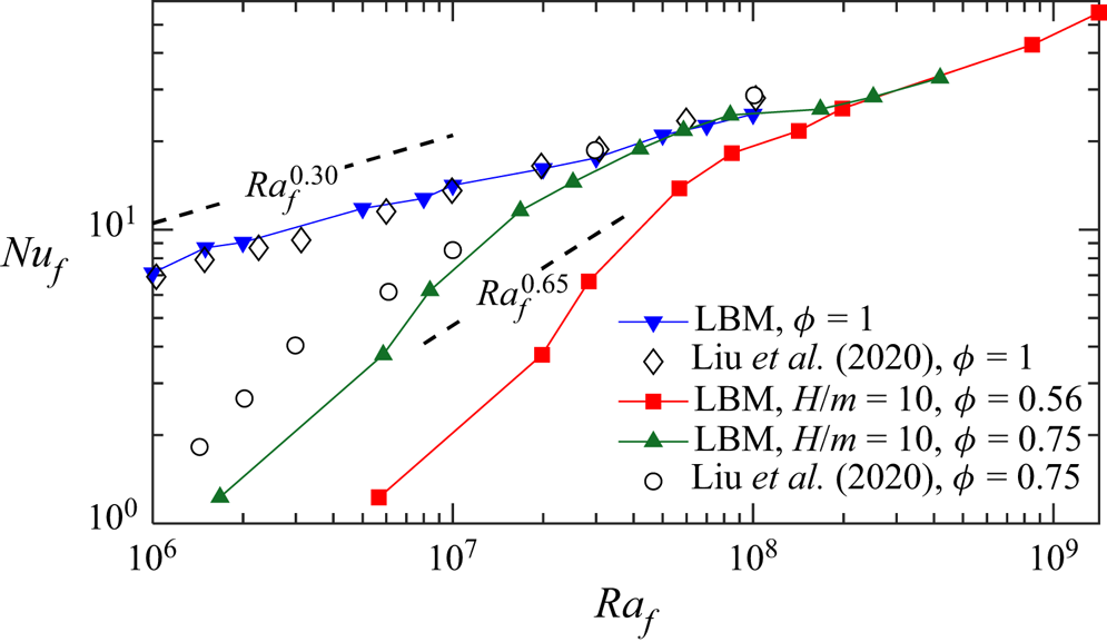
Three main points are considered for validation: (1) the Nusselt number for traditional RBC (ϕ = 1) follows an effective power law near  $N{u_f} \propto Ra_f^{0.3}$ (Niemela et al. Reference Niemela, Skrbek, Sreenivasan and Donnelly2000; Zhang et al. Reference Zhang, Yang, Zeng, Chen, Wang and Chew2017; Iyer et al. Reference Iyer, Scheel, Schumacher and Sreenivasan2020) in the range considered within this work; (2) in the lower Raf range (106~108), an increase in Nuf is expected as ϕ increases; and (3) in this lower Raf range, a steep effective power law
 $N{u_f} \propto Ra_f^{0.65}$ was found for thermal convection in porous media. It is pointed out that Liu et al. assumed thermal properties to be the same in both phases, thus the results presented here only consider σ = 1 and ks/kf = 1 for consistency.
The results are compared in figure 3. The effective power law scales and presented trends from our LBM simulations match well with the reported results for non-porous media (ϕ = 1). Furthermore, their predicted effects of porosity on Nuf are observed with LBM simulations as ϕ is varied. The difference observed at ϕ = 0.75 is attributed to the different solid-block shapes (square versus circular geometry), boundary conditions imposed on the side walls (periodic versus no-slip/insulated) and the variation in pore size. Overall, the results agree well, and a distinct transition from low-Ra Darcy-type convection to high-Ra convection is present and consistent with Liu et al. (Reference Liu, Jiang, Chong and Zhu2020).
Variations of Nuf with Raf for different ϕ with Pr = 1, σ = 1 and ks/kf = 1.

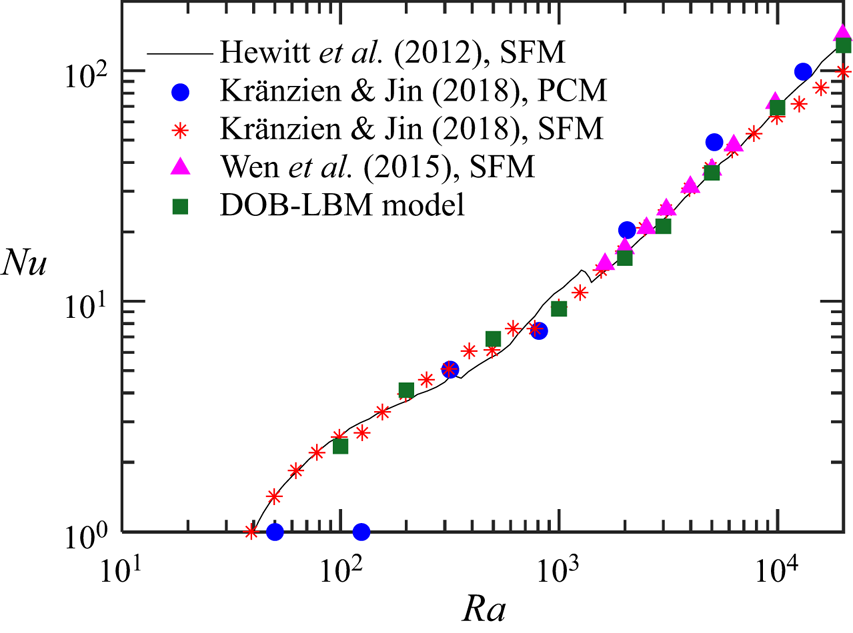
The solutions to the DOB equations for thermal convection have been studied with quite a few numerical methods: (1) Hewitt et al. (Reference Hewitt, Neufeld and Lister2012) used a SFM where (3.14) was solved with a spectral method and (2.23) with an alternating direction implicit method; (2) Kränzien and Jin (Reference Kränzien and Jin2018) solved the SFM equations with a second-order implicit backward method used for the time discretisation and a second-order central-difference scheme used for spatial discretisation; (3) Kränzien and Jin used a pressure correction method (PCM) where an intermediate velocity field was determined from the momentum equation and then a corrected pressure term was added to satisfy the continuity equation; and (4) Wen et al. (Reference Wen, Corson and Chini2015) used a Fourier–Chebyshev pseudospectral method to solve the SFM-based equations. It is noted that the parameters in these studies all used ks/kf = 1 and σ = 1. Thus, our SFM-based LBM model is also implemented with these inputs. Corresponding results are summarised in figure 4 for each of the above-mentioned methods and our DOB-LBM model. Excellent agreement is observed for the wide range of Ra studied, thus we consider the present DOB-LBM model for thermal convection validated.
Variations of Nu with Ra for the case of σ = 1 and ks/kf = 1 from DOB simulations.

5. Results and discussion
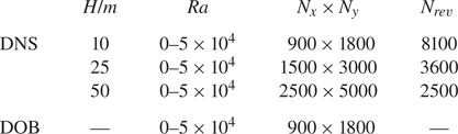
Table 1 lists the grid resolution used for both DOB and DNS simulations, where Nrev is the number of cells within each REV. A mesh independence study was performed for H/m = 25 and Ra = 5000, where the grid resolution per REV was varied among Nrev = 900, 1600, 2500, 3025 and 3600. We found that that the variation of Nu was less than 5 % for succeeding mesh sizes after Nrev = 2500, thus we consider Nrev = 2500 as our minimum mesh resolution. Furthermore, following Shishkina et al. (Reference Shishkina, Jam Stevens, Grossmann and Lohse2010) and Liu et al. (Reference Liu, Jiang, Chong and Zhu2020), for RBC the Kolmogorov length scale η can be estimated by  $\eta = HP{r^{1/2}}/{[R{a_f}(N{u_f}-1)]^{1/4}}$ and the Batchelor scale ηB by
 ${\eta _B} = \eta P{r^{ - 1/2}}$. At Ra = 50 000, for the highest value Nuf obtained within this work, the grid spacing remains below ~0.44η and ~0.44ηB. Therefore, we consider the mesh resolution sufficient. To reduce the complexity of the study we set the Prandtl number to be Pr = 1 throughout this work.
Details of grid resolutions used in simulations.

5.1. Permeability and effective thermal conductivity
To compare DNS with DOB results, the permeability, K, was determined by simulating isothermal forced convection in the porous medium. Using this approach, K is determined by the ratio of an applied pressure gradient to the mean velocity (averaged over both the fluid and solid phase). It is pointed out that the conventional Darcy number,  $D{a_C} = K/{d^2}$, is defined as the ratio of the permeability to a characteristic length of the solid phase. Thus, DaC is only dependent upon porosity while
 $Da = D{a_C}{d^2}/{H^2}$ includes a dependence on both porosity and pore size. The obtained values of DaC from the permeability study with the LBM are presented in table 2; a comparison to results in Gasow et al. (Reference Gasow, Lin, Zhang, Kuznetsov, Avila and Jin2020) is also shown demonstrating excellent matching.
Main parameters for DOB and DNS models.

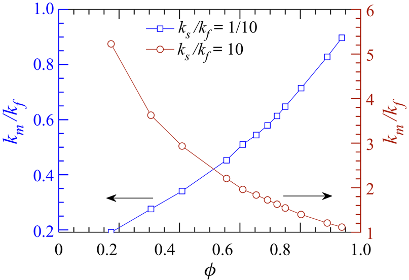
Furthermore, the stagnant effective thermal conductivity of the porous medium, km, is also obtained with the LBM model, where  ${k_m} = ({k_f}/{A_w})\int_w {\overline {\partial \tilde{T}/\partial \tilde{y}} \,\textrm{d}A}$ is determined with pure conduction (Ra = 0). It is pointed out that while only kf is explicitly present in the calculation of km because the solid blocks are not touching the upper and lower walls in the considered simulation domain (figure 1), the temperature gradient evaluated on the walls depends on both ks and kf. It is also worth mentioning that km depends on ks, kf and the structure of the porous medium and cannot always be assumed as the simple volumetric
 $({k_m} = \phi {k_f} + (1 - \phi ){k_s})$ or harmonic mean (Wang & Pan Reference Wang and Pan2008; Karani & Huber Reference Karani and Huber2017). Values of km/kf used in this work are listed in table 2. In addition, the variations of the normalised effective thermal conductivity (km/kf) at different porosities are also presented in figure 5. It should be noted that (1) for ks/kf < 1, km/kf increases as the porosity ϕ increases, whereas (2) for ks/kf > 1, km/kf decreases as ϕ increases. One should also note the similarity in the definition of km and that in the denominator of Nu for DNS simulations in (2.13). Further implications of these effects are discussed in the following sections.
Variation of the normalised effective thermal conductivity (km/kf) with porosity ϕ.

5.2. Effects of pore size
In this section, the influence of varied solid arrays on the convection dynamics are examined. For this section, we consider only the case with the same thermal transport properties in the two phases (i.e. ks/kf = 1 and σ = 1, thus γ = 1 and  $\bar{\phi } = 1$). The effects of different transport properties on thermal convection are presented in § 5.3. It is stressed that in the present study the conduction within the solid blocks is considered; this is distinct from several previous pore-scale studies of solutal convection where the solid phase is impermeable.
5.2.1. Mega and proto-plumes
Instantaneous volume-averaged temperature fields at Ra = 10 000 obtained from DOB simulations and DNS at ϕ = 0.56 are shown in figures 6 and 7, respectively. The volume-averaged temperature fields from DNS are obtained through weighted averaging over the REV as  ${\hat{T}_{rev}} = (\sum\nolimits_f {\rho {c_p}\tilde{T}} + \sum\nolimits_s {\rho {c_p}\tilde{T}} )/{(\rho {c_p})_m}$.
Instantaneous temperature field at Ra = 10 000 from DOB simulations.

Instantaneous temperature fields at Ra = 10 000 from DNS with ϕ = 0.56 for (a) H/m = 10, (b) H/m = 25 and (c) H/m = 50.

Interestingly, as the pore size is reduced (through increasing H/m), the characteristic width of the interior mega-plumes decreases whereas the spatial frequency of mega-plumes increases. This behaviour is of course absent in RBC and is uncaptured through the DOB equations. It is pointed out that a similar observation was noted by Gasow et al. (Reference Gasow, Lin, Zhang, Kuznetsov, Avila and Jin2020) in the study of mass transfer. Furthermore, the results suggest that as the pore size continues to decrease  $(H/m \to \infty )$, the DOB simulations will approach those of DNS. In the framework of the DOB equations, a major assumption is that the terms on the order of O(1/Da) dominate. For H/m = 10 with ϕ = 0.56, the Darcy number is Da = 3.53 × 10⁻⁵, whereas for H/m = 50, Da = 1.41 × 10⁻⁶. Thus, the terms including 1/Da (terms considered in DOB equations) are expected to have a contribution of 25 times more for H/m = 50 than H/m = 10 for the porosity studied here; we believe for this reason a sufficiently small Darcy number is required for DOB and DNS results to have comparable plume development.
To better explain the role of pore size in plume development, the local temperature fields within the first few REVs near the bottom boundary (y/H = 0) are plotted in figure 8. With large pore sizes (figure 8a), the flow impedance is reduced and instabilities developed near the boundary layer can interact more easily, giving rise to large structured plume columns. However, at smaller pore sizes (figure 8c), this interaction is largely limited by the solid phase, thus the instabilities at the boundary layers tend to develop into smaller and more frequent plume columns. Again, the DOB results (figure 8d) demonstrate behaviour similar to DNS at H/m = 50, thus suggesting that DNS and DOB simulations could exhibit the same frequency of mega-plumes as  $H/m \to \infty$. A similar observation was reported by Gasow et al. (Reference Gasow, Lin, Zhang, Kuznetsov, Avila and Jin2020) when studying mega-plume frequency for solutal convection, thus, it is expected that thermal convection with a highly insulating solid phase would follow this behaviour.
Instantaneous temperature fields near the lower boundary at Ra = 10 000 with ϕ = 0.56 from (a) DNS, H/m = 10, (b) DNS, H/m = 25, (c) DNS, H/m = 50 and (d) DOB simulations.

5.2.2. Flow structures
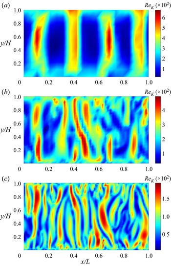
To compare the flow structures, we define a local Reynolds number following (Gasow et al. Reference Gasow, Lin, Zhang, Kuznetsov, Avila and Jin2020) based on the local velocity magnitude:
 \begin{equation}R{e_K} = \frac{{|\boldsymbol{u}|\sqrt K }}{{{\nu _f}}}.\end{equation}
It was noted by Nield and Bejan (Reference Nield and Bejan2017) that the Darcy's term dominates the drag for  $R{e_K} \ll 1$, whereas the Forchheimer's (quadratic) drag term has greater effects for ReK > 1. The Reynolds number distributions are presented in figure 9 for the three REV sizes at Ra = 10 000. The flow structures between three REV sizes are quite distinguishable, where large pores cause a low number of large structured flow paths, whereas small pore sizes cause numerous chaotic and disordered flow paths. Slightly higher Reynolds numbers are observed for lower H/m. A possible reason for this is the reduction in flow resistance (higher Darcy number at larger pore sizes), however, further study would be required to make a generalised statement of proportionality. Nonetheless, the maximum Reynolds number observed here is ~6 × 10⁻², thus we believe that the elimination of the Forchheimer's term is a valid assumption for the ranges of Ra studied.
Snapshots of the instantaneous Reynolds number ReK at Ra = 10 000 from DNS with ϕ = 0.56 for (a) H/m = 10, (b) H/m = 25 and (c) H/m = 50.

5.2.3. Nu–Ra scaling
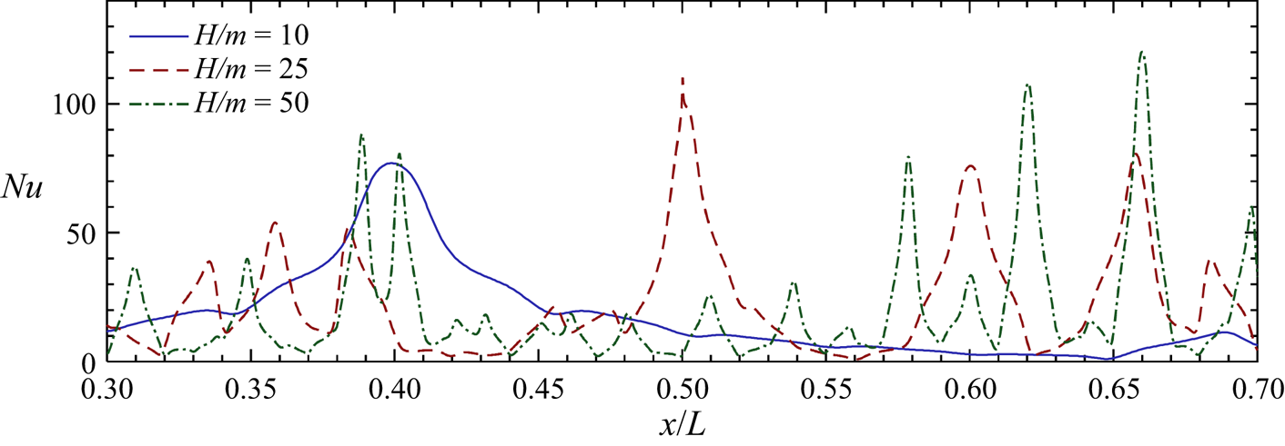
Before the discussion on the overall Nu–Ra scaling, the local Nu distributions on the walls at different pores sizes and Ra values are examined. Figure 10 shows the local Nu at the bottom boundary for the three pore sizes studied. It is pointed out that the local Nusselt numbers evaluated at the top and bottom walls should exhibit a similar magnitude and frequency of peaks; this was verified in our LBM results across a wide range of parameters, thus the local Nu values are only shown at the bottom wall. It is clear from figure 10 that at a fixed Ra the changes in frequency and magnitude of the local Nusselt number with the pore size follow the trend in plume development shown in figure 8. In addition, the local Nu values at the bottom wall from both DNS and DOB models are shown in figure 11 for varying Ra. Although both models show increased number of peaks and overall magnitude in Nu when Ra increases, the DOB results at Ra = 10 000 and 20 000 have considerably more peaks in comparison with DNS. Recalling figures 6 and 7, DOB simulations exhibit boundary layers filled with quite frequent micro-plumes (also called proto-plumes), however, these micro-plumes appear to be suppressed by the solid phase in DNS, especially at large pore sizes. Thus, a possible explanation for the high-frequency Nu peaks found in DOB results in figure 11 is the inclusion of these micro-plumes, which induce small local changes in the temperature field near and within the boundary layers.
Variation of local Nusselt number with REV size (H/m) at bottom wall for Ra = 10 000 and ϕ = 0.56.

Variation of local Nusselt number with Ra at the bottom wall with σ = 1, ks/kf = 1, and ϕ = 0.56 from (a) DNS at H/m = 25 and (b) DOB simulations.

The scaling of the overall Nusselt number for both DOB and DNS results at different pore sizes is given in figure 12. We find that the DOB results overestimate the rate of heat transfer for the range of Ra considered here. In contrast to previously computed results for mass transfer (Gasow et al. Reference Gasow, Lin, Zhang, Kuznetsov, Avila and Jin2020) with no discernible trend in the Sherwood number with pore size, the DNS results shown here suggest that the heat transfer rate increases as pore size decreases. For H/m = 10, the DNS results appear to trend towards an effective power law near  $Nu \propto R{a^{0.319}}$ (Keene & Goldstein Reference Keene and Goldstein2015) at higher Rayleigh numbers, whereas for H/m = 50 the scaling remains near
 $Nu \propto R{a^{0.9}}$. Nonetheless, we would expect
 $Nu \propto R{a^{{\sim} 0.319}}$ scaling to be reached at higher values of Ra regardless of pore size once the length scales of flow become smaller than the pore scale (Hewitt Reference Hewitt2020; Liu et al. Reference Liu, Jiang, Chong and Zhu2020).
Comparison of Nu–Ra relations between DOB and DNS results with different pore sizes and a fixed porosity ϕ = 0.56.

5.2.4. Temperature and velocity statistics
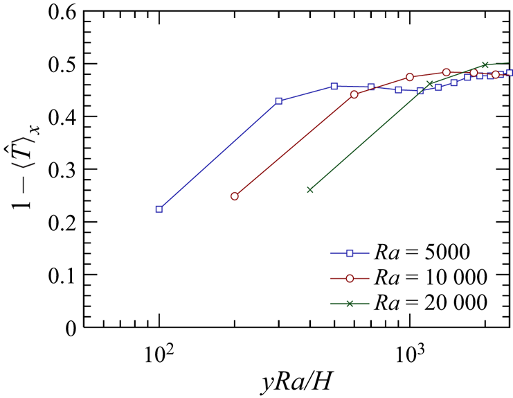
First, figure 13 shows the vertical profiles of the temporally and horizontally averaged temperature [both scalars and their root mean squares (r.m.s.)] and r.m.s. of x- and y-direction velocity components from DOB simulations. It has been suggested (Huppert & Neufeld Reference Huppert and Neufeld2014; Kränzien & Jin Reference Kränzien and Jin2018) that the boundary layer thickness is determined by 1/Ra. Thus, we normalise the dimensionless coordinate in figure 13 as yRa/H, upon which the temperature and velocity profiles at different Ra become almost identical. This is consistent with the study of pore size effects in mass transfer by Gasow et al. (Reference Gasow, Lin, Zhang, Kuznetsov, Avila and Jin2020).
DOB results: (a) vertical profiles of temporally and horizontally averaged temperature, and root mean squares of (b) temperature fluctuation, (c) ux fluctuation and (d) uy fluctuation.

In contrast, normalising the DNS results at H/m = 25 by yRa/H shows quite different profiles, as shown in figure 14. Gasow et al. suggested that for solutal convection the statistics of the concentration and velocity fields are not only influenced by Ra, but also by the pore size (m/H). We find it instrumental to test the consistency of this observation for thermal convection. Therefore, temporally and horizontally averaged temperature and r.m.s. of the temperature and velocity fields at different Rayleigh numbers from DNS are shown in figure 15. We find that the lines collapse when the dimensionless coordinate y/H is scaled by the pore size, suggesting that the pore-scale effects play a major role in shaping the boundary layer and flow structure in both thermal and solutal convection. Recent studies have begun to investigate these pore-scale factors for solutal convection through modified/extended DOB equations. Wen, Chang, and Hesse (Reference Wen, Chang and Hesse2018) investigated the effects of mechanical dispersion through the use of a Fickian dispersion tensor, introducing two additional dimensionless parameters: the dispersive Rayleigh number Rad = H/εt and the dispersivity ratio r = εl/εt where εt and εl are the transverse and longitudinal dispersivities, respectively. Their work showed that increasing the mechanical dispersion would increase the plume spacing, thus showing that the grain/pore size plays a role in shaping the plumes and flow pattern. A recent work by Gasow et al. (Reference Gasow, Kuznetsov, Avila and Jin2021) included the effects of momentum dispersion through a ‘two-length-scale diffusion’ model. By considering the pore-scale momentum transport through an effective diffusion term, they were able to obtain more accurate Sherwood numbers than with the traditional DOB equations. Nonetheless, there is still a need to extend and build upon those works for thermal convection where additional phenomena are involved.
Vertical profiles of temporally and horizontally averaged temperature from DNS at H/m = 25.

DNS results at H/m = 25: (a) vertical profiles of temporally and horizontally averaged temperature, and root mean squares of (b) temperature fluctuation, (c) ux fluctuation, and (d) uy fluctuation.

5.3. Effects of conjugate heat transfer
Now we consider the effects of conjugate heat transfer on thermal convection when the fluid and solid phases have different transport properties (e.g. ks/kf ≠ 1 and/or σ ≠ 1). We begin by emphasising that ks/kf and σ are independent parameters with ks/kf representing the thermal conductivity ratio and σ the heat capacity ratio, whereas the thermal diffusivity ratio is related to those two through γ = (ks/kf)/σ. To explore the respective effects of both, two groups of cases are examined: (1) group 1 with varying ks/kf at σ = 1, and (2) group 2 with varying σ at ks/kf = 1.
5.3.1. Nu–Ra relations
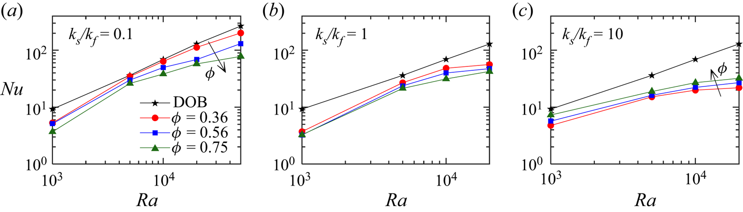
Figure 16 shows the Nu–Ra relations for various ks/kf (group 1) and ϕ values from both DNS and DOB results. Instantaneous snapshots of the temperature fields at Ra = 20 000 and ϕ = 0.56 can be found in Appendix B. As the effect of thermal conductivity enters the DOB equations through only Ra and  $\bar{\phi } = 1$ when σ = 1 (see (2.17a–c)), a single line is shown for DOB simulations. The DNS results show that both ks/kf and porosity ϕ have a significant effect on Nu. A few key observations are noted: (1) at fixed ϕ and Ra, the magnitude of Nu appears to decrease as ks/kf increases, (2) for ks/kf < 1, Nu decreases as ϕ increases; however, for ks/kf > 1, Nu increases with ϕ, and (3) DOB simulations appear to overpredict the heat transfer rate regardless of ks/kf and ϕ, with larger discrepancy observed for higher ks/kf and Ra. The effects in points (1) and (2) can be attributed to the physical differences at the pore scale for a fixed Ra. For example, at Ra = 20 000 and ϕ = 0.56 the unconfined Rayleigh number at ks/kf = 0.1 is Raf = 1.60 × 10⁹, whereas for ks/kf = 10 the number is Raf = 8.41 × 10⁹. Thus, at fixed Ra, ϕ and H/m, Raf will be greater for larger ks/kf. Furthermore, a larger ks/kf is also representative of a more conductive solid phase and varying porosities indicate differences in permeability (higher ϕ yield smaller Raf values with fixed Ra, ks/kf, and H/m). The major conjecture of the DOB equations is that regardless of ks/kf and ϕ, the ratio of the overall to conductive heat transfer rate (i.e. the Nusselt number) is constant across a REV at a fixed Ra. Our DNS results show that this is not true, suggesting that effects of ks/kf and ϕ should be considered independently of Ra.
Comparison of Nu–Ra relations at different porosities for Group 1 cases (σ = 1): (a) ks/kf = 0.1, (b) ks/kf = 1 and (c) ks/kf = 10. The reference DOB result is independent of both ϕ and ks/kf, and H/m = 25 for all DNS results.

As mentioned previously, comparisons of Nu–Ra scaling in literature are widespread. Namely, theoretical studies based on the DOB equations have predicted ultimate regime scaling exponents in ranges of 0.9–0.95, whereas pore-scale and experimental studies have found values closer to 0.29–0.33. In addition, the Nu values obtained based on experiments varied largely, raising questions on what parameters (ϕ, H/m, ks/kf, etc.) are the main contributors. Previous discussion has shown that both the pore size and ks/kf affect the Nu–Ra scaling. Thus, we find it valuable to compare selected DNS at varying ks/kf and σ to reported experiments (Kladias & Prasad Reference Kladias and Prasad1991; Keene & Goldstein Reference Keene and Goldstein2015) as shown in figure 17. The characteristic pore size, H/Lpore (Lpore is the pore-scale solid block diameter or width), in experiments ranged from 3.048 to 12.7; whereas ks/kf varied from approximately 0.33 to around 321. Overall, the DNS results in the limits of ks/kf and σ appear to span the range of experimental data reasonably well. The DNS results also capture the nonlinear Nu–Ra scaling observed in experiments (Keene & Goldstein Reference Keene and Goldstein2015).
Comparison of Nu–Ra relations between reported experiments and present DNS at H/m = 10 and ϕ = 0.56 (m/d = 1.5).

Next, we focus on the effects of the heat capacity ratio σ. Figure 18 presents the Nu–Ra relations for σ = 0.1, 1, and 10 with ks/kf = 1 fixed (Group 2) from both DOB and DNS results. In contrast to the effect of ks/kf, the effects of σ enter the DOB equations through both Ra and  $\bar{\phi }$ ((2.17a–c)). In the DOB equations, at a fixed Ra,
 $\bar{\phi }$ is manifested through the convective term
 $\hat{\boldsymbol{\nabla } }\boldsymbol{\cdot }(\hat{\boldsymbol{u}}\hat{T}/\bar{\phi })$ in (2.23). Thus, one would expect the convective strength to follow
 $1/\bar{\phi }$. This is observed in figure 18(a)–18(c), where Nu decreases as ϕ increases for σ < 1 (because
 $\bar{\phi } = 0.1 + 0.9\phi$ at σ = 0.1), whereas Nu increases as ϕ increases for σ > 1 (since
 $\bar{\phi } = 10 - 9\phi$ at σ = 10).
Comparison of Nu–Ra relations at different porosities for Group 2 cases (ks/kf = 1): (a) σ = 0.1, (b) σ = 1 and (c) σ = 10 are from DOB results, and (d) σ = 0.1, (e) σ = 1 and (f) σ = 10 are from DNS results at H/m = 25.

Interestingly, the same trend in the variations of Nu with σ and ϕ is observed in the DNS results in figure 18(d)–18(f), suggesting that the effects of varying σ alter the convection strength in a similar manner in both DOB and DNS results. In the DNS equations, the effects of varying σ at a fixed Ra are manifested through scaling of Raf (also by  $1/\bar{\phi }$). Thus, σ plays a similar role in determining the Nusselt number for both DOB and DNS results. In addition, the instantaneous snapshots of the temperature fields for varying σ values from both DOB and DNS results are provided in Appendix B. Both DOB and DNS temperature fields appear to exhibit distinct mega-plume frequency and size, with σ = 0.1 showing more frequent and smaller plumes, and the opposite for σ = 10. This suggests that the peak wavenumber follows
 $Ra/\bar{\phi }$ for the range of parameters studied here. It should be noted that previous studies have shown that the peak wavenumber is dependent upon the initial fields, aspect ratio of the convection cell and pore size (Hewitt et al. Reference Hewitt, Neufeld and Lister2012; Gasow et al. Reference Gasow, Lin, Zhang, Kuznetsov, Avila and Jin2020) and are not unique for Ra > 39 716 (Wen et al. Reference Wen, Corson and Chini2015), thus, more detailed investigations are needed to fully characterise the peak wavenumber. This is out of the scope of the present work.
5.3.2. Thermal boundary layer analysis
In this section, we investigate the characteristics of the thermal boundary layers from both DOB and DNS results. As discussed in § 5.2.4, several works based on the DOB equations have suggested that the boundary layer thickness is determined by 1/Ra (Huppert & Neufeld Reference Huppert and Neufeld2014; Kränzien & Jin Reference Kränzien and Jin2018; Gasow et al. Reference Gasow, Lin, Zhang, Kuznetsov, Avila and Jin2020), however, these have been limited to cases where σ = 1. The temporally and horizontally averaged temperature profiles from DOB simulations are first plotted in figure 19 when the dimensionless coordinate y/H is scaled by 1/Ra following that in figure 13(a). It is obvious that in addition to Ra, both ϕ and σ have significant effects on the boundary layer thickness. As the convective term in the DOB equations is scaled by the effective volumetric heat capacity ratio  $\bar{\phi }$, we hypothesise that the boundary layer thickness for thermal convection between the two phases with different transport properties be determined by both Ra and
 $\bar{\phi }$ in the DOB model, and the results are shown in figure 20, where it can be observed that all the temperature profiles effectively collapse to a narrow band, confirming our hypothesis that the thermal boundary layer thickness is determined by
 $\bar{\phi }/Ra$.
Temporally and horizontally averaged temperature profiles from DOB simulations when y/H is scaled by 1/Ra.

Temporally and horizontally averaged temperature profiles from DOB simulations when y/H is scaled by  $\bar{\phi }/Ra$.

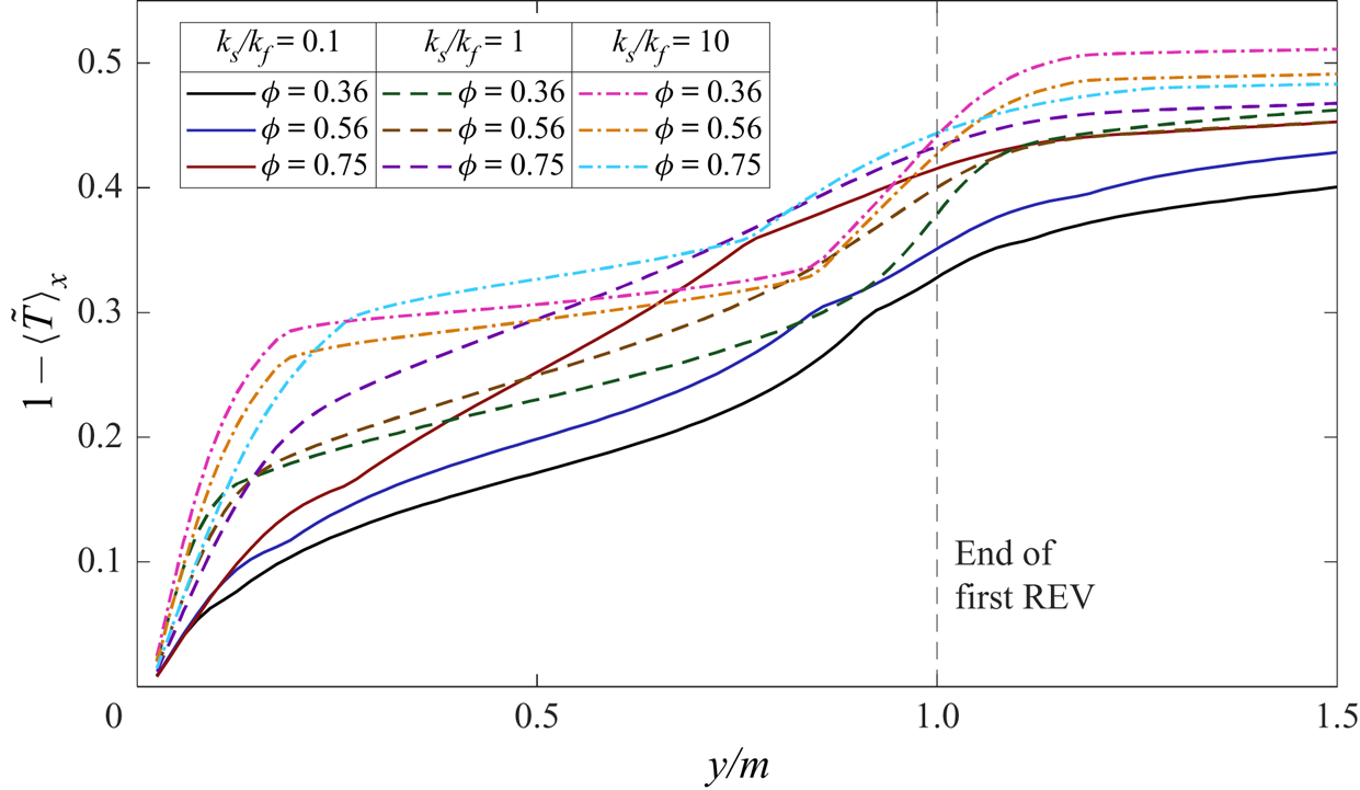
As discussed in § 5.2.4, the thermal boundary layer thickness from DNS results at ks/kf = σ = 1 is determined by the pore scale (m/H), consistent with the scaling presented in Gasow et al. (Reference Gasow, Lin, Zhang, Kuznetsov, Avila and Jin2020) for mass transfer. It is of interest to examine this for ks/kf ≠ 1 and/or σ ≠ 1. Figure 21 shows results for varying ks/kf with σ = 1 (group 1) when y/H is rescaled by the pore scale (m/H). Surprisingly, the profiles appear to overlap reasonably well regardless of ks/kf and Ra, suggesting that the pore size is also the controlling factor for thermal convection with varying conductivities in the two phases.
Temporally and horizontally averaged temperature profiles from DNS for Group 1 cases with varying ks/kf values when y/H is scaled by m/H.

We also find it instructive to show in detail the local boundary layers within the first REV. Figure 22 shows the temperature profiles for Ra = 10 000 and H/m = 25 near the lower wall. Although the complete boundary layer is determined by the pore size, the local behaviour near the boundary is heavily influenced by variations in thermal properties. Near the wall, the boundary layer is encompassed in only the fluid phase, thus we would expect a larger temperature gradient at higher Raf (higher ks/kf), as noticed in figure 22. Furthermore, the central region of the first REV contains the solid phase. As expected, the temperature gradient in this region is smaller for ks/kf = 10, and vice versa for ks/kf = 0.1. This local behaviour is altogether uncaptured by the DOB equations, which negate the effects of local temperature and velocity fluctuations captured through thermal dispersion,  ${(\rho {c_p})_f}\boldsymbol{\nabla }\boldsymbol{\cdot }(\phi {\langle \boldsymbol{\mathord{\buildrel{\lower3pt\hbox{$\scriptscriptstyle\smile$}} \over u} }\mathord{\buildrel{\lower3pt\hbox{$\scriptscriptstyle\smile$}} \over T} \rangle ^f})$. The results shown here suggest that future work aimed at improving macroscopic models for thermal convection should consider these local effects.
Local temperature profiles from DNS for σ = 1, Ra = 10 000 and H/m = 25.

Furthermore, figure 23 shows the results for the varying σ cases with ks/kf = 1 (group 2) when y/H is rescaled by the pore size m/H. Similar to group 1 cases, all profiles at σ = 0.1 and 1 collapse well. However, for low Ra (~5000) and σ = 10, the boundary layers are thicker and are not limited to only the first few REVs, this is again due to the much lower unconfined Rayleigh number Raf for those cases. Recalling that Raf is related to Ra as  $R{a_f} = Ra({k_m}/{k_f})/Da[\phi + (1 - \phi )\sigma ]$, larger σ values indicate smaller Raf, for which the convection will be less significant and conduction can become dominant (e.g. when
 $\sigma \to \infty$,
 $R{a_f} \to 0$ and pure conduction is attained). The profiles at Ra = 5000 and σ = 10 demonstrate the onset of this behaviour. Overall, the present boundary layer analysis between the DOB and DNS results clearly demonstrates the distinct local behaviours that would contribute to the different thermal convection characteristics in porous media when formulated through the DNS and the volume-averaged DOB equations with additional assumptions.
Temporally and horizontally averaged temperature profiles from DNS for Group 2 cases with varying σ values when y/H is scaled by m/H.

6. Conclusions
We performed high-resolution DNS of thermal convection in a simplified 2-D porous structure and compared results with volume-averaged formulations based on the DOB equations. Both DNS and DOB simulations were realised with the LBM, with a novel method of solving the SFM equations with the LBM being proposed and validated. Comparisons of DNS and DOB results demonstrated that both the pore size and conjugate heat transfer play large roles in shaping the structure of the thermal and flow fields and in determining the Nusselt number.
Upon comparing different pore sizes from DNS, it was found that larger pores (higher Darcy number) created less frequent but structured plumes, and the opposite for smaller pores. Between DNS and DOB results, the temperature fields matched quite well for small pores with H/m = 50. A possible explanation for this is that the terms considered in the DOB equation (on the order of 1/Da) dominate in the interior regime, while the boundary layer is governed instead by the pore size within the first few REVs. The flow structure was compared for all REV sizes at Ra = 10 000. Results showed that the local Reynolds number increased with pore size, however, it is stressed that a detailed analysis of the effects of porosity and the Rayleigh number would be required to make a generalised statement and is considered out of the scope of this paper. We believe the elimination of the Forchheimer term in the DOB equations is valid for the range of Ra studied, as evidenced by the low magnitudes of ReK (near 7 × 10⁻² at Ra = 10 000).
On the effects of conjugate heat transfer, we studied two groups of cases: group 1 with varying ks/kf at σ = 1 and group 2 with varying σ at ks/kf = 1. When comparing the Nusselt numbers for different ks/kf and ϕ at fixed Ra (group 1), we observed that the DNS results predict a decrease in Nu with increasing ϕ when ks/kf < 1, and the opposite for ks/kf > 1. This behaviour was altogether uncaptured by the DOB equations that only account for the conductivity ratio through Ra. For varying σ (group 2), a similar trend was observed in both DOB and DNS results, i.e. Nu decreases as ϕ increases for σ < 1, and the opposite for σ > 1. This is attributed to the scaling of the convective term in the DOB equations and scaling of Raf in the DNS equations. Furthermore, a comparison of Nu = f(Ra) scaling with selected experiments of thermal convection was shown. DNS results demonstrated large variations in Nu for different ks/kf and σ and appeared to approach power law scaling near  $Nu \propto R{a^{{\sim} 0.319}}$ at high Ra. In comparison, the DOB model maintains scaling of
 $Nu \propto R{a^{0.9}}$. The variations in pore size and thermal conductivity ratio observed in DNS help to explain the large scatter of Nu = f(Ra) data in the literature for thermal convection.
A detailed analysis of the temporally and horizontally averaged temperature profiles was also performed for both DOB and DNS results. Following previous works based on the DOB equations that suggest 1/Ra scaling, a unified extended scaling was proposed as  $\bar{\phi }/Ra$ to account for the effects of different transport properties. When the dimensionless coordinate y/H is rescaled by
 $\bar{\phi }/Ra$, the temperature profiles in the boundary layer were shown to collapse for a wide range of inputs (Ra = 1000 to 20 000 at different ϕ and σ values). Furthermore, the boundary layer thickness from DNS results is determined by the pore size (m/H) for general cases, which is consistent with recent works on mass convection (Gasow et al. Reference Gasow, Lin, Zhang, Kuznetsov, Avila and Jin2020, Reference Gasow, Kuznetsov, Avila and Jin2021). For the special cases at low Ra and high σ in group 2, the boundary layers were thicker due to the decrease in convection strength (Raf is considerably smaller for these cases).
Overall, our results presented herein show that conjugate heat transfer and pore-scale parameters play essential roles in the dynamics of thermal convection. Although the DOB equations are useful for situations where it is impractical to obtain/simulate the porous domain, care should be taken to verify that Lpore/H is sufficiently small for the volume-averaging to be applied and that the thermal properties are reasonably close. Furthermore, our results along with previously reported observations of mass transfer allow for possible improvement of the DOB models, where underlying physics including pore-scale parameters and boundary layer behaviour can be included through the addition of momentum dispersion, thermal dispersion, and viscous diffusion terms.
Supplementary movies
Supplementary movies are available at https://doi.org/10.1017/jfm.2022.491.
Acknowledgements
The authors thank the three anonymous reviewers for their valuable comments that helped improve this paper.
Funding
The authors gratefully acknowledge the support of the National Science Foundation, United States (NSF award number OIA 2031701). The computer simulations used the NSF Extreme Science and Engineering Discovery Environment (XSEDE) under award allocation number TG-DMR190112 and the clusters in the High Performance Computing Collaboratory (HPC2) at Mississippi State University.
Declaration of interests
The authors report no conflict of interest.
Appendix A. Model validation to solutal convection
In this Appendix, we provide additional comparisons and details used for model validation. Following the discussion in § 4.1, instantaneous contours of the concentration field at Ra = 20 000, H/m = 20 and m/d = 1.5 from the DNS and DOB models are given in figures 24 and 25, respectively. The shape of the mega-plumes and micro-plumic development near the boundary layers are quantitively compared to figures 4(b) and 4(c) in (Gasow et al. Reference Gasow, Lin, Zhang, Kuznetsov, Avila and Jin2020), demonstrating good agreement.
DNS based instantaneous concentration field for Ra = 20 000, H/m = 20 and m/d = 1.5 (comparable to figure 4(b) in Gasow et al. Reference Gasow, Lin, Zhang, Kuznetsov, Avila and Jin2020).

DOB-based instantaneous concentration field for Ra = 20 000 (comparable to figure 4(c) in Gasow et al. Reference Gasow, Lin, Zhang, Kuznetsov, Avila and Jin2020).

Appendix B. Additional temperature contours for Ra = 20 000 from DNS and DOB models
Following the discussion in § 5.3.1, instantaneous temperature contours from the DOB model at Ra = 20 000 and ϕ = 0.56 with varying σ are provided in figure 26. A clear distinction in the size and frequency of the mega-plumes is present. Figure 27 gives the instantaneous temperature contours from DNS at Ra = 20 000, k s/k f = σ = 1, ϕ = 0.56 and H/m = 25, whereas figures 28 and 29 give the corresponding results at varying k s/k f cases with σ = 1 (group 1) and varying σ with k s/k f = 1 (group 2), respectively.
Instantaneous temperature fields at Ra = 20 000 and (a) σ = 0.1, (b) σ = 1 and (c) σ = 10 from DOB simulations.

Instantaneous temperature fields at Ra = 20 000, ks/kf = σ = 1, ϕ = 0.56 and H/m = 25 from DNS.

Instantaneous temperature fields at Ra = 20 000, σ = 1, ϕ = 0.56, H/m = 25 and (a) ks/kf = 0.1 and (b) ks/kf = 10 from DNS.

Instantaneous temperature fields at Ra = 20 000, ks/kf = 1, ϕ = 0.56, H/m = 25 and (a) σ = 0.1 and (b) σ = 10 from DNS.