





1. Introduction
Oceanic turbulent mixing plays a crucial role in controlling the meridional overturning circulation and heat budget, and subsequently in shaping global climate states (Ganachaud & Wunsch Reference Ganachaud and Wunsch2000; Wunsch & Ferrari Reference Wunsch and Ferrari2004; Hieronymus et al. Reference Hieronymus, Nycander, Nilsson, Döös and Hallberg2019). Numerous efforts have been made to comprehend the connections between large-scale processes and small-scale turbulence in oceans. Compared with the stratified atmosphere, where atmospheric turbulence has been studied through spectral and structure–function analyses for decades (Gage Reference Gage1985; Frehlich & Sharman Reference Frehlich and Sharman2010), in the ocean, more attention has been focused on mesoscale and submesoscale turbulence and internal wave mixing (e.g. Meredith & Garabato (Reference Meredith and Garabato2021) and references therein), while less attention has been paid to small-scale turbulence, especially to the cascade scaling behaviours in various turbulent regimes.
The ocean is generally considered to be a stratified fluid. In stably stratified fluids, Bolgiano (Reference Bolgiano1959) and Obukhov (Reference Obukhov1959) (BO) proposed the ‘buoyant subrange’ in the spectrum, where turbulence energy is suppressed by negative buoyancy forces associated with a hydrostatically stable environment and the buoyant flux exceeds the kinetic energy flux. Based on dimensional analysis, the kinetic energy spectrum  $E_u(k)$ and the thermal energy spectrum
 $E_\theta (k)$ were predicted to scale as
 $k^{-11/5}$ and
 $k^{-7/5}$, respectively, where
 $k$ is the wavenumber. However, this BO scaling has rarely been observed in the ocean. Instead, observations of vertical wavenumber spectra of temperature in the open ocean (Gregg Reference Gregg1977; van Haren & Gostiaux Reference van Haren and Gostiaux2009) and composite spectrum of velocity shear (Gargett et al. Reference Gargett, Hendricks, Sanford, Osborn and Williams1981) showed the spectrum to fall as
 $k^{-3}$, consistent with the theoretical prediction by Monin (Reference Monin1962) and Lumley (Reference Lumley1964). More observations have found transition of the energy spectrum from
 $k^{-3}$ to
 $k^{-5/3}$, representing the scaling law in homogeneous isotropic turbulence (Kolmogorov Reference Kolmogorov1941), for high-Reynolds-number turbulence in the interior ocean (Ewart Reference Ewart1976; Gargett, Osborn & Nasmyth Reference Gargett, Osborn and Nasmyth1984; Holbrook & Fer Reference Holbrook and Fer2005; Klymak & Moum Reference Klymak and Moum2007).
Comparatively, the BO scaling has been observed in the stably stratified atmospheric surface layer (Chiba Reference Chiba1989), lower stratosphere (Cot & Barat Reference Cot and Barat1989), troposphere (Lazarev et al. Reference Lazarev, Schertzer, Lovejoy and Chigirinskaya1994), lower stratosphere and upper troposphere (Werne & Fritts Reference Werne and Fritts2000; Wroblewski et al. Reference Wroblewski, Cote, Hacker and Dobosy2010). However, different results have also been obtained in other works. The BO scaling has not been observed in weak or strong stratification at a height of 2 m over flat grassland (Okamoto & Webb Reference Okamoto and Webb1970). Turbulent wind spectra have scalings from  $11/5$ to
 $3$ for stable stratification and are closer to the Kolmogorov theory for neutral stratification at the surface atmosphere layer (Myrup Reference Myrup1969). The change from the BO to Kolmogorov scalings can be observed for different scale ranges in temperature measurements at altitudes of approximately 10 km (Wroblewski et al. Reference Wroblewski, Cote, Hacker and Dobosy2007). Although the BO scaling has also been observed in unstably stratified convective turbulence in laboratory experiments (Wu et al. Reference Wu, Kadanoff, Libchaber and Sano1990; Zhou & Xia Reference Zhou and Xia2001) and theoretical arguments (Yakhot Reference Yakhot1992; Ching Reference Ching2014), its existence is still debatable (for a review, see Lohse & Xia (Reference Lohse and Xia2010)).
Some numerical simulations report inconsistent views regarding stably stratified and convective turbulence as well. In certain simulations, the velocity spectrum follows the BO scaling in strongly stratified or moderately stratified regimes, while it follows the Kolmogorov scaling for weak stratification (Kumar, Chatterjee & Verma Reference Kumar, Chatterjee and Verma2014; Alexakis & Biferale Reference Alexakis and Biferale2018; Alam, Guha & Verma Reference Alam, Guha and Verma2019; Basu & Bhattacharjee Reference Basu and Bhattacharjee2019; Agrawal & Chandy Reference Agrawal and Chandy2021). For very weak and/or strong stratifications, where the buoyancy forces are relatively irrelevant or the flow fields are effectively two-dimensionalized, the kinetic energy spectra show the Kolmogorov scaling (Basu & Bhattacharjee Reference Basu and Bhattacharjee2019; Agrawal & Chandy Reference Agrawal and Chandy2021). In a cascade model simulation, Shestakov, Stepanov & Frick (Reference Shestakov, Stepanov and Frick2017) believe that the BO regime exists only when the work of the buoyancy force and the nonlinear energy transfer over the spectrum are balanced within a certain range of scales, which is not satisfied either in convective turbulence or in turbulence with stable stratification.
According to the literature review mentioned above, it appears that the BO scaling may exist in stratified fluids and potentially in convective turbulence, which motivates further exploration of this issue in highly turbulent oceanic environments. In addition, recent in situ observations have revealed BO-like scaling in the deep ocean (near bottom) of the Rockall Canyon (van Haren et al. Reference van Haren, Voet, Alford, Fernández-Castro, Naveira Garabato, Wynne-Cattanach, Mercier and Messias2024), the Gulf of Mexico (Polzin et al. Reference Polzin, Wang, Wang, Thwaites and Williams2021) and other regions (e.g. van Haren & Dijkstra Reference van Haren and Dijkstra2021; van Haren & Bosveld Reference van Haren and Bosveld2022). These studies suggest that the  $-7/5$ scaling in the temperature spectrum is indicative of buoyancy-driven convective turbulence (van Haren et al. Reference van Haren, Voet, Alford, Fernández-Castro, Naveira Garabato, Wynne-Cattanach, Mercier and Messias2024), which needs further clarification due to its importance in abyssal ocean exploration. The South China Sea (SCS), known as the most active marginal sea, exhibits significantly enhanced mixing with turbulence levels two orders of magnitude higher than those in the Pacific Ocean (Tian, Yang & Zhao Reference Tian, Yang and Zhao2009; Yang et al. Reference Yang, Zhao, Liang and Tian2016). The intense mixing in the SCS is primarily driven by internal waves, which originate in the Luzon Strait and propagate westward into the continental shelf and deep basin (Zhao Reference Zhao2014; Alford et al. Reference Alford2015). The Dongsha Plateau, situated on the northern continental shelf of the SCS, lies directly in the path of these internal waves, where a potential maximum balance between wave energy and instability may exist (St. Laurent et al. Reference St. Laurent, Simmons, Tang and Wang2011). Recent observations have indicated the alternative occurrence of stratified turbulence and convective turbulence in the bottom ocean of the Dongsha Plateau (Qu et al. Reference Qu2021). This unique environment provides an ideal opportunity to explore the turbulent energy cascading in different flow and stratification regimes within the ocean.
In this study, we examine the existence of BO scaling in the bottom ocean near Dongsha Atoll at a depth of 278 m on the continental shelf. The paper is organized as follows. In § 2, we present the hydrographic data and data processing. Then we describe the water characteristics and temperature spectrum scalings in § 3, discuss the BO-like scaling in the convective turbulence and stratified turbulence of different stratifications in § 4 and summarize the main points in § 5.
2. Hydrographic data and data processing
2.1. Hydrographic data
Between 15 April and 21 May 2020, a comprehensive oceanographic survey was undertaken in the SCS using the Jiageng R/V. As part of this survey, a 46-hour experiment was carried out starting at 17:44 local time (LT) on 15 May at a site northwest of Dongsha Atoll ( $21.24^{\circ }$ N,
 $116.07^{\circ }$ E) with a water depth of 278 m (figure 1a). The topographic slope angle at this location is
 $0.61^{\circ }$ based on the GEBCO topography dataset. In the experiment, an instrumented full-depth mooring was deployed, equipped with a tripod lander frame at the bottom (figure 1b). The mooring set-up included various sensors and instruments: 25 SBE56 temperature loggers (Sea-bird Electronics), 76 ONT18S temperature loggers (Ocean Net Technology Co. Ltd), three Infinity-CT (JFE Advantech), one CTD and two RBR-TD (RBR), one current meter (SeaGuard) and one ADCP (300 kHz, Teledyne RDI). The tripod lander frame had a height of 2.2 m. On one vertical arm of the frame, 22 ONT18S temperature loggers were mounted with equal spacing of 0.1 m from the lowest one, which was located 0.01 m above the bottom (
 $Dab=0.01$ m). The RBR-CTD was mounted on a different arm at
 $Dab=1.20$ m. Moving upward from the top of the frame to the sea surface, the temperature loggers were arranged as follows: 10 ONT18S temperature loggers with a vertical spacing of 1 m, 36 ONT18S temperature loggers with a spacing of 2 m,
 $20$ SBE56 temperature loggers with a spacing of 5 m and five SBE56 temperature loggers with a spacing of 20 m. Two RBR-TD sensors were mounted at
 $Dab=125.6$ and 266 m and three Infinity-CT were mounted at
 $Dab=22$,
 $55$ and 125 m. The ONT18S temperature logger was used for its small time constant of 0.3 s and a low noise level of
 $1\times 10^{-4}$
 $^{\circ }$C. It was set to sample at a rate of 16 Hz to capture the small-scale water structures. The sampling rates for RBR-CTD, RBR-TD, SBE56 and Infinity-CT sensors were set at
 $16$,
 $2$,
 $1$ and 1/60 Hz, respectively. Additionally, a down-looking 300 kHz ADCP was mounted at a depth of approximately
 $Dab=126$ m. It was programmed to sample at an interval of 60 s with a bin size of 4 m. In the present study, the focus was on the turbulent cascading behaviours within the bottom 80 m, in which the temperature was precisely recorded using
 $51$ ONT18S temperature loggers.
(a) Bathymetric map of the northeastern SCS extrapolated from GEBCO gridded bathymetry data. The tripod mooring location is represented by the red star. The coordinates ( $x,y$) are defined as
 $x$ along the slope direction (positive to the northeast) and
 $y$ in the cross-slope direction (positive onshore). The inset shows a zoomed-in view of the map near the mooring station. The grey circles indicate the CTD stations. (b) Schematic diagram illustrating the configuration of the tripod mooring.

Meanwhile, a CTD rosette cast was performed every 3 h at the mooring site, reaching a maximum depth of around 258 m, approximately 20 m above the ocean bottom. The rosette included a 300 kHz lowered acoustic Doppler current profiler (LADCP; Teledyne RDI) and an SBE911 Plus CTD to measure the flow and water properties such as velocity, temperature, salinity and pressure. The CTD collected data at a sampling rate of 24 Hz. The LADCP was configured with  $20$ bins of bin size 8 m to capture the flow characteristics. Due to the influence of wind and surface ocean currents, the vessel experienced frequent drift, but it was restored to the set location within a range of approximately 2.5 km, as shown in the inset of figure 1(a). Additionally, a vertical microstructure profiler (VMP250, Rockland Scientific) was deployed every hour from 19:00 LT on 15 May to 00:30 LT on 18 May with a sampling rate of 512 Hz, measuring the turbulent kinetic energy dissipation rate
 $\varepsilon$. To avoid potential damage from the complex topography, the VMP250 approached depths ranging from
 $5$ to 50 m above the seafloor during each deployment.
2.2. Data processing
In order to precisely measure the fine thermal variations in the bottom ocean, the ONT18S temperature loggers underwent laboratory calibration prior to field deployment. Additionally, the ONS18S temperature loggers were cross-calibrated using the data of RBR-CTD at  $Dab=1.2$ m. As a result, these calibration procedures improved the temperature loggers’ precision of
 $1\times 10^{-3}$ and resolution of
 $1\times 10^{-4}$
 $^\circ$C.
For further analysis, it is necessary to convert the in situ temperature  $T$ to potential temperature
 $\theta$ and potential density
 $\sigma _0$. This conversion relies on the relationship obtained from the full-depth temperature and salinity profiles with the SBE911 Plus CTD. As shown in figure 2(a), the potential temperature,
 $\theta$, appears to be proportional to the in situ temperature
 $T$. Figure 2(b) shows that the potential density,
 $\sigma _0$, decreases as the in situ temperature,
 $T$, increases, but the relationship is nonlinear. The best-fit equations are given by
 $$\begin{gather} \theta =1.002\,T-0.0616, \end{gather}$$
 $$\begin{gather}\sigma_0 = 4.06\times 10^{{-}4}\,T^3- 0.0315\, T^2 + 0.486\, T + 24.08. \end{gather}$$
The water stratification can be described by the buoyancy frequency  $N =[-(g/\rho _{0})\times({\rm d}\sigma _{0}/{\rm d} z)]^{1/2}$, where
 $g$ is the gravitational acceleration and
 $\rho _{0}=1024.9\ {\rm kg}\ {\rm m}^{-3}$ is the reference density. Figure 2(c) shows the nominal profile of
 $N$. The thermocline occurs in the upper 150 m, which serves as the main passage channel of internal waves because of the strong stratification larger than 0.01 rad s
 $^{-1}$. Then,
 $N$ gradually diminishes with increasing depth. In the depth range below 200 m (approximately 80 m above the bottom),
 $N$ decreases from
 $7\times 10^{-3}$ to
 $3\times 10^{-3}$ rad s
 $^{-1}$.
(a) Potential temperature,  $\theta$, and (b) potential density,
 $\sigma _0$, as a function of in situ temperature,
 $T$, of all
 $18$ profiles measured with the SBE911 Plus CTD at the mooring site. In (a,b), the blue lines represent the polynomial fits (equations (2.1) and (2.2)). Based on the CTD and LADCP data, the profiles of (c) the buoyancy frequency,
 $N$, and (d) the Richardson number,
 $Ri$, are indicated with grey lines, and their corresponding median values are shown as red lines. The median values of
 $N$ and
 $Ri$ inferred from the mooring data are shown as blue lines. The dashed line marks
 $Ri=0.25$.

In stably stratified shear flows, the relative strength of the density and velocity gradients is assessed using the Richardson number,  $Ri$. This dimensionless parameter is defined as
 $Ri=N^2/S^2$ with
 $S=\partial U/\partial z$ being the shear term. The Richardson number
 $Ri$ quantifies the balance between the suppression of turbulence due to buoyancy and the generation of turbulence due to shear. The velocity profiles obtained from the LADCP measurements can be used to determine
 $S$ and subsequently calculate
 $Ri$. Figure 2(d) illustrates the profiles of
 $Ri$. Excluding the surface mixed layer, the nominal
 $Ri$ is of the order of 1 and gradually decreases with increasing depth, ranging between
 $0.1$ and
 $10$. Within the depth range of 40 m above the ocean bottom,
 $Ri$ is consistently below
 $0.25$, which is considered the critical value for the onset of shear instability (Osborn Reference Osborn1980).
3. Results
3.1. Multilayer structures in the bottom ocean
In the observation region, internal waves are the primary dynamic activities responsible for the enhanced turbulent mixing (St. Laurent et al. Reference St. Laurent, Simmons, Tang and Wang2011; Alford et al. Reference Alford2015). Figure 3(a) shows the temperature variability of the bottom ocean. There are frequent downward thermal bursts with vertical excursions of up to 50 m, which indicate the presence of high-frequency internal waves persisting for durations ranging from a few minutes to several hours. The variation of the buoyancy frequency (figure 3b) provides a clearer demonstration of trough structures of high-frequency internal waves. In addition, the bottom water can be divided into three distinct layers characterized by different stratifications. In the depth range above  $Dab=40$ m, the water stratification is primarily modulated by the intense internal waves. This region is referred to as the internal wave zone. Near the ocean bottom, there is an obvious stratified belt of approximately 0.006 rad s
 $^{-1}$ around
 $Dab \sim 10$ m. Below this belt lies the bottom boundary layer, known as the bottom mixed layer (BML), which exhibits a lower level of stratification. Between a depth of
 $Dab=40$ m and the bottom stratified belt, the water stratification appears to vary in a diurnal cycle. In contrast to the relatively strong stratification of approximately 0.007 rad s
 $^{-1}$ in the internal wave zone, it is as weak as 0.0024 rad s
 $^{-1}$ in the time intervals of day
 $[136.6, 137.3]$ and day
 $[137.7, 138.4]$, and becomes double around 0.0047 rad s
 $^{-1}$ during day
 $[137.3, 137.7]$ and day
 $[138.4, 138.7]$. This depth range is referred to as the mixing zone because the stratification is alternately modulated by the interactions between the overlying internal waves and the BML.
(a) Time–depth potential temperature  $\theta$ variability in the bottom ocean (
 $Dab=[0, 80]$ m) using
 $51$ thermistors at a sampling rate of 16 Hz. (b) The inferred buoyancy frequency
 $N$ in the bottom ocean. The red lines denote the upper boundary of the BML.
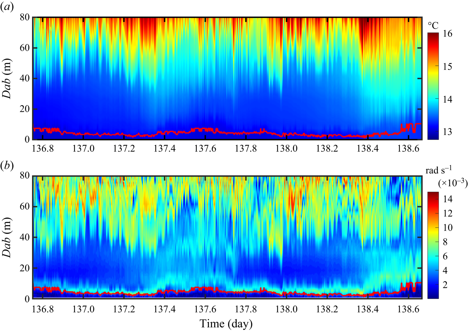
The BML is a quasi-homogeneous layer in the ocean characterized by uniform temperature, salinity, density and other properties (Weatherly & Martin Reference Weatherly and Martin1978; Shimizu Reference Shimizu2010; Trowbridge & Lentz Reference Trowbridge and Lentz2018; Huang et al. Reference Huang, Cen, Lu, Guo and Zhou2019, Reference Huang, Cen, Guo, Lu, Zhou, Qiu, Zhang, Wu and Han2021). By analysing the vertical temperature profiles detected from the densely distributed thermistors, we determine the thickness of the BML,  $H_{BML}$, and examine its evolution. To accurately determine the BML from less fluctuating profiles, the temperature is averaged every 60 s. The thickness
 $H_{BML}$ is computed as the distance from the bottom to the point where the potential temperature changes by 0.02
 $^{\circ }$C. In the observation period,
 $H_{BML}$ exhibits high intermittency, ranging from
 $0.8$ to 10.4 m, with an average of approximately 4.1 m. This confirms the persistent nature of the BML above the seafloor, consistent with previous reports (Qu et al. Reference Qu2021). Within the BML, the buoyancy frequency averages around 0.0018 rad s
 $^{-1}$, ranging from unstable stratification to 0.005 rad s
 $^{-1}$.
3.2. Scaling behaviour in the temperature spectrum
The precise temperature measurements available allow us to examine the scaling behaviour in turbulent oceanic conditions. The smallest turbulent scale can be assessed using the Kolmogorov time scale, defined as  $\tau _{\eta }=\sqrt {\nu /\varepsilon }$, where
 $\nu$ is the kinematic viscosity (Kolmogorov Reference Kolmogorov1941). For typical values on the shelf of the northern SCS,
 $\nu \sim 10^{-6}\ {\rm m}^2\ {\rm s}^{-1}$ and
 $\varepsilon \sim 10^{-8}\ {\rm m}^2\ {\rm s}^{-3}$ (St. Laurent et al. Reference St. Laurent, Simmons, Tang and Wang2011; Qu et al. Reference Qu2021), the estimated Kolmogorov time is approximately
 $\tau _{\eta }\sim 10$ s. Thus, all possible turbulent states, including the so-called inertial range, can be well resolved here (Frisch Reference Frisch1995).
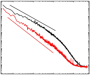
The temperature spectra in three layers, i.e. the BML, the mixing zone and the internal wave zone, are individually examined to learn the influences of different dynamic processes. To ensure sufficient statistics over a broad frequency range, all temperature data recorded within the same zone are depth-averaged, resulting in less fluctuating spectra. Figure 4 illustrates the power spectra for each layer. Within the BML, the temperature spectrum  $E_{\theta }$ exhibits a scaling behaviour in the frequency range
 $\langle N_{BML}\rangle <\omega <0.3$ rad s
 $^{-1}$, where
 $\langle N_{BML}\rangle$ is the averaged buoyancy frequency of
 ${\sim }0.002$ rad s
 $^{-1}$. The best data fitting yields a scaling exponent of
 $\alpha =-1.34\pm 0.07$. This scaling exponent is in close agreement with the theoretical prediction of BO scaling,
 $-7/5$ (Bolgiano Reference Bolgiano1959; Obukhov Reference Obukhov1959). Similar scaling laws have also been observed in recent studies of van Haren's group in the deep alpine Lake Garda (van Haren & Dijkstra Reference van Haren and Dijkstra2021), the deep slope at Mount Josephine in the northeastern Atlantic (van Haren Reference van Haren2022) and the deep western Mediterranean (van Haren Reference van Haren2023).
The averaged temperature spectra  $E_{\theta }$ in the internal wave zone (
 $Dab=[40, 80]$ m, blue), mixing zone (
 $Dab=[10, 40]$ m, red) and BML (
 $Dab=[0, H_{BML}]$, black), with the corresponding fitted power scalings of
 $-1.34$,
 $-1.69$ and
 $-2.12$. The vertical dashed lines indicate the nominal buoyancy frequency in the internal wave zone
 $\langle N_{iw}\rangle$, mixing zone
 $\langle N_{m}\rangle$ and BML
 $\langle N_{BML}\rangle$.

In the mixing zone, the temperature spectrum shows fluctuations at frequencies below the averaged buoyancy frequency of  $\langle N_m\rangle \sim 0.003$ rad s
 $^{-1}$, likely attributed to intermittent influences of internal waves. In the range
 $0.01<\omega <0.5$ rad s
 $^{-1}$, the spectrum exhibits a consistent scaling behaviour, with the best-fitted scaling exponent of
 $\alpha =-1.69\pm 0.07$. This scaling exponent is remarkably close to Kolmogorov's prediction (
 $-5/3$) for isotropic turbulence. The presence of the classical Kolmogorov scaling has been extensively observed in the ocean, as reported in Moum (Reference Moum2015), Becherer & Moum (Reference Becherer and Moum2017), Ewart (Reference Ewart1976), Klymak & Moum (Reference Klymak and Moum2007) and Holbrook & Fer (Reference Holbrook and Fer2005).
According to the classical BO phenomenology, the Bolgiano scale  $l_B$ is defined as
 $l_B=N^{-3/2}\varepsilon ^{5/4}\chi ^{-3/4}$, where
 $\varepsilon$ is the energy dissipation rate and
 $\chi$ is the temperature dissipation rate. The spectrum will be Kolmogorov-like for the length scale
 $l < l_B$ and BO-like for
 $l > l_B$. Here, the observation of Bolgiano scaling in the BML and Kolmogorov scaling in the mixing zone suggests that
 $l_B$ should be small near the ocean bottom and increase on moving away from the bottom when the BO theory is applicable. There has been little work on
 $l_B$ around the boundary layer in stratified turbulent flow. However, numerical simulations in turbulent thermal convections have shown a distribution similar to the present observation (Calzavarini, Toschi & Tripiccione Reference Calzavarini, Toschi and Tripiccione2002; Kunnen et al. Reference Kunnen, Clercx, Geurts, Bokhoven and Akkermans2008). In these studies, it is found that
 $l_B$ is small near the boundary and increases gradually when far from the boundary, corresponding to a transition from a BO-dominated regime near the wall to a Kolmogorov regime moving away from the boundary (Calzavarini et al. Reference Calzavarini, Toschi and Tripiccione2002).
In the internal wave zone, the water is more stratified with averaged buoyancy frequency  $\langle N_{iw}\rangle \sim 0.01$ rad s
 $^{-1}$. The clear single scaling shifts to a higher-frequency range of
 $0.02<\omega <1$ rad s
 $^{-1}$, with the best-fitted scaling exponent of
 $\alpha =-2.12\pm 0.15$. The presence of a
 $-2$ scaling in oceanography primarily reflects the canonical ocean-interior saturated internal wave, which occurs between the inertial frequency
 $f$ and the buoyancy frequency
 $N$. This frequency range is typically much smaller than the turbulent inertial range (Garrett & Munk Reference Garrett and Munk1972). Phillips (Reference Phillips1971) proposed that continuously breaking internal waves would leave a trail of locally mixed fluid in the travelling waves, and the fine structures are advected by large-scale internal waves, where the advection process leads to broadband contamination of Eulerian time series, resulting in a
 $-2$ scaling. A similar
 $-2$ scaling was also observed by van Haren (Reference van Haren2023) in the turbulence regime at approximately 100 m above the seafloor in the western Mediterranean, and they proposed that nonlinear interactions in internal waves may transfer their energy into irreversible turbulence, this spectral property being related to the chaos theory of Brownian noise (Schuster & Just Reference Schuster and Just2006).
4. Discussion
Extensive observations of the Kolmogorov scaling have been documented in the velocity or temperature spectra of the oceanic bottom boundary layer across various environments, including bays (Gross & Nowell Reference Gross and Nowell1985), tidal channels (Lien & Sanford Reference Lien and Sanford2004), continental shelves (Chriss & Caldwell Reference Chriss and Caldwell1984) and deep ocean (van Haren & Gostiaux Reference van Haren and Gostiaux2009). Recent studies by van Haren & Dijkstra (Reference van Haren and Dijkstra2021) and van Haren (Reference van Haren2022, Reference van Haren2023) have also reported the presence of BO scaling in the bottom ocean through precise temperature measurements, which is proposed to be associated with active scalar buoyancy-driven turbulent convection.
The applicability of the BO phenomenology in buoyancy-driven turbulent convection has sparked controversy. While some studies observed BO scaling, others report a Kolmogorov-like spectrum (e.g. Ahlers, Grossmann & Lohse (Reference Ahlers, Grossmann and Lohse2009), Lohse & Xia (Reference Lohse and Xia2010) and references therein). Recent arguments challenge the validity of the BO theory, suggesting that the total energy cascade cannot remain balanced under unstable stratification, contradicting the premise of BO theory (Kerr Reference Kerr1996; Kumar et al. Reference Kumar, Chatterjee and Verma2014; Verma, Kumar & Pandey Reference Verma, Kumar and Pandey2017).
Within the BML, the water experiences alternating weak and unstable stratification. Figure 5(a) shows the square of the buoyancy frequency  $N^2$ within the BML, indicating convective instability during two time periods (day [137.44, 137.58] and day [138.57, 138.67]), where
 $N^2$ is slightly less than zero. The convective process can be quantified using the Rayleigh number
 $Ra= g\Delta \sigma _{max} H_{BML}^3/(\rho _0\nu \kappa _\theta)$, where
 $\Delta \sigma _{max}=\alpha '\Delta \theta _{max}$ is the maximum negative density anomaly relative to the ocean bottom within the BML,
 $\nu$ (
 ${\sim }1.3\times 10^{-6}\ {\rm m}^2\ {\rm s}^{-1}$) is the kinematic viscosity and
 $\kappa _\theta$ (
 ${\sim }1.4\times 10^{-7}\ {\rm m}^2\ {\rm s}^{-1}$) is the molecular thermal diffusivity. The calculated range for
 $Ra$ falls between
 $10^9$ and
 $10^{11}$, comparable to values observed in laboratory and numerical experiments (Zhou, Sun & Xia Reference Zhou, Sun and Xia2007; Ching Reference Ching2014).
The nominal (a) buoyancy frequency squared,  $N^2$, and (b) Richardson number,
 $Ri$, in the mixing zone (
 $Dab=[10, 40]$ m, red) and BML (
 $Dab=[0, H_{BML}]$, black). In (a), instances of unstable stratified convection are marked with green shading. In (b), the grey dashed line at
 $Ri=0.25$ is for reference. (c) Temperature power spectra in the BML during the convection (red) and weak-stratification (black) phases, with the corresponding fitted scaling exponents of
 $-1.76$ and
 $-1.34$. (d) Temperature power spectra in the mixing zone during weak (black) and strong (red) stratifications, with the corresponding fitted scaling exponents of
 $-1.67$ and
 $-1.60$.

The BML temperature data are separated into two categories, unstable stratification and weak stratification, and the corresponding temperature spectrum of each state is computed. As shown in figure 5(c), the unstably stratified convection phase deviates significantly from the BO scaling of  $-7/5$. Instead, the best-fitting result yields
 $\alpha =-1.76 \pm 0.10$, which is closer to the classical scaling of
 $-5/3$ observed in isotropic turbulence. Previous studies in the atmospheric surface layer have argued that flow dynamics is dominated by both mechanical turbulence and convection under the unstable condition of
 $-0.03< Ri<0$ (Schnelle & Dey Reference Schnelle and Dey1999). During the observed unstable convection phases,
 $Ri$ is approximately
 $-3.6 \times 10^{-5}$ (see figure 5b), suggesting the possible significant contribution of turbulent shear too. During the rest of the time, the BML water exhibits a weakly stratified condition with a buoyancy frequency of
 $N \sim 0.0018$ rad s
 $^{-1}$. In these phases, the scaling
 $\alpha =-1.34\pm 0.10$ appears to follow the BO scaling rather than the Kolmogorov scaling.
Recent numerical simulation studies have suggested that the BO scaling occurs in moderately stratified conditions but not in near-neutral or very stable conditions (Kumar et al. Reference Kumar, Chatterjee and Verma2014; Verma et al. Reference Verma, Kumar and Pandey2017; Alam et al. Reference Alam, Guha and Verma2019). Turning our attention back to the mixing zone, as shown in figure 3(b), temporal variations in stratification are exhibited. During day  $[136.75,137.17]$ and day
 $[137.79,138.22]$, the stratification is weak with
 $N$ being approximately 0.0024 rad s
 $^{-1}$, and the fitted scaling
 $\alpha =-1.67 \pm 0.05$ is observed in the temperature spectrum (figure 5d). In the remaining time, the water exhibits relatively strong stability with an
 $N$ of 0.0047 rad s
 $^{-1}$, and the scaling
 $\alpha$ is fitted as
 $-1.60 \pm 0.10$ in the temperature spectrum. Notably, both the scalings are close to the Kolmogorov value of
 $-5/3$ rather than the BO scaling of
 $-7/5$.
The above results show that the scaling  $\alpha$ follows the BO-like scaling only in the case of weak stratification in the BML (
 $N\sim 0.0018$ rad s
 $^{-1}$). However, in the tightly closed weak stratification of the mixing zone (
 $N\sim 0.0031$ rad s
 $^{-1}$), the scaling adheres to the Kolmogorov-like scaling. This implies the presence of other forces at play. To gain further insights, the Richardson number
 $Ri$ is utilized, which characterizes the interplay between buoyant and shear forces in turbulent conditions. Since the LADCP cannot effectively measure the bottom current close to the seafloor, velocity data from the SeaGuard current meter at
 $Dab=2.2$ m were used to estimate the current shear and
 $Ri$ within the BML, assuming a no-slip boundary condition. As shown in figure 5(b),
 $Ri$ exhibits remarkable fluctuations in the BML. In the weakly stratified BML,
 $Ri \sim 0.0027$ is found, which is approximately two orders of magnitude smaller than the value (
 $Ri\sim 0.19$) in the mixing zone. This result might imply that the BML is in a more turbulent state and the combination of weak stratification and strong shear promotes a cascade scaling close to that of BO theory. In recent large-eddy simulations of stratified turbulence, it has been found that the BO theory is valid in moderate stratification at
 $Ri\sim 10$, while the Kolmogorov scaling is followed in strong stratification at
 $Ri \sim 25$ (Agrawal & Chandy Reference Agrawal and Chandy2021). However, in other high-resolution direct numerical simulations (Kumar et al. Reference Kumar, Chatterjee and Verma2014; Alam et al. Reference Alam, Guha and Verma2019), it is reported that BO scaling is valid for
 $Ri\sim 1$ but Kolmogorov scaling is valid for
 $Ri=4\times 10^{-7}$. In these simulations,
 $N$ typically remains constant and is set to unity. It is essential to exercise caution when comparing these numerical results with the current observations. Basu & Bhattacharjee (Reference Basu and Bhattacharjee2019) also pointed out that
 $N$ is an important control parameter for producing different scaling regimes. The current results suggest that both stratification and turbulent intensity are key factors in buoyancy-driven turbulent scaling behaviours, providing insights for future study.
5. Conclusions
In summary, we examine the turbulent cascade scalings in the bottom ocean using high-resolution temperature data from a mooring in the northern SCS. The bottom water exhibits three distinct structures in terms of stratification variability, which are classified as the BML, the mixing zone and the internal wave zone with increasing distance from the seafloor. In the weak stratification phase of the BML, a scaling of  $-1.34\pm 0.10$ is observed, which is close to the prediction of the BO theory. The similar cascading behaviours in the oceanic bottom boundary layer and the atmospheric surface layer might suggest common underlying mechanisms driving turbulent states, which merits further study. However, in the unstably stratified convective turbulence within the BML, the scaling of
 $-1.76\pm 0.10$ deviates from the BO theory and appears closer to the classical scaling of
 $-5/3$ in isotropic turbulence, suggesting that the convective turbulence is not the promise of BO scaling. In the mixing zone, the water remains in weakly stable stratification, although it exhibits alternating weak and strong stratification in the diurnal cycle. The scaling is observed to be closer to the Kolmogorov scaling of
 $-5/3$. The Richardson number in the mixing zone is around
 $0.25$, which is approximately two orders of magnitude larger than that in the BML. Under similar weak stratifications, the scaling comparison in the BML and the mixing zone suggests that strong shear flow promotes the occurrence of BO-like scaling, while weak shear leads to Kolmogorov-like scaling. In the internal wave zone, the more stable stratification is significantly modulated by the intense internal waves. A scaling of
 $2.12\pm 0.15$ is observed in the frequency range higher than the averaged buoyancy frequency
 $N$ within this region (
 $\omega > N$). Although the
 $-2$ scaling has been extensively observed in the internal wave frequency range (
 $\omega < N$), the present observation of turbulent states requires further clarification, despite the suggested possible mechanisms as continuously breaking internal waves (Phillips Reference Phillips1971) and chaos theory of Brownian noise (Schuster & Just Reference Schuster and Just2006).
Acknowledgements
Those who helped to collect, calibrate, process and archive the GEBCO grid dataset are appreciated. Data were collected onboard R/V Jiageng implementing the open research cruise NORC2018-06 supported by NSFC Shiptime Sharing Project (project number 41749906).
Funding
This work was supported by the National Key Research and Development Program of China (2021YFC3101300), the National Natural Science Foundation of China (NSFC) (42006196, 42206020, 12172369, 42249907, 42449907), the Basic and Applied Basic Research Foundation of Guangdong Province (2021A1515110839), the Hainan Provincial Natural Science Foundation of China (422QN439), the Science and Technology Projects in Guangzhou (2024A04J4049), the State Key Laboratory of Tropical Oceanography, South China Sea Institute of Oceanology, Chinese Academy of Sciences (LTO2219) and the Hubei Provincial Natural Science Foundation of China (2022CFB334).
Declaration of interests
The authors report no conflict of interest.
Data availability statement
The data that support the findings of this study are openly available in Figshare at https://figshare.com/articles/dataset/2020Dongsha_tripod/25149068.



