


1. INTRODUCTION
Velocity fields of tidewater glaciers are sensitive indicators of the various driving and resisting forces acting upon them (e.g. Howat and others, Reference Howat, Joughin, Fahnestock, Smith and Scambos2008). Unfortunately, it is challenging to obtain such data with adequate spatial and temporal resolution. Discrete GPS measurements undersample the velocity field in a spatial sense. Satellite observations give a well-resolved two-dimensional (2-D) (horizontal) velocity field via feature or speckle tracking (e.g. Joughin and others, Reference Joughin2008; Ahn and Howat, Reference Ahn and Howat2011) but undersample the temporal variation. Temporal resolution of ice velocity from spaceborne sensors is generally limited to several days or more and thus undersamples short-term fluctuations in the highly dynamic zones of marine-terminating glaciers, where iceberg calving and changes in basal water pressure may be frequent and lead to rapid stress and velocity variations.
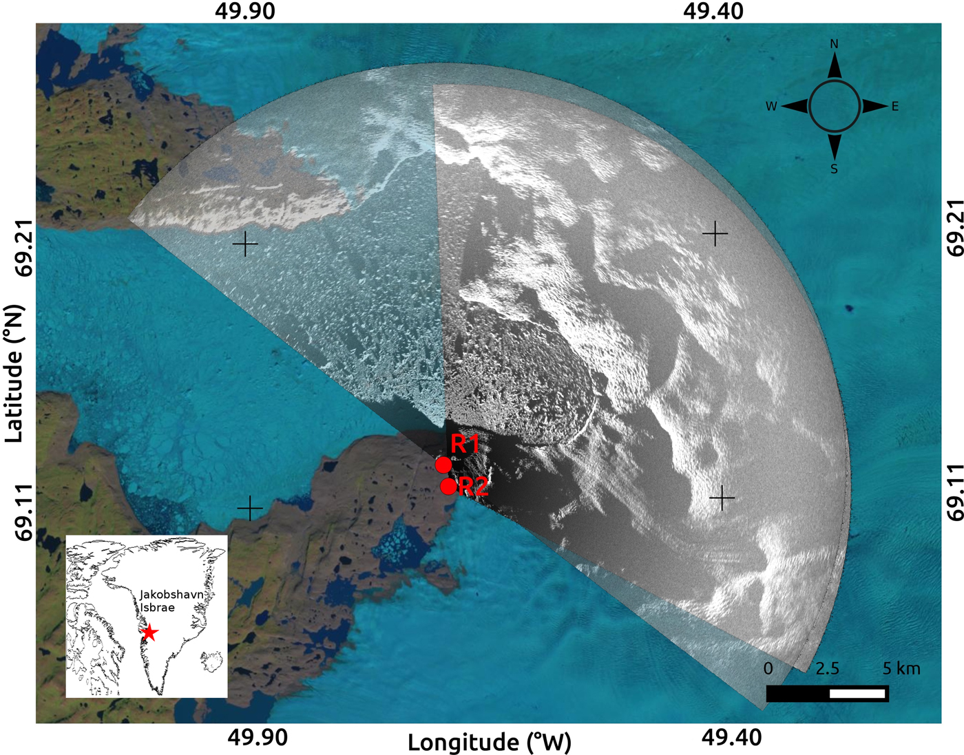
Jakobshavn Isbrae is an outlet glacier on the west coast of Greenland (Fig. 1). The main trunk of the glacier is ~5 km wide and moves at ~40 m d−1 (Amundson and others, Reference Amundson2010) with cliff heights of ~100 m (Xie and others, Reference Xie2016). Jakobshavn drains ~6% of the Greenland ice sheet (Bindschadler, Reference Bindschadler1984) and is likely to have accounted for ~4% of the increase in sea-level rise rate for the 20th century (Houghton and others, Reference Houghton2001). It represents an important target for research aimed at understanding the overall health of the Greenland ice sheet.
Map of the field area. Site location relative to Greenland marked by red star (inset). R1 and R2 show the locations of the TRI instruments. Their respective coverage areas are shown by overlapping gray scales, overlain on a LANDSAT image from 11 August 2014 (obtained from landsatlook.usgs.gov).
Terrestrial radar interferometers (TRIs) have been used to study a variety of geophysically deforming surfaces at very high (minute-scale) sampling rates. Caduff and others (Reference Caduff, Schlunegger, Kos and Wiesmann2015) and Voytenko and others (Reference Voytenko2015a) review the basic TRI technique. Voytenko and others (Reference Voytenko2015c) used near-field TRI observations to resolve the vertical component of deformation along a tidewater glacier terminus. Xie and others (Reference Xie2016) observed a calving event at Jakobshavn using a TRI. Feature-tracking techniques have been applied to TRI observations of Jakobshavn's proglacial fjord (Peters and others, Reference Peters2015). However, such techniques have limited temporal resolution compared with interferometric measurements (hour vs minute-scale) or require very fast motion (e.g. ice mélange during a calving event). Although a single instrument provides only scalar line-of-sight (LOS) measurements, in principle, measurements from two identical synchronized TRIs positioned at different locations but observing a common overlapping area can be combined to define both horizontal components of glacier velocity.
In this study, our TRIs are real-aperture Ku band (1.74 cm wavelength) GAMMA Portable Radar Interferometers (GPRI) (Werner and others, Reference Werner, Strozzi, Wiesmann and Wegmüller2008). Each instrument has three antennas (one transmitting and two receiving). The receiving antennas have a 25 cm baseline, and the transmitting and lower receiving antenna (which are the ones used in this study) have a 60 cm baseline, which allow for displacement sensitivity of ~1 mm and an elevation sensitivity of 3 m at a distance of 2 km (Strozzi and others, Reference Strozzi, Werner, Wiesmann and Wegmuller2012). The antennas are attached to a rotating frame and scan an arc of a specified angle to image the scene. The maximum range of our TRIs is ~16 km, with a nominal range resolution of 0.75 m and an azimuth resolution of 7 m at 1 km, which linearly widens with distance. TRIs are designed for installation on stable bedrock. Deployments on moving ice are logistically difficult, complicate the measurements, and thus are not ideal. Because the TRI does not move in space during a study period, no topographic phase correction is required when processing the interferograms.
Methods to obtain components of motion from two viewpoints have been developed for weather radars (Lhermitte and Miller, Reference Lhermitte and Miller1970) and subsequently for satellite synthetic aperture radar data from ascending and descending passes (Joughin and others, Reference Joughin, Kwok and Fahnestock1998; Fialko and others, Reference Fialko, Sandwell, Simons and Rosen2005). Here, we present a similar TRI-based approach to resolve the two horizontal components of the surface velocity field at Jakobshavn.
2. METHODS
2.1. Derivation of equations to combine data from two radars
Consider a parcel of glacier ice that is moving in two dimensions and is seen by two radars (TRIs). Assume that the vertical motion is insignificant. The components of the velocity vector of the parcel with respect to east and north are V x and V y. The TRI, however, only measures the velocity of the parcel in the direction of its LOS, with V R1 representing the LOS velocity measured by TRI 1, and V R2 representing the LOS velocity measured by TRI 2. The LOS angles (measured counterclockwise from east by convention) for each azimuth line are θ 1 and θ 2 for TRIs 1 and 2, respectively (Fig. 2).
Diagram of the field set-up for the derivation of Eqn (1). Radar positions are R1 and R2 (triangles), LOS velocities measured with each radar are V R1 and V R2, angles from the radars to a parcel of interest on the glacier (stars) are θ 1 and θ 2 (dashed lines). True velocity of an ice parcel observed by the radar on the glacier is V glac, and its north and east components are V y and V x. Vectors of the radars are given by the dotted lines originating from radars toward the parcel of interest. V x and V y are obtained using the measured V R1 and V R2 and the known (from the instrument locations) θ 1 and θ 2. Note that the LOS velocities (V R1 and V R2) are obtained from a vector projection of V glac onto the look vectors of R1 and R2. Also note that if the glacier is moving toward the radar, the measured velocity is negative because the distance (slant range) is decreasing between the first and second image in the interferogram.
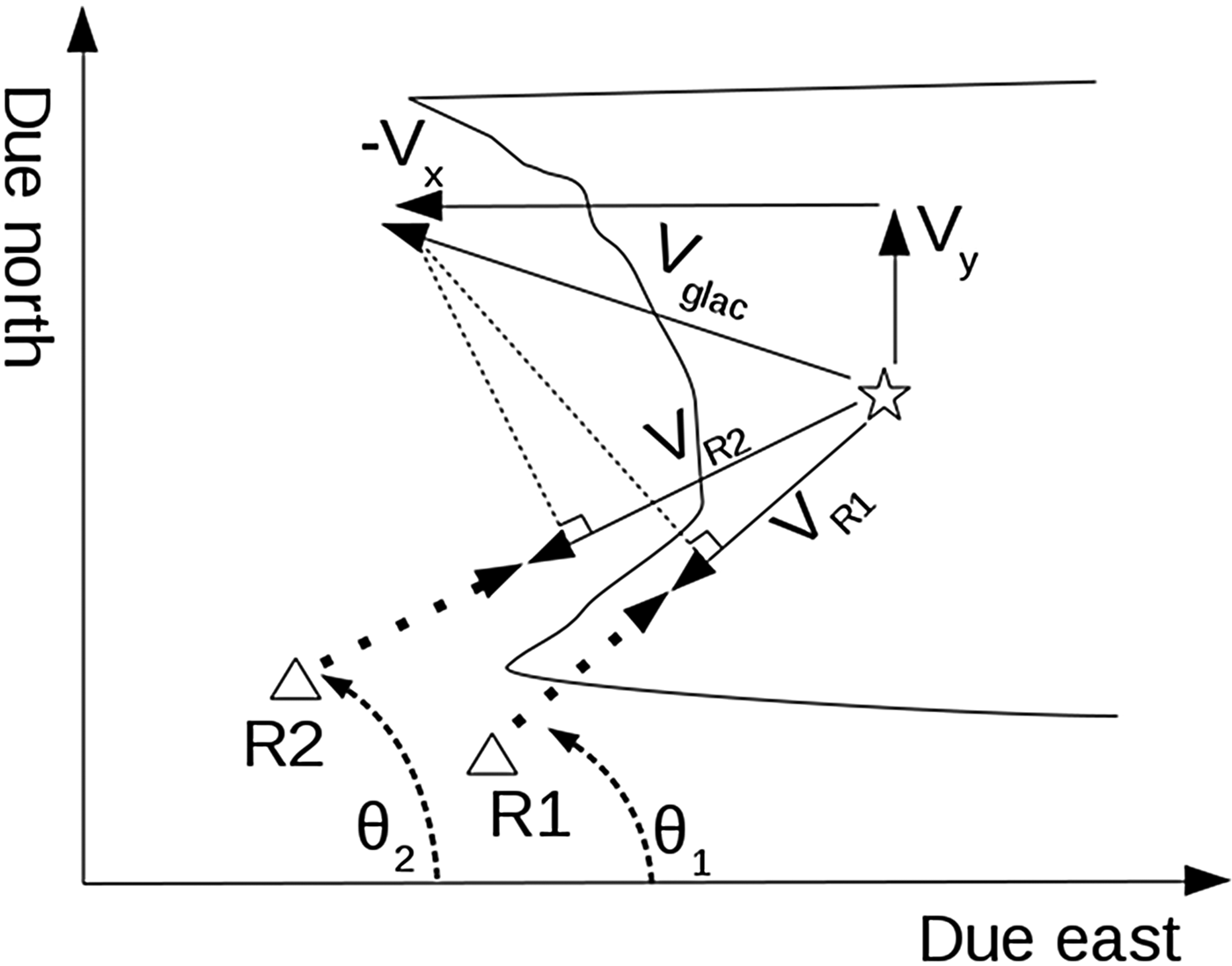
We derive an equation describing the measured LOS velocity as a function of V x and V y of the parcel and the LOS angle of the TRI, θ. We do this by rotating the coordinate system of a given vector [V x, V y] by the angle θ.
 $$\left[ {\matrix{ {V^{\prime}_x} \cr {V^{\prime}_y} \cr}} \right] = \left[ {\matrix{ {{\rm cos}(\theta )} & {{\rm sin}(\theta )} \cr { - {\rm sin}(\theta )} & {{\rm cos}(\theta )} \cr}} \right]\left[ {\matrix{ {V_x} \cr {V_y} \cr}} \right].$$
Note that V′x is the component of velocity in the direction of the unit vector given by θ, which happens to be the velocity component measured by the TRI. Since this is the only component measured by the TRI, we can ignore the other component of rotation (V′y), and obtain an equation for the measured radial velocity:
 $$V_R = V_x {\rm cos}(\theta ) + V_y {\rm sin}(\theta ).$$
Therefore, the velocity equations for both TRIs are:
 $$V_{R1} = V_x {\rm cos}(\theta _1 ) + V_y {\rm sin}(\theta _1 ),$$
 $$V_{R2} = V_x {\rm cos}(\theta _2 ) + V_y {\rm sin}(\theta _2 ).$$
The above equations are sufficient to generate a forward model for the dual TRI velocity problem.
In reality, the two TRIs measure V R1 and V R2, where θ 1 and θ 2 are the instrument look angles, and are known from the locations of the instruments and the georeferenced images. The focused TRI images are by default in polar coordinates, where one axis is azimuth (an angular measure of the scan) and the other is slant range (distance from the origin, measured as the shortest distance from radar to target). Therefore, we can rewrite the TRI velocity equations in the A x = b form, and solve for V x and V y for each point using matrix inversion.
 $$\left[ {\matrix{ {V_x} \cr {V_y} \cr}} \right] = \left[ {\matrix{ {{\rm cos}(\theta _1 )} & {{\rm sin}(\theta _1 )} \cr {{\rm cos}(\theta _2 )} & {{\rm sin}(\theta _2 )} \cr}} \right]^{ - 1} \left[ {\matrix{ {V_{R1}} \cr {V_{R2}} \cr}} \right].$$
The inverse matrix can be written explicitly with no numerical inversion required:
 $$A^{ - 1} = \displaystyle{1 \over {det(A)}}\left[ {\matrix{ {{\rm sin}(\theta _2 )} & { - {\rm sin}(\theta _1 )} \cr { - {\rm cos}(\theta _2 )} & {{\rm cos}(\theta _1 )} \cr}} \right],$$
where det(A) = [cos(θ 1)sin(θ 2) − sin(θ 1)cos(θ 2)] = sin(θ 2 − θ 1).
2.2. Data acquisition and processing
We set up two TRI instruments on the south side of the Ilulissat fjord ~6 km from the terminus of Jakobshavn Isbrae (Fig. 1) and collected data with a 3 min sampling interval. The radar separation was ~1 km, constrained by local geography. One radar was at an elevation of 314 m and the other one was at 270 m. A built-in GPS receiver provides accurate clock information to the TRI. Because of the 3 min sampling rate, we set the acquisition start times on both instruments to be the same (as opposed to being offset by 1 or 2 min). We use a single acquisition pair (2012/08/01 20:01 and 2012/08/01 20:04) to demonstrate the concept of our method, and compare the results with a longer 3-day period (2012/07/31 16:05 to 2012/08/03 16:06) of motion derived by feature tracking.
We prepare the interferograms from non-resampled single-look complex files using the GAMMA software package. During processing, we multilook (spatially average) the TRI data by 12 looks (averaged pixels) in range, smooth the interferograms with an adaptive filter (Goldstein and Werner, Reference Goldstein and Werner1998), set a phase unwrapping mask focused on the stationary rocks and the main trunk of the glacier (ignoring the ice mélange), and unwrap the phase using a minimum cost flow algorithm. We then convert the unwrapped interferograms (and the multilooked intensity images) into rectangular coordinates with 15 m pixel spacing. This conversion is needed for georeferencing to properly define the angles relative to due east. Due to the small elevation differences between the TRIs and the glacier (~200 m over a horizontal distance of ~5 km, suggesting an incidence angle of ~ 2°), we do not perform a terrain correction for conversion from slant range to ground range. The interferograms are then converted into velocities via a multiplicative factor of − λ/4πΔt, where λ is the wavelength (1.74 cm for the GPRI) and Δt is the time between the images in the interferogram (3 min in our case).
One of the radar datasets suffers from phase unwrapping issues, likely due to the look direction of the radar relative to the principal direction of glacier motion and the 3 min sampling rate. We correct for this by manually adjusting the resulting unwrapped interferogram by two cycle slips and recalculating the velocity (this offset is determined by examining an area where the look angles of both radars are similar, and should measure similar rates). The intensity images are then compared with LANDSAT images and adjusted 39o and 59o for rotational offsets related to instrument locations, allowing for accurate calculation of the horizontal viewing angle. These offsets are determined by iteratively adjusting a rotation angle of a georeferenced image until some salient features (typically rock outcrops) visually overlap with the same features in a LANDSAT image. After georeferencing both velocity datasets to the same image space, we calculate θ 1 and θ 2 for each overlapping pixel using the radar pixel coordinates and the pixel coordinates containing the velocity values measured by each radar, and solve for the east and north components of velocity using Eqn (5) and the analytically derived inverse matrix in Eqn (6).
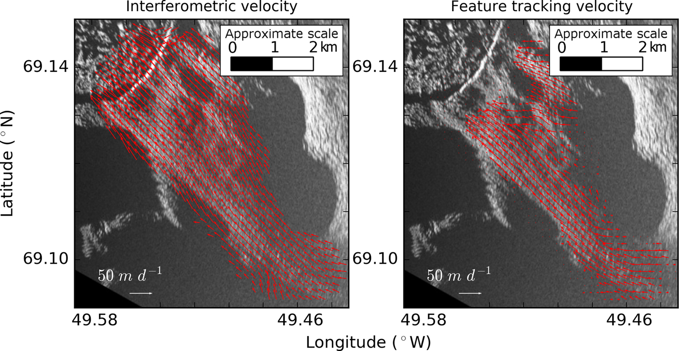
We use the correlation-based OpenPIV (particle image velocimetry) package (Taylor and others, Reference Taylor, Gurka, Kopp and Liberzon2010) to measure offsets over a 3-day period from the TRI images to compare our results. Here, the georeferenced intensity images have 5 m pixel spacing with a search window of 64 pixels and an overlap of 32 pixels. The output of each velocity component is smoothed with a 5-pixel median filter. We then resample the resulting interferometric velocity component maps to the dimensions of the feature-tracking data and smooth them with a 5-pixel median filter for comparison (Figs 3, 4).
Plots of ice velocity derived from the 3 min interferometric data pair (left) and the 3-day feature tracking (right). The velocity magnitudes and directions are similar. The feature-tracking data are truncated near the terminus due to a calving event.
A pointwise comparison between the overlapping 2-D interferometric and feature-tracking data for components >5 m d−1. The plots compare eastward velocity (a), northward velocity (b), azimuth (c) and velocity magnitude (d). One-to-one relationship lines are shown on every plot. Note that the variability is close to what is described by the Monte Carlo simulation (Figs 6, 7). Error bars show the one SD uncertainties for the interferometric data. The feature-tracking (PIV) uncertainty is assumed to be 0.1 pixels (Huang and others, Reference Huang, Dabiri and Gharib1997), which, in this case, is 0.2 m d−1 (0.5 m over a 3-day period, to one significant figure) for each of the velocity components. The feature-tracking uncertainty error bars for the magnitude and azimuth are derived from another Monte Carlo simulation.

We combine the above method with a Monte Carlo simulation to perform uncertainty analysis, offering a more convenient alternative to error propagation (which would require calculating partial derivatives). The Monte Carlo method (Fig. 5) estimates the probability distribution of the solution by repeatedly solving the equations by sampling from the known or, more commonly, assumed probability distributions of the input parameters. Here, these are the radar LOS velocities, their orientations and their respective standard deviations (SDs). A large enough number of runs are performed to generate meaningful distribution statistics. Here, the results are the velocity components, where each component has its own probability distribution with a mean and SD.
A visual example of a Monte Carlo simulation (1000 runs) for a single point on the glacier surface. Here, the inputs are the radar velocity measurements (V R1 and V R2) and their respective view directions (θ 1 and θ 2). Note that we only obtain the distributions of V x and V y using the simulation. We then calculate the azimuth and velocity magnitude along with their respective uncertainties from the results of the simulation. This process is repeated for every desired data point over the glacier surface to produce Figures 6, 7.
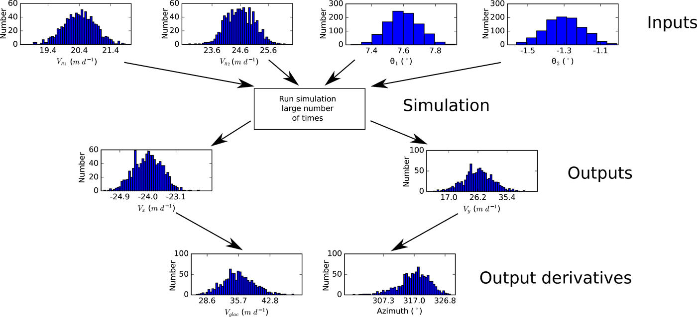
We assume that there are no phase unwrapping errors (from inspection and after accounting for the offset mentioned earlier) and that the radar-derived velocity and angle values are normally distributed with SDs of 0.5 m d−1 derived from on-rock TRI measurements at Breiðamerkurjökull (Voytenko and others, Reference Voytenko2015b) and 0.1° (the smallest eye-detectable difference when manually georeferencing the TRI image to a background LANDSAT image; the TRI azimuth positioner errors are negligible), respectively. We then run a simulation with 1000 samples for every measurement point and calculate the resulting ‘average’ velocity (in a probabilistic sense) along with an uncertainty (SD) for each component (Fig. 6). We then use the resulting data to obtain the best estimate and uncertainty of the principal direction of glacier motion (azimuth, given by  $90{\rm ^\circ} - \arctan (V_y /V_x )$) and the velocity magnitude (given by
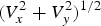 $(V_x^2 + V_y^2 )^{1/2} $) (Fig. 7).
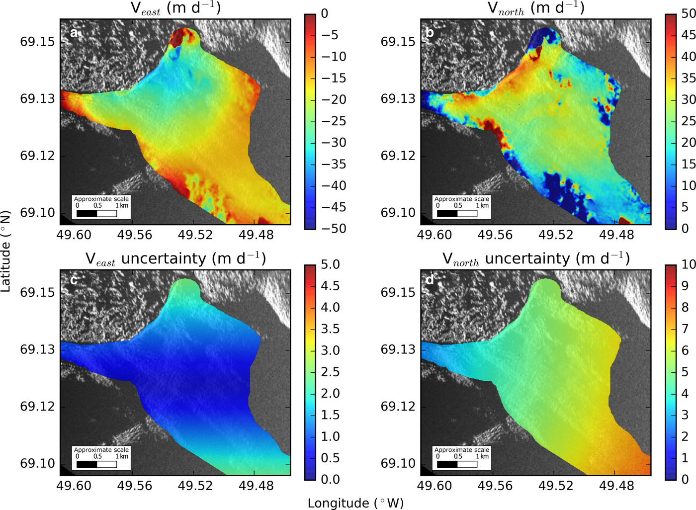
East (a) and north (b) velocity component maps and their uncertainties derived from interferometry and the Monte Carlo simulation. Note that northward uncertainties (d) are higher than eastward uncertainties (c), likely due to the scan orientations of the two TRIs.
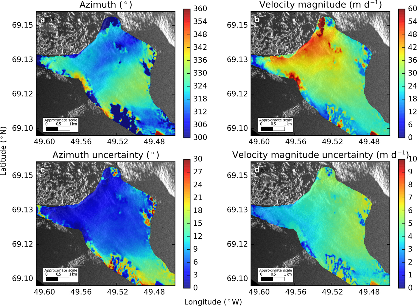
Direction and velocity magnitudes derived from interferometry (a, b) and their respective uncertainties (c, d) are all calculated from the Monte Carlo simulation. Note that azimuth is defined to be positive clockwise from north.
Since our method involves matrix inversion, we also need to consider precision loss due to the conditioning of the system (Atkinson, Reference Atkinson2008). The condition number (κ) represents the orthogonality of the system (a high condition number implies that the vectors inside the matrix are not orthogonal and that a small perturbation of the inputs will result in a large change in the outputs). A condition number of 1 implies orthogonality. We use the condition number of A, the matrix to be inverted (see the matrix of coefficients in Eqns (5) and (6)), and an L 2 norm to estimate precision loss for our 2-D velocity results. Note that the matrix only depends on the orientation of the two radars (i.e. the instrument locations and not the actual velocity measurements). In our case, A is ill conditioned when the look angles of the TRIs are similar.
 $$\kappa = {\rm \parallel} A{\rm \parallel} _2 {\rm \parallel} A^{ - 1} {\rm \parallel} _2. $$
Following the equation below, we calculate C, the number of digits of precision loss.
 $$C = \mathop {\log} \nolimits_{10} \kappa. $$
3. RESULTS AND DISCUSSION
Most of the ice around the study area flows to the northwest with an azimuth of ~315° and uncertainties (one SD) of ± 5° close the terminus and up to ±15° further up-glacier with velocity magnitudes ranging from ~50 m d−1 near the ice front to ~25 m d−1 up-glacier with uncertainties ~ ±6 m d−1 (Figs 3, 6, 7). The Monte Carlo simulation suggests that east-west uncertainties are ~1 m d−1, while north-south uncertainties are ~6 m d−1 (Fig. 6). This is likely due to the positioning of the radars relative to the main trunk of the glacier, their limited spatial separation (constrained by our site) and the scan orientations.
The interferometric and feature-tracking techniques yield similar magnitudes and directions (Fig. 4), except for slight discrepancies in the direction of motion where interferometric azimuth is systematically ~15° greater than the feature-tracking azimuth. This may be due to different sampling periods, measurement uncertainties and the conditioning of the equations. Additionally, the interferometric results are based on a 3 min period, while the feature-tracking results cover a 72 h period and include a calving event, which could affect the average direction of ice motion and its velocity magnitude (Amundson and others, Reference Amundson2008; Nettles and others, Reference Nettles2008).
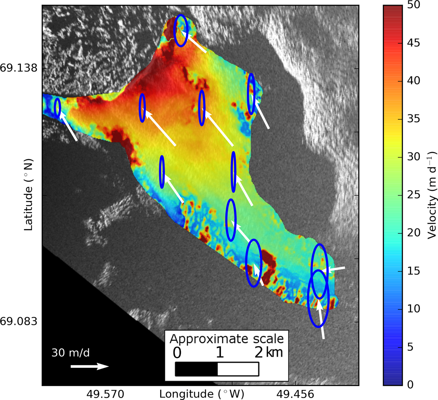
We also use the Monte Carlo simulation results to plot error ellipses (covering two SDs) for a selected subset of points (Fig. 8). The method of plotting the error ellipses depends on the uncertainty of each component (in this case, obtained from the Monte Carlo simulations) and a desired confidence interval for the ellipse and is described in detail by Haug (Reference Haug2012) and Voytenko and others (Reference Voytenko2015b). Note that the shape of the error ellipses agrees with the uncertainties presented in Figure 6.
Plot of error ellipses for a selected subset of points over the glacier surface overlain on a map of velocity magnitude derived from interferometry. The ellipses (blue) cover two SDs and are scaled relative to the arrows (white) showing the direction of motion and speed. Note that the north uncertainty is much greater than the east uncertainty.
While examining the condition number of the system of equations, we note that when C is 10, we lose one digit of precision. Considering our previous velocity measurement uncertainty assumption of ±0.5 m d−1 (i.e. our measurements are precise to the ones decimal place), losing one decimal place of precision means that the resulting velocity is only accurate to the tens decimal place, or ±5 m d−1.
Given our instrument locations, most of the terminus loses a little over one digit of precision (Fig. 9), suggesting uncertainties of at least 5 m d−1 for each component, which are more conservative than the uncertainties computed from the Monte Carlo simulation (~1 to ~6 m d−1) (Fig. 6).
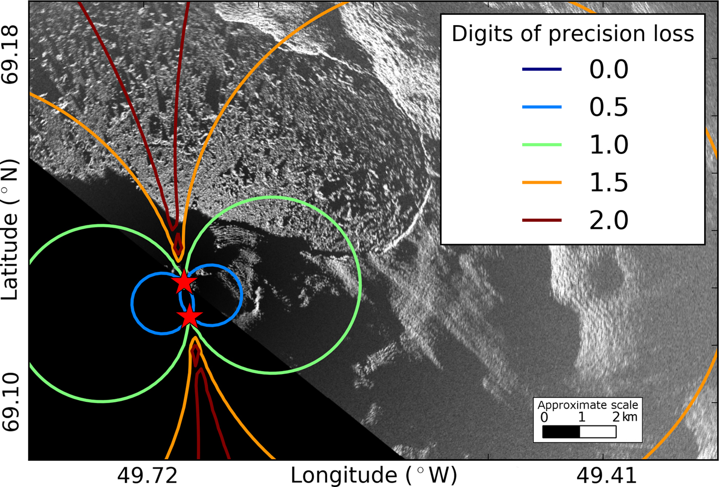
At Jakobshavn, locations for both radars that would be optimal for this method are either covered with glacier ice or are close to 16 km away from the terminus (near the useful range of the instrument), making 2-D interferometric measurements with TRI challenging at this location. However, since these precision loss calculations only depend on the instrument locations, they can be used in a forward model prior to future deployments to determine suitable instrument positions at other sites. For applications involving imaging the calving front of marine-terminating glaciers, if geography and logistics allow, the optimum radar separation should be such that the two radars are imaging the target area at close to right angles (to improve the conditioning of the system of equations) and within the operating range of the instruments.
4. CONCLUSIONS
Our work shows that it is possible to obtain minute-scale 2-D velocity fields using TRI. Although feature tracking can be used to obtain 2-D velocity fields from pairs of intensity images from a single radar, the results are likely to cover multiple hours of motion. Instead, our algorithm can be used to obtain results over minute-scale time steps using two radars. This method should be applicable in any location where a favorable site geometry exists. Salient features (e.g. bare rocks), which are visible in the TRI and the background (e.g. LANDSAT) imagery, are also required for visual georeferencing.
Based on results from our deployment and the analysis presented above, we can define an improved experiment design that should yield a robust 2-D glacier velocity field in most situations.
First, the two radars should be spatially separated by an amount such that there is sufficient angular separation for most of their overlapping image areas. Optimal radar placement can be determined before field deployment by modeling radars at different locations and calculating the expected precision loss via the condition number. Ideally, the radar look directions should be perpendicular over the region of interest, the area of which should be well within the ~16 km operating range.
Second, the time interval between radar scans, which should be identical for the two instruments, should be sufficiently short such that phase unwrapping can be done accurately (as close as possible to yield a displacement of half of a wavelength, while letting the radar scan a large enough arc to cover the area of interest). For fast moving glaciers such as Jakobshavn, 1½–2 min TRI scans may be optimum. In our 2012 experiment, we used 3 min scans. This longer time scan may have contributed to some of the phase unwrapping problems we encountered.
Having frequent and spatially dense coverage of 2-D glacier surface velocities at the terminus is necessary to improve our understanding of the calving process. Since GPS deployments on rapidly moving ice are logistically difficult, costly and sparse, and satellite measurements do not have minute-scale revisit times, a combination of two TRI instruments can provide the necessary spatial and temporal resolution.
ACKNOWLEDGEMENTS
We thank editor Hamish Pritchard, Reinhard Drews and an anonymous reviewer for their valuable comments. We thank the Gordon and Betty Moore Foundation and NASA's Cryospheric Sciences program. T.H.D. acknowledges support from NASA grant NNX12AK29G. R.C. acknowledges support under the NASA Earth and Space Science Fellowship (NNX14AL29H). D.M.H. and D.V. acknowledge support of NYU Abu Dhabi Research Institute grant G1204, as well as from NASA through the ‘Oceans Melting Greenland’ program led by JPL with subcontract to NYU and thank support from NSF Polar Programs ARC-1304137.



 Open access

