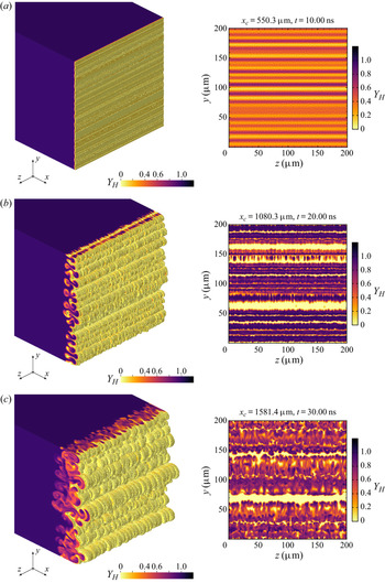
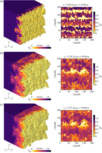
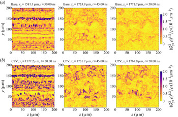
1. Introduction and background
Shock-induced multimaterial mixing is an important canonical process in fluid mechanics. It occurs in many flows of contemporary physics and engineering interest, such as capsule implosions for inertial confinement fusion (ICF), fuel–air combustion in scramjet-powered hypersonic vehicles and supernovae explosions. When the interface between two different-density fluids is shocked, initial perturbations grow via the Richtmyer–Meshkov (RM) instability (Richtmyer Reference Richtmyer1960; Meshkov Reference Meshkov1969; Brouillette Reference Brouillette2002). The RM instability can be compared with the Rayleigh–Taylor (RT) instability (Rayleigh Reference Rayleigh1883; Taylor Reference Taylor1950; Sharp Reference Sharp1984), which occurs whenever a low-density fluid is accelerated towards a high-density fluid. In complex flows, both the RM and RT instabilities (and others) may contribute to interpenetration and mixing.
For an archetypal flow driven by these instabilities, with small initial perturbations at a single light–heavy fluid interface, the evolution can be roughly divided into four phases. First, in the linear growth phase, described by linear theory (Chandrasekhar Reference Chandrasekhar1961; Atzeni & Meyer-ter-Vehn Reference Atzeni and Meyer-ter-Vehn2004), amplitudes  $\{\eta _i\}$ remain small relative to wavelengths
 $\{\lambda _i\}$, and the spectral modes evolve independently. Second, in the nonlinear growth phase, the
 $\{\eta _i\}$ are no longer small compared to the
 $\{\lambda _i\}$, but there is little interaction between different modes. Third, in the transitional phase, coupling between different modes becomes significant and vortical structures form. Fourth, in the turbulent phase, the flow exhibits chaos and a broad spectrum of length scales. The process of turbulent mixing can itself be divided into three sub-phases: entrainment, stirring and molecular mixing (Eckart Reference Eckart1948; Dimotakis Reference Dimotakis2000). Recent comprehensive reviews of the RM and RT instabilities and their association with mixing are available (Zhou Reference Zhou2017a,Reference Zhoub; Zhou et al. Reference Zhou, Clark, Clark, Glendinning, Skinner, Huntington, Hurricane, Dimits and Remington2019).
This paper discusses a computational investigation of shock-induced mixing at high energy density (HED), a term referring to thermodynamic pressures greater than 1 Mbar (Drake Reference Drake2018). The flows under consideration were realized in a series of experiments or shots at the National Ignition Facility (NIF) (Moses et al. Reference Moses, Boyd, Remington, Keane and Al-Ayat2009) as part of the experimental–computational Reshock Campaign introduced by Nagel et al. (Reference Nagel2017). In each experiment, two opposing laser-driven shock waves propagated through a millimetre-scale target package, which included a multimode rippled interface between two different-density solid materials. The solids were converted to plasmas, and the interface was impacted by a first shock and a subsequent reshock. Observations were made of the resulting mixing layer using X-ray radiography. In this paper, we present the design and analysis of a set of idealized three-dimensional (3-D) simulations of these experiments using the radiation hydrodynamics code Ares. We demonstrate that the simulations are consistent with the available experimental data. Then, we examine the evolution of key fluid-mechanical quantities in the simulated mixing layers, elucidating the unique physics of mixing at extreme conditions.
The Reshock Campaign was conceived as an HED analogue of studies of shock-induced instabilities and mixing at non-HED conditions. Such studies include many important experiments, several of which we highlight here. In each of the following examples, a shock tube was filled with two initially separated gases of different density. The interface between the gases was shocked, and measurements were made of the resulting mixing layer using various diagnostic techniques such as schlieren photography or planar Mie scattering. Reshock was due to reflection of the first shock off the tube endwall. Andronov et al. (Reference Andronov, Bakhrakh, Meshkov, Mokhov, Nikiforov, Pevnitskiĭ and Tolshmyakov1976) conducted one of the earliest of these experiments, measuring the width of an air–helium mixing layer over time. Vetter & Sturtevant (Reference Vetter and Sturtevant1995) diagnosed air–SF $_6$ mixing layers, finding that post-reshock mixing-layer growth rates were in good agreement with the theoretical model of Mikaelian (Reference Mikaelian1989) and were relatively insensitive to the initial configuration of an interfacial membrane. Houas & Chemouni (Reference Houas and Chemouni1996) investigated the effect of membrane thickness using various combinations of gases. Poggi, Thorembey & Rogriguez (Reference Poggi, Thorembey and Rogriguez1998) made novel measurements of instantaneous velocities in an SF
 $_6$–air mixing layer, reporting a substantial amplification of velocity fluctuations after reshock. Leinov et al. (Reference Leinov, Malamud, Elbaz, Levin, Ben-Dor, Shvarts and Sadot2009) examined air–SF
 $_6$ mixing layers, demonstrating that post-reshock growth rates were more sensitive to the strength of the reshock than to its time of arrival at the singly shocked layer. All of the aforementioned examples used a membrane for initial gas separation. Jacobs et al. (Reference Jacobs, Krivets, Tsiklashvili and Likhachev2013), building on work by Collins & Jacobs (Reference Collins and Jacobs2002), performed a membrane-less experiment in which an air–SF
 $_6$ interface was formed as a flow stagnation surface in a vertical shock tube. Other membrane-less experiments (Balakumar et al. Reference Balakumar, Orlicz, Tomkins and Prestridge2008, Reference Balakumar, Orlicz, Ristorcelli, Balasubramanian, Prestridge and Tomkins2012) investigated a thin SF
 $_6$–acetone gas curtain suspended in air. Balakumar et al. (Reference Balakumar, Orlicz, Ristorcelli, Balasubramanian, Prestridge and Tomkins2012) concluded that measured velocity fluctuations were consistent with the hypothesis that post-reshock mixing acted to reduce first-shock-induced anisotropy. Note that we have restricted our attention in this paragraph to shock-tube experiments that included two or more shocks, i.e. at least one reshock.
Three-dimensional computational studies of non-HED shock-induced mixing have also proliferated in the last two decades with advances in high-performance computing. We mention several notable examples, each of which involved some attempt to resolve the 3-D evolution of an initially perturbed interface impacted by multiple shocks. Hill, Pantano & Pullin (Reference Hill, Pantano and Pullin2006) conducted large-eddy simulations of the Vetter & Sturtevant (Reference Vetter and Sturtevant1995) experiments, using a tuned centre-difference weighted essentially non-oscillatory (TCD-WENO) hybrid method and the stretched-vortex subgrid-scale model. They reported good agreement with the experimental data, and they conducted subsequent studies of Atwood number effects (Lombardini et al. Reference Lombardini, Hill, Pullin and Meiron2011) and Mach number effects (Lombardini, Pullin & Meiron Reference Lombardini, Pullin and Meiron2012). Schilling & Latini (Reference Schilling and Latini2010), using a WENO scheme, and Grinstein, Gowardhan & Wachtor (Reference Grinstein, Gowardhan and Wachtor2011), using a Godunov-type method, each modelled the Mach 1.50 Vetter & Sturtevant (Reference Vetter and Sturtevant1995) experiment. They each achieved good experiment–simulation agreement and investigated sensitivity of simulated quantities to properties of the initial perturbations. Thornber et al. (Reference Thornber, Drikakis, Youngs and Williams2011) and Hahn et al. (Reference Hahn, Drikakis, Youngs and Williams2011), building on work by Thornber et al. (Reference Thornber, Drikakis, Youngs and Williams2010), used a Godunov-type method to simulate reshocked mixing. They identified and analysed differences in flow evolution arising from differences in the spectra of the initial perturbations. Malamud et al. (Reference Malamud, Leinov, Sadot, Elbaz, Ben-Dor and Shvarts2014) modelled the experiments of Leinov et al. (Reference Leinov, Malamud, Elbaz, Levin, Ben-Dor, Shvarts and Sadot2009) using an arbitrary Lagrangian–Eulerian method. Tritschler et al. (Reference Tritschler, Olson, Lele, Hickel, Hu and Adams2014) compared simulations of the mixing of air and an SF $_6$–acetone blend using two numerical approaches: a compact difference scheme with artificial-fluid transport terms added for numerical stability and a central-upwind WENO scheme. They highlighted that the two methods agreed in their predictions of large-scale flow features, but differed in their predictions of gradient-sensitive quantities such as enstrophy. Recent computational studies of reshocked mixing were conducted by Li et al. (Reference Li, He, Zhang and Tian2019) and Wong, Livescu & Lele (Reference Wong, Livescu and Lele2019). Many of the simulations referenced here (Schilling & Latini Reference Schilling and Latini2010; Thornber et al. Reference Thornber, Drikakis, Youngs and Williams2010, Reference Thornber, Drikakis, Youngs and Williams2011; Grinstein et al. Reference Grinstein, Gowardhan and Wachtor2011; Hahn et al. Reference Hahn, Drikakis, Youngs and Williams2011; Malamud et al. Reference Malamud, Leinov, Sadot, Elbaz, Ben-Dor and Shvarts2014) were implicit large-eddy simulations that did not include physical mass diffusivity, viscosity or thermal conductivity.
In recent decades, the construction of powerful lasers for ICF research has enabled a new generation of experiments on shock-induced instabilities and mixing in the HED regime. Some of the earliest of these experiments were conducted by Dimonte & Remington (Reference Dimonte and Remington1993) and Peyser et al. (Reference Peyser, Miller, Stry, Budil, Burke, Wojtowicz, Griswold, Hammel and Phillion1995). Both teams made measurements of instability growth resulting from single-shock impact on a perturbed interface between an ablator material (e.g. beryllium or plastic) and a lower-density foam. The shock – which converted the solid materials to plasmas – was driven by an X-ray bath, generated via laser irradiation of the interior of a cylindrical hohlraum. Dimonte & Remington (Reference Dimonte and Remington1993) claimed observations of linear growth and saturation, while Peyser et al. (Reference Peyser, Miller, Stry, Budil, Burke, Wojtowicz, Griswold, Hammel and Phillion1995) claimed observations of nonlinear growth. Both teams leveraged radiation hydrodynamics simulations for experimental design and analysis. Numerous studies built upon the early work by Dimonte & Remington (Reference Dimonte and Remington1993) and Peyser et al. (Reference Peyser, Miller, Stry, Budil, Burke, Wojtowicz, Griswold, Hammel and Phillion1995) using similar but increasingly sophisticated experimental techniques (with increasingly powerful lasers) and numerical tools. Dimonte et al. (Reference Dimonte, Frerking, Schneider and Remington1996) performed additional experiments with variations in the shock strength and Atwood number. Holmes et al. (Reference Holmes, Dimonte, Fryxell, Gittings, Grove, Schneider, Sharp, Velikovich, Weaver and Zhang1999) further analysed the data from Dimonte et al. (Reference Dimonte, Frerking, Schneider and Remington1996) and included comparisons with two-dimensional (2-D) simulations from three different codes. Robey et al. (Reference Robey, Zhou, Buckingham, Keiter, Remington and Drake2003) presented experimental measurements and computations of instability growth in a laser experiment. Their inquiry focused on questions regarding the transition to turbulence. Glendinning et al. (Reference Glendinning2003) conducted a related set of experiments and evaluated various analytic models for growth rates. All of the HED experiments cited thus far in this paragraph used nominally single-mode sinusoidal initial perturbations, except for the Peyser et al. (Reference Peyser, Miller, Stry, Budil, Burke, Wojtowicz, Griswold, Hammel and Phillion1995) experiments (which used sawtooth perturbations), and all of them involved a single laser-driven shock. Malamud et al. (Reference Malamud, Di Stefano, Elbaz, Huntington, Kuranz, Keiter and Drake2013) and Di Stefano et al. (Reference Di Stefano, Malamud, Kuranz, Klein, Stoeckl and Drake2015) discussed experiments involving multimode perturbations, along with supporting simulations. Welser-Sherrill et al. (Reference Welser-Sherrill, Fincke, Doss, Loomis, Flippo, Offermann, Keiter, Haines and Grinstein2013) presented an experiment featuring two independent halfraums, one to drive a first shock and one to drive a reshock. The Reshock Campaign platform (Nagel et al. Reference Nagel2017) evolved from the designs by Welser-Sherrill et al. (Reference Welser-Sherrill, Fincke, Doss, Loomis, Flippo, Offermann, Keiter, Haines and Grinstein2013). Haines et al. (Reference Haines, Grinstein, Welser-Sherrill and Fincke2013) conducted 3-D implicit large-eddy simulations of the Welser-Sherrill et al. (Reference Welser-Sherrill, Fincke, Doss, Loomis, Flippo, Offermann, Keiter, Haines and Grinstein2013) experiments. Recently, Desjardins et al. (Reference Desjardins2019) presented a new experimental program to investigate mixing after three or more shocks.
Ideally, an experimental analysis of transition and turbulence requires temporally and spatially resolved measurements of fields like the fluid velocity and density (Pope Reference Pope2000; Davidson Reference Davidson2015). Per this criterion and as of this writing, the diagnostics for HED experiments are generally much less mature than those for non-HED shock-tube experiments, reflecting the unique challenges of diagnostic development for HED science. For example, in most of the NIF shots in the Reshock Campaign, the only measurement that could be made with reasonable reliability was the total mixing-layer width at a single instant in time per shot. Compared to their shock-tube analogues, HED experiments on instabilities and mixing do offer the advantage (Nagel et al. Reference Nagel2017) of greater precision when specifying the interface initial perturbation, which is typically machined into a solid material. The Reshock Campaign also leveraged the ability to independently adjust the first-shock and reshock strengths in its experiments.
This paper is organized in sections. Section 2 gives a detailed overview of our computational investigation and its principal objectives. Section 3 discusses simulation methodology, including governing equations, material properties, numerical methods and procedures for tuning boundary and initial conditions to experimental data. Sections 4 and 5 present results and analyses of statistical quantities extracted from the simulations. Section 6 summarizes conclusions. Supporting methodological details, further analyses, derivations and movies are provided in the appendices and supplementary material available at https://doi.org/10.1017/jfm.2020.1122.
2. Overview and objectives
Figure 1 depicts the computational domain used for all simulations in the present study. The domain comprises three materials, initially separated into regions. The main ablator, also called the heavy material and denoted  $\mathbb {M}_H$, is an iodine-doped polystyrene plastic with a nominal density of
 $1.43 \ \textrm {g}\,\textrm {cm}^{-3}$. The foam, also called the light material and denoted
 $\mathbb {M}_L$, is a carbonized resorcinol formaldehyde (sometimes called an aerogel) with a nominal density of
 $0.085 \ \textrm {g}\,\textrm {cm}^{-3}$. The reshock ablator, denoted
 $\mathbb {M}_R$, is a polyamide-imide plastic with a nominal density of 1.43
 $\textrm {g}\,\textrm {cm}^{-3}$. Abbreviated names for the materials are CHI for
 $\mathbb {M}_H$, CRF for
 $\mathbb {M}_L$ and PAI for
 $\mathbb {M}_R$. The materials’ chemical compositions are given in table 6. A multimode initial perturbation is applied to the
 $\mathbb {M}_H$–
 $\mathbb {M}_L$ interface, and both the
 $\mathbb {M}_H$–
 $\mathbb {M}_L$ and
 $\mathbb {M}_L$–
 $\mathbb {M}_R$ initial interfaces involve a smooth blending of mass fractions across computational zones. The perturbation has a 2-D character, meaning that it can be expressed principally as a deviation in
 $x$ as a function of
 $y$, plus lower-amplitude, higher-frequency noise that is a function of both
 $y$ and
 $z$.
Schematic of the simulation domain (not to scale). The symbols  $\mathbb {M}_H$,
 $\mathbb {M}_L$ and
 $\mathbb {M}_R$ denote the main ablator (CHI), foam (CRF) and reshock ablator (PAI) materials, as described in the text. For all cases considered here, the region dimensions are
 $W_H=550\ \mathrm {\mu }\textrm {m}$,
 $W_L=4100\ \mathrm {\mu }\textrm {m}$,
 $W_R=150\ \mathrm {\mu }\textrm {m}$ and
 $L=200\ \mathrm {\mu }\textrm {m}$. Therefore, the total
 $x$-extent is
 $W=4800\ \mathrm {\mu }\textrm {m}$. Rippled lines denote the initial perturbation at the
 $\mathbb {M}_H$–
 $\mathbb {M}_L$ interface. The spectral content of the rippled lines is for illustration only. As discussed further in §§ 3.1 and 3.6.1,
 $T_r$ is the radiation temperature.

Periodic boundary conditions are applied at the outer surfaces normal to the  $y$ and
 $z$ axes (the spanwise directions). At the outer surfaces normal to the
 $x$ axis (the axial direction), outflow and time-dependent radiation temperature boundary conditions are applied. These radiation temperature sources drive the formation and propagation of strong shock waves through the domain. The source at
 $x=0$ drives the main (or first) shock moving in the
 $+x$ direction, and the source at
 $x=W$ drives the reshock moving in the
 $-x$ direction. The main shock strikes the
 $\mathbb {M}_H$–
 $\mathbb {M}_L$ interface first, imparting to it a positive axial velocity. Later, the reshock strikes the interface. Note that the terms first shock and reshock are used in this document to refer to the shock waves themselves or to the corresponding interface-impact events. The flow field near the interface reaches pressures of
 ${\sim }2\text {--}35\ \textrm {Mbar}$, densities of
 ${\sim }0.2\text {--}4.0\ \textrm {g}\,\textrm {cm}^{-3}$ and temperatures of
 ${\sim }6\text {--}60\ \textrm {eV}$ (where
 $1\ \textrm {eV}\approx 11\,605\ \textrm {K}$). At such conditions, all the materials are plasmas with at least partial ionization. Each simulation spans 50 ns of real time. Our principal interest here is in the detailed physics of post-shock instability growth, vortex formation and breakdown, turbulent transition and mixing at the main-ablator–foam interface.
There are important similarities and differences between the computational model and the experimental geometry of a Reshock Campaign NIF target. That geometry is described fully by Nagel et al. (Reference Nagel2017), Wang et al. (Reference Wang, Raman, MacLaren, Huntington, Nagel, Flippo and Prisbrey2018) and Huntington et al. (Reference Huntington, Raman, Nagel, MacLaren, Baumann, Bender, Prisbrey, Simmons, Wang and Zhou2020). In the experiments, the main ablator region consisted of several plastic components of different compositions but approximately the same density – a design created to optimize quality of X-ray radiographs of the mixing layer (Huntington et al. Reference Huntington, Raman, Nagel, MacLaren, Baumann, Bender, Prisbrey, Simmons, Wang and Zhou2020). Here, we instead treat the main ablator region as a monolithic block of a single material. Early calculations, not detailed here, indicated that the consequences of this simplification on shock propagation were minimal. Similarly, the model treats the foam region as a monolithic block of a single material, rather than a density-matched assembly of different foams as in the experimental targets. The reshock ablator region is a single material in both the model and experiments.
The caption of figure 1 gives the dimensions of the simulated regions. The axial dimensions  $W_H$,
 $W_L$ and
 $W_R$ are taken directly from the experiments. The spanwise dimension
 $L$ is much less than the corresponding dimensions in the experiments, which were
 $L_{y, exp}=2500\ \mathrm {\mu }\textrm {m}$ and
 $L_{z,{exp}}=1900\ \mathrm {\mu }\textrm {m}$. Our model choice for
 $L$ was determined mainly by constraints on computing resources. Moreover, the simulations do not include any treatment of the walls surrounding the plastic–foam–plastic package, nor any of the diagnostics and mounting hardware inside the NIF. Likewise, the cylindrical halfraums – which, in figure 1, would be located at the
 $-x$ and
 $+x$ extremes outside the domain – are excluded. The physics of X-ray generation due to laser-energy deposition on the halfraum walls (Atzeni & Meyer-ter-Vehn Reference Atzeni and Meyer-ter-Vehn2004) are beyond our scope. In the present study, those physics are reduced to the radiation temperature boundary conditions at
 $x=0$ and
 $x=W$. In summary, the model is best viewed as a simplified representation of a narrow central core, with square cross-section, of a physics package from the experiments.
All simulations are executed with the radiation hydrodynamics code Ares. As discussed in § 3, Ares is based on an arbitrary Lagrangian–Eulerian algorithm, and it includes an adaptive mesh refinement (AMR) capability. It approximately solves the governing equations for a multispecies compressible ionized fluid with radiation transport. It incorporates models for complex equations of state and radiative opacities, the thermodynamic equilibration of multispecies mixtures within a zone and the physical transport processes of mass diffusion, viscous dissipation and thermal conduction. Thermal conduction consists of distinct ion and free-electron contributions. There is no explicit model of unresolved subgrid scales. For the plasmas considered here, the continuum assumption is reasonable and the use of a Navier–Stokes-based modelling strategy is justified; the supplementary material provides quantitative support for these claims.
How to classify the simulations in the present study merits discussion. We choose not to use the term large-eddy simulations (LES), because it is most often used to mean simulations – like those by Hill et al. (Reference Hill, Pantano and Pullin2006), Lombardini et al. (Reference Lombardini, Hill, Pullin and Meiron2011) and Lombardini et al. (Reference Lombardini, Pullin and Meiron2012) – involving an explicit subgrid-scale (SGS) model and based on a rigorous separation of resolved and unresolved length scales (Sagaut Reference Sagaut2006). The term implicit large-eddy simulations is potentially misleading in the present context, because it is often used to mean simulations with no treatment of physical mass diffusivity, viscosity or thermal conductivity (Sagaut Reference Sagaut2006; Grinstein, Margolin & Rider Reference Grinstein, Margolin and Rider2007). The term direct numerical simulations (DNS) (Pope Reference Pope2000; Davidson Reference Davidson2015) is inappropriate here because the analysis below indicates that the simulations do not resolve all length scales in the mixing plasmas. Accordingly, we will instead describe the simulations only as Navier–Stokes-based multiphysics simulations: they are 3-D fluid simulations with physical models of mass diffusivity, viscosity and thermal conductivity, but without an explicit SGS model and without sufficient resolution to achieve the DNS limit.
The present study is structured with these limitations in mind. Section 3 describes physics-model selection and a boundary- and initial-condition tuning procedure designed to bring the simulations into rough agreement with experimental data from the Reshock Campaign, including some data not previously published. Sections 4 and 5 analyse statistical quantities, derivable from the simulations but mostly not measurable in the experiments. Because the simulations are under-resolved (i.e. numerical dissipation is expected to be significant compared to sources of physical dissipation), they are repeated using three increasingly refined computational meshes. Some quantities of interest are very sensitive to the choice of mesh; others are not. Ultimately, the resolutions are adequate to draw meaningful conclusions, despite falling short of DNS requirements. Table 1 summarizes various metrics from the three cases.
Summary of the three baseline simulations. Various properties of the simulation meshes are listed:  $\Delta x_{0}$ (
 $= \Delta y_{0} = \Delta z_{0}$) and
 $\Delta x_{2}$ (
 $= \Delta y_{2} = \Delta z_{2}$) are the edge lengths of the cubic zones, on the coarsest and finest levels of AMR, called level 0 and level 2, respectively; on the respective AMR levels,
 $\mathcal {N}_{x,0}$ and
 $\mathcal {N}_{x,2}$ are the numbers of zones counted linearly along the
 $x$ axis, and
 $\mathcal {N}_{yz,0}$ and
 $\mathcal {N}_{yz,2}$ are the numbers of zones counted linearly along either the
 $y$ or
 $z$ axis;
 $\mathcal {N}_{{dom},0}$ and
 $\mathcal {N}_{{dom},2}$ are the total numbers of zones in the entire domain, if it were fully discretized at the respective AMR levels; and
 $\mathcal {N}$ is the actual instantaneous number of active zones across all AMR levels. The quantities
 $\mathcal {N}_{{dom},0}$ and
 $\mathcal {N}_{{dom},2}$ are provided for reference only, and neither reflects a realistic simulation state. Note that
 $\mathcal {N}_{{dom},2}/\mathcal {N}$ is a metric of instantaneous AMR efficiency, i.e. a ratio of the number of zones in a fully resolved simulation to the active number of zones when using AMR. See § 3.3 for additional details about AMR. All lengths and all large numbers of zones are rounded to three significant digits for brevity. The last row of the table lists the cost of each simulation in millions of core hours. All simulations were executed on supercomputing resources at Lawrence Livermore National Laboratory, using
 ${\sim }1000\text {--}2200$ cores per simulation. For post-processing, the simulation state was saved every 0.50 ns for the coarse- and medium-resolution cases and every 0.25 ns for the fine-resolution case.

The simulations are designed to evoke a natural comparison with the non-HED-flow simulations described in § 1. Compare figure 1, for example, with figure 1 in Hill et al. (Reference Hill, Pantano and Pullin2006) or figure 1 in Tritschler et al. (Reference Tritschler, Olson, Lele, Hickel, Hu and Adams2014). To better understand how the HED mixing problem is similar to or different from a canonical non-HED analogue, consider table 2. It reports several important dimensionless numbers, estimated from the study by Hill et al. (Reference Hill, Pantano and Pullin2006) and from the present study and defined as follows (White Reference White2006; Incropera et al. Reference Incropera, DeWitt, Bergman and Lavine2007):
 \begin{equation} \begin{gathered} Re= \frac{\rho \mathcal{U} \mathcal{L}}{\mu}, \quad Pr= \frac{\mu c_p}{\kappa}, \quad {{Sc}}= \frac{\mu}{\rho D}, \quad {{At}}= \frac{\rho_H - \rho_L}{\rho_H + \rho_L}, \quad {{Ma}}= \frac{u_h}{c_s},\\ {Pe}^{(c)}= Re Pr = \frac{ \rho c_p \mathcal{U} \mathcal{L}}{ \kappa}, \quad {Pe}^{(d)}= Re {{Sc}} = \frac{ \mathcal{U} \mathcal{L}}{ D}.\end{gathered} \end{equation}
The Reynolds number  $Re$ is a ratio of inertial to viscous forces; the Prandtl number
 $Pr$ is the ratio of momentum diffusivity
 $\mu /\rho$ to thermal diffusivity
 $\kappa /(\rho \,c_p)$; the Schmidt number
 ${{Sc}}$ is the ratio of momentum diffusivity to mass diffusivity; the Atwood number
 ${{At}}$ quantifies the density difference across an interface; the Mach number
 ${{Ma}}$ quantifies compressibility; the Péclet number for thermal conduction
 ${Pe}^{(c)}$, here called the conductive Péclet number, is a ratio of advective to conductive rates of heat transfer; and the Péclet number for mass diffusion
 ${Pe}^{(d)}$, here called the diffusive Péclet number, is a ratio of advective to diffusive rates of mass transfer. In (2.1a–g),
 $\rho$ is the density,
 $\mathcal {U}$ is a characteristic velocity magnitude,
 $\mathcal {L}$ is a characteristic length,
 $\mu$ is the viscosity,
 $c_p$ is the specific heat capacity at constant pressure,
 $\kappa$ is the thermal conductivity,
 $D$ is the mass diffusivity,
 $u_h$ is the shock speed and
 $c_s$ is the speed of sound in the unshocked fluid.
Comparison of selected simulations of non-HED and HED shock-induced mixing, including several key dimensionless quantities from (2.1a–g) and their non-HED-to-HED ratios. The non-HED example is a simulation by Hill et al. (Reference Hill, Pantano and Pullin2006) of the Case VI experiment of Vetter & Sturtevant (Reference Vetter and Sturtevant1995). It features a light–heavy configuration, meaning that the main shock moves from the light fluid into the heavy fluid. The HED example is the finest-resolution baseline simulation in the present study. It features a heavy–light configuration. For each case,  $L$ is the cross-section length. The quantities
 $Re$,
 $Pr$ and
 ${{Sc}}$ are calculated at selected post-reshock late times: 10 ms in the non-HED case and 45 ns in the HED case. Each of these three quantities is calculated using spanwise averages of fluid properties (
 $\rho$,
 $\mu$,
 $c_p$, etc.) near each of the two mixing-layer edges, and the two resulting dimensionless numbers are averaged. When calculating
 $Re$,
 $\mathcal {L}$ is taken to be the total mixing-layer width
 $\mathcal {W}$, and
 $\mathcal {U}$ is taken to be the characteristic post-reshock growth rate
 $\dot {\mathcal {W}}$, estimated as a net rate of change from the time of minimum post-reshock
 $\mathcal {W}$ to the time of maximum
 $\mathcal {W}$. The Péclet numbers
 ${Pe}^{(c)}$ and
 ${Pe}^{(d)}$ are calculated from products of the preceding numbers in the table. The Atwood number
 ${{At}}$ is calculated at selected times shortly after main-shock impact, using densities at the mixing-layer edges: 1 ms in the non-HED case and 12 ns in the HED case. In the HED case, note that the materials’ post-shock densities are substantially larger than their pre-shock densities. The Mach numbers
 ${{Ma}}_L$ and
 ${{Ma}}_H$ correspond to main-shock conditions in the light and heavy fluids, respectively, at early times. For example, in the non-HED case,
 ${{Ma}}_L$ is calculated using properties of the incident main shock, and
 ${{Ma}}_H$ is calculated using properties of the transmitted main shock. The non-HED values are based on table 2, figure 5 and figure 6 of Hill et al. (Reference Hill, Pantano and Pullin2006) and on table 1 of Vetter & Sturtevant (Reference Vetter and Sturtevant1995), neglecting any changes in the properties
 $\mu$,
 $c_p$,
 $\kappa$ or
 $D$ of the gases due to shock heating. For the HED case, those properties are extracted directly from the simulation, thereby leveraging the models described in § 3.

The two flows have similar post-first-shock Atwood numbers. Their Reynolds numbers – based on the post-reshock mixing-layer width at late time and on the averaged post-reshock mixing-layer growth rate – are large and of the same order of magnitude. The Schmidt numbers and diffusive Péclet numbers are similar. The main-shock Mach numbers of the HED flow are significantly larger than those of the non-HED flow. Most strikingly, the Prandtl number of the non-HED flow is over 50 times larger than that of the HED flow, and the conductive Péclet number of the non-HED flow is over two orders of magnitude larger than that of the HED flow. These substantial differences in  $Pr$ and
 ${Pe}^{(c)}$ result principally from differences in the thermal conductivity. Indeed,
 $\kappa$ in an HED plasma is typically large, due to efficient thermal conduction by free electrons (which are absent from non-ionized fluids). Atzeni & Meyer-ter-Vehn (Reference Atzeni and Meyer-ter-Vehn2004) note that electrons play an important role in transporting energy in ICF.
Thus, table 2 suggests that a critical comparison of non-HED and HED shock-induced mixing should scrutinize the role of electron thermal conduction in the HED flow. Therefore, in addition to the baseline simulations, we conduct a set of companion simulations called cold-Péclet-number variations (CPVs), in which the mechanism of electron thermal conduction is removed. The designs of the baseline simulations and CPVs are identical in every respect except for the inclusion or not of electron thermal conduction. In particular, thermal conduction via heavy-particle collisions (i.e. ion–ion collisions) is active in all simulations. For the finest-resolution CPV, the previously described dimensionless numbers are all roughly the same as those in the third column of table 2, except that  $Pr$ increases from 0.016 to 5.4 and
 ${Pe}^{(c)}$ increases from
 $3.3\times 10^3$ to
 $1.2\times 10^6$ – both much closer to the corresponding values for the non-HED or ‘cold’ flow. Also compare
 $Pr \approx 0.7$ for air and
 $Pr \approx 7$ for water at room temperature (White Reference White2006). In § 5, we elaborate on the significance of the conductive Péclet number and analyse the CPVs in detail. It is important to emphasize that the CPVs are not models of a real physics scenario. Rather, they are numerical experiments, made possible using modern computational tools. By comparing them with the baseline simulations, we elucidate how the development of a mixing layer is affected by a physical mechanism that singularly distinguishes the HED regime from the non-HED regime.
We conclude this section with several important comments about our overall objectives. Three-dimensional simulations of instability growth and turbulence at HED conditions constitute a nascent scientific field, especially by comparison to those at non-HED conditions. With few exceptions (Haines et al. Reference Haines, Grinstein, Welser-Sherrill and Fincke2013, Reference Haines2016; Weber et al. Reference Weber, Clark, Cook, Busby and Robey2014a; Morgan et al. Reference Morgan, Olson, Black and McFarland2018; Viciconte et al. Reference Viciconte, Gréa, Godeferd, Arnault and Clérouin2019), there has been little consideration given to traditional statistical analysis (Pope Reference Pope2000; Davidson Reference Davidson2015) of transition and turbulence in 3-D HED-flow simulations. To the best of our knowledge, the formalism of explicit-SGS-model LES (Sagaut Reference Sagaut2006) has never been applied to an HED problem. At modern HED-science research facilities like the NIF, leadership-class computations have been crucial to the design and analysis of new experiments. For example, Clark et al. (Reference Clark2013, Reference Clark2019) performed elaborate 3-D simulations of ICF implosions, incorporating numerous physical models to both replicate prior experimental observations and inform future experiments. Instability growth and mixing were only a few of the many multiphysics processes involved in those simulations.
Compared to the scope of those works, our focus here is both narrower and deeper. We do constrain our baseline computational model to available experimental data. However, achieving optimal experimental–computational agreement using best-available tools is not the principal aim of this work. Instead, our simulations are designed to be as transparent and reproducible as possible, while still capturing all relevant physical mechanisms with reasonable fidelity. This philosophy leads us to deliberately choose some physics models (e.g. quasi-analytic equations of state, instead of tabular equations of state tailored to each material) known to be of lower accuracy than others, if the chosen models are simpler to implement, easier to understand and/or better documented in the literature. Transparency and reproducibility are tightly coupled to our goals of (i) drawing clear parallels between the present simulations and their non-HED analogues and (ii) isolating and understanding the impact of a unique mechanism in HED fluid mechanics – electron thermal conduction – on shock-induced mixing. Our hope is that the investigation described herein will help facilitate the burgeoning cross-disciplinary dialogue between researchers in traditional fluid mechanics and HED science.
3. Methodology
3.1. Equations of fluid motion
The simulations model a multispecies compressible plasma with energy apportioned among ions, free electrons and radiation, which are denoted by the subscripts  $n$,
 $e$ and
 $r$, respectively. The
 $N_s$ different species are indexed by
 $a = 1, \ldots , N_s$. The governing equations are
 \begin{gather} \frac{ \partial \rho}{\partial t} + \frac{ \partial}{ \partial x_j} \left( \rho u_j \right) = 0 , \end{gather}
 \begin{gather}\frac{ \partial}{\partial t} \left( \rho Y_a \right) + \frac{ \partial}{\partial x_j} \left( \rho Y_a u_j \right) = -\frac{ \partial J_{a,j}}{\partial x_j}, \end{gather}
 \begin{gather}\frac{ \partial}{\partial t} \left( \rho u_i \right) + \frac{ \partial}{\partial x_j} \left( \rho u_i u_j \right) = -\frac{ \partial p}{\partial x_i} + \frac{ \partial \sigma_{ij}}{\partial x_j} , \end{gather}
 \begin{gather}\frac{ \partial E_n}{\partial t} + \frac{ \partial}{\partial x_j} \left[ ( E_n + p_n ) u_j \right] = \frac{ \partial}{\partial x_j} \left( \sigma_{ij} u_i - q_{n,j} - \sum_{ a= 1}^{N_s} h_{n,a} J_{a, j} \right) - \dot{Q}_{n e} , \end{gather}
 \begin{gather}\frac{ \partial E_e}{\partial t} + \frac{ \partial}{\partial x_j} \left[ ( E_e + p_e ) u_j \right] = - \frac{ \partial q_{e,j}}{ \partial x_j} - c_o \varkappa_p \rho \left( \frac{4 \sigma_o T_e^4}{c_o} - E_r \right) + \dot{Q}_{n e} , \end{gather}
 \begin{gather}\frac{ \partial E_r}{\partial t} = \frac{ \partial}{\partial x_j} \left( \frac{c_o \varUpsilon}{\rho \varkappa_r} \frac{ \partial E_r }{\partial x_j} \right)+ c_o \varkappa_p \rho \left( \frac{4 \sigma_o T_e^4}{c_o} - E_r \right) , \end{gather}
where  $x_i = ( x_1, x_2, x_3)= ( x, y, z)$ is the position vector,
 $t$ is time,
 $\rho$ is the fluid density,
 $u_i$ is the fluid velocity vector,
 $Y_{a}$ is the mass fraction of species
 $a$,
 $J_{a,j}$ is the diffusive mass flux vector for species
 $a$,
 $p$ is the total pressure,
 $\sigma _{ij}$ is the viscous stress tensor,
 $E_n$ is the ion energy per unit volume,
 $p_n$ is the ion pressure,
 $h_{n,a}$ is the specific ion enthalpy of species
 $a$,
 $q_{n,j}$ is the heat flux vector for ion thermal conduction,
 $E_e$ is the electron energy per unit volume,
 $p_e$ is the electron pressure,
 $q_{e,j}$ is the heat flux vector for electron thermal conduction,
 $T_e$ is the electron temperature,
 $\dot {Q}_{n e}$ is the ion–electron energy coupling term,
 $E_r$ is the radiation energy per unit volume,
 $c_o$ is the speed of light in a vacuum,
 $\sigma _o$ is the Stefan–Boltzmann constant (
 $\approx 5.670 \times 10^{-5}\ \textrm {erg}\,\textrm {cm}^{-2}\,\textrm {s}^{-1}\ \textrm {K}^{-4}$),
 $\varUpsilon$ is the radiation diffusion flux limiter and
 $\varkappa _r$ and
 $\varkappa _p$ are the Rosseland and Planck mean opacities, respectively. The total energy per unit volume
 $E$ is the sum of the contributions from ions, free electrons and radiation
 \begin{equation} E= E_n + E_e + E_r . \end{equation}
A similar set of governing equations was considered by Morgan et al. (Reference Morgan, Olson, Black and McFarland2018). Species equations of state (EOSs), discussed in § 3.2 and appendix A.1, provide additional relationships between thermodynamic variables like  $\rho$ and
 $p$. In the plasmas under consideration, self-generated magnetic fields are small and magnetohydrodynamics can be reasonably neglected; the supplementary material provides quantitative support for these claims. Straightforward calculations show that gravity and nuclear reactions can be reasonably neglected. Finally, we ignore material-strength phenomena (e.g. elastic deformation) and non-equilibrium chemistry, which are not expected to significantly impact the flow dynamics of interest and which are (to some extent) implicitly captured in the boundary-condition tuning procedure of § 3.6.1.
Equation (3.1) is the conservation of total mass equation, and (3.2) states  $N_s$ conservation of species mass equations, one for each of the three materials
 $\mathbb {M}_H$,
 $\mathbb {M}_L$ and
 $\mathbb {M}_R$. Each material is treated as a single effective species
 $a$ with a number-averaged atomic number
 $Z_a$ and atomic weight
 $A_a$. Although
 $\mathbb {M}_H$ and
 $\mathbb {M}_R$ are each composed of multiple chemical elements per table 6, the fluid dynamics of the individual elements is not considered. Accordingly, the terms species and material are used interchangeably to describe the simulations. Note that (3.1) and (3.2) are redundant since
 $\sum _{a=1}^{N_s} Y_a = 1$; it is sufficient to solve
 $N_s-1$ species mass conservation equations along with (3.1). We use a Fickian diffusion approximation
 \begin{equation} J_{a,j}= -\rho D \frac{ \partial Y_{a}}{\partial x_j}, \end{equation}
satisfying 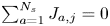 $\sum _{a=1}^{N_s} J_{a,j} = 0$. In (3.8),
 $D$ is the mass diffusivity, a material property discussed in § 3.2 and appendix A.5.
Equation (3.3) states the Navier–Stokes equations for conservation of momentum in each of the three coordinate directions. The deviatoric, symmetric viscous stress tensor is
 \begin{equation} \sigma_{ij} = 2 \mu \left( S_{ij} - \frac{1}{3} \frac{ \partial u_k}{ \partial x_k} \delta_{ij} \right), \end{equation}
where
 \begin{equation} S_{ij}= \frac{ 1}{2} \left( \frac{ \partial u_i}{ \partial x_j} + \frac{ \partial u_j}{ \partial x_i} \right) \end{equation}
is the rate of strain tensor and  $\mu$ is the viscosity, a material property discussed in § 3.2, appendix A.5 and the supplementary material. Note that momentum transport is assumed to be due to ions only; the momentum of free electrons is not considered (nor is their mass).
Equation (3.4) is the equation for conservation of energy of the ions. The ion energy per unit volume consists of internal and kinetic energy components; it is
 \begin{equation} E_n= \rho \left( \mathcal{E}_n + \tfrac{1}{2} u_i u_i \right), \end{equation}
where  $\mathcal {E}_n$ is the specific ion internal energy (i.e. the internal energy stored in the ions per unit fluid mass), computed from the EOSs. The right-hand side of (3.4) includes a term involving
 $J_{a,j}$ that is required for flows with multispecies diffusion (Cook Reference Cook2009). The species-
 $a$ specific ion enthalpy
 $h_{n,a}$ is discussed further in appendix A.4. The heat flux vector for ion thermal conduction is
 \begin{equation} q_{n,j}= - \kappa_n \frac{ \partial T_n}{\partial x_j}, \end{equation}
where  $T_n$ is the ion temperature and
 $\kappa _n$ is the ion thermal conductivity, a material property discussed in § 3.2 and appendix A.5.
Equation (3.5) is the equation for conservation of energy of the free electrons. The electron energy per unit volume is  $E_e = \rho \mathcal {E}_e$, where
 $\mathcal {E}_e$ is the specific electron internal energy (i.e. the internal energy stored in the free electrons per unit fluid mass), computed from the EOSs. The heat flux vector for electron thermal conduction is
 \begin{equation} q_{e,j}= -\kappa_e \frac{ \partial T_e}{\partial x_j}, \end{equation}
where  $T_e$ is the electron temperature and
 $\kappa _e$ is the electron thermal conductivity, a material property discussed in § 3.2 and appendix A.6. The ion–electron energy coupling term is
 \begin{equation} \dot{Q}_{n e}= \rho c_{v,e} K_{n e} \left(T_n - T_e \right), \end{equation}
where  $K_{n e}$ is a coupling coefficient calculated from the approximate model of Brysk (Reference Brysk1974, (35)), which was derived by considering ion–electron collisions in an ideal gas including Fermi–Dirac electron statistics. In (3.14),
 $c_{v,e} = ({\partial \mathcal {E}_e / \partial T_e})_{\rho }$ is the specific electron heat capacity at constant volume, a material property calculated from the EOSs. Note that the opposite of
 $\dot {Q}_{n e}$ is added to (3.4).
Equation (3.6) is the radiation transport equation for conservation of radiation energy. The radiation energy per unit volume  $E_r$ is treated as grey, meaning that it represents an integral over energies at each photon frequency. It is related to the radiation temperature
 $T_r$ through
 \begin{equation} E_r= \frac{4 \sigma_o T_r^4}{c_o}. \end{equation}
Equation (3.6) is derived from a more complete description of radiative transfer (Castor Reference Castor2004, (4.24)) by making a diffusion approximation, i.e. that photon mean free paths are small relative to other length scales (Brunner Reference Brunner2002; Castor Reference Castor2004). The flux limiter is
 \begin{equation} \varUpsilon = \left( 3 + \frac{ 1}{\varUpsilon_o \rho \varkappa_r E_r} \left[ \frac{ \partial E_r}{ \partial x_k} \frac{ \partial E_r}{ \partial x_k} \right]^{1/2} \right)^{-1}, \end{equation}
which is called a sum flux limiter per Olson, Auer & Hall (Reference Olson, Auer and Hall2000, (9)) and Castor (Reference Castor2004, (11.76)). The constant  $\varUpsilon _o$, which may be viewed as an additional tuning parameter, is set to unity here. The flux limiter serves to prevent unphysical wave propagation velocities, as explained by Olson et al. (Reference Olson, Auer and Hall2000) and Castor (Reference Castor2004). See Castor (Reference Castor2004) for a comprehensive discussion of radiation transport, and see Levermore & Pomraning (Reference Levermore and Pomraning1981) and Pomraning (Reference Pomraning1982) for foundational work on flux limiters in radiation diffusion equations. We assume that radiation pressure is negligible, which is a reasonable assumption at the moderate densities and the not extremely high (i.e. sub-keV) temperatures considered here.
As mentioned in § 2, a principal goal of the present study is to enable comparisons between the HED flows of the Reshock Campaign and their non-HED analogues. It is instructive to compare (3.1)–(3.6) to the governing equations in the simulations of Hill et al. (Reference Hill, Pantano and Pullin2006) or those of Tritschler et al. (Reference Tritschler, Olson, Lele, Hickel, Hu and Adams2014). Excepting any convolution with LES filtering operators, the underlying equations for conservation of total mass, species mass and momentum in these non-HED computational studies are identical to those in the present study. Conversely, the HED case involves three distinct, coupled equations for conservation of energy – including distinct terms for ion and electron thermal conduction – while the non-HED cases each involve a single equation for conservation of energy. Section 5 investigates the role of electron thermal conduction in detail.
3.2. Material properties
This section briefly summarizes the models for properties of the three pure materials  $\mathbb {M}_H$,
 $\mathbb {M}_L$ and
 $\mathbb {M}_R$ (each treated as a single species) and of multispecies mixtures. Appendix A provides detailed elaboration on all of the models described in this section, including key EOS and opacity model parameters needed to reproduce all the simulations in the present study.
Equations (3.1)–(3.6) and the associated models are based on the foundational assumption that the pressure  $p$ and specific internal energy
 $\mathcal {E}_l$ of a material can be separated into contributions due to ions and free electrons (Zel'dovich & Raizer Reference Zel'dovich and Raizer2002; Ramshaw & Cook Reference Ramshaw and Cook2014). For a single species, the total pressure
 $p$ is expressed as the sum of the ion (partial) pressure
 $p_{n}$ and the electron (partial) pressure
 $p_{e}$
 \begin{equation} p = p_{n} + p_{e}. \end{equation}
Similarly, the specific total internal energy  $\mathcal {E}_l$ is
 \begin{equation} \mathcal{E}_l= \mathcal{E}_{n} + \mathcal{E}_{e}. \end{equation}
Ion motion is associated with the ion temperature  $T_n$, and free-electron motion with the electron temperature
 $T_e$. For the present study and for a single species, pressures and specific internal energies are expressed in terms of densities and temperatures using the quotidian equation-of-state (QEOS) model of More et al. (Reference More, Warren, Young and Zimmerman1988). The degree of ionization
 $Z^{*}$, defined as the number of free electrons per nucleus, is given by an analytic fit (More Reference More1991) to numerical results from Thomas–Fermi theory (Feynman, Metropolis & Teller Reference Feynman, Metropolis and Teller1949). The Rosseland and Planck mean opacities,
 $\varkappa _r$ and
 $\varkappa _p$, respectively, are modelled using an analytic form suggested by Atzeni & Meyer-ter-Vehn (Reference Atzeni and Meyer-ter-Vehn2004).
Multispecies mixtures within a computational zone are treated using a free-electron- biased thermodynamic equilibration framework (Ramshaw & Cook Reference Ramshaw and Cook2014), which defines an effective multispecies EOS in terms of the single-species EOSs. Degrees of ionization and opacities of multispecies mixtures are defined as explicit functions of the single-species quantities.
The coefficients for transport processes involving ions – the mass diffusivity  $D$, viscosity
 $\mu$ and ion thermal conductivity
 $\kappa _n$ – are derived from kinetic theory (Hirschfelder, Curtiss & Bird Reference Hirschfelder, Curtiss and Bird1954; Chapman & Cowling Reference Chapman and Cowling1970). The relevant collision integrals are calculated using a screened Coulomb potential to treat ion–ion binary collisions (Stanton & Murillo Reference Stanton and Murillo2016). The electron thermal conductivity
 $\kappa _e$ is derived from an analysis (Lee & More Reference Lee and More1984) of the Boltzmann equation for the electron distribution function and from subsequent work (Managan Reference Managan2015).
3.3. Numerical methods
Approximate solutions to (3.1)–(3.6) were obtained using the radiation hydrodynamics code Ares. The code implements an arbitrary Lagrangian–Eulerian (ALE) scheme based originally on work by Sharp & Barton (Reference Sharp and Barton1981). Each time step consists of a Lagrangian phase, in which the mesh moves with the flow, and a remap (or advection) phase, in which (i) the mesh is relaxed (without altering the flow field) towards its previous state by a relative amount  $\mathcal {J} \in [0,1]$ and (ii) the flow field is interpolated onto the new mesh. For the present study, we always ran Ares in the
 $\mathcal {J}=1$ full remap mode. This yielded simulations that were effectively Eulerian only, with no net Lagrangian distortion of the mesh. When running in this mode and except near flow discontinuities, the spatial discretization scheme is second-order accurate. Explicit time integration is performed using a second-order predictor–corrector scheme (Darlington, McAbee & Rodrigue Reference Darlington, McAbee and Rodrigue2001). Artificial viscosity (originally proposed by von Neumann & Richtmyer (Reference von Neumann and Richtmyer1950) and discussed in detail by Richtmyer & Morton (Reference Richtmyer and Morton1967)) is added to maintain numerical stability near shocks. In the present study, the artificial viscosity scheme incorporates a monotonic limiter, based approximately on the van-Leer-type flux limiters (van Leer Reference van Leer1979) used widely in approximate Riemann solvers (Toro Reference Toro2009). Ion thermal conduction, electron thermal conduction and radiation diffusion are treated using a first-order implicit-time operator-splitting framework.
Ares incorporates an AMR capability via the SAMRAI library (Wissink et al. Reference Wissink, Hornung, Kohn, Smith and Elliott2001). In the present study, this capability granted major reductions in computational cost. Indeed, throughout all the simulations, the regions of the domain featuring significant variation in quantities like the species mass fractions or the total pressure comprised only small fractions of the total length  $W$ in figure 1. Beginning with a uniform Cartesian level-0 mesh with cubic zones of edge length
 $\Delta x_{0}$, we allowed for two levels of AMR. On the level-1 and level-2 meshes, the edge lengths were
 $\Delta x_{1}= \Delta x_{0}/3$ and
 $\Delta x_{2}= \Delta x_{1}/3= \Delta x_{0}/9$, respectively. See table 1 for additional specification of the simulation meshes. Refinement criteria were designed such that the maximum-resolution level was active at or near any sharp gradient in density or electron pressure, any non-negligible
 $\mathbb {M}_H$–
 $\mathbb {M}_L$ mixing and both the
 $x=0$ and
 $x=W$ edges of the domain (where the main shock and reshock formed at early time).
The simulations were monitored carefully to ensure robustness of all critical algorithms. Frequent checks were made to ensure that maximal mesh refinement was maintained, with large buffers, around all flow features of interest at all times. Matrix inversion operations, particularly those involved in calculating ion and electron thermal conduction and radiation diffusion, were watched. Excellent convergence behaviour was observed in all cases. Iterative methods used to equilibrate multispecies mixtures within zones, as discussed in § 3.2 and appendix A.4, were also audited. Again, excellent convergence behaviour was observed in all cases.
For detailed analysis of the numerical performance of Ares, including comparisons between Ares and a higher-order Eulerian code, see Olson & Greenough (Reference Olson and Greenough2014). Numerical properties of the Ares solver are also discussed by Morgan & Greenough (Reference Morgan and Greenough2016), Thornber et al. (Reference Thornber2017) and Morgan et al. (Reference Morgan, Olson, Black and McFarland2018). All four of those works applied Ares to problems with instability growth and multispecies mixing. Bowers & Wilson (Reference Bowers and Wilson1991) and Castor (Reference Castor2004) are general references on the design of radiation hydrodynamics codes. We reiterate that our present focus is on the physics of HED shock-induced mixing, not on numerical analysis of the Ares solver nor on implementation of algorithms. Thus, for example, we do not attempt to quantify the numerical dissipation of the Ares ALE scheme (as do Olson & Greenough (Reference Olson and Greenough2014)). Instead, we draw physical conclusions based on simulation-derived quantities of interest, while scrutinizing the sensitivity of those quantities to mesh resolution.
3.4. Warm initially stable interface approximation
The EOS model used in the present study describes matter in the solid, liquid, gas or plasma states; see appendix A.1. In the NIF experiments, the CHI, CRF and PAI materials were all initially solids, before they were driven into the HED regime. However, we do not expect that phenomena unique to the solid state, such as elastic deformation or the crushing of voids in the porous foam, had significant roles in post-shock CHI–CRF instability growth and mixing.
Accordingly, to simplify our simulations and enable clearer comparisons with non-HED reshock studies, we opt to altogether bypass the solid-state thermodynamic regimes of the materials. Two choices are made in our simulations. First, the entire domain is initialized with  $T_n= T_e = 1\ \textrm {eV}$, sufficiently above the boiling temperatures of
 $\mathbb {M}_H$,
 $\mathbb {M}_L$ and
 $\mathbb {M}_R$. At these temperatures and at the densities stated in § 2, the total pressures in the three materials are different, e.g. by approximately 0.22 Mbar for
 $\mathbb {M}_H$ and
 $\mathbb {M}_L$. Consequently, if no other action were taken, pressure imbalances would cause displacement of the interfaces before arrival of the shock waves. Therefore, second, the following constraints are imposed: at each time step, local mixture-equilibrated pressures are calculated and, if either the electron pressure
 $p_e$ or the ion pressure
 $p_n$ is less than 0.4 Mbar, then the pressures used in the discretized forms of (3.3)–(3.5) are set to zero. These constraints keep the
 $\mathbb {M}_H$–
 $\mathbb {M}_L$ and
 $\mathbb {M}_L$–
 $\mathbb {M}_R$ interfaces stable until they are impacted by the first shock and reshock, respectively, which exhibit pressures well above the 0.4 Mbar threshold. The pressure-based constraints are removed after both interfaces are shocked, i.e. after both shocks have transmitted into the
 $\mathbb {M}_L$ region.
We call this scheme the warm initially stable interface (WISI) approximation. It considerably simplifies our analysis by ensuring that all materials are always in a state credibly described by the equations of fluid mechanics. Also, it nearly eliminates thermal conduction at the interfaces before arrival of the shock waves, thereby ensuring that, at a given resolution, the pre-shock interfaces in the baseline simulation and the CPV are nearly identical. (Note that the WISI approximation does not prevent mass diffusion, which is associated with some energy transfer at the interfaces via (3.4). However, this effect is minor. For example, simulated temperatures at the edges of the  $\mathbb {M}_H$–
 $\mathbb {M}_L$ interface at 10 ns deviate from the initial temperature by
 ${<}0.002\ \textrm {eV}$.) In preliminary calculations, we observed little sensitivity of shock trajectories to the precise values, within reasonable bounds, of the initial temperature and the pressure threshold used in the WISI approximation.
3.5. Statistical averaging
Much of the analysis in §§ 4 and 5 is based on statistical averaging of flow variables in the mixing layers. Let  $\phi$ be any flow variable, which in general is a function of
 $x$,
 $y$,
 $z$ and
 $t$. Following the conventions in Sagaut & Cambon (Reference Sagaut and Cambon2008), Chassaing et al. (Reference Chassaing, Antonia, Anselmet, Joly and Sarkar2010) and Gatski & Bonnet (Reference Gatski and Bonnet2013), let
 $\overline {\phi }$ be the Reynolds average,
 $\phi '$ the Reynolds fluctuation,
 $\widetilde {\phi }= \overline { \rho \phi }/\bar {\rho }$ the Favre average and
 $\phi ''$ the Favre fluctuation, with
 $\phi \equiv \overline { \phi }+ \phi '$ and
 $\phi \equiv \widetilde { \phi }+ \phi ''$. The Reynolds average
 $\overline {(\cdot )}$ is defined as a mean over an ensemble of flows. However, here, spatial averaging over the
 $y$ and
 $z$ spanwise directions is employed as a surrogate for ensemble averaging, as is commonly done in computational studies of mixing layers
 \begin{equation} \overline{\phi} = \overline{\phi}(x, t) = \frac{1}{L^2} \int_{0}^{L} \int_{0}^{L} \phi( x, y, z, t)\,{\textrm{d}y}\,\textrm{d}z. \end{equation}
The supplementary material provides additional discussion of averaging operators.
Consider the  $\mathbb {M}_H$–
 $\mathbb {M}_L$ mixing region at time
 $t$. Call the
 $-x$ edge of the mixing region (closest to pure-
 $\mathbb {M}_H$ plasma) the bubble front
 $x_b( t)$, and call the
 $+x$ edge of the mixing region (closest to pure-
 $\mathbb {M}_L$ plasma) the spike front
 $x_s( t)$. These terms are motivated by conventions for RM or RT instability growth: a bubble is low-density fluid penetrating into high-density fluid, and a spike is high-density fluid penetrating into low-density fluid (Atzeni & Meyer-ter-Vehn Reference Atzeni and Meyer-ter-Vehn2004). Then, the total mixing-layer width is
 \begin{equation} \mathcal{W}(t)= x_s( t)- x_b( t). \end{equation}
For any flow variable  $\phi$, the mixing-layer average of
 $\phi$ is
 \begin{equation} \langle\!\langle {\phi} \rangle\!\rangle ( t) \equiv \frac{1}{\mathcal{W}( t)} \int_{x_b}^{x_s} \overline{\phi}( x, t)\, {\textrm{d}\kern0.7pt x}. \end{equation}
The mixing-layer integral of  $\phi$ is
 \begin{equation} \lfloor {\phi} \rfloor( t) \equiv \frac{1}{W} \int_{x_b}^{x_s} \overline{\phi}( x, t) \,{\textrm{d}\kern0.7pt x}, \end{equation}
where  $W$ is the total
 $x$-extent of the domain per figure 1. Here,
 $\lfloor {\cdot } \rfloor$ should not be mistaken for the mathematical floor function. The distinction between
 $\langle\!\langle {\phi } \rangle\!\rangle$ and
 $\lfloor {\phi } \rfloor$ is subtle but important. If
 $\phi$ is equal to a constant
 $\phi _o$, then
 $\langle\!\langle {\phi } \rangle\!\rangle$ is identically
 $\phi _o$, while
 $\lfloor {\phi } \rfloor = \phi _o \mathcal {W} / W$ is proportional to the total mixing-layer width
 $\mathcal {W}$. Both
 $\langle\!\langle {\phi } \rangle\!\rangle$ and
 $\lfloor {\phi } \rfloor$ have the same units as
 $\phi$. In general, the
 $\lfloor {\cdot } \rfloor$ operator is better suited to extensive properties that might be expected to increase with mixing-layer size, while the
 $\langle\!\langle {\cdot } \rangle\!\rangle$ operator is better suited to intensive properties. Note that the normalizing constant
 $W$ is included in the definition of
 $\lfloor {\cdot } \rfloor$ principally to simplify dimensional analysis. We choose to use
 $W$ because it is an easily measured parameter in the NIF experiments and is unlikely to change in future versions of the present simulations. However, alternate choices for the constant could be made with no impact on our conclusions.
The following method is used to calculate  $x_b$ and
 $x_s$ at a given
 $t$. First, compute the Reynolds-averaged mass fraction
 $\overline {Y}_L( x)$ of the light material
 $\mathbb {M}_L$:
 $\overline {Y}_L$ is zero for small
 $x$, rises to one after traversing the
 $\mathbb {M}_H$–
 $\mathbb {M}_L$ mixing region, and drops to zero again after traversing the
 $\mathbb {M}_L$–
 $\mathbb {M}_R$ interface. Importantly, in the present simulations (and in the experiments), the main ablator never mixes completely through the foam, i.e. there is always some region of pure foam located between the main ablator and the reshock ablator. Let
 $x_b$ be the first point, starting in the pure
 $\mathbb {M}_H$ plasma and scanning in the
 $+x$ direction, for which
 $\overline {Y}_L= Y^{*}$. Let
 $x_s$ be the first point, starting in the pure
 $\mathbb {M}_L$ plasma and scanning in the
 $-x$ direction, for which
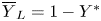 $\overline {Y}_L= 1 - Y^{*}$. Here,
 $Y^{*}$ is a mass-fraction threshold, taken to be
 $0.01$ in all cases, i.e. a
 $1\,\%\text {--}99\,\%$ criterion defines the mixing-layer boundaries. The choice for
 $Y^{*}$ is somewhat arbitrary. Setting
 $Y^{*}=0.01$ gave a reasonable correspondence to experimentally determined bubble and spike fronts from the X-ray radiographs. Indeed, a relatively small amount of
 $\mathbb {M}_H$–
 $\mathbb {M}_L$ mixing led to changes in X-ray transmission that appeared as discernible mixing-layer edges in the NIF images (Huntington et al. Reference Huntington, Raman, Nagel, MacLaren, Baumann, Bender, Prisbrey, Simmons, Wang and Zhou2020). Importantly, we do not see evidence that any of the qualitative results in §§ 4 and 5 are sensitive to the exact value of
 $Y^{*}$, provided that it is small. Plots and further discussion of
 $\overline {Y}_L$ are included in § 4.2.
3.6. Tuning to experimental data
We next turn our attention to methodology for constraining the computational model to available experimental data from the NIF. These data are incorporated into two critical elements of the simulations: (i) the radiation temperature boundary conditions, which drive the formation of the main shock and reshock; and (ii) the initial perturbation at the main-ablator–foam interface, which seeds instability growth.
3.6.1. Radiation temperature boundary conditions
Time-dependent radiation temperature boundary conditions, also called sources, are applied to the  $x=0$ and
 $x=W$ surfaces of the domain as depicted in figure 1. The radiation temperature is set in the centres of ghost zones located just outside the edges of the domain. The
 $x=0$ boundary condition
 $T_{r,{main}}(t)$ is the main-drive source, and the
 $x=W$ boundary condition
 $T_{r,{reshock}}(t)$ is the reshock-drive source. The sources approximately capture the effects of the X-ray baths inside the two laser-irradiated halfraums in the NIF experiments. In this work, we do not attempt to derive the sources from detailed models of the halfraums. Instead, we interpret
 $T_{r,{main}}$ and
 $T_{r,{reshock}}$ as adjustable functions of
 $t$, and we tune them to achieve main-shock and reshock trajectories that are consistent with experimental data from the Reshock Campaign. For the tuning procedure, shock positions over time are determined by tracking characteristics (Anderson Reference Anderson2003) in a simplified one-dimensional (1-D) version of the finest-resolution 3-D baseline simulation per table 1. Appendix B provides justification for the use of a 1-D simulation in this way. The tuning procedure is extremely important. It serves to calibrate the computational model – including the diffusive treatment of radiation transport; the material EOSs, degrees of ionization and opacities; and the WISI approximation for domain initialization – to measurable quantities from the NIF. The radiation transport equation (3.6) is especially crucial for modelling early-time shock formation near the
 $x=0$ and
 $x=W$ boundaries. In a future study, if any substantial changes were made to the model as outlined in §§ 3.1–3.4, then the tuning procedure would need to be repeated.
The following functional form is used for the two sources:
 \begin{equation} T_r(t)= \sum_{ \iota= 1}^{3} B_{1,\iota} \left(\frac{t}{B_{2,\iota}}\right)^{B_{3,\iota}} \exp \left( -\frac{t}{B_{2,\iota}} \right). \end{equation}
This form allows for replication of typical qualitative features of radiation temperature histories in NIF halfraums, i.e. a sharp initial peak in  $T_r$ followed by intermediate-time stabilization and late-time decay. See, for example, figure 3(b) of Nagel et al. (Reference Nagel2017). The coefficients
 $B_{1,1}, B_{2,1}, \ldots$ are defined separately for
 $T_{r,{main}}$ and
 $T_{r,{reshock}}$.
To set the coefficients, shock trajectories are compared to experimental data from three different NIF shots. The first of these involved a standard Reshock Campaign target, with two halfraums, as described in § 2. Using the techniques of Nagel et al. (Reference Nagel2017) and Huntington et al. (Reference Huntington, Raman, Nagel, MacLaren, Baumann, Bender, Prisbrey, Simmons, Wang and Zhou2020), an X-ray radiograph was taken at a time when both the main shock and reshock were clearly visible in the foam region. Hence, this shot gave measurements of the two shock positions at a known time. The second NIF shot used a single-halfraum target consisting of only the main ablator region placed next to a block of quartz. The velocity interferometer system for any reflector (VISAR) optical diagnostic (Celliers et al. Reference Celliers, Bradley, Collins, Hicks, Boehly and Armstrong2004) was used to measure shock speed in the quartz over time. In particular, a measurement was made of the time for the shock to traverse the  $550\ \mathrm {\mu }\textrm {m}$ main ablator region, called the main-shock breakout time. The third NIF shot used a single-halfraum target consisting of only the reshock ablator region placed next to a thin block of aluminium followed by a larger block of quartz. The VISAR diagnostic was used again to measure shock speed in the quartz over time. From this shot, it was possible (using simulations not detailed here) to infer the time for the shock to traverse the
 $150\ \mathrm {\mu }\textrm {m}$ reshock ablator region, called the reshock breakout time. Quartz is a common material used when making VISAR measurements in HED experiments, because strong shocks in quartz are highly reflective. A full discussion of the VISAR technique, and the NIF shots in which it was implemented, is beyond our scope. Celliers et al. (Reference Celliers, Bradley, Collins, Hicks, Boehly and Armstrong2004) discuss the technique in detail.
Figure 2 plots the simulated main-shock and reshock trajectories when using the tuned sources, along with the experimental data from the three NIF shots described in the previous paragraph. Figure 3 plots the tuned sources  $T_{r,{main}}$ and
 $T_{r,{reshock}}$. Table 8 gives the corresponding coefficient values.
Simulated main-shock and reshock trajectories (Sim) and comparison with experimental data (Exp), with  $x$ the position in the coordinate system of figure 1 and
 $t$ the time. The simulated trajectories are from a 1-D version of the finest-resolution 3-D baseline simulation. Also plotted is the mixing-layer centre-plane position, defined by (4.3), from the finest-resolution 3-D baseline simulation. Horizontal and vertical error bars on the experimental data are shown only when larger than the symbol sizes. Appendix B elaborates on the use of 1-D calculations for analysing shock trajectories. The experimental data are tabulated in the supplementary material.


3.6.2. Interface initial perturbation
A multimode initial perturbation is applied to the  $\mathbb {M}_H$–
 $\mathbb {M}_L$ interface as schematically depicted in figure 1. Specifically, the
 $t=0$ material compositions of zones in the vicinity of the
 $x=W_H$ plane are defined using a multistep procedure described in this section and in appendix D. The procedure yields a computational representation that meets several important criteria: (i) it captures key features of the physical perturbations in the experiments; (ii) it is periodic in both the
 $y$ and
 $z$ directions with period
 $L$; (iii) it is based on spectral modes whose wavelengths are reasonable compared to the zone size; and (iv) it is based on a smooth analytic functional form that is formally independent of the mesh. Our discussion uses the Fourier analysis conventions summarized in appendix E and based on Press et al. (Reference Press, Teukolsky, Vetterling and Flannery1992).
First define the total perturbation function
 \begin{equation} \delta_x ( y, z ) = \delta_x^{{\dagger}} (y) + \delta_x^{*} (y,z) \end{equation}
in the coordinate system of figure 1. It consists of two components, the principal-perturbation function  $\delta _x^{{\dagger} }$ and the noise-perturbation function
 $\delta _x^{*}$. The principal-perturbation function is only a function of
 $y$. When visualized as a 2-D surface, it appears as a 1-D curve extruded into the
 $z$ direction. It approximately corresponds to the multimode profile specified in the experimental NIF target designs. In each target, a perturbation was machined – via extruded cuts along one coordinate direction – onto one surface of the main ablator, prior to assembly with the foam and other components. The nominal profile was the same across all the experiments. No perturbation was machined onto the foam, i.e. the extruded cuts in the main ablator were not mirrored by cuts in the foam. The nominal profile only contains spectral modes with wavelengths ranging from
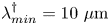 $\lambda _{{min}}^{{\dagger} } = 10\ \mathrm {\mu }\textrm {m}$ to
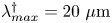 $\lambda _{{max}}^{{\dagger} } = 20\ \mathrm {\mu }\textrm {m}$, and its power spectral density has a top-hat shape.
The noise-perturbation function is a function of both  $y$ and
 $z$. It accounts for various irregularities that might be expected in the NIF targets, such as machining imperfections, foam heterogeneity, interfacial voids and local crushing of the foam as it is pressed against the rippled main-ablator surface. While these irregularities have not been exhaustively studied, their characteristic modes are expected to be of higher frequency and lower amplitude than those in the nominal multimode profile. For example, characteristic pore sizes in the foam have been observed to be sub-
 $\mathrm {\mu }\textrm {m}$ (Huntington et al. Reference Huntington, Raman, Nagel, MacLaren, Baumann, Bender, Prisbrey, Simmons, Wang and Zhou2020). In the present study, we choose to construct
 $\delta _x^{*}$ such that it only contains spectral modes with wavelengths ranging from
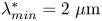 $\lambda _{{min}}^{*} = 2\ \mathrm {\mu }\textrm {m}$ (slightly larger than the zone edge length
 $\Delta x_{2}$ on the finest AMR level of the coarsest mesh per table 1) to
 $\lambda _{{max}}^{*} = 5\ \mathrm {\mu }\textrm {m}$ and such that its power spectral density has a top-hat shape. The values for
 $\lambda _{{min}}^{*}$ and
 $\lambda _{{max}}^{*}$ should be understood as modelling choices; they are not explicit in the NIF target designs, in contrast to
 $\lambda _{{min}}^{{\dagger} }$ and
 $\lambda _{{max}}^{{\dagger} }$. Note that
 $\delta _x^{*}$ has an important role in the simulations, because it contributes to symmetry breaking and three-dimensionality in the evolving flow.
Appendix D details the procedures for constructing  $\delta _x^{{\dagger} }$ and
 $\delta _x^{*}$. The latter procedure is based on the approach of Thornber et al. (Reference Thornber2017). The functions
 $\delta _x^{{\dagger} }$ and
 $\delta _x^{*}$ are designed such that their amplitudes – or, more precisely, the standard deviations
 $S^{{\dagger} }$ and
 $S^{*}$ of suitably large numbers of samples of
 $\delta _x^{{\dagger} }$ and
 $\delta _x^{*}$, respectively – are easily adjustable. Neither function depends on the mesh resolution.
The total perturbation function  $\delta _x$ is cast onto the simulation domain via specification of zonal mass fractions near the
 $x=W_H$ plane. Each of these zones contains at most two species,
 $\mathbb {M}_H$ and
 $\mathbb {M}_L$. Define the interface smoothing function by
 \begin{equation} \zeta( s)= \frac{1}{2} \left[ 1 + \mathrm{erf}\left( \frac{ s}{\zeta_o} \right) \right], \end{equation}
where  $\zeta _o$ is the interface smoothing length and
 $\mathrm {erf}$ is the error function. The initial mass fraction of the light material in the interfacial zones is calculated according to
 \begin{equation} Y_L( x, y, z)= \zeta \left( x- [ W_H + \delta_x( y, z)] \right). \end{equation}
The initial mass fraction of the heavy material is  $Y_H= 1-Y_L$. Initial densities and specific internal energies of the mixtures in the interfacial zones are calculated in the natural way from those of the pure species
 $\mathbb {M}_H$ and
 $\mathbb {M}_L$. In this work,
 $\zeta _o \approx 1.076\ \mathrm {\mu }\text {m}$, a somewhat arbitrary choice based on characteristic amplitudes in the experimental multimode profile. (Instead,
 $\zeta _o$ could be interpreted as an additional tuning parameter, but we choose not to do so.) Notice that the interface smoothing function does not depend on the mesh resolution. Thus, the computational representation of the interfacial region converges under mesh refinement to the analytic form given by (3.25) and (3.26).
It remains to discuss how the amplitudes of the principal- and noise-perturbation functions are set. The standard deviations  $S^{{\dagger} }$ and
 $S^{*}$ are adjusted until the computational mixing-layer width
 $\mathcal {W}(t)$ from (3.20) agrees with experimental measurements at six different times. The experimental data
 $\{\mathcal {W}_{{exp},i}\}$ were acquired, using the technique introduced by Huntington et al. (Reference Huntington, Raman, Nagel, MacLaren, Baumann, Bender, Prisbrey, Simmons, Wang and Zhou2020), from X-ray radiographs from six NIF shots with nominally identical targets. One data point was acquired per shot. For this tuning procedure, which involves multiple full-scale 3-D simulations, we use the coarsest-resolution mesh described in table 1. Ultimately, setting
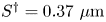 $S^{{\dagger} } = 0.37\ \mathrm {\mu }\textrm {m}$ and
 $S^{*} = 0.074\ \mathrm {\mu }\textrm {m}$ gives reasonable experimental–computational agreement, and these values for
 $S^{{\dagger} }$ and
 $S^{*}$ are held fixed across all the simulations described in this paper. For comparison, the standard deviation of the experimental multimode profile was
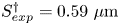 $S^{{\dagger} }_{exp} = 0.59\ \mathrm {\mu }\textrm {m}$. The difference between
 $S^{{\dagger} }$ and
 $S^{{\dagger} }_{exp}$ reflects the many modelling simplifications described in this section. Plots and further analysis of
 $\mathcal {W}(t)$ from the tuned simulations, including comparison with
 $\{\mathcal {W}_{{exp},i}\}$, are included in § 4.1.
Figure 4 provides visualizations of the perturbation construction procedure. Shown are the principal-perturbation function  $\delta _x^{{\dagger} }$ in figure 4(a) and representative 1-D slices through the noise-perturbation function
 $\delta _x^{*}$ and the total perturbation function
 $\delta _x$ in figures 4(b) and 4(c), respectively. The ordinate-axis limits in figure 4(b) are different from those in figures 4(a) and 4(c), reflecting the fact that
 $S^{{\dagger} }/S^{*} = 5$. Per the definitions in appendix E, figure 4(d) plots the
 $\delta _x$ radial power spectral density (RPSD), which exhibits two plateaus: one corresponds to the principal-perturbation minimum and maximum wavelengths (10 and 20
 $\mathrm {\mu }\textrm {m}$, respectively), and the other corresponds to the noise-perturbation minimum and maximum wavelengths (2 and
 $5\ \mathrm {\mu }\textrm {m}$, respectively). By design, there is negligible spectral power at the intermediate wavelengths between 5 and
 $10 \ \mathrm {\mu }\textrm {m}$. Figure 4(e) plots the interface smoothing function
 $\zeta$. Figure 4(f) plots, for each of the three baseline simulations, the RPSD of the heavy-material mass fraction
 $Y_H$ at the interface centre-plane. Thus, the RPSDs in figure 4(f) – unlike those in figure 4(d) – include the effects of encoding
 $\delta _x$ onto the discretized simulation domains. Good convergence behaviour is seen in the plateaus of the RPSDs, as expected. The spectral power present at the intermediate wavelengths from 5 to
 $10\ \mathrm {\mu }\textrm {m}$ results from the nonlinearity in
 $\zeta$. Indeed, we confirmed that the intermediate-wavelength spectral power diminishes – compared to the spectral power on the plateaus – as the interface smoothing length
 $\zeta _o$ increases; increasing
 $\zeta _o$ widens the interval, centred at
 $s=0$, over which
 $\zeta (s)$ is approximately linear.
Visualizations of the tuned  $\mathbb {M}_H$–
 $\mathbb {M}_L$ interface initial perturbation and related quantities: (a) plots the 1-D principal-perturbation function
 $\delta _x^{{\dagger} }$; (b) plots the 1-D slice at
 $z=0$ through the 2-D noise-perturbation function
 $\delta _x^{*}$; (c) plots the 1-D slice at
 $z=0$ through the 2-D total perturbation function
 $\delta _x$, along with
 $\delta _x^{{\dagger} }$ for comparison; (d) plots (Num) the numerically calculated RPSD of
 $\delta _x$ using (E9), along with (Fid) analytically calculated fiducial RPSD values of
 $\delta _x^{{\dagger} }$ and
 $\delta _x^{*}$ using Parseval's theorem; (e) plots the interface smoothing function
 $\zeta$ of (3.25); and (f) plots the RPSD of the initial
 $\mathbb {M}_H$ mass fraction
 $Y_H$ at the centre-plane
 $x=x_c$ in the three baseline simulations. Equation (4.3) defines the coordinate
 $x_c$. In (d,f), the abscissa is the spectroscopic wavevector magnitude. In (f), the legend states
 $\mathcal {N}_{yz,2}$ as defined in the caption of table 1. See appendix D for full specifications of
 $\delta _x^{{\dagger} }$ and
 $\delta _x^{*}$, and see appendix E for additional description of Fourier analysis conventions.

4. Results and analysis: baseline simulations
This section discusses results from the three baseline simulations summarized in table 1. When comparing the three cases, we often reference them by  $\mathcal {N}_{yz,2}$, the number of zones counted linearly along either the
 $y$ or
 $z$ spanwise directions on the finest AMR level. As noted in § 3.3, this level of refinement is maintained at all times wherever there is multimaterial mixing (among other criteria). For instance, in the finest-resolution case, a planar cross-section through the centre of the mixing layer consists of
 $360 \times 360$ zones.
4.1. Phases of mixing-layer growth
Figure 5 plots time histories of the mixing-layer width  $\mathcal {W}$ as defined by (3.20) using a
 $1\,\%\text {--}99\,\%$ mass-fraction criterion. At
 ${\sim }11\ \textrm {ns}$, the main shock arrives at the
 $\mathbb {M}_H$–
 $\mathbb {M}_L$ interface, initiating perturbation growth via the RM instability mechanism. At
 ${\sim }31\ \textrm {ns}$, the reshock arrives at and compresses the developing mixing layer. At
 ${\sim }33\ \textrm {ns}$, rapid post-reshock growth begins. The growth rate decreases at later times, with the maximum width reached at
 ${\sim }45\ \textrm {ns}$. Finally, from
 ${\sim }45$ to
 $50\ \textrm {ns}$, a weak compression event occurs. It corresponds to the impact of the reflection (moving in the
 $-x$ direction) of the main shock off the reshock ablator
 $\mathbb {M}_R$, which was initially accelerated towards the
 $\mathbb {M}_H$–
 $\mathbb {M}_L$ interface. This late-time event is analysed further in § 4.3.
Evolution of the mixing-layer width  $\mathcal {W}$ from (3.20) in the baseline simulations (Sim), along with NIF experimental measurements (Exp). For the simulations, the legend states
 $\mathcal {N}_{yz,2}$ as defined in the caption of table 1. The experimental data are tabulated and further discussed in the supplementary material.

Figure 5 also includes six experimental measurements of the mixing-layer width from NIF shots. As explained in § 3.6.2, the coarsest-resolution baseline simulation was tuned to these data  $\{\mathcal {W}_{{exp},i}\}$ by adjusting the perturbation-component standard deviations
 $S^{{\dagger} }$ and
 $S^{*}$. Once fixed, the same parameters were used in all simulations. Accordingly,
 $\mathcal {W}$ agrees well with
 $\{\mathcal {W}_{{exp},i}\}$ in the 180-zone case. The higher-resolution simulations yield somewhat higher values for
 $\mathcal {W}$, including some values outside the bounds of estimated experimental error, although the same qualitative behaviour is observed in all cases. No experimental data are available prior to 30 ns, so it is not known how accurately the simulations capture the early post-first-shock behaviour of
 $\mathcal {W}$.
The mixing-layer development can be visualized via contours of the instantaneous  $\mathbb {M}_H$ mass fraction
 $Y_H$. Figures 6 and 7 provide views of these contours at selected pre-reshock and post-reshock times, respectively, in the finest-resolution baseline simulation. For corresponding animations of the
 $Y_H$ contours and shock positions over time, see movies 1 and 2 in the supplementary material. The first pre-reshock figure 6(a) shows the
 $\mathbb {M}_H$–
 $\mathbb {M}_L$ interface at 10 ns, before the main shock arrives. The 2-D character of the initial perturbation is evident: in the centre-plane cross-section view of
 $Y_H$, horizontal bands correspond to the principal component
 $\delta _x^{{\dagger} }$, while smaller-scale irregularities correspond to the lower-amplitude noise component
 $\delta _x^{*}$. At the second pre-reshock time, 20 ns (figure 6b), the flow exhibits the mushroom-cap bubble and spike structures typically associated with the RM and RT instabilities. Principal-perturbation growth appears to be dominant. By the third pre-reshock time, 30 ns (figure 6c), vortices of various sizes and orientations have formed. The first post-reshock figure 7(a) shows the mixing layer just after reshock compression, with significant interpenetration of the
 $\mathbb {M}_H$ and
 $\mathbb {M}_L$ fluids. The second post-reshock time, 45 ns (figure 7b), corresponds roughly to the point of maximum mixing-layer width. The flow exhibits a spectrum of length scales and many zones that are well mixed (with
 $Y_H \approx Y_L \approx 0.5$). At the third post-reshock time at the end of the simulation, 50 ns (figure 7c), the mixing layer is slightly compressed, relative to its state at 45 ns. Again, many zones are well mixed, 3-D structures abound and the flow appears chaotic and turbulent.
Contours of the instantaneous  $\mathbb {M}_H$ mass fraction
 $Y_H$ in the
 $\mathbb {M}_H$–
 $\mathbb {M}_L$ mixing layer of the finest-resolution baseline simulation at three times before reshock: (a) 10 ns, (b) 20 ns and (c) 30 ns. The left frame of each figure depicts the 3-D field
 $Y_H( x, y, z)$ near the mixing-layer centre-plane
 $x=x_c$. Zones with
 $Y_H < 0.05$ are not shown. The orientation is rotated from the orientation of figure 1. The right frame of each figure depicts the 2-D cross-section
 $Y_H( x_c, y, z)$. Equation (4.3) defines the coordinate
 $x_c$. Movies 1 and 2 in the supplementary material accompany this figure.

Contours of the instantaneous  $\mathbb {M}_H$ mass fraction
 $Y_H$ in the
 $\mathbb {M}_H$–
 $\mathbb {M}_L$ mixing layer of the finest-resolution baseline simulation at three times after reshock: (a) 35 ns, (b) 45 ns and (c) 50 ns. The same conventions used in figure 6 apply here. Movies 1 and 2 in the supplementary material accompany this figure.

The quantity  $\mathcal {W}$ is an important metric of the mixing-layer size, because it corresponds most naturally to the experimental data
 $\{\mathcal {W}_{{exp},i}\}$: calculated bubble and spike fronts based on mass-fraction thresholds correspond to observable edges in X-ray radiographs. The edges appear where X-ray transmission through the plasma changes, e.g. due to density and species variations (Nagel et al. Reference Nagel2017; Huntington et al. Reference Huntington, Raman, Nagel, MacLaren, Baumann, Bender, Prisbrey, Simmons, Wang and Zhou2020). However,
 $\mathcal {W}$ can be sensitive to the structure of individual jets and other flow features at the edges of the mixing layer (Zhou & Cabot Reference Zhou and Cabot2019). Alternate metrics based on volume integrals may suffer less from these sensitivities. One such metric, advocated by Zhou, Cabot & Thornber (Reference Zhou, Cabot and Thornber2016) in the context of ICF research, is the mixed mass
 \begin{equation} \mathcal{M}( t)= \int_{x_b}^{x_s} \int_{0}^{L} \int_{0}^{L} 4 \rho Y_H Y_L\, {\textrm{d}y}\, \textrm{d}z\, {\textrm{d}\kern0.7pt x}. \end{equation}
For a perfectly mixed simulated layer consisting only of zones with  $Y_H = Y_L = 0.5$, observe that
 $\mathcal {M}$ is equal to the total mass of the layer. Figure 8(a) plots
 $\mathcal {M}$ versus time. The mixed mass is monotonically increasing and is notably not reduced by the reshock compression, illustrating its potential usefulness as a progress variable for mixing-layer development. Growth of
 $\mathcal {M}$ is much more rapid after reshock than after first shock, and a discernible increase in the magnitude of
 $d \mathcal {M}/\textrm {d}t$ occurs as soon as the reshock enters the mixing layer, i.e. before the time of maximum compression when the mixing-layer width
 $\mathcal {W}$ is locally minimal. As expected,
 $\mathcal {M}$ demonstrates slightly better grid-convergence behaviour than
 $\mathcal {W}$.


Figure 8(b) plots a related metric, the normalized mixed mass (Zhou et al. Reference Zhou, Cabot and Thornber2016)
 \begin{equation} \varPsi( t)= \frac{\displaystyle\int_{x_b}^{x_s} \overline{ \rho Y_H Y_L }\,{\textrm{d}\kern0.7pt x} } { \displaystyle\int_{x_b}^{x_s} \bar{\rho} (\overline{Y_H}) (\overline{Y_L}) \,{\textrm{d}\kern0.7pt x}}. \end{equation}
This quantity is related to the molecular mixing fraction introduced by Youngs (Reference Youngs1991, Reference Youngs1994) and analysed in many computational studies of shock-induced mixing (e.g. Latini, Schilling & Don Reference Latini, Schilling and Don2007; Thornber et al. Reference Thornber, Drikakis, Youngs and Williams2011; Lombardini et al. Reference Lombardini, Pullin and Meiron2012; Tritschler et al. Reference Tritschler, Olson, Lele, Hickel, Hu and Adams2014). It expresses a ratio of sub-zonal mixing to larger-scale entrainment; it is equal to unity for a perfectly mixed simulated layer, and it is equal to zero for a simulated layer consisting only of zones with either  $Y_H= 1$ or
 $Y_L= 1$ in any distribution. (Note that quantities like
 $\varPsi$ have been described as ratios of atomic mixing to chunk mixing. However, those terms are misleading if the fluid-dynamical action of atomic-scale processes like viscous dissipation is not resolved on the computational mesh, as is the case in many investigations of complex mixing.) Before arrival of the first shock,
 $\varPsi$ increases slightly due to mass diffusion, which is not constrained by the WISI approximation described in § 3.4. The first shock initiates perturbation growth, stretching coherent packets of the
 $\mathbb {M}_H$ and
 $\mathbb {M}_L$ plasmas across the interfacial region and sharply decreasing
 $\varPsi$. Then, as smaller-scale structures develop and physical and numerical dissipation ensues,
 $\varPsi$ rises towards values between approximately 0.80 and 0.85, with an interruption due to reshock. Those values are roughly in agreement with the asymptotic behaviour of simulations of both singly shocked and reshocked non-HED mixing layers (Thornber et al. Reference Thornber, Drikakis, Youngs and Williams2011; Lombardini et al. Reference Lombardini, Pullin and Meiron2012; Tritschler et al. Reference Tritschler, Olson, Lele, Hickel, Hu and Adams2014). The figure indicates that the relative amount of sub-zonal mixed fluid in the earliest phases of post-first-shock perturbation growth is particularly sensitive to the mesh.
4.2. Mass-fraction profiles and definition of the mixing-layer centre-plane
Figure 9 shows instantaneous profiles of the Reynolds-averaged  $\mathbb {M}_L$ mass fraction
 $\overline {Y}_L(x)$ at a late pre-reshock time in figure 9(a) and at approximately the time of maximum mixing-layer width in figure 9(b). As
 $\overline {Y}_L$ increases, the mass fraction
 $\overline {Y}_H$ of the heavy material
 $\mathbb {M}_H$ decreases and the density generally decreases. At each of the two times, root-mean-square (r.m.s.) simulation-to-simulation deviations between the profiles are
 ${<}0.04$. At 30 ns,
 $\overline {Y}_L$ is not monotonically increasing with
 $x$, a consequence of mostly single-species fluid entrained in large bubbles and spikes, e.g. as seen in figure 6(c). At the late post-reshock time, the mixing layer exhibits an inner core with approximately linear variation in the averaged
 $\mathbb {M}_L$ mass fraction, for all three meshes.
Instantaneous profiles of the Reynolds-averaged mass fraction  $\overline {Y}_{L}$ of the light material
 $\mathbb {M}_L$ versus axial distance at two times in the baseline simulations. Symbols indicate data extracted directly from the simulations (Sim). The data are under-sampled for clarity in the figure, i.e. for each case, there are more data available than there are symbols drawn. Lines indicate fits (Fit) to the simulation data using the analytic form (4.3). The abscissa limits are chosen such that the centre of each plot is
 $x=x_c$, as defined in the text, and the abscissa range is
 $250\ \mathrm {\mu }\textrm {m}$. The legends state
 $\mathcal {N}_{yz,2}$ as defined in the caption of table 1.

Recall from § 3.5 that  $\overline {Y}_L$ underwrites the definitions of the bubble front
 $x_b$ and spike front
 $x_s$. Many of the analyses described here also require definition of a mixing-layer centre-plane
 $x_c$. Due to the non-monotonicity in some
 $\overline {Y}_L$ profiles, a definition based simply on a mass-fraction threshold (e.g.
 $\overline {Y}_L = 0.5$) is not robust and may be undesirably sensitive to local bubbles and spikes. Instead, we define
 $x_c$ by fitting the following error-function-based form to the
 $\overline {Y}_L$ data (compare (3.25)),
 \begin{equation} \overline{Y}_{L,{fit}}( x)= \frac{1}{2} \left[ 1+ \textrm{erf} \left( \frac{x - x_c}{ x_w} \right) \right], \end{equation}
where  $x_w$ is the mixing-layer fitting width. The parameters
 $x_c$ and
 $x_w$ are determined via nonlinear least-squares fitting methods (Jones Reference Jones2001), and this definition for
 $x_c$ is used throughout the present study. For some analyses, we may replace
 $x_c$ with the
 $x$ coordinate of the nearest plane of zone centres or nodes on the finest AMR level. Figure 9 includes plots of the fitted curves at 30 and 45 ns. At each of the two times, r.m.s. simulation-to-simulation deviations between the curves are
 ${<}0.008$; the
 $\overline {Y}_{L,{fit}}$ curves are better converged than the
 $\overline {Y}_{L}$ profiles. Over all post-first-shock times, r.m.s. simulation-to-simulation deviations in
 $x_c$ are
 ${<}1\ \mathrm {\mu }\textrm {m}$. The post-reshock
 $\overline {Y}_L$ profiles in figure 9(b) are better represented by the analytic function
 $\overline {Y}_{L,{fit}}$ than are the pre-reshock profiles in figure 9(a). However, deviations from the fit near the edges of the mixing layer persist to late times. At the lower-density spike front, the simulations predict a sharper rise to
 $\overline {Y}_L = 1$ (as
 $x$ increases) than the analytic form. Conversely, at the higher-density bubble front, the simulations predict a shallower fall to
 $\overline {Y}_L = 0$ (as
 $x$ decreases) than the analytic form. Thus, relative to the simulation data, the error function fit mostly underestimates the light-material mass fraction at both mixing-layer edges.
Although not investigated in detail here, other definitions for the mixing-layer centre-plane are plausible. Consider three alternate definitions for  $x_c$ at a given time: the
 $x$ coordinate of the midpoint of a line segment fit to the
 $\overline {Y}_L$ data from
 $x_b$ to
 $x_s$; the
 $x$ value for which the accumulated mixed volume
 $\int _{x_b}^{x} \iint 4 Y_H Y_L\, {\textrm {d}y}\,\textrm {d}z\,\textrm {d}s$ is half of its maximum; and the
 $x$ value for which the accumulated mixed mass
 $\int _{x_b}^{x} \iint 4 \rho Y_H Y_L\, {\textrm {d}y}\,\textrm {d}z\,\textrm {d}s$ is half of its maximum. Each of these three methods returns values of
 $x_c$ usually smaller than those derived from (4.3), with method-to-method r.m.s. deviations – calculated over all post-first-shock times and as percentages of the instantaneous mixing-layer width – less than
 $1.5\,\%$,
 $9.6\,\%$ and
 $14\,\%$, respectively. Note that the choice of definition for
 $x_c$ has no effect on integrated quantities computed from (3.21) or (3.22).
4.3. Thermodynamic properties and bulk velocity at the centre-plane
Figure 10 presents time histories of the Reynolds averages of various thermodynamic variables and of the axial component of velocity at the mixing-layer centre-plane in the finest-resolution baseline simulation. The first shock drives the centre of the mixing layer into the HED regime. From  $\sim$11 to 31 ns, the averaged total pressure is
 $\sim$2–4 Mbar and the averaged electron temperature holds relatively steady at
 $\sim$15 eV. The first shock also imparts a large positive axial velocity to the mixing layer. From
 $\sim$11 to 31 ns, the averaged axial velocity decreases, i.e. the interface decelerates as it moves downstream towards unmixed light material
 $\mathbb {M}_L$. Hence, we expect
 $\mathbb {M}_H$–
 $\mathbb {M}_L$ perturbation growth due to both the RM instability, activated by the first-shock impact, and the RT instability, activated by the heavy–light interface deceleration. The presence of both mechanisms may explain the slightly super-linear growth of the mixing-layer width in figure 5 from
 $\sim$20 to 31 ns. The results imply that the flows realized in the NIF experiments cannot be accurately characterized as either ‘pure RM’ or ‘pure RT’.
Evolution of various Reynolds-averaged flow variables at the mixing-layer centre-plane  $x_c$, as defined by (4.3), in the finest-resolution baseline simulation:
 $p$ is the total pressure,
 $u_1$ is the axial component of velocity,
 $\rho$ is the density and
 $T_e$ is the electron temperature. Overbars are omitted to simplify the notation.

Reshock causes multiple-factor increases in the averaged total pressure, density and electron temperature at the centre-plane. The averaged axial velocity falls to approximately zero and remains small for the duration of the simulation. Hence, the reshock effectively halts the bulk forward motion of the mixing layer. The averaged total pressure, density and electron temperature all decay from their peak values as the doubly shocked plasma decompresses. It is notable that  $p$ decreases by a factor of
 $\sim$2.8 from 33 to 45 ns; the post-reshock decompression observed here is generally much more intense than in the non-HED studies discussed in § 1. Near the end of the simulation, all three thermodynamic variables abruptly rise again, although by smaller amounts than immediately after reshock. This late-time event, previously mentioned in § 4.1, corresponds to the impact of the reflection of the main shock off the reshock ablator
 $\mathbb {M}_R$. Indeed, a high-density region of
 $\mathbb {M}_R$ plasma is created by the reshock at early times, moves in the
 $-x$ direction towards the
 $\mathbb {M}_H$–
 $\mathbb {M}_L$ interface, and serves as a reflection surface for the main shock (after the main shock has transmitted into the
 $\mathbb {M}_L$ region).
The simulations predict a small precursor in the radiation temperature, extending  $\lesssim 20\ \mathrm {\mu }\textrm {m}$ ahead of the reshock in
 $\mathbb {M}_L$ before its impact on the
 $\mathbb {M}_H$–
 $\mathbb {M}_L$ interface. However, the precursor has a negligible effect on the ion temperature, electron temperature, and total pressure. Ahead of the main shock in
 $\mathbb {M}_H$ before its impact on the
 $\mathbb {M}_H$–
 $\mathbb {M}_L$ interface, temperature and pressure precursors are negligible. Indeed, the NIF experiments were intentionally designed to keep energies low enough such that the shocks could be reasonably interpreted as simple discontinuities in the thermodynamic quantities. (Our computational framework does predict strong radiative precursors at higher energies than those in the present study, although accurate assessment of such phenomena would likely require more-sophisticated treatments of radiation transport and opacities.)
Additional insight into the thermodynamics of the flow comes from Reynolds-averaged densities and electron temperatures at the mixing-layer edges. Figures 11(a) and 11(b) plot those quantities, respectively, at both the bubble and spike fronts. The time variations of the bubble-front density  $\rho _b$ and the spike-front density
 $\rho _s$ are qualitatively similar to the time variation of the centre-plane density. Since the reshock and the reflected main shock strike the spike front before the bubble front, the corresponding rises in
 $\rho _s$ occur before those in
 $\rho _b$. Figure 11(b) indicates that there is a significant temperature gradient across the mixing layer. After first shock, the lower-density spike front remains at a much higher electron temperature than the higher-density bubble front. Throughout the shocked and reshocked mixing layers, we observe that packets of foam
 $\mathbb {M}_L$ tend to be much hotter than nearby packets of main ablator
 $\mathbb {M}_H$, with important fluid-dynamical consequences that will be analysed in § 5.
Evolution of (a) the Reynolds-averaged density  $\rho$ and (b) the Reynolds-averaged electron temperature
 $T_e$ at the mixing-layer bubble front
 $x_b$ and spike front
 $x_s$, as defined in § 3.5, in the finest-resolution baseline simulation. The subscripts
 $b$ and
 $s$ denote values at the bubble and spike fronts, respectively. Overbars are omitted to simplify the notation.

Corresponding time evolutions of ion temperature and radiation temperature are nearly identical to those of electron temperature in both figures 10 and 11(b); considering the plotted quantities after first shock, r.m.s.  $T_n$–
 $T_e$ deviations are
 $<$0.02 eV and r.m.s.
 $T_r$–
 $T_e$ deviations are
 $<$0.07 eV. Indeed, throughout the mixing layer,
 $T_n$,
 $T_e$ and
 $T_r$ remain approximately equal, suggesting that both ion–electron energy coupling via (3.14) and electron–radiation energy coupling via the second term of the right-hand side of (3.6) are very fast compared to other dynamics in the mixing plasmas. Differences between the three temperatures are more significant near the
 $-x$ and
 $+x$ domain boundaries in the pure
 $\mathbb {M}_H$ and
 $\mathbb {M}_R$ materials, both during initial formation of the main shock and reshock at early times and after the materials have expanded to very low densities at late times.
While this section only presented results for the finest-resolution baseline simulation, the qualitative trends observed here apply to all three baseline simulations. Post-first-shock r.m.s. simulation-to-simulation deviations in the Reynolds-averaged centre-plane, bubble-front and spike-front quantities plotted in figures 10 and 11 are less than 0.2 Mbar for  $p$,
 $0.2\ \mathrm {\mu }\textrm {m}\,\textrm {ns}^{-1}$ for
 $u_1$,
 $0.07\ \textrm {g}\,\textrm {cm}^{-3}$ for
 $\rho$ and 1 eV for
 $T_e$.
4.4. Evolution of turbulent kinetic energy
This section considers the kinetic energy in the fluctuating fluid motion in the developing mixing layers. Using the formalisms of § 3.5, define the local turbulent kinetic energy
 \begin{equation} \mathcal{I}= \tfrac{1}{2} u_i'' u_i'' \end{equation}
and the mean density-weighted turbulent kinetic energy
 \begin{equation} \mathcal{K}= \tfrac{1}{2} \overline{ \rho u_i'' u_i''} = \tfrac{1}{2} \bar{\rho} \widetilde{ u_i'' u_i''} = \bar{\rho} \widetilde{ \mathcal{I}}, \end{equation}
which are here abbreviated LTKE and MDTKE, respectively. Further discussion of  $\mathcal {I}$,
 $\mathcal {K}$ and related quantities can be found in Sagaut & Cambon (Reference Sagaut and Cambon2008), Chassaing et al. (Reference Chassaing, Antonia, Anselmet, Joly and Sarkar2010), Gatski & Bonnet (Reference Gatski and Bonnet2013) and the supplementary material. In the present study,
 $\mathcal {I}$ is a function of
 $x$,
 $y$,
 $z$ and
 $t$, while
 $\mathcal {K}$ is a function of
 $x$ and
 $t$ only.
Figure 12(a) plots  $\lfloor {\mathcal {K}} \rfloor$, the mixing-layer integral of MDTKE, versus time. It rises slowly after first shock, stabilizes, increases sharply by over one order of magnitude after reshock and finally decays as the mixing layer grows and decompresses. To quantify the reshock-induced increase and the post-reshock decay, table 3 reports mixing-layer integral values at the representative times 30 ns (shortly before the reshock arrival), 35 ns (shortly after the reshock has moved through the mixing-layer and after the moment of peak compression) and 45 ns (when the mixing-layer width is approximately largest). The simulations predict that
 $\lfloor {\mathcal {K}} \rfloor$ increases by a factor of
 $\sim$30–40 from 30 to 35 ns. The magnitude of this increase, along with much of the history of
 $\lfloor {\mathcal {K}} \rfloor$, is only weakly sensitive to the mesh. Grid sensitivity is most noticeable just after first shock and at very late times. The large and rapid reshock-induced increase in MDTKE seen here is consistent with findings from analogous non-HED computational work (Hill et al. Reference Hill, Pantano and Pullin2006; Schilling & Latini Reference Schilling and Latini2010; Tritschler et al. Reference Tritschler, Olson, Lele, Hickel, Hu and Adams2014).
In (a), evolution of the mixing-layer integral of MDTKE  $\mathcal {K}$ from (4.5). In (b), turbulent energy spectra
 $\mathcal {R}$ from (E11) at the mixing-layer centre-plane at 30, 35 and 45 ns. The spectra are compensated via division by
 $f^{-5/3}$, where
 $f$ is the spectroscopic wavevector magnitude. Note the differences in the ordinate limits of the plots of (b). All results are from the baseline simulations. Equation (4.3) defines the mixing-layer centre-plane, and (3.22) defines the mixing-layer integral. The legends state
 $\mathcal {N}_{yz,2}$ as defined in the caption of table 1.

Selected values of the mixing-layer integral of MDTKE ( $\textrm {g}\ \textrm {cm}^{-3}\, \mathrm {\mu }\textrm {m}^{2}\,\textrm {ns}^{-2}$) at three different times (ns). The ratio of the early post-reshock value to the late pre-reshock value and the ratio of the early post-reshock value to the late post-reshock value are given. Compare with figure 12(a).

Compensated turbulent energy spectra – derived from the Favre fluctuation of velocity per appendix E – are shown in figure 12(b) at the mixing-layer centre-plane at the same three times discussed above. On each plot, horizontal lines correspond to the canonical  $f^{-5/3}$ behaviour of fully developed turbulence (Pope Reference Pope2000; Davidson Reference Davidson2015). At the two post-reshock times, the turbulent energy spectra
 $\mathcal {R}$ are larger at high wavevector magnitudes – relative to corresponding values at low wavevector magnitudes – than at the pre-reshock time, indicating that energy was transferred to smaller scales as the mixing evolved. However, even at the time when the integrated MDTKE is near its maximum, there are not broad intervals exhibiting
 $f^{-5/3}$ behaviour. At high wavevector magnitudes, the spectra are clearly not grid-converged, suggesting that the simulations are not close to resolving the scales associated with the physical viscosity
 $\mu$. It is not known whether more-distinct inertial ranges would appear in finer-resolution versions of the present simulations.
Appendix F expands on the discussion in this section. Various terms in an evolution equation for  $\mathcal{K}$ are analysed, providing further insight into how energy exchanges between the mean and fluctuating flows.
4.5. Anisotropy, length scales and Reynolds numbers
The previous section considered only the total MDTKE, i.e. the sum of three terms corresponding to fluctuating motion in each coordinate direction. The flow in the present study is neither homogeneous nor isotropic. Anisotropy arises not only from the distinction between the axial ( $x$) and spanwise (
 $y$,
 $z$) directions (which are, respectively, parallel and normal to the shock velocity vectors), but also from the experimentally based asymmetries in the interface initial perturbation described in § 3.6.2. This section analyses how the directional components of the MDTKE and related quantities evolve. Throughout this section, we refer to the coordinate directions interchangeably by the indices
 $i= 1, 2 \text{ or }3$ or by the letters
 $x,y \text { or }z$.
Define the  $i$th component of MDTKE by
 \begin{equation} \mathcal{K}_{i} = \tfrac{1}{2} \overline{ \rho u_{(i)}'' u_{(i)}''}, \end{equation}
with no summation on  $i$ implied. Note that
 $\mathcal {K}= \mathcal {K}_{1}+ \mathcal {K}_{2}+ \mathcal {K}_{3}$. A metric of the relative contribution of axial-direction fluctuations to
 $\mathcal {K}$, integrated across the mixing layer, is
 \begin{equation} \mathcal{Y}_{1}= \frac{ \lfloor { \mathcal{K}_{1}} \rfloor}{ \lfloor { \mathcal{K}} \rfloor} - \frac{ 1}{3}, \end{equation}
which equals 2/3 when the only contributions to  $\mathcal {K}$ are the
 $u_1''$ fluctuations and equals zero in the limit of perfect isotropy. Figure 13(a) plots
 $\mathcal {Y}_{1}$ versus time, showing that the mixing layer is strongly anisotropic before reshock, with axial fluctuations dominating over spanwise fluctuations. This imbalance lessens after reshock, with
 $\mathcal {Y}$ rapidly decreasing towards its isotropic value at later times. Figure 13(b) complements figure 13(a), plotting the ratio of the mixing-layer integrals of the two spanwise components of
 $\mathcal {K}$. When
 $\lfloor {\mathcal {K}_{2}} \rfloor /\lfloor {\mathcal {K}_{3}} \rfloor \gg 1$, the
 $u_2''$ fluctuations are larger in magnitude than the
 $u_3''$ fluctuations, on average; conversely, in a perfectly isotropic flow,
 $\lfloor {\mathcal {K}_{2}} \rfloor /\lfloor {\mathcal {K}_{3}} \rfloor = 1$. The curves in figure 13(b) indicate that, just after first shock,
 $y$-direction contributions to the MDTKE drastically outweigh
 $z$-direction contributions – a trend expected given that the standard deviation of the principal perturbation is much larger than that of the noise perturbation per § 3.6.2. The energy distribution among the two spanwise components changes rapidly, with the ratio
 $\lfloor {\mathcal {K}_{2}} \rfloor /\lfloor {\mathcal {K}_{3}} \rfloor$ dropping almost monotonically. The ratio appears to reach an asymptotic value greater than unity at late times, i.e. the
 $u_2''$ fluctuations persistently account for a larger fraction of
 $\lfloor {\mathcal {K}} \rfloor$ than the
 $u_3''$ fluctuations, even after the mixing layer appears well developed. However, caution is necessary when interpreting figure 13(b): the spanwise-component ratio is clearly not grid converged. The finer computational meshes are better capable of resolving the small scales of the noise perturbation (e.g. scales comparable to
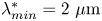 $\lambda _{{min}}^{*}= 2\ \mathrm {\mu }\textrm {m}$) than the coarsest mesh. Since only the noise perturbation – not the principal perturbation – seeds initial growth of
 $\mathcal {K}_{3}$, the finer-resolution simulations generally predict larger
 $u_3''$-fluctuation magnitudes than the coarsest-resolution simulation.
Anisotropy metrics, Taylor microscales and Taylor Reynolds numbers in the baseline simulations: (a) plots  $\mathcal {Y}_{1}$ from (4.7); (b) plots the ratio
 $\lfloor {\mathcal {K}_2} \rfloor /\lfloor {\mathcal {K}_3} \rfloor$ of the mixing-layer integrals of the spanwise MDTKE components from (4.6) and (3.22); (c) and (d) plot, at 30 and 45 ns, respectively, the mixing-layer centre-plane autocorrelation functions (4.8a,b) calculated directly from the finest-resolution simulation (Sim), along with parabolic fits (Fit); (e) plots the
 $y$- and
 $z$-direction Taylor microscales
 $\lambda _{t,i}$ from (4.10); and (f) plots the effective spanwise-direction Taylor Reynolds number
 $Re_{t,23}$ from (4.12). In (c,d), only values of
 $R_i$ at
 $r<2\ \mathrm {\mu }\textrm {m}$ were used to fit the analytic form (4.10). In all legends and headers, numbers state
 $\mathcal {N}_{yz,2}$ as defined in the caption of table 1, and the letters
 $y$ and
 $z$ correspond to the coordinate indices 2 and 3, respectively.

To further explore the structure of the mixing layer in the two spanwise directions, we consider length scales and dimensionless numbers based on the  $u_2$ and
 $u_3$ velocity components, at the mixing-layer centre-plane
 $x=x_c$ defined by (4.3). We draw on the analytical approaches of Weber et al. (Reference Weber, Haehn, Oakley, Rothamer and Bonazza2014b) in their experimental study of the RM instability and Cook & Dimotakis (Reference Cook and Dimotakis2001) in their computational study of the RT instability. Define the centre-plane
 $y$- and
 $z$-direction autocorrelation functions
 \begin{equation} R_{2}( r)= \frac{ \overline{ u_2( x_c, y, z) u_2( x_c, y + r, z)} }{ \overline{ u_2( x_c, y, z)^2}}, \quad R_{3}( r)= \frac{ \overline{ u_3( x_c, y, z) u_3( x_c, y , z+ r)} }{ \overline{ u_3( x_c, y, z)^2}}. \end{equation}
The corresponding  $y$- and
 $z$-direction Taylor microscales (Tennekes & Lumley Reference Tennekes and Lumley1972; Pope Reference Pope2000; Davidson Reference Davidson2015) can be defined from the curvature of
 $R_2$ and
 $R_3$, respectively
 \begin{equation} \lambda_{t,i} = \left( -\frac{1}{2} \left.\frac{ \textrm{d}^2 R_i}{\textrm{d} r^2} \right|_{r=0} \right)^{-1/2}. \end{equation}
In the present study, we calculate  $\lambda _{t,i}$ by fitting a parabola
 \begin{equation} R_{i,{fit}} = 1 - \frac{r^2}{ \lambda_{t,i}^2} \end{equation}
to  $R_i(r)$ over a small interval near
 $r=0$. Figures 13(c) and 13(d) show examples of
 $R_i$ and
 $R_{i,{fit}}$ calculated from the finest-resolution baseline simulation at a late pre-reshock time and a late post-reshock time. The Taylor microscales evoke definitions of centre-plane Taylor Reynolds numbers based on MDTKE-component velocities
 \begin{equation} Re_{t,i} = \frac{ \bar{\rho} \lambda_{t,(i)}}{ \overline{\mu}} \left( \frac{ 2 \mathcal{K}_{(i)}}{\bar{\rho}} \right)^{1/2}, \end{equation}
with no summation on  $i$ implied. An effective spanwise-direction Taylor Reynolds number can also be defined by
 \begin{equation} Re_{t,23}= \frac{Re_{t,2} + Re_{t,3}}{2}. \end{equation}
Compare (39a) and (39b) in Cook & Dimotakis (Reference Cook and Dimotakis2001).
Figures 13(e) and 13(f) plot time histories of the  $y$- and
 $z$-direction Taylor microscales and the effective spanwise-direction Taylor Reynolds number in the three baseline simulations. For each simulation, the
 $y$-direction microscale
 $\lambda _{t,2}$ is always larger than the corresponding
 $z$-direction microscale
 $\lambda _{t,3}$. Hence, as also observed in figure 13(b), there are persistent differences in the mixing-layer structure along the two spanwise directions, even at late times. The post-reshock Taylor Reynolds number
 $Re_{t,23}$ is significantly larger than 100–140, suggesting that the flows meet the criterion proposed by Dimotakis (Reference Dimotakis2000) for transition to a well-mixed turbulent state. (Zhou (Reference Zhou2007) argues that additional, more stringent conditions must also be met for non-stationary flows.) However, both the microscales and Reynolds number are moderately sensitive to the mesh (particularly after reshock) and have not reached their DNS limits in the present study. Any definitive conclusions based on absolute values of
 $\lambda _{t,2}$,
 $\lambda _{t,3}$ and
 $Re_{t,23}$ would require greater resolution and/or more advanced computational schemes, e.g. less-dissipative, higher-order numerics or explicit SGS models. We also reiterate that the turbulent energy spectra of figure 12(b) do not exhibit broad inertial ranges; such ranges may or may not appear with greater resolution and/or more advanced computational schemes.
4.6. Evolution of enstrophy
The vorticity  $\omega _i$ is the curl of the velocity
 $u_i$, i.e.
 $\omega _i = \epsilon _{ijk} \partial u_k/\partial x_j$, where
 $\epsilon _{ijk}$ is the antisymmetric Levi-Civita symbol (also called the permutation symbol or the alternating unit tensor). The enstrophy is a scalar measure of vorticity magnitude
 \begin{equation} \varOmega= \tfrac{1}{2} \omega_i \omega_i . \end{equation}
An evolution equation for  $\varOmega$ can be derived from the Navier–Stokes equations (3.3)
 \begin{align} \frac{ \partial}{\partial t} \left( \rho \varOmega \right) &+ \frac{ \partial}{\partial x_j} \left( \rho \varOmega u_j \right) =\underbrace{ \left( \rho \omega_j S_{ij} \omega_i \right) }_{ \mathbb{E}_{I}} + \underbrace{\left( -2\rho \varOmega \frac{ \partial u_j}{\partial x_j} \right)}_{ \mathbb{E}_{II}} \nonumber\\ &+ \underbrace{ \left( \frac{\omega_i}{\rho} \epsilon_{ijk} \frac{ \partial \rho}{\partial x_j} \frac{\partial p}{\partial x_k} \right) }_{ \mathbb{E}_{III}} + \underbrace{\left( \rho \omega_i \epsilon_{ijk} \frac{\partial}{\partial x_j} \left[ \frac{1}{\rho} \frac{\partial \sigma_{kl}}{\partial x_l} \right] \right)}_{ \mathbb{E}_{IV}} . \end{align}
Vorticity dynamics is important in instability growth, variable-density turbulent mixing and shock-wave–turbulence interaction (Andreopoulos, Agui & Briassulis Reference Andreopoulos, Agui and Briassulis2000; Chassaing et al. Reference Chassaing, Antonia, Anselmet, Joly and Sarkar2010). Analysis of vorticity and enstrophy in simulated non-HED mixing layers with reshock can be found in Schilling & Latini (Reference Schilling and Latini2010), Grinstein et al. (Reference Grinstein, Gowardhan and Wachtor2011), Hahn et al. (Reference Hahn, Drikakis, Youngs and Williams2011) and Tritschler et al. (Reference Tritschler, Olson, Lele, Hickel, Hu and Adams2014), which consider 3-D layers arising from multimode perturbations; Latini et al. (Reference Latini, Schilling and Don2007) and Schilling, Latini & Don (Reference Schilling, Latini and Don2007), which consider 2-D layers arising from single-mode perturbations; and Latini & Schilling (Reference Latini and Schilling2020), which considers both 2-D and 3-D layers arising from single-mode perturbations. Vorticity analysis also features prominently in the works on shock-wave–turbulence interaction by Larsson & Lele (Reference Larsson and Lele2009), Larsson, Bermejo-Moreno & Lele (Reference Larsson, Bermejo-Moreno and Lele2013), Ryu & Livescu (Reference Ryu and Livescu2014) and Livescu & Ryu (Reference Livescu and Ryu2016). The supplementary material provides a complete derivation of (4.14).
The terms on the right-hand side of (4.14) are labelled. The first term  $\mathbb {E}_{I}$ is the vortex-stretching term, accounting for stretching, shrinking and tilting of vortices. It vanishes for a 2-D flow. The second term
 $\mathbb {E}_{II}$ is the enstrophy–dilatation term, which vanishes for a constant-density flow (in which
 $\partial u_j/\partial x_j \equiv 0$). The third term
 $\mathbb {E}_{III}$ is the baroclinic source term, which generates enstrophy via misalignment of density and pressure gradients, e.g. in a flow with RM and RT instabilities. The fourth term
 $\mathbb {E}_{IV}$ is the dissipation term, which captures the dissipative action of viscosity via the viscous stress tensor
 $\sigma _{kl}$.
Figure 14(a) plots  $\lfloor {\rho \varOmega } \rfloor$, the mixing-layer integral of density-weighted enstrophy, versus time. Like
 $\lfloor {\mathcal {K}} \rfloor$ in figure 12(a),
 $\lfloor {\mathcal {\rho \varOmega }} \rfloor$ rises slowly after first shock, stabilizes, increases sharply by over one order of magnitude after reshock and finally decays as the mixing layer grows and decompresses. Table 4 quantifies the reshock-induced increase and the post-reshock decay at selected times. From 30 to 35 ns, the integrated density-weighted enstrophy increases by a factor of
 $\sim$30–70, much like the integrated MDTKE as reported in table 3. The sharp reshock-induced increase in enstrophy seen here is consistent with findings from the non-HED computational studies by Latini et al. (Reference Latini, Schilling and Don2007), Schilling et al. (Reference Schilling, Latini and Don2007) and Tritschler et al. (Reference Tritschler, Olson, Lele, Hickel, Hu and Adams2014). As also observed by those authors, enstrophy is much more sensitive to the mesh than turbulent kinetic energy. Indeed, at any given time,
 $\lfloor {\rho \,\varOmega } \rfloor$ increases with the density of computational zones. The ratio of post-reshock to pre-reshock
 $\lfloor {\rho \,\varOmega } \rfloor$ is less sensitive to the mesh than instantaneous values of
 $\lfloor {\rho \,\varOmega } \rfloor$.
In (a), evolution of the mixing-layer integral of density-weighted enstrophy  $\rho \varOmega$ from (4.13) in the three baseline simulations. The legend states
 $\mathcal {N}_{yz,2}$ as defined in the caption of table 1. In (b,c), evolution of the mixing-layer integrals of each term
 $\mathbb {E}_{I}, \ldots , \mathbb {E}_{IV}$ in (4.14), normalized by
 $\lfloor {\rho \varOmega } \rfloor$, in the finest-resolution baseline simulation: (b) displays early-time results before reshock, and (c) displays late-time results after reshock. Note the difference in the ordinate limits of the two figures. Equation (3.22) defines the mixing-layer integral.

Selected values of the mixing-layer integral of density-weighted enstrophy ( $\textrm {g}\,\textrm {cm}^{-3}\,\textrm {ns}^{-2}$) at three different times (ns). The ratio of the early post-reshock value to the late pre-reshock value and the ratio of the early post-reshock value to the late post-reshock value are given. Compare with figure 14(a).

To obtain deeper insight into growth and decay of the enstrophy, we examine mixing-layer integrals of each term on the right-hand side of (4.14). When normalized by  $\lfloor {\mathcal {\rho \,\varOmega }} \rfloor$, such integrals have units of inverse time and quantify the relative magnitude of the various mechanisms of enstrophy creation or destruction. Figure 14(b) plots the four quantities
 $\lfloor {\mathbb {E}_{I}} \rfloor /\lfloor {\rho \,\varOmega } \rfloor ,\ldots ,\lfloor {\mathbb {E}_{IV}} \rfloor /\lfloor {\rho \varOmega } \rfloor$ in the finest-resolution baseline simulation before reshock. The baroclinic source term dominates the enstrophy production just after first shock. This early-time production is offset by destruction due to the enstrophy–dilatation term, which is negative in areas of local fluid expansion (where
 $\partial u_j/\partial x_j > 0$). The contribution from the vortex-stretching term is initially small but grows steadily, eventually outweighing the contribution from the baroclinic source term. Enstrophy destruction due to the dissipation term occurs throughout pre-reshock growth, but its magnitude is small.
Figure 14(c) plots the same four quantities after reshock. As the reshock traverses the mixing layer, there is a sharp increase in enstrophy production due to both the baroclinic source and enstrophy–dilatation terms. The latter term is positive in areas of local fluid compression (where  $\partial u_j/\partial x_j < 0$). In fact,
 $\lfloor {\mathbb {E}_{II}} \rfloor$ exceeds
 $\lfloor {\mathbb {E}_{III}} \rfloor$ during the reshock traversal, suggesting that fluid compressibility has a significant role in vorticity generation during reshock. After the reshock exits the mixing layer, enstrophy production is principally due to the vortex-stretching term. At very late time, enstrophy–dilatation production increases again as the reflected main shock compresses the mixing layer. The sum of the four mixing-layer integrals
 $\lfloor {\mathbb {E}_{I}} \rfloor , \ldots , \lfloor {\mathbb {E}_{IV}} \rfloor$ is positive at all times after reshock, suggesting that the post-reshock decay of
 $\lfloor {\rho \varOmega } \rfloor$ is attributable to numerical dissipation and/or redistributive mechanisms involving the left-hand side of (4.14), e.g. entrainment of zero-enstrophy unmixed fluid into the developing mixing layer. The fact that the mixing layer undergoes intense post-reshock decompression, as discussed in § 4.3 and in contrast to typical non-HED analogues, also points to the importance of advective redistribution.
Figures 14(b) and 14(c) only plot results from the finest-resolution baseline simulation. The supplementary material provides corresponding results from the two lower-resolution baseline simulations. Qualitative trends in the normalized mixing-layer integrals  $\lfloor {\mathbb {E}_{I}} \rfloor /\lfloor {\rho \varOmega } \rfloor ,\ldots ,\lfloor {\mathbb {E}_{IV}} \rfloor /\lfloor {\rho \varOmega } \rfloor$ in the two lower-resolution cases are mostly the same as those observed in the finest-resolution case, with one important exception:
 $\lfloor {\mathbb {E}_{I}} \rfloor /\lfloor {\rho \varOmega } \rfloor$ is significantly smaller with coarser meshes, particularly at late pre-reshock and early post-reshock times. We suspect that the finest-resolution simulation better resolves the 3-D physics of vortex stretching, just as it better resolves the growth of initially small
 $z$-direction velocity fluctuations as discussed in § 4.5.
Moreover, it is important to emphasize that (4.14) is not exact for an under-resolved 3-D simulation. Numerical errors arise both from the discretization of the governing equations within Ares and from the use of finite differences during post-processing, e.g. to compute  $\varOmega$ from
 $u_i$. For a detailed examination of numerical errors,
 $\varOmega$ could be replaced in (4.14) with
 $\breve { \varOmega }+ \mathfrak {T}_{\varOmega }$, where
 $\varOmega$ is the exact solution to the system of partial differential equations (3.1)–(3.6) with (4.13),
 $\breve {\varOmega }$ is the numerical solution obtained from the post-processed simulation and
 $\mathfrak {T}_{\varOmega }$ is the truncation error. Similar substitutions could be made for all flow variables and their derivatives. Then, a new equation could be derived that would resemble (4.14), except for the addition of truncation error terms that vanish in the DNS limit. The procedure outlined here draws on the theory of equivalent or modified differential equations, foundational to computational fluid dynamics (Hirsch Reference Hirsch2007, § 7.1). Truncation errors associated with enstrophy evolution were recently analysed by Zhou, Groom & Thornber (Reference Zhou, Groom and Thornber2020) in simulations of shocked non-HED mixing layers. In the present study, the grid independence of several trends mentioned above – e.g. the larger production during reshock via the enstrophy–dilatation term than via the baroclinic source term – suggests that they are physically meaningful and not merely numerical artefacts. Nevertheless, further analysis of numerical errors is warranted, particularly of their role in the post-reshock enstrophy decay.
5. Results and analysis: CPVs
This section discusses the CPVs, a set of simulations that do not include electron thermal conduction. The CPVs are motivated by the observation in § 2 that the baseline HED flow exhibits much lower conductive Péclet numbers than a canonical non-HED analogue, due to energy transport by ionized electrons (present only in the HED case). Generally, thermal conduction is much more efficient via interactions involving free electrons than via heavy-particle collisions, i.e. ion–ion or neutral-atom–neutral-atom collisions. By comparing the CPVs and the baseline simulations, we aim to isolate and understand the influence of electron thermal conduction on HED shock-induced mixing. For other pertinent discussions of small-scale temperature fluctuations in mixing plasmas in an ICF context, see the recent work by Morgan et al. (Reference Morgan, Olson, Black and McFarland2018) and Haines et al. (Reference Haines2020).
Like the baseline simulations, the CPVs are executed using three different-resolution meshes. For a given resolution, the designs of the baseline simulation and the corresponding CPV are identical in every respect except for the inclusion or not of electron thermal conduction. AMR parameters (summarized in table 1), boundary conditions (illustrated in figure 3) and the interface initial perturbation (illustrated in figure 4) are the same. Main-shock and reshock trajectories are nearly identical, as shown in appendix B. The computational cost of the CPV is slightly less than that of the baseline simulation.
Some preliminary concepts are needed. First, define the Prandtl number at the mixing-layer centre-plane
 \begin{equation} Pr_c = \left.\frac{ \overline{\mu}\, \overline{c}_{p,{eff}}}{ \overline{\kappa}_{eff}} \right|_{x=x_c}, \end{equation}
where  $c_{p,{eff}}$ is the specific effective total heat capacity at constant pressure and
 $x_c$ is defined by (4.3). For a plasma with
 $T_n \approx T_e$ (see § 4.3),
 $c_{p,{eff}}$ is estimated as
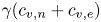 $\gamma ( c_{v,n} + c_{v,e} )$, where
 $c_{v,n}= ( \partial \mathcal {E}_n/\partial T_n )_{\rho }$ and
 $c_{v,e}= (\partial \mathcal {E}_e/\partial T_e )_{\rho }$ are the specific ion and electron heat capacities at constant volume, respectively, and
 $\gamma = 5/3$ is the heat capacity ratio for a monatomic gas (Schroeder Reference Schroeder2000; Anderson Reference Anderson2003). The effective total thermal conductivity is
 \begin{equation} \kappa_{eff}= \begin{cases} \kappa_n+ \kappa_e, & \text{for baseline simulations}, \\ \kappa_n, & \text{for CPVs}. \end{cases} \end{equation}
Other definitions are possible, since the concept of an effective total thermal conductivity is not immediately apparent from (3.1)–(3.6). We claim that (5.2) is reasonable, especially because  $\kappa _e \gg \kappa _n$ in the baseline-simulation mixing layers, i.e. the ion thermal conductivity contributes negligibly to the effective total. Next, define the effective spanwise-direction Taylor conductive Péclet number
 \begin{equation} {Pe}^{(c)}_{t,23}= Re_{t,23} Pr_c , \end{equation}
where  $Re_{t,23}$ is the Reynolds number at the centre-plane from (4.12). Note that
 ${Pe}^{(c)}_{t,23}$ does not explicitly depend on viscosity
 $\overline {\mu }$. It is the ratio of an advective rate of heat transfer – based on the Taylor microscale and the spanwise-direction MDTKE-component velocities – to the rate associated with thermal conduction. The emphasis here on
 ${Pe}^{(c)}_{t,23}$, not
 $Pr_c$, is deliberate and important. As discussed in § 4.4, our simulations do not resolve the scales of viscous dissipation. Conversely, as discussed in §§ 4.1 and 4.5, they give reasonable (though not perfectly grid-converged) estimates of larger scales like the mixing-layer width and the Taylor microscale. Hence, we claim that the simulations are better suited for comparisons of advective and conductive heat-transfer rates (associated with
 ${Pe}^{(c)}_{t,23}$) than for comparisons of momentum and thermal diffusivities (associated with
 $Pr_c$).
In a similar way, define the Schmidt number at the mixing-layer centre-plane
 \begin{equation} {{Sc}}_c = \left.\frac{ \overline{\mu}}{\bar{\rho}\,\overline{D}} \right|_{x=x_c}, \end{equation}
and define the effective spanwise-direction Taylor diffusive Péclet number
 \begin{equation} {Pe}^{(d)}_{t,23}= Re_{t,23} {{Sc}}_c , \end{equation}
which does not explicitly depend on  $\overline {\mu }$. Extending the arguments of the previous paragraph, we claim that our simulations are better suited for comparisons of advective and diffusive mass-transfer rates (associated with
 ${Pe}^{(d)}_{t,23}$) than for comparisons of momentum and mass diffusivities (associated with
 ${{Sc}}_c$).
Figure 15 compares various quantities in the three baseline simulations and the three CPVs. Figure 15(a) plots the conductive Péclet number  ${Pe}^{(c)}_{t,23}$ from (5.3), showing the expected trends: at a given resolution and at any time,
 ${Pe}^{(c)}_{t,23}$ is approximately two orders of magnitude lower in the baseline simulation than in the CPV. For each set of three computations, variation in
 ${Pe}^{(c)}_{t,23}$ with mesh resolution is mainly attributable to variation in
 $Re_{t,23}$ rather than
 $Pr_c$. The figure suggests immediately that, in the baseline simulations but not in the CPVs, the scales of thermal conduction are comparable to the scales of advection within the mixing layers.
Comparisons of various metrics in the baseline simulations (Base) and the CPVs: (a) the conductive Péclet number  ${Pe}^{(c)}_{t,23}$ from (5.3); (b) the diffusive Péclet number
 ${Pe}^{(d)}_{t,23}$ from (5.5); (c) the mixed mass
 $\mathcal {M}$ from (4.1); (d) the normalized mixed mass
 $\varPsi$ from (4.2); (e) the mixing-layer integral of MDTKE
 $\mathcal {K}$ from (4.5); and (f) the mixing-layer integral of density-weighted enstrophy
 $\rho \varOmega$ from (4.13). In the supplementary material, movie 3 accompanies (e), and movie 4 accompanies (f). Lines with symbols denote CPV results, and lines without symbols denote baseline-simulation results. Equation (3.22) defines the mixing-layer integral. The legends state
 $\mathcal {N}_{yz,2}$ as defined in the caption of table 1. Some of the baseline-simulation results also appear in figures 8(a), 8(b), 12(a) or 14(a).

Figure 15(b) plots the diffusive Péclet number  ${Pe}^{(d)}_{t,23}$ from (5.5). At a given resolution and at any time,
 ${Pe}^{(d)}_{t,23}$ is large, and its value in the baseline simulation is comparable to its value in the CPV. The figure suggests that the scales of mass diffusion are small in a dimensional sense and are likely not well-resolved on these meshes.
Figures 15(c), 15(d), 15(e) and 15(f) plot the mixed mass  $\mathcal {M}$, normalized mixed mass
 $\varPsi$, mixing-layer integral of MDTKE
 $\mathcal {K}$ and mixing-layer integral of density-weighted enstrophy
 $\rho \varOmega$, respectively, all as defined in § 4. At a given resolution, the mixed mass is slightly larger in the CPV than in the baseline simulation, both before and after reshock. (The mixing-layer width
 $\mathcal {W}$ also shows the same behaviour.) The normalized mixed mass, after initial post-first-shock growth, is also larger in each CPV than in the corresponding baseline case. The differences are largest in the several ns after reshock; observe that the baseline-simulation decrement to
 $\varPsi$ (relative to the CPV) at 35 ns increases steadily with resolution. At a given resolution, the mixing-layer integrals of MDTKE in the CPV and the baseline simulation are quite similar, although some differences are notable at the coarsest resolution and/or at very late times. Conversely, there are substantial differences in the mixing-layer integrals of density-weighted enstrophy between the CPVs and the baseline cases, except at late post-reshock times. Across the three mesh resolutions, the baseline-simulation decrement to
 $\lfloor {\rho \varOmega } \rfloor$ (relative to the CPV) is significant but variable, ranging from
 $13\text { to }31\,\%$ at 30 ns and from
 $18$ to
 $29\,\%$ at 35 ns. For additional quantitative comparison of
 $\mathcal {M}$,
 $\varPsi$,
 $\lfloor {\mathcal {K}} \rfloor$ and
 $\lfloor {\rho \,\varOmega } \rfloor$ in the finest-resolution cases, see the selected values in table 5. The supplementary material includes animations accompanying figures 15(e) and 15(f): movie 3 shows centre-plane local density-weighted turbulent kinetic energy (
 $=\rho \mathcal {I}$), and movie 4 shows centre-plane density-weighted enstrophy (
 $=\rho \varOmega$).
Selected values, at three different times, of various metrics in the finest-resolution baseline simulation (Base) and the finest-resolution CPV. The same metrics plotted in figures 15(c), 15(d), 15(e) and 15(f) are considered here.

Taken together, the observations in the previous paragraph indicate that depriving the flow of electron thermal conduction leads to a minor but unequivocal increase in sub-zonal mixing. The effect emerges at moderate times after first shock, grows after reshock and persists weakly to late times. Accompanying the increase in sub-zonal mixing is an increase in the magnitude of vorticity. With electron thermal conduction removed, the enhancement of mixing-layer vorticity begins almost immediately after first shock, continues through reshock and lessens at later times. The trends are seen at all mesh resolutions, and they appear even though the strengths of the main shock and reshock are essentially unaffected by electron thermal conduction; see appendix B.
To illuminate the connection between electron thermal conduction and mixing, first consider any non-negative flow variable  $\phi$ and define the spanwise gradient squared magnitude operator
 \begin{equation} \mathcal{G}_{yz}^2 \phi \equiv \left( \frac{ \partial \phi}{\partial y} \right)^2 + \left( \frac{ \partial \phi}{\partial z} \right)^2. \end{equation}
For the present study, the axial component of the gradient of  $\phi$ is excluded, since it can be dominated by the bulk-flow inhomogeneities discussed in § 4.3. Associated with
 $\mathcal {G}_{yz}^2$ are the spanwise gradient inverse squared scale length
 $(\mathcal {G}_{yz}^2 \phi )/\phi ^2$, which has units of inverse squared length and is abbreviated SGISL, and the spanwise gradient inverse scale length
 ${(\mathcal {G}_{yz}^2 \phi )}^{1/2}/\phi$, which has units of inverse length and is abbreviated SGIL. These quantities are large when the magnitudes of spanwise components of the gradient are large, i.e. when
 $\phi$ exhibits sharp spanwise-direction variations with small characteristic lengths.
Figure 16 compares the mixing-layer averages of the SGISLs of four flow variables in the finest-resolution baseline simulation and CPV. The averaged SGISLs of  $\mathbb {M}_H$ mass fraction and total pressure (figures 16(a) and 16(b), respectively) in the baseline simulation are similar to those in the CPV, especially after reshock. In contrast, beginning immediately after first shock and persisting to late times, the averaged SGISL of electron temperature (figure 16d) is significantly larger in the CPV than in the baseline case. This trend is not surprising: activating electron thermal conduction enhances heat transfer from relatively hot to relatively cold fluid, which tends to soften or ‘smooth out’ local temperature gradients. Recall from § 4.3 that packets of the light material
 $\mathbb {M}_L$ tend to be much hotter that nearby packets of the heavy material
 $\mathbb {M}_H$ in the mixing layer. Perhaps more surprising is the trend shown in figure 16(c): the averaged SGISL of density is also significantly larger in the CPV than in the baseline case. Indeed, inspection of the temperature and density fields shows a strong correlation between temperature and density gradient magnitudes. These findings suggest that, in this HED flow, enhanced heat transfer between different-temperature fluid packets promotes the expansion of the colder (typically higher-density) packet and/or the contraction of the hotter (typically lower-density) packet. Thus, activating electron thermal conduction tends to soften local gradients of both temperature and density. Note that the CPV–baseline-simulation differences in the density SGISLs are likely not due to differences in the behaviour of the diffusive mass flux vector
 $J_{a,j}$ from (3.8). If they were, then we would not expect to see, as in figure 16(a), such good agreement between the baseline-simulation and CPV SGISLs of
 $\mathbb {M}_H$ mass fraction.
Mixing-layer averages of the SGISLs of various flow variables in the finest-resolution baseline simulation (Base) and the finest-resolution CPV: (a)  $\mathbb {M}_H$ mass fraction
 $Y_H$, (b) total pressure
 $p$, (c) density
 $\rho$ and (d) electron temperature
 $T_e$. The SGISL is defined in terms of the
 $\mathcal {G}_{yz}^2$ operator; see (5.6) and the supporting discussion. Equation (3.21) defines the mixing-layer average. The legends state
 $\mathcal {N}_{yz,2}$ as defined in the caption of table 1.

Figure 17 further supports the claims made in the previous paragraph. Shown are the CPV–baseline-simulation ratios of the mixing-layer averages of the SGISLs of the same quantities considered in figure 16, at all three mesh resolutions. For a flow variable  $\phi$, this ratio is
 \begin{equation} \frac{\langle\!\langle {( \mathcal{G}_{yz}^2 \phi ) / \phi^2} \rangle\!\rangle_{CPV}}{ \langle\!\langle {( \mathcal{G}_{yz}^2 \phi ) / \phi^2} \rangle\!\rangle_{Base}}, \end{equation}
a metric of gradient-scale-length differences between two simulations with the same mesh parameters. Figure 17(a) shows that the CPV–baseline-simulation discrepancies in the  $\mathbb {M}_H$ mass-fraction spanwise gradients are small at all times and at all mesh resolutions. Figure 17(b) shows that these discrepancies for the total pressure spanwise gradients are somewhat larger before and during reshock, but diminish at late times. In contrast, figures 17(c) and 17(d) show that the averaged SGISLs of density and electron temperature are significantly larger in the CPVs than in the baseline simulations. For the medium- and fine-resolution cases, (i) both the density and electron temperature averaged-SGISL ratios are greater than 2 for much of the time both before and after reshock, and (ii) both ratios increase almost monotonically after reshock.
Ratios of the mixing-layer averages of the SGISLs of various flow variables for three different mesh resolutions. For each case, the ratio is of the instantaneous CPV value to the instantaneous baseline-simulation (Base) value. The ratio is always calculated from a pair of simulations with identical mesh parameters. The same four flow variables considered in figure 16 are considered here. See (5.6) and the supporting discussion. Equation (3.21) defines the mixing-layer average. The legends state  $\mathcal {N}_{yz,2}$ as defined in the caption of table 1.

Figure 18 provides an additional visualization of the trends described in figures 16(c) and 17(c). The SGIL of density is shown at a late pre-reshock time and two late post-reshock times, in the finest-resolution baseline simulation in figure 18(a) and the finest-resolution CPV in figure 18(b). The figures plot the local quantities at the mixing-layer centre-plane. Darker regions signify larger values of the density SGIL, i.e. sharper density gradients characterized by smaller scale lengths. At each of the three times, the CPV exhibits more locations with more intense gradients than the baseline simulation. The figure highlights that these density SGIL differences remain through the very end of the simulations, even after the mixing layer has been impacted by the reflected main shock after 45 ns. For a corresponding animation of density SGILs over time, see movie 5 in the supplementary material.
Visualizations of the SGIL of density  $\rho$ at the mixing-layer centre-plane
 $x=x_c$ in (a) the finest-resolution baseline simulation (Base) and (b) the finest-resolution CPV. In both simulations,
 $\mathcal {N}_{yz,2}=360$; see table 1. Contour plots are provided at 30, 45 and 50 ns. The SGIL is defined in terms of the
 $\mathcal {G}_{yz}^2$ operator; see (5.6) and the supporting discussion. Equation (4.3) defines the coordinate
 $x_c$. Movie 5 in the supplementary material accompanies this figure.

The mechanistic link between sharper density gradients, increased enstrophy production and greater sub-zonal mixing lies in the baroclinic source term  $\mathbb {E}_{III}$ in the enstrophy evolution equation (4.14). Indeed, at a given mesh resolution and when compared to the baseline simulation (after normalization by
 $\lfloor {\rho \varOmega } \rfloor$), the CPV exhibits greater enstrophy production via the baroclinic source term, beginning shortly after first shock and continuing at least until reshock. This magnification of the baroclinic source term is followed by magnification of the vortex-stretching term
 $\mathbb {E}_{I}$. At late times after reshock, baroclinic production contributes little to the overall enstrophy dynamics, and integrated density-weighted enstrophy in the CPV approaches the value in the baseline simulation. Nevertheless, CPV–baseline-simulation differences in the mixed mass and (especially) in the magnitudes of spanwise gradients of temperature and density persist long after reshock.
Thus, the analysis of this section underscores a set of interconnected physical processes in the HED flows of the Reshock Campaign. In principle, the connection between enhanced thermal conduction, smoother temperature and density gradients and diminished baroclinic enstrophy production exists in any compressible flow (in which the conservation of energy equation(s), EOSs and Navier–Stokes equations are tightly coupled). However, studies of non-HED shock-induced mixing typically and justifiably place little attention on the role of thermal conduction between fluid packets within mixing layers. The CPV–baseline-simulation comparisons of this section demonstrate that thermal conduction should not be ignored in HED shock-induced mixing, especially if any quantities of interest depend on the magnitudes of local temperature or density gradients. In the HED mixing layers considered here, the presence of ionized electrons induces thermal conductivities so large that local heat transfer has a non-negligible impact on small-scale mixing – an impact that can be observed in modern numerical simulations.
6. Conclusions
This paper discussed a computational investigation of shocked and reshocked multimaterial mixing layers in the HED regime, in which pressures exceeded 1 Mbar. The flows had a multimode initial perturbation at the interface between a heavy material  $\mathbb {M}_H$ (iodine-doped polystyrene plastic) and a light material
 $\mathbb {M}_L$ (carbonized resorcinol formaldehyde). After they were shocked, both materials were plasmas. Perturbations grew via the RM and RT instability mechanisms, and
 $\mathbb {M}_H$–
 $\mathbb {M}_L$ interpenetration and mixing occurred. The simulations were based on a series of experiments performed at the NIF that were part of the Reshock Campaign (Nagel et al. Reference Nagel2017). The experimental series was designed as an HED analogue of non-HED shock-tube studies of instability growth and turbulent mixing. The present study built on a long history of experimental and computational research on shock-induced mixing at both non-HED and HED conditions. While the HED regime poses tremendous modelling challenges, many insights can be gained using modern theories and numerical methods.
To model the NIF experiments, a 3-D computational framework was designed. Simulations were executed using the radiation hydrodynamics code Ares with AMR. They included treatments of distinct ion and free-electron internal energies, non-ideal EOSs, radiation transport and plasma-state models of the transport processes of mass diffusion, viscous dissipation and thermal conduction. Two critical aspects of the simulations were tuned to available data from the NIF experiments: radiation temperature boundary conditions were determined from measurements of the shock positions, and the interface initial perturbation was scaled based on measurements (Huntington et al. Reference Huntington, Raman, Nagel, MacLaren, Baumann, Bender, Prisbrey, Simmons, Wang and Zhou2020) of the mixing-layer width. The simulated perturbation was carefully designed such that it captured key features of the experimental perturbations and it converged to an analytic form under mesh refinement.
The simulated mixing layers were analysed in two parts. In the first part, we investigated the evolution of various statistical metrics – common in studies of turbulent mixing – from three different-resolution baseline simulations. The mixing-layer width increased after first shock, decreased during reshock compression, increased rapidly after reshock and decreased again at late time due to compression from a reflected shock. The mixed mass increased monotonically, and its post-reshock growth rate was generally much larger than its pre-reshock growth rate. The normalized mixed mass (a dimensionless measure of sub-zonal mixing to larger-scale entrainment) approached values of  $\sim$0.80–0.85 at late time. Integrated metrics of MDTKE and enstrophy both increased by over an order of magnitude after reshock. Axial-direction anisotropy in the MDTKE was strong before reshock, but weakened substantially after reshock. Many of these trends were consistent with computational studies of non-HED shock-induced mixing. In the HED flows, both the baroclinic source and enstrophy–dilatation terms made large contributions to enstrophy production during reshock, suggesting that fluid compressibility is important in the vorticity dynamics in the HED regime.
The simulations included models of physical viscosity and mass diffusivity. In principle, they would converge to the DNS limit under mesh refinement. However, the resolutions considered here were not sufficient to resolve all fluid-dynamical length scales. Therefore, we scrutinized the mesh sensitivity of all quantities of interest. The mixing-layer width, mixed mass, moderate-to-late-time normalized mixed mass and MDTKE were all only weakly sensitive to mesh resolution. The enstrophy – particularly its production via vortex stretching – was strongly dependent on the grid, although the relative magnitude of the reshock-induced enstrophy increase was less dependent. Analysis of anisotropy suggested that the poor convergence of some quantities might be attributable to inadequate resolution of the small-wavelength noise component of the initial perturbation. A time-varying Reynolds number based on Taylor microscales was moderately grid dependent. However, at post-reshock times, this Reynolds number – at all resolutions – was large enough to suggest that the flows realized at the NIF had met a criterion (Dimotakis Reference Dimotakis2000) for transition to a well-mixed state.
In the second part of the analysis, we sought to illuminate the role of HED-specific physics in shock-induced mixing. Compared to a canonical non-HED analogue (Vetter & Sturtevant Reference Vetter and Sturtevant1995; Hill et al. Reference Hill, Pantano and Pullin2006), the HED flow exhibited similar Reynolds numbers and diffusive Péclet numbers but much smaller conductive Péclet numbers due to efficient thermal conduction by free electrons. Motivated by this finding, we ran three additional simulations, termed CPVs, that were identical to the baseline simulations except that electron thermal conduction was removed. At a given resolution, the mixing-layer width, mixed mass and moderate-to-late-time normalized mixed mass were larger in the CPV than the baseline simulation by minor but unequivocal amounts. At pre-reshock and early post-reshock times, enstrophy was also larger in the CPV than the baseline simulation. We explained these trends by showing that local spanwise gradients of both temperature and density were (on average) significantly sharper in the CPV than in the baseline simulation, resulting in greater baroclinic production of enstrophy and sub-zonal mixing in the CPV than in the baseline simulation.
Thus, the CPV–baseline-simulation analysis yielded insights into HED flows like those realized in the NIF Reshock Campaign. When compared to their non-HED analogues, the HED flows are distinguished by several interrelated characteristics: (i) the presence of ionized electrons substantially raises the effective thermal conductivity in a dimensional sense; (ii) there is strong correlation between local temperature gradients and local density gradients in the mixing layers, with different-density fluid packets tending to have very different temperatures; (iii) electron thermal conduction plays a significant role in softening local gradients of both temperature and density; and (iv) this gradient-softening mechanism is associated with a minor but non-negligible decrement to baroclinic enstrophy production and small-scale mixing.
The research presented here will help inform future theoretical, experimental and computational inquiries. The present simulations leveraged state-of-the-art models from numerous areas of fluid mechanics, thermodynamics and plasma physics. While we believe that these models reasonably represented all relevant physical processes (especially after tuning to experimental data), further examination of model sensitivities is warranted. The simulations could be repeated with better resolution of the initial perturbation, higher-order numerical schemes, more-sophisticated EOSs or alternate approaches to thermodynamic equilibration in mixed zones. In HED flows more complex than those considered here, instability growth and mixing may be affected significantly by ion–electron non-equilibrium, non-diffusive radiation transport, magnetohydrodynamics and other physics. Many open questions remain, along with opportunities for fruitful experiments and 3-D simulations. We look forward to continued dialogue between the traditional fluid mechanics and HED science communities, in the ongoing quest to understand mixing at extreme conditions.
Supplementary material and movies
Supplementary material and movies are available at https://doi.org/10.1017/jfm.2020.1122.
Acknowledgements
The authors thank T.A. Brunner, A. Campos, A.W. Cook, M.A. Hohensee and G. Zimmerman for helpful discussions, and they thank S.A. MacLaren for critical leadership in the early development of the Reshock Campaign. The authors also thank many others that have contributed to the Reshock Campaign at large, especially the target fabrication and NIF operations teams; see Nagel et al. (Reference Nagel2017) and Huntington et al. (Reference Huntington, Raman, Nagel, MacLaren, Baumann, Bender, Prisbrey, Simmons, Wang and Zhou2020) for comprehensive acknowledgements. Figures and movies were created using Matplotlib (Hunter Reference Hunter2007) and VisIt (Childs Reference Childs2013). The authors sincerely thank the developers of these open-source tools. This document was prepared as an account of work sponsored by an agency of the United States government. Neither the United States government nor Lawrence Livermore National Security, LLC, nor any of their employees makes any warranty, expressed or implied, or assumes any legal liability or responsibility for the accuracy, completeness or usefulness of any information, apparatus, product or process disclosed, or represents that its use would not infringe privately owned rights. Reference herein to any specific commercial product, process or service by trade name, trademark, manufacturer or otherwise does not necessarily constitute or imply its endorsement, recommendation or favouring by the United States government or Lawrence Livermore National Security, LLC. The views and opinions of authors expressed herein do not necessarily state or reflect those of the United States government or Lawrence Livermore National Security, LLC, and shall not be used for advertising or product endorsement purposes. This work was performed under the auspices of the U. S. Department of Energy by Lawrence Livermore National Laboratory under Contract No. DE-AC52-07NA27344.
Declaration of interests
The authors report no conflict of interest.
Author contributions
The research described in this document was inherently multidisciplinary and required a team of significant size. All authors contributed significantly. J.D.B. provided the vision for the project (as a subset of the larger Reshock Campaign), organized the team of contributors, designed and executed all simulations, wrote all core routines for simulation pre- and post-processing, designed all tables, figures and movies and wrote all the text of the initial manuscript. All other authors reviewed and provided feedback on the manuscript. O.S., K.S.R., R.A.M. and B.J.O. served as the principal internal reviewers of the manuscript. O.S. provided strategic technical consulting at all phases of the effort. In particular, he advised on the analysis of turbulent kinetic energy, anisotropy and enstrophy. K.S.R. initially conceived of the Reshock Campaign (along with S.A. MacLaren), led the theoretical and computational design of many of the experiments and provided vision and leadership throughout the Reshock Campaign's history. In the present study, he particularly consulted on the interpretation and application of experimental data. R.A.M. consulted on the EOS, electron thermal conduction and multispecies mixture equilibration routines in Ares, many of which he implemented. He provided critical support to ensure robustness of these routines, including improvements to Ares specifically tailored to the present study. B.J.O. consulted on pre- and post-processing methods. In particular, he advised on algorithms for constructing the interface initial perturbation; the code written by J.D.B. to accomplish this task in the present study was based on earlier code by B.J.O. After J.D.B., O.S., K.S.R., R.A.M. and B.J.O., the authors are listed in alphabetical order. S.R.C. consulted on the mass diffusion and ion thermal conduction models and implemented the models in Ares. C.L.E. consulted on the viscosity and ion–electron energy coupling models and implemented the models in Ares, and he consulted on models of radiation diffusion. D.J.E. and C.E.W. analysed the Reshock Campaign's VISAR experiments and determined the main-shock and reshock breakout times. C.M.H. and S.R.N. led the experimental branch of the Reshock Campaign, including regular interactions with the target fabrication and NIF operations teams. For the present study, they determined all experimental mixing-layer widths from X-ray radiographs. B.E.M. consulted on pre- and post-processing methods, especially on techniques for extracting statistical quantities from simulations that include AMR. He also implemented and consulted on the proper use of periodic boundary conditions with AMR. S.T.P. provided leadership of both the experimental and computational branches of the Reshock Campaign. B.S.P. provided leadership of the overall Ares code project. He also provided critical support to ensure efficiency and robustness of the AMR routines for the present study. P.A.S. consulted on the EOS and electron thermal conduction models. He computed key EOS model parameters for all materials and benchmark values of the electron thermal conductivity. Y.Z. consulted on theoretical issues, particularly concerning turbulence length scales and mixing metrics.
Appendix A. Material properties: additional details
A.1. EOS of a single species
Expanding on § 3.2, this appendix further describes the EOSs of the three pure materials  $\mathbb {M}_H$,
 $\mathbb {M}_L$ and
 $\mathbb {M}_R$ as modelled in the present study. Each material is treated as a single species. In this appendix, all thermodynamic quantities and model coefficients are understood to be particular to a single species. Multispecies mixtures are discussed later in appendix A.4.
From (3.17) and (3.18), the total pressure  $p$ is expressed as the sum of the ion pressure
 $p_{n}$ and the electron pressure
 $p_{e}$, and the specific total internal energy
 $\mathcal {E}_l$ is expressed as the sum of the specific ion internal energy
 $\mathcal {E}_{n}$ and the specific electron internal energy
 $\mathcal {E}_{e}$. The concept of separating thermodynamic contributions due to ions and free electrons is discussed in detail by Zel'dovich & Raizer (Reference Zel'dovich and Raizer2002, §§ XI.1–XI.6) and Ramshaw & Cook (Reference Ramshaw and Cook2014). Importantly, whenever discussing material properties in this work, we adopt the following conventions. An electron internal energy like
 $\mathcal {E}_{e}$ always refers to an electron thermal internal energy, meaning that it is formally zero when the electron temperature
 $T_e = 0$. Conversely, an ion internal energy like
 $\mathcal {E}_{n}$ always refers to a sum of two sub-components: an ion thermal component (which is formally zero when the ion temperature
 $T_n = 0$) and a cold component (which is formally independent of temperature). Similar conventions are followed for
 $p_e$ and
 $p_n$.
In typical EOS formalisms for HED-flow calculations, the density  $\rho$, ion temperature
 $T_n$ and electron temperature
 $T_e$ are treated as independent variables. Then,
 $p_{n}$,
 $p_{e}$,
 $\mathcal {E}_{n}$, and
 $\mathcal {E}_{e}$ are defined as follows:
 \begin{align} p_{n} = p_{n} ( \rho, T_{n} ),\\ p_{e} = p_{e} ( \rho, T_e ),\\ \mathcal{E}_{n} = \mathcal{E}_{n} ( \rho, T_{n} ),\\ \mathcal{E}_{e} = \mathcal{E}_{e} ( \rho, T_{e} ). \end{align}
It is assumed (Ramshaw & Cook Reference Ramshaw and Cook2014) that  $p_n$ and
 $\mathcal {E}_n$ are independent of
 $T_e$ and that
 $p_e$ and
 $\mathcal {E}_e$ are independent of
 $T_n$.
For the present study, the QEOS model of More et al. (Reference More, Warren, Young and Zimmerman1988) is used to explicitly define the four functions in (A1a–d). QEOS was designed as a versatile description of matter at a wide range of densities and temperatures. For a material with fixed atomic number  $Z$ and atomic weight
 $A$, the total Helmholtz free energy per unit mass
 $F$ is expressed as the sum of three components
 \begin{equation} F( \rho, T_n, T_e )= F_1( \rho, T_n )+ F_2( \rho, T_e )+ F_3( \rho ), \end{equation}
where  $F_1$ is the ion component, a function of
 $\rho$ and
 $T_{n}$;
 $F_2$ is the electron component, a function of
 $\rho$ and
 $T_e$; and
 $F_3$ is the chemical bonding correction, a function of
 $\rho$ only. Pressures, specific internal energies and other thermodynamic quantities are calculated from
 $F$ using thermodynamic identities (McQuarrie Reference McQuarrie2000; Schroeder Reference Schroeder2000).
In the QEOS framework,  $F$ is constructed as a smooth function, and it exactly satisfies a condition of thermodynamic consistency (More et al. Reference More, Warren, Young and Zimmerman1988, (6)). The ion component
 $F_1$ is constructed analytically such that it reduces to well-known physical laws in various limiting cases, e.g. it reduces to the ideal gas law at high temperatures or low densities. The ion component is constrained by various material properties that are treated as model inputs, principally the Debye temperature (McQuarrie Reference McQuarrie2000, (11.27)), the Grüneisen gamma (Zel'dovich & Raizer Reference Zel'dovich and Raizer2002, § XI.4) and the melting temperature at a reference condition. The electron component
 $F_2$ is based on Thomas–Fermi theory (Feynman et al. Reference Feynman, Metropolis and Teller1949), which treats the material as nuclei surrounded by a charged semiclassical electron fluid including Fermi–Dirac electron statistics. At a given density and temperature,
 $F_2$ is determined by the atomic number
 $Z$ and the atomic weight
 $A$. The chemical bonding correction
 $F_3$ is constructed analytically. It adds an approximate treatment of chemical bonds that is absent in Thomas–Fermi theory and is particularly relevant at low temperatures and solid-state densities. The chemical bonding correction is expressed in terms of the bulk modulus, which can be calculated from the speed of sound (treated as a model input) at a reference condition. See Zel'dovich & Raizer (Reference Zel'dovich and Raizer2002, § XI.14) and Schroeder (Reference Schroeder2000, § 1.5).
In an efficient implementation of QEOS, some results from Thomas–Fermi theory are pre-computed and later recovered as needed via a table lookup. Hence, the model can overall be described as quasi-analytic. Also note that neither  $F_1$ nor
 $F_2$ reduce to zero in the limit of zero temperatures; they are not thermal components. Therefore, to obtain the specific electron (thermal) internal energy
 $\mathcal {E}_e$ in (A1d), we must take the specific internal energy derived from
 $F_2$ and subtract its value at
 $T_e = 0$. To obtain the specific ion (non-thermal) internal energy
 $\mathcal {E}_n$ in (A1c), we must take the specific internal energy derived from
 $F_1$ and add contributions derived from
 $F_2$ at
 $T_e = 0$ and from
 $F_3$. Similar manipulations are required for
 $p_e$,
 $p_n$ and other quantities.
Table 6 gives the chemical compositions and other QEOS model input parameters for the materials  $\mathbb {M}_H$,
 $\mathbb {M}_L$ and
 $\mathbb {M}_R$ in the present study. The parameters were obtained from existing tabular EOSs in the LEOS database, specifically L5442 for CHI, L5250 for CRF and L5460 for PAI. Those tabular EOSs were constructed using an approach similar to the QEOS framework but including some additional features (Young & Corey Reference Young and Corey1995). For each material, the speed of sound
 $c_{s,{ref}}$ was determined by interpolation on the tabular EOS. All other parameters were taken directly from the inputs used to originally construct the tabular EOS. The chemical compositions were modelling approximations informed by knowledge of how each real material was manufactured. For simplicity, only carbon was included in the chemical composition for
 $\mathbb {M}_L$, even though real CRF contains carbon plus small fractions of hydrogen and oxygen. We emphasize that access to the tabular EOS database is not needed to reproduce any of the results in this paper.
Material chemical compositions and other parameters, used in the QEOS model (More et al. Reference More, Warren, Young and Zimmerman1988):  $X(b)$ is the number fraction of chemical element
 $b$ and is assumed to be fixed at all positions and times for a given material;
 $Z$ is the atomic number and
 $A$ is the atomic weight, computed as number averages over the chemical elements and, in the table, rounded to the nearest 0.001 when appropriate;
 $\varGamma$ is the Grüneisen gamma;
 $\rho _{{ref}}$ is the reference density;
 $T_{{ref}}$ is the reference temperature;
 $p_{{ref}}$ is the reference pressure;
 $c_{s,{ref}}$ is the speed of sound at reference density and temperature;
 $T_m$ is the melting temperature at reference density; and
 $T_d$ is the Debye temperature. The reference conditions are used only for parameterizing the EOSs and are not the same as the initialization conditions in the simulations.

A.2. Degree of ionization of a single species
The degree of ionization  $Z^{*}$ of a single material is defined as the number of free electrons per nucleus. Here,
 $Z^{*}$ is specified by an analytic function, given in More (Reference More1991, table 1), of the density, electron temperature, atomic number and atomic weight. The same formula was also referenced and reprinted by Atzeni & Meyer-ter-Vehn (Reference Atzeni and Meyer-ter-Vehn2004, table 10.2). It is a fit to numerical results from Thomas–Fermi theory (Feynman et al. Reference Feynman, Metropolis and Teller1949). The electron number density
 $n_e$ is related to
 $Z^{*}$ by
 \begin{equation} n_e= \frac{ \rho Z^{*}}{ m}, \end{equation}
where  $m$ is the mass of a single atom, computable from the atomic weight. The quantities
 $Z^{*}$ and
 $n_e$ are important for calculating transport coefficients, as explained below.
A.3. Opacities of a single species
For use in (3.5), (3.6), and (3.16), the Rosseland and Planck mean opacities of a single material,  $\varkappa _r$ and
 $\varkappa _p$, respectively, are given by a simple analytic function of density and electron temperature suggested by Atzeni & Meyer-ter-Vehn (Reference Atzeni and Meyer-ter-Vehn2004, (10.127))
 \begin{equation} \varkappa_{\iota}= C_{1,\iota} \rho^{C_{2,\iota}} T_e^{C_{3,\iota}}, \quad \iota = r\text{ or }p. \end{equation}
Table 7 gives the coefficients  $C_{1,\iota }$,
 $C_{2,\iota }$ and
 $C_{3,\iota }$ used for each of the materials
 $\mathbb {M}_H$,
 $\mathbb {M}_L$ and
 $\mathbb {M}_R$. The coefficients were obtained by curve fitting to tabular opacity data, which, in turn, were based on the Opal code (Iglesias, Rogers & Wilson Reference Iglesias, Rogers and Wilson1992; Rogers & Iglesias Reference Rogers and Iglesias1992; Iglesias & Rogers Reference Iglesias and Rogers1996) and the super-transition-array theory (Bar-Shalom et al. Reference Bar-Shalom, Oreg, Goldstein, Shvarts and Zigler1989). The fitting parameters were adjusted until main-shock and reshock trajectories, when using (A4) in a simplified 1-D version of the 3-D simulations (see appendix B), were similar to those obtained when using the tabular opacities directly. The parameters in table 7 are not expected to give reasonable representations of the opacities in any physics environment that differs significantly from the one considered here. We emphasize that access to the tabular opacity data is not needed to reproduce any of the results in this paper.
Material opacity parameters used with (A4). Parameters labelled  $r$ correspond to Rosseland mean opacities. Parameters labelled
 $p$ correspond to Planck mean opacities. The units of the parameters
 $C_{1,\iota }$ are dependent on the corresponding values of the exponents
 $C_{2,\iota }$ and
 $C_{3,\iota }$.

A.4. Properties of multispecies mixtures
The present simulations allow for arbitrary mixtures of the three species  $\mathbb {M}_H$,
 $\mathbb {M}_L$ and
 $\mathbb {M}_R$ anywhere in the computational domain. Due to the complexity of the species EOSs, care is needed to ensure a robust approach to calculating thermodynamic properties in a mixed-material zone. Ramshaw (Reference Ramshaw2004) conducted theoretical studies of mixtures of partially ionized gases with non-ideal EOSs. Cook (Reference Cook2009) published a computational method for thermodynamic equilibration of mixtures characterized by one temperature. Ramshaw & Cook (Reference Ramshaw and Cook2014) then extended the method to two-temperature plasma mixtures, i.e. those featuring distinct ion and electron temperatures. The method of Ramshaw & Cook (Reference Ramshaw and Cook2014) is used in the present study and summarized here.
The mixture equilibration problem is formulated as follows. Consider a computational zone with a mixture of the  $N_s$ species. Suppose that
 $\rho$,
 $\mathcal {E}_n$,
 $\mathcal {E}_e$ and
 $\{Y_a\}$ are known, where
 $\rho$,
 $\mathcal {E}_n$ and
 $\mathcal {E}_e$ refer to densities and specific internal energies of the mixture in aggregate and where
 $Y_a$ is the ratio of the mass of species
 $a$ to the total mass in the zone. Define the volume fraction
 $\upsilon _a$ as the fractional volume occupied by species
 $a$ if it were artificially separated from all other species;
 $\upsilon _a$ is an auxiliary variable that evokes definition of the species-
 $a$ density
 \begin{equation} \rho_a = \frac{ \rho Y_a}{\upsilon_a}. \end{equation}
We now seek a solution to the following system of equations:
 \begin{gather} p_{m,a}( \rho_a, T_{n,a},\,T_{e,a} ) = p_{e,a}( \rho_a, T_{e,a} ) + \mathcal{B}( T_{e,a} ) \ p_{n,a}( \rho_a, T_{n,a} )= p_{m,{eq}} , \end{gather}
 \begin{gather}T_{n,a} ( \rho_a, \mathcal{E}_{n,a} ) = T_{n,{eq}}= T_{n} , \end{gather}
 \begin{gather}T_{e,a} ( \rho_a, \mathcal{E}_{e,a} ) = T_{e,{eq}}= T_{e} , \end{gather}
 \begin{gather}\sum_{a=1}^{N_s} \upsilon_a = 1, \end{gather}
 \begin{gather}\sum_{a=1}^{N_s} Y_a \mathcal{E}_{n,a} = \mathcal{E}_n , \end{gather}
 \begin{gather}\sum_{a=1}^{N_s} Y_a \mathcal{E}_{e,a} = \mathcal{E}_e . \end{gather}
Equations (A6), (A7) and (A8) codify the core proposition of Ramshaw & Cook (Reference Ramshaw and Cook2014): thermodynamic equilibrium is achieved when the mixture-controlling pressure  $p_{m,a}$, the ion temperature
 $T_{n,a}$ and the electron temperature
 $T_{e,a}$ of each artificially separated species-
 $a$ volume is the same. The subscript
 $\textit {eq}$ denotes the equilibrium condition. The mixture-controlling pressure is defined by (A6), where the blending function
 $\mathcal {B}(T_{e,a})$ is
 \begin{equation} \mathcal{B}( T_{e,a}) = \exp \left[ -\ln 2 \left( \frac{ T_{e,a}}{ T_g} \right)^2 \right], \end{equation}
where  $\ln 2$ is the natural logarithm of 2 and
 $T_g$ is a parameter called the blending transition temperature, here set to 5 eV. Observe that
 $\mathcal {B}( T_{e,a}= T_g)= 0.5$ and that
 $\mathcal {B}$ varies smoothly from 1 as
 $T_{e,a} \to 0$ to 0 as
 $T_{e,a} \to \infty$. Hence,
 $p_{m,a}$ equals the total pressure in the low-temperature limit but the electron pressure in the high-temperature limit. Indeed, Ramshaw (Reference Ramshaw2004) and Ramshaw & Cook (Reference Ramshaw and Cook2014) argue that accurate equilibration of hot plasma mixtures (with
 $T_{e,a} \gg 0$) should be based on free-electron thermodynamic properties, not the total pressure. Equation (A9) follows from the definition of
 $\upsilon _a$, and (A10) and (A11) define the mixture specific internal energies as weighted sums of the species-
 $a$ specific internal energies
 $\{\mathcal{E}_{n,a}\}$ and
 $\{\mathcal{E}_{e,a}\}$.
Equations (A6)–(A11) are  $3N_s + 3$ equations for
 $3N_s + 3$ unknowns:
 $\{\upsilon _a\}$,
 $\{\mathcal {E}_{n,a}\}$,
 $\{\mathcal {E}_{e,a}\}$,
 $p_{m,{eq}}$,
 $T_{n,{eq}}$ and
 $T_{e,{eq}}$. The system of equations involves both explicit and implicit evaluations of the single-species EOSs, which are written as functions of densities and temperatures per (A1a–d). For example,
 $p_{e,a}(\rho _a,T_{e,a})$ in (A6) is an explicit evaluation, while
 $T_{e,a}( \rho _a,\mathcal {E}_{e,a})$ in (A8) is an implicit evaluation. The equations are solved iteratively using the procedure described in Ramshaw & Cook (Reference Ramshaw and Cook2014), which incorporates a Newton–Raphson root-finding scheme (Press et al. Reference Press, Teukolsky, Vetterling and Flannery1992).
With the solution obtained, the total pressure of the mixture is (Ramshaw & Cook Reference Ramshaw and Cook2014, (38))
 \begin{equation} p = \sum_{a=1}^{N_s} \upsilon_a p_a, \quad p_a = p_{n,a} + p_{e,a}. \end{equation}
Note that  $p$ and
 $p_{m,{eq}}$ are identical only in the zero-electron-temperature limit. The specific ion enthalpy of species
 $a$, used in (3.4), is
 \begin{equation} h_{n,a}= \mathcal{E}_{n,a}+ \frac{p_{n,a}}{ \rho_a}. \end{equation}
For a multispecies mixture, the degree of ionization  $Z^{*}$ is computed as a number-fraction-weighted average of the species-
 $a$ degrees of ionization
 \begin{equation} Z^{*}= \sum_{a= 1}^{N_s} X_a Z_a^{*}. \end{equation}
The number fraction  $X_a$ of species
 $a$ is related to the mass fraction
 $Y_a$ by
 \begin{equation} X_a= \left.\frac{Y_a}{ m_a} \right/ \sum_{b=1}^{N_s} \frac{ Y_b}{ m_b}, \end{equation}
where  $m_a$ is the mass of a single atom of species
 $a$. The mixture electron number density is calculated from
 \begin{equation} n_e= \rho \sum_{a= 1}^{N_s} \frac{ Y_a Z_a^{*}}{ m_a}. \end{equation}
The mixture opacity is computed as a volume-fraction-weighted average of the species- $a$ opacities
 \begin{equation} \varkappa_{\iota}= \sum_{a= 1}^{N_s} \upsilon_a \varkappa_{\iota,a}, \quad \iota = r\text{ or } p. \end{equation}
A.5. Ionic transport coefficients
This appendix elaborates on the models used for physical transport processes involving ions, namely mass diffusion, viscous dissipation and ion thermal conduction. The associated transport coefficients are the mass diffusivity  $D$, viscosity
 $\mu$ and ion thermal conductivity
 $\kappa _n$, respectively. The theory of transport processes in fluids is extensive, and we only give a brief overview of the relevant concepts. See Chapman & Cowling (Reference Chapman and Cowling1970) and Hirschfelder et al. (Reference Hirschfelder, Curtiss and Bird1954) for thorough expositions.
The models for the three ionic transport processes are based on kinetic theory. Specifically, Chapman–Enskog theory (Chapman & Cowling Reference Chapman and Cowling1970) supplies approximate solutions to the Boltzmann equation for particle distribution functions, along with analytic expressions for the transport coefficients. These expressions are written in terms of collision integrals, which quantify the effects of pairwise interactions between particles. In the present study, ion–ion binary collisions are modelled using a screened Coulomb potential, representing ion repulsion moderated by a background of free electrons, as presented and analysed by Stanton & Murillo (Reference Stanton and Murillo2016). Their exposition includes analytic fits for the key collision integrals and related quantities needed to treat ionic transport in many HED environments.
The mass diffusivity  $D$ in (3.8) is modelled by (55) in Stanton & Murillo (Reference Stanton and Murillo2016). For model inputs such as the ion number density and ion reduced mass, local averages over all species are used. Thus,
 $D$ is treated as a mixture-averaged self-diffusion coefficient; binary diffusion coefficients
 $D_{a b}$ for each
 $a$–
 $b$ species pair are never calculated. Ellison et al. (Reference Ellison2018) have studied this approach, which they call the one-component plasma (OCP) approximation. It is a considerable simplification of the physics of multispecies diffusion, and it is expected to be most accurate for mixtures of ions with similar masses and charges. Ellison et al. (Reference Ellison2018) found that it gave reasonable order-of-magnitude results for an ICF-relevant flow. Specifically, they reported that diffusive mixing between various combinations of five atomic species was larger, in a majority of cases, when using the OCP approximation instead of higher-fidelity approaches. For additional discussion of self-diffusion, see Chapman & Cowling (Reference Chapman and Cowling1970, § 14.5) and Hirschfelder et al. (Reference Hirschfelder, Curtiss and Bird1954, § 8.2.d.ii).
The formulation (3.8) for the diffusive mass flux vector ignores pressure and thermal contributions to mass diffusion – sometimes called barodiffusion and thermodiffusion, respectively – as defined by Chapman & Cowling (Reference Chapman and Cowling1970, §§ 14.1 and 14.6) and Hirschfelder et al. (Reference Hirschfelder, Curtiss and Bird1954, § 8.1a). Generally, barodiffusion is significant when pressure gradient magnitudes are large and when the atomic weights of the diffusing species are very discrepant, and thermodiffusion is significant when temperature gradient magnitudes are large. However, in the cases considered by Ellison et al. (Reference Ellison2018), the impact of neglecting these two contributions appeared to be comparable to or less than the impact of grouping species into one or more subsets (as done in the OCP approximation). Also, their cases involved a converging geometry and pressures and temperatures orders of magnitude larger than those in the present study. Hence, the impact of neglecting barodiffusion and thermodiffusion is expected to be less in the present study than in Ellison et al. (Reference Ellison2018). We stress that the assessment of simplified models of mass diffusion in HED flows remains an active area of research.
The viscosity  $\mu$ in (3.9) of a single material is modelled by (60) in Bergeson et al. (Reference Bergeson, Baalrud, Ellison, Grant, Graziani, Killian, Murillo, Roberts and Stanton2019). Their theory builds on earlier work by Haxhimali et al. (Reference Haxhimali, Rudd, Cabot and Graziani2015) and considers the viscosity to be a quadrature sum of two components: a weak-coupling component derived from Stanton & Murillo (Reference Stanton and Murillo2016, (74)) and a strong-coupling component proposed by Murillo (Reference Murillo2008, (5)). The new model is designed to capture viscosity physics across a wide range of values of the plasma coupling parameter, a dimensionless ratio of Coulomb-interaction energy to thermal energy (Bergeson et al. Reference Bergeson, Baalrud, Ellison, Grant, Graziani, Killian, Murillo, Roberts and Stanton2019, (2)). The shocked and reshocked mixing layers in the present study are in the weakly-to-moderately coupled regime; they exhibit values of the plasma coupling parameter from
 $\sim$0.9 to 2. For a multispecies mixture,
 $\mu$ is calculated explicitly in terms of species-
 $a$ viscosities
 $\{\mu_a\}$ using an approximation due originally to Burgers (Reference Burgers1969, (21.4a)) and investigated by Haxhimali et al. (Reference Haxhimali, Rudd, Cabot and Graziani2015, (B10)) and Bergeson et al. (Reference Bergeson, Baalrud, Ellison, Grant, Graziani, Killian, Murillo, Roberts and Stanton2019, (64)).
The ion thermal conductivity  $\kappa _n$ in (3.12) of a single material is modelled by (81) in Stanton & Murillo (Reference Stanton and Murillo2016). For a multispecies mixture,
 $\kappa _n$ is calculated explicitly in terms of species-
 $a$ conductivities
 $\{\kappa_{n,a}\}$, using a formula analogous to (B10) in Stanton & Murillo (Reference Stanton and Murillo2016).
A.6. Electron thermal conductivities
Models of electron thermal conduction are based on a theoretical framework somewhat different from the one used to model ionic transport. In this appendix, we first give a brief conceptual overview of the model used for the electron thermal conductivity  $\kappa _e$ in (3.13). We discuss the applicability of the model. Then, we summarize its key equations and compare its predictions to benchmark data.
Influential work on electron transport in HED plasmas was conducted by Lee & More (Reference Lee and More1984). They obtained an expression for  $\kappa _e$ in a plasma of arbitrary composition, starting from the Boltzmann equation for the electron distribution function and – in an important innovation over earlier research – accounting for electron degeneracy. They presented the formula for
 $\kappa _e$ as a function principally of the electron temperature, density, and chemical potential, and they gave analytic forms (fit to numerical results) for the relevant quantities. They warned that their model overestimated
 $\kappa _e$ for low-
 $Z^{*}$ plasmas, because it did not account for electron–electron scattering. In the present study,
 $\kappa _e$ for a single material is calculated as the product of two factors: a conductivity
 $\kappa _{e,o}$ as presented by Lee & More (Reference Lee and More1984) and a correction factor
 $\mathcal {S}_e$ that accounts for electron–electron scattering. The analytic expression for
 $\mathcal {S}_e$ was previously presented by Managan (Reference Managan2015) and satisfies important theoretical limits. For a multispecies mixture,
 $\kappa _e$ is calculated using local averages of the model inputs, rather than as an explicit function of species-
 $a$ conductivities
 $\{\kappa_{e,a}\}$.
It is important to mention that the model for  $\kappa _e$ with (3.13) is not accurate when the electron temperature gradient scale length is much smaller than the mean free path for electron–ion collisions
 $\lambda _{en}$. In such cases, low-collisionality kinetic effects become significant and cause inhibition or ‘saturation’ of the electron heat flux. Such physics, notably important in the laser ablation of hohlraum walls in HED experiments, are commonly modelled by applying a limiter to the heat flux for electron thermal conduction. Cowie & McKee (Reference Cowie and McKee1977), Bell (Reference Bell1985) and Atzeni & Meyer-ter-Vehn (Reference Atzeni and Meyer-ter-Vehn2004, § 7.2) discuss these issues in detail. Using the methodology of Bell (Reference Bell1985), we find that the ratio of the averaged local gradient scale length of electron temperature to
 $\lambda _{en}$ in the shocked and reshocked mixing layers of the present study ranges from
 ${\sim }9\times 10^{3}$ to
 $2\times 10^{5}$, large enough to suggest that a limiter is not needed for a reasonable description of the electron heat flux. Note that the limiters discussed notionally in this paragraph are distinct from and should not be confused with the radiation diffusion flux limiter of (3.16).
To describe the single-species electron thermal conductivity model in more detail, first define the auxiliary variables
 \begin{equation} \varTheta = 1 + \exp\left( -\frac{\varphi}{ k_b T_e }\right), \quad \vartheta = \ln\left[ 1 + \exp\left( \frac{\varphi}{ k_b T_e }\right)\right], \quad \chi = \frac{1}{Z^{*} \left( 1 + \vartheta \right)} , \end{equation}
where  $k_b$ is the Boltzmann constant (
 $\approx 1.381\times 10^{-16}\ \textrm {erg}\,\textrm {K}^{-1}$),
 $T_e$ is the electron temperature,
 $Z^{*}$ is the degree of ionization (i.e. the number of free electrons per nucleus) and
 $\varphi$ is the electron chemical potential. The electron thermal conductivity is
 \begin{equation} \kappa_e = \kappa_{e,o} \mathcal{S}_e. \end{equation}
The first factor is taken exactly from Lee & More (Reference Lee and More1984, (23b) and (24)), written in the Gaussian (rather than SI) system of units
 \begin{equation} \kappa_{e,o} = \frac{ 3 k_b \left( k_b T_e \right)^{5/2} \mathcal{A}} {2^{3/2} {\rm \pi}{ Z^{*}} e^4 m_e^{1/2} \ln \varLambda} \varTheta \mathcal{F}_{1/2}, \end{equation}
where  $e$ is the charge of an electron (
 $\approx 4.803\times 10^{-10}$ statcoulombs),
 $m_e$ is the mass of an electron and
 $\ln \varLambda$ is the dimensionless Coulomb logarithm for electron–ion collisions. The Coulomb logarithm is set according to Lee & More (Reference Lee and More1984, (17)). Other choices are possible; see Atzeni & Meyer-ter-Vehn (Reference Atzeni and Meyer-ter-Vehn2004, § 10.9.1) for further discussion. The factor
 $\mathcal {A}$ is expressed as a function of
 $\vartheta$. Rather than using the fit specified by Lee & More (Reference Lee and More1984, table VII, column 3), we use a similar but newer fit proposed by Managan (Reference Managan2015, (11))
 \begin{equation} \mathcal{A}( \vartheta) = \frac{ [128/(3 {\rm \pi})] + 2.4905 \vartheta + 0.53536 \vartheta^2 + 0.089107 \vartheta^3}{ 1 + 0.63389 \vartheta + 0.15998 \vartheta^2 + 0.089107 (3/{\rm \pi}^2) \vartheta^3}. \end{equation}
The quantity  $\mathcal {F}_{1/2}$ is a Fermi–Dirac integral (Lee & More Reference Lee and More1984, (26))
 \begin{equation} \mathcal{F}_{1/2} = \mathcal{F}_{1/2} \left( \frac{ \varphi}{k_b T_e} \right) = \int_{0}^{\infty} \frac{ s^{1/2}\,\textrm{d}s}{ 1 + \exp \left[ s - \varphi / ( k_b T_e ) \right]}. \end{equation}
Rather than evaluating  $\mathcal {F}_{1/2}$ directly via numerical integration, we use a curve fit (Managan Reference Managan2015, (20)) for the product
 $\varTheta \mathcal {F}_{1/2}$
 \begin{equation} \varTheta \mathcal{F}_{1/2} = \frac{\sqrt{\rm \pi}}{2} + \frac{ \vartheta^{1/2} \left[ 0.080897 + 0.99341 \vartheta - 0.20639 \vartheta^2 + 1.0710 (2/3) \vartheta^3 \right] }{ 1 + 0.11000 \vartheta + 1.0710 \vartheta^2}. \end{equation}
The electron–electron scattering correction factor  $\mathcal {S}_e$ is expressed as a function of
 $\chi$ (Managan Reference Managan2015, (37))
 \begin{equation} \mathcal{S}_e( \chi)= \left( \frac{ 0.0961}{1.2000} \right) \left( \frac{ 1.2000 + 5.4053 \chi + 4.4080 \chi^2 + 0.9067 \chi^3 }{ 0.0961 + 0.7778 \chi + 1.5956 \chi^2 + 1.3008 \chi^3} \right). \end{equation}
This relation is similar to an expression, derived from a general moment equations analysis, that was published by Ji & Held (Reference Ji and Held2013,  $\hat {\kappa }^{e}_{\parallel }$ in table III). The formulae from both Managan (Reference Managan2015) and Ji & Held (Reference Ji and Held2013) were designed to reproduce benchmark values for low-
 $Z^{*}$ plasmas from Braginskii (Reference Braginskii1965, table 2), and they satisfy
 $\mathcal {S}_e \to 1$ as
 $Z^{*} \to \infty$.
It remains to specify the chemical potential or, equivalently, the auxiliary variable  $\vartheta$. See Schroeder (Reference Schroeder2000, § 7.3) for an overview of the theory of the chemical potential of a degenerate Fermi electron gas. Here we use a fit that satisfies theoretical limits in the high-temperature (non-degenerate) and low-temperature (degenerate) extremes. Define the dimensionless Fermi energy
 \begin{equation} \varepsilon_f = \frac{ \hbar^2 ( 3 {\rm \pi}^2 n_e )^{2/3}}{ 2 m_e k_b T_e}, \end{equation}
where  $\hbar$ is Planck's constant (
 $\approx 6.626\times 10^{-27}\ \textrm {erg}\,\textrm {s}$) divided by
 $2 {\rm \pi}$ and
 $n_e$ is the electron number density. Let
 $\varsigma _f= \sqrt {\varepsilon _f}$. Then a reasonable approximation for
 $\vartheta$ as a function of
 $\varsigma _f$ is (Managan Reference Managan2015, (15))
 \begin{equation} \vartheta( \varsigma_f ) = \frac{ \varsigma_f^3 \left( [4/(3 \sqrt{\rm \pi})] + 0.19972 \varsigma_f + 0.17258 \varsigma_f^2 + 0.14500 \varsigma_f^3 \right)}{ 1+ 0.25829 \varsigma_f + 0.28756 \varsigma_f^2 + 0.16842 \varsigma_f^3 + 0.14500 \varsigma_f^4}. \end{equation}
For illustration and critical comparison, figure 19 plots selected thermal conductivity values for carbon at temperatures from 3 to 60 eV and densities from 0.2 to  $4.0\ \textrm {g}\,\textrm {cm}^{-3}$. Those ranges fully encompass the conditions in the simulated shocked and reshocked mixing layers; see figure 11. The material properties of carbon are important in the simulated flows, since carbon composes
 $100\,\%$ of
 $\mathbb{M}_L$ and
 $50\,\%$ of
 $\mathbb {M}_H$ per table 6. Figure 19(a) shows electron thermal conductivities calculated using the Ares model described above and the Purgatorio EOS code. Purgatorio uses a framework that (unlike the Ares model) accounts for the effects of electron shell structure (Hansen et al. Reference Hansen, Isaacs, Sterne, Wilson, Sonnad and Young2006; Wilson et al. Reference Wilson, Sonnad, Sterne and Isaacs2006; Sterne et al. Reference Sterne, Hansen, Wilson and Isaacs2007). The Purgatorio results are expected to be of higher fidelity than those from the Ares model, and the former are treated here as benchmark data. The figure shows that the Ares model successfully captures overall trends in
 $\kappa _e$, which varies by more than two orders of magnitude. However, near the upper bound of the temperature range, the Ares model can overestimate
 $\kappa _e$ by as much as
 $\sim$70 %. (Ares–Purgatorio discrepancies are even larger at temperatures below 3 eV.) Figure 19(b) compares Ares electron thermal conductivities with Ares ion thermal conductivities. The latter are calculated using the model described in appendix A.5. As expected, across the temperature and density ranges, the electron thermal conductivity vastly exceeds the ion thermal conductivity.
Comparisons of thermal conductivities versus temperature  $T$ at constant density
 $\rho$ for elemental carbon: (a) plots the electron thermal conductivities
 $\kappa _e$ from Ares and Purgatorio using lines and symbols, respectively, and (b) plots the electron thermal conductivity
 $\kappa _e$ from Ares (
 $e$) and the ion thermal conductivity
 $\kappa _n$ from Ares (
 $n$). Ion and electron temperatures are assumed to be equal, i.e.
 $T= T_e = T_n$. The Ares data are calculated with the models described in appendices A.5 and A.6, exactly as implemented in the 3-D fluid simulations. In the legends, numbers indicate the density in
 $\textrm {g}\,\textrm {cm}^{-3}$.

Appendix B. Consistency of simulated shock trajectories
For any comparative computational study of shock-induced mixing, it is natural to ask whether differences between simulations are due simply to differences in the shock strengths. This appendix provides evidence that, in fact, the main-shock and reshock trajectories are very similar across all the simulations considered in this work.
To analyse the position and velocity histories of the shocks, it proved useful to construct simplified 1-D versions of the 3-D simulations. Each 1-D simulation featured a  $\mathcal {N}_{x,2} \times 1 \times 1$ mesh, where
 $\mathcal {N}_{x,2}$ is the number of zones counted linearly along the
 $x$ direction on the finest AMR level in the corresponding 3-D simulation; see table 1. The 1-D simulations used a uniform mesh without AMR, with the same total
 $x$-extent
 $W$ as their 3-D counterparts. Sources
 $T_{r,{main}}$ and
 $T_{r,{reshock}}$ were applied in the 1-D simulations in exactly the same manner as in the 3-D simulations. The 1-D simulations were particularly conducive to shock-tracking methods based on characteristics (Anderson Reference Anderson2003), and they had an important role in the source-tuning procedure discussed in § 3.6.1.
Figure 20 compares main-shock and reshock trajectories from several cases, with time histories of position plotted in figure 20(a) and time histories of velocity plotted in figure 20(b). Included are results from coarse-, medium- and fine-resolution 1-D versions of both the baseline simulations and the CPVs. The shock velocity in these 1-D simulations is calculated directly from the characteristics-based method, not from a numerical derivative of shock position. Also included in figure 20(a) are selected shock positions, determined by inspection of the instantaneous pressure fields, in the finest-resolution 3-D baseline simulation. The figure suggests that the shock trajectories in the present study are not sensitive to any of the following: (i) mesh resolution; (ii) inclusion of an electron thermal conduction model or not; or (iii) use of a 3-D mesh with AMR instead of a corresponding 1-D mesh without AMR. The small radiative precursor ahead of the reshock, discussed in § 4.3, is not discernibly altered by electron thermal conduction.
Shock trajectories from various simulations: (a) plots time  $t$ versus axial shock position
 $x_h$, and (b) plots the axial component
 $u_h$ of shock velocity versus time
 $t$. Open squares and hexagons denote main-shock and reshock positions, respectively, in the finest-resolution 3-D baseline simulation per table 1. Thick lines and thin lines denote main-shock and reshock quantities, respectively, in coarse-, medium- and fine-resolution simplified 1-D simulations, as explained in the text. The legend entries for the 1-D simulations state
 $\mathcal {N}_{x,2}$, the number of zones counted linearly along the
 $x$ direction; compare with values in table 1. Base indicates a 3-D or 1-D simulation including electron thermal conduction, and CPV indicates a 1-D simulation excluding electron thermal conduction.

Appendix C. Coefficients for sources
Table 8 gives the coefficients used in (3.23) for the radiation temperature boundary conditions  $T_{r,{main}}$ and
 $T_{r,{reshock}}$. The constants were determined via the tuning procedure of § 3.6.1. The choices in table 8 are not unique; other choices could also yield suitable agreement with the NIF experimental data. Also, we caution the reader against over-attributing physical meaning to the tuned coefficients. They ensure that shock trajectories from the computational model are consistent with the experimental data, but they are not expected to give a general-purpose model of halfraum physics.
Coefficients used in (3.23) for the sources  $T_{r,{main}}$ and
 $T_{r,{reshock}}$.

Appendix D. Interface initial perturbation: additional details
This appendix explains how the principal-perturbation function  $\delta _x^{{\dagger} }$ and the noise-perturbation function
 $\delta _x^{{\dagger} }$ are defined for use in (3.24). Importantly,
 $\delta _x^{{\dagger} }$ and
 $\delta _x^{*}$ are designed such that their amplitudes are linearly proportional to constant dimensionless scaling parameters
 $\xi ^{{\dagger} }$ and
 $\xi ^{*}$, respectively. Those parameters can be related simply to the standard deviations
 $S^{{\dagger} }$ and
 $S^{*}$ of suitably large numbers of samples of the two functions. In the present study,
 $S^{{\dagger} }$ and
 $S^{*}$ were adjusted to achieve reasonable agreement with experimental measurements of the mixing-layer width; see § 3.6.2.
To construct the principal-perturbation function, let  $N^{{\dagger} }$ be an even number. Define a sequence of random lengths
 $(R_i)$, where each
 $R_i$ is independently sampled from a uniform distribution with
 $0\ \mathrm {\mu }\text {m}\leq R_i \leq 1\ \mathrm {\mu }\text {m}$, and define a corresponding sequence of positions
 $(y_i)$ by
 \begin{equation} y_i = i \varDelta^{{\dagger}}, \quad i= 0, 1,\,\ldots, (N^{{\dagger}}-1), \end{equation}
where  $\varDelta ^{{\dagger} } = L/N^{{\dagger} }$. Take the discrete Fourier transform of
 $(R_i)$, yielding a new sequence of
 $N^{{\dagger} }$ complex numbers
 $(\hat {R}_n)$ associated with spectroscopic frequencies
 $(\,f_n)$, which have units of
 $\mathrm {\mu }\text {m}^{-1}$. The frequencies range in magnitude from 0 to
 $1/(2 \varDelta ^{{\dagger} })$, inclusive. Next, define a modified sequence
 $(\hat {R}_n^{{\dagger} })$ by the following rule:
 \begin{equation} \hat{R}_n^{{\dagger}} = \begin{cases} \hat{R}_n, & \text{if } 1/\lambda_{max}^{{\dagger}} \leq \,f_n \leq 1/\lambda_{min}^{{\dagger}}, \\ 0, & \text{otherwise}. \end{cases} \end{equation}
Take the inverse discrete Fourier transform of  $(\hat {R}_n^{{\dagger} })$ to obtain a new sequence
 $(R_i^{{\dagger} })$. Then the principal-perturbation function
 $\delta _x^{{\dagger} }(y)$ is defined as a smooth function that passes through all the points
 $( y_i,\xi ^{{\dagger} } R_i^{{\dagger} })$, where
 $\xi ^{{\dagger} }$ is a constant dimensionless scaling parameter. The same function
 $\delta _x^{{\dagger} }$ is used for all simulations, independent of the mesh. Furthermore, we choose
 $N^{{\dagger} }$ carefully – as a sufficiently large multiple of the number of spanwise zones in each of the three baseline simulations – such that it is never necessary to interpolate between consecutive values in
 $(\xi ^{{\dagger} } R_i^{{\dagger} })$ when evaluating
 $\delta _x^{{\dagger} }$ for domain initialization. Early tests demonstrated that such interpolation could corrupt the spectral content of
 $\delta _x^{{\dagger} }$.
To construct the noise-perturbation function, we adopt the approach of Thornber et al. (Reference Thornber2017), which is also discussed in earlier works (Thornber Reference Thornber2007; Thornber et al. Reference Thornber, Drikakis, Youngs and Williams2010) and is comparable to the noise-construction technique of Schilling & Latini (Reference Schilling and Latini2010). The method involves an explicit summation of sinusoidal basis functions with randomly sampled coefficients. First, let  $k_o = 2 {\rm \pi}/L$. Define two sequences of angular wavenumbers
 $(k_{y,i})$ and
 $(k_{z,j})$, in units of rad
 $\mathrm {\mu }\textrm {m}^{-1}$
 \begin{equation} \left. \begin{gathered} k_{y,i} = i k_o, \quad i= 1, 2, \ldots, \\ k_{z,j} = j k_o, \quad j= 1, 2, \ldots. \end{gathered} \right\} \end{equation}
The spacings between consecutive values in the two sequences, denoted by  $\varDelta k_{y}$ and
 $\varDelta k_{z}$, are both equal to
 $k_o$. (Constructions using alternate choices for
 $\varDelta k_{y}$ and
 $\varDelta k_{z}$ are possible.) For any
 $k_y$ and
 $k_z$, let
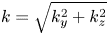 $k = \sqrt { k_{y}^2 + k_{z}^2}$ be the length of the corresponding angular wavevector. Take the power spectral density function
 \begin{equation} \mathcal{P} ( k_{y}, k_{z}) = \begin{cases} \mathcal{P}_o, & \text{if } 1/\lambda_{max}^{*} \leq k/(2 {\rm \pi}) \leq 1/\lambda_{min}^{*}, \\ 0, & \text{otherwise},\end{cases} \end{equation}
where  $\mathcal {P}_o$ is a positive constant taken to be
 $1\ \mathrm {\mu }\textrm {m}^{3}\ \textrm {rad}^{-1}$. Hence,
 $\mathcal {P}$ has units of squared perturbation amplitude per angular wavenumber. Notice that
 $\mathcal {P}$ is non-zero in an annulus of wavevector space, with inner and outer radii corresponding to
 $\lambda _{max}^{*}$ and
 $\lambda _{min}^{*}$, respectively. For each
 $(k_{y,i}, k_{z,j})$ pair for which
 $\mathcal {P}$ is non-zero, define the four coefficients
 \[ \eta^{(1)}_{ij},\quad \eta^{(2)}_{ij},\quad \eta^{(3)}_{ij}\quad \text{and}\quad \eta^{(4)}_{ij} \]
as independent samples drawn from a normal distribution with zero mean and with variance (in  $\mathrm {\mu }\textrm {m}^2$) defined by
 \begin{equation} \mathcal{V} (k_y, k_z)= \frac{ \varDelta k_{y} \varDelta k_{z}}{ 2 {\rm \pi}k} \mathcal{P}( k_y, k_z). \end{equation}
The factor of  $1/k$ in this equation compensates for the larger number of wavevector samples at larger values of
 $k$ (Thornber et al. Reference Thornber2017). Then the noise-perturbation function
 $\delta _x^{*}(y,z)$ is
 \begin{align} \delta_x^{*}( y, z) &= \xi^{*} \sum_{i,j} \left[\eta^{(1)}_{ij} \cos( k_{y,i} y) \cos( k_{z,j} z) + \eta^{(2)}_{ij} \cos( k_{y,i} y) \sin( k_{z,j} z)\right.\nonumber\\ &+ \left.\eta^{(3)}_{ij} \sin( k_{y,i} y) \cos( k_{z,j} z) + \eta^{(4)}_{ij} \sin( k_{y,i} y) \sin( k_{z,j} z) \right], \end{align}
with the summation taken over all available  $\eta ^{(1)}_{ij}, \ldots , \eta ^{(4)}_{ij}$ and where
 $\xi ^{*}$ is a constant dimensionless scaling parameter. The same function
 $\delta _x^{*}$ is used for all simulations, independent of the mesh.
Appendix E. Conventions for Fourier analysis
This appendix summarizes terminology, notation and key equations for Fourier analysis of discrete data sets. The exposition is based on Press et al. (Reference Press, Teukolsky, Vetterling and Flannery1992). To compute discrete Fourier transforms in the present study, we use the routines in the NumPy library (Oliphant Reference Oliphant2006), part of the larger SciPy ecosystem (Jones Reference Jones2001).
Let  $G(y)$ be a real periodic function with period
 $L$. Define a length-
 $N$ sequence of sampled values
 $(G_i)$ by
 \begin{equation} G_i = G( y_i), \quad y_i = i \varDelta, \quad i= 0, 1,\ldots, N-1, \end{equation}
where  $\varDelta = L/N$ is the sampling interval. Assume
 $N$ is even for simplicity. The discrete Fourier transform of
 $(G_i)$ is a sequence of complex numbers
 $(\hat {G}_n)$ defined by
 \begin{equation} \hat{G}_n \equiv \sum_{i=0}^{N-1} G_i \exp \left( 2 {\rm \pi}\ell i n / N \right) \end{equation}
with  $\ell = \sqrt {-1}$. Each
 $\hat {G}_n$ corresponds to a spectroscopic wavenumber
 \begin{equation} f_n = \frac{n}{L}= \frac{n}{N \varDelta}, \quad n = -\frac{N}{2}, \ldots, -1, 0, 1, \ldots, \frac{N}{2}- 1, \end{equation}
which is related to the angular wavenumber  $k_n = 2 {\rm \pi}\,f_n$. The Nyquist wavenumber is
 $1/(2\varDelta )$. From periodicity,
 $\hat {G}_n = \hat {G}_{n+N}$. Also,
 $\hat {G}_n$ is related to an estimate of the continuous Fourier transform
 \begin{equation} \hat{G}(\,f) \equiv \int_{-\infty}^{\infty} G(y) \exp \left( 2 {\rm \pi}\ell f s \right)\,\textrm{d}s \end{equation}
via 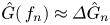 $\hat {G}( \,f_n ) \approx \varDelta \hat {G}_n$. For practical applications, it is common to re-order the sequences
 $(\hat {G}_n)$ in (E2) and
 $(\,f_n)$ in (E3) according to the alternate enumeration
 \begin{equation} (\,f_n) = \frac{1}{L} \left( 0, 1, \ldots, \frac{N}{2}- 2, \frac{N}{2}- 1, -\frac{N}{2}, -\frac{N}{2}+ 1, \ldots, -2, -1 \right), \end{equation}
so that the values of  $n$ in (E2) can be taken as
 $n = 0, \ldots , N-1$. Parseval's theorem is an important property describing the total power in the sequence
 $(G_i)$
 \begin{equation} \sum_{i=0}^{N-1} G_i^2 = \frac{1}{N} \sum_{n=0}^{N-1} |\hat{G}_n|^2. \end{equation}
These concepts extend naturally to two dimensions. Let  $H(y,z)$ be a real periodic function with period
 $L$ in both the
 $y$ and
 $z$ directions. Define the array
 $(H_{ij})$ by
 \begin{equation} H_{ij} = H( y_i, z_j), \quad y_i = i \varDelta, \quad z_j = j \varDelta, \quad i,j= 0, 1,\ldots, N-1. \end{equation}
The 2-D discrete Fourier transform of  $(H_{ij})$ is an array
 $(\hat {H}_{nm})$ defined by
 \begin{equation} \hat{H}_{nm} \equiv \sum_{i=0}^{N-1} \sum_{j=0}^{N-1} H_{ij} \exp \left( 2 {\rm \pi}\ell i n / N \right) \exp \left( 2 {\rm \pi}\ell j m / N \right), \end{equation}
the component corresponding to a spectroscopic wavevector  $(\,f_n, \,f_m)$. The radial power spectral density (RPSD)
 $\mathcal {D}_{H}(\,f)$ of
 $H$ can be approximated via
 $\mathcal {D}_{H}( \,f_q) \approx \mathcal {D}_{H,q}$, where
 \begin{equation} \left. \begin{gathered} \mathcal{D}_{H,q} \equiv \frac{ L}{N^4} \sum_{ n,m \in \beta(\, f_q) } \left| \hat{H}_{nm} \right|^2,\\ \beta(\,f_q ) = \left\{ n,m : \,f_q - \frac{\varpi}{2} \leq \,\sqrt{ f_n^2 + \,f_m^2} < \,f_q + \frac{\varpi}{2} \right\}. \end{gathered} \right\} \end{equation}
Here,  $(\,f_q)$ is a sequence of spectroscopic wavevector magnitudes, with
 $\varpi \equiv \,f_{q+1}- \,f_q = 1/L$ as in (E3) and (E5). The quantity
 $\mathcal {D}_{H,\,q}$ gives a measure of how much power in
 $(H_{ij})$ falls within a wavevector-magnitude bin centred at
 $f_q$ with bin width
 $\varpi$, and
 $\beta (\,f_q)$ is the collection of
 $(n,m)$ pairs that correspond to that bin. The multiplicative factor
 $L/N^4= \varDelta ^4/L^3$ ensures that
 \begin{equation} \int \mathcal{D}_H(\,f)\,\textrm{d}f \approx \sum_q \mathcal{D}_{H,\,q} \varpi = \sum_{i=0}^{N-1} \sum_{j=0}^{N-1} \frac{H_{ij}^2}{N^2} \approx \frac{1}{L^2} \int_{0}^{L} \int_{0}^{L} H^2( y, z) \,{\textrm{d} y}\,\textrm{d}z, \end{equation}
which can be verified using the 2-D analogue of (E6). If  $H$ has units of
 $V$ and
 $y$ and
 $z$ each have units of
 $W$, then
 $\mathcal {D}_H$ has units of
 $V^2 W$.
Now consider a 2-D slice through a 3-D flow field, with periodic boundary conditions on the slice. Building on the conventions in the previous paragraph, let  $( u_{1}'', u_{2}'', u_{3}'' )_{ij}$ be a discrete sample of the velocity Favre-fluctuation vector
 $( u_{1}'', u_{2}'', u_{3}'')$. The turbulent energy spectrum
 $\mathcal {R}(\,f)$ can be approximated via
 $\mathcal {R}(\,f_q) \approx \mathcal {R}_{q}$, where
 \begin{equation} \mathcal{R}_{q} \equiv \frac{ L}{2 N^4} \sum_{ n,m \in \beta( \,f_q) } \left[ \left|\widehat{u_{1}''}_{nm}\right|^2 + \left|\widehat{u_{2}''}_{nm}\right|^2 + \left|\widehat{u_{3}''}_{nm}\right|^2 \right] \end{equation}
with  $\beta (\,f_q)$ defined as in (E9). As in (E10), observe that
 $\int \mathcal {R}\,\textrm {d}f \approx \sum \mathcal {R}_q \varpi = \sum \sum \mathcal {I}_{ij}/ N^2 \approx \overline {\mathcal {I}}$, where
 $\mathcal {I}$ is the LTKE from (4.4). We find that the method represented by (E11) is consistent with the shell-averaging method of Ishida, Davidson & Kaneda (Reference Ishida, Davidson and Kaneda2006, appendix B), after adapting the latter for 2-D analysis; method-to-method differences in
 $\mathcal {R}$ at the mixing-layer centre-plane are somewhat more appreciable at pre-reshock times, when the flow is strongly anisotropic, than at post-reshock times. See Pope (Reference Pope2000, § 6.5) and Davidson (Reference Davidson2015, § 8.1.4) for detailed discussions of
 $\mathcal {R}$ and its importance.
Appendix F. MDTKE analysis: additional details
Expanding on the analysis in § 4.4, an evolution equation for  $\mathcal{K}$ can be derived from the Navier–Stokes equations (3.3)
 \begin{align} \frac{ \partial}{ \partial t} \left( \mathcal{K} \right) + \frac{ \partial}{ \partial x_j} \left( \mathcal{K} \widetilde{u}_j \right) &= \underbrace{\left( - \overline{ \rho u_i'' u_j''} \frac{ \partial \widetilde{u}_i}{\partial x_j} \right)}_{ \mathbb{T}_{I}} + \underbrace{\left( \overline{u_i''} \left[ \frac{ \partial \bar{\sigma}_{ij} }{ \partial x_j} - \frac{ \partial \bar{p} }{ \partial x_i} \right] \right)}_{ \mathbb{T}_{II}} + \underbrace{\left( \overline{p' \frac{ \partial u_i'' }{ \partial x_i}}\, \right)}_{ \mathbb{T}_{III}}\nonumber\\ &\quad + \underbrace{\left( -\frac{ \partial}{ \partial x_j} \left[ \tfrac{1}{2} \bar{\rho} \widetilde{ \left( u_i'' u_i'' u_j'' \right)} + \overline{ p' u_j''} - \overline{ \sigma_{ij}' u_i''} \right] \right)}_{ \mathbb{T}_{IV}} + \underbrace{\left( -\overline{ \sigma_{ij}' \frac{ \partial u_i''}{ \partial x_j} } \right)}_{ \mathbb{T}_{V}} . \end{align}
This equation is central to the construction of reduced-order Reynolds-averaged Navier–Stokes models. As explained in Sagaut & Cambon (Reference Sagaut and Cambon2008) and Chassaing et al. (Reference Chassaing, Antonia, Anselmet, Joly and Sarkar2010), the first term  $\mathbb {T}_{I}$ is the shear production term, which is zero when the mean rate of strain
 $(\partial \widetilde {u}_i/\partial x_j + \partial \widetilde {u}_j/\partial x_i)/2$ is zero. The second term
 $\mathbb {T}_{II}$ is the turbulent-mass-flux coupling term, so named because the product of density and
 $\overline {u_i''}= \overline {u}_i- \widetilde {u}_i$ can be interpreted as a turbulent mass flux that vanishes for a constant-density flow. As a contribution to
 $\mathbb {T}_{II}$, the product
 $-\,\overline {u_i''}\,\partial \overline {p}/\partial x_i$ is called the buoyancy production term (Schilling & Latini Reference Schilling and Latini2010; Thornber et al. Reference Thornber, Griffond, Bigdelou, Boureima, Ramaprabhu, Schilling and Williams2019) or the mean pressure work term (Chassaing et al. Reference Chassaing, Antonia, Anselmet, Joly and Sarkar2010). The third term
 $\mathbb {T}_{III}$ is the pressure–dilatation term. The fourth term
 $\mathbb {T}_{IV}$ is the turbulent transport term, which vanishes for a homogeneous flow. The fifth term
 $\mathbb {T}_{V}$ is the dilatational dissipation term. The shear production term is associated with exchange between the turbulent kinetic energy and mean-flow kinetic energy, while the pressure–dilatation and dilatational dissipation terms are associated with exchange between the turbulent kinetic energy and mean-flow internal energy. The turbulent transport term is associated with spatial redistribution of turbulent kinetic energy. In the present study, the terms on the right-hand side of (F1) can be calculated (as functions of
 $x$ and
 $t$) using the Reynolds-averaging operator (3.19). The supplementary material provides a complete derivation of (F1) and elaborates on some computational issues associated with it.
Figure 21 plots normalized mixing-layer integrals of each term  $\mathbb {T}_{I}, \ldots , \mathbb {T}_{V}$ versus time, in the finest-resolution baseline simulation. Figure 21(a) shows that, before reshock, MDTKE production is principally due to the turbulent-mass-flux coupling term
 $\mathbb {T}_{II}$ as the
 $\mathbb {M}_H$–
 $\mathbb {M}_L$ interface moves downstream and instabilities grow. The buoyancy production term accounts for nearly all of
 $\mathbb {T}_{II}$ at these times. The
 $\mathbb {T}_{I}$ term accounts for some MDTKE destruction after first shock, while the other three terms do not contribute significantly to the net balance of MDTKE. The persistent generation of MDTKE via buoyancy production mirrors the persistent generation of enstrophy via the baroclinic source term in (4.14); see figure 14(b). Both trends are consistent with RT instability growth throughout the post-first-shock, pre-reshock interval, with sustained deceleration of the heavy–light mixing layer. As discussed in § 4.3, the flows simulated here cannot be accurately characterized as either ‘pure RM’ or ‘pure RT’.
Evolution of the mixing-layer integrals of each term  $\mathbb {T}_{I}, \ldots , \mathbb {T}_{V}$ in (F1), normalized by
 $\lfloor { \mathcal {K}} \rfloor$, in the finest-resolution baseline simulation: (a) displays early-time results before reshock, and (b) displays late-time results after reshock. Note the difference in the ordinate limits of the two figures. Equation (3.22) defines the mixing-layer integral.

Figure 21(b) shows that MDTKE production during reshock traversal of the mixing layer is principally due to the shear production term  $\mathbb {T}_{I}$, with the component
 $-\overline {\rho u_1'' u_1''} \partial \widetilde {u}_1/\partial x_1$ being the dominant contributor to
 $\mathbb {T}_{I}$. During reshock traversal, the pressure–dilatation term
 $\mathbb {T}_{III}$ contributes significantly to MDTKE production, and the turbulent-mass-flux coupling term
 $\mathbb {T}_{II}$ is responsible for some MDTKE destruction.
Figure 22 plots instantaneous, normalized profiles of the five terms in the finest-resolution baseline simulation at two pre-reshock and two post-reshock times. Figures 22(a) and 22(b) correspond to moderate and late pre-reshock times, respectively, and they support the claims made in the previous paragraph. The turbulent-mass-flux coupling term  $\mathbb {T}_{II}$ dominates MDTKE production. The turbulent transport term
 $\mathbb {T}_{IV}$ is non-zero across most of the mixing layer, although the magnitude of its integral is small. Figure 22(c) indicates that – as the mixing layer expands rapidly after reshock – MDTKE destruction occurs due to both
 $\mathbb {T}_{I}$ and
 $\mathbb {T}_{II}$, and spatial redistribution due to
 $\mathbb {T}_{IV}$ is significant. Figure 22(d) suggests an approximate balance between
 $\mathbb {T}_{II}$ and
 $\mathbb {T}_{IV}$ near the time of maximum mixing-layer width. At all times, losses due to the dilatational dissipation term
 $\mathbb {T}_{V}$ are relatively minute.
Instantaneous profiles of each term  $\mathbb {T}_{I}, \ldots , \mathbb {T}_{V}$ in (F1), normalized by
 $\lfloor { \mathcal {K}} \rfloor$, in the finest-resolution baseline simulation at (a) 20 ns, (b) 30 ns, (c) 35 ns and (d) 45 ns. The profiles are plotted as functions of the dimensionless mixing-layer position
 $(x- x_c)/x_w$, where
 $x_c$ is the mixing-layer centre-plane and
 $x_w$ is the mixing-layer fitting width; see (4.3). In each figure, two solid vertical lines denote the bubble front
 $x_b$ and spike front
 $x_s$ as defined in § 3.5. Note that the ordinate limits vary across the four figures. Equation (3.22) defines the mixing-layer integral.

The qualitative trends described in the preceding three paragraphs are also seen in the two lower-resolution baseline simulations and in all three CPVs, suggesting that the trends are physically meaningful and not merely numerical artefacts. The supplementary material provides results, corresponding to figure 21, from the two lower-resolution baseline simulations. As in the discussion of enstrophy evolution in § 4.6, it is important to emphasize that (F1) is not exact for an under-resolved 3-D simulation. Numerical truncation errors associated with MDTKE evolution were recently analysed by Thornber et al. (Reference Thornber, Griffond, Bigdelou, Boureima, Ramaprabhu, Schilling and Williams2019). Although beyond the scope of the present study, further analysis of numerical errors is warranted. In particular, numerical dissipation likely has a role in the post-reshock MDTKE decay.