



1. Introduction
Viscoelastic fluids subject to a shearing flow often exhibit strikingly novel instabilities engendered by their elastic nature, which are absent in their Newtonian counterparts. For instance, it is well known, since the pioneering work of Larson et al. (Reference Larson, Shaqfeh and Muller1990), that Taylor–Couette flow of a viscoelastic fluid exhibits a linear instability even when fluid inertia is negligible. Analogous instabilities have been demonstrated for the flow of polymer solutions in other curvilinear geometries such as cone-and-plate flow (McKinley et al. Reference McKinley, Byars, Brown and Armstrong1991), torsional flow between parallel circular discs (Byars et al. Reference Byars, Oztekin, Brown and McKinley1994), and the Dean and Taylor–Dean flow configurations (Joo & Shaqfeh Reference Joo and Shaqfeh1991, Reference Joo and Shaqfeh1992, Reference Joo and Shaqfeh1994). These instabilities, collectively referred to as ‘purely elastic’ instabilities (see Shaqfeh Reference Shaqfeh1996), rely on two key ingredients in the base state – streamline curvature and a streamwise normal stress that has a tensile character (owing to stretched polymers). The latter results in a ‘hoop stress’ in the aforementioned curvilinear flows that then drives an instability even in the absence of inertial forces; the latter forces come into play even in a Newtonian fluid, leading to inertial instabilities beyond a threshold Reynolds number (
 $\textit{Re}$
) in the aforementioned configurations. The Pakdel–McKinley (PM) scaling arguments (McKinley et al. Reference McKinley, Pakdel and Oztekin1996; Pakdel & McKinley Reference Pakdel and McKinley1996) provide a unifying expression for the onset of hoop-stress-driven instabilities, given by
 \begin{equation} \frac {\lambda V}{\mathcal{R}} \frac {N_1}{|\tau |} \geqslant M_{\textit{crit}}^2 , \end{equation}
where
 $\lambda$
is the (longest) relaxation time of the fluid,
 $V$
is a characteristic velocity scale,
 $\mathcal{R}$
is the pertinent radius of curvature,
 $N_1$
is the first normal stress difference,
 $\tau$
is the total shear stress in the base-state and
 $M_{\textit{crit}}$
is an
 $O(1)$
number sensitive to the actual geometry.
The PM criterion cannot be satisfied for rectilinear shearing flows (with
 $\mathcal{R} \rightarrow \infty$
), implying that hoop-stress-driven linear instabilities are absent in such flows. Hoop stresses in these flows can, however, become relevant at a nonlinear order, owing to curvature of the perturbed streamlines, as has been demonstrated within the framework of a weakly nonlinear stability analysis (Morozov & van Saarloos Reference Morozov and van Saarloos2005a
, Reference Morozov and van Saarloos2007, Reference Morozov and van Saarloos2019). The above-mentioned absence of a hoop-stress-driven linear instability had led to the viewpoint that purely elastic instabilities are restricted to curvilinear configurations, even if they are more complicated than the aforementioned canonical geometries (Haward et al. Reference Haward, McKinley and Shen2016), and that rectilinear viscoelastic shear flows are therefore linearly stable (Bertola et al. Reference Bertola, Meulenbroek, Wagner, Storm, Morozov, van Saarloos and Bonn2003; Pan et al. Reference Pan, Morozov, Wagner and Arratia2013).
In a significant departure from this paradigm, recent work by Khalid et al. (Reference Khalid, Shankar and Subramanian2021b
) demonstrated that inertialess plane Poiseuille flow of an Oldroyd-B fluid is linearly unstable in the limit of high Weissenberg numbers (
 $\textit{Wi} = \lambda V/H \sim 10^3$
,
 $V$
being the base-state maximum speed and
 $H$
the channel half-width) and a near-unity solvent to solution viscosity ratio (
 $\beta \gt 0.99)$
; this corresponds to ultra-dilute highly elastic polymer solutions. The unstable mode has a phase speed close to the base-state maximum, belonging therefore to a class of ‘centre modes’, and the instability arises due to a critical-layer mechanism that does not rely on streamline curvature. Khalid et al. (Reference Khalid, Shankar and Subramanian2021b
) further showed that, with increasing
 $\textit{Re}$
, the elastic centre-mode instability smoothly crosses over to the elastoinertial centre-mode instability, predicted in an earlier effort by Khalid et al. (Reference Khalid, Chaudhary, Garg, Shankar and Subramanian2021a
). Although a connection between the elastoinertial and elastic turbulent states was first speculated by Samanta et al. (Reference Samanta, Dubief, Holzner, Schäfer, Morozov, Wagner and Hof2013) in their observations concerning the onset of elastoinertial turbulence in pipe flow of polymer solutions, the effort of Khalid et al. (Reference Khalid, Shankar and Subramanian2021b
) for plane Poiseuille flow provided a rigorous demonstration of a connected linearly unstable region, across the elastoinertial range, and extending down to the inertialess limit. Kerswell & Page (Reference Kerswell and Page2024) have recently carried out a matched asymptotic expansions analysis to capture this unstable centre mode. Further, Buza et al. (Reference Buza, Page and Kerswell2022b
) and subsequently Khalid et al. (Reference Khalid, Badoni, Dutta, Naidu, Subramanian and Shankar2025) have shown using the FENE-P model, which accounts for finite extensibility of the polymer molecules, that the elastic centre-mode instability is present even for
 $\textit{Wi} \sim O(100)$
and
 $\beta \approx 0.97$
. Thus, use of the more realistic FENE-P model extends the unstable domain to experimentally accessible parts of the parameter space.
Recent efforts have identified an unstable centre mode in other rectilinear shearing flows as well. Yadav et al. (Reference Yadav, Subramanian and Shankar2024) have shown that the elastic centre-mode instability is present in the Couette–Poiseuille family (CPF), but only when the base-state velocity profile is non-monotonic, with a maximum within the flow domain; the instability being absent in plane Couette flow and, more generally, in shearing flows with monotonic velocity profiles. This intimate connection between the presence of a base-state maximum and the existence of a centre-mode instability is further corroborated by the presence of the latter in viscoelastic Kolmogorov flow (Kerswell & Page Reference Kerswell and Page2024; Lewy & Kerswell Reference Lewy and Kerswell2025); although the significance of this finding was not recognised in the original analysis of Boffetta et al. (Reference Boffetta, Celani, Mazzino, Puliafito and Vergassola2005). An analogue of the centre-mode instability was also shown to be present in viscoelastic film flow down an inclined plane (Priyadarshi et al. Reference Priyadarshi, Srita, Bhaskar, Khalid, Subramanian and Shankar2023), with a semi-parabolic base-state velocity profile.
Thus, there are two qualitatively different elastic instabilities that operate in viscoelastic shearing flows: (i) the hoop-stress mode (‘HSM’ henceforth), which requires the presence of streamline curvature, but exists even for monotonic velocity profiles (such as Taylor–Couette flow); and (ii) the elastic centre mode (‘CM’ henceforth), which does not rely on streamline curvature, but requires a non-monotonic base-state velocity profile. This raises the intriguing possibility that these modes might co-exist in flow configurations possessing both the aforementioned ingredients. That is to say, one has the potential for elastic instabilities of different physical origins in the same flow, a possibility that has not yet been explored in the literature. One such configuration is Dean flow – the flow in a curved channel driven by an azimuthal pressure gradient. In the Newtonian context, this configuration was first analysed by Dean & Chapman (Reference Dean and Chapman1928), who showed the presence of a centrifugal instability. The threshold for this instability, in the narrow-gap limit, can be obtained from an inertial analogue of the above-mentioned PM criterion, with the Reynolds number
 $\textit{Re}$
replacing
 $\textit{Wi}$
; this was indeed pointed out by McKinley et al. (Reference McKinley, Pakdel and Oztekin1996) while formulating their criterion for elastic instabilities. As alluded to already, Joo & Shaqfeh (Reference Joo and Shaqfeh1991, Reference Joo and Shaqfeh1992, Reference Joo and Shaqfeh1994) analysed the viscoelastic Dean flow problem, albeit in the inertialess limit (
 $\textit{Re} = 0$
), and showed the presence of an HSM instability in this configuration. One could also have a combination of an azimuthal pressure gradient and wall motion driving the flow, the resulting configuration being dubbed the ‘Taylor–Dean’ flow (Joo & Shaqfeh Reference Joo and Shaqfeh1991) and being more easily realised in experiments.
We carry out a linear stability analysis of viscoelastic Dean flow to explore the relevance of both centre- and hoop-stress modes in a parameter space comprising
 $\textit{Wi}$
,
 $\beta$
, and the gap-width ratio
 $\epsilon = d/\mathcal{R}$
,
 $d$
being the channel width. For the case where the curved channel is the gap between concentric rotating cylinders with
 $R_2$
and
 $R_1$
being the outer and inner cylinder radii, as is typically the case in experiments,
 $d= (R_2 - R_1)$
may be identified with the gap width, and the radius of curvature with
 $R_1$
. We consider the inertialess regime in this effort and, therefore, set
 $\textit{Re} = 0$
. Traditionally, the HSM was first analysed in the narrow-gap limit (Larson et al. Reference Larson, Shaqfeh and Muller1990; Joo & Shaqfeh Reference Joo and Shaqfeh1991), corresponding to
 $\epsilon \ll 1$
, with this assumption being relaxed in subsequent numerical investigations (Joo & Shaqfeh Reference Joo and Shaqfeh1992, Reference Joo and Shaqfeh1994). In the narrow-gap limit, for the hoop stress to remain relevant in the leading order radial momentum balance, one requires
 $\epsilon ^{1/2} \textit{Wi} \sim O(1)$
. Here,
 $\textit{Wi} = \lambda U_m/d$
is the Weissenberg number based on the gap width
 $d$
and a velocity scale
 $U_m$
associated with the Dean flow profile (defined later). Thus, in the narrow-gap limit, the critical
 $\textit{Wi}$
for the HSM instability must diverge as
 $\epsilon ^{-1/2}$
. In the same limit, the critical
 $\textit{Wi}$
for the CM instability is independent of
 $\epsilon$
and approaches that of plane Poiseuille flow (Khalid et al. Reference Khalid, Chaudhary, Garg, Shankar and Subramanian2021a
). At a scaling level, therefore, as
 $\epsilon \rightarrow 0$
, the critical
 $\textit{Wi}$
for HSM should eventually become larger than that for the CM. However, owing to the relatively large threshold,
 $\textit{Wi} \sim O(10^3)$
for the CM (within the Oldroyd-B framework), it is necessary to carry out a stability analysis to determine the precise value of
 $\epsilon$
corresponding to this cross-over, and thereby assess its relevance to typical configurations used in experiments and applications. To this end, we present here a comprehensive account of the parameter regimes in which either of the aforementioned modes is the most unstable in viscoelastic Dean flow, by considering arbitrary gap-width ratios (
 $\epsilon$
), and by including both axisymmetric and non-axisymmetric disturbances.
Of particular relevance to the present effort is the recent preprint of Lu & Hof (Reference Lu and Hof2026) that reports experimental observations of instabilities in pressure-driven flow of polymer solutions through curved (helical) pipes; the curvature parameter here is
 $d/R$
(ratio of pipe diameter to helical coil radius), and is the analogue of
 $\epsilon$
defined earlier. The authors find a CM instability in the limit
 $d/R \ll 1$
, this being consistent with the earlier results of Choueiri et al. (Reference Choueiri, Lopez, Varshney, Sankar and Hof2021) for straight pipes. The threshold
 $\textit{Wi}$
for the instability remains insensitive to increasing curvature until
 $d/R \approx 0.06$
, beyond which there is a cross-over to an HSM, characterised by a threshold
 $\textit{Wi}$
that decreases with further increase in
 $d/R$
. Interestingly, Lu & Hof (Reference Lu and Hof2026) show that the HSM continues to exist for
 $d/R \lt 0.06$
, albeit as a secondary instability, occurring at a
 $\textit{Wi}$
higher than the CM threshold. In § 6, we show that the aforementioned picture is broadly consistent with our findings for the Dean flow configuration, and also expand on the nature of secondary transitions in both curved channel and pipe configurations.
While the existence of two types of elastic instabilities in the Dean flow configuration is of interest from the fundamental viewpoint, it is also significant from the applications perspective. Viscoelastic Dean flow is often used for hydrodynamic focusing of particles in curved (Nikdoost & Rezai Reference Nikdoost and Rezai2020), spiral (Bai et al. Reference Bai, Zhang, Wei, Wang, Du, Wang, Chen and Wang2023) and serpentine (Chen et al. Reference Chen, Huang, Ni and Xiang2024) microchannels. Although such experiments involve finite Reynolds numbers, the secondary flows emerging from the elastic instabilities reported in this study could certainly impact particle migration and, more generally, the efficiency of focussing protocols on microfluidic platforms. Polymer solutions are also used as displacing agents in enhanced oil recovery to remove capillary entrapments of oil in the pores. In this context, flow in serpentine microfluidic channels has been used to mimic the tortuous nature of the flow in porous media (Shakeri et al. Reference Shakeri, Jung and Seemann2021), wherein elastic instabilities are harnessed in triggering the breakup of large capillary entrapments and in the eventual removal of the same. Importantly, the elastic turbulence regime accessed in previous experiments involving serpentine microchannels (also regarded as an important means of achieving efficient mixing in microfluidic devices; see Groisman & Steinberg Reference Groisman and Steinberg2001, Reference Groisman and Steinberg2004) is either explicitly or implicitly understood as the eventual consequence of an initial hoop-stress-driven instability. Our findings suggest that there might exist two distinct pathways (viz., an HSM-based route and a CM-based route, as suggested by the title) to the eventual turbulent regime and, perhaps, even two different kinds of turbulent states, depending on the wavelength of modulation of the serpentine channel.
We consider both the Oldroyd-B and FENE-P constitutive equations to model the viscoelastic fluid. The Oldroyd-B model has the necessary ingredients to capture both the HSM and CM, but owing to its prediction of a shear-rate-independent viscosity and first normal stress coefficient, it may be not accurate for fast shearing flows of polymer solutions (translating to a large threshold
 $\textit{Wi}$
for the CM in the present context) where shear thinning becomes important. This lacuna is due to the restrictive assumption of the polymer molecule being an infinitely extensible bead-spring dumbbell. The FENE-P model (Bird et al. Reference Bird, Dotson and Johnson1980) overcomes this shortcoming by accounting for finite extensibility via the parameter
 $L$
, the ratio of the fully extended length of the polymer (dumbbell) to its equilibrium size; the Oldroyd-B model being realised in the limit
 $L \rightarrow \infty$
. The FENE-P model predicts shear thinning of both the viscosity and the first normal stress coefficient, and hence is a more realistic model at higher
 $\textit{Wi}$
. As will be shown later, consideration of finite extensibility is particularly important in the present scenario, on account of its contrasting effects on the HSM and CM instabilities. Well, why then should one consider the Oldroyd-B model at all? As noted by Shaqfeh & Khomami (Reference Shaqfeh and Khomami2021), in their review article commemorating the birth centenary of James Oldroyd, the results obtained using the Oldroyd-B fluid have their own value in terms of providing a base reference, and (we quote) ‘it is perilous…to ignore the analysis based on the Oldroyd-B model for any elastic flow problem’! We examine both axisymmetric and non-axisymmetric disturbances in the narrow-gap limit (
 $\epsilon \ll 1$
), and for finite gap-width ratios (
 $\epsilon \sim O(1)$
). The consideration of non-axisymmetric disturbances gains relevance because, while the HSM is present for axisymmetric disturbances, the CM is present even for two-dimensional disturbances. Even for the HSM, a non-zero azimuthal wavenumber can lead to a slight destabilisation in certain cases, as has been shown by Avgousti & Beris (Reference Avgousti and Beris1993) for viscoelastic Taylor–Couette flow.
The rest of this paper is organised as follows. The governing equations for both Oldroyd-B and FENE-P models are discussed in § 2.1. The base state velocity and stresses are discussed in § 2.2 for the Oldroyd-B model and in § 2.3 for the FENE-P model. The linearisation procedure is briefly introduced in § 2.4, with Appendices A and B providing the full system of linearised equations governing small amplitude disturbances in the respective cases. Since earlier efforts examining the Dean flow configuration have solely focused on the unstable modes, we begin here by discussing the nature of the complete elastic eigenspectrum for Dean flow of both Oldroyd-B and FENE-P fluids in § 3, with additional details of representative eigenspectra provided in Appendix C; §§ 3.1 and 3.2 discuss the eigenspectra for the axisymmetric and non-axisymmetric cases, respectively. We then discuss the CM instability in viscoelastic Dean flow in § 4. Herein, we first use the Oldroyd-B model in § 4.1 to map out the unstable parameter regimes for arbitrary
 $\epsilon$
, both for two- and three-dimensional perturbations, and then proceed to examine the role of finite extensibility (using the FENE-P model) in § 4.2. Section 5 begins with a brief recap of the key results for HSM within the Oldroyd-B framework, following which we examine the role of finite extensibility on the HSM for both axisymmetric (§ 5.1) and non-axisymmetric (§ 5.2) disturbances. Appendix D provides a brief compilation of eigenfunctions for the relevant unstable modes. Finally, § 6 provides a brief summary of the salient conclusions emerging from this effort, along with discussions on connection to experimental studies and on the various possible transition pathways in elastic Dean flow.
Non-dimensionalisation scheme adopted in this study. Most symbols are defined in the text. Here,
 $H_{s\!p}$
is the equilibrium spring constant in the Oldroyd-B and FENE-P models,
 $k_B$
is the Boltzmann constant, and
 $T$
is the absolute temperature.

Table 1. Long description
The table presents a non-dimensionalisation scheme with four columns: Parameter, Dimensional variable, Scale, and Dimensionless variable. It has eight rows, each corresponding to a different parameter: Length, Velocity, Time, Pressure, Polymeric stress, Disturbance frequency, and Conformation tensor. Row 1: Parameter, Length; Dimensional variable, r*; Scale, d (gap width); Dimensionless variable, r. Row 2: Parameter, Velocity; Dimensional variable, v*; Scale, Um (average velocity); Dimensionless variable, v. Row 3: Parameter, Time; Dimensional variable, t*; Scale, d/Um; Dimensionless variable, t. Row 4: Parameter, Pressure; Dimensional variable, p*; Scale, ηUm/d; Dimensionless variable, p. Row 5: Parameter, Polymeric stress; Dimensional variable, τ*; Scale, ηpUm/d; Dimensionless variable, τ. Row 6: Parameter, Disturbance frequency; Dimensional variable, ω*; Scale, λ (relaxation time); Dimensionless variable, ω. Row 7: Parameter, Conformation tensor; Dimensional variable, C*; Scale, kBT/Hsp; Dimensionless variable, C.
Schematic of the geometry and the coordinate system considered.

2. Problem formulation and numerical method
2.1. Governing equations
We consider steady, fully developed pressure-driven flow of a viscoelastic fluid between concentric cylindrical surfaces with radii
 $R_1$
and
 $R_2$
(
 $R_1 \lt R_2$
), corresponding to a gap width
 $d = R_2 - R_1$
; the gap-width ratio is defined as
 $\epsilon = d/R_1$
. A cylindrical coordinate system with
 $r$
,
 $\theta$
,
 $z$
denoting the radial, azimuthal and axial coordinates, respectively, shown in figure 1, is used with the pressure gradient imposed along the azimuth. The scales used for rendering dimensionless the physical quantities, associated with both Oldroyd-B and FENE-P models, are summarised in table 1. The dimensionless continuity and inertialess Cauchy momentum equations take the form
 \begin{equation} \boldsymbol{\nabla }\boldsymbol{\cdot }\boldsymbol{v}=0 , \end{equation}
 \begin{equation} 0 =-\boldsymbol{\nabla }\!{p}+ {\beta } \,{\nabla} ^2 \, \boldsymbol{v} + {(1-\beta )} \, \boldsymbol{\nabla }\boldsymbol{\cdot }\boldsymbol{\tau } , \end{equation}
with
 $\boldsymbol{v}$
and
 $p$
being the velocity and pressure fields, and
 $\boldsymbol{\tau }$
the polymeric stress tensor. In (2.2),
 $\beta = \eta _s/\eta$
is the solvent to solution viscosity ratio, where
 $\eta = \eta _s + \eta _p$
is the total (zero-shear) solution viscosity with
 $\eta _p$
and
 $\eta _s$
being the zero-shear polymer and solvent viscosities, respectively.
In the Oldroyd-B model (Larson Reference Larson1988), the polymer solution is modelled as a non-interacting suspension of Hookean dumbbells and the polymeric stress
 $\boldsymbol{\tau }$
is governed by
 \begin{eqnarray} \boldsymbol{\tau }+\textit{Wi} \left(\frac {\partial \boldsymbol{\tau }}{\partial t}+ \boldsymbol{v}\boldsymbol{\cdot }\boldsymbol{\nabla }\boldsymbol{\tau }-\boldsymbol{\nabla }\boldsymbol{v}^\intercal \boldsymbol{\cdot }\boldsymbol{\tau }- \,\boldsymbol{\tau }\boldsymbol{\cdot }\boldsymbol{\nabla }\boldsymbol{v} \right)= \big (\boldsymbol{\nabla }\boldsymbol{v}+\boldsymbol{\nabla }\boldsymbol{v}^\intercal \big ). \end{eqnarray}
Here,
 $\textit{Wi} = \lambda U_m/d$
is the Weissenberg number. In the FENE-P model, the dumbbells are finitely extensible and the polymeric contribution to the stress tensor is given by
 \begin{equation} \boldsymbol{\tau } = \frac {f \boldsymbol{C} - \boldsymbol{I}}{\textit{Wi}}. \end{equation}
Here,
 $\boldsymbol{C}$
denotes the dimensionless conformation tensor, while
 $\boldsymbol{I}$
is the identity tensor representing the isotropic distribution of dumbbell conformations in the absence of an imposed flow. The Peterlin closure function
 $f$
(Bird et al. Reference Bird, Dotson and Johnson1980; Herrchen & Ottinger Reference Herrchen and Ottinger1997) is defined as
 \begin{equation} f = \frac {L^2 - 3}{L^2 -tr(\boldsymbol{C})}, \end{equation}
where
 $L$
represents the dimensionless extensibility parameter, de’s maximum extension to its equilibrium root-mean-square value; the Oldroyd-B model being attained in the limit of infinite extensibility viz.,
 $L \rightarrow \infty$
, when
 $f \rightarrow 1$
. The conformation tensor is governed by the following evolution equation:
 \begin{equation} \frac {\partial \boldsymbol{C}}{\partial t}+ \boldsymbol{v}\boldsymbol{\cdot }\boldsymbol{\nabla }\boldsymbol{C}-\boldsymbol{\nabla }\boldsymbol{v}^\intercal \boldsymbol{\cdot }\boldsymbol{C}- \,\boldsymbol{C}\boldsymbol{\cdot }\boldsymbol{\nabla }\boldsymbol{v} = -\boldsymbol{\tau }. \end{equation}
No-slip boundary conditions at the inner and outer cylinder walls apply to all velocity components. Since stress diffusion is neglected in the constitutive equations, no boundary conditions need be specified for either the polymeric stress or conformation tensors.
2.2. Base state for the Oldroyd-B Model
The base state velocity profile for Dean flow of an Oldroyd-B fluid is identical to its Newtonian counterpart (Diprima Reference Diprima1959; Joo & Shaqfeh Reference Joo and Shaqfeh1992) and, therefore, independent of
 $\textit{Wi}$
. The non-dimensional velocity profile, after using the coordinate transformation
 $r^{*} = R_1(1 + \epsilon y)$
, is given by
 \begin{equation} \overline {\boldsymbol{v}} = \left [\!\begin{array}{ccccc} \overline v_{r} \\[3pt] \overline v_{\theta } \\[3pt] \overline v_{z} \\ \end{array}\!\right ] = \left [\!\begin{array}{ccccc} 0 \\[3pt] U(y) \\[3pt] 0 \\ \end{array}\!\right ] \!, \end{equation}
 \begin{equation} U(y) = \frac { -K \left [ (1 + \epsilon y) - \frac {1}{(1 + \epsilon y)}\right ] + \left [(1 + \epsilon y) \ln (1 + \epsilon y) \right ] }{K \left [\frac { \ln (1 + \epsilon )}{\epsilon }\right ] - \frac {1}{4} (2 + \epsilon )} , \end{equation}
where
 $K = {(1 + \epsilon )^2 \ln (1+ \epsilon )}/{(1 + \epsilon )^2 - 1}$
and the average velocity that has been used as the scale in (2.8) is given by
 $U_m = ( {( {\partial p}/{\partial \theta }) R_1}/{2 \eta }) (K [ { \ln (1 + \epsilon )}/{\epsilon } ] - ({1}/{4}) (2 + \epsilon ) )$
. The polymer contribution to the base state stress tensor is given by
 \begin{equation} \boldsymbol{\overline \tau } = \left [\!\!\begin{array}{ccccc} \overline \tau _{rr} & \overline \tau _{r \theta } & \overline \tau _{rz} & \\[3pt] \overline \tau _{\theta r} & \overline \tau _{\theta \theta } & \overline \tau _{\theta z} & \\[3pt] \overline \tau _{zr } & \overline \tau _{z \theta } & \overline \tau _{zz} & \\ \end{array}\!\!\!\!\!\right ] = \left [\!\begin{array}{ccccc} 0 & U' - \frac {\epsilon }{1 + \epsilon y}U & 0 & \\[11pt] U' - \frac {\epsilon }{1 + \epsilon y}U & 2 \textit{Wi} \left(U' - \frac {\epsilon }{1 + \epsilon y}U\right)^2 & 0 & \\[11pt] 0 & 0 & 0 & \\ \end{array}\!\!\right ] \!, \end{equation}
where
 $ \zeta ' \equiv D\zeta \equiv{{\rm d}\zeta }/{{\rm d}y}$
.
2.3. Base state for the FENE-P model
The base state velocity field, conformation tensor and the polymer stress tensor in this case are given by
 \begin{equation} \overline {\boldsymbol{v}} = \left [\! \begin{array}{ccccc} \overline v_{r} \\[3pt] \overline v_{\theta } \\[3pt] \overline v_{z} \\ \end{array} \!\right ] = \left [\! \begin{array}{ccccc} 0 \\[3pt] U(y) \\[3pt] 0 \\ \end{array}\!\right ] \!, \end{equation}
 \begin{equation} \boldsymbol{\overline C} = \left [\!\! \begin{array}{ccccc} \overline C_{rr} & \overline C_{r\theta } & \overline C_{rz} & \\[5pt] \overline C_{\theta r} & \overline C_{\theta \theta } & \overline C_{\theta z} & \\[5pt] \overline C_{zr} & \overline C_{z\theta } & \overline C_{zz} & \\ \end{array}\!\!\!\!\!\!\right ] = \left [\! \begin{array}{ccccc} \frac {1}{\bar f} & \frac {\textit{Wi}\, \overline C_{rr} \left(U'- \frac {U \epsilon }{1+ \epsilon y}\right)}{\bar f} & 0 & \\[11pt] \frac {\textit{Wi}\, \overline C_{rr} \left(U'- \frac {U \epsilon }{1+ \epsilon y}\right)}{\bar f} & \frac {1 + 2 \textit{Wi}\, \overline C_{r\theta }\left( U' -\frac {U \epsilon }{1+ \epsilon y}\right)}{\bar f} & 0 & \\[11pt] 0 & 0 & \frac {1}{\bar f} \\ \end{array}\!\!\!\right ]\!, \end{equation}
 \begin{equation} \boldsymbol{\overline \tau } = \left [\!\!\begin{array}{ccccc} \overline \tau _{rr} & \overline \tau _{r \theta } & \overline \tau _{rz} & \\[5pt] \overline \tau _{\theta r} & \overline \tau _{\theta \theta } & \overline \tau _{\theta z} & \\[5pt] \overline \tau _{zr } & \overline \tau _{z \theta } & \overline \tau _{zz} & \\ \end{array}\!\!\!\!\!\right ] = \left [ \begin{array}{ccccc} 0 & \overline C_{rr} \left(U'- \frac {U \epsilon }{1+ \epsilon y}\right) & 0 & \\[11pt] \overline C_{rr} \left(U'- \frac {U \epsilon }{1+ \epsilon y}\right) & 2 \overline C_{r\theta } \left(U'- \frac {U \epsilon }{1+ \epsilon y}\right) & 0 & \\[11pt] 0 & 0 & 0 \\ \end{array}\!\!\!\!\right ]\!. \end{equation}
By combining (2.5) in the base state with
 $\overline \tau _{r \theta } =\, \overline C_{rr} (U'- ( {U \epsilon }/{1+ \epsilon y})) = ({U' - ( {U \epsilon }/ {1 + \epsilon y})}/{\bar f})$
and eliminating
 $\bar f$
, we obtain
 \begin{equation} \tau _{r \theta }^3 + \frac {L^2}{2 \textit{Wi}^2} \tau _{r \theta } - \frac {L^2}{2 \textit{Wi}^2} \left (U' - \frac {U \epsilon }{1+ \epsilon y}\right ) = 0 . \end{equation}
This equation for
 $\tau _{r \theta }$
is coupled to
 $U(y)$
through the
 $\theta$
-component of (2.2), which provides a second relation between
 $\tau _{r \theta }$
and
 $U(y)$
. The two equations are simultaneously solved, numerically, to obtain the base state fields; more details regarding the numerical procedure can be found from Tej et al. (Reference Tej, Mohanty and Shankar2024). The base state velocity profile does depend on
 $\textit{Wi}$
and
 $L$
, although only via the combination
 $\textit{Wi}/L$
for
 $L \gg 1$
. Figure 2(a) illustrates the collapse of the profiles for different (
 $\textit{Wi}$
,
 $L$
) pairs, with
 $\textit{Wi}/L$
fixed (and for
 $L\gg 1$
). This collapse, first demonstrated by Yamani & McKinley (Reference Yamani and McKinley2023) for simple shear flow, was later generalised by Tej et al. (Reference Tej, Mohanty and Shankar2024) to steady unidirectional rectilinear and curvilinear shear flows of a FENE-P fluid. Figure 2(b) shows velocity profiles for different
 $\textit{Wi}/L$
, for a fixed
 $\beta$
. Interestingly, the maximum velocity, scaled by the average, is seen to exhibit a non-monotonic dependence on
 $\textit{Wi}/L$
(see inset of figure 2
b). For small
 $\textit{Wi}/L$
, the profile expectedly assumes the Newtonian parabolic form and
 $U_{\textit{max}}$
equals
 $({3}/{2}) \, U_{avg}$
; for sufficiently large
 $\textit{Wi}/L$
, shear thinning ensures that the solvent contribution is dominant and
 $U_{\textit{max}}$
again approaches
 $( {3}/{2}) \, U_{avg}$
. For intermediate
 $\textit{Wi}/L$
values, shear thinning leads to flatter profiles and a smaller
 $\beta$
-dependent
 $U_{\textit{max}}$
. The aforementioned effect of changing
 $\beta$
at a fixed
 $\textit{Wi}/L$
and
 $\epsilon$
is shown in figure 2(c), where shear thinning again leads to
 $U_{\textit{max}}/U_{avg} \lt 1.5$
, for the smaller
 $\beta$
values; the profile reverts to the Newtonian form for
 $\beta \rightarrow 1$
. Finally, the role of varying
 $\epsilon$
is shown in figure 2(d) where, for
 $\epsilon \ll 1$
(narrow-gap limit), the maximum velocity occurs at the centreline; this location shifting towards the inner cylinder for finite gap-width ratios.
Dean flow velocity profiles for a FENE-P fluid: (a)
 $\beta = 0.98$
and
 $\epsilon = 0.1$
for two
 $(\textit{Wi}, L)$
pairs, with
 $\textit{Wi}/L = 10$
; (b)
 $\beta = 0.5$
and
 $\epsilon = 0.1$
with varying
 $\textit{Wi}/L$
. The inset shows the variation of the ratio of maximum to average velocities with
 $\textit{Wi}/L$
; (c) master curves for
 $\textit{Wi}/L = 10$
and
 $\epsilon = 0.1$
for varying
 $\beta$
; (d) master curves for
 $\textit{Wi}/L = 10$
and
 $\beta = 0.9$
for varying
 $\epsilon$
.

2.4. Linear stability analysis
A temporal linear stability analysis is carried out wherein the aforementioned base states ((2.7)–(2.9) for the Oldroyd-B model and (2.10)–(2.12) for the FENE-P model) are subjected to small-amplitude perturbations. We consider both axisymmetric and non-axisymmetric disturbances in this study. The total velocity, pressure and stress are each expressed as the sum of a base-state contribution (
 $\overline {\chi }$
) and an imposed perturbation (
 $\hat {\chi }$
):
 \begin{equation} \chi = \overline {\chi } + \hat \chi , \end{equation}
where the variable
 $\chi$
represents any of the field variables. Next, the perturbation fields are assumed to be of the Fourier mode form:
 \begin{equation} \hat {\chi }(y,z,\theta ,t) = \skew 2\tilde {\chi }(y) \exp \left [\textrm{i} \left (\alpha z + n \theta - \frac {\omega }{\textit{Wi}} t \right )\right ]\!. \end{equation}
Here,
 $\alpha$
and
 $n$
are the axial and azimuthal wavenumbers, respectively, and
 $\omega = \omega _r + i \omega _i$
is the complex frequency. Since the frequency
 $\omega$
has been rendered dimensionless using the relaxation time and time
 $t$
using the convective time scale
 $d/U_m$
, then
 $\omega$
appears via the above-mentioned combination
 $\omega /\textit{Wi}$
. Axisymmetric disturbances correspond to
 $n = 0$
, while
 $\alpha = 0$
corresponds to two-dimensional perturbations varying in the
 $r$
–
 $\theta$
plane; three-dimensional disturbances correspond to
 $\alpha \neq 0$
and
 $n \neq 0$
. The flow is temporally unstable if
 $\omega _i \gt 0$
. Substituting (2.15) in the linearised versions of (2.1), (2.2) and (2.3) leads to the set of governing equations, given in Appendices A and B for the Oldroyd-B and FENE-P models, respectively.
2.5. Numerical methods
We solved the linearised governing equations using a spectral method (Trefethen Reference Trefethen2000; Weideman & Reddy Reference Weideman and Reddy2000) and a shooting procedure. In the spectral method, we expand the dynamical variables as a finite sum of Chebyshev polynomials and substitute this expansion in the linearised governing equations – (A1)–(A10) for the Oldroyd-B model or (B1)–(B4) for the FENE-P model – to obtain a generalised eigenvalue problem as follows:
 \begin{equation} \boldsymbol{A} \boldsymbol{x} = \omega \boldsymbol{B} \boldsymbol{x} . \end{equation}
Here,
 $\boldsymbol{A}$
and
 $\boldsymbol{B}$
are coefficient matrices, with
 $\boldsymbol{x} = (\tilde v _r , \tilde v _\theta , \tilde v _z, \tilde p, \tilde \tau _{rr}, \tilde \tau _{r\theta }, \tilde \tau _{rz}, \tilde \tau _{\theta \theta }, \tilde \tau _{\theta z}, \tilde \tau _{zz} )^T$
for the Oldroyd-B model and
 $\boldsymbol{x} = (\tilde v _r , \tilde v _\theta , \tilde v _z, \tilde p, \tilde C _{rr}, \tilde C_{r\theta }, \tilde C_{rz}, \tilde C_{\theta \theta }, \tilde C _{\theta z}, \tilde C_{zz} )^T$
for the FENE-P model. The size of the
 $\boldsymbol{A}$
matrix is
 $10N \times 10N$
, where
 $N$
is the number of Gauss–Lobatto collocation points. The generalised eigenvalue problem is solved using the ‘eig’ solver of Matlab. Depending on the parameter regime, the number of collocation points
 $N$
required to capture physically genuine eigenvalues differs. Convergence in this method is achieved by comparing the eigenspectra for two different values of
 $N$
and filtering them using a prescribed tolerance. The shooting method is based on a Runge–Kutta integrator with a Gram–Schmidt orthonormalisation procedure (Ho & Denn Reference Ho and Denn1977) and a Newton–Raphson iteration for the eigenvalue. This procedure is implemented only for the Oldroyd-B model. It is known that the spectral method can give unphysical (spurious) eigenvalues (Schmid & Henningson Reference Schmid and Henningson2001), but the shooting method gives genuine eigenvalues, given a good initial guess. Thus, the genuineness of the eigenvalues, obtained from the spectral method, is confirmed by providing them as initial guesses for the shooting method. To benchmark the implementation of our numerical methodology in the narrow-gap limit, we compare (table 2 and figure 3) results from our procedure with those of Joo & Shaqfeh (Reference Joo and Shaqfeh1992), finding excellent agreement.
Validation of UCM
 $(\beta = 0)$
results with those of Joo & Shaqfeh (Reference Joo and Shaqfeh1992).

Table 2. Long description
The table presents a comparison of Dean flow parameters, specifically alpha_c and epsilon to the power of 1/2 times Wi_c, with results from Joo and Shaqfeh and present findings. The table has three rows and three columns. The columns are labeled ‘Dean flow’, ‘alpha_c’, and ‘epsilon^1/2 Wi_c’. The rows are labeled ‘Dean flow’, ‘Joo and Shaqfeh’, and ‘Present’. Row 1: Dean flow, alpha_c, epsilon^1/2 Wi_c. Row 2: Joo and Shaqfeh, 6.6 ± 0.1, 4.06 ± 0.02. Row 3: Present, 6.56, 4.06.
Benchmarking of neutral curves obtained from our numerical (spectral-cum-shooting) procedure (for
 $\textit{Re} = 0$
,
 $ n = 0$
) with those of Joo & Shaqfeh (Reference Joo and Shaqfeh1992) for Dean flow of an Oldroyd-B fluid, for different
 $\beta$
. Continuous lines show results from the present work, while discrete points represent the data of Joo & Shaqfeh (Reference Joo and Shaqfeh1992).

Eigenspectrum showing (a) stationary (
 $\alpha = 7$
) and (b) propagating (
 $\alpha = 14$
) modes of instability via the HSM1 mode in Dean flow of an Oldroyd-B fluid at
 $\textit{Re} = 0$
,
 $n = 0$
,
 $\beta = 0.98$
,
 $\epsilon = 0.1$
and
 $\textit{Wi} = 25$
.

3. Nature of the elastic spectrum in Dean flow
Herein, we provide an overview of the elastic eigenspectrum for Dean flow, before proceeding to discuss the two classes of unstable modes (viz., CM and HSM) in subsequent sections. A clear understanding of the structure of the elastic spectrum is necessary to interpret the origin of different unstable modes and to also enable us to distinguish them from one another.
3.1.
Axisymmetric disturbances (
 $n = 0$
)

Figure 4 shows the axisymmetric elastic spectrum for Dean flow of an Oldroyd-B fluid at two different axial wavenumbers (
 $\alpha$
). For both
 $\alpha$
, there appear to be a large number of discrete modes accumulating towards the point
 $(\omega _r,\omega _i) \equiv (0,-1)$
along multiple branches; the latter point is shown here to be a part of the continuous spectrum (CS) for
 $n = 0$
. The numerical eigenvalues are likely a large but finite representation of infinite sequences, pertaining to the analytical eigenvalue problem, that converge to the aforementioned point CS. In this regard, we have verified that progressively more discrete eigenvalues are resolved in the neighbourhood of the CS, with no indication of the sequence terminating with increasing
 $N$
. The spectra in figures 4(a) and 4(b) also include unstable modes – either stationary (
 $\omega _r = 0$
; see figure 4
a) or propagating (
 $\omega _r \neq 0$
; see figure 4
b) ones; in the latter case, they appear symmetrically on either side of the imaginary axis. For the stationary scenario, the least stable/most unstable of the discrete modes is the classical axisymmetric HSM, originally identified by Joo & Shaqfeh (Reference Joo and Shaqfeh1991, Reference Joo and Shaqfeh1994), and is labelled ‘HSM1’ henceforth. A more detailed discussion of the parameter regimes in which HSM1 is stationary or propagating is provided in Appendix C. It will be seen therein that the stationary-to-propagating transition can happen with an increase in
 $\alpha$
for a fixed
 $\textit{Wi}$
or for a fixed
 $\alpha$
and with decreasing
 $\textit{Wi}$
.
Schematic of the continuous spectra branches in Dean flow of a FENE-P fluid with
 $\textit{Wi}/L \sim O(1)$
and
 $\beta \rightarrow 1$
: (a)
 $ n = 0$
; (b)
 $ n \neq 0$
.

Now, it is well known that the eigenspectra for viscoelastic flows also contain (stable) continuous spectra of eigenvalues (Wilson et al. Reference Wilson, Renardy and Renardy1999; Roy et al. Reference Roy, Garg, Reddy and Subramanian2022). These are obtained by setting the coefficient of the highest order derivative of the governing linearised equation for the wall-normal velocity perturbation to zero. For rectilinear flows such as plane Couette and Poiseuille flows of an Oldroyd-B fluid, this leads to two distinct CS with decay rates
 $\omega _i = -1$
and
 $\omega _i = -1/\beta$
. In general, these CS are horizontal line segments in the
 $\omega _r$
–
 $\omega _i$
plane whose length is proportional to
 $k \Delta V$
, with
 $\Delta V$
being the base range of velocities and
 $k$
the streamwise wavenumber. Along similar lines, for Dean flow, the horizontal extent of the CS is proportional to
 $n \Delta {V}$
. For Dean flow subjected to axisymmetric disturbances (
 $n = 0$
) as in figure 4, the CS, within the Oldroyd-B framework, therefore degenerate to a pair of points on the imaginary axis with
 $\omega _i = -1$
and
 $-1/\beta$
; the the two points approaching each other in the limit
 $\beta \rightarrow 1$
(
 $\beta = 0.98$
in figure 4).
We now turn to the effect of
 $L$
on the spectra. As
 $L$
is decreased, owing to shear thinning of rheological properties, the nature of CS for both rectilinear and curvilinear shearing flows, including Dean flow in particular, is significantly more complex compared with that for the above-mentioned Oldroyd-B fluid. In the interest of brevity, we provide here only the key features of the CS that are relevant to the present work; a detailed discussion can be found from Mohanty et al. (Reference Mohanty, Tej, Subramanian and Shankar2026). A schematic of the CS for Dean flow, pertinent to the dilute-solution limit (
 $\beta \gtrsim 0.95$
) and for
 $\textit{Wi}/L \sim O(1)$
(so shear thinning effects remain significant), is shown in figure 5(a) for
 $n = 0$
. As
 $L$
is decreased from the Oldroyd-B limit, the ‘point CS’ on the imaginary axis, in the above-mentioned Oldroyd-B limit, turn into vertical line segments. The two line segments are shown to be distinct in the schematic, but may overlap depending on the particular choice of parameters. The reason underlying the extended CS, even for
 $n = 0$
, is due to the variation of the base-state Peterlin function
 $\bar {f}$
as a function of the wall-normal coordinate, which leads to a range of relaxation times and, thence, decay rates. Concurrently, a pair of symmetrically placed ‘wing’-like CS emerge on either side of the imaginary axis (Mohanty et al. Reference Mohanty, Tej, Subramanian and Shankar2026). The horizontal extent of the wings and the vertical line segments (belonging to the CS) increases with decreasing
 $L$
. The computed numerical spectra illustrating these features are shown in figure 6 for different
 $L$
at a fixed
 $\textit{Wi}$
.
Apart from the CS, the spectra in figure 6 also contain discrete modes, which are not depicted in the figure 5(a) schematic. In fact, figure 6(a–h) shows that decreasing
 $L$
has a strong influence on the configuration of discrete modes. In contrast to the previous Oldroyd-B case, where there appeared to be multiple infinite sequences of discrete modes accumulating at the (point) CS, a decrease in
 $L$
leads to a progressive reduction in the number of modes. When
 $L$
is reduced to
 $398$
, the most unstable mode changes from a stationary one to a pair of propagating ones; this change is due to a coalescence of HSM1 and the next (least stable) mode, followed by a bifurcation. The propagating pair moves down towards the CS as
 $L$
is decreased further; this shear-thinning-induced stabilisation is discussed further in § 5.1. Eventually, for
 $L = 100$
, there are no discrete modes, either stable or unstable, and the spectrum comprises solely modes belonging to the CS for
 $\textit{Wi} \gtrsim 16$
(see figure 6
h).
Eigenspectra for Dean flow of FENE-P fluids at different
 $L$
; data for
 $n = 0$
,
 $\epsilon = 0.1$
,
 $\alpha = 7$
,
 $\beta = 0.98$
,
 $\textit{Wi} = 20$
and
 $\textit{Re} = 0$
: (a)
 $ L = 10^4$
(Oldroyd-B); (b)
 $ L = 5000$
; (c)
 $ L = 1000$
. (d)
 $ L = 500$
; (e)
 $ L = 398$
; (f)
 $ L = 390$
; ( g)
 $ L = 150$
and (h)
 $ L = 100$
.

Eigenspectrum for non-axisymmetric (
 $n = 1$
) disturbances showing both HSM1 and HSM2 in Dean flow of Oldroyd-B (
 $\textit{Wi}=20$
) and FENE-P (
 $L = 200,\textit{Wi}=400$
) fluids. Data for
 $\alpha = 7$
,
 $\beta = 0.98$
and
 $ \epsilon = 0.1$
.

Figure 7. Long description
Two scatter plots depict the eigenspectrum for non-axisymmetric disturbances in Dean flow of Oldroyd-B and FENE-P fluids. Panel A: The scatter plot shows the eigenspectrum for Oldroyd-B fluid with Wi equal to 20. The horizontal axis is labeled ωr and ranges from -0.5 to 3.5. The vertical axis is labeled ωi and ranges from -1.4 to 0.2. The plot includes data points for N equal to 180 and N equal to 200, represented by magenta circles and green asterisks, respectively. Key features include HSM1, HSM2, and CS, each labeled with arrows pointing to their respective locations on the plot. Panel B: The scatter plot shows the eigenspectrum for FENE-P fluid with L equal to 200 and Wi equal to 400. The horizontal axis is labeled ωr and ranges from -10 to 70. The vertical axis is labeled ωi and ranges from -50 to 20. The plot includes data points for N equal to 180 and N equal to 200, represented by magenta circles and green asterisks, respectively. Key features include HSM1, HSM2, and CS, each labeled with arrows pointing to their respective locations on the plot.
3.2.
Non-axisymmetric disturbances (
$n \neq 0$
)

The schematic of the CS for
 $n \neq 0$
is shown in figure 5(b) for FENE-P fluids with
 $\textit{Wi}/L \sim O(1)$
; again, the details of how these are obtained theoretically are discussed by Mohanty et al. (Reference Mohanty, Tej, Subramanian and Shankar2026). There are four distinct CS (for
 $L \gtrsim 50$
) in figure 5(b), with each of these comprising two branches. The branches arise due to the absence of a mid-plane symmetry in Dean flow and degenerate in the case of plane-Poiseuille flow. The actual numerical spectra for a non-zero
 $n$
(
 $n = 1$
) for both the Oldroyd-B and FENE-P cases, are shown in figures 7(a) and 7(b). In figure 7(a), we present the spectra for the same set of parameters as for the axisymmetric case (
 $n = 0$
) in figure 6(a). For
 $n = 1$
, the theoretical CS are no longer points even in the Oldroyd-B fluid, but are horizontal line segments located again at
 $\omega _i = -1$
and
 $-1/\beta$
; these are only resolved as balloons in figure 7(a).
The constitution of the discrete modes in the spectra for
 $n = 1$
also differs qualitatively from those for
 $n = 0$
. In particular, the discrete modes in figure 6(a) (for
 $n = 0$
) with negative
 $\omega _r$
are virtually absent in the spectrum for
 $n = 1$
(see figure 7
a). The absence is understandable since a negative
 $\omega _i$
implies a propagation in the direction opposite to the base state shear flow, which is an unlikely possibility in the absence of inertia. We have verified (data not shown) that as
 $n$
is increased continuously from
 $0$
to
 $1$
, there is also an overall reduction in the number of discrete modes; this reduction arising because many of these discrete modes disappear into the CS. In figure 7(a), the classical hoop-stress mode (HSM1) is the mode that dictates instability in the Oldroyd-B limit. This mode could be stationary or propagating for axisymmetric disturbances, but is propagating for non-axisymmetric disturbances.
Amidst the collection of other discrete modes, we also identify another mode (labelled ‘HSM2’), which remains stable at the
 $\textit{Wi}$
chosen in figure 7(a). One reason behind singling out HSM2, amongst other discrete modes, maybe seen in figure 7(b), where it is unstable with a growth rate that is nearly equal to that of HSM1, for
 $L = 200$
, albeit at a higher
 $\textit{Wi} = 400$
. Figure 8(a–d) shows the complete spectra for the Oldroyd-B fluid at different
 $\textit{Wi}$
, with both HSM1 and HSM2 identified, while figure 9 tracks the loci of HSM1 and HSM2 in the complex-
 $\omega$
plane with increasing
 $\textit{Wi}$
. The inset in this figure shows the variation of the growth rate with
 $\textit{Wi}$
for both modes. While an increase in
 $\textit{Wi}$
has a monotonic destabilising influence on HSM1, it has a non-monotonic effect on HSM2, with this mode being unstable only over an intermediate range of
 $\textit{Wi}$
, and eventually stabilising at sufficiently high
 $\textit{Wi}$
; the growth rates of HSM2 are much smaller compared with those of HSM1.
Returning to figure 7(b), the spectrum (for
 $L = 200$
) also demonstrates the presence of multiple non-trivial CS branches, for
 $n \neq 0$
, which nevertheless conform to the schematic shown in figure 5(b). While figure 7(b) is for
 $L = 200$
, HSM2 is further destabilised with decreasing
 $L$
, leading to it becoming the critical mode for sufficiently small
 $L$
, in certain regions of the parameter space. This is in contrast to the Oldroyd-B limit, where HSM1 is always the critical mode. The detailed behaviour of HSM1 and HSM2 growth rates, for the FENE-P case, is discussed in § 5.2. It is nevertheless worth a brief mention here, since the unexpected destabilising effect of finite elasticity first seen for the CM by Buza et al. (Reference Buza, Page and Kerswell2022b
), is also present for HSM2.
Eigenspectra showing HSM1 and HSM2 in Dean flow of an Oldroyd-B fluid at
 $\textit{Re} = 0$
,
 $\alpha = 7$
,
 $\beta = 0.98$
,
 $ \epsilon = 0.1, n = 1$
for different
 $\textit{Wi}$
: (a)
 $\textit{Wi} = 20$
; (b)
 $\textit{Wi} = 60$
; (c)
 $\textit{Wi} = 200$
; (d)
 $\textit{Wi} = 400$
.

Variation of HSM1 and HSM2 growth rates with increasing
 $\textit{Wi}$
. Note the difference in scales of the left and right
 $y$
-axes (for HSM1 and HSM2, respectively) on account of the vast difference in the growth rate magnitudes. The arrows indicate the direction of increasing
 $\textit{Wi}$
. The inset shows the variation of
 $\omega _i$
with
 $\textit{Wi}$
for both the modes. Data for
 $\textit{Re} = 0$
,
 $\alpha = 7$
,
 $\beta = 0.98$
,
 $ \epsilon = 0.1, n = 1$
.

Figure 9. Long description
A line graph with two data lines representing HSM1 and HSM2 growth rates. The horizontal axis is labeled with omega subscript r and ranges from 10^-1 to 10^2. The left vertical axis is labeled with omega subscript i and ranges from 0 to 250, while the right vertical axis is labeled with omega subscript i and ranges from -0.6 to 1.2. The black line represents HSM1, and the red line represents HSM2. Arrows indicate the direction of increasing Wi. The inset shows a smaller line graph with the same axes labels and ranges, depicting the variation of omega subscript i with Wi for both modes. The data lines in the inset show different trends for HSM1 and HSM2 as Wi increases.
We end our discussion with figure 10, which presents the elastic spectrum for
 $\beta = 0.994$
and
 $\epsilon = 0.1$
; the spectrum now includes an unstable CM. The contrast in the choice of parameters, relative to the spectra in figures 4 and 6, is on account of the restricted nature of the unstable region in parameter space, in the limit of
 $\epsilon \rightarrow 0$
, corresponding to plane Poiseuille flow – the centre-mode instability only exists for
 $\beta \gt 0.99052$
in this limit and for
 $\textit{Wi} \sim O(300)$
(within the Oldroyd-B model; see Khalid et al. Reference Khalid, Shankar and Subramanian2021b
). It is pertinent to note here that the Weissenberg number used in the present study and the one used in the earlier effort of Khalid et al. (Reference Khalid, Shankar and Subramanian2021b
) are related by a factor of three, as we elaborate in § 4.1. The role of decreasing
 $L$
on the CM is discussed subsequently in § 4.2.
Eigenspectrum showing the presence of the centre mode in Dean flow of an Oldroyd-B fluid (with
 $n = 16$
,
 $\epsilon = 0.1$
,
 $\alpha = 0$
,
 $\beta = 0.994$
and
 $\textit{Wi} = 350$
). The inset shows zoomed-in view highlighting the region near the unstable centre mode; the discrete eigenvalues obtained for
 $N = 600$
and
 $N = 700$
show good convergence.

4. Elastic centre-mode instability in Dean flow
Having described the overall structure of the spectrum in the regions of parameter space relevant to the two elastic instabilities, we first focus on the results for the CM instability, using the Oldroyd-B model, both in the narrow- and finite-gap regimes. We then proceed to explore the role of finite extensibility. Owing to the difficulty in the experimental realisation of pure Dean flow, the existing observations (by Joo & Shaqfeh Reference Joo and Shaqfeh1994) are for a subset of the Taylor–Dean family with zero azimuthal flow rate. As noted in § 1, the latter was realised in the gap between concentric cylinders, with the flow driven by rotation of either cylinder, and with the (adverse) pressure gradient arising from a vertical obstruction in the gap at a particular azimuthal location. For this set-up, the unidirectional approximation for the base state velocity profile is strictly valid only for
 $\epsilon \ll 1$
, when ‘end effects’ due to the azimuthal obstruction are negligible. For
 $\epsilon \sim O(1)$
, the gap width is comparable to the radius of the inner cylinder and the velocity profile given by (2.8) will no longer be representative of the actual flow (which deviates from uni-directionality in a region whose size becomes comparable to
 $R_1$
). Therefore, keeping in mind relevance to experiments, we restrict our results here to
 $\epsilon \leqslant 1$
.
Before taking up the Dean flow stability characteristics in detail, it is instructive to recapitulate the known features of the CM instability in the channel flow geometry. As mentioned in § 1, channel flow of an Oldroyd-B fluid is susceptible to the CM instability in the highly elastic ultra-dilute limit. Khalid et al. (Reference Khalid, Shankar and Subramanian2021b
) showed that the unstable mode has a phase speed close to the base-state maximum at the channel centreline (thence, the ‘centre mode’ terminology), with the critical
 $\textit{Wi}$
being
 $O(10^3)$
. Furthermore, the most unstable mode is two-dimensional with no spanwise variation, owing to the existence of Squire’s theorem for rectilinear shearing flows of an Oldroyd-B fluid (Bistagnino et al. Reference Bistagnino, Boffetta, Celani, Mazzino, Puliafito and Vergassola2007). However, at such high
 $\textit{Wi}$
, one expects shear thinning to become important (Khalid et al. Reference Khalid, Badoni, Dutta, Naidu, Subramanian and Shankar2025), potentially rendering the Oldroyd-B-based predictions less accurate. It is then appropriate to use the FENE-P model which accounts for shear thinning of both the viscosity and first normal stress coefficient. The general expectation is that shear thinning of the latter will weaken the elastic stresses, leading to a stabilising influence.
In contrast to the above-mentioned expectation, Buza et al. (Reference Buza, Page and Kerswell2022b
) showed that the critical
 $\textit{Wi}$
decreased to
 $O(100)$
upon using the FENE-P model with
 $L \sim 100$
. Khalid et al. (Reference Khalid, Badoni, Dutta, Naidu, Subramanian and Shankar2025) have built on this finding and presented a more comprehensive picture of the parameter regimes in which the elastic CM instability is present in channel flow of a FENE-P fluid. The authors showed that, while finite extensibility has the expected stabilising influence at lower elasticity numbers, the influence is a destabilising one at higher
 $E$
, for
 $L \sim O(100)$
. We show in § 6.1 that such
 $L$
correspond to polyacrylamide solutions with molecular weights of
 $O(10^5)$
, used in earlier experimental studies (Choueiri et al. Reference Choueiri, Lopez, Varshney, Sankar and Hof2021). As indicated previously, the most unstable CM in plane Poiseuille flow has a non-zero streamwise wavenumber and zero spanwise wavenumber, which translates, in the Dean flow context, to two-dimensional perturbations varying in the azimuthal direction with no axial variations. In other words, in contrast to the HSM, the CM instability can arise even in the two-dimensional limit with axially invariant perturbations. Nevertheless, the absence of Squire’s theorem for any non-zero
 $\epsilon$
motivates us to also consider three-dimensional perturbations in the following, to arrive at the critical
 $\textit{Wi}$
as a function of
 $\epsilon$
. In light of Yadav et al. (Reference Yadav, Subramanian and Shankar2024)’s demonstration of the existence of the CM instability for members of the Couette–Poiseuille family with non-monotonic velocity profiles, the present Dean flow results should be relevant to the Taylor–Dean configuration as well, and thence, amenable to experiments (Joo & Shaqfeh Reference Joo and Shaqfeh1994).
4.1. Centre-mode instability within the Oldroyd-B framework
In the narrow-gap limit,
 $\epsilon \ll 1$
, the base state Dean profile approaches plane Poiseuille flow and we therefore begin with a validation of our numerical procedure by recovering the expected results (Khalid et al. Reference Khalid, Shankar and Subramanian2021b
) in this limit. To establish the connection between the two flows, note that the angular displacement
 $\theta$
in the Dean (cylindrical) geometry is the ratio of the arc length
 $x^*$
to the radial distance
 $r^*$
, that is,
 $\theta = {x^{*}}/{r^{*}}$
. In the narrow-gap limit,
 $r^* = R_1(1 + \epsilon y) \approx R_1$
, and the previous relation reduces to
 $\theta = x^*/R_1$
, leading to
 $n\theta = n x^*/R_1$
. Thus,
 $n/R_1$
in cylindrical coordinates, for Dean flow, corresponds to the dimensional streamwise wavenumber
 $k^*$
for plane Poiseuille flow; using
 $k^* = 2k/d$
gives
 $n = 2k/\epsilon$
. Now, Khalid et al. (Reference Khalid, Shankar and Subramanian2021b
) report the minimum critical Weissenberg number (
 $\textit{Wi}_c = 973.8$
) and critical wavenumber (
 $k_c = 0.783$
) for
 $\beta = 0.994$
, for the elastic CM in plane Poiseuille flow, with these values arising from use of the maximum speed (
 $U_{\textit{max}}$
) and half-gap width (
 $d/2$
) as the characteristic velocity and length scales; the Weissenberg number and non-dimensional wavenumber being defined as
 $\textit{Wi}_K = {\lambda U_{\textit{max}}}/{(d/2)}$
and
 $k = k^{*}d/2$
, respectively. In the present study, the Weissenberg number is defined as
 $\textit{Wi} = \lambda U_m/d$
. Noting that the ratio of maximum to mean speed is
 $3/2$
for plane Poiseuille flow, yields the following relation between the critical parameters:
 $\textit{Wi}/\textit{Wi}_K = 1/3$
,
 $n_c = 2k_c/\epsilon$
, in turn leading to
 $\textit{Wi}_c = 324.6$
and
 $n_c = 1566$
in the narrow-gap limit; such high
 $n$
do not necessitate an increased number of collocation points, for the spectral results shown in the following, since both the radial (
 $\epsilon d$
) and azimuthal (
 $1/n \sim \epsilon$
) scales decrease in direct proportion to
 $\epsilon$
.
Centre-mode instability in Dean flow of an Oldroyd-B fluid at
 $\textit{Re} = 0$
, with
 $\alpha = 0$
: Neutral curves in the
 $\textit{Wi}$
–
 $n$
plane at different
 $\epsilon$
for
 $\beta = 0.994$
. For
 $\epsilon = 0.001$
and
 $0.1$
, we also plot the neutral curve (continuous lines) obtained for pressure-driven flow in a rectilinear channel (Khalid et al. Reference Khalid, Shankar and Subramanian2021b
); incipient departure from the
 $n \sim \epsilon ^{-1}$
scaling is evident in the comparison for
 $\epsilon = 0.1$
.

Figure 11. Long description
A scatter plot represents the relationship between two variables, Wi and n, on a log-log scale. The horizontal axis represents n, ranging from 10^0 to 10^3. The vertical axis represents Wi, ranging from 10^2 to 10^4. The plot includes data points for different values of epsilon (ε), with ε = 0.001 represented by gray squares, ε = 0.1 by red circles, ε = 0.5 by blue triangles, and ε = 1 by green inverted triangles. Magenta lines indicate trends or fits for the data points. The data points show distinct clusters and patterns for each value of epsilon, with the magenta lines fitting closely to the clusters. The overall trend indicates a negative correlation between Wi and n for each value of epsilon.
Structure of the CM eigenfunctions in the
 $y$
–
 $\theta$
plane for Dean flow of an Oldroyd-B fluid with
 $\beta = 0.994$
and
 $\alpha = 0$
; coloured contours represent the magnitude of the velocity perturbation
 $|\tilde {v}_{\theta }|$
. Panels (a)–(c) show the progression of the modal structure with increasing curvature, at a constant Weissenberg number (
 $\textit{Wi} = 350$
); panel (d) shows the modal structure at
 $\epsilon = 1$
for
 $\textit{Wi} = 230$
.

Figure 11 shows the neutral curves in the
 $\textit{Wi}$
–
 $n$
plane for
 $\epsilon$
ranging from
 $0.001$
to
 $1$
. Also shown are the neutral curves obtained by Khalid et al. (Reference Khalid, Shankar and Subramanian2021b
), highlighting the excellent agreement (for
 $\epsilon = 0.001$
) between the Dean and channel flow cases. Although it was found convenient to vary
 $n$
continuously, when tracking the neutral points in the
 $\textit{Wi}$
–
 $n$
plane using the shooting procedure, it is worth keeping in mind that the discreteness of
 $n$
implies that the critical
 $\textit{Wi}$
corresponds to the integer
 $n$
closest to the minimum of the tongues in figure 11. There is a leftward movement of the neutral curves with increasing
 $\epsilon$
, as is expected from the
 $n \sim \epsilon ^{-1}$
scaling for
 $\epsilon \ll 1$
; although this movement slows down for finite
 $\epsilon$
. There is, in addition, an overall lowering of the unstable tongue, resulting in a decrease in the critical Weissenberg number
 $\textit{Wi}_c$
with an increase in
 $\epsilon$
. Figure 12 shows CM eigenfunction contours in the
 $y$
–
 $\theta$
plane, over one azimuthal wavelength and for different
 $\epsilon$
. The plots for
 $\epsilon = 0.01$
and
 $0.1$
clearly reveal the ‘arrowhead’ structure identified in earlier theoretical and computational efforts for the channel flow (Page et al. Reference Page, Dubief and Kerswell2020; Khalid et al. Reference Khalid, Chaudhary, Garg, Shankar and Subramanian2021a
), and observed experimentally in flow through straight pipes by Choueiri et al. (Reference Choueiri, Lopez, Varshney, Sankar and Hof2021), and through curved (helical) pipes by Lu & Hof (Reference Lu and Hof2026). The arrowhead is centred around the base-state maximum and tilted in a sense commensurate with the shear of the plane Poiseuille profile. For
 $\epsilon = 0.5$
and
 $1$
, curvature effects cause the structures near the inner wall to be significantly diminished in both scale and amplitude.
Eigenspectra showing the destabilising role of axially varying perturbations on the centre mode in Dean flow of an Oldroyd-B fluid. Data for
 $n = 1$
,
 $\epsilon = 0.1$
,
 $\beta = 0.98$
and
 $\textit{Wi} = 1500$
. The insets show the enlarged region of the spectra near the centre mode. (a)
 $\alpha = 0$
; (b)
 $\alpha = 0.5$
.

Figure 13. Long description
Two scatter plots depict the eigenspectra of Dean flow in an Oldroyd-B fluid, showing the destabilizing role of axially varying perturbations on the center mode. Panel A: The scatter plot shows the eigenspectra for alpha equals 0. The x-axis represents the real part of the frequency (omega_r) ranging from 0 to 250, and the y-axis represents the imaginary part of the frequency (omega_i) ranging from -250 to 0. The plot includes data points for N equals 400 and N equals 450, with an inset zooming in on the region near the center mode. Panel B: The scatter plot shows the eigenspectra for alpha equals 0.5. The x-axis represents the real part of the frequency (omega_r) ranging from 0 to 250, and the y-axis represents the imaginary part of the frequency (omega_i) ranging from -500 to 0. The plot includes data points for N equals 400 and N equals 450, with an inset zooming in on the region near the center mode.
(a) Neutral curves in the
 $\textit{Wi}$
–
 $\alpha$
plane for two (
 $\epsilon$
,
 $n$
) pairs for
 $\beta = 0.994$
. (b) Variation of
 $\omega _i$
with
 $\alpha$
showing the destabilisation of the centre mode in Dean flow for non-zero
 $\alpha$
. Data for the Oldroyd-B fluid with
 $n = 1$
,
 $\epsilon = 0.1$
and
 $\beta = 0.98$
.

Figure 14. Long description
The image contains two line graphs labeled as Panel A and Panel B. Panel A shows neutral curves in the plane for two pairs of parameters (ε, n) for Wi. The x-axis represents α on a logarithmic scale ranging from 10^-2 to 10^1, and the y-axis represents Wi on a logarithmic scale ranging from 10^-2 to 10^3. Two lines are plotted: one for ε = 0.1 & n = 16 in black and another for ε = 1 & n = 3 in red. Panel B illustrates the variation of ωi with α, showing the destabilization of the centre mode in Dean flow for non-zero α. The x-axis represents α ranging from 0 to 1, and the y-axis represents ωi ranging from -1.5 to 3. Three lines are plotted for different Wi values: 1520 in black, 1750 in red, and 2500 in blue. The legend indicates the corresponding Wi values for each line.
Next, figure 13 examines the role of axial variation (
 $\alpha \neq 0$
) of perturbations. In figure 13(a), for the chosen parameter values, the CM is stable for two-dimensional disturbances (
 $n \neq 0$
and
 $\alpha = 0$
). However, when three-dimensional disturbances are introduced (both
 $n \neq 0$
and
 $\alpha \neq 0$
), surprisingly, the CM becomes unstable (figure 13
b) – the introduction of an axial variation destabilises the centre mode. However, a further increase in
 $\alpha$
was found to lead to eventual stabilisation. This implies that to obtain the critical
 $\textit{Wi}$
, it is in principle necessary to minimise over both
 $n$
and
 $\alpha$
. To this end, in figure 14(a), we show the neutral curves in the
 $\textit{Wi}$
–
 $\alpha$
plane for a fixed
 $n$
, with the latter taken to be the critical value for
 $\alpha \rightarrow 0$
. The monotonic increase in
 $\textit{Wi}_c$
with increasing
 $\alpha$
, for
 $\epsilon = 0.1$
, appears to be consistent with the existence of Squire’s theorem in the limit of
 $\epsilon \rightarrow 0$
(that is, for rectilinear shearing flows; see Bistagnino et al. Reference Bistagnino, Boffetta, Celani, Mazzino, Puliafito and Vergassola2007). That this is not the case is shown in figure 14(b), where we plot the variation of growth rate as a function of
 $\alpha$
for
 $\textit{Wi}$
significantly larger than the threshold for neutral stability, but for a
 $\beta$
(
 $= 0.98$
) that lies below the rectilinear channel-flow threshold for the chosen
 $\epsilon$
. Even for the relatively low value,
 $\epsilon = 0.1$
, an increase in
 $\alpha$
is seen to lead to an unstable CM, where no such instability existed for
 $\alpha = 0$
. The initial increase in growth rate is, however, followed by stabilisation for sufficiently large
 $\alpha$
. Returning to figure 14(a), the
 $\textit{Wi}$
–
 $\alpha$
neutral curve for
 $\epsilon = 1$
shows that, while there is an initial destabilisation (a decrease in
 $\textit{Wi}$
up until
 $\alpha \approx 2$
, in contrast to
 $\epsilon = 0.1$
), this is followed by a stabilising effect at sufficiently large
 $\alpha$
. On the whole, both the growth rates and the critical
 $\textit{Wi}$
exhibit a non-monotonic dependence on
 $\alpha$
. Thus, there exist three-dimensional perturbations that are more unstable than two-dimensional ones, this nevertheless being consistent with the absence of Squire’s theorem for curvilinear geometries. The extent of decrease in
 $\textit{Wi}_c$
for
 $\epsilon = 1$
(from
 $227.76$
for
 $\alpha = 0$
to
 $202.03$
for
 $\alpha = 1.3$
) is, however, not substantial and
 $\textit{Wi}_c$
for
 $\alpha = 0$
serves as a reasonably accurate estimate for the true threshold (obtained by minimising over both
 $n$
and
 $\alpha$
). Thus, for the CM instability, in the ensuing discussion, we present the critical
 $\textit{Wi}_c$
obtained for two-dimensional disturbances.
Variation of critical Weissenberg number
 $(\textit{Wi}_c)$
with
 $\epsilon$
at
 $ \beta = 0.994$
and
 $\textit{Re} = 0$
for the centre mode in Dean flow of an Oldroyd-B fluid.

Table 3. Long description
A table with three rows and three columns. The columns are labeled with epsilon, n_c, and W_i_c. The rows are as follows: Row 1: epsilon, 0.001, n_c, 1566, W_i_c, 324.61. Row 2: epsilon, 0.1, n_c, 16, W_i_c, 323.38. Row 3: epsilon, 1, n_c, 3, W_i_c, 227.76.
Centre-mode instability in Dean flow of an Oldroyd-B fluid at
 $\textit{Re} = 0$
,
 $\alpha = 0$
: (a) variation of critical Weissenberg number (
 $\textit{Wi}_c$
) with
 $\epsilon$
at different
 $\beta$
; (b) variation of
 $\textit{Wi}_c$
with
 $(1 - \beta )$
at different
 $\epsilon$
. Here ‘CF’ represents the results for plane Poiseuille flow (Khalid et al. Reference Khalid, Shankar and Subramanian2021b
).

Figure 15(a) shows the reduction in
 $\textit{Wi}_c$
with increasing
 $\epsilon$
for different
 $\beta$
; representative data, corresponding to this figure, is given in table 3 for completeness. Figure 15(b) shows the variation of the critical Weissenberg number
 $\textit{Wi}_c$
with
 $(1-\beta )$
for different
 $\epsilon$
. The CM instability is seen to be restricted to
 $\beta \geqslant 0.99$
for
 $\epsilon \leqslant 0.1$
, consistent with the
 $\beta$
-threshold of 0.9905 for plane Poiseuille flow (Khalid et al. Reference Khalid, Shankar and Subramanian2021b
). The instability must clearly be absent for
 $\beta = 1$
and we indeed find that
 $\textit{Wi}_c$
diverges as
 $(1-\beta )^{-1}$
for
 $\beta \rightarrow 1$
. Further, the unstable interval of
 $\beta$
increases with increasing
 $\epsilon$
, implying that the instability is present over a larger range of polymer concentrations as domain curvature becomes important. Interestingly, the crossing of the different curves in figure 15(a) shows that, in addition to the increase in the unstable
 $\beta$
-interval, it is the smallest
 $\beta$
that become the most unstable with increasing
 $\epsilon$
, in terms of having the smallest
 $\textit{Wi}$
-thresholds – this is consistent with both the widening and lowering of the unstable region in figure 15(b).
Eigenspectrum showing the presence of unstable centre mode in Dean flow of a FENE-P fluid (with
 $n = 40$
,
 $\epsilon = 0.1$
,
 $\alpha = 0$
,
 $\beta = 0.98$
,
 $L = 100$
and
 $\textit{Wi} = 60$
). The inset shows the zoomed-in view highlighting the region near the unstable centre mode; the discrete eigenvalues obtained for
 $N = 400$
and
 $N = 450$
show good convergence.

Figure 16. Long description
Panel: A scatter plot showing the eigenspectrum of a FENE-P fluid in Dean flow. The horizontal axis represents the real part of the eigenvalue (ωr) with units ranging from 0 to 350. The vertical axis represents the imaginary part of the eigenvalue (ωi) with units ranging from -200 to 0. The plot includes data points for two different values of N, specifically N = 400 and N = 450, represented by black circles and red asterisks, respectively. A red line connects the data points, indicating the presence of unstable center modes. The inset zooms in on the region near the unstable center mode, highlighting the discrete eigenvalues obtained for N = 400 and N = 450, which show good convergence. The inset’s horizontal axis ranges from 334 to 346, and the vertical axis ranges from -2 to 0.
4.2. Role of finite extensibility on CM in Dean flow
To begin with, in figure 16, we present the elastic spectrum for the FENE-P fluid with
 $L = 100$
and
 $\beta = 0.98$
, focusing on two-dimensional disturbances. Interestingly, the CM is unstable here, even at the relatively modest
 $\textit{Wi} = 60$
. The effect of decreasing
 $L$
on the CM has been shown to be quite subtle in the case of channel flow (Khalid et al. Reference Khalid, Badoni, Dutta, Naidu, Subramanian and Shankar2025), in that it could be uniformly stabilising or destabilising, or even non-monotonic; we find a similar trend for Dean flow in the following. The effect of introducing axial variation was also investigated for
 $L = 100$
and we again found (data not shown) a slight destabilisation as
 $\alpha$
is increased up to approximately 1; a further increase in
 $\alpha$
leads to stabilisation, similar to the Oldroyd-B case discussed previously (figure 14
a).
Khalid et al. (Reference Khalid, Badoni, Dutta, Naidu, Subramanian and Shankar2025) first showed, for plane Poiseuille flow, that the neutral curves, for the FENE-P model, form closed loops in the
 $\textit{Wi}$
–
 $k$
plane, as opposed to the open unstable tongues seen earlier in figure 11 for the Oldroyd-B case. The closing out of the tongues, leading to loops, is a manifestation of the expected stabilising role of shear thinning, which results in a weakening of elastic effects at sufficiently high
 $\textit{Wi}$
. As shown in figure 17(a), for Dean flow too, the neutral curves are closed loops in the
 $\textit{Wi}$
–
 $n$
plane. Importantly, the destabilising effect of curvature (i.e. increasing
 $\epsilon$
) persists for the FENE-P model as well, as evident from the neutral loops in figure 17(a) shifting downward when
 $\epsilon$
is increased to
 $O(1)$
values. We also find very good agreement between the loop for
 $\epsilon$
 $= 0.01$
with the one obtained by Khalid et al. (Reference Khalid, Badoni, Dutta, Naidu, Subramanian and Shankar2025) for channel flow. Furthermore, as shown in figure 17(b), the destabilising effect of
 $L$
on the CM, originally predicted for channel flow (Page et al. Reference Page, Dubief and Kerswell2020; Khalid et al. Reference Khalid, Badoni, Dutta, Naidu, Subramanian and Shankar2025), persists even for Dean flow at finite
 $\epsilon$
. Indeed, an obvious signature of the finite-extensibility-induced destabilisation is the fact that we continue to get unstable islands even for
 $\beta = 0.98$
in figure 17(a); the flow is stable for the Oldroyd-B model for this
 $\beta$
.
In Appendix C, we demonstrate that the CM instability is not governed solely by the ratio
 $\textit{Wi}/L$
(for different
 $(\textit{Wi}, L)$
pairs), although the base state profiles are, as was demonstrated in § 2.3. The eigenfunctions for various field variables, associated with the CM in Dean flow (for
 $L = 100$
and
 $\epsilon = 0.1$
), are shown in Appendix D by way of comparison with those for the HSM. While key features of the CM eigenfunctions are rather robust to changes in
 $\epsilon$
and
 $L$
, they remain qualitatively different from the corresponding HSM eigenfunctions.
Centre-mode instability in Dean flow of a FENE-P fluid: (a) neutral curves at different
 $\epsilon$
for
 $L = 100$
. For
 $\epsilon = 0.01$
and
 $0.1$
, we also plot the neutral curve (continuous lines) obtained for pressure-driven flow in a rectilinear channel (Khalid et al. Reference Khalid, Badoni, Dutta, Naidu, Subramanian and Shankar2025); (b) variation of
 $\textit{Wi}_c$
with
 $\epsilon$
at different
 $L$
. Data for both panels correspond to
 $\textit{Re} = 0$
,
 $\alpha = 0$
and
 $\beta = 0.98$
.

5. Elastic hoop-stress instability in Dean flow
We first recall key results from the existing literature concerning the HSM in Dean flow; we do not review here the significant progress made in understanding the HSM in Taylor–Couette flow since its discovery by Larson et al. (Reference Larson, Shaqfeh and Muller1990). Despite sharing some similarities, there are many differences vis-à-vis the two HSM instabilities and the reader is referred to recent reviews (Shaqfeh & Khomami Reference Shaqfeh and Khomami2021; Castillo Sánchez et al. Reference Castillo Sánchez, Jovanović, Kumar, Morozov, Shankar, Subramanian and Wilson2022; Datta et al. Reference Datta2022) for the latest developments in this area. Suffice it to say that viscoelastic Taylor–Couette flow still commands significant interest among researchers, as can be seen from the recent experiments of Zhang et al. (Reference Zhang, Li, Fan, Su, Xi and Sun2025), who showed that there is a continuous transition between the elastic and elastoinertial turbulent states in this flow, by probing elasticity numbers (
 $E = \textit{Wi}/\textit{Re}$
) ranging over two orders of magnitude.
Following the identification of a purely elastic instability in the Taylor–Couette set-up by Larson et al. (Reference Larson, Shaqfeh and Muller1990), Joo & Shaqfeh (Reference Joo and Shaqfeh1991, Reference Joo and Shaqfeh1994) first demonstrated, using the Oldroyd-B model, the presence of an inertialess HSM instability in the Dean as well as Taylor–Dean configurations. The authors assumed axisymmetric disturbances to begin with, and used the narrow-gap limit to show the emergence of an HSM for
 $\textit{Wi} \gtrsim \epsilon ^{-1/2}$
; subsequently, the authors explored finite
 $\epsilon$
and non-axisymmetric disturbances. As mentioned in § 4, the authors also carried out experiments in a zero-flow-rate Taylor–Dean configuration, finding qualitative (but not quantitative) agreement between experimental and theoretical thresholds. In contrast to the Taylor–Couette configuration (Avgousti & Beris Reference Avgousti and Beris1993; Joo & Shaqfeh Reference Joo and Shaqfeh1994), the unstable mode in Dean flow is stationary and axisymmetric. Later, Ramanan et al. (Reference Ramanan, Kumar and Graham1999) demonstrated the stabilising effect of an imposed axial flow on the Dean flow HSM, again focusing on stationary, axisymmetric modes.
HSM1 neutral curves for both axisymmetric and non-axisymmetric disturbances at different
 $\epsilon$
: (a)
 $ \epsilon = 0.1$
(b)
 $ \epsilon = 1$
. Data for the Oldroyd-B model (
 $\textit{Re} = 0$
and
 $\beta = 0.98$
).

The previous conclusions were arrived at within the Oldroyd-B framework. With the narrow-gap limit in mind, it is natural to enquire as to how these conclusions are modified at higher
 $\textit{Wi}$
, using more accurate nonlinear constitutive models. Over the past decade, several experiments (Dutcher & Muller Reference Dutcher and Muller2013; Schaefer et al. Reference Schaefer, Morozov and Wagner2018; Lacassagne et al. Reference Lacassagne, Cagney and Balabani2021; Steinberg Reference Steinberg2021; More et al. Reference More, Patterson, Pashkovski and McKinley2024) have explored elastic instabilities in various curvilinear geometries, in regimes where shear thinning is important, making the case for nonlinear constitutive models even more compelling. In some of the aforementioned efforts, the polymer concentration is high enough for the polymers to be entangled, necessitating the use of models that account for reptation, such as the Rolie–Poly model (Likhtman & Graham Reference Likhtman and Graham2003). Our focus is on shear thinning in relatively dilute solutions and, in this regard, we mention the efforts of Byars et al. (Reference Byars, Oztekin, Brown and McKinley1994) and McKinley et al. (Reference McKinley, Oztekin, Byars and Brown1995), which used the FENE-CR model to demonstrate the stabilising role of finite extensibility in torsional flows and in the cone-and-plate configuration. While this finite-extensibility-induced stabilisation can been made more precise (Castillo Sánchez et al. Reference Castillo Sánchez, Jovanović, Kumar, Morozov, Shankar, Subramanian and Wilson2022) by accounting for shear thinning of the first normal stress coefficient within the Pakdel–McKinley framework, rather surprisingly, we are not aware of the Dean flow HSM being analysed quantitatively using either the FENE-P or FENE-CR models.
As a first step, we use here the FENE-P model to examine the Dean flow HSM. As evident from figures 4 and 7 of § 3, the Oldroyd-B model predicts both axisymmetric (stationary or propagating, depending on
 $\alpha$
) and non-axisymmetric (propagating) modes to turn unstable. The neutral curves in the former case were already shown in figure 3, in the narrow-gap limit, in the context of the validation exercise. The comparison between the axisymmetric and non-axisymmetric thresholds is shown in figures 18(a) and 18(b), which plot the neutral curves for
 $\epsilon = 0.1$
and
 $1$
, respectively. For both
 $\epsilon$
, the axisymmetric mode is the most critical, consistent with the earlier efforts of Joo & Shaqfeh (Reference Joo and Shaqfeh1991, Reference Joo and Shaqfeh1994). A distinct kink is observed in the associated neutral stability curves (at both
 $\epsilon$
shown), owing to the bifurcation from stationary to propagating modes (Appendix C).
Recall from the discussion in § 1 that, for
 $\epsilon \ll 1$
,
 $\textit{Wi}_c$
diverges as
 $\epsilon ^{-1/2}$
for the axisymmetric HSM. Accordingly, in figure 19(a),
 $\epsilon ^{1/2} \textit{Wi}_c$
is almost independent of
 $\epsilon$
until
 $\epsilon \approx 0.1$
, followed by a mild increase as
 $\epsilon$
is increased from
 $0.1$
to
 $1$
. Unlike the CM instability, which is present only for
 $\beta \gt 0.99$
in plane Poiseuille flow within the Oldroyd-B framework, the hoop-stress mode (HSM1) is present even in the absence of solvent (
 $\beta = 0$
), as was already evident from figure 3 (an exception is the CM instability in Kolmogorov flow which has been shown to exist even for
 $\beta \rightarrow 0$
, by Lewy & Kerswell Reference Lewy and Kerswell2025). Both instabilities must cease to exist for
 $\beta \rightarrow 1$
, with the critical
 $\textit{Wi}_c$
for the HSM diverging as
 $(1-\beta )^{-1/2}$
in this limit – figure 19(b) shows that this scaling continues to hold for any
 $\beta \in [0, 1)$
. The scaling can be anticipated from the Pakdel–McKinley argument – using
 $\mathcal{R} = R_1$
,
 $N_1 \propto \lambda \eta _p (U_m/d)^2$
and the total shear stress
 $|\tau | \propto \eta U_m/d$
in (1.1), we obtain
 \begin{equation} \frac {\lambda U_m}{R_1} \frac {\lambda \eta _p (U_m/d)^2}{\eta U_m/d } \geqslant O(1) . \end{equation}
Upon using
 $\epsilon = d/R_1$
and
 $\eta _p/\eta = (1-\beta )$
, (5.1) becomes
 \begin{equation} \left (\frac {\lambda U_m}{d}\right )^2 \epsilon (1-\beta ) \geqslant O(1) , \end{equation}
which yields
 $\textit{Wi}_c \geqslant (\epsilon (1-\beta ))^{-1/2}$
; the divergence exponent
 $-1/2$
applies to both
 $\epsilon$
and
 $(1-\beta )$
. In contrast,
 $\textit{Wi}_c$
for the CM is
 $\epsilon$
-independent in the narrow-gap limit, while scaling as
 $(1-\beta )^{-1}$
for
 $\beta \rightarrow 1$
(figure 15
b); this scaling regime being followed by a rapid increase and divergence at a (slightly lower) threshold
 $\beta \approx 0.99$
.
Critical Weissenberg number
 $(\textit{Wi}_c)$
for HSM1 in Dean flow of an Oldroyd-B fluid at
 $\textit{Re} = 0$
and
 $ n = 0$
: (a)
 $ \epsilon ^{1/2} \textit{Wi}_c$
as a function of
 $ \epsilon$
for various values of
 $ \beta$
; (b)
 $\textit{Wi}_c$
as a function of
 $ 1 - \beta$
for different gap width ratios
 $ \epsilon$
; the inset shows
 $ (1- \beta )^{1/2} \textit{Wi}_c$
remains approximately a constant as
 $\beta$
is varied.

5.1. Role of finite extensibility on axisymmetric modes
Neutral curves for HSM1 in the
 $\textit{Wi}$
–
 $\alpha$
plane for Dean flow of a FENE-P fluid at
 $\textit{Re} = 0$
,
 $\beta = 0.98$
,
 $n = 0$
: (a)
 $\epsilon = 0.01$
; (b)
 $\epsilon = 0.1$
; (c)
 $\epsilon = 0.5$
and (d)
 $\epsilon = 1$
.

Figure 20. Long description
Panel A: A line graph shows the relationship between Wi and alpha for epsilon equals 0.01. The x-axis represents alpha on a logarithmic scale ranging from 10^-2 to 10^2, and the y-axis represents Wi on a logarithmic scale ranging from 10^1 to 10^5. The graph includes lines for L equals 536, 600, and 700, and a line labeled Oldroyd-B. The lines for L values form closed loops, while the Oldroyd-B line decreases and then slightly increases. Panel B: A line graph shows the relationship between Wi and alpha for epsilon equals 0.1. The x-axis represents alpha on a logarithmic scale ranging from 10^-1 to 10^1, and the y-axis represents Wi on a logarithmic scale ranging from 10^1 to 10^4. The graph includes lines for L equals 175, 180, and 200, and a line labeled Oldroyd-B. The lines for L values form closed loops, while the Oldroyd-B line decreases and then slightly increases. Panel C: A line graph shows the relationship between Wi and alpha for epsilon equals 0.5. The x-axis represents alpha on a logarithmic scale ranging from 10^0 to 10^1, and the y-axis represents Wi on a logarithmic scale ranging from 10^1 to 10^4. The graph includes lines for L equals 90 and 100, and a line labeled Oldroyd-B. The lines for L values form closed loops, while the Oldroyd-B line decreases and then slightly increases. Panel D: A line graph shows the relationship between Wi and alpha for epsilon equals 1. The x-axis represents alpha on a logarithmic scale ranging from 10^-1 to 10^2, and the y-axis represents Wi on a logarithmic scale ranging from 10^1 to 10^4. The graph includes lines for L equals 73, 75, and 100, and a line labeled Oldroyd-B. The lines for L values form closed loops, while the Oldroyd-B line decreases and then slightly increases.
In figure 20, we show the neutral curves for HSM1 (the most critical mode in the Oldroyd-B model) in the
 $\textit{Wi}$
–
 $\alpha$
plane for
 $L$
ranging from the Oldroyd-B limit down to
 $100$
. The eigenspectra corresponding to these neutral curves were presented in figure 6. Owing to the stabilising role of finite extensiblity at large
 $\textit{Wi}$
, the neutral stability curves for finite
 $L$
are again closed loops in the
 $\textit{Wi}$
–
 $\alpha$
plane for the entire range of gap width ratios examined, analogous to the neutral loops for the CM in figure 17(a). Similar closing out of the neutral curves due to shear-thinning-induced weakening of the first normal stress difference has been demonstrated using the Giesekus (Oztekin et al. Reference Oztekin, Brown and McKinley1994) and FENE-CR (McKinley et al. Reference McKinley, Oztekin, Byars and Brown1995) models for the HSM in the cone-and-plate geometry. Unlike the Oldroyd-B model, which exhibits a kink due to a transition from stationary to propagating modes, for the
 $L$
shown in figure 20, the transition to instability occurs via propagating modes for all
 $\epsilon$
shown.
For the Dean flow examined here, shear-thinning-induced stabilisation, as expected, is strongest for the smallest
 $\epsilon$
(
 $ = 0.01$
), owing to the high
 $\textit{Wi}$
– the unstable loop in figure 20(a) already is vanishingly small at
 $L = 536$
. In contrast, for
 $\epsilon = 0.1$
, the loop remains finite in extent, even for
 $L = 175$
. This sensitivity to
 $\epsilon$
is further highlighted in figure 21, where we show neutral stability loops in the
 $\textit{Wi}$
–
 $\alpha$
plane for
 $L = 100$
, over a range of
 $\epsilon$
. The size of the unstable region decreases with decreasing
 $\epsilon$
for the said
 $L$
, with the HSM being absent for
 $\epsilon \lesssim 0.36$
. For smaller
 $\epsilon$
, it is necessary to further examine modes with
 $n \neq 0$
to ascertain the presence of an HSM instability, which we do in the next subsection.
Neutral curves for HSM1 at different
 $\epsilon$
showing the absence of HSM1 for
 $\epsilon \lesssim 0.36$
. Data for
 $\textit{Re} = 0$
,
 $n = 0$
,
 $\beta = 0.98$
and
 $L$
= 100. The inset shows an enlarged view of the region
 $40 \lt \textit{Wi} \lt 200$
.

Eigenspectra showing HSM1 and 2 in Dean flow of a FENE-P fluid at
 $\textit{Re} = 0$
,
 $\alpha = 7$
,
 $\beta = 0.98$
,
 $ \epsilon = 0.1, n = 1 , \textit{Wi} = 400$
at different
 $L$
: (a)
 $ L = 10^6$
; (b)
 $ L = 10^3$
and (c)
 $ L = 100$
. The continuous spectra are indicated as ‘CS’.

Figure 22. Long description
Three scatter plots depict eigenspectra showing HSM1 and HSM2 in Dean flow of a FENE-P fluid. Panel A: A scatter plot with the horizontal axis labeled ωr and the vertical axis labeled ωi. The plot shows data points for N = 180 and N = 200, with HSM1, HSM2, and continuous spectra (CS) indicated. Panel B: A scatter plot with the horizontal axis labeled ωr and the vertical axis labeled ωi. The plot shows data points for N = 180 and N = 200, with HSM1, HSM2, and continuous spectra (CS) indicated. Panel C: A scatter plot with the horizontal axis labeled ωr and the vertical axis labeled ωi. The plot shows data points for N = 180 and N = 200, with HSM1, HSM2, and continuous spectra (CS) indicated. A zoom view is included to highlight specific details.
5.2. Role of finite extensibility on non-axisymmetric modes
To begin with, we recall the discussion in § 3.2 which had identified HSM2, a second discrete mode in the elastic spectrum, other than the dominant one (HSM1) that governed the transition for the Oldroyd-B case. Herein, we examine HSM1 and HSM2 for the FENE-P case in more detail. Thus, while figure 7(b) was for
 $L = 200$
, figure 22 examines the non-axisymmetric spectra (again for
 $n = 1$
) for
 $L$
decreasing from
 $10^6$
(the Oldroyd-B limit for all practical purposes) down to 100. Decreasing
 $L$
has a stabilising effect on HSM1, as one might anticipate from the role of shear thinning on the hoop-stress instability in our earlier discussion – HSM1 is, in fact, a stable mode in figure 22(c) for
 $L= 100$
. Rather intriguingly, decreasing
 $L$
has an initial destabilising effect on HSM2, although an ultimately stabilising one. This is evident from figure 23, which shows the growth rate (
 $\omega _i$
) variation with
 $L$
for both HSM1 and HSM2 (for
 $n = 2$
), with figure 23(b) presenting a magnified view of the interval
 $50 \lt L \lt 10^3$
. The non-monotonic variation for HSM2 leads to HSM1 being the critical mode for
 $L \gt 200$
and HSM2 being critical for
 $L \lt 200$
; for
 $L = 100$
, HSM2 is the only unstable mode in the spectrum. An identical scenario prevails for
 $n = 1$
(not shown).
Variation of
 $\omega _i$
with
 $L$
for the hoop-stress modes (HSM1 and HSM2) in Dean flow of a FENE-P fluid for
 $\epsilon = 0.1$
,
 $\alpha = 7$
,
 $n = 2$
,
 $\textit{Re} = 0$
,
 $\textit{Wi} = 130$
and
 $\beta = 0.98$
: (a) for
 $10 \lt L \lt 10^6$
and (b) zoomed-in view of panel (a) highlighting the cross-over from HSM1 to HSM2.

Structure of the Dean flow hoop-stress mode (HSM2) for a FENE-P fluid, characterised via contours of the azimuthal velocity perturbation,
 $|\tilde {v}_\theta |$
, in the
 $r{-}z$
plane;
 $\beta = 0.98$
,
 $L = 100$
,
 $\textit{Wi} = 400$
,
 $n = 1$
,
 $\alpha = 7$
. In contrast to the centre-mode eigenfunction, which is localised near the velocity maximum, the HSM2 mode is localised near the inner wall.

The aforementioned destabilising influence of finite extensibility on HSM2 is reminiscent of its effect on the centre mode in channel flow (Buza et al. Reference Buza, Page and Kerswell2022b
; Khalid et al. Reference Khalid, Badoni, Dutta, Naidu, Subramanian and Shankar2025), and in Dean flow (as discussed in § 4.2). However, HSM2 is not a centre mode and has more in common with HSM1, as evident from the
 $r{-}z$
plane eigenfunction contours depicted in figures 24 and 25, and that are based on the amplitude of the azimuthal velocity perturbation; the choice of plane is on account of the primarily axisymmetric character of the HSMs. The only difference between the two HSMs is the region of localisation – the HSM2 (HSM1) eigenfunctions are localised near the inner (outer) radius. It is worth contrasting the structures in figures 24 and 25 with the CM arrowhead structures shown earlier in figure 12. This contrast is further demonstrated in Appendix D, which compares eigenfunctions of the different field variables for HSM1, HSM2 and CM.
Structure of the Dean flow hoop-stress mode (HSM1) for a FENE-P fluid, characterised via contours of the azimuthal velocity perturbation,
 $|\tilde {v}_\theta |$
, in the
 $r{-}z$
plane. In contrast to the centre-mode eigenfunction, which is localised near the velocity maximum, the HSM1 mode is localised near the outer wall.

Neutral curves for CM and non-axisymmetric HSM2 for the (a) Oldroyd-B and (b) FENE-P (
 $L = 100$
) models. Data for
 $n = 2$
,
 $\textit{Re} = 0$
,
 $\epsilon = 1$
,
 $\beta = 0.98$
. The results for axisymmetric HSM1 are shown for reference.

Figure 26. Long description
Panel A: A line graph titled Oldroyd-B shows the relationship between Wi and alpha. The x-axis is labeled alpha and ranges from 10^-1 to 10^1. The y-axis is labeled Wi and ranges from 10^0 to 10^3. The graph includes four lines representing different models: HSM1 (n = 0) in black, HSM1 (n = 2) in red, CM (n = 2) in blue, and HSM2 (n = 2) in green. The lines show various trends and curves. Panel B: A line graph titled L = 100 shows the relationship between Wi and alpha. The x-axis is labeled alpha and ranges from 10^-2 to 10^1. The y-axis is labeled Wi and ranges from 10^0 to 10^3. The graph includes three lines representing different models: HSM1 (n = 0) in black, HSM2 (n = 2) in green, and CM (n = 2) in blue. The lines show different trends and curves, with an oval highlighting a specific area of interest.
For the FENE-P case, the destabilising influence of finite extensibility on both CM and HSM2 might lead one to anticipate that these two modes might be connected in some regions of the parameter space. Figure 26 shows that this is not the case. This figure shows the neutral curves for HSM2 and CM, in the
 $\textit{Wi}$
–
 $\alpha$
plane, for both Oldroyd-B and FENE-P (
 $L = 100$
) fluids, for
 $\epsilon = 1$
. For the Oldroyd-B fluid, while the CM is stable for
 $\alpha = 0$
(when
 $\beta = 0.98$
), it is destabilised by a non-zero
 $\alpha$
. In addition, there are neutral curves related to HSM1 and HSM2 (the HSM1 neutral curve for
 $n = 2$
is not shown). The critical
 $\textit{Wi}$
for the
 $n = 2$
mode in the FENE-P (
 $L = 100$
) model is significantly higher than that for the Oldroyd-B case, due to the stabilising influence of finite extensibility. The unstable region for HSM2 (with
 $n = 2$
) is completely disconnected from the CM, both for Oldroyd-B and FENE-P fluids. As
 $\alpha$
is increased for a fixed
 $\textit{Wi}$
(in figure 26), we find that the CM becomes stable and eventually merges into the CS, a trend that is reminiscent of the CM in rectilinear channel and pipe flows (Chaudhary et al. Reference Chaudhary, Garg, Subramanian and Shankar2021; Khalid et al. Reference Khalid, Chaudhary, Garg, Shankar and Subramanian2021a
). Similarly, when we tracked HSM2 for a
 $\textit{Wi}$
from the unstable region, the
 $\omega _r$
for this mode is such that it is beyond the CS range and, hence, this mode circumvents the CS and eventually ends up below it, without crossing the same. This shows that the two modes (HSM2 and CM) do not continue to each other, as
 $\alpha$
is varied for a fixed
 $\textit{Wi}$
. While the discussion here pertains to HSM2 and CM, it is relevant to emphasise that for the larger gap-width ratio of
 $\epsilon = 1$
, HSM1 (with
 $n = 0$
) is the most critical for both Oldroyd-B and FENE-P models.
Neutral curves for HSM (1 and 2) at
 $\textit{Re} = 0$
,
 $\beta = 0.98$
and
 $L = 100$
: (a)
 $\epsilon = 0.1$
; (b)
 $\epsilon = 0.2$
; (c)
 $\epsilon = 0.5$
and (d)
 $\epsilon = 1$
. While the
 $n \neq 0$
modes (HSM2) are the most unstable for
 $\epsilon = 0.1$
and
 $0.2$
, and remain unstable even for
 $\epsilon = 0.5$
and
 $1$
, the
 $n = 0$
mode (HSM1) becomes critical at
 $\epsilon = 0.5$
and
 $1$
.

As seen in figure18, for the Oldroyd-B case, the axisymmetric HSM1 is the most unstable for any
 $\epsilon$
. However, the trend is very different for the FENE-P case, being sensitive to the choice of
 $\epsilon$
and
 $L$
. For
 $L \sim 100$
, the nature of the most unstable mode (viz., axisymmetric versus non-axisymmetric HSM2) depends on
 $\epsilon$
, as shown in figure 27. In the narrow-gap regime (
 $\epsilon = 0.01 {-} 0.2$
), the axisymmetric modes (both HSM1 and HSM2) remain stable for
 $L = 100$
, while a non-axisymmetric HSM2 becomes critical. Specifically, at
 $\epsilon = 0.1$
,
 $n = 2$
is the critical mode (HSM2), whereas at
 $\epsilon = 0.2$
,
 $n = 1$
emerges as the critical mode (HSM2). In contrast, for the larger values
 $\epsilon = 0.5$
and
 $1$
, the axisymmetric mode (HSM1) becomes critical. Notably, the range of
 $\epsilon$
between
 $0.1$
and
 $0.3$
corresponds to gap widths used in the Taylor–Dean experiments of Joo & Shaqfeh (Reference Joo and Shaqfeh1994), although the serpentine channel experiments of Groisman & Steinberg (Reference Groisman and Steinberg2001, Reference Groisman and Steinberg2004) used a higher
 $\epsilon \,(= 1)$
; we return to the issue of the dominant mode in experiments in § 6.
For the Oldroyd-B model,
 $\textit{Wi}_c$
was seen to scale as
 $\epsilon ^{-1/2}$
for
 $\epsilon \ll 1$
. In contrast, and as already demonstrated in figure 20 and also in figure 27, one expects the HSM instability to be fully suppressed in the limit
 $\epsilon \rightarrow 0$
for any finite
 $L$
. This is illustrated in figure 28(a), where
 $\textit{Wi}_c$
is seen to diverge faster than
 $\epsilon ^{-1/2}$
for all finite
 $L$
. The data points in figure 28(a) for
 $\textit{Wi}_c$
(at different
 $\epsilon$
or
 $L$
) could correspond to either HSM1 (
 $n = 0$
) or HSM1 (
 $n \neq 0$
) or HSM2 (
 $n \neq 0$
). Importantly, as
 $L$
is decreased to realistic values of
 $O(100)$
, HSM1 is fully suppressed, with a suggestion of the threshold diverging at a finite
 $\epsilon$
. This is in qualitative agreement with what one obtains at a scaling level by incorporating shear thinning in the Pakdel–McKinley criterion (see figure 15 of Castillo Sánchez et al. Reference Castillo Sánchez, Jovanović, Kumar, Morozov, Shankar, Subramanian and Wilson2022). Figure 28(b) shows the critical azimuthal wavenumber
 $n_c$
as a function of
 $\epsilon$
for different
 $L$
; the notation used is similar to figure 28(a), in that open symbols pertain to HSM1, while filled symbols to HSM2. While in the Oldroyd-B limit,
 $n = 0$
remains critical for all
 $\epsilon$
, the critical azimuthal wavenumber for finite
 $L$
changes with
 $\epsilon$
and there does not appear to be a simple trend. Figure 28(c) shows the corresponding critical axial wavenumber
 $\alpha _c$
. The abrupt variation of
 $\alpha _c$
with
 $\epsilon$
in this figure is on account of the transition from HSM1 to HSM2, and also due to changes in
 $n_c$
.
(a)
 $\textit{Wi}_c$
versus
 $\epsilon$
for HSM (1 and 2) in Dean flow at different
 $L$
illustrating the stabilising influence of finite extensibility. Here, filled symbols of a given shape denote HSM2 and the corresponding open ones denote HSM1; different symbol shapes corresponds to different
 $L$
. Corresponding (b)
 $n_c$
versus
 $\epsilon$
and (c)
 $n_c$
versus
 $\alpha _c$
. Data for
 $\textit{Re} = 0$
and
 $\beta = 0.98$
.

Figure 28. Long description
Panel A: A scatter plot showing Wi_c versus ε for different channel lengths (L) and models (HSM1 and HSM2). The x-axis represents ε on a logarithmic scale ranging from 10^-3 to 10^0, and the y-axis represents Wi_c on a logarithmic scale ranging from 10^0 to 10^2. Different symbols and colors denote different channel lengths and models, with filled symbols for HSM2 and open symbols for HSM1. Panel B: Multiple scatter plots showing n_c versus ε for different channel lengths and models. The x-axis represents ε ranging from 0 to 1, and the y-axis represents n_c ranging from 0 to 5. Different symbols and colors denote different channel lengths and models. Panel C: Multiple scatter plots showing α_c versus ε for different channel lengths and models. The x-axis represents ε ranging from 0 to 1, and the y-axis represents α_c ranging from 4 to 10. Different symbols and colors denote different channel lengths and models.
6. Discussion and conclusions
Elastic instabilities in the absence of fluid inertia have traditionally been associated with curvilinear shear flows (Pakdel & McKinley Reference Pakdel and McKinley1996), driven by hoop stresses induced by streamline curvature. Recently, Khalid et al. (Reference Khalid, Shankar and Subramanian2021b
) identified a novel centre-mode (CM) elastic instability in rectilinear viscoelastic channel flow, driven by a mechanism that is not reliant on streamline curvature, and analogues of which have subsequently been found in other rectilinear shearing flows (Priyadarshi et al. Reference Priyadarshi, Srita, Bhaskar, Khalid, Subramanian and Shankar2023; Yadav et al. Reference Yadav, Subramanian and Shankar2024; Lewy & Kerswell Reference Lewy and Kerswell2025). In this study, for the first time, we have shown the presence of both hoop-stress- (HSM) and centre-mode (CM) instabilities in the same shearing flow, the Dean flow configuration, using both Oldroyd-B and FENE-P models. While Dean flow approaches plane Poiseuille flow in the narrow-gap limit (with
 $\epsilon \rightarrow 0$
), thence guaranteeing the presence of a CM instability in this limit, as argued later, the CM turns out to be the most unstable mode for realistic values of
 $L \sim 100$
in the FENE-P model even for experimentally relevant
 $\epsilon$
(
 $\approx 0.1 - 0.3$
). Thus, the present study demonstrates the importance of two qualitatively distinct elastic instabilities in the same curvilinear flow configuration, and thence, the possibility of two different routes to an eventual (elastic) turbulent regime.
For the Oldroyd-B fluid, the CM becomes the critical mode only for
 $\epsilon \lt 10^{-3}$
; for
 $\epsilon \gt 10^{-3}$
, HSM is more unstable. Data showing the variation of
 $\textit{Wi}_c$
with
 $\epsilon$
for
 $\textit{Re} = 0$
and
 $\beta = 0.994$
. The range indicated by ‘ER’ denotes the
 $\epsilon$
typically used in experiments involving Taylor–Couette and Taylor–Dean configurations.

It is useful to compare the critical
 $\textit{Wi}_c$
for the previous two modes to determine which one is more critical, and how the criticality is influenced by
 $\epsilon$
and
 $L$
. Owing to the CM instability existing only in the dilute limit, in the inertialess regime, the ensuing discussion applies for
 $\beta \gt 0.95$
; although, as discussed later, nonlinear stability considerations will likely render the CM significant over a wider range of
 $\beta$
(Buza et al. Reference Buza, Beneitez, Page and Kerswell2022a
). Figure 29 shows that, within the Oldroyd-B framework (
 $L \rightarrow \infty$
), the axisymmetric HSM is the more unstable mode across all experimentally reasonable gap width ratios, viz.,
 $\epsilon \geqslant 0.1$
. As a result, although the range of
 $\beta$
over which the CM is unstable is slightly larger than that for pressure-driven channel flow, this is of little consequence within the Oldroyd-B framework. However, as we discuss in the following subsection, the scenario is reversed for
 $L \simeq 100$
in the FENE-P model, with the CM being the more unstable mode for experimentally relevant
 $\epsilon$
.
6.1. Connection to experiments
We first estimate the extensibility parameter
 $L$
for polymers commonly used to observe purely elastic instabilities in curvilinear flows and elastoinertial instabilities in pipe flow. To this end, it is useful to model a polymer molecule as an effectively freely jointed chain of
 $N_K$
Kuhn segments each of length
 $l_K$
(the Kuhn length). The extensibility parameter
 $L$
is defined as the ratio of the fully extended length of the polymer to its root mean square length at equilibrium, yielding
 $L = (l_K N_K)/(l_K \sqrt {N_K})= \sqrt {N_K}$
. If
 $N_p$
be the degree of polymerisation (i.e. the number of monomer repeat units in the polymer),
 $N_K = N_p/C_{\infty }$
, where the characteristic ratio
 $C_{\infty }$
is the number of monomers per Kuhn segment; the latter has been documented for synthetic polymers (Rubinstein & Colby Reference Rubinstein and Colby2014) and depends on the monomer flexibility.
Table 4 shows that
 $L \approx 70{-}170$
for the polymers is usually used in experiments on elastic instabilities. Now, our results for Dean flow show that finite extensibility completely suppresses the hoop-stress instability below a critical,
 $\beta$
-dependent,
 $L_{\textit{min}}$
. For the very dilute case of
 $\beta = 0.97$
(shown in figure 20),
 $L_{\textit{min}} \approx 175$
(for
 $\epsilon = 0.1$
), while for
 $\beta = 0.8$
,
 $L_{\textit{min}} \approx 50$
(data not shown). In light of these estimates, it appears that the experiments carried out thus far do not allow us to definitively infer signatures of finite extensibility on the HSM. For the Taylor–Dean experiments of Joo & Shaqfeh (Reference Joo and Shaqfeh1994), for instance, the polymer is polyisobutylene (
 $M_w = 4$
–
 $6 \times 10^6$
g mol−1) dissolved in a viscous Newtonian solvent (oligomeric polybutene), yielding
 $L \approx 100{-}120$
with
 $\beta = 0.8$
– for these parameters, our FENE-P predictions (for the Dean flow configuration) show that the threshold
 $\textit{Wi}$
is only
 $33$
% more than that obtained using the Oldroyd-B model. There is, however, a rapid stabilisation as
 $L$
is decreased from
 $100$
to
 $50$
, with the instability being fully suppressed for
 $L \lt 50$
. Since
 $L$
is proportional to the square root of the polymer molecular weight, this translates to stabilisation for molecular weights
 $\lesssim 10^6$
g mol−1. Alternatively, if the Joo & Shaqfeh (Reference Joo and Shaqfeh1994) experiments were repeated for much more dilute solutions, with
 $\beta \approx 0.97$
, the instability would be suppressed even for the higher molecular weight polymers (with
 $L \sim 100{-}120$
) originally used. To summarise, the experiments carried out thus far in curvilinear geometries do not allow us to definitively infer signatures of finite extensibility on the HSM.
Polymers used in prior experimental studies probing elastic and elastoinertial instabilities in both rectilinear and curvilinear geometries, along with the corresponding FENE-P extensibility parameter
 $L$
.

Table 4. Long description
The table presents data on polymers used in experimental studies of elastic and elastoinertial instabilities. It includes columns for reference, polymer type, molecular weight, characteristic ratio, and extensibility parameter. The table has 10 rows and 5 columns. Column headers are Reference, Polymer, Molecular weight (g mol^-1), Characteristic ratio, and L = sqrt(N_K). Row labels include references to various studies. Notable studies include McKinley et al. (1991) with polyisobutylene, White & Muller (2000) with polyisobutylene, Joo & Shaqfeh (1994) with polyisobutylene, Choueiri et al. (2021) with polyacrylamide, Neelamegam et al. (2013) with polyacrylamide, Varshney & Steinberg (2018) with polyacrylamide, Lu & Hof (2026) with polyacrylamide, Chandra et al. (2018) with polyethylene oxide, and Rothstein & McKinley (2001) with polystyrene. The table provides specific values for molecular weight, characteristic ratio, and extensibility parameter for each polymer and study.
For Dean flow of FENE-P fluids, as
 $L$
is decreased, the CM remains more critical compared with HSM at increasingly higher
 $\epsilon$
. Data showing
 $\textit{Wi}_c$
versus
 $\epsilon$
at
 $\beta = 0.98$
,
 $\textit{Re} = 0$
. The range indicated by ‘ER’ denotes the
 $\epsilon$
typically used in experiments. (a)
 $ L = 600$
; (b)
 $ L = 200$
; (c)
 $ L = 100$
and (d)
 $ L = 70$
.

Turning our attention next to the centre mode, figure 30 shows the HSM and CM thresholds as a function of
 $\epsilon$
, for different
 $L$
, at
 $\beta = 0.98$
. To a good approximation,
 $\textit{Wi}_c$
for the CM is obtained by setting
 $\alpha = 0$
, implying that the critical mode in such cases is nearly two-dimensional. Figure 30(a) suggests that the CM instability is not relevant for
 $L = 600$
; for the polyacrylamide solutions routinely used in experiments,
 $L \sim 600$
would imply a molecular weight of
 $\gtrsim 10^8$
g mol−1. However, as evident from table 4, the highest molecular weight used hitherto in experiments probing elastic instabilities is
 $1.8 \times 10^7$
g mol−1 (e.g. see Neelamegam et al. Reference Neelamegam, Shankar and Das2013). The CM starts to become relevant for
 $L = 200$
, and is certainly the only one present for
 $\epsilon \leqslant 0.1$
and
 $L \lt 100$
(as appropriate for the polyacrylamide solutions used by Choueiri et al. Reference Choueiri, Lopez, Varshney, Sankar and Hof2021, with a molecular weight of
 $5 \times 10^6$
g mol−1). For the latter range of
 $L$
, as shown in figure 30(c), the CM is the most critical mode for
 $\epsilon = 0.1$
–
 $0.3$
corresponding to the Taylor–Dean experiments of Joo & Shaqfeh (Reference Joo and Shaqfeh1994) mentioned earlier; although the HSM will likely be dominant in the serpentine channel experiments of Groisman & Steinberg (Reference Groisman and Steinberg2004) with
 $\epsilon = 1$
. It is worth adding that, although the focus of this work has been on Dean flow, most of the results are expected to carry over to the Taylor–Dean geometry, in light of the demonstration of the continued existence of a CM in Couette–Poiseuille flows (the rectilinear analogues of the Taylor–Dean family; see Yadav et al. Reference Yadav, Subramanian and Shankar2024). Thus, in experiments involving the Dean or Taylor–Dean configurations, for realistic values of
 $\epsilon$
and
 $L$
, the CM instability will be relevant for sufficiently dilute solutions such that
 $\beta \gt 0.95$
, while the HSM is expected to be the dominant mode for
 $\beta \lt 0.95$
; at least within a linear stability framework. Crucially, the demonstration by Buza et al. (Reference Buza, Beneitez, Page and Kerswell2022a
), of finite-amplitude travelling waves borne out of the elastic CM instability in channel flow being strongly subcritical, and existing at
 $\textit{Wi} \lesssim 50$
and for
 $\beta$
down to
 $0.7$
, suggests that the CM could be relevant even in parameter regimes where it is linearly stable in Dean flow.
6.2. Transition scenarios in elastic Dean flow
In light of the recent experiments of Lu & Hof (Reference Lu and Hof2026) briefly alluded to in § 1 that have identified a secondary hoop-stress-mediated transition in weakly curved pipes, it is tempting to speculate on subsequent transitions in regimes where the CM is the primary instability. For sufficiently small
 $\epsilon$
, when this is the case, one expects the growing CM eigenfunction to augment base-state streamline curvature and the resulting perturbed flow to therefore be susceptible to a secondary instability, driven by a hoop-stress mechanism involving spanwise perturbations, likely culminating in an eventual state of elastic turbulence. Such a scenario has indeed been conjectured by Lu & Hof (Reference Lu and Hof2026). The authors find a CM instability in the limit of small curvature, consistent with the observations of Choueiri et al. (Reference Choueiri, Lopez, Varshney, Sankar and Hof2021) for straight pipes. The amplitude of velocity fluctuations at onset, as measured by particle image velocimetry, peaks close to the pipe centreline, and the fluctuation field exhibits the ‘arrowhead’ structure characteristic of the centre mode. The threshold
 $\textit{Wi}$
remains insensitive to increasing curvature until
 $d/R \approx 0.06$
, beyond which there is a cross-over to a hoop-stress-driven mode, characterised by a threshold
 $\textit{Wi}$
that decreases with further increase in curvature; the decrease being consistent with the Pakdel–McKinley criterion as argued in § 5. The hoop-stress-driven transition is characterised by stronger velocity fluctuations, with an amplitude profile that peaks close to the walls; the latter resembles the HSM(1,2) velocity eigenfunctions (figures 24 and 25) which are localised near the boundaries. The overall picture of the primary transition is thus consistent with the CM-HSM cross-over in figure 30, albeit with a possible difference in the viscosity ratio.
The above-mentioned secondary instability mechanism points to a novel nonlinear pathway to the elastic turbulent state, one that differs from what had been proposed earlier by Bertola et al. (Reference Bertola, Meulenbroek, Wagner, Storm, Morozov, van Saarloos and Bonn2003), Meulenbroek et al. (Reference Meulenbroek, Storm, Bertola, Wagner, Bonn and van Saarloos2003), Morozov & van Saarloos (Reference Morozov and van Saarloos2005b ), Morozov & Saarloos (Reference Morozov and van Saarloos2007), Pan et al. (Reference Pan, Morozov, Wagner and Arratia2013) and Morozov & van Saarloos (Reference Morozov and van Saarloos2019). Although this latter mechanism has also been attributed to the curvature of perturbed streamlines, it operates in the absence of a linear instability (the aforementioned references were mostly prior to the discovery of the CM instability for pipe and plane Poiseuille flows) and entails the nonlinear interaction of a weakly stable streamwise varying mode with itself, the self-interaction leading to a ‘bifurcation from infinity’ scenario, which has been analysed within a Stuart–Landau framework by the authors. Thus, there is no direct connection of this earlier route with the hoop-stress-based mechanism known to trigger the growth of spanwise varying perturbations in the canonical curvilinear shearing flow configurations. Although the effort of Morozov & van Saarloos (Reference Morozov and van Saarloos2005b ) did account for spanwise variations, the Weissenberg number corresponding to the saddle-node bifurcation was the lowest for the two-dimensional (2-D) case devoid of spanwise variations.
The larger amplitude near-wall structures, associated with the onset of the secondary hoop-stress-driven instability in the aforementioned experiments, eventually manifest as the near-wall sheet-like structures (with strongly stretched polymers) of elastoinertial or elastic turbulence (Lu & Hof Reference Lu and Hof2026). Such a centre-to-wall-mode transition was, in fact, first seen in the straight-pipe experiments of Choueiri et al. (Reference Choueiri, Lopez, Varshney, Sankar and Hof2021). At the time, the wall mode was interpreted in terms of nonlinear viscoelastic Tollmien–Schlichting (TS) waves whose existence and relevance (in terms of constituting an invariant skeleton for the phase space dynamics), in the pertinent range of parameters, has been argued for by Shekar et al. (Reference Shekar, McMullen, Wang, McKeon and Graham2019, Reference Shekar, McMullen, McKeon and Graham2020, Reference Shekar, McMullen, McKeon and Graham2021); also see Datta et al. (Reference Datta2022). What is interesting about the recent experiments of Lu & Hof (Reference Lu and Hof2026) is the demonstration of the secondary hoop-stress mode continuing down to zero curvature. In other words, a secondary transition occurs beyond a threshold
 $\textit{Wi}$
even in straight pipes (this
 $\textit{Wi}$
, of course, being greater than that corresponding to the primary CM), a result that links the aforementioned wall mode to the zero-curvature limiting form of a hoop-stress mode, rather than a viscoelastic TS wave. The above-mentioned continuation is somewhat reminiscent of the continuation of the secondary wavy-vortex mode in the Taylor–Couette geometry to the plane Couette flow limit, by Nagata (Reference Nagata1990), which served as one of the earliest demonstrations of non-trivial 3-D flow fields satisfying the Navier–Stokes equations. Such solutions, now termed the exact coherent structures, are known to form the scaffold for transitional dynamics in the Newtonian case.
It must, however, be added that there are non-trivial differences between the experimental curved-pipe configuration and the Dean flow configuration examined here; differences that potentially complicate the above interpretation. To appreciate this, it is instructive to think of the curved pipe (circular cross-section with unit aspect ratio), and the curved channel (infinite aspect ratio), as limiting members of a family of curved pipes with elliptical cross-sections, parametrized by the ellipse aspect ratio. While the transition from the primary azimuthal flow to a three-dimensional flow field does occur as an instability (a perfect pitchfork bifurcation from the base-state unidirectional shear flow) in the limit of infinite aspect ratio, this is no longer true for finite-aspect-ratio cross-sections. In the context of Newtonian fluids, this was shown first by Benjamin (Reference Benjamin1978) for the Taylor–Couette geometry wherein an inter-cylinder gap with a finite aspect ratio leads to secondary circulations at any finite Taylor number; the analogous existence of inertial Dean vortices has also been demonstrated (Berger et al. Reference Berger, Talbot and Yao1983). Accordingly, for the previous curved-pipe in the experiments of Lu & Hof (Reference Lu and Hof2026), one expects a secondary circulation to exist at any finite
 $\textit{Wi}$
(Bowen et al. Reference Bowen, Davies and Walters1991; Fan et al. Reference Fan, Tanner and Phan-Thien2001; Poole et al. Reference Poole, Lindner and Alves2013); this, as opposed to onset via a hoop-stress-driven bifurcation at a threshold
 $\textit{Wi}$
. The absence of a sensible threshold is especially because the circular cross-section represents a finite departure (when measured in terms of the parameter that characterises the aforementioned elliptic-pipe family) from the curved-channel configuration. Thus, the transition scenario proposed appears more appropriate for the curved channel geometry examined here than for the curved pipe used in the experiments. Notwithstanding this caveat, however, the experiments of Lu & Hof (Reference Lu and Hof2026) are broadly consistent with our predictions of a CM–HSM cross-over with increasing
 $\epsilon$
.
Finally, there is a third instability mechanism, referred to as the polymer diffusive instability (‘PDI’; see Beneitez et al. Reference Beneitez, Page and Kerswell2023; Couchman et al. Reference Couchman, Beneitez, Page and Kerswell2024; Lewy & Kerswell Reference Lewy and Kerswell2024), which is present even in rectilinear shearing flows, but arises only when the constitutive equation is augmented with a diffusion term. The instability is in the form of wall-localised travelling waves, with the wavelength of the most unstable mode being independent of the channel width, scaling as the boundary layer thickness
 $\sqrt {D \lambda }$
;
 $D$
here being the translational diffusivity of the polymer molecule and
 $\lambda$
being the relaxation time. For dilute solutions, the polymer diffusivity scales as
 $D \sim R_g^2/\lambda$
, implying that the unstable wavelength is comparable to the polymer radius of gyration
 $R_g$
, thereby raising questions on the feasibility of observing these structures in experiments with real polymer solutions. Indeed, the PDI has been shown to be sensitive to details of the constitutive model used – in the Giesekus model, for instance, the PDI is rapidly suppressed even for very small values of the parameter characterising anisotropic drag (Pandey & Shankar Reference Pandey and Shankar2025). For FENE-P fluids, the PDI is likely present as a numerical instability in DNS studies that employ artificially high diffusivities (resulting in the wavelength of the unstable mode becoming comparable to channel width) and structures arising from the PDI are of relevance in such studies, as shown by Beneitez et al. (Reference Beneitez, Mrini and Kerswell2025) for 2-D Taylor–Couette flow.
Declaration of interests
The authors report no conflict of interest.
Author contributions
V.S and G.S proposed and designed the research. P.S.D.S.P.T and V.S derived the equations and developed the code. P.S.D.S.P.T carried out the simulations. All authors contributed equally to analysing data, reaching conclusions and writing the paper.
Appendix A. Linearised stability equations for the Oldroyd-B model
The linearised continuity, momentum and constitutive equations for the Oldroyd-B model are given in this appendix. Here, and in what follows,
 $D \equiv {\rm d}/{{\rm d}y}$
. Continuity equation:
 \begin{equation} \frac {{\rm d} \tilde v _r}{{\rm d}y} + \frac {\epsilon }{1 + \epsilon y} \tilde v _r + \frac {i n \epsilon }{1 + \epsilon y} \tilde v _\theta + i \alpha \tilde v_z = 0 , \end{equation}
 $r$
-momentum equation:
 \begin{equation} G \tilde v _r + G_1 \tilde v _\theta = -D \tilde p + \beta M \tilde v _r + M_1 \tilde \tau _{rr} + M_2 \tilde \tau _{r\theta } + i\alpha \tilde \tau _{rz} - \left (\frac {\epsilon }{1 + \epsilon y}\right ) \tilde \tau _{\theta \theta } , \end{equation}
 $\theta$
-momentum equation:
 \begin{equation} G \tilde v _\theta + G_2 \tilde v _r = - M_2 \tilde p + \beta M \tilde v _\theta + \left(M_1 + \frac {\epsilon }{1 + \epsilon y}\right)\tilde \tau _{r\theta } + M_2 \tilde \tau _{\theta \theta } + i\alpha \tilde \tau _{\theta z} , \end{equation}
 $z$
-momentum equation:
 \begin{equation} G \tilde v _z = - i \alpha \tilde p + \beta M \tilde v _z + M_1 \tilde \tau _{rz} + M_2 \tilde \tau _{\theta z} + i\alpha \tilde \tau _{z z} , \end{equation}
 $\tau _{rr}$
equation:
 \begin{equation} \zeta \tilde \tau _{rr} = 2(1 - \beta ) \frac {{\rm d} \tilde v _r}{{\rm d}y} + 2 \textit{Wi} M_2 \tilde v _r , \end{equation}
 $\tau _{r\theta }$
equation:
 \begin{equation} \zeta \tilde \tau _{r\theta } = \textit{Wi} \left (U' - \frac {\epsilon }{1 + \epsilon y} U \right ) \tilde \tau _{rr} + P v_r + \left [(1-\beta )\left(D - \frac {\epsilon }{1 + \epsilon y}\right) + M_2 \overline \tau _{r \theta }\right ] \tilde v_\theta , \end{equation}
 $\tau _{rz}$
equation:
 \begin{equation} \zeta \tilde \tau _{rz} = \left [(1-\beta )D + \textit{Wi} M_2 \overline \tau _{r \theta }\right ]\tilde v_z + (1-\beta ) i \alpha \tilde v_r , \end{equation}
 $\tau _{\theta \theta }$
equation:
 \begin{equation} \zeta \tilde \tau _{\theta \theta } = 2 \textit{Wi} \left (U' - \frac {\epsilon }{1 + \epsilon y} U \right ) \tilde \tau _{r\theta } + \left [2(1-\beta ) \frac {\epsilon }{1 + \epsilon y} - \textit{Wi} \left (\overline \tau _{\theta \theta }' - \frac {2 \epsilon }{1 + \epsilon y} \overline \tau _{\theta \theta }\right )\right ] \tilde v_r + F \tilde v_\theta , \end{equation}
 $\tau _{\theta z}$
equation:
 \begin{equation} \zeta \tilde \tau _{\theta z} = \textit{Wi} \left (U' - \frac {\epsilon }{1 + \epsilon y} U \right ) \tilde \tau _{rz} + E \tilde v_z + (1-\beta ) i \alpha \tilde v_\theta , \end{equation}
 $\tau _{zz}$
equation:
 \begin{equation} \zeta \tilde \tau _{zz} = 2(1- \beta ) i \alpha \tilde v_z , \end{equation}
 \begin{align} \textrm{where}\,\zeta &= [1 - i \omega + \textit{Wi} ( { i n \epsilon }/{1 + \epsilon y} ) U ]\nonumber\\G &= \textit{Re} (( {i n \epsilon }/{1 + \epsilon y}) U - ({i \omega }/{\textit{Wi}}) )\nonumber\\M &= ( D^2 + ( {\epsilon }/{1 + \epsilon y}) D - ( {\epsilon ^2}/{(1 + \epsilon y)^2}) -( {n^2 \epsilon ^2}/{(1 + \epsilon y)^2} )- \alpha ^2 )\nonumber\\M_1 &= (D + ( {\epsilon }/{1 + \epsilon y}) ) , M_2 = ( {i n \epsilon }/{1 + \epsilon y} ),\nonumber\\G_1 &= - 2 \textit{Re}({\epsilon }/{1 + \epsilon y}) + \beta ({2 i n \epsilon ^2}/{(1 + \epsilon y)^2})\nonumber\\G_2 &= \textit{Re}({\epsilon }/{1 + \epsilon y} )- \beta( {2 i n \epsilon ^2}/{(1 + \epsilon y)^2}) + \textit{Re} U'\nonumber\\E &= [ \textit{Wi} (\overline \tau _{r \theta } D + M_2 \overline \tau _{\theta \theta } ) + (1 - \beta ) M_2 ],\nonumber\\F &= [ 2 \textit{Wi} (\overline \tau _{r \theta } D + M_2 \overline \tau _{\theta \theta } - ( {\epsilon }/{1 + \epsilon y}) \overline \tau _{r \theta } ) + 2 (1 - \beta ) M_2 ]\nonumber\\P &= [ \textit{Wi} (\overline \tau _{r \theta } D + M_2 \overline \tau _{\theta \theta } + ( {\epsilon }/{1 + \epsilon y} )\overline \tau _{r \theta } - \overline \tau _{r \theta }' ) + (1 - \beta ) M_2 ],\end{align}
Appendix B. Linearised stability equations for the FENE-P model
The linearised continuity, momentum, and constitutive equations for the FENE-P model are given in this appendix.
Continuity equation:
 \begin{equation} \left (D + \frac {\epsilon }{1 + \epsilon y}\right ) \tilde {v}_r + \frac {i n \epsilon }{1 + \epsilon y} \tilde {v}_\theta + i \alpha \tilde {v}_z = 0, \end{equation}
 $r$
-momentum equation:
 \begin{equation} \begin{aligned} \textit{Re} \left (\!-\frac {i \omega }{\textit{Wi}} + \frac { \overline {v}_\theta i n \epsilon }{1 + \epsilon y}\!\right )\tilde {v}_r - \frac {2 \textit{Re} \epsilon \overline {v}_\theta }{1 + \epsilon y}\tilde {v}_\theta &= -\frac {\partial \tilde {p}}{\partial y} + \beta \left ( \left (\frac {\partial ^2}{\partial y^2} - \frac {\epsilon ^2}{(1 + \epsilon y)^2} + \frac {\epsilon }{1 + \epsilon y}\frac {\partial }{\partial y} \right .\right . \\ &\quad \left .\left . - \frac {n^2 \epsilon ^2}{(1 + \epsilon y)^2} - \alpha ^2 \right )\tilde {v}_r - \frac {2 \epsilon ^2 i n}{(1 + \epsilon y)^2} \tilde {v}_\theta \!\right ) \\ &\quad + (1 - \beta )\left (\frac {\partial \tilde {\tau }_{rr}}{\partial y} + \frac {\epsilon }{1 + \epsilon y}\tilde {\tau }_{rr} + \frac {i n \epsilon }{1 + \epsilon y}\tilde {\tau }_{\theta r} \right . \\ &\quad \left . +\, i \alpha \tilde {\tau }_{zr} - \frac {\epsilon }{1 + \epsilon y} \tilde {\tau }_{\theta \theta }\right )\!, \end{aligned} \end{equation}
 $\theta$
-momentum equation:
 \begin{equation} \begin{aligned} \textit{Re} \left (\frac {\partial \overline {v}_\theta }{\partial y} + \frac { \overline {v}_\theta \epsilon }{1 + \epsilon y}\right )\tilde {v}_r + \textit{Re} \left (\frac {\overline {v}_\theta i n \epsilon }{1 + \epsilon y} - \frac {i \omega }{\textit{Wi}}\right )\tilde {v}_\theta &= -\frac {i n \epsilon }{1 + \epsilon y}\tilde {p} \\ &\quad + \beta \left (\left (\frac {\partial ^2}{\partial y^2} - \frac {\epsilon ^2}{(1 + \epsilon y)^2} + \frac {\epsilon }{1 + \epsilon y }\frac {\partial }{\partial y} \right .\right . \\ &\quad \left .\left . - \frac {n^2 \epsilon ^2}{(1 + \epsilon y)^2} - \alpha ^2 \right )\tilde {v}_\theta + \frac {2 \epsilon ^2 i n}{(1 + \epsilon y)^2}\tilde {v}_r \right ) \\ &\quad + (1 - \beta )\left (\frac {\partial \tilde {\tau }_{\theta r}}{\partial y} + \frac {\epsilon }{1 + \epsilon y}\tilde {\tau }_{\theta r} \right . \\ &\quad \left . + \frac {i n \epsilon }{1 + \epsilon y}\tilde {\tau }_{\theta \theta } +\, i \alpha \tilde {\tau }_{z \theta }\right )\!, \end{aligned} \end{equation}
 $z$
-momentum equation:
 \begin{equation} \begin{aligned} \textit{Re} \left (\!-\frac {i \omega }{\textit{Wi}} + \frac {\overline {v}_\theta i n \epsilon }{1 + \epsilon y}\!\right )\tilde {v}_z &= -i \alpha \tilde {p} + \beta \left (\frac {\partial ^2 \tilde {v}_z}{\partial y^2} - \frac {\epsilon ^2}{(1 + \epsilon y)^2}\tilde {v}_z + \frac {\epsilon }{1 + \epsilon y}\frac {\partial \tilde {v}_z}{\partial y} - \frac {n^2 \epsilon ^2}{(1 + \epsilon y)^2}\tilde {v}_z - \alpha ^2 \tilde {v}_z\right ) \\ &\quad + (1 - \beta )\left (\frac {\partial \tilde {\tau }_{rz}}{\partial y} + \frac {\epsilon }{1 + \epsilon y}\tilde {\tau }_{rz} + \frac {i n \epsilon }{1 + \epsilon y}\tilde {\tau }_{\theta z} + i \alpha \tilde {\tau }_{zz}\right )\!, \end{aligned} \end{equation}
 $C_{rr}$
equation:
 \begin{equation} \left ( \overline {C}_{rr}' - 2 \overline {C}_{rr} D - \frac {2 \overline {C}_{r \theta } i n \epsilon }{1 + \epsilon y} \right ) \tilde {v}_r + \left ( \frac {\overline {v}_{\theta } i n \epsilon }{1 + \epsilon y} - \frac {i \omega }{\textit{Wi}} \right ) \tilde {C}_{rr} = -\tilde {\tau }_{rr}, \end{equation}
 $C_{r \theta }$
equation:
 \begin{align} \left ( \overline {C}_{r\theta }' - \frac {i n \epsilon }{1 + \epsilon y} \overline {C}_{\theta \theta } \right ) \tilde {v}_r &+ \left ( \frac {\epsilon \overline {C}_{rr}}{1 + \epsilon y} - \overline {C}_{rr} \frac {\partial }{\partial y} \right ) \tilde {v}_\theta + i \alpha \overline {C}_{r \theta } \tilde {v}_z \nonumber \\ &+ \left ( \frac {\overline {v}_\theta \epsilon }{1 + \epsilon y} - \overline {v}_\theta ' \right ) \tilde {C}_{rr} + \left ( \frac {\overline {v}_\theta \epsilon i n}{1 + \epsilon y} - \frac {i \omega }{\textit{Wi}} \right ) \tilde {C}_{r \theta } &= -\tilde {\tau }_{r \theta }, \end{align}
 $C_{rz}$
equation:
 \begin{equation} -i \alpha \overline {C}_{zz} \tilde {v}_r - \left ( \overline {C}_{rr} \frac {\partial }{\partial y} + \frac {\overline {C}_{r \theta } i n \epsilon }{1 + \epsilon y} \right )\tilde {v}_z + \left (\frac {\overline {v}_\theta i n \epsilon }{1 + \epsilon y} - \frac {i \omega }{\textit{Wi}} \right )\tilde {C}_{rz} = - \tilde {\tau }_{rz}, \end{equation}
 $C_{\theta \theta }$
equation:
 \begin{align} \left ( \overline {C}_{\theta \theta }' - \frac {2 \epsilon }{1 + \epsilon y} \overline {C}_{\theta \theta } \right )\tilde {v}_r &+ \left ( \frac {2 \epsilon }{1 + \epsilon y} \overline {C}_{r \theta } - \frac {2 i n \epsilon }{1 + \epsilon y}\overline {C}_{\theta \theta } - 2 \overline {C}_{r \theta } \frac {\partial }{\partial y}\right ) \tilde {v}_\theta\nonumber\\ &+ 2\left (\frac {\epsilon }{1 + \epsilon y}\overline {v}_\theta - \overline {v}_\theta ' \right )\tilde {C}_{r \theta } + \left (\frac {\overline {v}_\theta i n \epsilon }{1 + \epsilon y} - \frac {i \omega }{\textit{Wi}} \right )\tilde {C}_{\theta \theta } &= - \tilde {\tau }_{\theta \theta }, \end{align}
 $C_{\theta z}$
equation:
 \begin{equation} -i \alpha \overline {C}_{zz} \tilde {v}_\theta - \left (\overline {C}_{\theta r} \frac {\partial }{\partial y} + \frac {i n \epsilon }{1 + \epsilon y} \overline {C}_{\theta \theta }\right )\tilde {v}_z + \left (\frac {\epsilon }{1 + \epsilon y} \overline {v}_\theta - \frac {\partial \overline {v}_\theta }{\partial y}\right )\tilde {C}_{rz} + \left (\frac { i n \epsilon }{1 + \epsilon y} \overline {v}_\theta - \frac {i \omega }{\textit{Wi}}\right )\tilde {C}_{\theta z} = - \tilde {\tau }_{\theta z}, \end{equation}
 $C_{zz}$
equation:
 \begin{equation} \frac {\partial \overline {C}_{zz}}{\partial y}\tilde {v}_r - 2 i \alpha \overline {C}_{zz} \tilde {v}_z + \left (\frac {i n \epsilon }{1 + \epsilon y} \overline {v}_\theta - \frac {i \omega }{\textit{Wi}} \right ) \tilde {C}_{zz} = - \tilde {\tau }_{zz}. \end{equation}
Axisymmetric (
 $n = 0$
) eigenspectra for different
 $\alpha$
at
 $\textit{Wi} = 20$
,
 $\epsilon = 0.1$
,
 $\beta = 0.98$
for Dean flow of an Oldroyd-B fluid demonstrating the bifurcation of stationary HSM into two propagating modes: (a)
 $ \alpha = 2$
; (b)
 $ \alpha = 7$
; (c)
 $ \alpha = 8$
; (d)
 $ \alpha = 8.6$
; (e)
 $ \alpha = 8.7$
and ( f)
 $ \alpha = 10$
.

Figure 31. Long description
Panel A: A scatter plot representing the eigenspectra for alpha equals 2. The horizontal axis represents omega sub r, and the vertical axis represents omega sub i. Data points are clustered around the origin with some spread. Panel B: A scatter plot representing the eigenspectra for alpha equals 7. The horizontal axis represents omega sub r, and the vertical axis represents omega sub i. Data points are more spread out compared to Panel A. Panel C: A scatter plot representing the eigenspectra for alpha equals 8. The horizontal axis represents omega sub r, and the vertical axis represents omega sub i. Data points show a distinct pattern with a central cluster and spread out points. Panel D: A scatter plot representing the eigenspectra for alpha equals 8.6. The horizontal axis represents omega sub r, and the vertical axis represents omega sub i. Data points are spread out with a central cluster. Panel E: A scatter plot representing the eigenspectra for alpha equals 8.7. The horizontal axis represents omega sub r, and the vertical axis represents omega sub i. Data points show a pattern similar to Panel D. Panel F: A scatter plot representing the eigenspectra for alpha equals 10. The horizontal axis represents omega sub r, and the vertical axis represents omega sub i. Data points are spread out with a central cluster.
Appendix C. Eigenspectra for viscoelastic Dean flow
In figure 31, we present the axisymmetric eigenspectra for the Oldroyd-B fluid at different axial wavenumbers
 $\alpha$
for a fixed
 $\textit{Wi}$
. As mentioned in § 3.1, for
 $\beta = 0.98$
, the two point CS are nearly overlapping (with
 $\omega _i = -1$
) in this figure. Twelve branches of discrete modes are seen to spread out from the (point) CS and
 $\omega _r \neq 0$
for these modes. At lower
 $\alpha$
, we also find two least stable modes which are stationary (i.e.
 $\omega _r = 0$
), with the mode having the higher growth rate turning unstable for
 $\alpha = 7$
. As
 $\alpha$
is increased further, the aforementioned stationary modes coalesce in a bifurcation, giving rise to symmetrically placed propagating modes (of the form
 $\pm \omega _r + \omega _i$
), with no stationary discrete modes present in the spectrum.
This bifurcation can happen either in the stable (
 $\omega _i \lt 0$
) or unstable (
 $\omega _i \gt 0$
) regions of the parameter space; for the
 $\textit{Wi}$
chosen in figure 31, the bifurcation occurs prior to the instability. For the scaled equations obtained in the narrow-gap limit (
 $\epsilon \rightarrow 0$
,
 $\epsilon ^{1/2} \textit{Wi} \sim O(1)$
), the most unstable mode appears to always remain stationary. Figure 32 depicts the structure of the spectrum for varying
 $\textit{Wi}$
and for
 $\alpha$
fixed at
 $7$
. In this case, the spectrum evolves in the opposite direction (relative to figure 31) as
 $\textit{Wi}$
is increased from
 $1.6$
to
 $13$
; in that, we start off with the pair of least stable modes being propagating ones, which move towards each other with increasing
 $\textit{Wi}$
, coalescing at
 $\textit{Wi} \approx 13.52$
. As
 $\textit{Wi}$
is increased further, two stationary modes bifurcate out of the coalescence point, with one of the modes becoming unstable, while the other becomes more stable, viz., they travel in the opposite directions along the
 $\omega _r = 0$
axis. Although not shown here, we have verified that for
 $\epsilon = 0.1$
and
 $\beta = 0.98$
, the least stable modes are stationary at all
 $\textit{Wi}$
for
 $\alpha \lt \alpha _{\textit{critical}} \approx 4$
. In contrast, for
 $\alpha \gt \alpha _{\textit{critical}} = 4$
, the least stable modes are propagating at lower
 $\textit{Wi}$
(e.g.
 $\textit{Wi} = 1.6$
), but eventually become stationary at higher
 $\textit{Wi}$
.
The effect of increasing
 $\textit{Wi}/L$
on the spectra is shown in figure 33; this may be achieved by increasing
 $\textit{Wi}$
for a fixed
 $L$
(as in the figure) or by decreasing
 $L$
for a fixed
 $\textit{Wi}$
. Here, the two symmetrically placed wing-like structures as well as the vertical line-like segments on the imaginary axis (as discussed in § 3) are numerical approximations of the CS in Dean flow (Mohanty et al. Reference Mohanty, Tej, Subramanian and Shankar2026). The spectrum approaches a purely continuous one as
 $\textit{Wi}$
is increased from figure 33(a–f), with the wings in particular assuming their full form for the largest
 $\textit{Wi}/L$
.
Axisymmetric (
 $n = 0$
) eigenspectra for
 $\epsilon = 0.1$
,
 $\alpha = 7$
,
 $\beta = 0.98$
at different
 $\textit{Wi}$
for Dean flow of an Oldroyd-B: (a)
 $\textit{Wi} = 1.6$
; (b)
 $\textit{Wi} = 13$
; (c)
 $\textit{Wi} = 13.5$
and (d)
 $\textit{Wi} = 20$
.

Axisymmetric (
 $n = 0$
) eigenspectra at different
 $\textit{Wi}$
for Dean flow. Data for
 $\epsilon = 0.1$
,
 $\alpha = 7$
,
 $\beta = 0.98$
,
 $L = 100$
: (a)
 $\textit{Wi} = 0.016$
; (b)
 $\textit{Wi} = 0.16$
; (c)
 $\textit{Wi} = 0.8$
; (d)
 $\textit{Wi} = 1.6$
; (e)
 $\textit{Wi} = 8$
and ( f)
 $\textit{Wi} = 20$
.

Figure 33. Long description
Six scatter plots depict eigenspectra for Dean flow at different Weissenberg numbers. Panel A: A scatter plot shows the eigenspectra for Wi = 0.016. The x-axis is labeled ωr and ranges from -0.010 to 0.010. The y-axis is labeled ωi and ranges from -1.025 to -0.995. Data points are marked for N = 180 and N = 200. Panel B: A scatter plot shows the eigenspectra for Wi = 0.16. The x-axis is labeled ωr and ranges from -0.06 to 0.06. The y-axis is labeled ωi and ranges from -1.08 to -0.96. Data points are marked for N = 180 and N = 200. Panel C: A scatter plot shows the eigenspectra for Wi = 0.8. The x-axis is labeled ωr and ranges from -0.20 to 0.20. The y-axis is labeled ωi and ranges from -1.20 to -0.90. Data points are marked for N = 180 and N = 200. Panel D: A scatter plot shows the eigenspectra for Wi = 1.6. The x-axis is labeled ωr and ranges from -0.3 to 0.3. The y-axis is labeled ωi and ranges from -1.30 to -0.90. Data points are marked for N = 180 and N = 200. Panel E: A scatter plot shows the eigenspectra for Wi = 8. The x-axis is labeled ωr and ranges from -0.8 to 0.8. The y-axis is labeled ωi and ranges from -2.2 to -0.8. Data points are marked for N = 180 and N = 200. Panel F: A scatter plot shows the eigenspectra for Wi = 20. The x-axis is labeled ωr and ranges from -2.0 to 2.0. The y-axis is labeled ωi and ranges from -4.0 to 0.5. Data points are marked for N = 180 and N = 200. Annotations indicate the presence of a critical state (CS).
Eigenspectra demonstrating the centre mode in Dean flow of a FENE-P fluid at
 $\textit{Re} = 0$
,
 $\alpha = 0.1$
,
 $\beta = 0.98$
,
 $\epsilon = 0.1$
and
 $n = 16$
for
 $\textit{Wi}/L = 2$
, but for two (
 $\textit{Wi}$
,
 $L$
) pairs. (a) Full eigenspectrum for the given parameters and (b) zoomed-in view of panel (a). (c) Full eigenspectrum for another set of
 $\textit{Wi}$
and
 $L$
, and (d) zoomed-in view of panel (c). The eigenspectra obtained for
 $N = 180$
and
 $200$
show good convergence. (a)
 $\textit{Wi} = 200$
and
 $L = 100$
; (b)
 $\textit{Wi} = 200$
and
 $L = 100$
; (c)
 $\textit{Wi} = 400$
and
 $L = 200$
; and (d)
 $\textit{Wi} = 400$
and
 $L = 200$
.

Figures 34(a) and 34(c) depict the spectra for the same
 $\textit{Wi}/L$
, albeit at different choices of
 $\textit{Wi}$
and
 $L$
; figures 34(b) and 34(d) show their corresponding magnified views. A data collapse of the base-state velocity profiles was demonstrated for different pairs of (
 $\textit{Wi},L$
) for a fixed
 $\textit{Wi}/L$
ratio for Dean flow for fixed
 $\epsilon$
and
 $\beta$
(see figure 2). However, figure 34 shows that the eigenspectrum is independently influenced by
 $\textit{Wi}$
and
 $L$
, and not just by the
 $\textit{Wi}/L$
alone. This can be attributed to the two- or three-dimensional nature of the disturbance flow field; the original data collapse of Yamani & McKinley (Reference Yamani and McKinley2023) and Tej et al. (Reference Tej, Mohanty and Shankar2024) is expected to hold only for viscometric flows.
Appendix D. Eigenfunctions for viscoelastic Dean flow
In this appendix, we present the eigenfunctions for the centre mode (CM) and hoop-stress modes (HSM1 and HSM2). As discussed earlier, for the eigenspectrum in figure 16, the CM instability observed in our work for Dean flow is analogous to the instability reported by Khalid et al. (Reference Khalid, Badoni, Dutta, Naidu, Subramanian and Shankar2025) for channel flow. The eigenfunctions for the CM (figure 35) show strong peaks in
 $\tilde \tau _{\theta \theta }$
and
 $\tilde \tau _{zz}$
near the location of the base-state maximum, a signature that is prominent even in rectilinear channel flow. The eigenfunctions of HSM1 and HSM2, presented in figures 36 and 37, in contrast, are qualitatively different from those for CM. In fact, the eigenfunctions for HSM2 are qualitatively similar to those for HSM1, with HSM2 (HSM1) being localised near the inner (outer) boundaries, thereby also reinforcing that HSM2 is not a continuation of CM.
Amplitude of the centre-mode eigenfunctions in the
 $r$
–
 $\theta$
plane for Dean flow of a FENE-P fluid;
 $\epsilon = 0.1$
,
 $\beta = 0.98$
,
 $L = 100$
,
 $\textit{Wi} = 60$
,
 $n = 40$
,
 $\alpha = 0$
. All eigenfunctions are normalised by their respective maximum values. Both perturbation components vanish at the walls due to no-slip, no-penetration, while the stress perturbations (which are not subject to boundary conditions) take small but non-zero values.

Amplitude of the hoop-stress-mode (HSM2) eigenfunctions in the
 $r$
–
 $\theta$
plane for Dean flow of a FENE-P fluid;
 $\epsilon = 0.1$
,
 $\beta = 0.98$
,
 $L = 100$
,
 $\textit{Wi} = 400$
,
 $n = 1$
,
 $\alpha = 7$
. All eigenfunctions are normalised by their respective maximum values. Unlike the centre mode, the HSM1 eigenfunction is concentrated near the inner wall where the base-state hoop stress
 $\bar {\tau }_{\theta \theta }$
is largest.

Figure 36. Long description
Panel A: A line graph shows the absolute value of the radial velocity component (|v_r|) as a function of the vertical coordinate (y). The graph has a single peak around y = 0.5. Panel B: A line graph displays the absolute value of the azimuthal velocity component (|v_theta|) versus y. This graph also shows a single peak around y = 0.5. Panel C: A line graph illustrates the absolute value of the axial velocity component (|v_z|) as a function of y. This graph exhibits two peaks, one around y = 0.3 and another around y = 0.7. Panel D: A line graph presents the absolute value of the radial-radial component of the stress tensor (|τ_rr|) versus y. The graph shows a peak around y = 0.4 and includes insets zooming in on the region near y = 1.0. Panel E: A line graph depicts the absolute value of the radial-azimuthal component of the stress tensor (|τ_rtheta|) as a function of y. This graph has a peak around y = 0.4 and includes insets zooming in on the region near y = 1.0. Panel F: A line graph shows the absolute value of the radial-axial component of the stress tensor (|τ_rz|) versus y. The graph exhibits a peak around y = 0.4 and includes an inset zooming in on the region near y = 1.0. Panel G: A line graph illustrates the absolute value of the azimuthal-azimuthal component of the stress tensor (|τ_theta theta|) as a function of y. This graph shows a peak around y = 0.4 and includes insets zooming in on the region near y = 1.0. Panel H: A line graph presents the absolute value of the azimuthal-axial component of the stress tensor (|τ_theta z|) versus y. The graph exhibits a peak around y = 0.4 and includes an inset zooming in on the region near y = 1.0. Panel I: A line graph depicts the absolute value of the axial-axial component of the stress tensor (|τ_zz|) as a function of y. This graph shows a peak around y = 0.4 and includes insets zooming in on the region near y = 1.0.
Amplitude of the hoop-stress-mode (HSM1) eigenfunctions in the
 $r$
–
 $\theta$
plane for Dean flow of a FENE-P fluid;
 $\epsilon = 0.1$
,
 $\beta = 0.98$
,
 $L = 100$
,
 $\textit{Wi} = 400$
,
 $n = 1$
,
 $\alpha = 7$
. All eigenfunctions are normalised by their respective maximum values. Unlike the centre mode, the HSM1 eigenfunction is concentrated near the inner wall where the base-state hoop stress
 $\bar {\tau }_{\theta \theta }$
is largest.

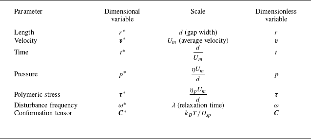
 Hsp
 kB
 T
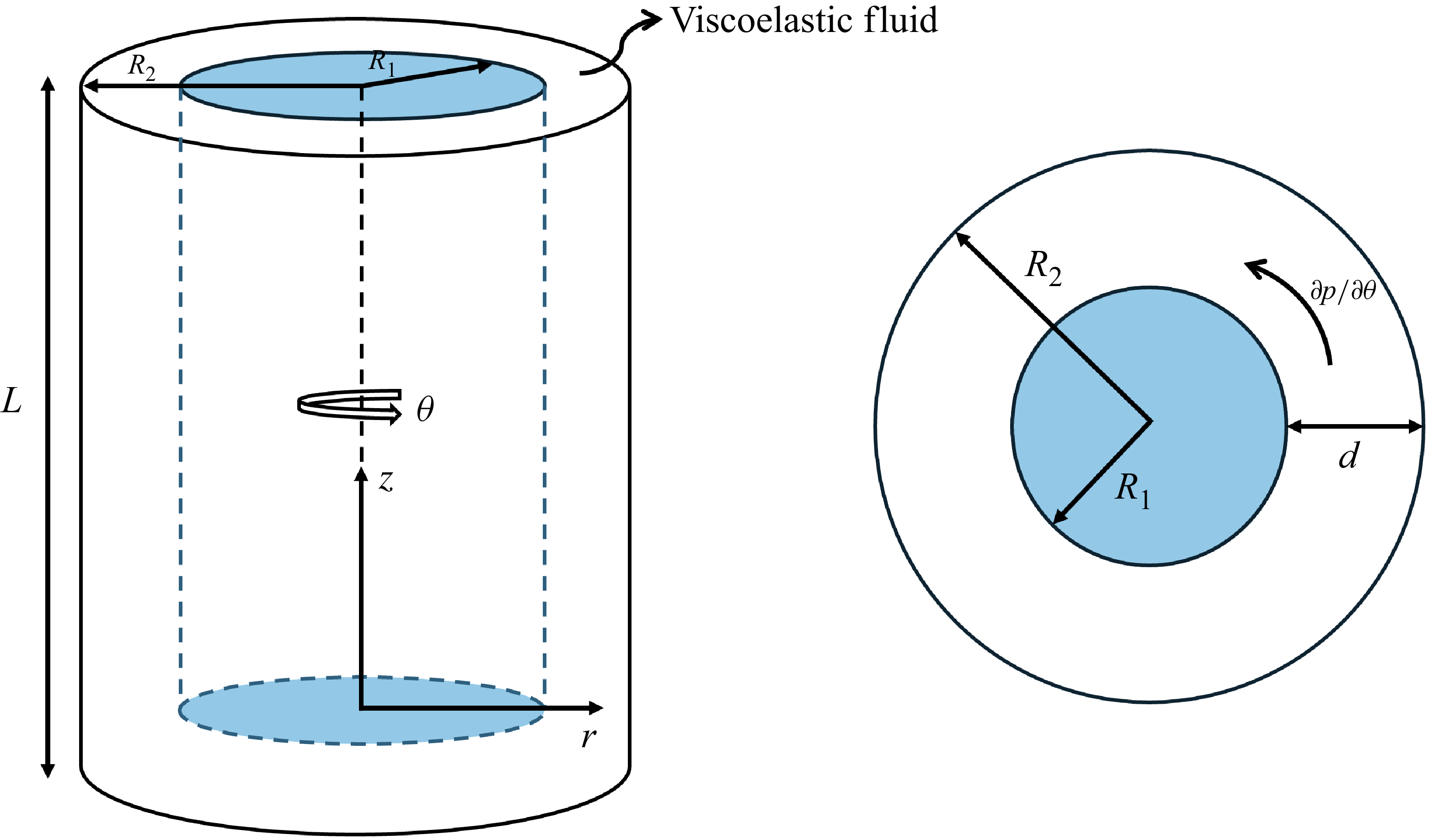

 β=0.98
 ϵ=0.1
 (Wi,L)
 Wi/L=10
 β=0.5
 ϵ=0.1
 Wi/L
 Wi/L
 Wi/L=10
 ϵ=0.1
 β
 Wi/L=10
 β=0.9
 ϵ

 (β=0)
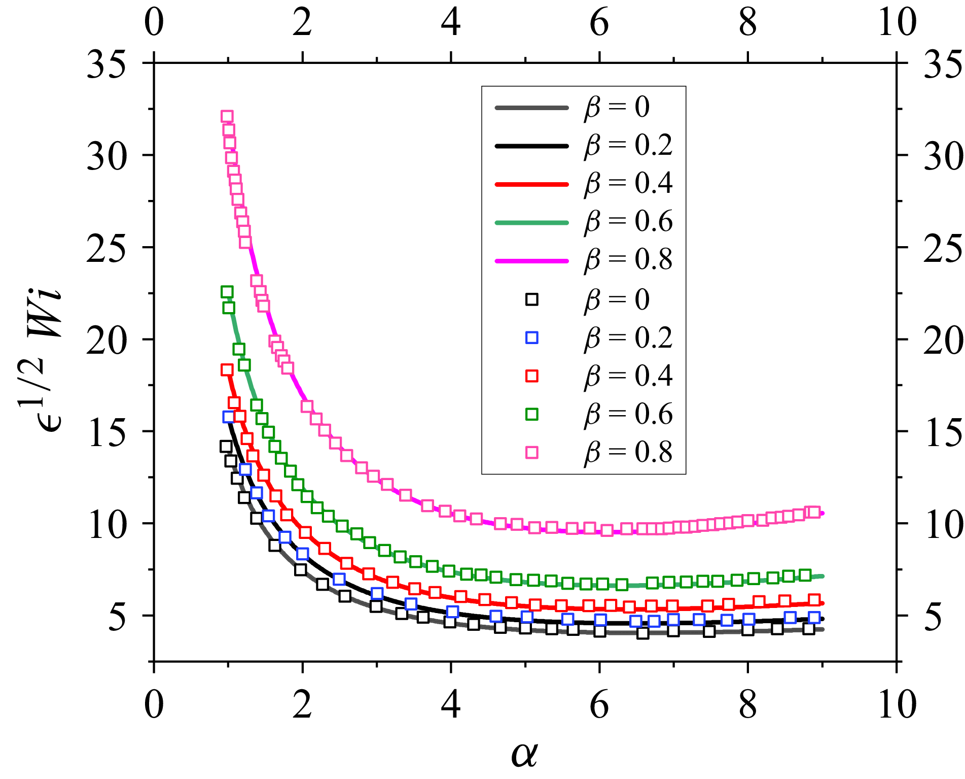
 Re=0
 n=0
 β

 α=7
 α=14
 Re=0
 n=0
 β=0.98
 ϵ=0.1
 Wi=25
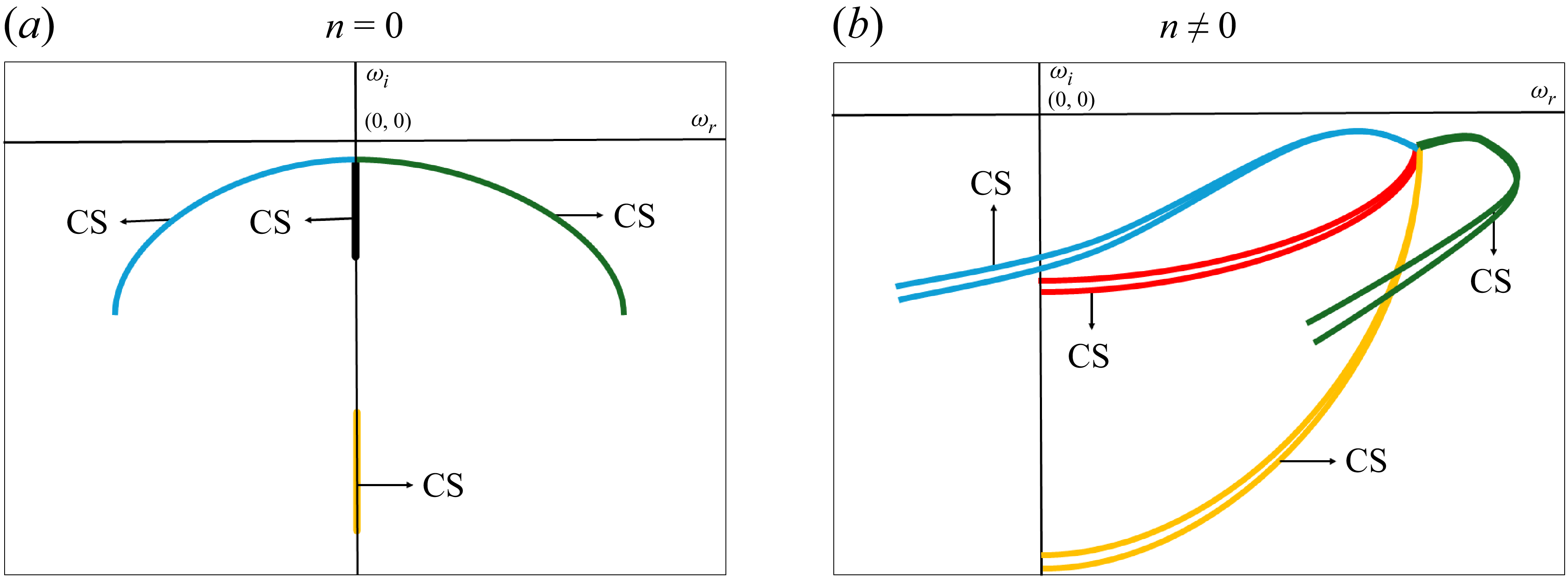
 Wi/L∼O(1)
 β→1
 n=0
 n≠0

 L
 n=0
 ϵ=0.1
 α=7
 β=0.98
 Wi=20
 Re=0
 L=104
 L=5000
 L=1000
 L=500
 L=398
 L=390
 L=150
 L=100

 n=1
 Wi=20
 L=200,Wi=400
 α=7
 β=0.98
 ϵ=0.1

 Re=0
 α=7
 β=0.98
 ϵ=0.1,n=1
 Wi
 Wi=20
 Wi=60
 Wi=200
 Wi=400
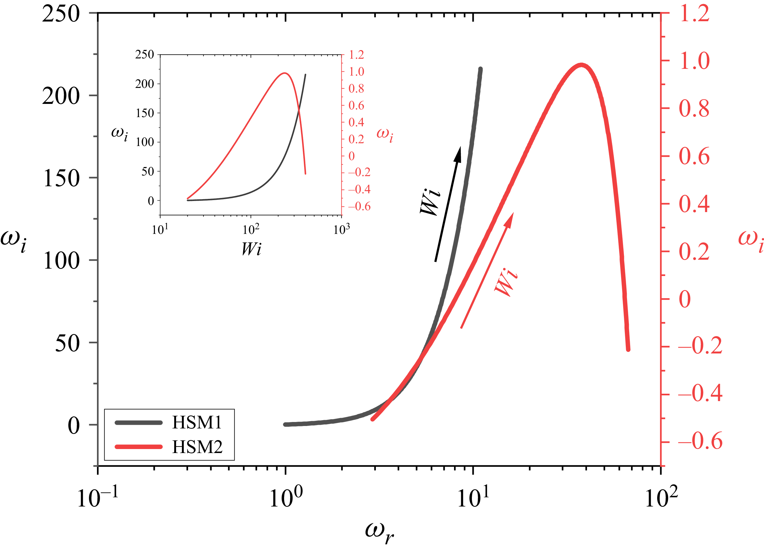
 Wi
 y
 Wi
 ωi
 Wi
 Re=0
 α=7
 β=0.98
 ϵ=0.1,n=1
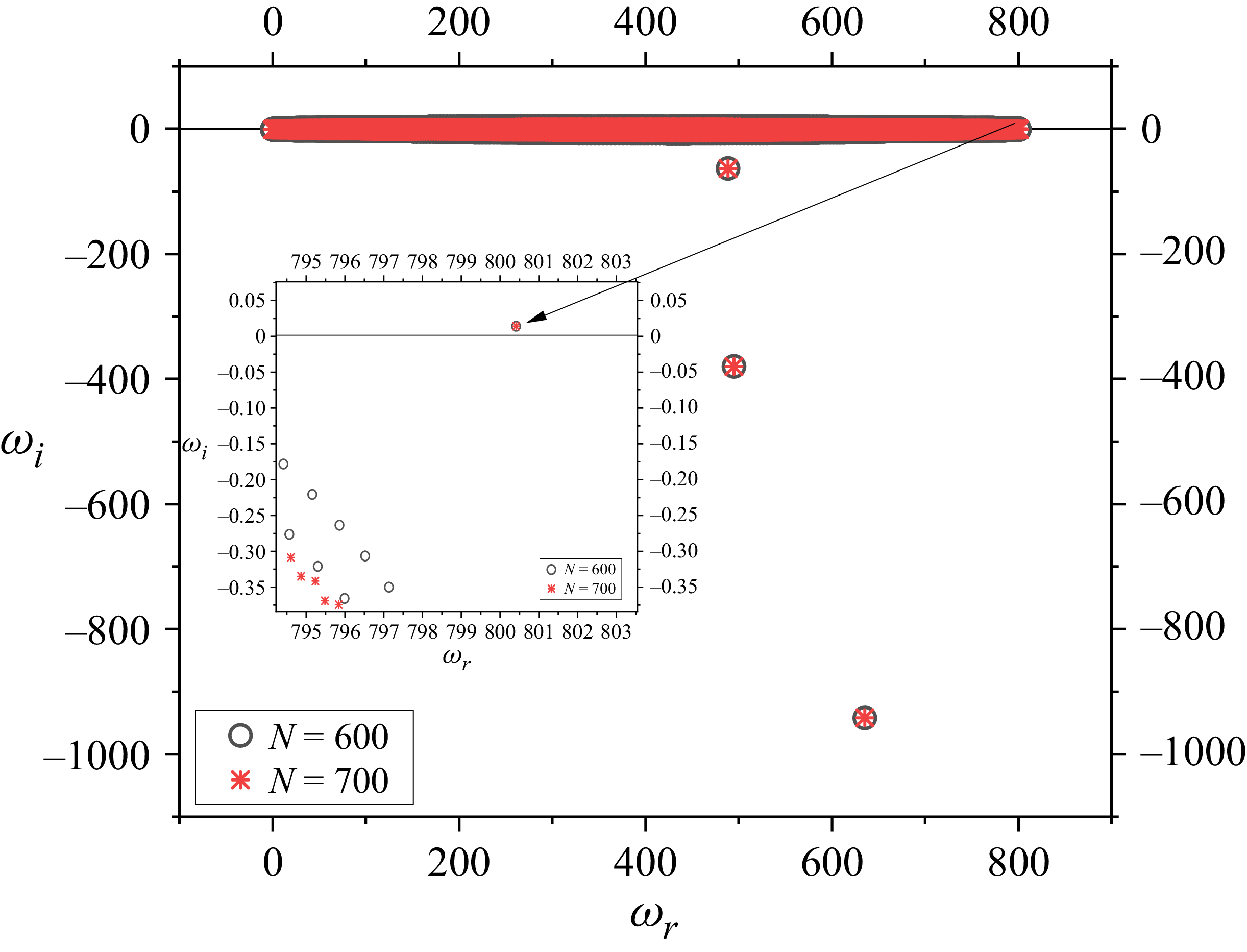
 n=16
 ϵ=0.1
 α=0
 β=0.994
 Wi=350
 N=600
 N=700
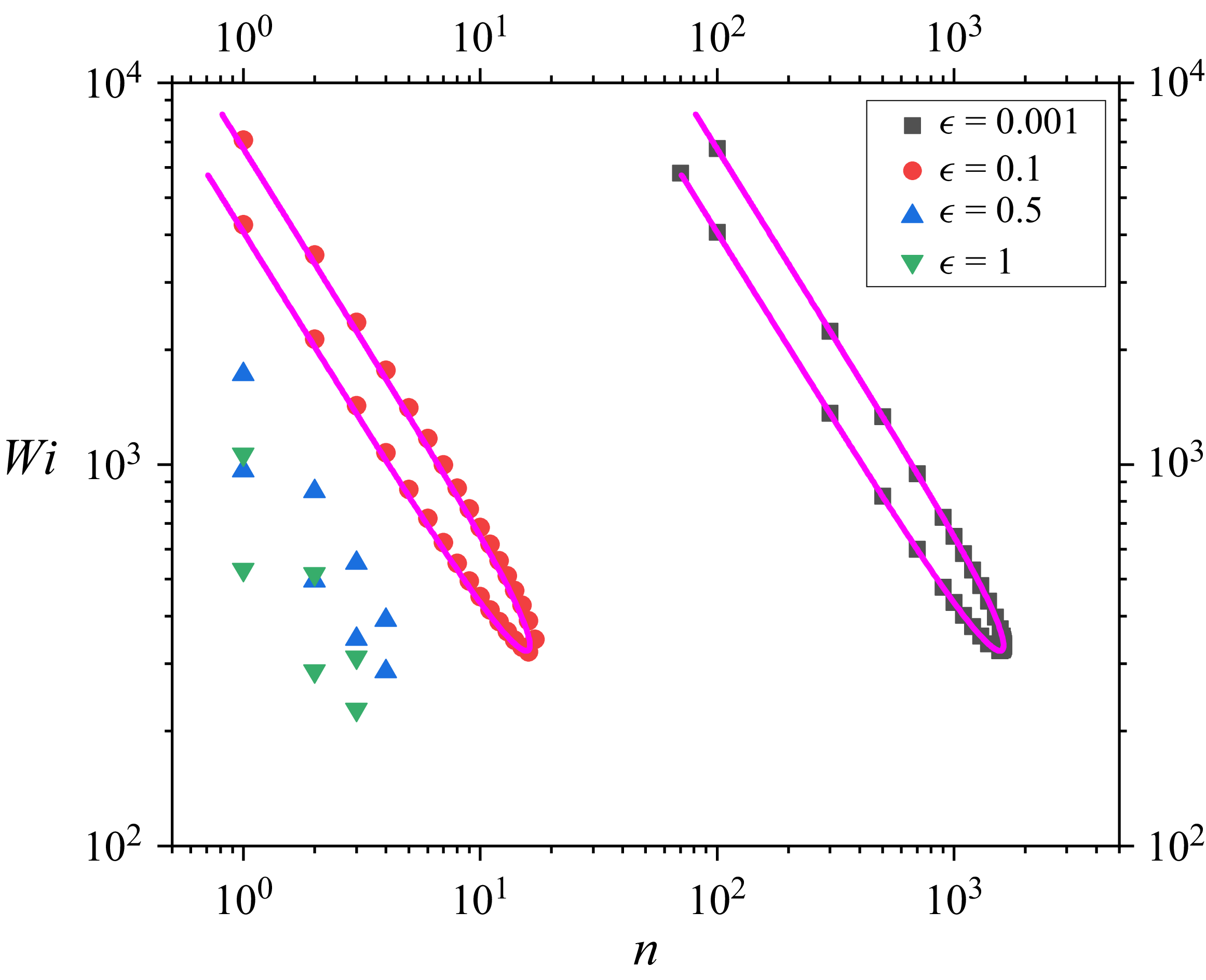
 Re=0
 α=0
 Wi
 n
 ϵ
 β=0.994
 ϵ=0.001
 0.1
 n∼ϵ−1
 ϵ=0.1

 y
 θ
 β=0.994
 α=0
 |v~θ|
 Wi=350
 ϵ=1
 Wi=230

 n=1
 ϵ=0.1
 β=0.98
 Wi=1500
 α=0
 α=0.5
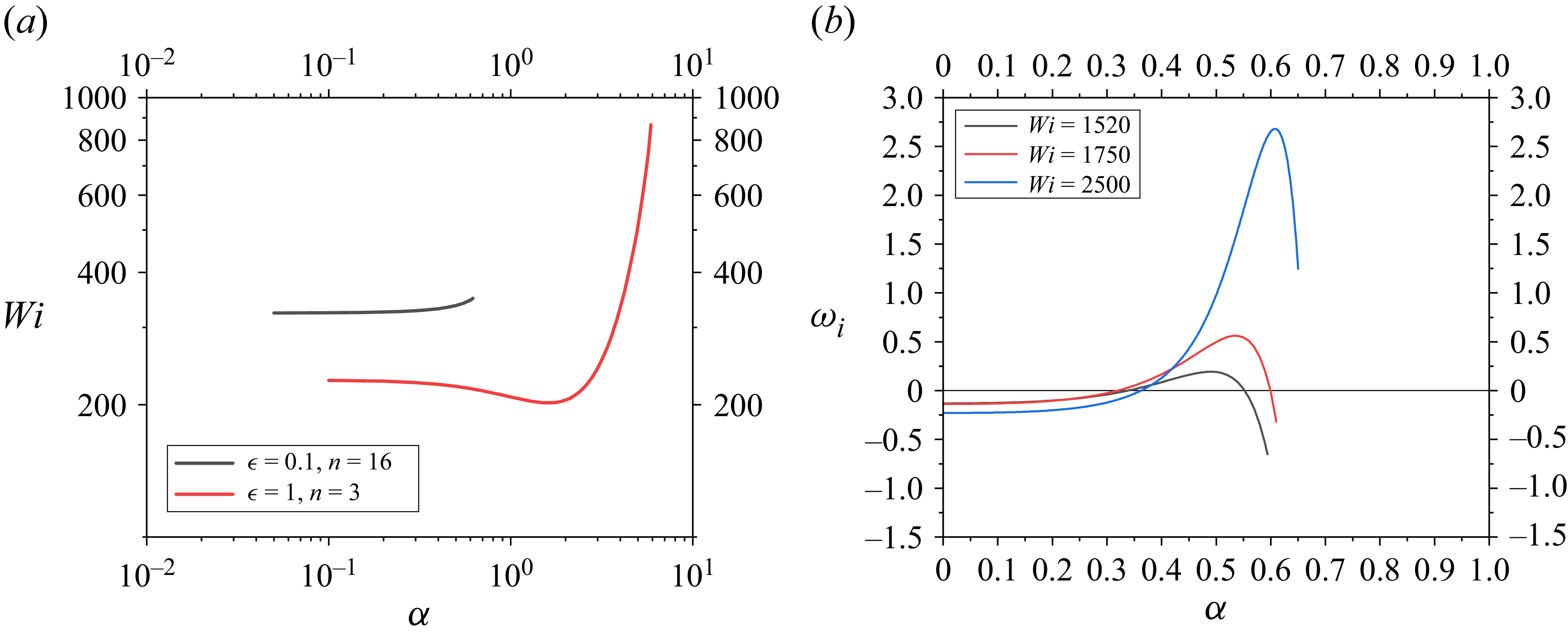
 Wi
 α
 ϵ
 n
 β=0.994
 ωi
 α
 α
 n=1
 ϵ=0.1
 β=0.98
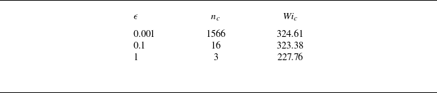
 (Wic)
 ϵ
 β=0.994
 Re=0
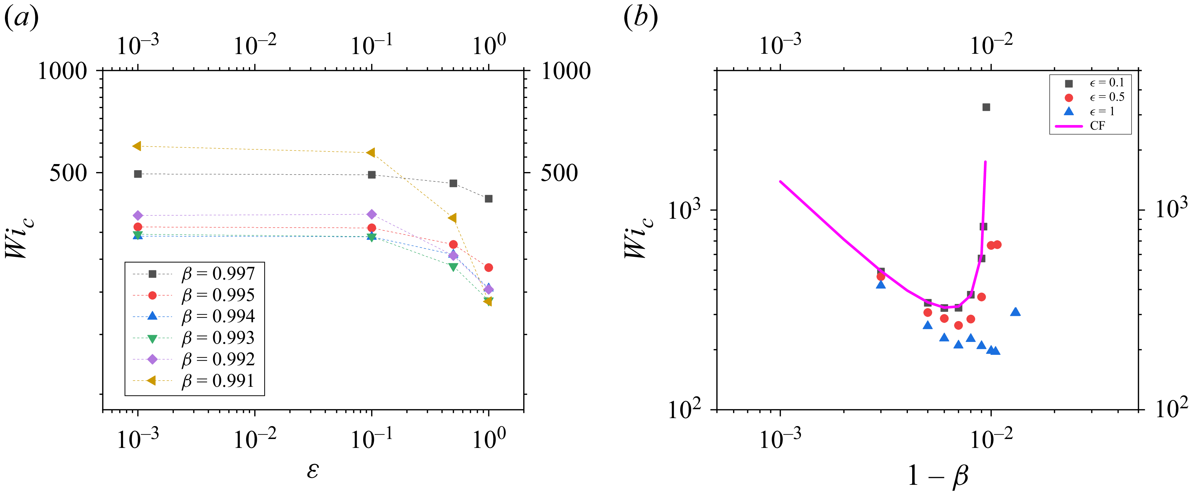
 Re=0
 α=0
 Wic
 ϵ
 β
 Wic
 (1−β)
 ϵ
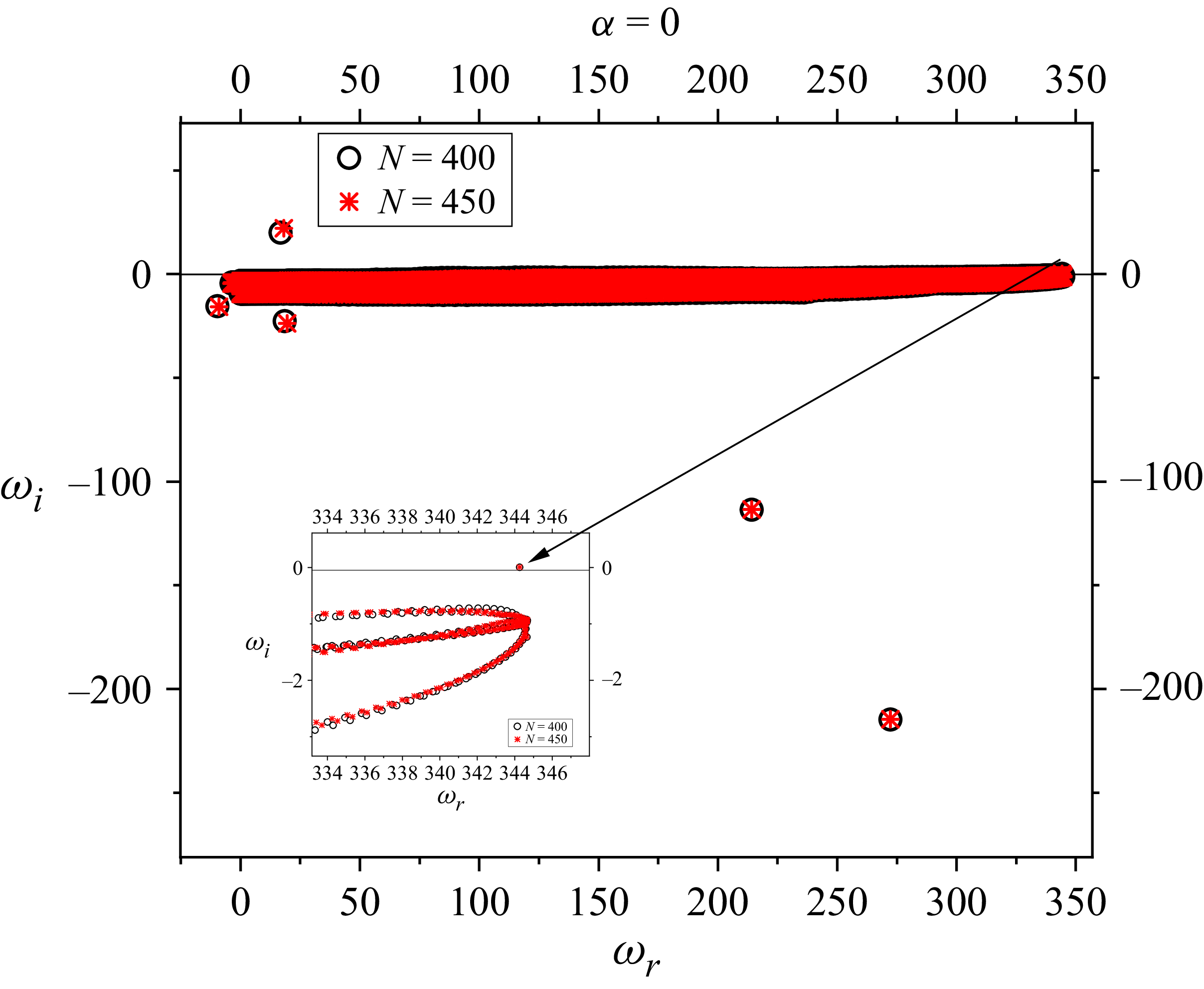
 n=40
 ϵ=0.1
 α=0
 β=0.98
 L=100
 Wi=60
 N=400
 N=450
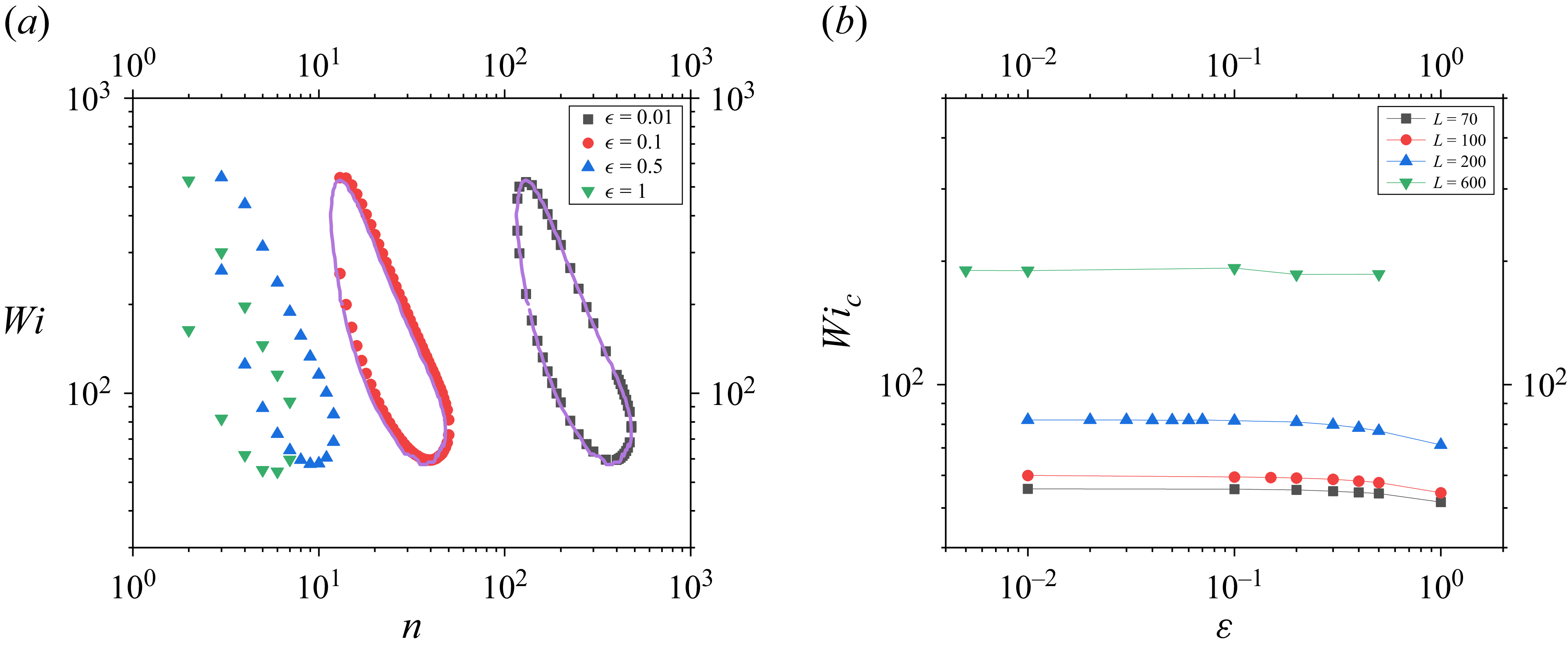
 ϵ
 L=100
 ϵ=0.01
 0.1
 Wic
 ϵ
 L
 Re=0
 α=0
 β=0.98
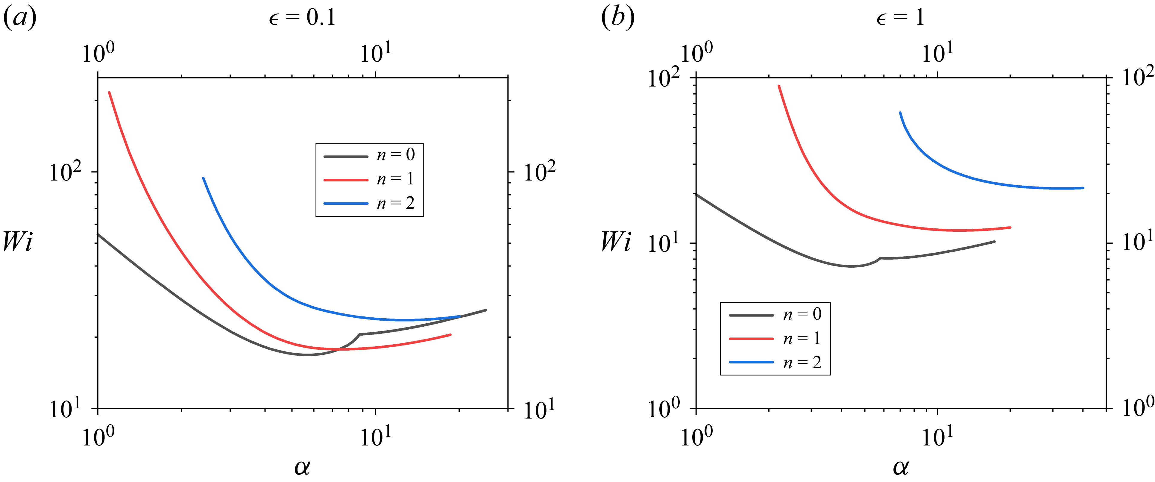
 ϵ
 ϵ=0.1
 ϵ=1
 Re=0
 β=0.98
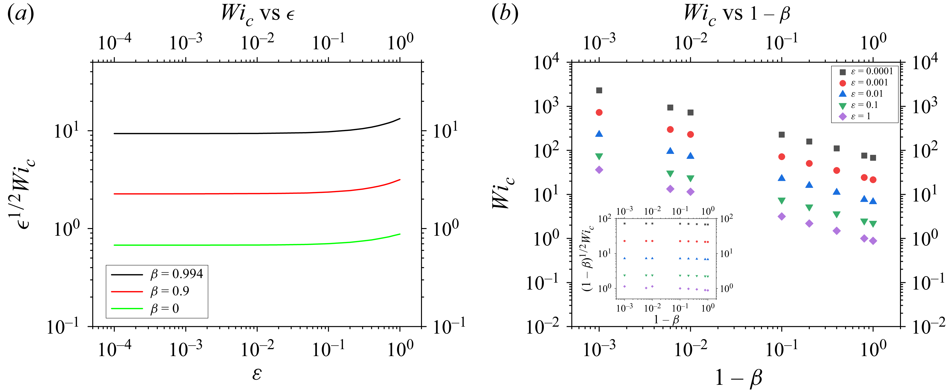
 (Wic)
 Re=0
 n=0
 ϵ1/2Wic
 ϵ
 β
 Wic
 1−β
 ϵ
 (1−β)1/2Wic
 β
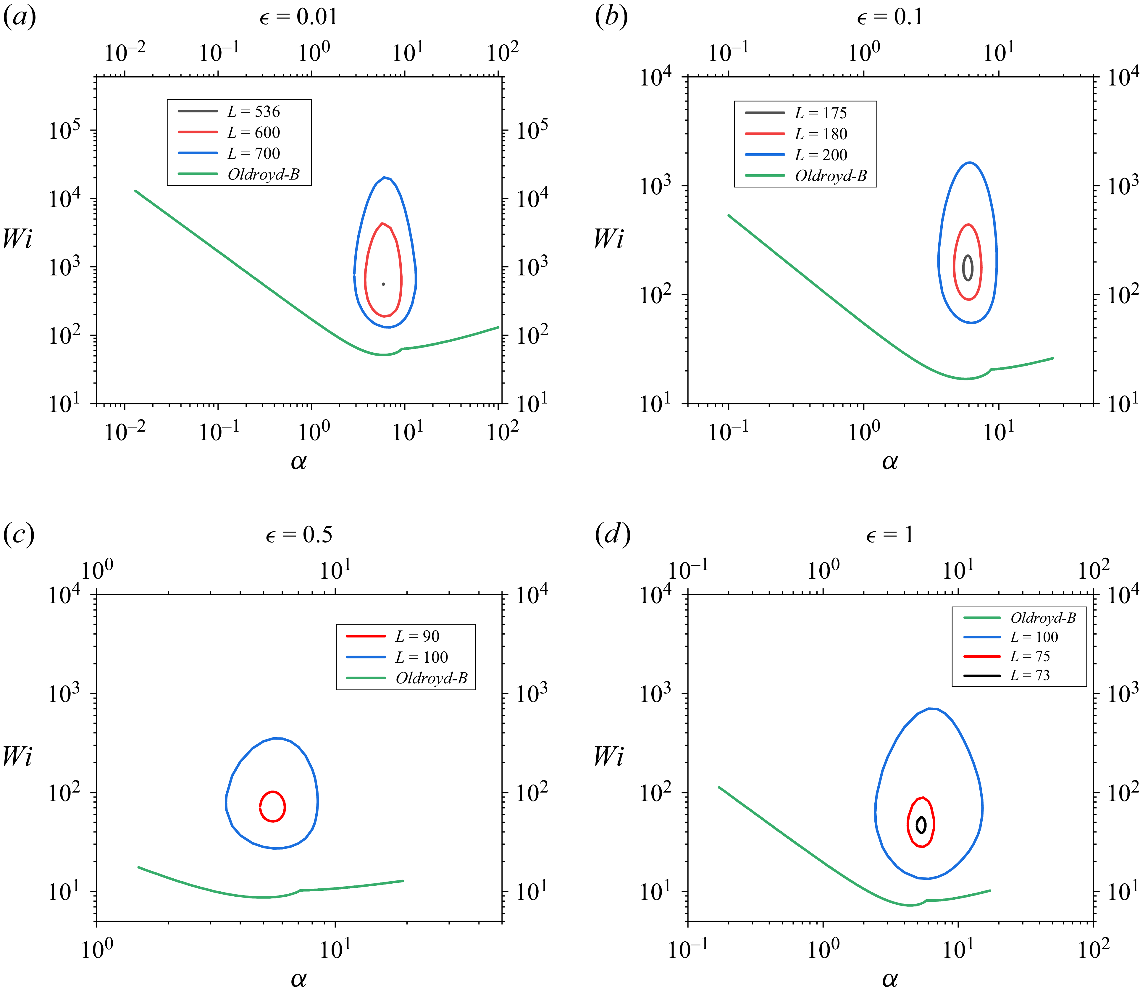
 Wi
 α
 Re=0
 β=0.98
 n=0
 ϵ=0.01
 ϵ=0.1
 ϵ=0.5
 ϵ=1
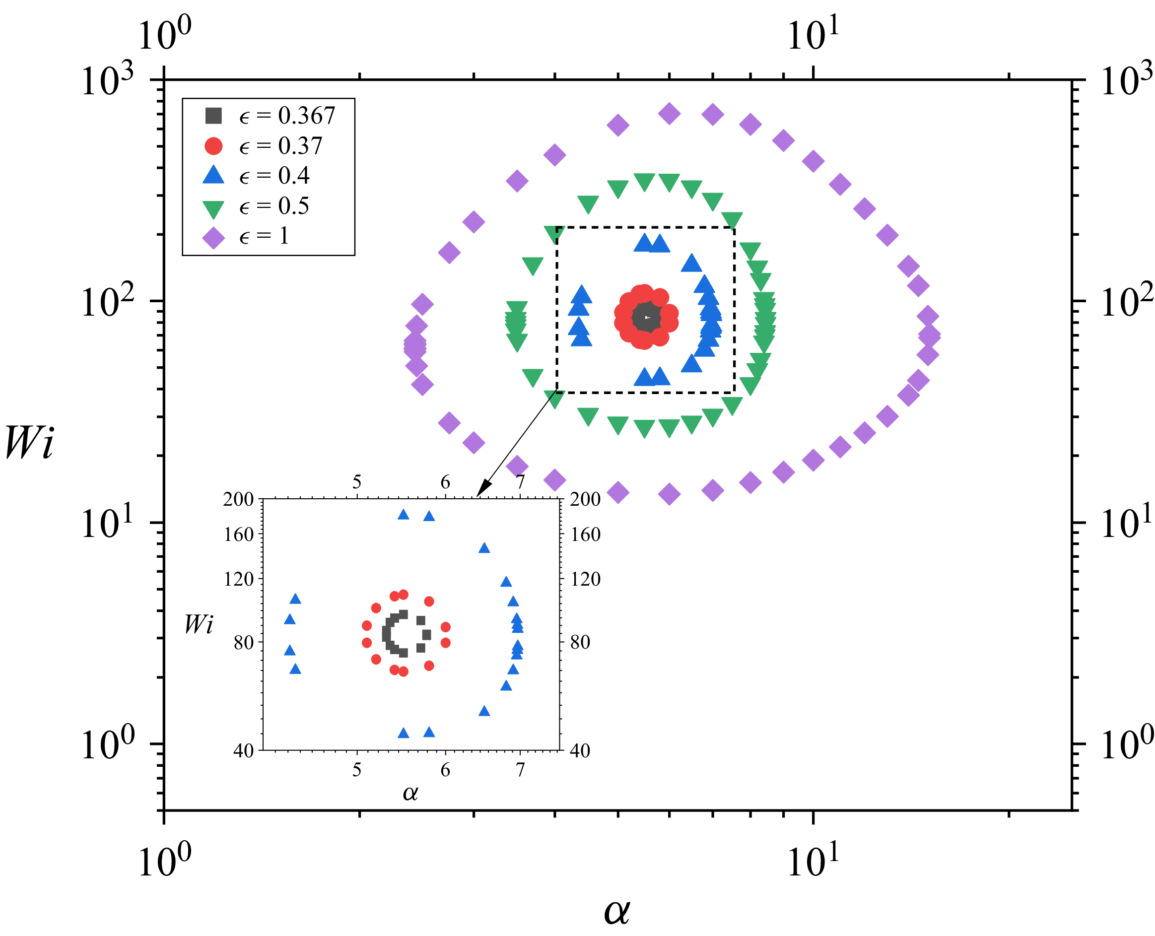
 ϵ
 ϵ≲0.36
 Re=0
 n=0
 β=0.98
 L
 40

 Re=0
 α=7
 β=0.98
 ϵ=0.1,n=1,Wi=400
 L
 L=106
 L=103
 L=100
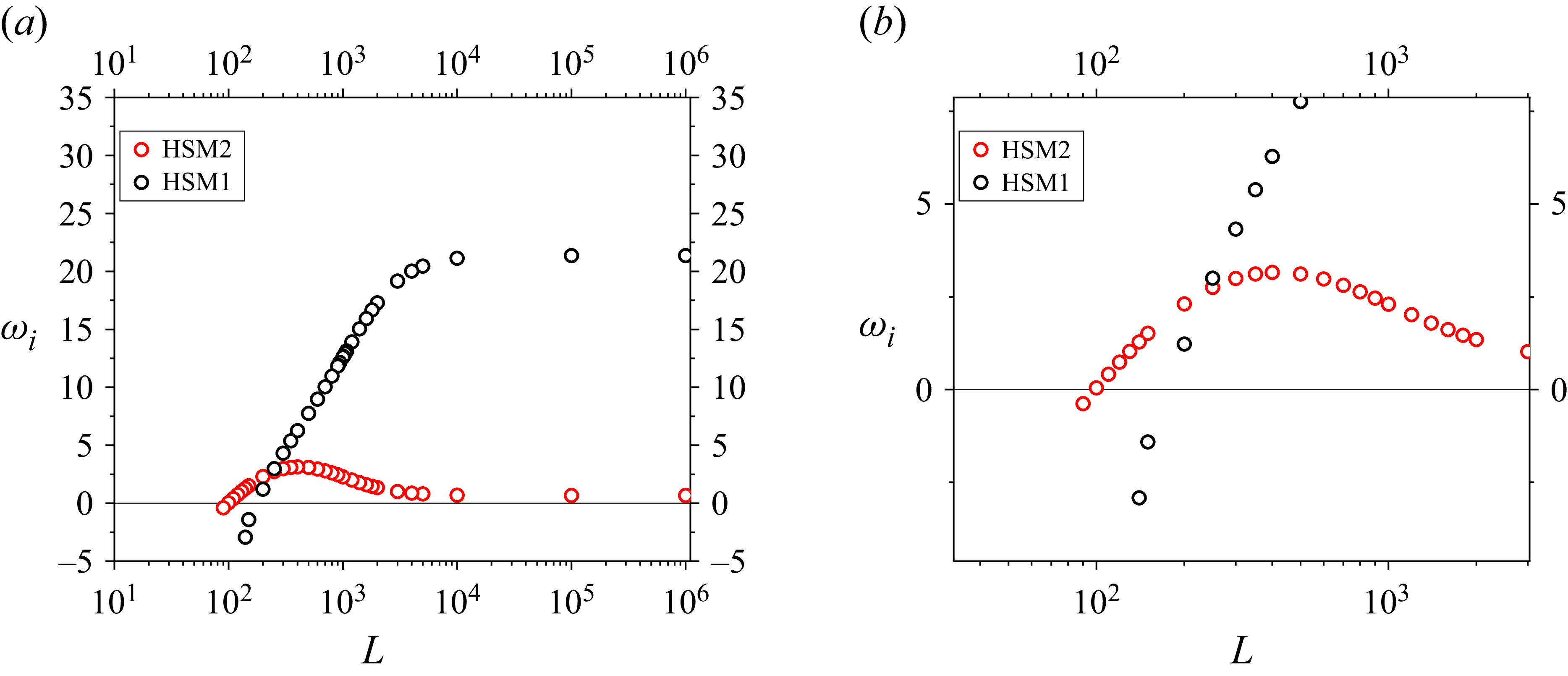
 ωi
 L
 ϵ=0.1
 α=7
 n=2
 Re=0
 Wi=130
 β=0.98
 10

 |v~θ|
 r−z
 β=0.98
 L=100
 Wi=400
 n=1
 α=7

 |v~θ|
 r−z
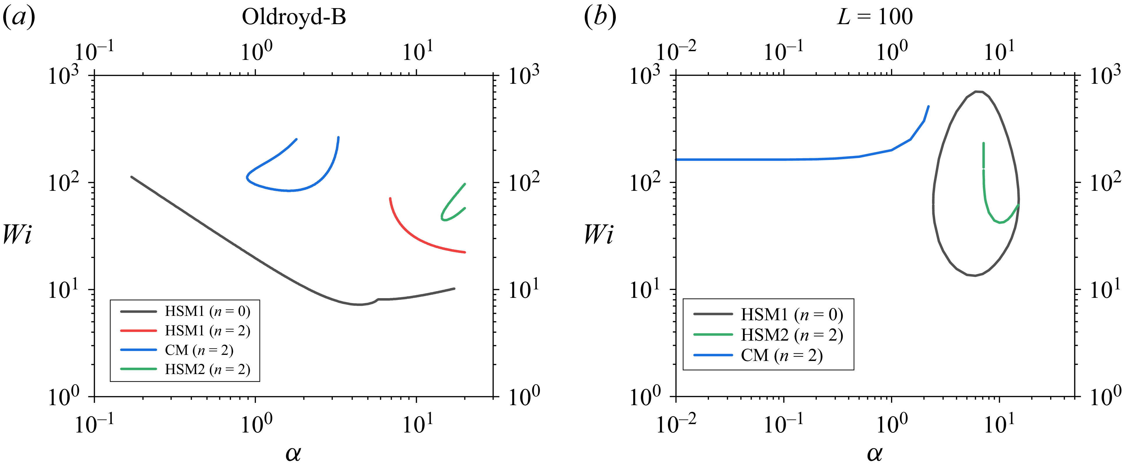
 L=100
 n=2
 Re=0
 ϵ=1
 β=0.98

 Re=0
 β=0.98
 L=100
 ϵ=0.1
 ϵ=0.2
 ϵ=0.5
 ϵ=1
 n≠0
 ϵ=0.1
 0.2
 ϵ=0.5
 1
 n=0
 ϵ=0.5
 1

 Wic
 ϵ
 L
 L
 nc
 ϵ
 nc
 αc
 Re=0
 β=0.98
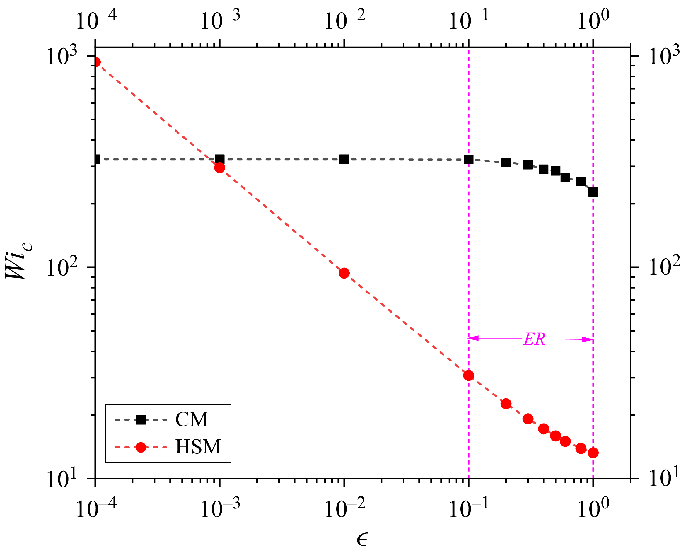
 ϵ<10−3
 ϵ>10−3
 Wic
 ϵ
 Re=0
 β=0.994
 ϵ
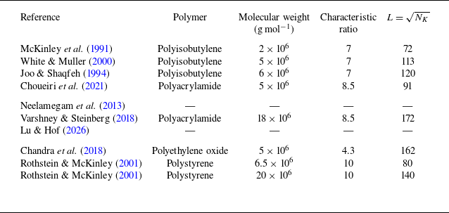
 L

 L
 ϵ
 Wic
 ϵ
 β=0.98
 Re=0
 ϵ
 L=600
 L=200
 L=100
 L=70

 n=0
 α
 Wi=20
 ϵ=0.1
 β=0.98
 α=2
 α=7
 α=8
 α=8.6
 α=8.7
 α=10

 n=0
 ϵ=0.1
 α=7
 β=0.98
 Wi
 Wi=1.6
 Wi=13
 Wi=13.5
 Wi=20

 n=0
 Wi
 ϵ=0.1
 α=7
 β=0.98
 L=100
 Wi=0.016
 Wi=0.16
 Wi=0.8
 Wi=1.6
 Wi=8
 Wi=20

 Re=0
 α=0.1
 β=0.98
 ϵ=0.1
 n=16
 Wi/L=2
 Wi
 L
 Wi
 L
 N=180
 200
 Wi=200
 L=100
 Wi=200
 L=100
 Wi=400
 L=200
 Wi=400
 L=200

 r
 θ
 ϵ=0.1
 β=0.98
 L=100
 Wi=60
 n=40
 α=0

 r
 θ
 ϵ=0.1
 β=0.98
 L=100
 Wi=400
 n=1
 α=7
 τ¯θθ

 r
 θ
 ϵ=0.1
 β=0.98
 L=100
 Wi=400
 n=1
 α=7
 τ¯θθ


