2. PROBLEM STATEMENT AND ANALYSIS

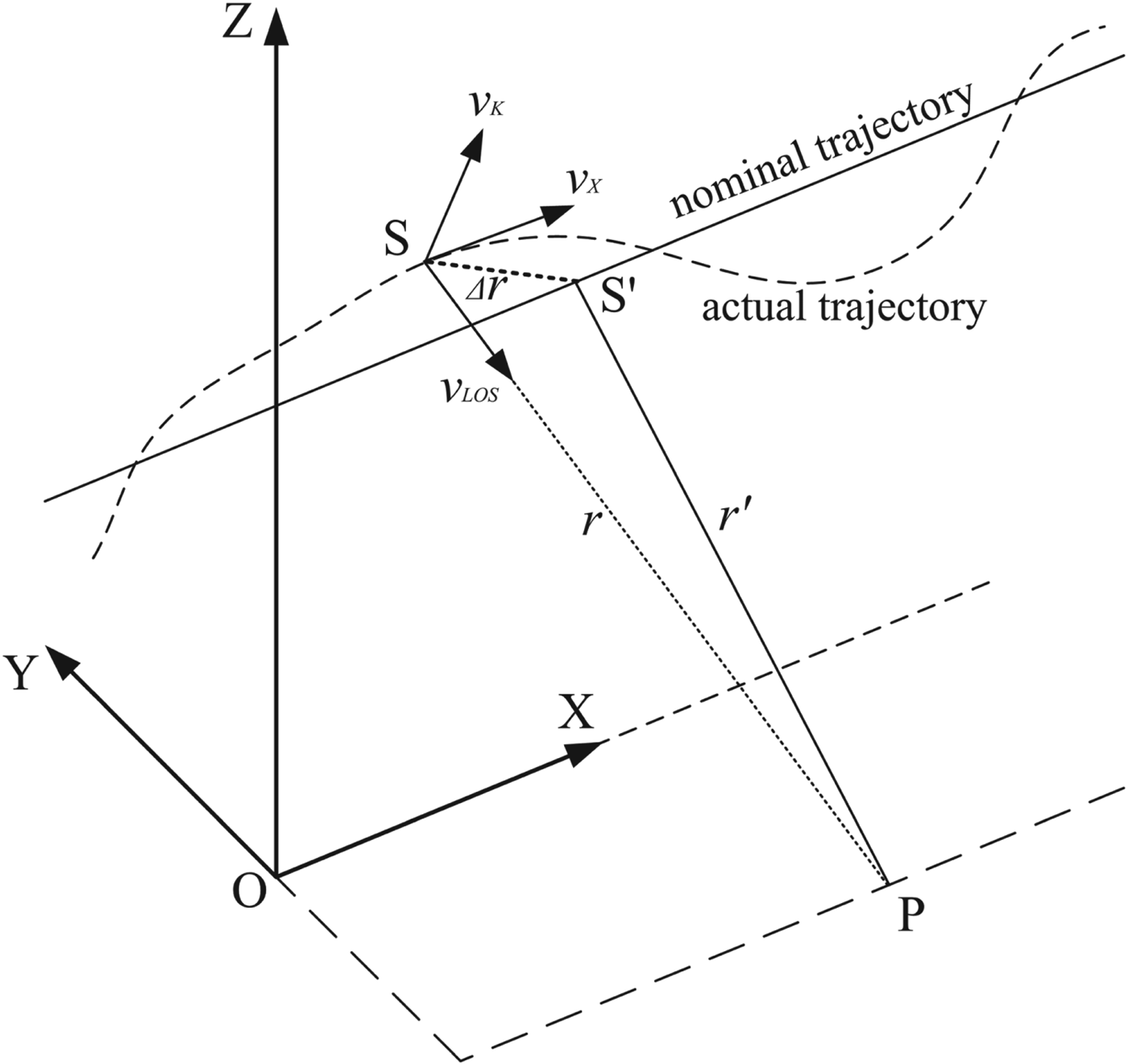
The deviation from the nominal trajectory is referred to as the motion error of SAR, and the geometry of SAR motion error is given in Figure 1, where the X-axis is the azimuth direction, the Y-axis is the range direction, the Z-axis is the vertical direction, S and S’ are the actual position and the corresponding nominal position of the SAR and P is the point target.

Figure 1.

Motion error geometry of SAR.

In a practical situation, the airborne platform cannot fly along the nominal trajectory (paralleling with the X-axis), so the velocities in the Y-axis and Z-axis directions are non-zero values which brings the motion error Δ r between the actual distance r (S to P) and the nominal distance r′ (S′ to P). To resolve the phase error in SAR caused by Δ r, the SAR instantaneous velocity at position S can be separated into three components (Zhang et al., Reference Zhang, Qiao and Xing2012): V _X (along the X-axis), V _LOS (along the SAR Line-Of-Sight (LOS) direction) and V _K (perpendicular to the plane of V _X and V _LOS) as shown in Figure 1.

V _K will not be taken into account in MOCO, since it has no effect on the Doppler echo signal of SAR. However, V _LOS with a non-zero value may cause the position error in the LOS direction, which is:

$$\Delta r_{LOS} (t)=\int_0^t {v_{LOS} (u)} du$$

The corresponding phase error of the SAR echo signal can be expressed as:

$$\Delta \Phi (t)=\displaystyle{4\pi \over \lambda} \Delta r_{LOS} (t) = \displaystyle{4\pi \over \lambda} \int_0^t {v_{LOS} (u)} du$$

where λ is the wavelength of the SAR. Then, the received echo signal can be modulated by the phase compensation exp( − jΔΦ(t)) to eliminate the phase errors.

Moreover, V _X is not constant in practice and this will directly cause the non-uniform sampling of the echo signal in the azimuth direction. The real-time adjustment of Pulse Repetition Frequency (PRF) is commonly used for solving this problem. Assuming the nominal velocity along the X-axis is V _X0 and the nominal PRF is P _rf0, the formula for calculating the real-time PRF value P _rf(t) is:

$$P_{rf} (t)=\displaystyle{V_X (t) \over V_{X0}} P_{rf0}$$

From Equation (3), the distance the SAR advances in the azimuth direction per pulse repetition interval is deduced as:

$$\Delta r_X = \displaystyle{V_X (t) \over P_{rf} (t)} = \displaystyle{V_{X0} \over P_{rf0}}$$

Since V _X0 and P _rf0 are both constant, the value of Δ r _X is also constant in time, thereby counteracting the effects of V _X changes on the echo signal.

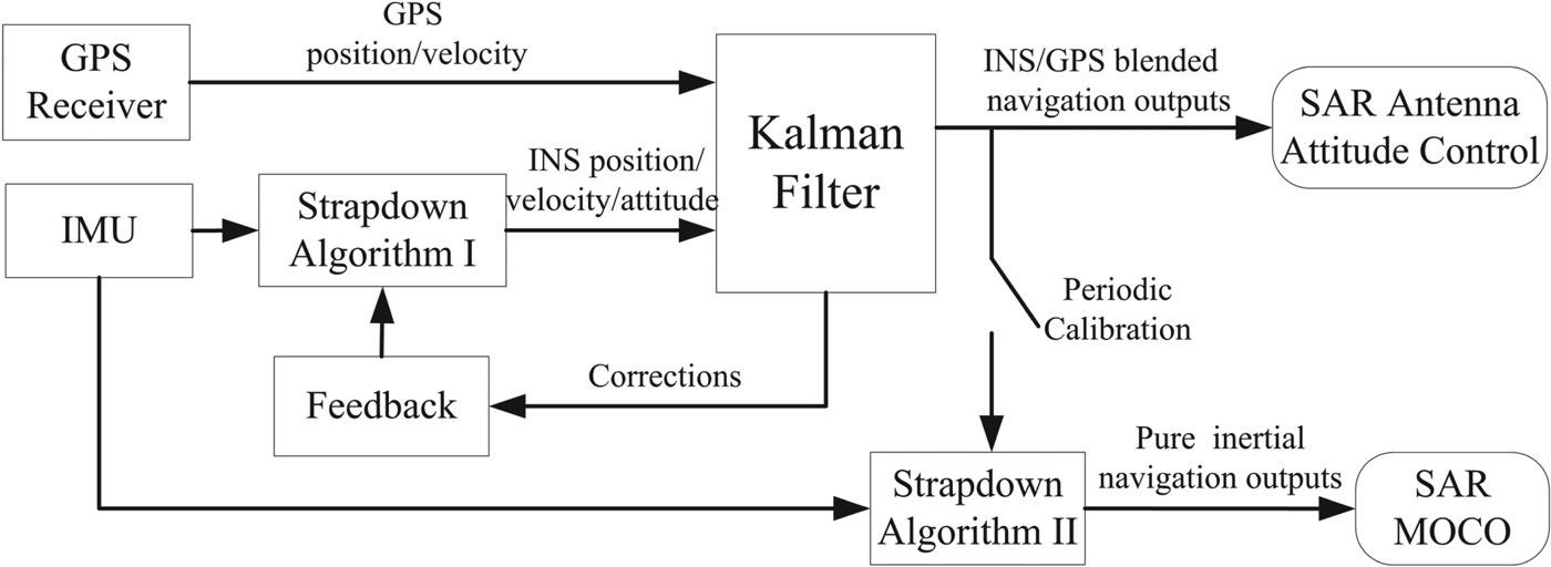
It can be shown very clearly from Equations (2) and (4) that proper MOCO processing of the collection of SAR measurements requires precise knowledge of the spatial location of the radar antenna with respect to the target scene for each and every pulse measurement. Furthermore, the image quality of the SAR depends on not only the accurate knowledge of position and velocity but also the smoothness of the relative change in position error and velocity error (Doerry, Reference Doerry2015). At present, the use of INS/GPS with a dual-strapdown algorithm (Guo et al., Reference Guo, Ding and Fang2004; Tan, Reference Tan2010) for motion compensation of SAR imaging has provided an important advance in picture quality and ability to accurately locate the radar antenna. Figure 2 shows the principle diagram of INS/GPS with a dual-strapdown algorithm. The outputs of Strapdown-Algorithm I and the GPS Receiver are input into the Kalman filter, which calculates corrections to the position, velocity and attitude data from Strapdown-Algorithm I. The corrections are applied to the outputs of Strapdown-Algorithm I with feedback compensation. Then the INS/GPS blended navigation outputs are used for two purposes: (1) Calibrate the outputs of Strapdown-Algorithm II at a constant periodicity (longer than the SAR imaging period to avoid large jumps in the position error and velocity error). (2) Control the attitude of the SAR antenna. Finally, Strapdown-Algorithm II provides pure inertial navigation outputs which are used for SAR MOCO.

Figure 2.

Block diagram of the INS/GPS with dual-strapdown algorithm.

Since the inertial navigation equations in Strapdown-Algorithm II integrate the error sources, such as accelerometer and gyro biases, the inertial navigation errors grow with time (Kaygısız and Sen, Reference Kaygısız and Sen2015; Li et al., Reference Li, Wang and Gao2016). The propagation of inertial navigation errors can be represented in mathematical form as a set of differential equations which are derived from the inertial navigation system equations (Han and Wang, Reference Han and Wang2011; Li and Fang, Reference Li and Fang2013; Li et al., Reference Li, Wang and Gao2016) by taking partial derivatives, which are shown in Equation (5):

$$\left\{\matrix{\delta \dot {L}=\displaystyle{\delta V_y \over R} \hfill \cr \delta \dot {\lambda} = \displaystyle{\delta V_x \over R}\sec L \hfill \cr \delta \dot{V}_x = 2\omega_{ie} \cdot \sin L\cdot \delta V_y -\varphi_y \cdot g+\nabla_x \hfill \cr \delta \dot{V}_y =-2\omega_{ie} \cdot \sin L\cdot \delta V_x +\varphi_x \cdot g+\nabla_y \hfill \cr \dot {\varphi}_x = -\displaystyle{\delta V_y \over R} +\varphi_y \cdot \omega_{ie} \cdot \sin L-\varphi_z \cdot \omega_{ie} \cdot \cos L+\varepsilon_x \hfill \cr \dot {\varphi }_y = \displaystyle{\delta V_x \over R}-\delta L\cdot \omega_{ie} \cdot \sin L-\varphi_x \cdot \omega_{ie} \cdot \sin L+\varepsilon_y \hfill \cr \dot {\varphi }_z =\displaystyle{\hbox{tg}\,L \over R} \delta V_x +\delta L\cdot \omega_{ie} \cdot \cos L+\varphi_x \cdot \omega_{ie} \cdot \cos L+\varepsilon_z}\right.$$

To be convenient for principal analysis, the Equations (5) are deduced on a stationary base without regard for the vertical channel, where δλ and δ L are the position errors, δ V _x and δ V _y are the velocity errors, φ_x, φ_y, and φ_z are the attitude errors, ∇_x and ∇_y are the accelerometer biases, ε_x, ε_y and ε_z are the gyro drift errors, ω_ie is the Earth rotational angular velocity, R is Earth's radius and g is gravitational acceleration.

The Laplace solution of Equation (5) is derived by Laplace transforms as follows:

$$\left\{\matrix{S\delta L(S) = \displaystyle{\delta V_y (S) \over R} + \delta L_0 (S) \hfill \cr S\delta \lambda (S)=\displaystyle{\sec L \over R}\delta V_x (S)+\delta \lambda_0 (S) \hfill \cr S\delta V_x (S)=2\omega_{ie} \cdot \sin L\cdot \delta V_y (S)-g\cdot \varphi_y (S)+\delta V_{x0} (S)+\nabla_x (S) \hfill \cr S\delta V_y (S)=-2\omega_{ie} \cdot \sin L\cdot \delta V_x (S)+g\cdot \varphi_x (S)+\delta V_{y0} (S)+\nabla_y (S) \hfill \cr S\varphi_x (S)=-\displaystyle{\delta V_y (S) \over R}+\omega_{ie} \cdot \sin L\cdot \varphi_y (S)-\omega_{ie} \cdot \cos L\cdot \varphi_z (S)+\varphi_{x0} (S)+\varepsilon_x (S) \hfill \cr S\varphi_y (S)=\displaystyle{\delta V_x (S) \over R} - \omega_{ie} \cdot \sin L\cdot \delta L(S)-\omega_{ie} \cdot \sin L\cdot \varphi_x (S)+\varphi_{y0} (S)+\varepsilon_y (S) \hfill \cr S\varphi_z (S)=\displaystyle{\hbox{tg}\,L \over R} \delta V_x (S)+\omega_{ie} \cdot \cos L\cdot \delta L(S)+\omega_{ie} \cdot \cos L\cdot \varphi_x (S)+\varphi_{z0} (S)+\varepsilon_z (S)}\right.$$

where S is the Laplacian operator, δ L ₀, δλ₀, δ V _x0, δ V _y0, φ_x0, φ_y0, φ_z0 are the initial alignment errors and L, R and g are constant on the stationary base.

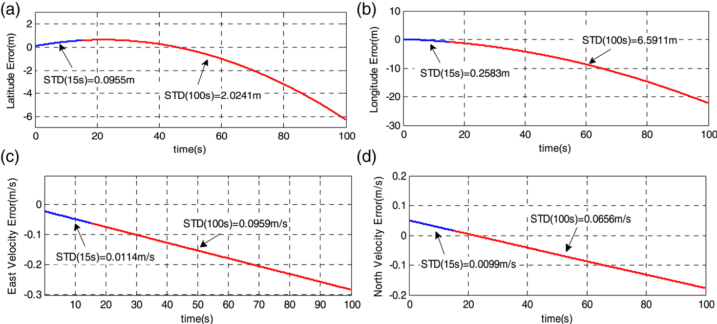
It is shown on the right side of Equation (6) that the errors in an inertial navigation system's position, velocity and attitude solution mainly arise from accelerometer biases, gyro drifts and initial alignment errors. Due to the inter-coupling of position errors, velocity errors, and attitude errors, full determination of inertial navigation error propagation is a complex problem and is invariably studied using a simulation method. Figure 3 shows simulation results of the position and velocity error propagation, which are the key factors in the MOCO processing. In Figure 3, the inertial navigation error accumulation in 15 s and 100 s are shown with blue lines and red lines.

Figure 3.

Simulation results of position and velocity error caused by gyro drift and accelerometer biases (gyro drift is 0·01^°/h, accelerometer biases are 50 ug, initial position error is 0·1 m, initial velocity error is 0·05 m/s, initial heading error is 3 arcminute, initial pitch and roll errors are both 1 arcminute). (a) Latitude error. (b) Longitude error. (c) East velocity error. (d) North velocity error.

When the SAR imaging period is short (for example, X-band, slant range 20 km, forward velocity 100 m/s, resolution 2 m, synthetic aperture time 5·8 s, MOCO duration time 15 s), the inertial navigation error accumulation of Strapdown-Algorithm II is not serious and the relative error noise is very low and smooth as shown by the blue lines in Figure 3. Thus, the outputs of Strapdown-Algorithm II are suitable for the SAR application with a short imaging period.

With the increasing demands of SAR applications, the synthetic aperture time is significantly prolonged (or there exist several continuous SAR imaging segments), and the imaging period might last for tens of seconds or even several minutes (Yang et al., Reference Yang, Xing and Zhang2012; Huang et al., Reference Huang, Liao and Yang2017). This means that the inertial errors of Strapdown-Algorithm II will constantly accumulate as shown by red lines in Figure 3, which is equivalent to introducing large absolute motion errors into the SAR MOCO. Therefore, the MOCO method based on INS/GPS with dual-strapdown algorithm cannot satisfy the requirements for SAR with long imaging periods.

3. DESIGN OF INS/GPS INTEGRATION ARCHITECTURE WITH DUAL-FILTER SMOOTHING CORRECTION

In order to restrain INS error divergence of Strapdown-Algorithm II in the previous section, GPS is the ideal choice as an external measurement to compensate for INS error (Chen and Fang, Reference Chen and Fang2014; Ye et al., Reference Ye, Liu, Li and Fang2018a). The optimum output provided by the integrated INS/GPS system is based on Kalman filter mechanisation. However, the use of a Kalman filter in a classical implementation would introduce discontinuities at the discrete updates of GPS data into the smooth inertial data. This paper aims to design a novel INS/GPS integration architecture for preventing INS error divergence and minimising the disturbing effects from discontinued Kalman updates. Furthermore, we take into consideration that SAR uses the navigation data in two principal manners: (1) Position and velocity data for motion compensation of the radar data (which emphasises the smooth character of motion compensation data); (2) Attitude data for SAR antenna pointing (which has no strict smooth requirement). Therefore, this paper proposes a MOCO method based on INS/GPS with dual-filter correction, which is suitable for SAR applications with long imaging periods.

First, we design a reduced-order open-loop Kalman filter (nine error-states) suitable for smoothing the position and velocity corrections. Open-loop correction architecture is chosen because estimated INS errors in the open-loop configuration are used to correct the inertial navigation outputs at each Kalman filtering iteration but are not fed back to the INS, and the good, smooth characteristics of the raw uncorrected inertial navigation outputs can be maintained. In order to reduce the computation load only position and velocity errors are estimated as the open-loop Kalman filter state. This is because motion compensation of the radar data just uses position and velocity information. A state propagation model has been developed for the open-loop Kalman filter. This model estimates position; resolves velocity errors referenced in the local navigation frame and addresses accelerometer biases. The state vector X comprises the following nine states:

$${\bi X}=\left[\matrix{\delta {\bi P}^n \hfill \cr \delta {\bi V}^n \hfill \cr {\bi \nabla}^n} \right], \quad \delta {\bi P}^n = \left[\matrix{\delta L \hfill \cr \delta \lambda \hfill \cr \delta h} \right], \quad \delta {\bi V}^{\,n} = \left[ \matrix{\delta V_E \hfill \cr \delta V_N \hfill \cr \delta V_U} \right],\quad {\bi \nabla}^n=\left[\matrix{\nabla_E \hfill \cr \nabla_N \hfill \cr \nabla_U} \right]$$

where the superscript n denotes the local navigation frame implementation, δPⁿ is the vector of position error expressed in terms of latitude error δ L, longitude error δλ, and height error δ h, δVⁿ is the vector of velocity error expressed in terms of east velocity error δ V _E, north velocity error δ V _N and up velocity error δ V _U, ${\bi \nabla} ^{n}$ is the vector of accelerometer biases.

The position and velocity error propagation are shown as follows:

$$\left\{\matrix{\delta \dot {L}=-\displaystyle{V_N \cdot \delta h \over (R_m +h)^2} + \displaystyle{\delta V_N \over R_m +h} \hfill \cr \delta \dot {\lambda} = \displaystyle{V_E \cdot \sec L\cdot \tan L\cdot \delta L \over R_n +h}-\displaystyle{V_E \cdot \sec L\cdot \delta h \over (R_n +h)^2} + \displaystyle{\sec L\cdot \delta V_E \over R_n +h} \hfill \cr \delta \dot {h}=\delta V_U \hfill \cr \delta \dot {{\bi V}}^{\,n}=-(2{\bi \omega}_{ie}^n +{\bi \omega}_{en}^n )\times \delta {\bi V}^{\,n}+(2\delta {\bi \omega}_{ie}^n +2{\bi \omega}_{en}^n )\times {\bi V}^{\,n}+{\bi \nabla}^n \hfill \cr \dot{\bi \nabla}^n=0 \hfill}\right.$$

where R _m, R _n are the meridian radius and the transverse radius, ${\bi \omega}_{ie}^{n}$ is the Earth rotation vector and ${\bi \omega}_{en}^{n}$ is the transport rate vector.

From Equation (8), the state vector X is described by the following dynamic and the observation models for Kalman filter state estimation are given as follows:

$$\left\{\matrix{\dot{{\bi X}}={\bi F}\cdot {\bi X}+{\bi G}\cdot {\bi w} \hfill \cr {\bi Z}={\bi H}\cdot {\bi X}+{\bi v} \hfill}\right.$$

where F and G denote the state transition matrix and the distribution matrix of the system noise, whose specific forms are derived from Equation (8). w denotes the system noise vector, whose components are considered as zero-mean random white noise. Z represents the observation vector, which is the difference of position and velocity between INS and GPS, calculated as follows:

$${\bi Z}=\left[\matrix{L_{INS} -L_{GPS} \cr {\lambda_{INS} -\lambda_{GPS} } \cr {h_{INS} -h_{GPS} } \cr {V_{E\_INS} -V_{E\_GPS}} \cr {V_{N\_INS} -V_{N\_GPS} } \cr {V_{U\_INS} -V_{U\_GPS}}} \right]$$

where H is the observation matrix, whose specific forms are defined as follows, and v is the observation noise vector, whose components are considered as zero-mean random white noise.

$$\left\{\matrix{{\bi H}=\left[\matrix{{\bi H}_1 &0_{6\times 3}} \right] \hfill \cr {\bi H}_1 =\left[\hbox{diag} \left(\matrix{R_m &R_n \cos L & 1 & 1 & 1 & 1} \right) \right]}\right.$$

Based on Equations (8)–(11), a nine error-states Kalman filter is constructed to obtain the estimations of position and velocity errors, $\delta \hat{L}(t)$, $\delta \hat {\lambda }(t)$, $\delta \hat{h}(t)$, $\delta \hat {V}_{E} (t)$, $\delta \hat {V}_{N} (t)$ and $\delta \hat {V}_{U} (t)$. Moreover, in order to diminish the discontinuity brought about by Kalman updates, we establish the smooth representation of position and velocity error estimations. Due to the requirement of low computational complexity and easy implementation, this paper uses a spline approximation algorithm for smoothing position and velocity error estimations. Taking the latitude error estimation $\delta \hat {L}(t)$ as an example, the spline smoothing algorithm is described as follows.

Suppose δ L(t) denotes the description of the real latitude error, and $\delta \tilde{L}(t)$ denotes the smoothed latitude error estimation. Let $e(t)=\delta L(t)-\delta \tilde{L}(t)$ denote the random error which is considered as zero-mean white noise with E[e(t)]=0, E[e(t _i)e(t _j)] = σ²δ(t _i − t _j) and σ is the variance of e(t).

Based on the cubic spline space, $\delta \tilde{L}(t)$ is taken as:

$$\delta \tilde{L}(t)=\sum_{i=1}^n {\delta \hat {L}(t_i )} \{{3(1-4\eta ) \Omega_3 (t - t_i ) - (1 - 6 \eta) \Omega _2^{(1/2)} (t-t_i )} \}$$

where n is the smoothing window value, η is the regulatory factor of different spline functions, Ω denotes the spline function and its expression form is given as:

$$\left\{\matrix{\Omega_2^{(1/2)} (t)=\Omega_2 \left(t+\displaystyle{1 \over 2} \right)+\Omega_2 \left(t-\displaystyle{1 \over 2} \right) \hfill \cr \Omega_k (t) = \displaystyle{\sum_{j=1}^{k+1} (-1)^j \left(\matrix{k+1 \cr j} \right) \left(t\,+\,\displaystyle{k+1 \over 2} - j\right)_+^k \over k!} \hfill \cr (t-t_0)_+^k = \left\{\matrix{(t-t_0)^k, \hfill & t\ge t_0 \hfill \cr 0, \hfill & t \lt t_0 \hfill}\right.\hfill}\right.$$

The calculation formula of η is as follows:

$$\eta = \displaystyle{2n\sigma ^2 \over 5(\delta \hat {L}^{2}(t_1 )+\delta \hat {L}^{2}(t_n ))+6\sum_{i=2}^{n-1} {\delta \hat {L}^{2}(t_i )} -8\sum_{i=0}^{n-1} {\delta \hat {L}(t_i )\delta \hat {L}(t_{i+1} )} +2\sum_{i=1}^{n-2} {\delta \hat {L}(t_i )\delta \hat {L}(t_{i+2} )}}$$

The obtained η value is substituted into Equation (12) to calculate $\delta \tilde{L}(t)$. Likewise, the smoothed estimations of other position and velocity errors $\delta \tilde{\lambda }(t)$, $\delta \tilde{h}(t)$, $\delta \tilde{V}_{E} (t)$, $\delta \tilde{V}_{N} (t)$ and $\delta \tilde{V}_{U} (t)$, can be calculated in the same way. Then, the smoothed navigation outputs, which are used for motion compensation of the radar data, L̃(t), $\tilde{\lambda }(t)$, h̃(t), $\tilde{V}_{E} (t)$, $\tilde{V}_{N} (t)$ and $\tilde{V}_{U} (t)$, are obtained from the raw inertial navigation solution, L _INS (t), λ_INS (t), h _INS (t), V _{E_INS} (t), V _{N_INS} (t) and V _{U_INS} (t), using:

$$\left\{\matrix{{\tilde{L}(t)=L_{{\rm INS}} (t)-\delta \tilde{L}(t)} \hfill \cr {\tilde{\lambda }(t)=\lambda_{{\rm INS}} (t)-\delta \tilde{\lambda }(t)} \hfill \cr {\tilde{h}(t)=h_{INS} (t)-\delta \tilde{h}(t)} \hfill \cr {\tilde{V}_E (t)=V_{E\_INS} (t)-\delta \tilde{V}_E (t)} \hfill \cr {\tilde{V}_N (t)=V_{N\_INS} (t)-\delta \tilde{V}_N (t)} \hfill \cr {\tilde{V}_U (t)=V_{U\_INS} (t)-\delta \tilde{V}_U (t)}}\right.$$

Second, since the INS errors estimated by the open-loop Kalman filter are not fed back every iteration to correct the INS itself, the error states will generally get larger as time progresses, which is likely to lead to large linearization errors of the open-loop Kalman filter in long-term navigation. Thus, the reduced-order open-loop Kalman filter presented above is designed to only work during the SAR imaging period. In order to provide the high long-term accuracy navigation outputs for SAR antenna pointing and the initial conditions (position, velocity and attitude) of INS/GPS integrated solution with the above reduced-order open-loop Kalman filter, we also construct a conventional Kalman filter (15 error-states) with closed-loop correction architecture. Since the position, velocity and attitude estimates are zeroed after each set of corrections is fed back, the closed-loop feedback process keeps the error states small and minimises the effect of neglecting higher order products of error states in the system model of Kalman filter. The system state equation and observation equation for the closed-loop Kalman filter state estimation are given as follows:

$$\left\{\matrix{{\dot {{\bi X}}}^{\prime} = {{\bi F}}^{\prime} \cdot {{\bi X}}^{\prime}+{{\bi G}}^{\prime}\cdot {{\bi w}}^{\prime} \hfill \cr {{\bi Z}}^{\prime} = {{\bi H}}^{\prime} \cdot {{\bi X}}^{\prime} + {{\bi v}}^{\prime} \hfill}\right.$$

where X^′ comprises 15 states, including three position errors, three velocity errors, three attitude errors, three accelerometer biases and three gyroscope drift errors. F^′ and G^′ denote the state transition matrix and the distribution matrix of the system noise, Z^′ represents the observation vector, H^′ is the observation matrix, whose specific forms are defined in Nassar (Reference Nassar2003). w^′ and v^′ denote the system noise vector and the observation noise vector, whose components are considered as zero-mean random white noise. The estimations of position error vector $\delta \hat {{\bi P}}(t)$, velocity error vector $\delta \hat {{\bi V}}(t)$ and attitude error matrix $\delta \hat {{\bi C}}_{b}^{n} (t)$ by the closed-loop Kalman filter are fed back to the INS on each Kalman filter iteration. The Kalman filter's position, velocity, and attitude estimations are zeroed after each set of corrections is fed back. In closed-loop configuration, the feedback corrections are applied using:

$$\left\{\matrix{{\hat{{\bi P}}(t+)=\hat {{\bi P}}(t-)-\delta \hat {{\bi P}}(t)} \hfill \cr {\hat {{\bi V}}(t+)=\hat {{\bi V}}(t-)-\delta \hat {{\bi V}}(t)} \hfill \cr {\hat {{\bi C}}_b^n (t+)=\delta \hat {{\bi C}}_b^{n {\rm T}}(t)\hat {{\bi C}}_b^n (t-)}}\right.$$

where the suffixes (−) and (+) denote before and after the correction.

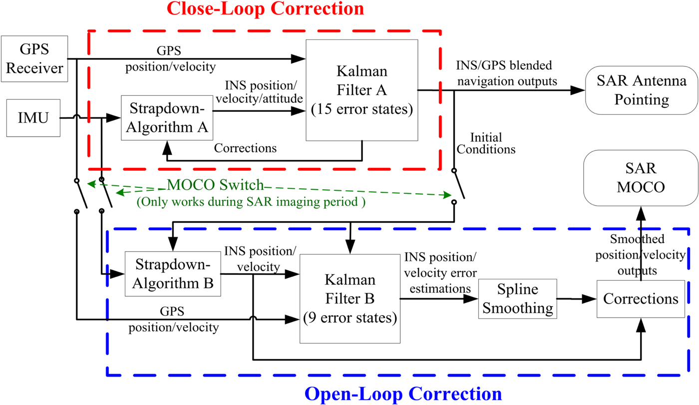
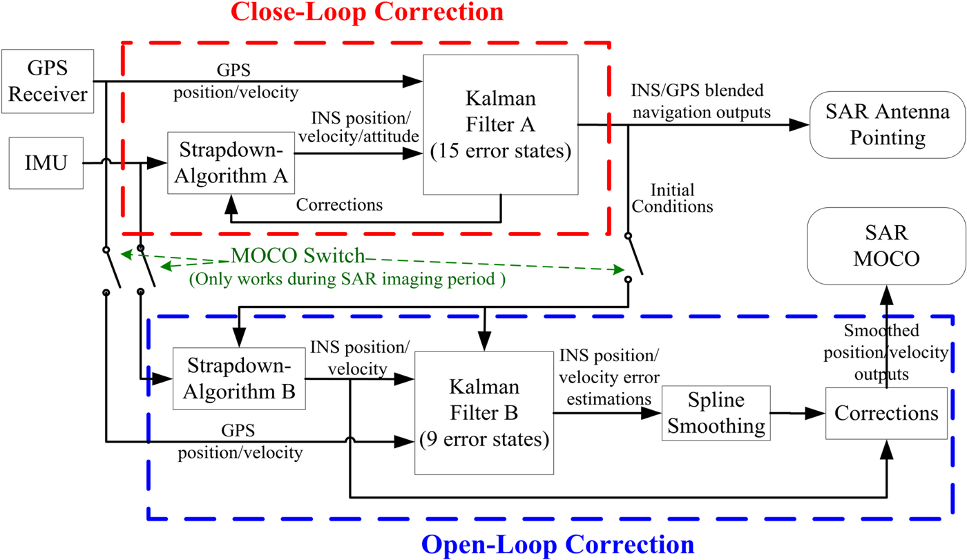
The principle block diagram of the proposed MOCO method based on INS/GPS with dual-filter correction is shown in Figure 4. When SAR does not run, MOCO switches are turned off, meaning that Strapdown-Algorithm B and Kalman filter B are both in a non-working state. In this case, the whole system works in the conventional INS/GPS integrated navigation mode with close-loop correction, and SAR antenna pointing is based on the obtained, highly accurate, long-term navigation outputs. As SAR imaging begins to operate, MOCO switches are simultaneously closed. Strapdown-Algorithm B executes the inertial navigation solution with the gyro and accelerometer outputs, while the initial conditions (position, velocity and attitude) are obtained from the outputs of Kalman filter A at the preceding moment. The INS position and velocity errors are estimated by Kalman filter B using GPS outputs as the observation information. Then, the INS position and velocity error estimations are processed by the smoothing module, and are applied to calibrate the outputs of Strapdown-Algorithm B with open-loop correction. Finally, the smoothed position and velocity outputs are provided to MOCO unit for forming the SAR image.

Figure 4.

Block diagram of the INS/GPS with dual-filter correction.

4. EXPERIMENT AND RESULT ANALYSIS

Since it is difficult to find a continuous, high-bandwidth comparison reference for INS/GPS in a dynamic environment, we use a simulation method to prove the precision of the proposed method in this paper. Then, in order to verify the effectiveness of the proposed method in a real SAR application, a flight experiment was carried out in an area near Yanliang, China, and the flight data was collected by Beihang University, Beijing, China.

4.1. Simulation Experiment

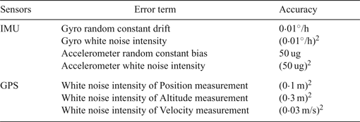
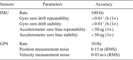
The device accuracy of INS/GPS is set as shown in Table 1.

Table 1.

Device accuracy of INS/GPS.

The outputs of Gyro, Accelerometer, and GPS are derived by a trajectory generator, with the sensor errors of Table 1 added. The simulation experiment was designed based on the requirements of SAR imaging. According to the motion mode of SAR imaging, a U-shaped trajectory is commonly adopted. In this paper, the flight trajectory is designed as follows:

1. (1) At initial time, latitude was 47^°N, longitude was 115^°E, altitude was 3,000 m, attitude was maintained as locally level, azimuth was 045^° and velocity was 100 m/s.

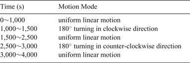
2. (2) The velocity and altitude were kept constant during the flight process, and the roll angular variations were considered at the manoeuvring turn. The flight process setting is described in detail in Table 2.

Table 2.

Flight process setting.

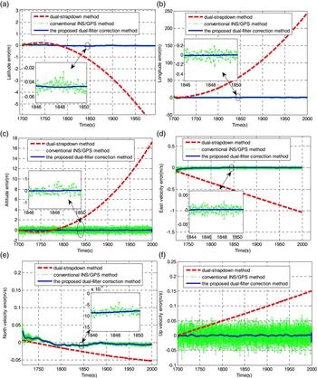
The 300 seconds data of 1,700 s~ 2,000 s time interval (the hypothetical SAR imaging period) is regarded as the verification range. We processed the INS/GPS integration by three different methods: the dual-strapdown method, the conventional INS/GPS method and the proposed dual-filter correction method. The accuracy results of motion compensation data (position and velocity) are compared in the same verification range.

Figure 5 shows the position and velocity error curves of the three methods mentioned above. The position and velocity errors of the dual-strapdown method greatly increase during the 300 s verification range, since there is no GPS information for updating the INS position and velocity components. However, the position and velocity error curves of the dual-strapdown method have favourable smoothness owing to the dead reckoning of pure inertial navigation. Compared with the dual-strapdown method, the conventional INS/GPS method has a much better performance in that its position and velocity errors maintain a good convergent trend. However, discontinuities are obviously introduced into the navigation outputs at each discrete update of GPS data, so the position and velocity error curves of the conventional INS/GPS method exhibit a marked serration. Ultimately, both methods can result in the inability to satisfy the requirement of SAR with long imaging periods.

Figure 5.

Position and velocity errors. (a) Latitude error. (b) Longitude error. (c) Altitude error. (d) East velocity error. (e) North velocity error. (f) Up velocity error.

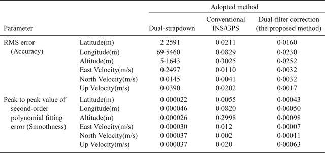
The proposed dual-filtering correction method has excellent comprehensive properties, combining the advantages of the other two methods, which can obtain high accuracy position and velocity motion parameters as well as ensuring smoothness. Table 3 shows the error statistics of the three methods for the 300 s verification range. The error accuracy is generated by calculating its Root-Mean-Squared (RMS) error, and the smoothness is obtained by calculating the peak to peak value of second-order polynomial fitting error (Cheng et al., Reference Cheng, Xiong and He2009).

Table 3.

Position/velocity accuracy and smoothness of different methods.

As seen in Table 3, although the smoothness of the dual-strapdown method is the best, its accuracy is the poorest of the three methods. The conventional INS/GPS method achieves better performance in accuracy than the dual-strapdown method but is unsatisfactory in smoothness. In the proposed dual-filter correction method, the position and velocity are more accurate than 0·0252 m and 0·0038 m/s, which outperforms those of the other two methods. The smoothness of position and velocity achieve 0·00098 m and 0·00063 m/s, several orders of magnitude higher than those of the conventional INS/GPS method and just slightly weaker than the dual-strapdown method. Clearly, the proposed dual-filter correction method provides outstanding integrated performance on both accuracy and smoothness among the three methods, which is suitable for SAR MOCO with long imaging periods.

4.2. Flight experiment with SAR

The proposed method was applied for a high-precision Laser INS/GPS integrated system (TX-L20-A2) developed by Beihang University, comprising of a Ring-Laser Gyro (RLG)-based IMU, a Novatel DL-V3 GPS receiver and a navigation computer. The experimental strip-mode SAR system operated in X-band (9·5 GHz) with a bandwidth of 180 MHz. The slant range of the scene centre was 15 km. The INS/GPS integrated system and the SAR system were installed on an Y7-Airplane, and the IMU was mounted on the rigid platform of the SAR antenna with a servomechanism to control the beam direction. The specifications of TX-L20-A2 INS/GPS are listed in Table 4.

Table 4.

Specifications of TX-L20-A2 INS/GPS.

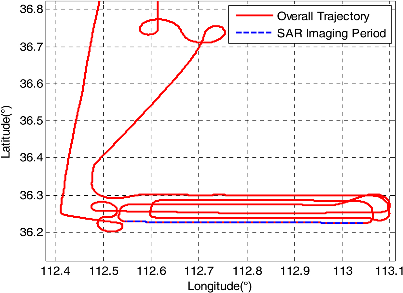
The flight experiment lasted for five hours, and the flight trajectory is shown in Figure 6. In the flight experiment region, the Y7-Airplane flew at a height of about 3,000 m, at a speed of 75–80 m/s. We select the data of several continuous SAR imaging segments to evaluate the effectiveness of the proposed dual-filter correction method, and the SAR imaging period lasted 268 seconds which is indicated by a blue dashed line in Figure 6.

Figure 6.

Trajectory of flight experiment.

The raw SAR data with a resolution of 1 m×1 m was collected by a strip-mode SAR system. The IMU and GPS data collected by TX-L20-A2 INS/GPS integrated system were processed by three different methods (the dual-strapdown method, the conventional INS/GPS method and the proposed dual-filter correction method). The three processing results were respectively used to complete the motion compensation in the SAR raw data.

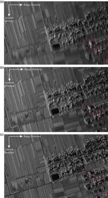
The images in Figure 7 were generated by motion compensation data from the three different INS/GPS methods. The vertical direction is azimuth, and the horizontal direction is range. The image achieved by the dual-strapdown method shown in Figure 7(a) is seriously blurred and distorted in geometry. This is because the pure inertial navigation results could not compensate for the low frequency motion errors due to the inertial errors accumulation during long imaging period.

Figure 7.

SAR images with different MOCO methods. (a) Dual-strapdown method. (b) Conventional INS/GPS method. (c) The proposed dual-filter correction method.

The conventional INS/GPS method achieves good performance in compensating the low frequency motion errors. The imaging result obtained via this method is shown in Figure 7(b) which is better when compared with Figure 7(a). Nonetheless, the discontinuities caused by the discrete updates of GPS data bring severe high frequency motion errors into the MOCO process, so the objects, highlighted in Figure 7(b) by red circles, appear distorted in the azimuth direction.

Owing to the effective treatment with both the low frequency and high frequency motion errors, the image generated by the proposed dual-filter correction method is focused and provides the best quality among the three methods, and the imaging result obtained via this method is shown in Figure 7(c) and demonstrates that the villages, pool, country roads and wild scenes are better distinguished and focused compared with Figures 7(a) and 7(b). Specifically, the imaging focus effect in the azimuth direction is obviously improved so that the comparative reference objects are highlighted by red circles are clearest in Figure 7(c).

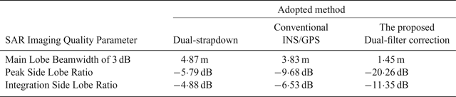
Table 5 shows the imaging quality parameters of azimuth direction, which are statistically calculated based on the response of scattering points and reflect the detailed quantitative analysis of SAR imaging effects based on the three INS/GPS methods. The MOCO with the dual-strapdown method has less accuracy, which is mainly displayed in main lobe beamwidth and peak side lobe ratio. Thus, the dual-strapdown method does not meet the MOCO requirements for SAR applications with long imaging periods. The MOCO results of the conventional INS/GPS method have a certain improvement but are not ideal. Compared with the two previous methods, the imaging quality based on the proposed dual-filtering correction method is obviously superior to that of the other two methods, and the azimuth resolution (approximately substituted by the main lobe beamwidth of 3 dB) reaches to 1·45 m and is the closest to the design value of 1 m.

Table 5.

SAR imaging quality parameters of azimuth direction.