1. Introduction
In actuarial science, the accurate determination of insurance premiums is of fundamental importance, as setting appropriate premiums directly affects both the financial stability of insurers and the economic welfare of policyholders. Within the field of non-life insurance, credibility theory has long been regarded as a cornerstone of premium calculation, providing a coherent and systematic framework for integrating historical experience with new observations through a credibility factor. By balancing individual experience with collective information, it enhances the accuracy, reliability, and stability of premium estimates and thereby occupies a central position in modern non-life pricing practice. Since its origin in the early twentieth century (Whitney, Reference Whitney1918; Bailey, Reference Bailey1945; Bühlmann, Reference Bühlmann1967), credibility theory has undergone continuous development and refinement over the past century. Owing to its flexibility in combining prior knowledge with observed data, it has also been widely applied beyond premium determination, including in loss reserving, risk portfolio evaluation, inequality measurement (such as Lorenz curves and Gini coefficients), and bibliometrics (Gisler and Wüthrich, Reference Gisler and Wüthrich2008; Pérez-Hornero, et al., Reference Pérez-Hornero, Arias-Nicolás, Pulgarín and Pulgarín2013; Wen et al., Reference Wen, Cao and Zhang2024), demonstrating its broad relevance for risk assessment and predictive modeling.
Classical credibility methods primarily focus on estimating hypothetical means (Bühlmann and Gisler, Reference Bühlmann and Gisler2005), which are sufficient for constructing premiums under the net premium and expected value principles. In practice, however, non-life insurers employ a variety of premium principles, including the variance principle, the standard deviation principle, and the modified variance premium principle (Teugels and Sundt, Reference Teugels and Sundt2004; Liang and Yuen, Reference Liang and Yuen2016; Zhang et al., Reference Zhang, Meng and Zeng2016; Sun et al., Reference Sun, Zheng and Zhang2017; Yong et al., Reference Yong, Zeng and Zhang2025). While the expected value principle is predominantly used in life insurance, the standard deviation principle is more common in non-life insurance, and the variance principle possesses several desirable theoretical properties that have been extensively studied in the literature (Bühlmann, Reference Bühlmann2007). The coexistence of these premium principles reflects the diversity of actuarial pricing methodologies and highlights the need for a unified framework capable of accommodating different premium calculation rules while fully leveraging the predictive power of credibility theory.
From a practical actuarial perspective, premium calculation must be aligned with the premium principles actually employed in insurance pricing. This consideration has motivated a strand of research that extends credibility theory beyond the classical net premium principle to alternative pricing rules. For instance, Wen et al. (Reference Wen, Wu and Zhao2009) derived credibility estimators under generalized weighted premium principles, Pan et al. (Reference Pan, Wang and Wu2008) examined the consistency of credibility premiums under the Esscher principle, and Wen et al. (Reference Wen, Wang and Wang2011) developed credibility premiums corresponding to the exponential principle.
Methodologically, these contributions are rooted in the decision-theoretic foundation of credibility theory (Heilmann, Reference Heilmann1989). The premium is reformulated as the solution to an optimization problem under a suitably specified loss function, so that the credibility premium emerges as an optimal linear Bayes estimator with respect to the prescribed loss structure. While this approach is effective for premium principles that admit a natural representation through loss function minimization, it becomes less suitable for pricing rules that cannot be directly characterized in this manner. In particular, variance-related premium principles—such as the variance principle, the standard deviation principle, and the modified variance principle, as well as their unified formulation, the variance-related premium principle (Guerra and de Lourdes Centeno, Reference Guerra and de Lourdes Centeno2010; Chi, Reference Chi2012; Zhang et al., Reference Zhang, Meng and Zeng2016)—do not readily fit into the classical loss-function-based credibility paradigm.
An important attempt to address this issue is due to Yong et al. (Reference Yong, Zeng and Zhang2025), who proposed a credibility pricing method under the variance principle by restricting the premium estimator to linear and quadratic functions of the sample observations and deriving the corresponding optimal linear Bayes estimator within this enlarged class. However, because the variance principle combines expectation and variance components measured on different scales, the resulting credibility estimator involves a comparatively complex structure and multiple structural parameters. Moreover, this construction is specifically tailored to the variance principle and does not extend naturally to other variance-related premium principles, such as the standard deviation principle, thereby limiting its general applicability.
Motivated by the aforementioned limitations, the present paper develops a unified framework for credibility estimation of the process variance under variance-related premium principles. In contrast to approaches that embed alternative premium principles into modified loss functions, we adopt a structurally different perspective by decoupling the estimation of the hypothetical mean from that of the process variance and focusing explicitly on the latter. Drawing inspiration from the normal–inverse gamma model with a known mean, we first derive the Bayesian estimator of the process variance, which can be expressed as a weighted combination of the sample variance and the prior variance, where the weights naturally exhibit a credibility interpretation: increasing reliance on sample information as the sample size grows and stronger dependence on prior information when data are limited. When the mean is unknown, we extend the framework by replacing the population mean with the sample mean, leading to a modified credibility estimator that preserves linearity and optimality in expectation. By combining this estimator with the classical credibility estimator of the hypothetical mean, we obtain credibility premiums for a broad class of variance-related premium principles. The resulting formulas are parsimonious, structurally transparent, and readily extendable, thereby enhancing both their theoretical coherence and practical applicability.
The contributions of this paper are fourfold. First, we show that directly applying the classical Bühlmann credibility estimator to process variance is inappropriate, revealing a limitation of existing credibility methods. Second, inspired by Bayesian linearization techniques, we construct new credibility estimators for process variance that are valid under both known and unknown hypothetical means. Third, we rigorously analyze the statistical properties of these estimators, including unbiasedness, mean squared error, consistency, and asymptotic normality. Fourth, by combining the proposed estimators of process variance with the classical Bühlmann credibility estimator for hypothetical means, we build a comprehensive framework for estimating risk premiums under a broad class of variance-related premium principles. Compared with existing methods such as Yong et al. (Reference Yong, Zeng and Zhang2025), our approach separates the estimation of mean and variance, requires fewer structural parameters, ensures numerical stability, and extends naturally to multiple premium principles. The practical performance and applicability of the proposed methodology are further illustrated through extensive simulations and an empirical analysis using real insurance claims data.
The remainder of the paper is organized as follows. Section 2 introduces the variance-related premium principles and their Bayesian formulations, provides a detailed review of classical credibility estimation methods for hypothetical means, and establishes the necessary and sufficient conditions for consistency in risk premium estimation. Section 3 develops credibility estimators for process variance under both known and unknown hypothetical means and rigorously investigates their finite-sample and asymptotic properties. Section 4 integrates the credibility estimators of both hypothetical means and process variance to construct a unified framework for risk premium estimation under variance-related premium principles and demonstrates the practical relevance of the proposed methods through numerical simulations and empirical analysis. Finally, Section 5 concludes the paper by summarizing the main findings and outlining potential directions for future research. To ensure the paper is fully self-contained, all proofs of the theoretical results are provided in a dedicated Appendix A.
2. Credibility estimators for variance-related premium principles
Credibility theory provides a framework for predicting future outcomes of individual risks by combining their own experience with the collective experience of a larger population. A risk X is assumed to depend on an underlying parameter
 $\Theta$
, which may be a scalar or a vector. For example, in automobile liability insurance,
 $\Theta$
may represent the combined effect of driver characteristics (age, gender, and behavior) and vehicle attributes (mileage, region, and engine type).
Since insurers generally lack full knowledge of all risk-influencing factors,
 $\Theta$
is modeled as a random variable or vector with prior distribution
 $\pi_{\Theta}(\theta)$
. Conditional on
 $\Theta=\theta$
, the observations
 $X_1,\ldots,X_n$
are assumed to be i.i.d. with distribution
 $f_{\theta}(x)$
. Under this structure, risk premium estimation naturally fits within the Bayesian framework. The model assumptions are summarized below:
Assumption A1. All factors influencing the risk X are represented by a random parameter
 $\Theta$
, with prior distribution
 $\pi_{\Theta}(\theta)$
.
Assumption A2. Given
 $\Theta=\theta$
, the samples
 $X_{1},\ldots,X_{n}$
are i.i.d. with common distribution
 $f_{\theta}(x)$
.
Here, the conditional expectation and conditional variance of X are denoted by
 \[\mu(\Theta) = \mathbb{E}(X|\Theta), \quad\gamma(\Theta) = \mathrm{Var}(X|\Theta),\]
which are referred to in actuarial science as the hypothetical mean and the process variance, respectively.
A model that satisfies Assumptions A1 and A2 is commonly referred to as a Bayesian model. In this setting, the risk associated with each individual is characterized by an underlying random parameter, and observed outcomes are assumed conditionally independent given this parameter. We focus on the problem of estimating credibility premiums under such a Bayesian framework, which allows the integration of individual claim experience with collective information from the broader population, providing a statistically coherent approach to premium determination.
Traditional credibility theory is typically grounded in the pure premium principle for premium pricing models (Teugels and Sundt, Reference Teugels and Sundt2004). Essentially, the pure premium principle considers only the expected value of the risk, without accounting for its volatility. In non-life insurance actuarial practice, incorporating variance components into the risk loading premium provides a more comprehensive and practical approach. Motivated by this idea, and building upon the variance-related premium principle introduced by Guerra and de Lourdes Centeno (Reference Guerra and de Lourdes Centeno2010), we extend their framework by defining the risk premium as a function of both the hypothetical mean and the process variance. Specifically, we define the risk premium under the variance-related premium principle as follows.
Definition 2.1. Under the Bayesian model, the risk premium based on the variance-related premium principle can be defined as
 \begin{equation}R\left( \Theta\right) = \mu(\Theta) + g\left(\mu(\Theta),\gamma(\Theta) \right) , \end{equation}
where g(x,y) is a continuous bivariate function.
In practice, the risk parameter
 $\Theta$
is typically unobservable, and thus the associated risk premium
 $R(\Theta)$
is also unknown and must be inferred from available data. To provide a rigorous foundation and clarify the estimation principle, we define the Bayesian premium under the squared loss criterion as follows. Specifically, the Bayesian premium is the measurable function of the sample that minimizes the expected squared loss between the estimator and the true (but unobservable) risk premium
 $R(\Theta)$
(Bühlmann and Gisler, Reference Bühlmann and Gisler2005).
Definition 2.2. Given a sample
 $\mathbf{X} = (X_1, \ldots, X_n)$
, the Bayesian premium of the risk
 $R(\Theta)$
is defined as its posterior expectation:
 \[\widehat{R_B(\Theta)} = \mathbb{E}[R(\Theta) \mid \mathbf{X}].\]
Equivalently, by decomposing
 $R(\Theta)$
into its mean and risk loading components, we have
 \[\widehat{R_B(\Theta)} = \mathbb{E}[\mu(\Theta) \mid \mathbf{X}] + \mathbb{E}[g(\mu(\Theta), \gamma(\Theta)) \mid \mathbf{X}].\]
If
 $\Theta$
is a continuous random variable, the Bayesian premium can be equivalently expressed in integral form as
 \begin{equation*}\widehat{R_B(\Theta)} =\frac{\displaystyle \int_{\Omega} \mu(\theta)\, \pi_{\Theta}(\theta) \prod_{i=1}^{n} f(x_i \mid \theta)\, d\theta}{\displaystyle \int_{\Omega} \pi_{\Theta}(\theta) \prod_{i=1}^{n} f(x_i \mid \theta)\, d\theta}+\frac{\displaystyle \int_{\Omega} g(\mu(\theta), \gamma(\theta)) \, \pi_{\Theta}(\theta) \prod_{i=1}^{n} f(x_i \mid \theta)\, d\theta}{\displaystyle \int_{\Omega} \pi_{\Theta}(\theta) \prod_{i=1}^{n} f(x_i \mid \theta)\, d\theta},\end{equation*}
where
 $(x_1, \ldots, x_n)$
denotes the observed sample corresponding to
 $(X_1, \ldots, X_n)$
, and
 $\Omega$
is the support of
 $\Theta$
.
Remark 2.1. To compute the Bayesian premium
 $\widehat{R_B(\Theta)}$
for a given loading function g(x,y), one must specify both the conditional distribution of the claim counts and the prior distribution of the underlying risk parameter. Consider the case where, conditional on
 $\Theta = \theta$
, the observations
 $X_1, \ldots, X_n$
are independent and identically distributed as
 $\text{Poisson}(\theta)$
, and the parameter
 $\Theta$
itself follows a
 $\mathrm{Gamma}(\alpha, \beta)$
distribution. By conjugacy, the posterior distribution of
 $\Theta$
remains Gamma with updated parameters
 $(\alpha+S, \beta+n)$
, where
 $S = \sum_{i=1}^{n} X_i$
denotes the total number of observed claims.
Under this specification, the hypothetical mean and process variance satisfy
 \[\mu(\Theta)=\gamma(\Theta)=\Theta,\qquad\mathbb{E}[\Theta \mid \mathbf{X}] = \frac{\alpha+S}{\beta+n}.\]
Since the general risk premium is defined in (2.1) and the Bayesian premium is the posterior expectation of
 $R(\Theta)$
, the estimator simplifies to
 \[\widehat{R_B(\Theta)}= \mathbb{E}[\Theta \mid \mathbf{X}]+ \mathbb{E}[g(\Theta,\Theta)\mid \mathbf{X}].\]
Therefore, the explicit formulas in the last column of Table 1 follow from evaluating the posterior expectation
 $\mathbb{E}[g(\Theta,\Theta)\mid \mathbf{X}]$
under the Gamma posterior distribution for each specified loading function g(x, y).
Examples of g(x, y), corresponding risk premiums, and Bayesian premiums.

Table 1 Long description
Panel A: Net premium with g(x, y) = 0, risk premium R0(Θ) = μ(Θ), and Bayesian premium (α+S)/(β+n). Panel B: Expected value with g(x, y) = ρ1·x, risk premium R1(Θ) = (1+ρ1)·μ(Θ), and Bayesian premium (1+ρ1)(α+S)/(β+n). Panel C: Variance premium with g(x, y) = ρ2·y, risk premium R2(Θ) = μ(Θ) + ρ2·γ(Θ), and Bayesian premium (1+ρ2)(α+S)/(β+n). Panel D: Standard deviation with g(x, y) = ρ3·√y, risk premium R3(Θ) = μ(Θ) + ρ3·√γ(Θ), and Bayesian premium (α+S)/(β+n) + ρ3Γ(α+S+1/2)/((β+n)^1/2Γ(α+S)). Panel E: Modified variance with g(x, y) = ρ4·y/x, risk premium R4(Θ) = μ(Θ) + ρ4·γ(Θ)/μ(Θ), and Bayesian premium (α+S)/(β+n) + ρ4.
The results in Table 1 indicate that, under the Poisson–Gamma model, the Bayesian premiums largely retain the functional form of their classical counterparts. This is because the risk parameter
 $\Theta$
is replaced by its posterior mean, and the loading term is adjusted through the corresponding posterior moments. For the net premium and the expected value premium, this substitution preserves their proportional relationship exactly. For more complex loading functions, such as the standard deviation premium, the Bayesian premiums include additional terms involving ratios of Gamma functions. These closed-form expressions demonstrate the analytical tractability of the Poisson–Gamma framework and clarify how different loading principles are modified under Bayesian estimation.
This remark shows that the Bayesian premium naturally blends individual experience with collective information, reflecting the core idea of credibility theory: assigning optimal weights to the individual and collective components to obtain a stable and equitable premium. In practice, however, the true conditional distribution
 $f_{\theta}(x)$
and prior
 $\pi_{\Theta}(\theta)$
are rarely known, making the Bayesian premium difficult to compute directly. To address this issue, Bühlmann (Reference Bühlmann1967) proposed restricting the estimator of
 $\mu(\Theta)$
to a linear function of the observations, leading to the classical linear credibility estimator. This provides a practical and interpretable alternative that preserves the essence of the Bayesian formulation.
By minimizing
 \[\mathbb{E}\Big[\big(\mu(\Theta) - a_0 - \sum_{i=1}^{n} a_i X_i \big)^2\Big],\]
the optimal linear Bayesian estimate of
 $\mu(\Theta)$
takes the standard credibility form
 \begin{equation}\widehat{\mu_C(\Theta)} = Z_n\,\overline{X}_n + (1-Z_n)\,\mu_0, \end{equation}
where
 $\overline{X}_n=\frac{1}{n}\sum_{i=1}^{n}X_i$
is the sample mean,
 $\mu_0=\mathbb{E}[\mu(\Theta)]$
is the collective mean, and
 \begin{equation}Z_n = \frac{n\,\mathrm{Var}[\mu(\Theta)]}{n\,\mathrm{Var}[\mu(\Theta)] + \mathbb{E}[\gamma(\Theta)]} \end{equation}
is the credibility factor. Bühlmann’s framework has become a cornerstone of non-life actuarial practice by providing a statistically sound method for combining individual and collective information.
However, classical Bühlmann credibility theory focuses solely on estimating the hypothetical mean
 $\mu(\Theta)$
. In many non-life insurance applications, premium principles depend not only on the mean but also on the process variance, as in variance-related premium principles (cf. (2.1)). Consequently, the traditional approach is insufficient when pricing methods also require accurate estimation of process variance, such as under the variance or standard deviation premium principles.
This paper focuses on the credibility estimation of process variance under the framework of credibility theory, aiming to provide a practical and theoretically grounded method for premium calculation across commonly used premium principles. To formalize the concept, we first introduce the definition of the credibility premium.
Definition 2.3. A credibility estimator systematically combines individual risk experience with collective information to estimate future premiums. Let
 $P_n$
denote the observed (experience-based) premium from a sample of size n, and
 $P_0$
denote the collective (aggregate) premium. The credibility estimator is defined as
 \[\widehat{P} = \xi(n) \cdot P_n + \big(1-\xi(n)\big) \cdot P_0,\]
where the credibility factor
 $\xi(n)$
satisfies
 $0 \le \xi(n) \le 1$
, increases with the sample size n, and approaches 1 as
 $n \to \infty$
. This formulation ensures a coherent and stable balance between individual and collective information.
Remark 2.2. The definition above provides a unified representation of credibility estimators across different settings. In particular, the relationship between the individual experience
 $P_n$
and the collective premium
 $P_0$
depends on whether the prior distribution is known:
-
(1) Prior distribution known (classical credibility): In this case,
 $P_0$
corresponds to the fixed prior mean of the risk parameter (Bühlmann Reference Bühlmann1967; Chen et al., Reference Chen, Cheung, Choi and Yam2020). The individual experience
$P_n$
is not included in
$P_0$
, and the two components can be treated as independent. The credibility estimator is then a linear approximation to the Bayesian premium under the known prior.
-
(2) Prior distribution unknown (empirical Bayes credibility): Here,
$P_0$
must be estimated from aggregated data, such as other policies in the portfolio or industry data (Mashayekhi, Reference Mashayekhi2002; Bühlmann and Gisler, Reference Bühlmann and Gisler2005; Zhang and Wen, Reference Zhang and Wen2024). The individual experience
$P_n$
may be included in the data used to estimate
$P_0$
, inducing statistical dependence between
$P_n$
and
$P_0$
. The credibility estimator remains a weighted average of the two components, but both are data-driven and potentially correlated.


In practical applications, such as launching a new line of business, the collective premium
 $P_0$
may be based on external industry data that exclude the individual insurer’s own experience. In these cases, the individual and collective components can again be treated as independent.
This remark clarifies that Definition 2.3 does not assume
 $P_n$
must be included in
 $P_0$
; rather, the inclusion or exclusion depends on the specific setting. The subsequent theorems and methodology apply to all these scenarios, with appropriate consideration of independence or dependence between
 $P_n$
and
 $P_0$
.
Building on the unified credibility framework presented above, we next apply the classical Bühlmann methodology. Specifically, by constraining the risk premium estimate to be a linear function of the observed sample, we obtain the optimal linear Bayesian estimate of the risk premium, as formalized in the following theorem.
Theorem 2.1. Under the variance premium principle, the optimal linear Bayesian estimation of the risk premium
 $R(\Theta)$
is obtained by solving:
 \[\min_{b_{0},b_{1},\ldots,b_{n}\in\mathbb{R}}\mathbb{E}\left[\left( R(\Theta)-b_{0}-\sum_{i=1}^{n}b_{i}X_{i}\right) ^{2}\right] ,\]
which is given by:
 \begin{equation}\widehat{R_C(\Theta)}=T_{n}\overline{X}_n+\left( 1-\frac{T_{n}\mu_{0}}{R_{0}}\right) R_{0},\end{equation}
where
 $R_{0}=\mathbb{E}[R(\Theta)]$
,
 $\tau^{2}=\mathrm{Var}[\mu(\Theta)]$
,
 $\varphi=\mathrm{Cov}(R(\Theta),\mu(\Theta))$
,
 $\sigma^{2}=\mathbb{E}[\mathrm{Var}(X|\Theta)]$
, and
 \[T_{n}=\frac{n\varphi}{n\tau^{2}+\sigma^{2}}.\]
Here,
 $\mathrm{Cov}(R(\Theta),\mu(\Theta))$
indicates the covariance between
 $R(\Theta)$
and
 $\mu(\Theta)$
.
The proof of Theorem 2.1 is provided in Appendix A.1. From this result, the optimal linear Bayesian estimator
 $\widehat{R_C(\Theta)}$
admits a credibility-like weighted representation, in which the factor
 $T_n$
plays a role analogous to that of a classical credibility factor. However, in contrast to standard credibility estimators, the resulting weights do not necessarily form a convex combination. More importantly,
 $\widehat{R_C(\Theta)}$
is, in general, not consistent for the true risk premium
 $R(\Theta)$
. Consequently, in most practical settings, this estimator cannot be reliably interpreted as a credibility-based premium.
Theorem 2.2. The optimal linear Bayesian estimator
 $\widehat{R_C(\Theta)}$
is consistent with respect to
 $R(\Theta)$
if and only if there exist constants s and t such that
 \[g\big(\mu(\Theta),\gamma(\Theta)\big) = s\,\mu(\Theta) + t.\]
Theorem 2.2 reveals an important structural implication for the linear Bayesian estimator
 $\widehat{R_C(\Theta)}$
defined in Theorem 2.1. In order for
 $\widehat{R_C(\Theta)}$
to be consistent with respect to
 $R(\Theta)$
, the loading function
 $g(\mu(\Theta),\gamma(\Theta))$
must be linear in the hypothetical mean
 $\mu(\Theta)$
.
This condition implies that the resulting premium principle effectively reduces to the expected premium principle. Consequently, the linear estimator in Theorem 2.1 does not provide a genuine generalization of commonly used premium principles. In particular, many variance-based loading functions widely used in actuarial practice do not satisfy this linearity requirement, and therefore the estimator
 $\widehat{R_C(\Theta)}$
will generally not be consistent under such premium principles.
This limitation motivates the development of the alternative credibility estimation methods presented in Section 3, which are designed to ensure consistent premium estimation while accommodating more general premium principles. The proof of Theorem 2.2 is provided in Appendix A.2.
Remark 2.3. The structural parameters appearing in Theorem 2.1, namely
 $R_{0}$
,
 $\tau^{2}$
,
 $\varphi$
, and
 $\sigma^{2}$
, can be estimated using a fully nonparametric approach. This procedure relies solely on the empirical moments of the observed data and does not require any specific distributional assumptions on the latent risk parameter
 $\Theta$
. Accordingly, it provides a flexible and model-free framework for approximating the underlying structure of the premium model.
Suppose that m independent risk units are observed, with the ith unit containing
 $n_i$
realizations
 $X_{ij}$
 $(j=1,\ldots,n_i)$
. It should be noted that the credibility estimators described above are not the ones recommended in this paper, as they often fail to yield consistent estimates (c.f. Theorem 2.2). For simplicity, we focus here on estimating the hyperparameters of the balanced model, where
 $n_1 = n_2 = \cdots = n_m = n$
. For a detailed discussion on hyperparameter estimation in unbalanced models, the reader is referred to Bühlmann and Gisler (Reference Bühlmann and Gisler2005).
For each risk unit i
 $(i=1,2,\ldots ,m)$
, we define the sample mean and sample variance as
 \begin{equation*}\overline{X}_{n_{i}}=\frac{1}{n}\sum_{j=1}^{n}X_{ij},\qquad S_{n_{i}}^{2}=\frac{1}{n-1}\sum_{j=1}^{n}(X_{ij}-\overline{X}_{n_{i}})^{2}.\end{equation*}
These statistics serve as empirical estimates of the latent parameters
 $\mu(\Theta _{i})$
and
 $\gamma (\Theta _{i})$
, respectively, and constitute the fundamental quantities for subsequent nonparametric estimation of the structural parameters.
The structural parameters can then be estimated by
 \begin{equation*}\hat{R}_{0}=\frac{1}{m}\sum_{i=1}^{m}\big[\overline{X}_{n_{i}}+g\big(\overline{X}_{n_{i}},S_{n_{i}}^{2}\big)\big],\quad \hat{\sigma}^{2}=\frac{1}{m}\sum_{i=1}^{m}S_{n_{i}}^{2},\quad \hat{\tau}^{2}=\frac{1}{m-1}\sum_{i=1}^{m}(\overline{X}_{n_{i}}-\bar{\mu})^{2}-\frac{1}{n}\hat{\sigma}^{2},\end{equation*}
and
 \begin{equation*}\hat{\varphi}=\frac{1}{m-1}\sum_{i=1}^{m}\big[\big(\overline{X}_{n_{i}}+g\big(\overline{X}_{n_{i}},S_{n_{i}}^{2}\big)\big)-\hat{R}_{0}\big](\overline{X}_{n_{i}}-\bar{\mu}),\end{equation*}
where
 $\bar{\mu}=\frac{1}{m}\sum_{i=1}^{m}\overline{X}_{n_{i}}$
represents the overall sample mean across all risk units.
This nonparametric estimation framework accommodates any continuous specification of the function g(x, y), including
 $g(x,y) = 0$
,
 $g(x,y) =\rho_1 x$
,
 $g(x,y) = \rho_2 y$
,
 $g(x,y) = \rho_2 \sqrt{y}$
, and
 $g(x,y) =\rho \, \frac{y}{x}$
(see Table 1). This flexibility ensures broad applicability and practical relevance across a wide range of variance-related premium principles.
3. New credibility estimation of process variance
3.1 Known mean case
In the variance-related premium principle, the risk premium is primarily composed of two components: the hypothetical mean
 $\mu(\Theta)$
and the process variance
 $\gamma(\Theta)$
. While the credibility estimate for the hypothetical mean has been extensively studied (c.f. (2.2)), obtaining a reliable estimate for the process variance component is equally crucial for accurate risk premium calculation.
Let
 $X_{1},\ldots,X_{n}$
denote independent and identically distributed (i.i.d.) samples conditional on the parameter
 $\Theta$
, and let
 $\gamma(\Theta) = \mathrm{Var}(X_1 |\Theta)$
represent the conditional variance of the population. Under the squared-error loss criterion, the optimal estimator of
 $\gamma(\Theta)$
is the posterior mean in the Bayesian framework:
 \begin{equation} \widehat{\gamma_B(\Theta)} = \mathbb{E}[\gamma(\Theta) \mid X_1,\ldots,X_n],\end{equation}
which serves as the Bayesian estimator of the process variance. In specific models, this Bayesian estimator can be expressed in a form equivalent to the classical credibility formula, demonstrating the close connection between Bayesian estimation and credibility theory.
The following example illustrates the Bayesian estimation of the process variance in the normal distribution case, showing how credibility theory can be applied in practical scenarios.
Example 3.1. Consider the case where, conditional on
 $\Theta = \theta$
, the observations
 $X_1, \ldots, X_n$
are independent and identically distributed as
 $N(\mu_0, \theta)$
, and the process variance parameter
 $\Theta$
itself follows an inverse gamma distribution
 $\mathrm{IG}(\alpha, \beta)$
. The conditional density of
 $X_i$
given
 $\Theta = \theta$
is
 \begin{equation*}f_{\theta}(x) = \frac{1}{\sqrt{2\pi \theta}} \exp\Big\{-\frac{(x-\mu_0)^2}{2\theta}\Big\},\end{equation*}
while the prior density of
 $\Theta$
is
 \begin{equation*}\pi_{\Theta}(\theta) = \frac{\beta^{\alpha}}{\Gamma(\alpha)} \theta^{-(\alpha+1)} e^{-\beta/\theta}.\end{equation*}
By Bayes’ theorem, the posterior distribution of
 $\Theta$
given the observed sample is
 \begin{equation*}\left[\Theta \mid X_1, \ldots, X_n \right] \sim \mathrm{IG}\Big(\alpha + \frac{n}{2}, \, \beta + \frac{1}{2} \sum_{i=1}^{n} (X_i - \mu_0)^2 \Big),\end{equation*}
which belongs to the inverse gamma conjugate family (see, e.g., Gelman et al. Reference Gelman, Carlin, Stern, Dunson, Vehtari and Rubin2013). The corresponding Bayesian estimator of the process variance is
 \begin{equation*}\widehat{\gamma_B(\Theta)} = \frac{\beta + \frac{1}{2}\sum_{i=1}^{n} (X_i - \mu_0)^2}{\alpha + \frac{n}{2} - 1}.\end{equation*}
This Bayesian estimator can equivalently be expressed in the standard credibility form:
 \begin{equation*}\widehat{\gamma_B(\Theta)} = w_n S_n^2 + (1 - w_n) \gamma_0,\end{equation*}
where
 \begin{equation*}S_n^2 = \frac{1}{n} \sum_{i=1}^{n} (X_i - \mu_0)^2, \quad\gamma_0 = \frac{\beta}{\alpha - 1}, \quad w_n = \frac{n}{n + 2(\alpha - 1)}.\end{equation*}
The posterior variance of
 $\gamma(\Theta)$
is given by
 \begin{equation*}\mathrm{Var}[\gamma(\Theta) \mid X_1, \ldots, X_n] = \frac{\left(\beta + \frac{n}{2} S_n^2\right)^2}{\left(\alpha + \frac{n}{2} - 1\right)^2 \left(\alpha + \frac{n}{2} - 2\right)}.\end{equation*}
Remark 3.1. Note that, for
 $\Theta \sim \mathrm{IG}(\alpha, \beta)$
, the mean and variance are given by
 \begin{equation*}\mathbb{E}[\Theta] = \frac{\beta}{\alpha - 1}, \qquad\mathrm{Var}(\Theta) = \frac{\beta^2}{(\alpha - 1)^2 (\alpha - 2)}, \quad \alpha \gt 2.\end{equation*}
Hence, the posterior variance of the process variance
 $\gamma(\Theta)$
is well-defined only when
 $\alpha \gt 2$
.
Furthermore, the marginal distribution of each
 $X_i$
can be derived by integrating out
 $\Theta$
:
 \begin{align*}f_{X_{i}}(x)& =\int_{0}^{\infty }\frac{1}{\sqrt{2\pi \theta }}\exp \Big\{-\frac{(x-\mu _{0})^{2}}{2\theta }\Big\}\frac{\beta ^{\alpha }}{\Gamma(\alpha )}\theta ^{-(\alpha +1)}e^{-\beta /\theta }\,d\theta \\[5pt] & =\frac{\Gamma \!\left( \alpha +\frac{1}{2}\right) }{\Gamma (\alpha )\sqrt{2\pi \beta }}\left[ 1+\frac{(x-\mu _{0})^{2}}{2\beta }\right] ^{-(\alpha+1/2)}.\end{align*}
This is precisely a Student’s t-distribution with
 $2\alpha$
degrees of freedom, location parameter
 $\mu_0$
, and scale parameter
 $\sqrt{\beta/\alpha}$
, that is,
 \begin{equation*}X_i \sim t_{2\alpha} \big(\mu_0, \sqrt{\beta/\alpha} \big).\end{equation*}
This derivation explicitly shows how the heavy-tailed Inverse-Gamma prior for
 $\Theta$
induces a Student’s t-marginal distribution for
 $X_i$
, providing robustness in modeling and inference.
In Example 3.1, the weight
 $w_n$
plays a central role in determining the posterior mean estimator
 $\widehat{\Theta}_B$
of the process variance parameter
 $\Theta$
. It quantifies the relative influence of the sample variance
 $S_n^2$
on
 $\widehat{\Theta}_B$
compared to the prior mean
 $\mathbb{E}[\Theta] = \beta / (\alpha - 1)$
. It is straightforward to verify that
 $w_n \to 1$
as
 $n \to \infty$
and
 $w_n \to 0$
as
 $n \to 0$
. Consequently, for large sample sizes, the Bayesian estimator
 $\widehat{\Theta}_B$
is primarily driven by the observed data through
 $S_n^2$
, making it largely data-driven. In contrast, for small n,
 $w_n$
is smaller, and the prior mean exerts greater influence, reflecting the more significant role of prior information when observations are limited.
The weight
 $w_n$
therefore balances the contributions of the observed data and the prior information, allowing
 $\widehat{\Theta}_B$
to smoothly transition from reliance on the prior under scarce data conditions to reliance on the sample information as the number of observations increases. This property ensures a robust estimation procedure that accounts for both data variability and prior knowledge (Bühlmann, Reference Bühlmann1967; Bühlmann and Gisler, Reference Bühlmann and Gisler2005; Zhang, Reference Zhang2023).
In practical insurance applications, the conditional distribution of the population and the distribution of the risk parameter are often unknown, which generally prevents exact Bayesian computations. While the example in Example 3.1 is specific and admits an explicit solution only under conjugate assumptions, it provides useful insight: Bayesian estimation of conditional parameters can be interpreted as a weighted combination of the sample variance and the prior mean of the process variance, closely aligning with the principles of traditional credibility theory.
To better utilize the principles of credibility theory for obtaining credibility estimates of process variance
 $\gamma(\Theta)$
, we assume that the hypothetical mean
 $\mu(\Theta)$
is known, that is,
 $\mu(\Theta) = \mu_{0}$
, and solve the following minimization problem:
 \begin{equation}\min_{a_{0}, a_{1}, \ldots, a_{n} \in\mathbb{R}} \mathbb{E}\left[ \left(\gamma(\Theta) - a_{0} - \sum_{i=1}^{n} a_{i} \left( X_{i} - \mu_{0} \right)^{2} \right) ^{2} \right] . \end{equation}
The objective of the optimization problem (3.2) is to construct a linear estimator for the process variance
 $\gamma(\Theta)$
by minimizing the expected squared deviation between
 $\gamma(\Theta)$
and a linear combination of the squared deviations
 $(X_i - \mu_0)^2$
. This formulation is equivalent to the classical credibility problem applied to the transformed variable
 $Y_i = (X_i - \mu_0)^2$
, where the estimation focus is shifted from the original observations
 $X_i$
to their squared deviations.
To characterize the statistical structure of this problem, let
 $Y_i = (X_i - \mu_0)^2$
for
 $i = 1, \ldots, n$
. Then,
 $Y_1, \ldots, Y_n$
are conditionally independent and identically distributed given
 $\Theta$
, with
 \[\mathbb{E}(Y_i|\Theta) = \gamma(\Theta), \quad\mathrm{Var}(Y_i|\Theta) = k_4(\Theta) - \gamma^2(\Theta),\]
where
 $k_4(\Theta) = \mathbb{E}[(X_1 - \mu_0)^4|\Theta]$
. Taking expectations with respect to
 $\Theta$
yields
 \[\mathbb{E}[\mathrm{Var}(Y_i|\Theta)] = k_4 - \lambda - \gamma_0^2 = v,\]
where
 $k_4=\mathbb{E}[k_4(\Theta)]$
,
 $\lambda = \mathrm{Var}[\gamma(\Theta)]$
and
 $\gamma_0 = \mathbb{E}[\gamma(\Theta)]$
.
According to the standard methods in credibility theory (Bühlmann, Reference Bühlmann1967; Bühlmann and Gisler, Reference Bühlmann and Gisler2005), the optimal linear credibility estimator in this setting is a weighted combination of the sample variance and the collective variance, with the weight determined by the relative magnitudes of the within-group and between-group variances. Consequently, we obtain the following corollary.
Corollary 3.1. Under Assumptions A1 and A2 of the Bayesian model, if
 $\mu(\Theta) = \mu_0$
, the optimal estimator of the process variance
 $\gamma(\Theta)$
obtained by solving (3.2) is given by
 \begin{equation}\widehat{\gamma_C(\Theta)}= w_n^{\ast} S_n^2 + \left(1 - w_n^{\ast}\right) \gamma_0,\end{equation}
where
 $\gamma_0 = \mathbb{E}[\gamma(\Theta)]$
denotes the collective (a priori) variance,
 $S_n^2 = \frac{1}{n} \sum_{i=1}^{n} (X_i - \mu_0)^2$
is the sample variance, and
 \begin{equation}w_n^{\ast} = \frac{n\lambda}{n\lambda + v}\end{equation}
is the credibility factor.
This corollary establishes a Bayesian–credibility framework for estimating the process variance
 $\gamma(\Theta)$
. The result shows that the optimal estimator is a weighted average of the sample variance
 $S_n^2$
and the collective variance
 $\gamma_0$
, with the credibility factor
 $w_n^{\ast}$
reflecting the relative importance of the observed data and the prior information. Specifically,
 $w_n^{\ast}$
depends on the ratio between the between-group variance
 $\lambda$
and the within-group variance v and increases with the sample size n. Hence, as more data become available, the estimator increasingly relies on the empirical sample variance, while for smaller samples, the estimation remains more influenced by the prior collective information.
This balance between prior belief and observed data lies at the core of credibility theory, providing a natural Bayesian interpretation of the credibility premium principle. Moreover, the formulation ensures that the estimator
 $\widehat{\gamma_C(\Theta)}$
is unbiased and efficient under the assumed conditional independence and distributional conditions, highlighting its practical relevance in actuarial science and risk management.
Remark 3.2. In Example 3.1, under the normal model with known mean and an inverse-gamma prior, the Bayesian estimator of the process variance admits the linear representation
 \[\widehat{\gamma_B(\Theta)}=w_n S_n^2 + (1-w_n)\gamma_0,\]
which coincides exactly with the credibility estimator in Corollary 3.1. This agreement is structural rather than accidental. In the normal model with known mean, the variance parameter
 $\Theta$
is itself the scale parameter, and the likelihood depends on
 $\Theta$
only through the quadratic sufficient statistic
 $\sum_{i=1}^n (X_i-\mu_0)^2$
. The inverse-gamma prior is conjugate with respect to this quadratic structure, so posterior updating simply modifies the hyperparameters via functions of
 $\sum_{i=1}^n (X_i-\mu_0)^2$
. Consequently, the posterior mean
 $\mathbb{E}[\Theta\mid X_1,\ldots,X_n]$
is an affine function of
 $S_n^2$
, yielding an exact credibility-type formula.
In contrast, for a general one-parameter exponential family with conjugate prior, the process variance
 $\gamma(\Theta)=\mathrm{Var}(X_1\mid\Theta)$
is typically a nonlinear function of the structural parameter
 $\Theta$
. Although conjugacy ensures analytical tractability of the posterior distribution of
 $\Theta$
, it does not guarantee that the posterior mean
 $\mathbb{E}[\gamma(\Theta)\mid X_1,\ldots,X_n]$
can be expressed as a linear function of quadratic statistics such as
 $S_n^2$
. Unless the variance parameter coincides directly with the canonical scale parameter and the sufficient statistic has a purely quadratic form, such an exact credibility representation generally fails.
Nevertheless, this lack of exact equivalence does not diminish the relevance of the credibility estimator. The estimator derived from (3.2) is the optimal predictor within the class of linear estimators under squared-error loss. Hence, even when the Bayesian estimator is not exactly linear, the credibility estimator can be interpreted as its best linear approximation, depending only on low-order moment quantities
 $(\gamma_0,\lambda,v)$
. This moment-based structure provides robustness and computational simplicity, making the credibility approach a practically attractive alternative when full distributional specification is uncertain or when conjugacy does not preserve linearity.
A systematic characterization of the distribution–prior combinations under which the Bayesian estimator of the process variance admits an exact credibility-type linear representation remains an interesting open problem beyond the scope of the present paper.
Remark 3.3. The credibility estimator
 $\widehat{\gamma_C(\Theta)}$
is unconditionally unbiased for
 $\gamma_0$
in the sense that
 \[\mathbb{E}\big[\widehat{\gamma_C(\Theta)}\big]= w_n^\ast \, \mathbb{E}\big[S_n^2\big] + (1-w_n^\ast)\gamma_0= w_n^\ast \gamma_0 + (1-w_n^\ast)\gamma_0= \gamma_0 = \mathbb{E}\big[\gamma(\Theta)\big].\]
Its unconditional mean squared error can be written as
 \begin{align*}\mathrm{MSE}\big(\widehat{\gamma_C(\Theta)}\big)&= (w_n^\ast)^2 \, \mathbb{E}\big[(S_n^2 - \gamma(\Theta))^2\big]+ (1-w_n^\ast)^2 \, \mathbb{E}\big[(\gamma_0 - \gamma(\Theta))^2\big]\\[5pt] &\quad + 2 w_n^\ast (1-w_n^\ast) \, \mathbb{E}\big[\big(S_n^2 - \gamma(\Theta)\big)(\gamma_0 - \gamma(\Theta))\big].\end{align*}
Since
 $\mathbb{E}[S_n^2 \mid \Theta] = \gamma(\Theta)$
, the cross term vanishes:
 $\mathbb{E}[(S_n^2 - \gamma(\Theta))(\gamma_0 - \gamma(\Theta))] = 0.$
Hence, the unconditional MSE simplifies to
 \[\mathrm{MSE}\big(\widehat{\gamma_C(\Theta)}\big)= (w_n^\ast)^2 \, \mathbb{E}\big[\mathrm{Var}\big(S_n^2 \mid \Theta\big)\big]+ (1-w_n^\ast)^2 \lambda= \lambda (1-w_n^\ast)= w_n^\ast \frac{v}{n},\]
where v denotes the variance of
 $S_n^2$
and
 $\lambda$
the prior variance of
 $\gamma(\Theta)$
. It follows that
 $\mathrm{MSE}\big(\widehat{\gamma_C(\Theta)}\big) \to 0$
as
 $n \to \infty$
.
Furthermore, we can prove the consistency and asymptotic normality of the credibility estimation.
Theorem 3.1. Given
 $\Theta,$
the estimator
 $\widehat{\gamma_C(\Theta)}$
is consistent and asymptotically normal. Specifically, the following results hold:
-
(1)
$\widehat{\gamma_C(\Theta)}\overset{a.s.}{\rightarrow}\gamma(\Theta)$
as
$n\rightarrow\infty$
; -
(2)
$\sqrt{n}\left[ \widehat{\gamma_C(\Theta)}-\gamma(\Theta)\right] \overset{d}{\rightarrow}\mathcal{N}\left( 0,\sigma_{\gamma}^{2}\left( \Theta\right) \right) $
as
$n\rightarrow\infty$
, where
$\sigma_{\gamma}^{2}\left( \Theta\right) =k_{4}\left( \Theta\right)-\gamma^{2}(\Theta)$
is the conditional asymptotic variance.


The proof is provided in Appendix A.3. This theorem establishes the large-sample properties of
 $\widehat{\gamma_C(\Theta)}$
under a fixed risk parameter
 $\Theta$
. The almost sure consistency ensures convergence to the true process variance, while asymptotic normality provides a basis for statistical inference in large samples. Together, these results justify the use of the proposed credibility estimator in practical applications where the sample size is moderate to large.
As discussed in Remark 3.2, we consider a hierarchical model in which, conditional on
 $\Theta = \theta$
, the observations
 $X_1, \ldots, X_n$
are i.i.d.
 $N(\mu_0, \theta)$
.
To explore the performance of the credibility estimator beyond conjugacy, we now replace the inverse-gamma prior with a non-conjugate specification. The results show that, even without a conjugate prior, the credibility estimator remains well-defined and closely approximates the Bayesian estimator, providing a practical and accurate alternative in such settings.
Example 3.2. Consider a hierarchical model in which, conditional on
 $\Theta = \theta$
, the observations
 $X_1, \ldots, X_n$
are i.i.d.
 $N(\mu_0, \theta)$
, and the prior distribution of
 $\Theta$
is
 $\mathrm{Gamma}(\alpha, \beta)$
with
 $\alpha, \beta \gt 0$
.
Under this model, we have
 $\gamma(\Theta) = \Theta$
. Moreover,
 \[\mathbb{E}\big[(X_i - \mu_0)^2 \mid \Theta\big] = \Theta,\qquad\mathrm{Var}\big((X_i - \mu_0)^2 \mid \Theta\big) = 2\Theta^2.\]
It follows that the structural parameters in the credibility framework are
 \[\gamma_0 = \mathbb{E}[\Theta] = \frac{\alpha}{\beta}, \quad\lambda = \mathrm{Var}(\Theta) = \frac{\alpha}{\beta^2}, \quad v = \mathbb{E}[2\Theta^2] = \frac{2\alpha(1+\alpha)}{\beta^2}.\]
The resulting credibility estimator is
 \[\widehat{\gamma_C(\Theta)} = w_n^{\ast} S_n^2 + (1 - w_n^{\ast}) \gamma_0,\quad w_n^{\ast} = \frac{n}{n + 2(1+\alpha)}.\]
Since the Gamma prior is not conjugate to the normal likelihood with known mean, the posterior distribution of
 $\Theta$
is not available in closed form. Consequently, the Bayesian estimator
 $\widehat{\gamma_B(\Theta)} =\mathbb{E}[\Theta \mid X_1, \ldots, X_n]$
is no longer an affine function of
 $S_n^2$
and must be evaluated numerically.
In contrast, the credibility estimator remains explicit and depends only on the low-order moments
 $(\gamma_0, \lambda, v)$
. To quantify the discrepancy between the Bayesian and credibility approaches, we consider the unconditional mean squared error (MSE),
 \begin{equation}\mathrm{MSE}\big(\widehat{\gamma_v(\Theta)}\big)= \mathbb{E}\Big[\big(\widehat{\gamma_v(\Theta)} - \gamma(\Theta)\big)^2\Big],\quad v \in \{B, C\},\end{equation}
which is evaluated via Monte Carlo simulation.
Figure 1 reports the simulated MSEs under different sample sizes. For all values of n, the Bayesian estimator exhibits a slightly lower MSE than the credibility estimator. However, the difference remains modest. As the sample size increases, the gap further diminishes and becomes negligible for moderate to large samples (e.g.,
 $n \geq 100$
), indicating that the credibility estimator provides an accurate approximation to the Bayesian estimator in such settings.
Unconditional mean squared error of the Bayesian and credibility estimators for different sample sizes.

To further investigate the distributional behavior of the Bayesian and credibility estimators at a fixed value of
 $\Theta = 1.5$
, we examine QQ-plots for two representative sample sizes,
 $n=30$
and
 $n=100$
. These plots allow us to visually assess how closely the empirical distributions of the two estimators align and to evaluate their approximate normality.
Figure 2 shows that the points are approximately aligned along the diagonal for both sample sizes, indicating that the Bayesian and credibility estimators are nearly normally distributed. Mild deviations are observed for
 $n=30$
, reflecting finite-sample differences, while for
 $n=100$
the points lie closer to the diagonal, demonstrating increasingly similar distributions and supporting their asymptotic normality.
QQ-plots of the Bayesian and credibility estimators at
 $\Theta = 1.5$
for
 $n=30$
(left) and
 $n=100$
(right).

Example 3.2 highlights several important features arising in the non-conjugate setting. First, while the credibility estimator of the process variance retains an explicit closed-form expression, the corresponding Bayesian estimator is no longer analytically tractable and must be evaluated numerically, for instance via simulation-based methods.
Second, despite the loss of conjugacy, the credibility estimator continues to provide a close approximation to the Bayesian estimator. This is supported by the simulation results, which show that the two estimators have very similar mean squared errors, with only minor differences even for moderate sample sizes.
Finally, from a distributional perspective, both estimators exhibit asymptotic normality. As the sample size n increases, their empirical distributions become increasingly similar, further confirming that the credibility estimator serves as an accurate and computationally efficient proxy for the Bayesian estimator in large samples.
3.2 Unknown mean case
In the previous subsections, we considered the estimation of the process variance
 $\gamma(\Theta)$
under the assumption that the hypothetical mean
 $\mu(\Theta)$
is known. However, in many practical situations, this assumption does not hold, and the hypothetical mean must be estimated jointly with the process variance. This joint estimation increases the complexity of the risk premium evaluation
 $R(\Theta)$
, since both the mean and the variance must be inferred from the available data.
Nevertheless, the Bühlmann credibility estimator
 $\widehat{\mu_{C}(\Theta)}$
in (2.2) already provides an optimal estimator of the hypothetical mean when the prior distribution is unknown. Therefore, in the context of variance-related premium principles, we will not further address the estimation of
 $\mu(\Theta)$
. Instead, we directly substitute its Bühlmann credibility estimate when required. Our primary focus remains on developing a credibility estimator for the process variance
 $\gamma(\Theta)$
.
Different from the previous subsection, when the hypothetical mean is unknown, the key idea is to replace the term
 $(X_i - \mu_0)^2$
with its centered counterpart
 $(X_i - \overline{X}_n)^2$
, where
 $\overline{X}_n$
is the sample mean. To formalize this approach, we introduce the following quantities:
 \[u_{4}(\Theta)= \mathbb{E}\!\left[\left.(X_1 - \mu(\Theta))^4\right|\Theta\right], \qquad\delta_{n}(\Theta)= \mathrm{Var}\big[\tilde{S}_n^2\big|\Theta\big], \qquad\delta_{n}= \mathbb{E}\!\left[\delta_{n}(\Theta)\right],\]
where
 $\tilde{S}_n^2 = \frac{1}{n-1} \sum_{i=1}^{n} (X_i - \overline{X}_n)^2$
denotes the unbiased sample variance. Here, the quantity
 $\lambda$
appearing later in Theorem 3.2 refers to the between-group variability of the process variance
 $\gamma(\Theta)$
, as defined previously. The above notation summarizes the conditional fourth central moment and the conditional and unconditional variability of
 $\tilde{S}_n^{2}$
, which play a key role in the derivation of the credibility estimator for the unknown mean case.
This leads to the following theorem, which generalizes the credibility estimation of the process variance to the case of an unknown hypothetical mean.
Theorem 3.2. Under the Bayesian model with unknown mean
 $\mu(\Theta)$
, the optimal linear estimator of the process variance
 $\gamma(\Theta)$
is obtained by solving
 \begin{equation}\min_{a_{0},a_{1},\ldots,a_{n}\in\mathbb{R}}\mathbb{E}\!\left[\left(\gamma(\Theta)- a_{0}- \sum_{i=1}^{n} a_{i} (X_i - \overline{X}_n)^2\right)^{2}\right].\end{equation}
The solution is given by the credibility-weighted estimator
 \begin{equation}\widetilde{\gamma_C(\Theta)}= t_{n}^{\ast}\, \tilde{S}_n^{2}+ (1 - t_{n}^{\ast})\, \gamma_{0},\end{equation}
where
 $\tilde{S}_n^2$
is the unbiased sample variance of the observations,
 $\gamma_{0} = \mathbb{E}[\gamma(\Theta)]$
denotes the collective (a priori) variance,
 $\lambda = \mathrm{Var}[\gamma(\Theta)]$
is the between-group variance of the process variance, and
 $t_{n}^{\ast} = \frac{\lambda}{\lambda + \delta_{n}}$
is the credibility factor balancing the individual sample variance and the collective variance.
The proof of Theorem 3.2 is provided in Appendix A.4. This result extends the classical credibility framework to the case where the hypothetical mean is unknown. By using the centered observations
 $(X_i - \overline{X}_n)^2$
, the estimator retains its interpretability and computational simplicity, while effectively adjusting for the uncertainty introduced by estimating the mean. As in the known-mean case, the credibility factor
 $t_{n}^{\ast}$
reflects the relative weight assigned to the observed sample variance and the collective (prior) variance, ensuring a balanced integration of empirical data and prior structure.
Remark 3.4. By evaluating the conditional expectation and fourth-order moment of
 $\tilde{S}_n^2$
given
 $\Theta$
under the hierarchical framework (Benhamou, Reference Benhamou2018), we have
 \[\delta_{n}(\Theta) = \mathrm{Var}\big(\tilde{S}_n^2 \mid \Theta\big)= \frac{u_4(\Theta)}{n} - \frac{n-3}{n(n-1)} \,\gamma^2(\Theta),\]
and its unconditional expectation
 \[\delta_n = \mathbb{E}[\delta_n(\Theta)]= \frac{u_4}{n} - \frac{(n-3)(\lambda+\gamma_0^2)}{n(n-1)}= \frac{1}{n} (u_4 - \lambda - \gamma_0^2) + \frac{2(\lambda+\gamma_0^2)}{n(n-1)}.\]
Consequently, the credibility factor can be expressed as
 \[t_n^* = \frac{\lambda}{\lambda + \delta_n}= \frac{n}{\,n + \kappa_n\,},\]
where
 $\kappa_n = (u_4 - \lambda - \gamma_0^2)/\lambda + 2\,(\lambda + \gamma_0^2)/[\lambda (n-1)]$
is a constant of order O(1) with respect to n.
This form explicitly shows the dependence of
 $t_n^*$
on the sample size n:
 $t_n^*$
increases with n and approaches 1 as
 $n\to\infty$
. Intuitively, as the sample size grows, the credibility estimator gives more weight to the sample component and less to the prior, whereas for small n, the prior receives more weight, consistent with standard credibility theory.
Remark 3.5. The credibility estimation
 $\widetilde{\gamma_C(\Theta)}$
is an unconditionally unbiased estimator of
 $\gamma_{0}$
in the sense of
 $\mathbb{E}\left[ \widetilde{\gamma_C(\Theta)}\right] =\mathbb{E}\left[\gamma(\Theta)\right] =\gamma_{0}.$
In addition, the unconditional mean square error of
 $\widetilde{\gamma_C(\Theta)}$
is given by:
 \[\mathrm{MSE}\left( \widetilde{\gamma_C(\Theta)}\right) =\mathbb{E}\left[\left( \widetilde{\gamma_C(\Theta)}-\gamma(\Theta)\right) ^{2}\right]=\frac{\lambda\delta_{n}}{\lambda+\delta_{n}}=\lambda\left( 1-t_{n}^{\ast}\right) =t_{n}^{\ast}\delta_{n},\]
and we have
 $\mathrm{MSE}\left( \widetilde{\gamma_C(\Theta)}\right)=O\left( \frac{1}{n}\right) \rightarrow0$
as
 $n\rightarrow\infty$
.
The remark addresses two fundamental properties of the credibility estimator
 $\widetilde{\gamma_C(\Theta)}$
. This property ensures that, on average, the estimator neither overestimates nor underestimates the true parameter value
 $\gamma_{0}$
. The MSE formula shows that as the sample size n increases, the MSE decreases at a rate proportional to
 $1/n$
, asymptotically approaching zero as
 $n\rightarrow\infty$
. This indicates that the estimator’s accuracy improves with larger sample sizes, which is a desirable characteristic.
Example 3.3. Suppose that, conditional on the parameter
 $\Theta = \theta$
, the samples
 $X_{1}, \ldots, X_{n}$
are independent and identically distributed, each following a normal distribution
 $N(\mu(\theta), \gamma(\theta))$
with conditional density
 \begin{equation*}f_{\theta}(x)= \frac{1}{\sqrt{2\pi \gamma(\theta)}}\exp\!\left[-\frac{(x - \mu(\theta))^{2}}{2\gamma(\theta)}\right],\quad x \in \mathbb{R}.\end{equation*}
The parameter
 $\Theta$
is assumed to be a random variable following an unknown prior density
 $\pi_{\Theta}(\theta)$
.
According to Theorem 3.2, the credibility estimation (3.7) still holds under this scenario. In this case, the credibility estimator provides the best linear approximation to the Bayesian estimator of the process variance
 $\gamma(\Theta)$
, thereby offering a practical and robust alternative when the exact prior distribution is unavailable.
Due to the fact that the excess kurtosis of a normal distribution is zero, we have
 \[u_{4}(\Theta) = 3\gamma^{2}(\Theta),\]
and thus
 \[\delta_{n}(\Theta) = \frac{2\gamma^{2}(\Theta)}{n-1}.\]
Accordingly, the credibility factor
 $t_{n}^{\ast}$
can be simplified as
 \begin{equation*}t_{n}^{\ast}= \frac{\lambda}{\lambda + 2(\lambda + \gamma_{0}^{2})/(n-1)}= \frac{(n-1)\lambda}{(n-1)\lambda + 2(\lambda + \gamma_{0}^{2})}.\end{equation*}
Therefore, the credibility estimation of
 $\gamma(\Theta)$
can be expressed as
 \begin{equation}\widetilde{\gamma_C(\Theta)}= \frac{(n-1)\lambda\,{\tilde{S}_n^{2}}}{(n-1)\lambda + 2(\lambda + \gamma_{0}^{2})}+ \frac{2(\lambda + \gamma_{0}^{2})\,\gamma_{0}}{(n-1)\lambda + 2(\lambda + \gamma_{0}^{2})}.\end{equation}
This formulation highlights an important property of credibility estimation: even without explicit assumptions about the prior distribution, the estimator
 $\widetilde{\gamma_C(\Theta)}$
maintains a functional form that is closely aligned with the Bayesian estimator. Consequently, it provides a robust and interpretable approximation that effectively balances empirical data information with collective-level variance characteristics.
This example demonstrates how credibility estimation can be effectively applied to normally distributed data when the prior distribution is unknown. By leveraging the properties of the normal distribution and simplifying the problem, the example derives a credibility factor and estimator that appropriately balance the influence of sample data and prior information. Notably, because the kurtosis under the normal distribution is zero, the credibility estimator is elegantly simplified, ensuring that the estimation process remains both efficient and accurate.
Remark 3.6. In general, when the conditional distribution of the risk variable X given
 $\Theta$
has zero excess kurtosis (i.e., a kurtosis equal to 3), it follows that
 \[u_4(\Theta) = \mathbb{E}\!\left[\left.(X - \mu(\Theta))^4\right|\Theta\right] = 3 \gamma^2(\Theta),\]
where
 $\gamma(\Theta) = \mathrm{Var}[X \mid \Theta]$
. Under this condition, the credibility estimator can be simplified to the form given in (3.8).
While the normal distribution is the most well-known and canonical example exhibiting zero excess kurtosis, it is not the only one. Other symmetric distributions, including certain parameterizations of the generalized normal (exponential power) distribution, may also have zero excess kurtosis. This highlights that the simplification of the credibility estimator based on the kurtosis property is applicable beyond the normal case. For further discussion on distributions with zero excess kurtosis, see, for example, Bühlmann (Reference Bühlmann2007).
Overall, this remark emphasizes that the key condition for the simplified form of the credibility estimator is the kurtosis of the conditional distribution rather than normality per se, thereby extending the applicability of the result to a broader class of symmetric distributions.
Theoretically, regardless of whether the hypothetical mean is known, the Bayesian estimator of the process variance is optimal under the squared loss function. Specifically, the Bayesian estimator of
 $\gamma(\Theta)$
is given by
 \begin{equation}\widetilde{\gamma _{B}(\Theta )}=\mathbb{E}\!\left[ \gamma (\Theta )\,\middle|\,X_{1},X_{2},\ldots ,X_{n}\right] =\int_{\Omega }\gamma (\theta )\,\pi\!\left( \theta \,\middle|\,X_{1},X_{2},\ldots ,X_{n}\right) d\theta ,\end{equation}
where
 $\Omega$
denotes the support of
 $\Theta$
. However, the posterior density
 $\pi\!\left( \theta \,\middle|\, X_{1}, X_{2}, \ldots, X_{n} \right)$
is typically unknown because the conditional distribution
 $f_{\theta}(x)$
or the prior distribution
 $\pi_{\Theta}(\theta)$
is unspecified. Consequently, the Bayesian estimator
 $\widetilde{\gamma _{B}(\Theta )}$
cannot be obtained in closed form.
However, with a sufficiently large sample size, we can establish the asymptotic properties of both the Bayesian and credibility estimators. Before presenting these results, it is useful to recall a fundamental structural feature of credibility estimators: they are typically expressed as a convex combination of a constant (representing prior or collective information) and a moment-based estimator computed from the sample. As the sample size increases, the weight placed on the sample-based component tends to one, while the weight placed on the constant term diminishes. This property implies that credibility estimators automatically recover the classical moment estimators in large samples, which in turn guarantees their consistency and asymptotic normality.
More importantly, credibility estimators are designed to perform well in small samples. By optimally combining prior information with limited empirical data, they achieve a smaller mean squared error than purely sample-based estimators when n is small. Thus, credibility estimation not only satisfies the desirable large-sample properties of consistency and asymptotic Gaussianity but also offers strong small-sample efficiency, which is a central motivation for the development of credibility theory.
Theorem 3.3. Under the Bayesian models and in the case of an unknown mean, consider the credibility estimator
 $\widetilde{\gamma_C(\Theta)}$
and the Bayesian estimator
 $\widetilde{\gamma_B(\Theta)}$
of the process variance
 $\gamma(\Theta)$
. Then, as
 $n \to \infty$
, the following properties hold:
-
(1) Both estimators are consistent:
\[ \widetilde{\gamma_C(\Theta)} \overset{a.s.}{\longrightarrow} \gamma(\Theta), \quad \widetilde{\gamma_B(\Theta)} \overset{a.s.}{\longrightarrow} \gamma(\Theta). \]
-
(2) The credibility estimator is asymptotically normal:
where
\[ \sqrt{n} \Big[ \widetilde{\gamma_C(\Theta)} - \gamma(\Theta) \Big] \;\overset{d}{\longrightarrow}\; \mathcal{N}\big( 0, \sigma_\upsilon^2(\Theta) \big), \]
$\sigma_\upsilon^2(\Theta) = u_4(\Theta) - \gamma^2(\Theta)$
.


Details of the proof can be found in Appendix A.5. Theorem 3.3 confirms that both the credibility and Bayesian estimators possess desirable large-sample properties. Consistency ensures convergence to the true process variance, while asymptotic normality provides a foundation for statistical inference in settings with sufficiently large sample sizes.
To provide a concise summary of the similarities and differences between the Bayesian and credibility estimators introduced in Theorems 3.3, we include the following compact comparison table. This table highlights key features, including consistency, use of prior information, optimality, model dependence, closed-form availability, and typical MSE behavior.
Comparison of Bayesian and credibility estimators of the process variance
 $\gamma(\Theta)$
.

Table 2 Long description
A table comparing Bayesian and credibility estimators of the process variance across six features. The table has two columns labeled Bayesian and Credibility, and six rows labeled Consistency, Prior/structural info, Optimality, Model dependence, Closed-form, and MSE. Row 1: Consistency, Bayesian: Yes; converges to γ(Θ), Credibility: Yes; converges to γ(Θ). Row 2: Prior/structural info, Bayesian: Uses prior information, Credibility: Uses structural parameters. Row 3: Optimality, Bayesian: Minimises expected squared loss over all functions, Credibility: Minimises loss over sample-summary class. Row 4: Model dependence, Bayesian: Requires full likelihood and prior; may lack closed form, Credibility: Depends on low-order moments; always closed form. Row 5: Closed-form, Bayesian: Only in certain special conjugate cases, Credibility: Always available. Row 6: MSE, Bayesian: Typically smaller, Credibility: Typically larger.
This table allows the reader to clearly visualize the relationship between the two estimators. It demonstrates that while both
 $\widetilde{\gamma_C(\Theta)}$
and
 $\widetilde{\gamma_B(\Theta)}$
are consistent and asymptotically valid, the Bayesian estimator generally achieves smaller mean squared errors due to its optimality among all measurable functions and its model-dependent flexibility. Overall, the table provides a concise and accessible illustration of the theoretical properties discussed above, thereby enhancing both the readability and practical understanding of the estimators.
Although Bayesian estimation typically has a smaller mean squared error than credibility estimation, credibility estimation is more practical. Even when the population and sample distributions are unknown, credibility estimation still provides explicit expressions. In contrast, Bayesian estimation heavily relies on the specific forms of the population and sample distributions. Moreover, even if these distributions are known, Bayesian estimation may not yield a closed-form solution and often requires numerical integration methods, such as Markov Chain Monte Carlo (MCMC), for computation. Therefore, in practical applications, credibility estimation is generally preferred over Bayesian estimation.
4. Numerical illustrations and applications
4.1 Numerical comparisons
The variance-related premium principle has significant applications in insurance and risk management. By considering both the expected value and the variance of the risk, this principle provides a more comprehensive evaluation of risk compared to traditional pure premium principles. This section discusses practical applications of the variance-related premium principle, highlighting how credibility estimation can be effectively used to estimate risk premiums.
Definition 4.1. Under the Bayesian models, the credibility estimation of the risk premium
 $R(\Theta)$
by the “plug-in” principle is defined by:
 \begin{equation}\widetilde{R_C(\Theta)}=\widehat{\mu_{C}(\Theta)}+ g\left(\widehat{\mu_{C}(\Theta)},\widetilde{\gamma_C(\Theta)}\right) \end{equation}
where
 $\widehat{\mu_{C}(\Theta)}$
and
 $\widetilde{\gamma_C(\Theta)}$
are the credibility estimators for the hypothetical mean
 $\mu(\Theta)$
and the process variance
 $\gamma(\Theta)$
given in (2.2) and (3.7), respectively.
The plug-in credibility estimator defined above provides a unified framework for constructing risk premium estimates under various premium principles by substituting the credibility estimators of the hypothetical mean and process variance into the functional form of the premium principle. This formulation not only preserves the interpretability of the classical credibility approach but also enables its extension to a broader class of variance-related premium principles. To highlight the generality and practical advantages of this framework, it is instructive to compare it with the method proposed by Yong et al. (Reference Yong, Zeng and Zhang2025), which focuses specifically on the variance premium principle.
Remark 4.1. Yong et al. (Reference Yong, Zeng and Zhang2025) investigated credibility estimation under the classical variance premium principle, where the risk premium is expressed as
 \[R(\Theta)=\mu(\Theta)+\rho\gamma(\Theta).\]
Specifically, they considered a class of transformed quadratic functions of the sample,
 \[\Phi = \Biggl\{ a_{0} + \sum_{i=1}^{n} a_{i} X_{i} + \sum_{i=1}^{n} b_{i} X_{i}^{2} + \sum_{i=1}^{n} \sum_{j=1}^{n} c_{ij} X_{i} X_{j} \;\Big|\; a_{i}, b_{i}, c_{ij} \in \mathbb{R} \Biggr\},\]
and obtained the credibility estimator by minimizing the expected squared error:
 \[\min_{\widehat{R(\Theta)} \in \Phi} \mathbb{E}\!\left[ \bigl(\mu(\Theta)+\rho\gamma(\Theta)-\widehat{R(\Theta)}\bigr)^2 \right].\]
This provides a consistent estimate for the variance-based risk premium and represents a significant extension of Bühlmann’s classical credibility theory. Notably, as mentioned on page 6 of Yong et al. (2025), their credibility estimation involves at least 14 structural parameters, which are generally nontrivial to estimate. Furthermore, because the two components
 $\mu(\Theta)$
and
 $\gamma(\Theta)$
are generally dependent, an exact computation of the variance of
 $R(\Theta)$
is challenging.
Building on this foundation, the framework proposed in this paper introduces several key features. First, we separate the estimation of the hypothetical mean
 $\mu(\Theta)$
and the process variance
 $\gamma(\Theta)$
. Since the mean and variance have different dimensions, estimating them separately is both necessary and statistically reasonable. The process variance is constructed as a linear combination of transformed sample data, minimizing squared error in a manner analogous to Bühlmann’s approach for the mean. This separation enhances analytical tractability and stability.
Second, our method requires only a small number of easily interpretable hyperparameters. As shown in Table 6 of Subsection 4.2, the framework involves only five structural parameters, all of which can be readily estimated using an empirical Bayes approach. This parsimonious structure facilitates practical implementation and reliable estimation even with limited data, while maintaining flexibility to accommodate different types of premium functions.
Finally, by combining the separately estimated
 $\mu(\Theta)$
and
 $\gamma(\Theta)$
through a plug-in variance-related premium function
 \[R(\Theta) = \mu(\Theta) + g(\mu(\Theta),\gamma(\Theta)),\]
our framework naturally extends to a broader class of premium principles, including the variance, standard deviation, and modified variance principles. This approach preserves desirable statistical properties such as conditional unbiasedness, mean squared error convergence, consistency, and asymptotic normality, which can be established analytically.
Both the Bayesian estimator in Definition 2.1 and the credibility estimator in (4.1) share a common analytical structure. Each consists of a location term, representing the estimated expected loss, and a risk loading term, determined by the function g(x, y), which captures the adjustment for higher-order uncertainty.
The Bayesian estimator computes these components using posterior expectations of the model parameters, providing an exact posterior risk premium under the assumed prior-likelihood framework. In contrast, the credibility estimator replaces these posterior quantities with their credibility estimates of the hypothetical mean and process variance given in (2.2) and (3.7). This yields a practical, data-driven approximation that preserves the Bayesian interpretation while avoiding explicit prior specification and posterior computation.
Thus, both estimators belong to the same family, distinguished primarily by how expectations are evaluated: the Bayesian estimator serves as the theoretical benchmark, whereas the credibility estimator offers an operational alternative suited for actuarial applications with limited data or a preference for computational simplicity.
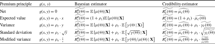
Table 3 summarizes the explicit forms of both estimators for several common premium principles, highlighting their structural coherence and the credibility estimator’s role as a natural extension of the Bayesian approach.
Bayesian and credibility estimators of variance-related risk premiums.

Table 3 Long description
Panel A: The table compares Bayesian and credibility estimators for different premium principles. Panel B: The premium principles include Net, Expected value, Variance, Standard deviation, and Modified variance. Panel C: For each premium principle, the table provides formulas for both Bayesian and credibility estimators. Panel D: The formulas involve variables such as rho, mu, gamma, and Theta, with specific operations like expectation and division.
The variance-related premium principle extends traditional actuarial pricing methodologies by incorporating not only the expected loss but also the associated uncertainty, typically represented by the variance. The estimators summarized in Table 3 offer a practical means of implementing this generalized principle. To demonstrate their application, we present a numerical example in which the latent risk variable follows a Gamma distribution, while the observed claim amounts are conditionally exponential given the risk parameter.
Example 4.1. Let
 $\Theta=\theta$
denote the underlying risk parameter, and assume that
 $X_{1},\ldots,X_{n}$
are conditionally i.i.d.
 $\mathrm{Exp}(\theta)$
with density
 \[f_{\theta}(x)=\theta e^{-\theta x}, \qquad x\gt0.\]
Hence,
 \[\mu(\Theta)=\mathbb{E}(X\mid\Theta)=\Theta^{-1},\qquad\gamma(\Theta)=\mathrm{Var}(X\mid\Theta)=\Theta^{-2}.\]
The prior distribution is taken as
 $\Theta\sim\Gamma(\alpha,\beta)$
with density
 \[\pi_{\Theta}(\theta)=\frac{\beta^{\alpha}}{\Gamma(\alpha)}\theta^{\alpha-1}e^{-\beta\theta},\qquad \theta\gt0,\ \alpha\gt4,\]
where
 $\alpha\gt4$
ensures the existence of the required higher-order moments. Under the Exponential-Gamma hierarchy, the marginal distribution of
 $X_i$
is
 \[f_{X_i}(x)=\alpha\beta^{\alpha}(x+\beta)^{-(\alpha+1)},\qquad x\gt0,\]
that is, a Pareto (Type II)/Lomax distribution (Lemonte and Cordeiro, Reference Lemonte and Cordeiro2013), exhibiting the heavy-tailed behavior induced by the mixing. Moreover,
 $\mu(\Theta)$
follows an inverse-gamma
 $(\alpha,\beta)$
distribution.
Given the sample
 $\mathbf{X}=(X_{1},\ldots,X_{n})$
with mean
 $\overline{X}_{n}$
, conjugacy implies
 \[[\Theta\mid\mathbf{X}]\sim\Gamma(\alpha+n,\beta+n\overline{X}_{n}),\]
so that the Bayesian estimators of the hypothetical mean and process variance are
 \[\mathbb{E}[\mu(\Theta)\mid\mathbf{X}]= \frac{\beta+n\overline{X}_{n}}{\alpha+n-1},\qquad\mathbb{E}[\gamma(\Theta)\mid\mathbf{X}]= \frac{(\beta+n\overline{X}_{n})^{2}} {(\alpha+n-1)(\alpha+n-2)}.\]
Consequently, all premium principles expressed in terms of
 $(\mu(\Theta),\gamma(\Theta))$
admit closed Bayesian forms. For example, the variance premium estimator is
 \[\widetilde{R_2^B(\Theta)}= \mathbb{E}[\mu(\Theta)\mid\mathbf{X}]+\rho_{2}\,\mathbb{E}[\gamma(\Theta)\mid\mathbf{X}].\]
The prior moments are given by
 \[\mu_0 = \frac{\beta}{\alpha-1}, \quad\tau^2 = \frac{\beta^2}{(\alpha-1)^2(\alpha-2)}, \quad\gamma_0 = \frac{\beta^2}{(\alpha-1)(\alpha-2)}, \quad\lambda = \frac{2\beta^4(2\alpha-5)}{(\alpha-1)^2(\alpha-2)^2(\alpha-3)(\alpha-4)}.\]
For exponential claims, the fourth conditional central moment leads to
 \[u_4(\Theta) = \frac{9}{\Theta^4}, \quad\delta_n(\Theta) = \frac{2(4n-3)}{\Theta^4 n(n-1)}, \quad\delta_n = \frac{2(4n-3)\,\beta^4}{n(n-1)(\alpha-1)(\alpha-2)(\alpha-3)(\alpha-4)}.\]
The associated credibility factors for the hypothetical mean and process variance are
 \begin{equation*}Z_{n}=\frac{n\tau ^{2}}{n\tau ^{2}+\gamma _{0}}=\frac{n}{n+\alpha -1},\text{}t_{n}^{\ast }=\frac{\lambda }{\lambda +\delta _{n}}=\frac{1}{1+\frac{(4n-3)}{n(n-1)}\cdot \frac{(\alpha -1)(\alpha -2)}{2\alpha -5}}.\end{equation*}
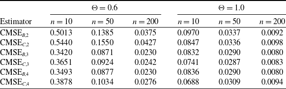
These expressions provide all quantities required to compute both the Bayesian and credibility estimators for the considered premium principles. Their accuracy can be assessed through the conditional mean squared error (CMSE),
 \[\mathrm{CMSE}_{k,i}\!\left[\widetilde{R_{i}^{k}(\Theta)}\right]=\mathbb{E}\!\left[\left(\widetilde{R_{i}^{k}(\Theta)}-R_{i}(\Theta)\right)^{2}\Big|\Theta\right],\]
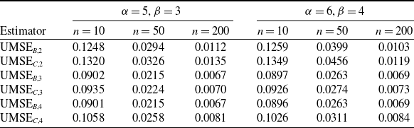
and the unconditional mean squared error (UMSE),
 \[\mathrm{UMSE}_{k,i}\!\left[\widetilde{R_{i}^{k}(\Theta)}\right]=\mathbb{E}\!\left[\left(\widetilde{R_{i}^{k}(\Theta)}-R_{i}(\Theta)\right)^{2}\right],\]
where
 $k=B$
or C and
 $i=0,1,2,3,4$
correspond to the net, expected value, variance, standard deviation, and modified variance premium principles.
For the parameter choices
 $\alpha=6$
,
 $\beta=4$
,
 $\rho_{1}=\rho_{2}=0.2$
, and
 $\rho_{3}=\rho_{4}=0.3$
, Monte Carlo simulations in R are conducted to compute the conditional mean squared errors (conditional MSEs, CMSEs) for risk levels
 $\Theta=0.6$
and
 $\Theta=1.0$
across sample sizes
 $n=10,50,200$
. The resulting conditional MSEs are reported in Table 4.Footnote
1
Here, we only display the results for
 $i=2,3,4$
because the premiums for
 $i=0$
and
 $i=1$
coincide under both Bayesian and credibility approaches and including them would be redundant.
Conditional MSEs of Bayesian and credibility estimators.

Table 4 Long description
A table comparing conditional mean squared errors (CMSEs) of Bayesian and credibility estimators for different sample sizes and risk levels. The table has 6 columns and 6 rows, including headers. The columns are labeled with risk levels (Theta = 0.6 and Theta = 1.0) and sample sizes (n = 10, n = 50, n = 200). The rows are labeled with different estimators (CMSE_B,2, CMSE_C,2, CMSE_B,3, CMSE_C,3, CMSE_B,4, CMSE_C,4). Each cell contains a numerical value representing the CMSE for the corresponding estimator, sample size, and risk level. The values decrease as the sample size increases, indicating that the errors decline substantially with larger sample sizes. The errors are consistently smaller for larger values of Theta, reflecting higher precision for less volatile risks. The Bayesian and credibility estimators exhibit almost identical performance for large sample sizes, but the Bayesian estimator generally achieves slightly lower mean squared errors for small sample sizes.
Furthermore, to evaluate the unconditional mean squared errors (unconditional MSEs, UMSEs), values of
 $\Theta$
are randomly generated from the Gamma prior. Two different parameter settings
 $(\alpha,\beta)$
are considered, and numerical simulations are conducted to compute the unconditional MSEs for each credibility estimator under the various premium principles. The resulting unconditional MSEs are reported in Table 5.
Unconditional MSEs of Bayesian and credibility estimators.

Table 5 Long description
A table comparing unconditional mean squared errors of Bayesian and credibility estimators for different sample sizes and parameter settings. The table has six columns and six rows, including headers. The columns are labeled with different sample sizes (n = 10, n = 50, n = 200) for two parameter settings (alpha = 5, beta = 3 and alpha = 6, beta = 4). The rows are labeled with different estimators (UMSE_B_2, UMSE_C_2, UMSE_B_3, UMSE_C_3, UMSE_B_4, UMSE_C_4). Each cell contains a numerical value representing the unconditional mean squared error for the corresponding estimator and sample size. The values decrease as the sample size increases, indicating that the errors decline substantially with larger sample sizes. The table provides a detailed comparison of the performance of Bayesian and credibility estimators under different conditions.
From Tables 4 to 5, it is evident that both conditional MSEs and unconditional MSEs decline substantially as the sample size n increases. The errors are consistently smaller for larger values of
 $\Theta$
, reflecting the higher precision attainable for less volatile risks. Moreover, while the Bayesian and credibility estimators exhibit almost identical performance for large sample sizes, the Bayesian estimator generally achieves slightly lower mean squared errors when the sample size is small.
Finally, we examine the asymptotic behavior of the credibility estimator
 $\widetilde{R_{i}^{C}(\Theta)}$
for
 $\alpha=6$
,
 $\beta=4$
,
 $\rho_{1}=\rho_{2}=0.2$
,
 $\rho_{3}=\rho_{4}=0.3$
, and
 $\Theta=1.4$
. Figure 3 presents kernel density estimates of
 $\widetilde{R_{i}^{C}(\Theta)}$
for sample sizes
 $n=5$
and
 $n=50$
, with dashed lines indicating the theoretical premium values. As the sample size increases from
 $n=5$
to
 $n=50$
, the empirical distributions become more symmetric and more concentrated around the theoretical values, providing clear numerical evidence in favor of the estimator’s asymptotic normality.
Kernel density estimates of credibility estimators for different sample sizes.

Under this hierarchical specification, the marginal distribution of
 $X_i$
follows a Pareto (Type II) or Lomax distribution, which naturally arises from the exponential–gamma conjugate structure. Furthermore, since
 $\mu(\Theta) = 1/\Theta$
, the transformed random variable
 $\mu(\Theta)$
follows an inverse Gamma distribution with parameters
 $(\alpha, \beta)$
(Klugman et al., Reference Klugman, Panjer and Willmot2019). This alternative representation provides valuable insight into the mean–variance relationship inherent in the exponential–gamma model.
4.2 Practical applications
To illustrate the implementation of the proposed credibility framework, we use the dataset fremotor2freq9907u
Footnote
2
available in the CASdatasets package in R (Rizzo, Reference Rizzo2019; Dutang and Charpentier, Reference Dutang and Charpentier2024). Each policy is treated as a separate credibility unit associated with a latent risk parameter
 $\Theta_i$
(
 $i=1,\ldots,K$
). Conditional on
 $\Theta_i$
, the observed annual claim counts
 $\{X_{ij}\}_{j=1}^{n_i}$
are assumed i.i.d. with conditional distribution
 $f_{\theta_i}(x)$
. Additional implementation details, including data processing, structural parameter estimation, and bootstrap approximation of
 $\delta_{n_i}$
and
 $\lambda$
, are provided in Appendix A.6.
Based on the sample, we estimate the five structural parameters required for the credibility model, namely
 $\mu_{0}$
,
 $\gamma_{0}$
,
 $\tau^{2}$
,
 $\delta_{n_{i}}$
, and
 $\lambda$
. Following Bühlmann and Gisler (Reference Bühlmann and Gisler2005, p. 94),
 $\mu_{0}$
is the portfolio-level mean,
 $\gamma_{0}$
is the within-policy variance, and
 $\tau^{2}$
is the between-policy variance.
The resulting unbiased estimates of the structural parameters are summarized in Table 6. The policy-specific dispersion parameters
 $\widehat{\delta}_{n_i}$
can be obtained from these estimates as described in Appendix A.6, but are not listed here for brevity.
Given the estimates in Table 6, we next compute credibility estimates of risk premiums using the sample. At this stage, the structural parameters are treated as known, and the resulting credibility estimators correspond to empirical Bayes estimators in the sense of Robbins (Reference Robbins1964), with actuarial developments discussed in Mashayekhi (Reference Mashayekhi2002).
Structural parameter estimates.

Table 6 Long description
A table with two rows and five columns. The first row contains the headers: Parameter and Estimate. The second row lists the parameters and their corresponding estimates: gamma sub 0, 0.1680; tau squared, 0.0585; delta, 0.2345; lambda, 0.1801; mu sub 0, 0.1635.
Before calculating premiums, we determine the safety loading coefficients
 $\rho_i$
(
 $i = 1, \ldots, 4$
), which link risk-based estimates to actual premium levels under different principles. Following Yong et al. (Reference Yong, Zeng and Zhang2025), these coefficients are calibrated via a value-at-risk (VaR) approach at confidence level
 $p = 0.9$
. Let Y denote the aggregate claim amount. The loadings are defined by

where
 $\mathbb{E}[Y]$
,
 $\mathrm{Var}(Y)$
, and
 $\mathrm{VaR}_{p}(Y)$
are estimated using, respectively, the sample mean
 $\overline{X}_{i}$
, the sample variance
 $\widetilde{S}_{n_i}^{2}$
, and the empirical p-quantile of policy i computed from the sample (
 $i = 1,2,\ldots,K$
). This VaR-based calibration ensures that, under each premium principle, the premiums cover aggregate claims at the specified confidence level.
Using the estimated structural parameters and calibrated safety loadings
 $\rho_i$
, we then compute the credibility estimator in (4.1) under the net, expected value, variance, standard deviation, and modified variance principles. The sample still contains a large number of policies, so it is not feasible to report results for all contracts. For illustration, we select seven policies from the sample and report their credibility-adjusted premium estimates in Table 7.
Estimated premiums for seven sampled policies under different premium principles.

Table 7 Long description
A table with seven rows and six columns comparing estimated premiums for seven sampled policies under different premium principles. The columns are labeled with Policy IDs: PN148469, PN191262, PN105635, PN62080, PN76584, PN38328, and PN6536. The rows are labeled with different premium principles: Net premium principle, Expected value, Variance principle, Standard deviation, and Modified variance. Each cell contains a numerical value representing the estimated premium under the respective principle. Row 1: Net premium principle, 0.7122, 0.4206, 0.2139, 0.1867, 0.1656, 0.2502, 0.1352. Row 2: Expected value, 2.1774, 1.2859, 0.6538, 0.5708, 0.5064, 0.7648, 0.4133. Row 3: Variance principle, 2.0351, 1.4360, 1.0377, 0.8798, 0.7639, 1.0642, 0.6048. Row 4: Standard deviation, 1.3793, 1.0051, 0.7404, 0.6696, 0.6143, 0.7735, 0.5327. Row 5: Modified variance, 1.0160, 0.8154, 0.8439, 0.7939, 0.7563, 0.7823, 0.7033.
Table 7 shows the resulting premiums under the different principles. As expected, the net premium corresponds to the pure risk expectation, while the other principles incorporate additional loadings through the parameters
 $\rho_i$
. The variance and modified variance principles produce higher premiums for policies with more volatile claim experience, reflecting their sensitivity to underlying risk heterogeneity and the ability of the credibility-adjusted framework to differentiate premiums accordingly.
5. Concluding remarks
This paper develops a novel framework for estimating process variance, extending the classical Bühlmann credibility theory. Unlike traditional approaches that focus primarily on the hypothetical mean, the proposed method directly addresses the variability of the underlying risk process, capturing higher-order moments and portfolio heterogeneity. This enables the derivation of explicit credibility-adjusted risk premiums under multiple premium principles, including net premium, expected value, variance, standard deviation, and modified variance principles.
By embedding credibility theory within a Bayesian framework, we address some of the limitations associated with conventional Bayesian risk premium estimation. The methodology seamlessly integrates observed claim experience with the underlying portfolio risk structure, producing premiums that reflect both individual policy history and collective characteristics. Calibration of safety loading factors in a data-driven manner ensures that the resulting premiums are consistent with solvency requirements and responsive to varying levels of risk exposure.
The proposed approach is practical, computationally tractable, and operates under mild assumptions without requiring full specification of population or prior distributions. Rigorous theoretical analysis confirms that the estimators possess desirable statistical properties, while empirical results based on real insurance data demonstrate their robustness and practical relevance. The framework effectively differentiates premiums according to policy-specific risk profiles and premium principles, supporting more accurate and informed pricing decisions.
Looking forward, the methodology can be extended to multidimensional risk settings, incorporate hierarchical or nonparametric priors for greater flexibility, and be combined with modern machine learning techniques to improve both estimation accuracy and computational efficiency. Applications beyond traditional insurance pricing, such as portfolio optimization or systemic risk assessment, may also benefit from this framework, illustrating its broad practical relevance.
Supplementary material
The supplementary material for this article can be found at https://doi.org/10.1017/asb.2026.10094.
Acknowledgements
The authors would like to express their sincere gratitude to the anonymous reviewers for their insightful comments and constructive suggestions. Their careful reading and valuable feedback have greatly enhanced the rigor, clarity, and overall quality of this manuscript. The authors also acknowledge the financial support from the National Social Science Fund of China under the Later Stage Project (Grant No. 25FTJB002).
Competing interests
No potential competing interest was reported by the authors.
Appendix A
A.1 The Proof of Theorem 2.1
Proof. For notational convenience, let
 \[\Phi = \mathbb{E}\Big[\big(R(\Theta) - b_0 - \sum_{i=1}^{n} b_i X_i\big)^2\Big].\]
Since
 $X_1, \ldots, X_n$
are conditionally independent and identically distributed given
 $\Theta$
(i.e., conditionally exchangeable), all coefficients
 $b_i$
can be taken equal. This simplifies the original minimization problem from
 $n+1$
variables to just two:
 \[b_1 = b_2 = \cdots = b_n, \quad \text{and} \quad\min_{b_0,b_1} \mathbb{E}\Big[\big(R(\Theta) - b_0 - b_1 \sum_{i=1}^{n} X_i\big)^2\Big]= \min_{b_0,b_1} \mathbb{E}\Big[\big(R(\Theta) - b_0 - n b_1 \overline{X}_n\big)^2\Big],\]
where
 $\overline{X}_n = \frac{1}{n} \sum_{i=1}^{n} X_i$
.
Taking the derivative of
 $\Phi$
with respect to
 $b_0$
and setting it to zero yields the optimal intercept:
 \[b_0 = \mathbb{E}[R(\Theta)] - n b_1 \mathbb{E}[X_i] = R_0 - n b_1 \mu_0.\]
Substituting this expression back into
 $\Phi$
and differentiating with respect to
 $b_1$
, we obtain
 \[\frac{\partial \Phi}{\partial b_1} = n \,\mathrm{Cov}(R(\Theta), X_i) - n^2 b_1 \,\mathrm{Var}(X_i) - n(n-1) b_1 \,\mathrm{Cov}(X_i, X_j) = 0, \quad i \neq j.\]
Here, we use the standard Bühlmann variance decomposition, which separates the variance into individual and common components:
 \[\mathrm{Var}(X_i) = \sigma^2 + \tau^2, \quad\mathrm{Cov}(X_i, X_j) = \tau^2, \quad\mathrm{Cov}(R(\Theta), X_i) = \varphi.\]
Solving for
 $b_1$
gives
 \[\widehat{b}_1 = \frac{\varphi}{\sigma^2 + n \tau^2}.\]
Finally, we have
 \[\widehat{R_C(\Theta)} = \widehat{b}_0 + n \widehat{b}_1 \overline{X}_n= R_0 - n \widehat{b}_1 \mu_0 + n \widehat{b}_1 \overline{X}_n= T_n \overline{X}_n + \left(1 - \frac{T_n \mu_0}{R_0}\right) R_0.\]
This completes the proof.
A.2 The Proof of Theorem 2.2
Proof. We first prove the sufficiency part. Suppose there exist constants s and
 $t$
such that
 $g\left( \gamma(\Theta)\right) =s\mu(\Theta)+t$
, then we have
 \[R(\Theta)=\mu(\Theta)+\rho\cdot g(\gamma(\Theta))=\mu(\Theta)+\rho(s\mu(\Theta)+t)=(1+\rho s)\mu(\Theta)+\rho t.\]
Thus, we have
 $R_{0}=(1+\rho s)\mu_{0}+\rho t$
,
 $\varphi=(1+\rho s)\tau^{2}$
, and
 \[T_{n}=\frac{(1+\rho s)n\tau^{2}}{n\tau^{2}+\sigma^{2}}=(1+\rho s)Z_{n},\]
where
 $Z_{n}$
is given by (2.3). The credibility estimation of
 $R_{C}(\Theta)$
is simplified to
 \[\widehat{R_C(\Theta)}=T_{n}\overline{X}_n+R_{0}-T_{n}\mu_{0}=(1+\rho s)Z_{n}\overline{X}_n+(1+\rho s)\mu_{0}(1-Z_{n})+\rho t.\]
By the Strong Law of Large Numbers, we have
 $\overline{X}_n\rightarrow\mu(\Theta)$
almost surely as
 $n\rightarrow\infty$
. Given that
 $Z_{n}\rightarrow1$
and
 $1-Z_{n}\rightarrow0$
, the strong consistency for
 $\widehat{R_C(\Theta)}$
is given by
 \[\widehat{R_C(\Theta)}\rightarrow(1+\rho s)\mu(\Theta)+\rho t=R(\Theta).\]
Next, we prove the necessity part. Suppose
 $\widehat{R_C(\Theta)}$
is consistent with respect to
 $R(\Theta)$
. We denote
 $\mathrm{Cov}\left(\mu(\Theta), g\left( \gamma(\Theta)\right) \right) = \eta$
and
 $\mathbb{E}\left[ g\left( \gamma(\Theta)\right) \right] = \lambda$
for convenience. Due to
 $R_{0} = \mathbb{E}\left[ R(\Theta) \right] = \mu_{0} +\lambda$
and
 \[\varphi= \mathrm{Cov}\left( R(\Theta), R(\Theta) \right) = \mathrm{Cov}\left( \mu(\Theta) + g\left( \gamma(\Theta)\right) , \mu(\Theta)\right) =\tau^{2} + \eta,\]
we have
 \[T_{n} = \frac{n\varphi}{n\tau^{2}+\sigma^{2}} = \frac{\varphi}{\tau^{2}+\sigma^{2}/n} \rightarrow1 + \frac{\eta}{\tau^{2}}.\]
Therefore, we have
 \begin{align*}\widehat{R_C(\Theta)} & \rightarrow\left( 1 + \frac{\eta}{\tau^{2}}\right) \mu(\Theta) + \mu_{0} + \lambda- \left( 1 + \frac{\eta}{\tau^{2}}\right) \mu_{0}\\[5pt] & = \left( 1 + \frac{\eta}{\tau^{2}} \right) \mu(\Theta) + \lambda-\frac{\eta}{\tau^{2}} \mu_{0}\\[5pt] & = s\mu(\Theta) + t,\end{align*}
where
 $s = \left( 1 + \frac{\eta}{\tau^{2}} \right) $
and
 $t = \lambda-\frac{\eta}{\tau^{2}} \mu_{0}$
are constants. This completes the proof.
A.3 The Proof of Theorem 3.1
Proof. Note that as
 $n\rightarrow\infty$
,
 $w_{n}^{\ast}=\frac{n\lambda}{n\lambda+v}\rightarrow1$
. From the strong law of large numbers, we have
 $S_{n}^{2}\rightarrow\mathbb{E}\left( Y_{1}|\Theta\right) =\gamma(\Theta)$
, almost surely (a.s.). Thus, it follows that:
 \[\widehat{\gamma_C(\Theta)}=w_{n}^{\ast}\cdot S_{n}^{2}+\left( 1-w_{n}^{\ast}\right) \gamma_{0}\rightarrow\gamma(\Theta), a.s..\]
Additionally, from the central limit theorem, we have
 \[\sqrt{n}(S_{n}^{2} - \gamma(\Theta)) \overset{d}{\rightarrow} \mathcal{N}(0,\sigma_{\gamma}^{2}(\Theta)).\]
On the other hand, we obtain that
 \[\sqrt{n}\left[ \widehat{\gamma_C(\Theta)}-\gamma(\Theta)\right] -\sqrt{n}(S_{n}^{2}-\gamma(\Theta))=\sqrt{n}\left( 1-w_{n}^{\ast}\right) \left(\gamma_{0}-S_{n}^{2}\right) =O_{p}\left( \frac{1}{\sqrt{n}}\right)\overset{\mathbb{P}}{\longrightarrow}0,\]
which implies, according to Slutsky’s Theorem (Kapadia et al., Reference Kapadia, Chan and Moyé2017), that:
 \[\sqrt{n}\left[ \widehat{\gamma_C(\Theta)}-\gamma(\Theta)\right] \overset{d}{\rightarrow}\mathcal{N}(0,\sigma_{\gamma}^{2}(\Theta)).\]
This completes the proof.
A.4 The Proof of Theorem 3.2
Proof. According to the exchangeability of variables for
 $Y_{i}=(X_{i}-\overline{X})^{2}$
,
 $i=1,2,\ldots,n$
, the minimization problem (3.2) is equivalent to A
 \begin{equation}\min_{a_{0},b\in\mathbb{R}}\mathbb{E}\Big[ \big( \gamma(\Theta)-a_{0}-b{\tilde{S}_n^{2}}\big) ^{2}\Big] ,\end{equation}
where
 $b=\left( n-1\right) a_{1}=\cdots=\left( n-1\right) a_{n}$
. From the standard Lagrange methods, the optimal selection of
 $a_{0}$
and b are the solutions of the following normal equations:
 \begin{equation}\left\{\begin{array}[c]{c}\mathbb{E}\big[ \gamma(\Theta)\big] =a_{0}+b\mathbb{E}\big[{\tilde{S}_n^{2}}\big] \\[5pt] \mathrm{Cov}\big( \gamma(\Theta),{\tilde{S}_n^{2}}\big) =b\mathrm{Var}\big({\tilde{S}_n^{2}}\big)\end{array}\right. . \end{equation}
In Appendix 1, we have demonstrated the following conclusions:
 \[\mathbb{E}\big( {\tilde{S}_n^{2}}\mid\Theta\big) =\gamma(\Theta)\quad\text{and}\quad\mathrm{Var}\big( {\tilde{S}_n^{2}}\mid\Theta\big) =\delta_{n}(\Theta),\]
thus we have
 \[\mathbb{E}\big[ \gamma(\Theta)\big] =\mathbb{E}\big[ {\tilde{S}_n^{2}}\big]=\gamma_{0},\quad\mathrm{Var}\big( {\tilde{S}_n^{2}}\big) =\delta_{n}+\lambda,\quad\mathrm{Cov}\big( \gamma(\Theta),{\tilde{S}_n^{2}}\big) =\lambda.\]
By solving the Equation (A2), the solutions for
 $a_{0}$
and b are given by
 \[\widehat{a_{0}}=\left( 1-\widehat{b}\right) \gamma_{0},\quad\widehat{b}=\frac{\lambda}{\delta_{n}+\lambda}.\]
Thus, it follows that
 \begin{equation}\widetilde{\gamma_C(\Theta)}=\widehat{a_{0}}+\widehat{b}{\tilde{S}_n^{2}}=t_{n}^{\ast}\cdot{\tilde{S}_n^{2}}+\left( 1-t_{n}^{\ast}\right) \gamma_{0}.\end{equation}
A.5 The Proof of Theorem 3.3
Proof. When the mean is unknown, the sample variance can be written as
 \begin{equation*}{\tilde{S}_{n}^{2}} = \frac{n}{n-1}\left[ \frac{1}{n}\sum_{i=1}^{n}X_{i}^{2} - \overline{X}_{n}^{2} \right],\end{equation*}
where
 $\overline{X}_{n} = \frac{1}{n}\sum_{i=1}^{n}X_{i}$
denotes the sample mean. By the strong law of large numbers, conditional on
 $\Theta$
, we almost surely have
 \begin{equation*}\frac{1}{n}\sum_{i=1}^{n}X_{i} \longrightarrow \mu(\Theta),\qquad\frac{1}{n}\sum_{i=1}^{n}X_{i}^{2} \longrightarrow \mathbb{E}\!\left[X_{1}^{2}\mid\Theta\right],\end{equation*}
as
 $n\to\infty$
. This immediately yields
 \begin{equation*}{\tilde{S}_{n}^{2}} \longrightarrow \gamma(\Theta) \qquad \text{almost surely}.\end{equation*}
The credibility estimator is given by
 \begin{equation*}\widetilde{\gamma_{C}(\Theta)} = t_{n}^{\ast}\,{\tilde{S}_{n}^{2}} + (1-t_{n}^{\ast})\,\gamma_{0},\end{equation*}
and the fact that
 $t_{n}^{\ast}\to 1$
implies
 \begin{equation*}\widetilde{\gamma_{C}(\Theta)} \longrightarrow \gamma(\Theta) \qquad \text{almost surely}.\end{equation*}
To examine the Bayesian estimator, note that
 \[\widetilde{\gamma_{B}(\Theta)} = \mathbb{E}\!\left[\gamma(\Theta)\,\middle|\,X_{1},\ldots,X_{n}\right],\]
which, as a conditional expectation, minimizes the mean squared error among all
 $\mathcal{F}_{n}$
-measurable estimators. Therefore,
 \begin{equation*}0 \leq\mathbb{E}\!\left[\left(\widetilde{\gamma_{B}(\Theta)}-\gamma(\Theta)\right)^{2}\right]\leq\mathbb{E}\!\left[\left(\widetilde{\gamma_{C}(\Theta)}-\gamma(\Theta)\right)^{2}\right] = \frac{\delta_{n}\lambda}{\delta_{n}+\lambda} \longrightarrow 0,\end{equation*}
which shows that
 $\widetilde{\gamma_{B}(\Theta)}$
converges to
 $\gamma(\Theta)$
in mean square.
Moreover, since
 $\widetilde{\gamma_{B}(\Theta)}$
forms a martingale with respect to
 $\mathcal{F}_{n}=\sigma(X_{1},\ldots,X_{n})$
, the martingale convergence theorem (Schmidt, Reference Schmidt1990) guarantees almost sure convergence:
 \[\widetilde{\gamma_{B}(\Theta)} \overset{a.s.}{\longrightarrow} \gamma(\Theta).\]
To derive the asymptotic normality of the credibility estimator, define
 $W_{i}=(X_{i}-\mu(\Theta))^{2}$
and
 \[\overline{W}=\frac{1}{n}\sum_{i=1}^{n}W_{i}.\]
Conditional on
 $\Theta$
, we have
 \[\mathbb{E}[W_{i}\mid\Theta]=\gamma(\Theta),\qquad\mathrm{Var}(W_{i}\mid\Theta) = u_{4}(\Theta)-\gamma^{2}(\Theta) = \sigma_{\upsilon}^{2}(\Theta),\]
and the classical central limit theorem gives
 \begin{equation*}\sqrt{n}\big(\overline{W}-\gamma(\Theta)\big) \overset{d}{\longrightarrow} \mathcal{N}\!\left(0,\sigma_{\upsilon}^{2}(\Theta)\right).\end{equation*}
In addition,
 \[{\tilde{S}_{n}^{2}} = \overline{W} - \big(\overline{X}_{n}-\mu(\Theta)\big)^{2} + O\!\left(\frac{1}{n}\right),\]
and using
 $\overline{X}_{n}-\mu(\Theta)=O(n^{-1/2})$
, we obtain
 \[\sqrt{n}\!\left[{\tilde{S}_{n}^{2}}-\gamma(\Theta)\right] - \sqrt{n}\!\left[\overline{W}-\gamma(\Theta)\right] \longrightarrow 0 \qquad \text{in probability}.\]
Thus, by Slutsky’s theorem,
 \begin{equation*}\sqrt{n}\big({\tilde{S}_{n}^{2}}-\gamma(\Theta)\big) \overset{d}{\longrightarrow} \mathcal{N}\!\left(0,\sigma_{\upsilon}^{2}(\Theta)\right).\end{equation*}
Finally,
 \[\sqrt{n}\big(\widetilde{\gamma_{C}(\Theta)}-\gamma(\Theta)\big) = \sqrt{n}\big({\tilde{S}_{n}^{2}}-\gamma(\Theta)\big) + \sqrt{n}(1-t_{n}^{\ast}) \big(\gamma_{0}-{\tilde{S}_{n}^{2}}\big),\]
and the second term is
 $o_{p}(1)$
because
 $(1-t_{n}^{\ast})=O(n^{-1})$
. Therefore,
 \begin{equation*}\sqrt{n}\big(\widetilde{\gamma_{C}(\Theta)}-\gamma(\Theta)\big) \overset{d}{\longrightarrow} \mathcal{N}\!\left(0,\sigma_{\upsilon}^{2}(\Theta)\right).\end{equation*}
Combining the above results, we conclude that when the mean is unknown, both the credibility and Bayesian estimators are strongly consistent, and in addition, the credibility estimator is asymptotically normal.
A.6 Empirical implementation and structural parameter estimation
This appendix provides a comprehensive description of the empirical implementation underlying the practical application in Section 4.2. The presentation follows the chronological order of the empirical procedure, beginning with data preparation, followed by structural parameter estimation, bootstrap approximation of dispersion quantities, and concluding with premium computation.
The empirical analysis is based on the dataset fremotor2freq9907u from the CASdatasets package in R. For each policy, we retain the policy identifier IDpol and the annual claim-count variables
 \[\texttt{NbClaim1999}, \texttt{NbClaim2000}, \ldots, \texttt{NbClaim2006}.\]
The available annual claim counts for each policy i are arranged as a longitudinal claim history
 $\{X_{ij}\}_{j=1}^{n_i}$
, where
 $n_i$
denotes the number of non-missing annual observations. Policies with fewer than two observed years are excluded, ensuring that
 $(n_i-1) \neq 0$
for the estimation of within-policy variance. Each policy is treated as a single credibility unit associated with an unobserved risk parameter
 $\Theta_i$
. The analysis is conducted directly on annual claim counts without constructing exposure-adjusted frequencies.
Based on the sample, the structural parameters are computed as follows. Let K denote the number of policies in the sample and
 $N=\sum_{i=1}^{K} n_i$
the total number of observations. The structural mean and within-policy variance are estimated by the unbiased formulas
 \begin{equation*}\widehat{\mu}_{0} = \frac{1}{N} \sum_{i=1}^{K} n_i \overline{X}_{n_i},\qquad\widehat{\gamma}_0 = \frac{1}{\sum_{i=1}^{K} (n_i-1)} \sum_{i=1}^{K} \sum_{j=1}^{n_i} (X_{ij} - \overline{X}_{n_i})^2,\end{equation*}
where
 $\overline{X}_{n_i} = \frac{1}{n_i} \sum_{j=1}^{n_i} X_{ij}$
is the mean claim count for policy i. The between-policy variance is estimated as
 \begin{equation*}\widehat{\tau}^2 = \frac{N}{N^2 - \sum_{i=1}^{K} n_i^2}\left[ \sum_{i=1}^{K} n_i (\overline{X}_{n_i} - \overline{\overline{X}})^2 - (K-1)\widehat{\gamma}_0 \right],\end{equation*}
with
 $\overline{\overline{X}} = \frac{1}{N}\sum_{i=1}^{K} n_i \overline{X}_{n_i}$
being the overall mean.
The variance-based credibility estimator additionally requires the dispersion quantities
 \begin{equation*}\delta_{n_i} = \mathbb{E}[\mathrm{Var}(\tilde{S}_{n_i}^2 \mid \Theta_i)],\qquad\lambda = \mathrm{Var}[\gamma(\Theta_i)],\end{equation*}
where
 $\tilde{S}_{n_i}^2 = \frac{1}{n_i-1} \sum_{j=1}^{n_i} (X_{ij}-\overline{X}_{n_i})^2$
and
 $\gamma(\Theta_i) = \mathrm{Var}(X_{ij} \mid \Theta_i)$
. Since closed-form estimators for
 $\delta$
and
 $\lambda$
are generally unavailable, these quantities are approximated via a nonparametric bootstrap applied independently within each policy. Specifically, for
 $m=10{,}000$
bootstrap replications, bootstrap samples
 $\{ X_{ij}^{(t)} : i=1,\ldots,K;\ j=1,\ldots,n_i \},\ t=1,\ldots,m$
are generated. For each replication, the within-policy variance is computed as
 \begin{equation*}S_{i(t)}^2 = \frac{1}{n_i-1} \sum_{j=1}^{n_i} (X_{ij}^{(t)} - \overline{X}_{n_i}^{(t)})^2,\qquad\overline{X}_{n_i}^{(t)} = \frac{1}{n_i} \sum_{j=1}^{n_i} X_{ij}^{(t)}.\end{equation*}
The overall estimates of
 $\delta$
and
 $\lambda$
are then obtained by
 \begin{equation*}\widehat{\delta} = \frac{1}{K(m-1)} \sum_{i=1}^{K} \sum_{t=1}^{m} n_i (S_{i(t)}^2 - \overline{S_i^2})^2,\qquad\widehat{\lambda} = \frac{1}{m(K-1)} \sum_{i=1}^{K} \sum_{t=1}^{m} (S_{i(t)}^2 - \overline{S_t^2})^2,\end{equation*}
where
 $\overline{S_i^2} = \frac{1}{m}\sum_{t=1}^{m} S_{i(t)}^2$
and
 $\overline{S_t^2} = \frac{1}{K} \sum_{i=1}^{K} S_{i(t)}^2$
. The policy-specific dispersion parameters are then defined as
 $\widehat{\delta}_{n_i} = \widehat{\delta}/n_i$
for
 $i=1,\ldots,K$
.
Finally, premium estimates are computed using the estimated structural parameters and corresponding credibility factors. For illustration, Table 7 reports premiums for seven policies selected from the sample. Each reported policy corresponds to a single credibility unit, and the premiums incorporate the calibrated loading coefficients
 $\rho_i$
as described in Section 4.2.


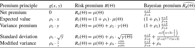
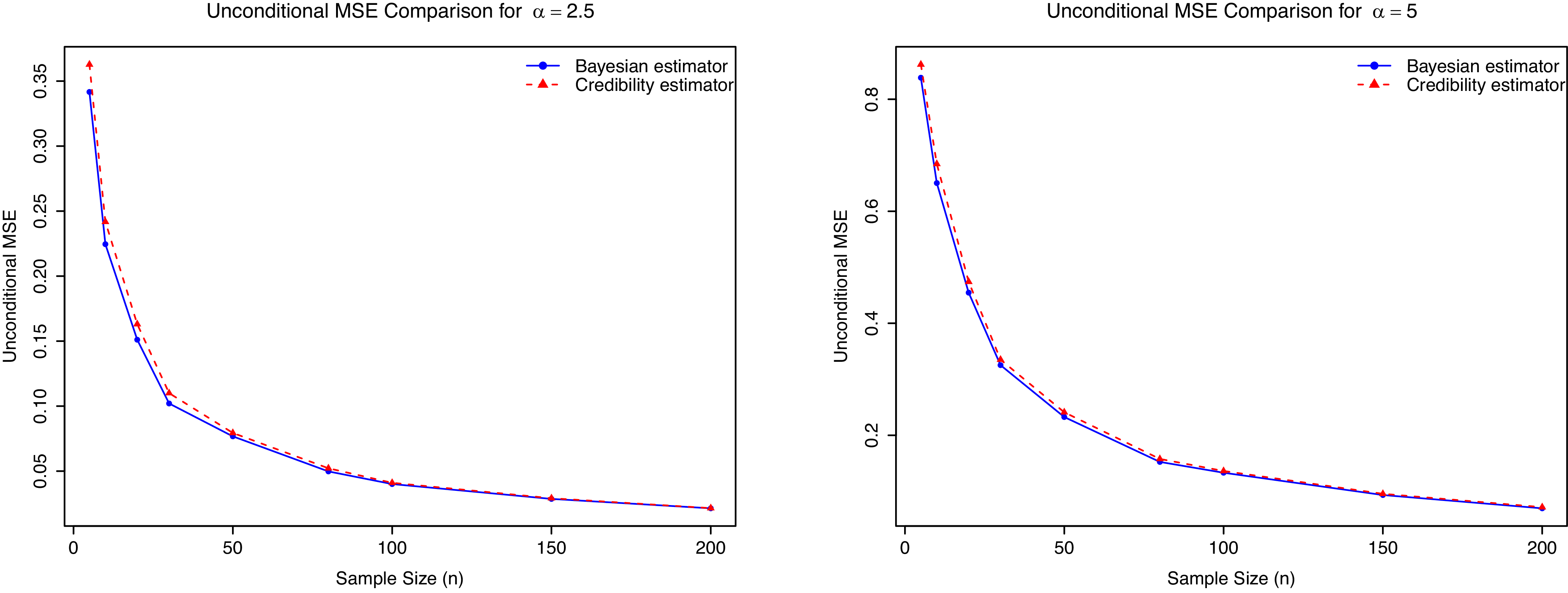
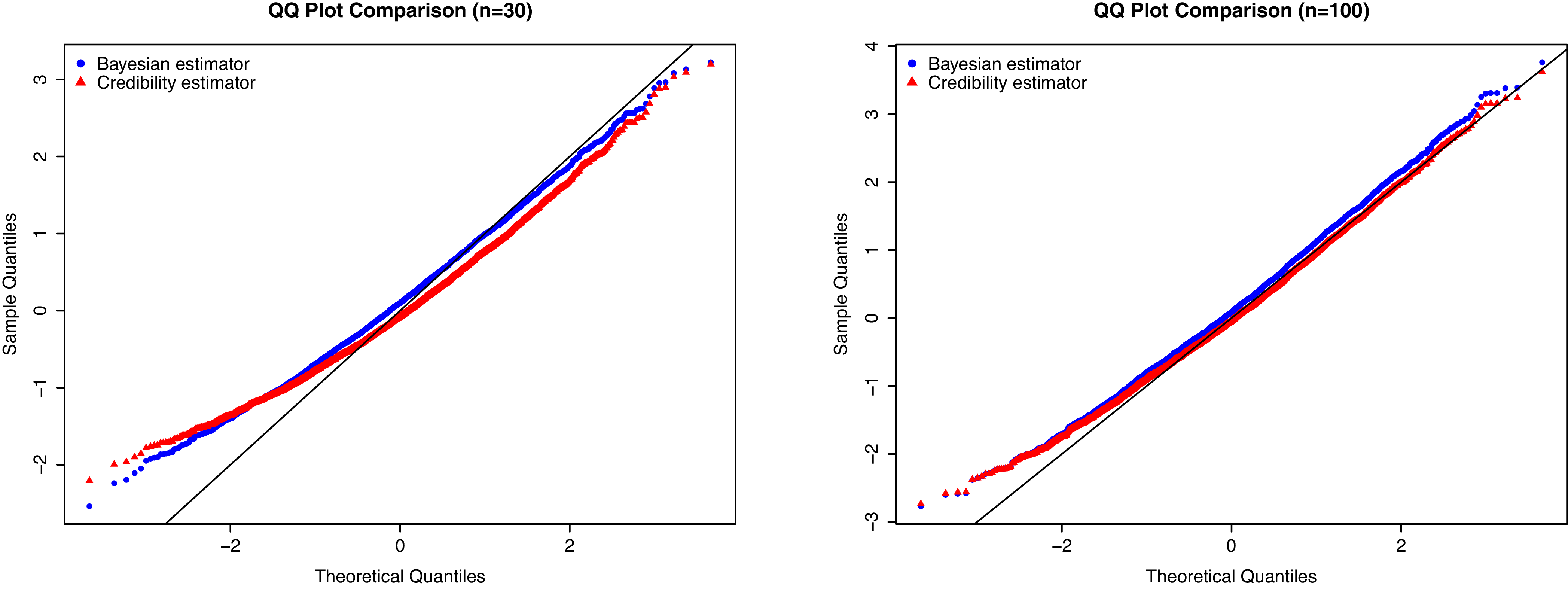
 Θ=1.5
 n=30
 n=100
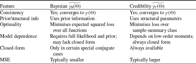
 γ(Θ)