1 Introduction
This survey article presents an overview of the fundamentals of direct methods for sparse matrix problems, from theory to algorithms and data structures to working pseudocode. It gives an in-depth presentation of the many algorithms and software available for solving sparse matrix problems, both sequential and parallel. The focus is on direct methods for solving systems of linear equations, including LU, QR, Cholesky, and other factorizations, forward/backsolve, and related matrix operations. Iterative methods, solvers for eigenvalue and singular-value problems, and sparse optimization problems are beyond the scope of this article.
1.1 Outline
∙ In Section 1.2, below, we first provide a list of books and prior survey articles that the reader may consult to further explore this topic.
∙ Section 2 presents a few basic data structures and some basic algorithms that operate on them: transpose, matrix–vector and matrix–matrix multiply, and permutations. These are often necessary for the reader to understand and perhaps implement, to provide matrices as input to a package for solving sparse linear systems.
∙ Section 3 describes the sparse triangular solve, with both sparse and dense right-hand sides. This kernel provides a useful background in understanding the non-zero pattern of a sparse matrix factorization, which is discussed in Section 4, and also forms the basis of the basic Cholesky and LU factorizations presented in Sections 5 and 6.
∙ Section 4 covers the symbolic analysis phase that occurs prior to numerical factorization: finding the elimination tree, the number of non-zeros in each row and column of the factors, and the non-zero patterns of the factors themselves (or their upper bounds in case numerical pivoting changes things later on). The focus is on Cholesky factorization but this discussion has implications for the other kinds of factorizations as well (
 $\text{LDL}^{\text{T}}$, LU, and QR).
∙ Section 5 presents the many variants of sparse Cholesky factorization for symmetric positive definite matrices, including early methods of historical interest (envelope and skyline methods), and up-looking, left-looking, and right-looking methods. Multifrontal and supernodal methods (for Cholesky, LU,
$\text{LDL}^{\text{T}}$ and QR) are presented later on.∙ Section 6 considers the LU factorization, where numerical pivoting becomes a concern. After describing how the symbolic analysis differs from the Cholesky case, this section covers left-looking and right-looking methods, and how numerical pivoting impacts these algorithms.
∙ Section 7 presents QR factorization and its symbolic analysis, for both row-oriented (Givens) and column-oriented (Householder) variants. We also consider alternative methods for solving sparse least-squares problems, based on augmented systems or on LU factorization.
∙ Section 8 is on the ordering problem, which is to find a good permutation for reducing fill-in, work, or memory usage. This is a difficult problem (it is NP-hard, to be precise). This section presents the many heuristics that have been created that attempt to find a decent solution to the problem. These heuristics are typically applied first, prior to the symbolic analysis and numeric factorization, but it appears out of order in this article, since understanding matrix factorizations (Sections 4–7) is a prerequisite in understanding how to best permute the matrix.
∙ Section 9 presents the supernodal method for Cholesky and LU factorization, in which adjacent columns in the factors with identical non-zero pattern (or nearly identical) are ‘glued’ together to form supernodes. Exploiting this common substructure greatly improves memory traffic and allows for computations to be done in dense submatrices, each representing a supernodal column.
∙ Section 10 discusses the frontal method, which is another way of organizing the factorization in a right-looking method, where a single dense submatrix holds the part of the sparse matrix actively being factorized, and rows and columns come and go during factorization. Historically, this method precedes both supernodal and multifrontal methods.
∙ Section 11 covers the many variants of the multifrontal method for Cholesky,
$\text{LDL}^{\text{T}}$, LU, and QR factorizations. In this method, the matrix is represented not by one frontal matrix but by many of them, all related to one another via the assembly tree (a variant of the elimination tree). As in the supernodal and frontal methods, dense matrix operations can be exploited within each dense frontal matrix.∙ Section 12 considers several topics that do not fit neatly into the above outline, yet which are critical to the domain of direct methods for sparse linear systems. Many of these topics are also active areas of research: update/downdate methods, parallel triangular solve, GPU acceleration, and low-rank approximations.
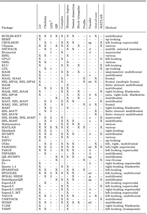
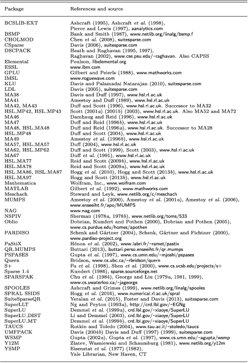
∙ Reliable peer-reviewed software has long been a hallmark of research in computational science, and in sparse direct methods in particular. Thus, no survey on sparse direct methods would thus be complete without a discussion of software, which we present in Section 13.


1.2 Resources
Sparse direct methods are a tightly coupled combination of techniques from numerical linear algebra, graph theory, graph algorithms, permutations, and other topics in discrete mathematics. We assume that the reader is familiar with the basics of this background. For further reading, Golub and Van Loan (Reference Golub and Van Loan2012) provide an in-depth coverage of numerical linear algebra and matrix computations for dense and structured matrices. Cormen, Leiserson and Rivest (Reference Cormen, Leiserson and Rivest1990) discuss algorithms and data structures and their analysis, including graph algorithms. MATLAB notation is used in this article (see Davis Reference Davis2011b for a tutorial).
Books dedicated to the topic of direct methods for sparse linear systems include those by Tewarson (1973), George and Liu (Reference George and Liu1981), Pissanetsky (Reference Pissanetsky1984), Duff, Erisman and Reid (Reference Duff, Erisman and Reid1986), Zlatev (Reference Zlatev1991), Björck (Reference Björck1996), and Davis (Reference Davis2006). Portions of Sections 2–8 of this article are condensed from Davis’s (Reference Davis2006) book. Demmel (Reference Demmel1997) interleaves a discussion of numerical linear algebra with a description of related software for sparse and dense problems. Chapter 6 of Dongarra, Duff, Sorensen and Van der Vorst (Reference Dongarra, Duff, Sorensen and Van der Vorst1998) provides an overview of direct methods for sparse linear systems. Several of the early conference proceedings in the 1970s and 1980s on sparse matrix problems and algorithms have been published in book form, including Reid (Reference Reid1971), Rose and Willoughby (1972), Duff (Reference Duff1981e), and Evans (1985).
Survey and overview papers such as this one have appeared in the literature and provide a useful bird’s-eye view of the topic and its historical development. The first was a survey by Tewarson (Reference Tewarson1970) which, though early in the formation of the field, covers many of the same topics as this survey article: LU factorization, Householder and Givens transformations, Markowitz ordering, minimum degree ordering, and bandwidth/profile reduction and other special forms. It also presents both the product form of the inverse and the elimination form. The former arises in a Gauss–Jordan elimination that is no longer used in sparse direct solvers. Reid’s survey (Reference Reid and Evans1974) focuses on right-looking Gaussian elimination, and in two related papers (Reid Reference Reid and Barker1977a, Reference Reid and Jacobs1977b), he also considers graphs, the block triangular form, Cholesky factorization, and least-squares problems. Duff (Reference Duff1977b) gave an extensive survey of sparse matrix methods and their applications with over 600 references. This paper does not attempt to cite the many papers that rely on sparse direct methods, since the count is now surely into the thousands. A Google Scholar search in September 2015 for the term ‘sparse matrix’ lists 1.4 million results, although many of those are unrelated to sparse direct methods.
The 1980s saw an explosion of work in this area (over 160 of the papers and books in the list of references are from that decade). With 35 years of retrospect, Duff’s paper ‘A sparse future’ (Reference Duff and Duff1981d) was aptly named. George (Reference George and Duff1981) provides a tutorial survey of sparse Cholesky factorization, while Heath (Reference Heath1984) focuses on least-squares problems. Zlatev (Reference Zlatev1987) compares and contrasts methods according to either static or dynamic data structures, for Cholesky, LU, and QR. The first survey that included multifrontal methods was by Duff (Reference Duff1989a).
While parallel methods appeared as early as Calahan’s work (Reference Calahan1973), the first survey to focus on parallel methods was that of Heath, Ng and Peyton (Reference Heath, Ng and Peyton1991), which focuses solely on Cholesky factorization, but considers ordering, symbolic analysis, and basic factorizations as well as supernodal and multifrontal methods. The overview by Duff (Reference Duff and Spedicato1991) the same year focuses on parallel LU and  $\text{LDL}^{\text{T}}$ factorization via multifrontal methods. Duff and Van der Vorst (Reference Duff and Van der Vorst1999) provide a broad survey of parallel algorithms. Two recent book chapters, Duff and Uçar (Reference Duff, Uçar and Schenk2012) and Ng (Reference Ng2013) provide tutorial overviews. The first considers just the combinatorial problems that arise in sparse direct and iterative methods.
Modern sparse direct solvers obtain their performance through a variety of means: (1) asymptotically efficient symbolic and graph algorithms that allow the floating-point work to dominate the computation (this is in contrast to early methods such as Markowitz-style right-looking LU factorization), (2) parallelism, and (3) operations on dense submatrices, via the supernodal, frontal, and multifrontal methods. Duff (Reference Duff2000) surveys the impact of the second two topics. A full discussion of dense matrix operations (the BLAS) is beyond the scope of this article (Dongarra, Du Croz, Duff and Hammarling Reference Dongarra, Du Croz, Duff and Hammarling1990, Anderson et al. Reference Anderson, Bai, Bischof, Blackford, Demmel, Dongarra, Du Croz, Greenbaum, Hammarling, Mckenney and Sorensen1999, Goto and van de Geijn Reference Goto and van de Geijn2008, Gunnels, Gustavson, Henry and van de Geijn Reference Gunnels, Gustavson, Henry and van de Geijn2001, Igual et al. Reference Igual, Chan, Quintana-Ortí, Quintana-Ortí, van de Geijn and Van Zee2012).
2 Basic algorithms
There are many ways of storing a sparse matrix, and each software package typically uses a data structure that is tuned for the methods it provides. There are, however, a few basic data structures common to many packages. Typically, software packages that use a unique internal data structure rely on a simpler one for importing a sparse matrix from the application in which it is incorporated. A user of such a package should thus be familiar with some of the more common data structures and their related algorithms.
A sparse matrix is held in some form of compact data structure that avoids storing the numerically zero entries in the matrix. The two most common formats for sparse direct methods are the triplet matrix and the compressed-column matrix (and its transpose, the compressed-row matrix). Matrix operations that operate on these data structures are presented below: matrix–vector and matrix–matrix multiplication, addition, and transpose.
2.1 Sparse matrix data structures
The simplest sparse matrix data structure is a list of the non-zero entries in arbitrary order, also called the triplet form. This is easy to generate but hard to use in most sparse direct methods, so the format is often used in an interface to a package but not in its internal representation. This data structure can be easily converted into compressed-column form in linear time via a bucket sort. In this format, each column is represented as a list of values and their corresponding row indices. To create this structure, the first pass counts the number of entries in each column of the matrix, and the column pointer array is constructed as the cumulative sum of the column counts. The entries are placed in their appropriate columns in a second pass. In the compressed-column form, an m  $\times$ n sparse matrix that can contain up to nzmax entries is represented with an integer array p of length n+1, an integer array i of length nzmax, and a real array a of length nzmax. Row indices of entries in column j are stored in i[p[j]] to i[p[j+1]-1], and the numerical values are stored in the same locations in a. In zero-based form (where rows and columns start at zero) the first entry p[0] is always zero, and p[n] is the number of entries in the matrix. An example of a matrix and its zero-based compressed-column form is given by
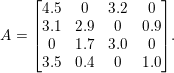 $$\begin{eqnarray}A=\left[\begin{array}{@{}cccc@{}}4.5 & 0 & 3.2 & 0\\ 3.1 & 2.9 & 0 & 0.9\\ 0 & 1.7 & 3.0 & 0\\ 3.5 & 0.4 & 0 & 1.0\\ \end{array}\right]\!.\end{eqnarray}$$

Exact numerical cancellation is rare, and most algorithms ignore it. An entry in the data structure that is computed but found to be numerically zero is still called a ‘non-zero’, by convention. Leaving these entries in the matrix leads to much simpler algorithms and more elegant graph-theoretical statements about the algorithms.
Accessing a column of this data structure is very fast, but extracting a given row is very costly. Algorithms that operate on such a data structure must be designed accordingly. Likewise, modifying the non-zero pattern of a compressed-column matrix is not trivial. Deleting or adding single entry takes  $O(|A|)$ time, if gaps are not tolerated between columns. MATLAB uses the compressed-column data structure for its sparse matrices, with the extra constraint that no numerically zero entries are stored Gilbert, Moler and Schreiber (Reference Gilbert, Moler and Schreiber1992). McNamee (Reference Mcnamee1971, Reference Mcnamee1983a, Reference Mcnamee1983b) provided the first published software for basic sparse matrix data structures and operations (multiply, add, and transpose). Gustavson (Reference Gustavson, Rose and Willoughby1972) summarizes a range of methods and data structures, including how this data structure can be modified dynamically to handle fill-in during factorization.
Finite element methods generate a matrix as a collection of elements, or dense submatrices. A solver dedicated to solving finite element problems will often accept its input in this form. Each element requires a non-zero pattern of the rows and columns it affects. The complete matrix is a summation of the elements, and two or more elements may contribute to the same matrix entry. Thus, it is a common practice for any data structure that any duplicate entries be summed, which can be done in linear time.
2.2 Matrix–vector multiplication
One of the simplest sparse matrix algorithms is matrix–vector multiplication,  $z=Ax+y$, where
 $y$ and
 $x$ are dense vectors and
 $A$ is sparse. If
 $A$ is split into
 $n$ column vectors, the result
 $z=Ax+y$ is
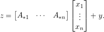 $$\begin{eqnarray}z=\left[\begin{array}{@{}ccc@{}}A_{\ast 1} & \cdots \, & A_{\ast n}\end{array}\right]\left[\begin{array}{@{}c@{}}x_{1}\\ \vdots \\ x_{n}\end{array}\right]+y.\end{eqnarray}$$
Allowing the result to overwrite the input vector  $y$, the
 $j$th iteration computes
 $y=y+A_{\ast j}x_{j}$. The 1-based pseudocode for computing
 $y=Ax+y$ is given below.
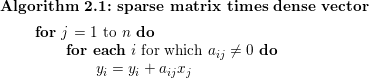
Algorithm 2.1 illustrates the use of gather/scatter operations, which are very common in sparse direct methods. The innermost loop has the form y[i[k]] = y[i[k]] + a[k]*x[j], which requires both a gather and a scatter. A gather operation is a subscripted subscript appearing on the right-hand side of an assignment statement, of the form s = y[i[k]], where y is a dense vector and s is a scalar. A scatter operation occurs when an expression y[i[k]] appears as the target of an assignment. Gather/scatter operations result in a very irregular access to memory, and are thus very costly. Memory transfers are fastest when access has spatial or temporal locality, although the computations themselves can be pipelined on modern architectures (Lewis and Simon Reference Lewis and Simon1988). One of the goals of supernodal, frontal, and multifrontal methods (Sections 9–11) is to replace most of the irregular gather/scatter operations with regular operations on dense submatrices.
Sparse matrix–vector multiplication is a common kernel in iterative methods, although they typically use a compressed-row format (or one of many other specialized data structures), since it results in a faster method because of memory traffic. It requires only a gather operation, not the gather/scatter of Algorithm 2.1.
2.3 Transpose
The algorithm for transposing a sparse matrix ( $C=A^{T}$) is very similar to the method for converting a triplet form to a compressed-column form. The algorithm computes the row counts of A and the cumulative sum to obtain the row pointers. It then iterates over each non-zero entry in A, placing the entry in its appropriate row vector. Transposing a matrix twice results in sorted row indices. Gustavson (Reference Gustavson1978) describes algorithms for matrix multiply (
 $C=AB$) and permuted transpose (
 $C=(PAQ)^{T}$ where
 $P$ and
 $Q$ are permutation matrices). The latter takes linear time (
 $O(n+|A|)$ where
 $n$ is the matrix dimension and
 $|A|$ is the number of non-zeros).
2.4 Matrix multiplication and addition
Algorithms are tuned to their data structures. For example, if two sparse matrices  $A$ and
 $B$ are stored in compressed-column form, then a matrix multiplication
 $C=AB$ where
 $C$ is
 $m\times n$,
 $A$ is
 $m\times k$, and
 $B$ is
 $k\times n$, should access
 $A$ and
 $B$ by column, and create
 $C$ one column at a time. If
 $C_{\ast j}$ and
 $B_{\ast j}$ denote column
 $j$ of
 $C$ and
 $B$, then
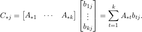
 $C_{\ast j}=AB_{\ast j}$. Splitting
 $A$ into its
 $k$ columns and
 $B_{\ast j}$ into its
 $k$ individual entries results in
 $$\begin{eqnarray}C_{\ast j}=\left[\begin{array}{@{}ccc@{}}A_{\ast 1} & \cdots \, & A_{\ast k}\end{array}\right]\left[\begin{array}{@{}c@{}}b_{1j}\\ \vdots \\ b_{kj}\end{array}\right]=\mathop{\sum }_{t=1}^{k}A_{\ast t}b_{tj}.\end{eqnarray}$$
The non-zero pattern of  $C$ is given by the following theorem.
Theorem 2.1 (Gilbert Reference Gilbert1994).
The non-zero pattern of  $C_{\ast j}$ is the set union of the non-zero pattern of
 $A_{\ast t}$ for all
 $t$ for which
 $b_{tj}$ is non-zero. If
 ${\mathcal{C}}_{j}$,
 ${\mathcal{A}}_{i}$, and
 ${\mathcal{B}}_{j}$ denote the set of row indices of non-zero entries in
 $C_{\ast j}$,
 $A_{\ast t}$, and
 $B_{\ast j}$, then (ignoring numerical cancellation)
 $$\begin{eqnarray}{\mathcal{C}}_{j}=\mathop{\bigcup }_{t\in {\mathcal{B}}_{j}}{\mathcal{A}}_{t}.\end{eqnarray}$$
A matrix multiplication algorithm must compute both the numerical values  $C_{\ast j}$ and the pattern
 ${\mathcal{C}}_{j}$, for each column
 $j$. A variant of Gustavson’s algorithm below uses a temporary dense vector
 $x$ to construct each column, and a flag vector
 $w$, both of size
 $n$ and both initially zero (Gustavson Reference Gustavson1978). The matrix
 $C$ grows one entry at a time, column by column. The three ‘for each …’ loops access a single column of a sparse matrix in a compressed-column data structure.
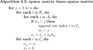
As stated, this algorithm requires a dynamic allocation of  $C$ since it starts out as empty and grows one entry at a time to a size that is not known a priori. Computing the pattern
 ${\mathcal{C}}$ or even just its size is actually much harder than computing the pattern or size of a sparse factorization. The latter is discussed in Section 4. Another approach computes the size of the pattern
 ${\mathcal{C}}$ in an initial symbolic pass, followed by the second numeric pass above, which allows for
 $C$ to be statically allocated. The first pass and second passes take the same time, in a big-
 ${\mathcal{O}}$ sense. For sparse factorization, by contrast, the symbolic analysis is asymptotically faster than the numeric factorization. The time taken by Algorithm 2.2 is
 $O(n+f+|B|)$, where
 $f$ is the number of floating-point operations performed, which is typically dominated by
 $f$.
Matrix addition  $C=A+B$ is very similar to matrix multiplication. The only difference is that two nested ‘for each’ loops above are replaced by two non-nested loops, one that accesses the
 $j$th column of
 $B$ and the other the
 $j$th column of
 $A$.
2.5 Permutations
A sparse matrix must typically be permuted either before or during its numeric factorization, either for reducing fill-in or for numerical stability, or often for both. Fill-in is the introduction of new non-zeros in the factors that do not appear in the corresponding positions in the matrix being factorized. Finding a suitable fill-reducing permutation is discussed in Section 8.
Permutations are typically represented as integer vectors. If  $C=PA$ is to be computed, then the row permutation
 $P$ can be represented as a permutation vector p of size n. If row
 $i$ of
 $A$ becomes the
 $k$th row of
 $C$, then i=p[k]. The inverse permutation is k=invp[i]. Permuting
 $A$ to obtain
 $C$ requires the latter, since a traversal of
 $A$ gives a set of row indices
 $i$ of
 $A$ that must be translated to rows
 $k$ of
 $C$, via the computation k=invp[i]. Column permutations
 $C=AQ$ are most simply done with a permutation vector q where j=q[k] if column
 $j$ of
 $A$ corresponds to column
 $k$ of
 $C$. This allows
 $C$ to be constructed one column at a time, from left to right.
3 Solving triangular systems
Solving a triangular system,  $Lx=b$, where
 $L$ is sparse, square, and lower triangular, is a key mathematical kernel for sparse direct methods. It will be used in Section 5 as part of a sparse Cholesky factorization algorithm, and in Section 6 as part of a sparse LU factorization algorithm. Solving
 $Lx=b$ is also essential for solving
 $Ax=b$ after factorizing
 $A$.
3.1 A dense right-hand side
There are many ways of solving  $Lx=b$ but if
 $L$ is stored as a compressed-column sparse matrix, accessing
 $L$ by columns is the most natural. Assuming
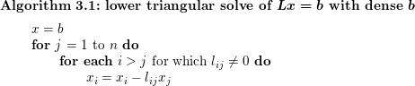
 $L$ has unit diagonal, we obtain a simple Algorithm 3.1, below, that is very similar to matrix–vector multiplication. The vector
 $x$ is accessed via gather/scatter. Solving related systems, such as
 $L^{T}x=b$,
 $Ux=b$, and
 $U^{T}x=b$ (where
 $U$ is upper triangular) is similar, except that the transposed solves are best done by accessing the transpose of the matrix row-by-row, if the matrix is stored in column form.
3.2 A sparse right-hand side
When the right-hand side is sparse, the solution  $x$ is also sparse, and not all columns of
 $L$ take part in the computation since the
 $j$th loop of Algorithm 3.1 can be skipped if
 $x_{j}=0$. Scanning all of
 $x$ for this condition adds
 $O(n)$ to the time complexity, which is not optimal. However, if the set of indices
 $j$ for which
 $x_{j}$ will be non-zero is known, denoted
 ${\mathcal{X}}=\{j\,|\,x_{j}\neq 0\}$, the algorithm is as follows.
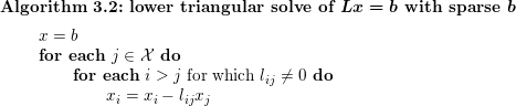
Sparse triangular solve (Davis Reference Davis2006).
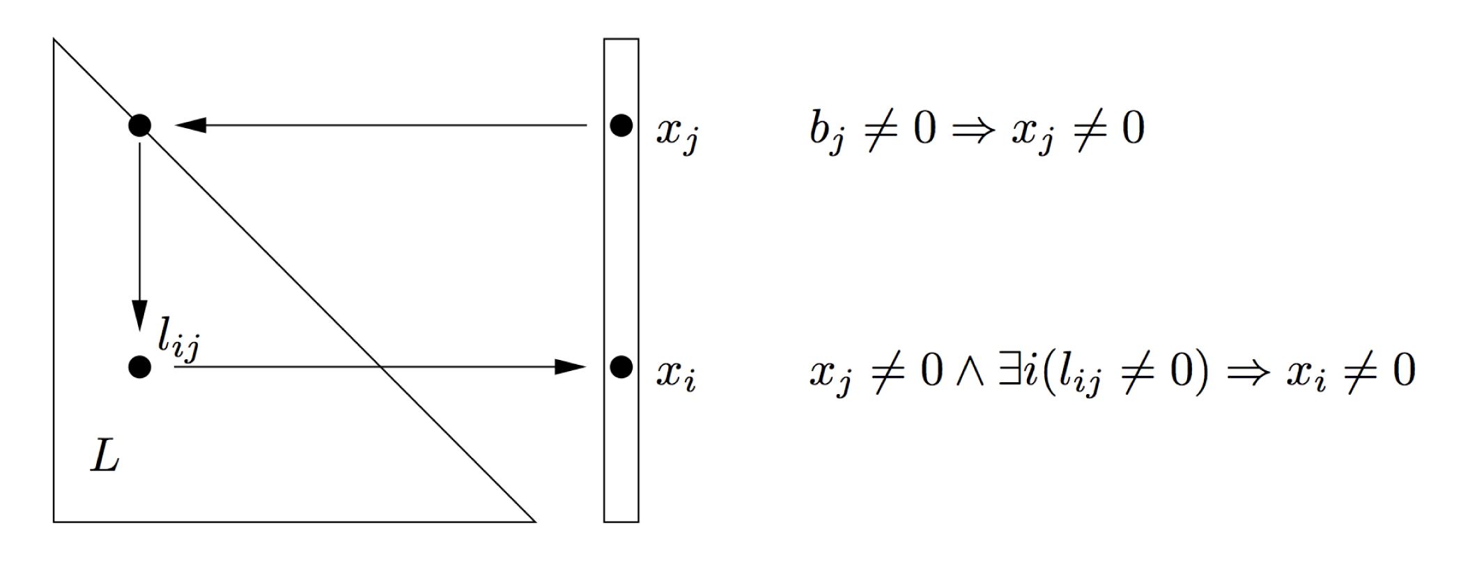
The runtime is now optimal, but  ${\mathcal{X}}$ must be determined first, as Gilbert and Peierls (Reference Gilbert and Peierls1988) describe. Finding
 ${\mathcal{X}}$ requires that we follow a set of implications. Entries in
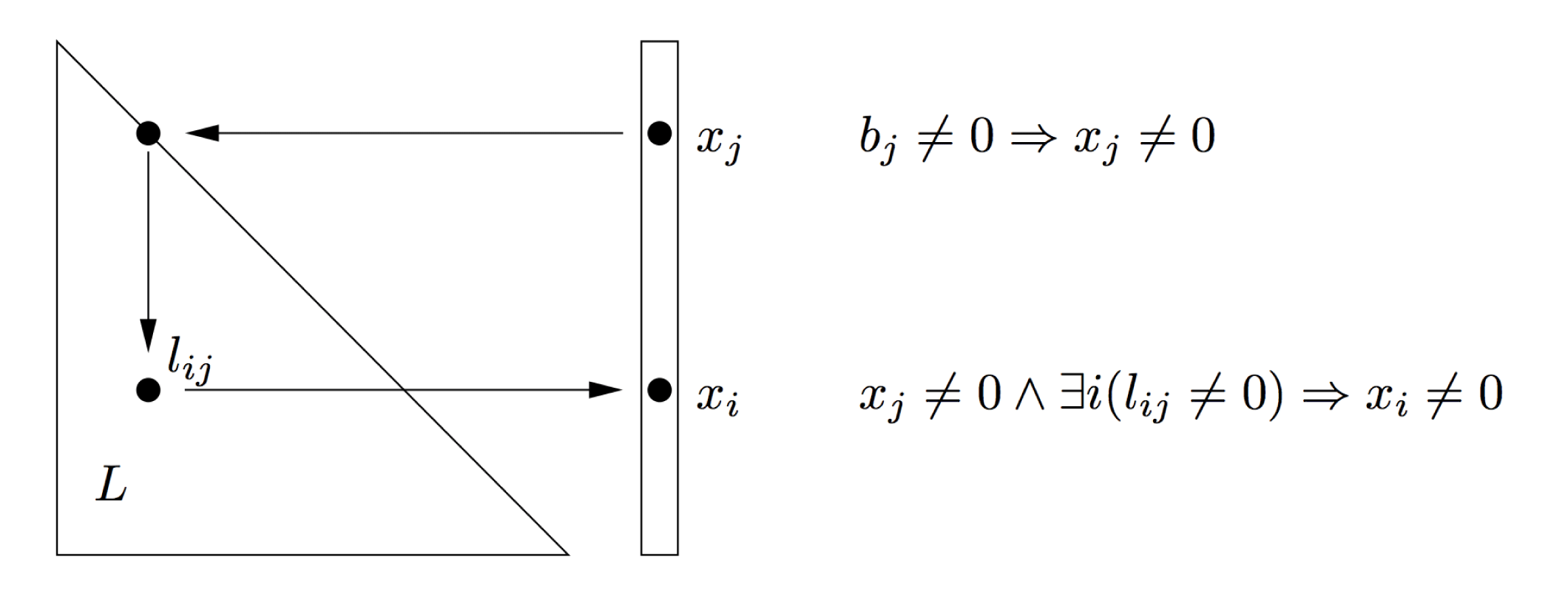
 $x$ become non-zero in two places, the first and last lines of Algorithm 3.2. Neglecting numerical cancellation, rule one states that
 $b_{i}\neq 0\Rightarrow x_{i}\neq 0$, and rule two is
 $x_{j}\neq 0\wedge \exists i(l_{ij}\neq 0)\Rightarrow x_{i}\neq 0$. These two rules lead to a graph traversal problem. Consider a directed acyclic graph
 $G_{L}=(V,E)$ where
 $V=\{1\ldots n\}$ and
 $E=\{(j,i)\,|\,l_{ij}\neq 0\}$. Rule one marks all nodes in
 ${\mathcal{B}}$, the non-zero pattern of
 $b$. Rule two states that if a node is marked, all its neighbours become marked. These rules are illustrated in Figure 3.1. In graph terminology,
 $$\begin{eqnarray}{\mathcal{X}}=\text{Reach}_{L}({\mathcal{B}}).\end{eqnarray}$$
Computing  ${\mathcal{X}}$ requires a depth-first search of the directed graph
 $G_{L}$, starting at nodes in
 ${\mathcal{B}}$. The time taken is proportional to the number of edges traversed, which is exactly equal to the floating-point operation count. A depth-first search computes
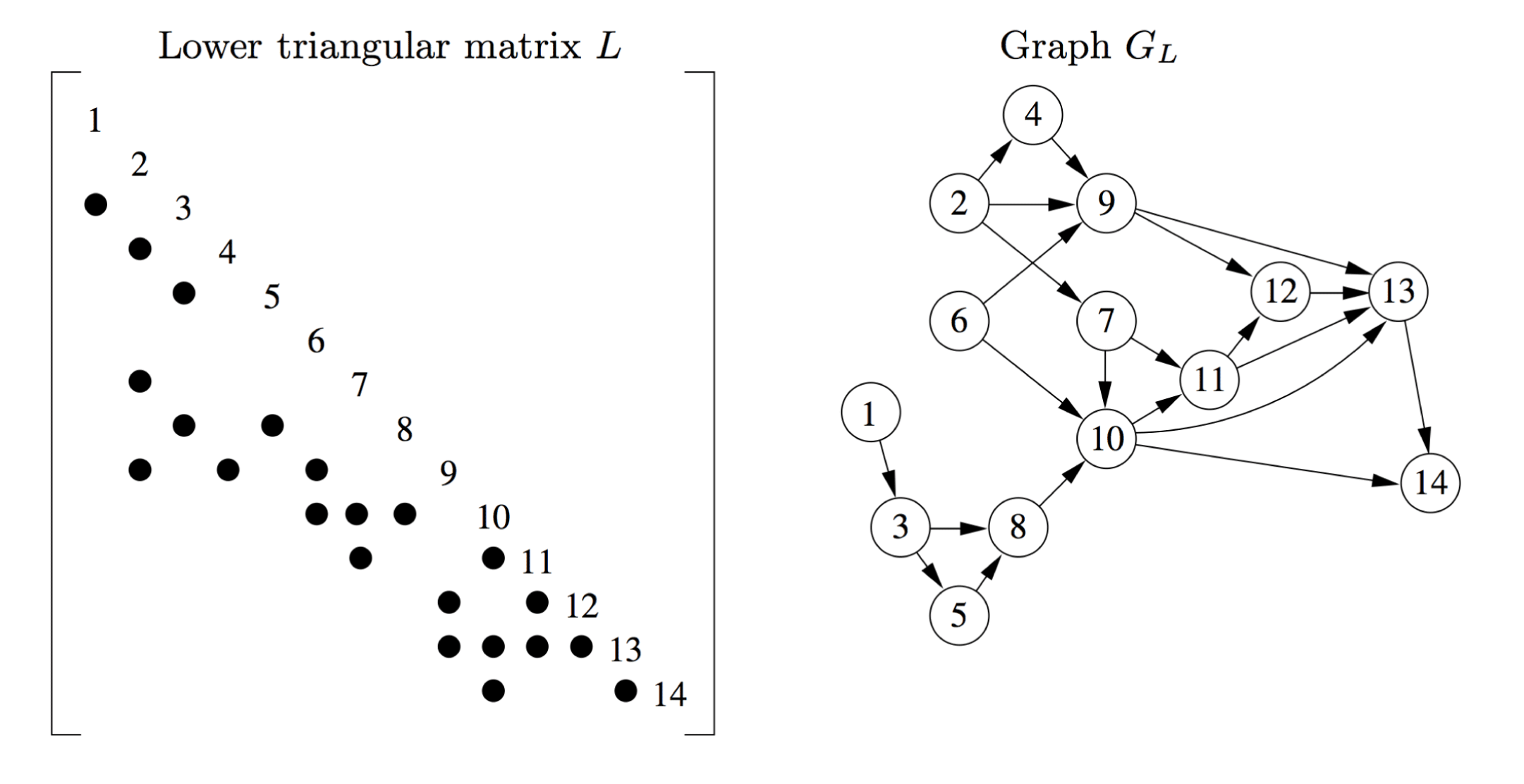
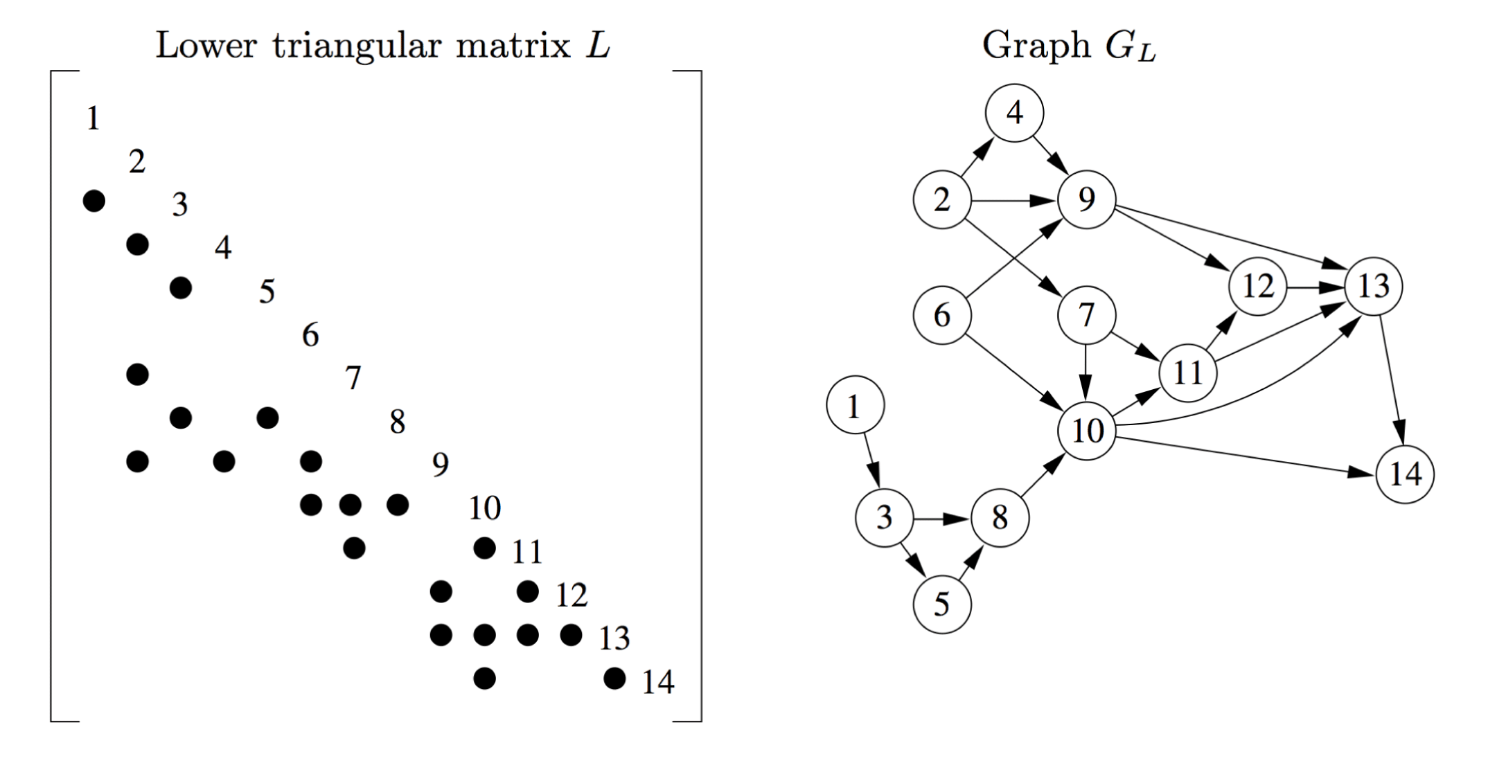
 ${\mathcal{X}}$ in topological order, and performing the numerical solve in that order preserves the numerical dependencies. An example of a triangular solve is shown in Figure 3.2. If
 ${\mathcal{B}}=\{4,6\}$, then in this example
 ${\mathcal{X}}=\{6,10,11,4,9,12,13,14\}$, listed in topological order as produced by the depth-first search. The sparse triangular solve forms the basis of the left-looking sparse LU method presented in Section 6.2. For the parallel triangular solve, see Section 12.2.
Solving  $Lx=b$, where
 $L$,
 $x$, and
 $b$ are sparse (Davis Reference Davis2006).
4 Symbolic analysis
Solving a sparse system of equations,  $Ax=b$, using a direct method starts with a factorization of
 $A$, followed by a solve phase that uses the factorization to solve the system. In all but a few methods, the factorization splits into two phases: a symbolic phase that typically depends only on the non-zero pattern of
 $A$, and a numerical phase that produces the factorization itself. The solve phase uses the triangular solvers as discussed in Section 3.
The symbolic phase is asymptotically faster than the numeric factorization phase, and it allows the numerical phase to be more efficient in terms of time and memory. It also allows the numeric factorization to be repeated for a sequence of matrices with identical non-zero pattern, a situation that often arises when solving non-linear and/or differential equations.
The first step in the symbolic analysis is to find a good fill-reducing permutation. Sparse direct methods for solving  $Ax=b$ do not need to factorize
 $A$, but can instead factorize a permuted matrix:
 $PAQ$ if
 $A$ is unsymmetric, or
 $PAP^{T}$ if it is symmetric. Finding the optimal
 $P$ and
 $Q$ that minimizes memory usage or flop count to compute the factorization is an NP-hard problem (Yannakakis Reference Yannakakis1981), and thus heuristics are used. Fill-reducing orderings are a substantial topic in their own right. Understanding how they work and what they are trying to optimize requires an understanding of the symbolic and numeric factorizations. Thus, a discussion of the ordering topic is postponed until Section 8.
Once the ordering is found, the symbolic analysis finds the elimination tree, and the non-zero pattern of the factorization or its key properties such as the number of non-zeros in each row and column of the factors.
Although the symbolic phase is a precursor for all kinds of factorizations, it is the Cholesky factorization of a sparse symmetric positive definite matrix  $A=LL^{T}$ that is considered first. Much of this analysis applies to the other factorizations as well (QR can be understood via the Cholesky factorization of
 $A^{T}A$, for example). Connections to the other factorization methods are discussed in Sections 6 and 7.
The non-zero pattern of the Cholesky factor  $L$ is represented by an undirected graph
 $G_{L+L^{T}}$, with an edge
 $(i,j)$ if
 $l_{ij}\neq 0$. There are many ways to compute the Cholesky factorization
 $A=LL^{T}$ and the graph
 $G_{L+L^{T}}$, and the algorithms and software discussed in Section 13 reflect these variants. One of the simplest Cholesky factorization algorithms is the up-looking variant, which relies on the sparse sparse triangular solve,
 $Lx=b$. This form of the Cholesky factorization will be used here to derive the elimination tree and the method for finding the row/column counts. Consider a 2
 $\times$ 2 block decomposition
 $LL^{T}=A$,
 $$\begin{eqnarray}\left[\begin{array}{@{}cc@{}}L_{11} & \\ l_{12}^{T} & l_{22}\end{array}\right]\left[\begin{array}{@{}cc@{}}L_{11}^{T} & l_{12}\\ & l_{22}\end{array}\right]=\left[\begin{array}{@{}cc@{}}A_{11} & a_{12}\\ a_{12}^{T} & a_{22}\end{array}\right]\!,\end{eqnarray}$$
where  $L_{11}$ and
 $A_{11}$ are
 $(n-1)\times (n-1)$. These terms can be computed with (1)
 $L_{11}L_{11}^{T}=A_{11}$ (a recursive factorization of the leading submatrix of
 $A$), (2)
 $L_{11}l_{12}=a_{12}$ (a sparse triangular solve for
 $l_{12}$), and (3)
 $l_{12}^{T}l_{12}+l_{22}^{2}=a_{22}$ (a dot product to compute
 $l_{22}$). When the recursion is unrolled, a simple algorithm results that computes each row of
 $L$, one row at a time, starting at row 1 and proceeding to row
 $n$.
Rose (Reference Rose and Read1972) provided the first detailed graph-theoretic analysis of the sparse Cholesky factorization, based on an outer-product formulation. Consider the decomposition
 $$\begin{eqnarray}\left[\begin{array}{@{}cc@{}}l_{11} & \\ l_{21} & L_{22}\end{array}\right]\left[\begin{array}{@{}cc@{}}l_{11} & l_{21}^{T}\\ & L_{22}^{T}\end{array}\right]=\left[\begin{array}{@{}cc@{}}a_{11} & a_{21}^{T}\\ a_{21} & A_{22}\end{array}\right]\!,\end{eqnarray}$$
where the (22)-blocks have dimension  $n-1$. This leads to a factorization computed with (1)
 $l_{11}=\sqrt{a_{11}}$, a scalar square-root, (2)
 $l_{12}=a_{21}/l_{22}$, which divides a sparse column vector by scalar, and (3) the Cholesky factorization
 $L_{22}L_{22}^{T}=A_{22}-l_{21}l_{21}^{T}$. The undirected graph of the Schur complement,
 $A_{22}-l_{21}l_{21}^{T}$, has a special structure. Node 1 is gone, and removing it causes extra edges to appear (fill-in), resulting in a clique of its neighbours. That is, the graph of
 $l_{21}l_{21}^{T}$ is a clique of the neighbours of node 1. As a result, the graph of
 $L+L^{T}$ is chordal, in which every cycle of length greater than 3 contains a chord. George and Liu (Reference George and Liu1975) consider the special case when all the entries in the envelope of the factorization become all non-zero (defined in Section 8.2). If a matrix can be permuted so that no fill-in occurs in its factorization, it is said to have a perfect elimination ordering; the graph of
 $L+L^{T}$ is one such matrix (Rose Reference Rose and Read1972, Bunch Reference Bunch and Traub1973, Duff and Reid Reference Duff and Reid1983b). Tarjan (Reference Tarjan, Bunch and Rose1976) surveys the use of graph theory in symbolic factorization and fill-reducing ordering methods, including the unsymmetric case.
Fill-in can be catastrophic, causing the sparse factorization to require  $O(n^{2})$ memory and
 $O(n^{3})$ time. This occurs for nearly all random matrices (Duff Reference Duff1974a) but almost never for matrices arising from real applications. The moral of this observation is that performance results of sparse direct methods with random sparse matrices should always be suspect. Trustworthy results require matrices arising from real applications, or from matrix generators such as two- or three-dimensional meshes that mimic real applications. As a result, collecting matrices that arise in real applications is crucial for the development of all sparse direct methods (Duff and Reid Reference Duff, Reid and Fosdick1979a, Duff et al. Reference Duff, Grimes and Lewis1989a, Davis and Hu Reference Davis and Hu2011). Inverting an entire sparse matrix does result in catastrophic fill-in, which is why it is never computed to solve
 $Ax=b$ (Duff, Erisman, Gear and Reid Reference Duff, Erisman, Gear and Reid1988).
4.1 Elimination tree
The elimination tree (or etree) appears in many sparse factorization algorithms and in many related theorems. It guides the symbolic analysis and provides a framework for numeric factorization, both parallel and sequential.
Consider equation (4.1), applied to the leading  $k\times k$ submatrix of
 $A$. The vector
 $l_{12}$ is computed with a sparse triangular solve,
 $L_{11}l_{12}=a_{12}$, and its transpose becomes the
 $k$th row of
 $L$. Its non-zero pattern is thus
 ${\mathcal{L}}_{k}=\text{Reach}_{G_{k-1}}({\mathcal{A}}_{k})$, where
 $G_{k-1}$ is the directed graph of
 $L_{11}$,
 ${\mathcal{L}}_{k}$ is the non-zero pattern of the
 $k$th row of
 $L$, and
 ${\mathcal{A}}_{k}$ is the non-zero pattern of the upper triangular part of the
 $k$th column of
 $A$.
The depth-first search of  $G_{k-1}$ is sufficient for computing
 ${\mathcal{L}}_{k}$, but a simpler method exists, taking only
 $O(|{\mathcal{L}}_{k}|)$ time. It is based on a pruning of the graph
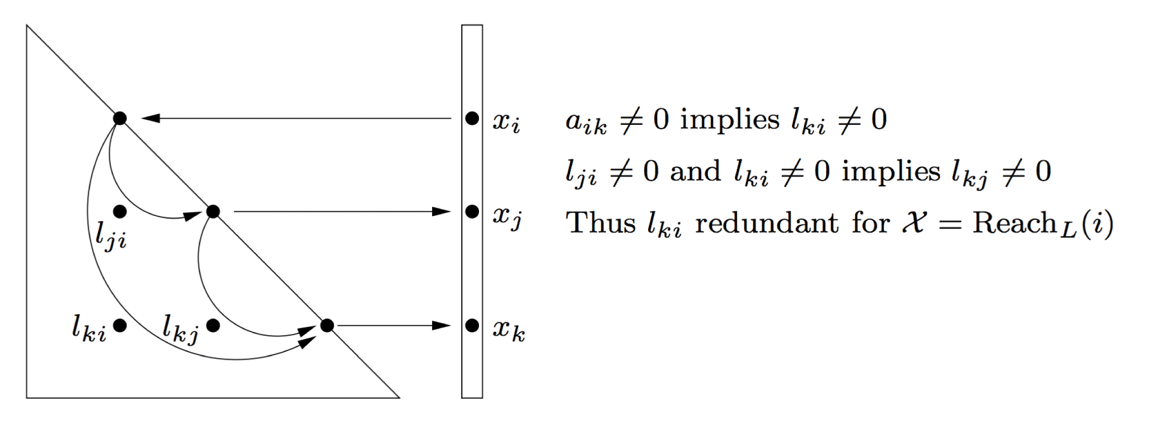
 $G_{k-1}$ (Figure 4.1). Computing the
 $k$th row of
 $L$ requires a triangular solve of
 $L_{1:k-1,1:1-k}x=b$, where the right-hand
 $b$ is the
 $k$ row of
 $A$. Thus, if
 $a_{ik}$ is non-zero, so is
 $b_{i}$ and
 $x_{i}$. This entry
 $x_{i}$ becomes
 $l_{ki}$ and thus
 $a_{ik}\neq 0$ implies
 $x_{i}=l_{ki}\neq 0$.
Pruning the directed graph  $G_{L}$ yields the elimination tree.
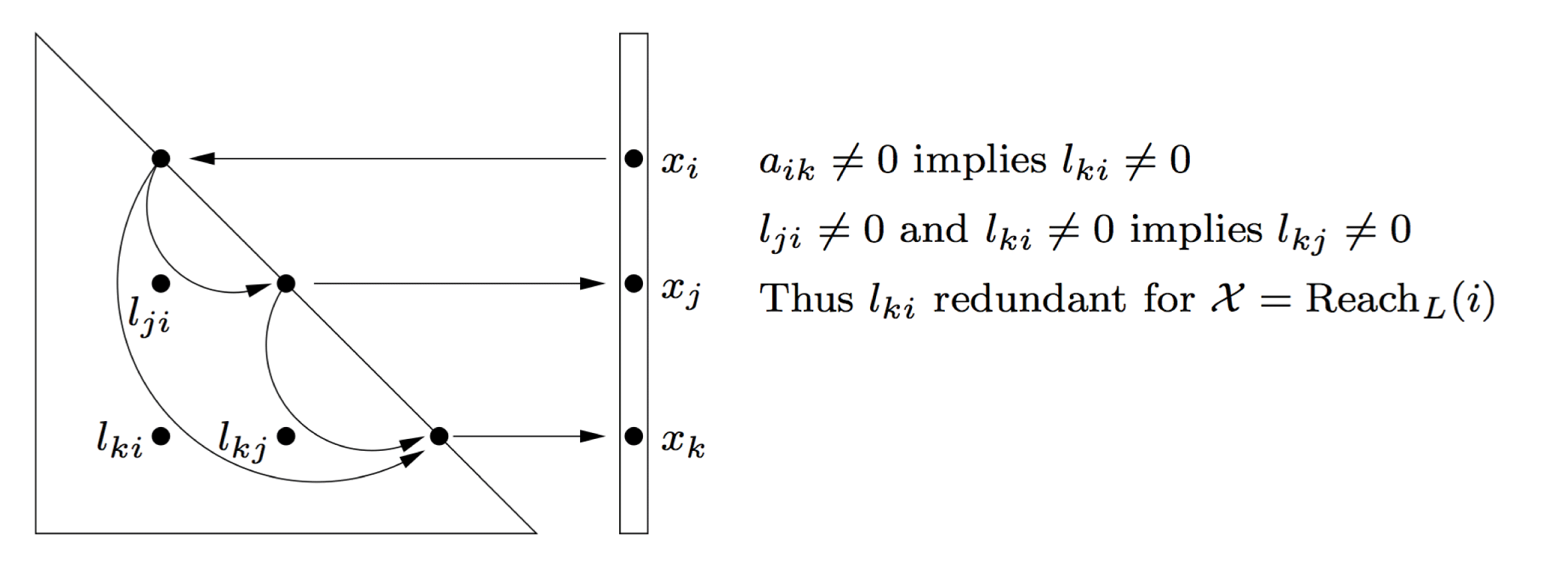
If there is another non-zero  $l_{ji}$ with
 $j<k$, then there is an edge from
 $i$ to
 $j$ in the graph, and so when doing the graph traversal from node
 $i$, node
 $j$ will be reached. As a result,
 $x_{j}\neq 0$. This becomes the entry
 $l_{kj}$, and thus the existence of a pair of non-zeros
 $l_{ji}$ and
 $l_{ki}$ implies that
 $l_{kj}$ is non-zero (Parter Reference Parter1961). Outer-product Gaussian elimination is another way to look at this (
 $A=LU$): for a symmetric matrix
 $A$, two non-zero entries
 $u_{ij}$ and
 $l_{ki}$ cause
 $l_{kj}$ to become non-zero when the
 $i$th pivot entry is eliminated.
For the sparse triangular solve, if the graph traversal starts at node  $i$, it will see both nodes
 $j$ and
 $k$. The reach of node
 $i$ is not changed if the edge
 $(i,k)$ is ignored; it can still reach
 $k$ from a path of length two:
 $i$ to
 $j$ to
 $k$. As a result, any edge
 $(i,k)$ corresponding to the non-zero
 $l_{ki}$ can be ignored in the graph search, just so long as there is another non-zero
 $l_{ji}$ above it in the same column. Only the first off-diagonal entry is needed, that is, the smallest
 $j>i$ for which
 $l_{ji}$ is non-zero. Pruning all but this edge results in the same reach (3.1) for the triangular solve,
 $L_{11}l_{12}=a_{12}$, but the resulting structure is faster to traverse. A directed acyclic graph with at most one outgoing edge per node is a tree (or forest). This is the elimination tree. It may actually be a forest, but by convention is still called the elimination tree.
In terms of the graph of  $A$, if there is a path of length two between the two nodes
 $k$ and
 $j$, where the intermediate node is
 $i<\min (k,j)$, then this causes the edge
 $(k,j)$ to appear in the filled graph. Rose, Tarjan and Lueker (Reference Rose, Tarjan and Lueker1976) generalized Parter’s result in their path lemma:
 $l_{ij}$ is non-zero if and only if there is a path path
 $i{\rightsquigarrow}j$ in
 $A$ where all intermediate nodes are numbered less than
 $\min (i,j)$.
The elimination tree is based on the pattern of  $L$, but it can be computed much more efficiently without finding the pattern of
 $L$, in time essentially linear in
 $|A|$ (Liu Reference Liu1986a, Schreiber Reference Schreiber1982). The algorithm relies on the quick traversal of paths in the tree as it is being constructed. A key theorem by Liu states that if
 $a_{ki}\neq 0$ (where
 $k>i$), then
 $i$ is a descendant of
 $k$ in the elimination tree (Liu Reference Liu1990). The tree is constructed by ensuring this property holds for each entry in
 $A$.
Let  ${\mathcal{T}}$ denote the elimination tree of
 $L$, and let
 ${\mathcal{T}}_{k}$ denote the elimination tree of submatrix
 $L_{1\ldots k,1\ldots k}$, the first
 $k$ rows and columns of
 $L$.
The tree is constructed incrementally, for each leading submatrix of  $A$. That is, the tree
 ${\mathcal{T}}_{k}$ for the matrix
 $A_{1..k,1..k}$ is constructed from
 ${\mathcal{T}}_{k-1}$. For each entry
 $a_{ki}\neq 0$, it suffices to ensure that
 $i$ is a descendant of
 $k$ in the next tree
 ${\mathcal{T}}_{k}$. Walking the path from
 $i$ to a root
 $t$ in
 ${\mathcal{T}}_{k-1}$ means that
 $t$ must be a child of
 $k$ in
 ${\mathcal{T}}_{k}$. This path could be traversed one node at a time, but it is much more efficient to compress the paths as they are found, to speed up subsequent traversals. Future traversals from
 $i$ must arrive at
 $k$, so as the path is traversed, each node along the path is given a shortcut to its ancestor
 $k$. This method is an application of the disjoint-set-union-find algorithm of Tarjan (Reference Tarjan1975) (see also Cormen et al. Reference Cormen, Leiserson and Rivest1990). Thus, its runtime is essentially linear in the number of entries in
 $A$ (this is called nearly
 $O(|A|)$). This is much faster than
 $O(|L|)$, and it means that the tree can be computed prior to computing the non-zero pattern of
 $L$, and then used to construct the pattern of
 $L$ or to explore its properties.
The column elimination tree is the elimination tree of  $A^{T}A$, and is used in the QR and LU factorization algorithms. It can be computed without forming
 $A^{T}A$, also in nearly
 $O(|A|)$ time. Row
 $i$ of
 $A$ creates a dense submatrix, or clique, in the graph of
 $A^{T}A$. To speed up the construction of the tree without forming the graph of
 $A^{T}A$ explicitly, a sparser graph is used, in which each clique is replaced with a path amongst the nodes in the clique. The resulting graph/matrix has the same Cholesky factor and the same elimination tree as
 $A^{T}A$.
Once the tree is found, some algorithms and many theorems require it to be postordered. In a postordered tree, the  $d$ proper descendants of any node
 $k$ are numbered
 $k-d$ to
 $k-1$. If the resulting node renumbering is written as a permutation matrix
 $P$, then the filled graph of
 $A$ and
 $PAP^{T}$ are isomorphic (Liu Reference Liu1990). In other words, the two Cholesky factorizations have the same number of non-zeros and require the same amount of work. Their elimination trees are also isomorphic. Even if the symbolic or numeric factorization does not require a postordering of the etree, doing so makes the computations more regular by placing similar submatrices close to each other, thus improving memory traffic and speeding up the work (Liu Reference Liu1987c).
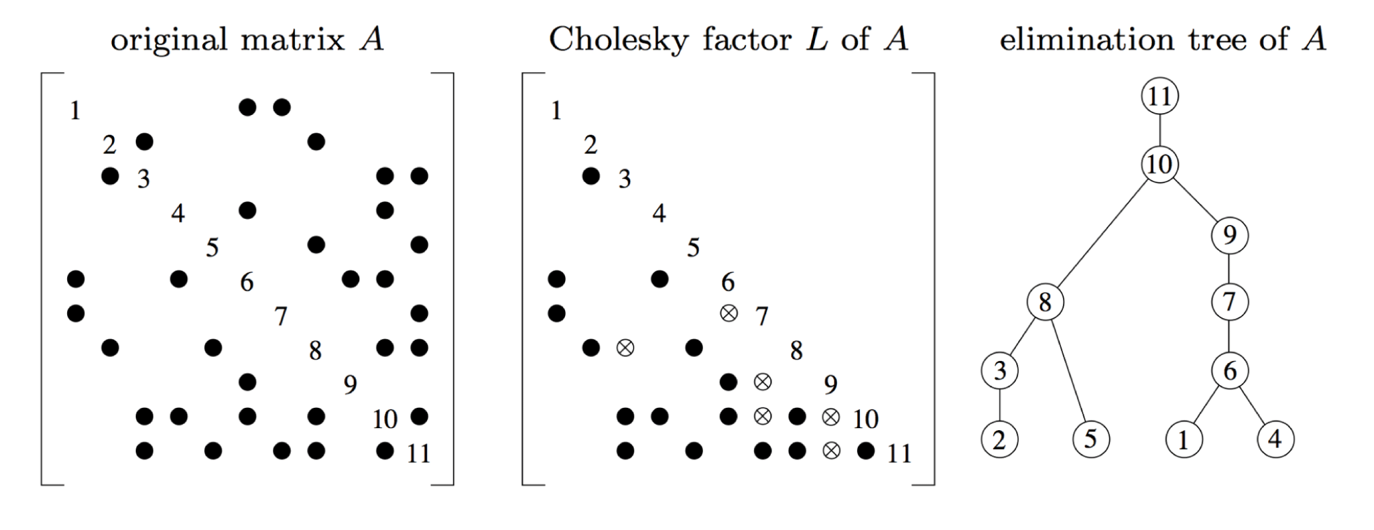
Example matrix  $A$, factor
 $L$, and elimination tree. Fill-in entries in
 $L$ are shown as circled x’s (Davis Reference Davis2006).
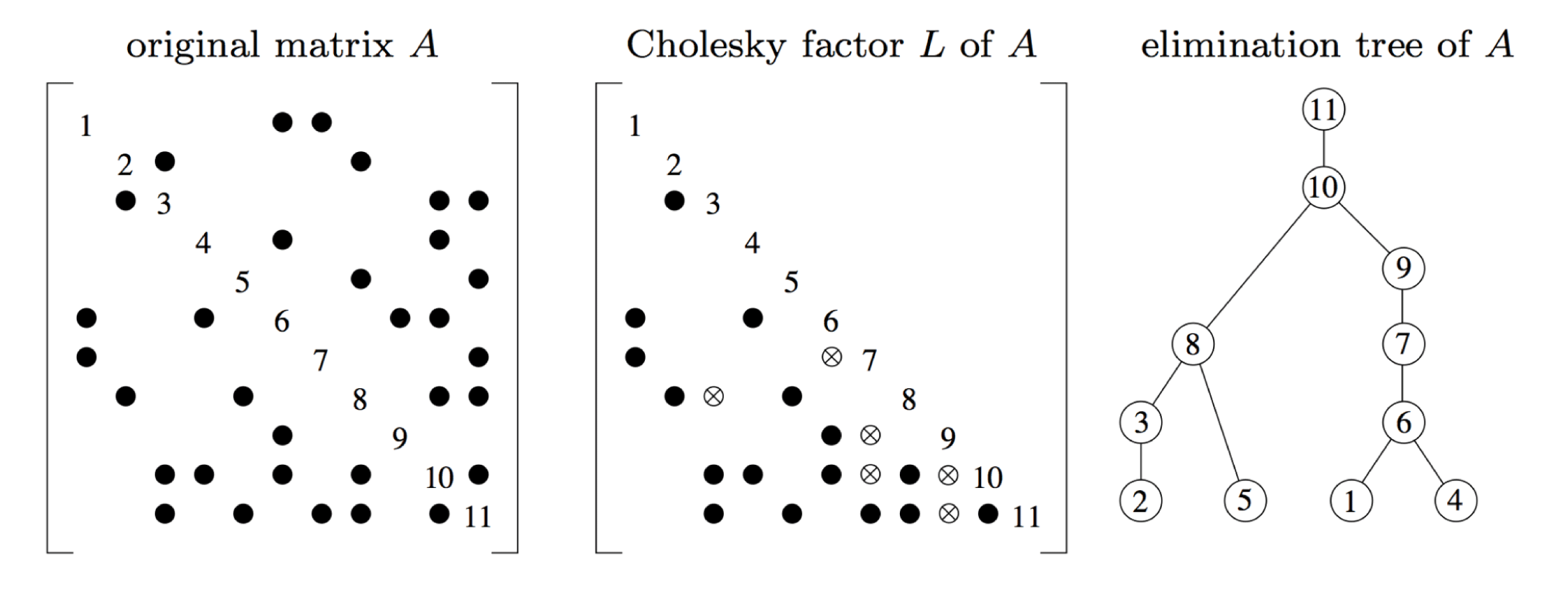
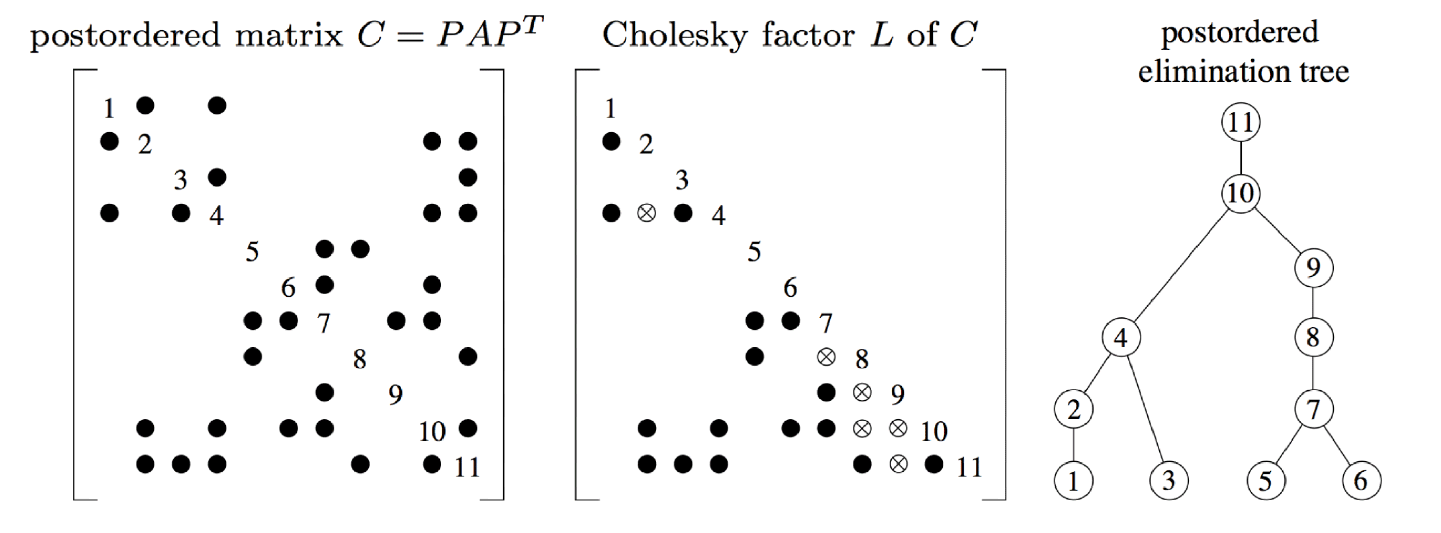
Figure 4.2 shows a matrix  $A$, its Cholesky factor
 $L$, and its elimination tree
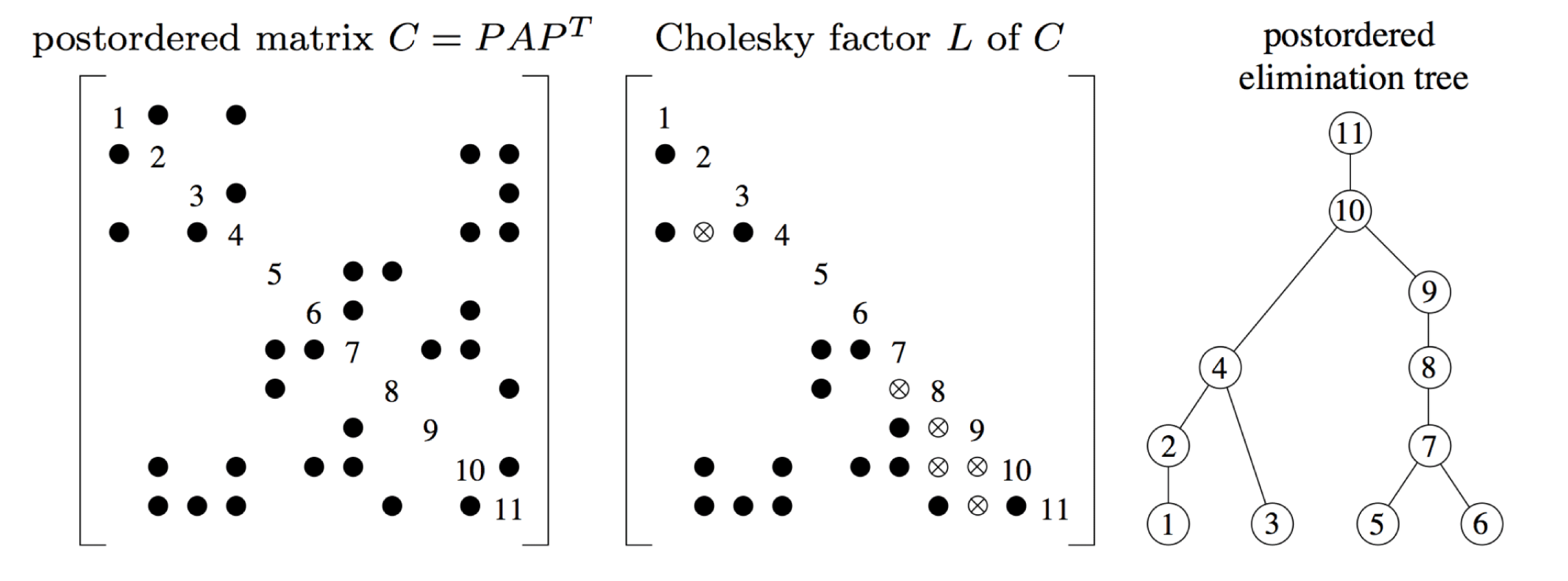
 ${\mathcal{T}}$. Figure 4.3 illustrates the matrix
 $PAP^{T}$, its Cholesky factor, and its elimination tree, where
 $P$ is the postordering of the elimination tree in Figure 4.2.
After elimination tree postordering (Davis Reference Davis2006).
The elimination tree is fundamental to sparse matrix computations; Liu (Reference Liu1990) describes its many uses. Jess and Kees (Reference Jess and Kees1982) applied a restricted definition of the tree for matrices  $A$ that had perfect elimination orderings, and Duff and Reid (Reference Duff and Reid1982) defined a related tree for the multifrontal method (Section 11). The elimination tree was first formally defined by Schreiber (Reference Schreiber1982). Kumar, Kumar and Basu (Reference Kumar, Kumar and Basu1992) present a parallel algorithm for computing the tree, and for symbolic factorization (Section 4.3).
4.2 Row and column counts
The row/column counts for a Cholesky factorization are the number of non-zeros in each row/column of  $L$. These can be found without actually computing the pattern of
 $L$, and in time that is nearly
 $O(|A|)$, by using just the elimination tree and pattern of
 $A$. The column count is useful for laying out a good data structure for
 $L$, and row counts are helpful in determining data dependencies for parallel numeric factorization.
4.2.1 Row counts and row subtrees
The  $k$th row subtree,
 ${\mathcal{T}}^{k}$, consists of a subtree of
 ${\mathcal{T}}$ and defines the non-zero pattern of the
 $k$th row of
 $L$. Each node
 $j$ in
 ${\mathcal{T}}^{k}$ corresponds to a non-zero
 $l_{kj}$. Its leaves are a subset of the
 $k$th row of the lower triangular part of
 $A$. The root of the tree is
 $k$. It is actually a tree, not a forest, and its nodes are the same as those traversed in the sparse lower triangular solve for the
 $k$th step of the up-looking Cholesky factorization. Since the tree can be found without finding the pattern of
 $L$, and since the pattern of
 $A$ is also known, the
 $k$th row subtree precisely defines the non-zero pattern of the
 $k$th row of
 $L$, without the need for storing each entry explicitly.
One simple but non-optimal method for computing the row and column counts is to just traverse each subtree and determine its size using the sparse triangular solve. The size of the tree  ${\mathcal{T}}^{k}$ is number of non-zeros in row
 $k$ of
 $L$ (the row count). Visiting a node
 $j$ in
 ${\mathcal{T}}^{k}$ adds one to the column count of
 $j$. This method is simple to understand, but it takes
 $O(|L|)$ time.
The time can be reduced to nearly linear in  $|A|$ (Gilbert, Li, Ng and Peyton Reference Gilbert, Li, Ng and Peyton2001, Gilbert, Ng and Peyton Reference Gilbert, Ng and Peyton1994). The basic idea is to decompose each row subtree into a set of disjoint paths, each starting with a leaf node and terminating at the least common ancestor of the current leaf and the prior leaf node. The paths are not traversed one node at a time. Instead, the lengths of these paths are found via the difference in the levels of their starting and ending nodes, where the level of a node is its distance from the root. The row count algorithm exploits the fact that all subtrees are related to each other; they are all subtrees of the elimination tree. Summing up the sizes of these disjoint paths gives the row counts.
The row count algorithm postorders the elimination tree, and then finds the level and first descendant of each node, which is the lowest numbered descendant of each node. This phase takes  $O(n)$ time.
The next step traverses all row subtrees, considering column (node)  $j$ in each row subtree in which it appears (that is, all non-zeros
 $a_{ij}$ in column
 $j$, starting at column
 $j=1$ and proceeding to
 $j=n$). If
 $j$ is a leaf in the
 $i$th row subtree, then the least common ancestor
 $c$ of this node and the prior leaf seen in the
 $i$th row subtree define a unique disjoint path, starting at
 $j$ and preceding up to but not including
 $c$. Finding
 $c$ relies on another application of the disjoint-set-union-find algorithm. Once
 $c$ is found, the length of the path from
 $j$ to the child of
 $c$ can be found quickly by taking the difference of the levels
 $j$ and
 $c$.
However, not all entries  $a_{ij}$ are leaves
 $j$ in
 ${\mathcal{T}}^{i}$. The subset of
 $A$ that contains just leaves of row subtrees is called the skeleton matrix. The factorization of skeleton matrix of
 $A$ has the same non-zero pattern as
 $A$ itself. The skeleton is found by looking at the first descendants of the nodes in the tree. When the entry
 $a_{ij}$ is considered, node
 $j$ is a leaf of the
 $i$th row subtree,
 ${\mathcal{T}}^{i}$, if (and only if) the first descendant of
 $j$ is larger than any first descendant yet seen in that subtree.
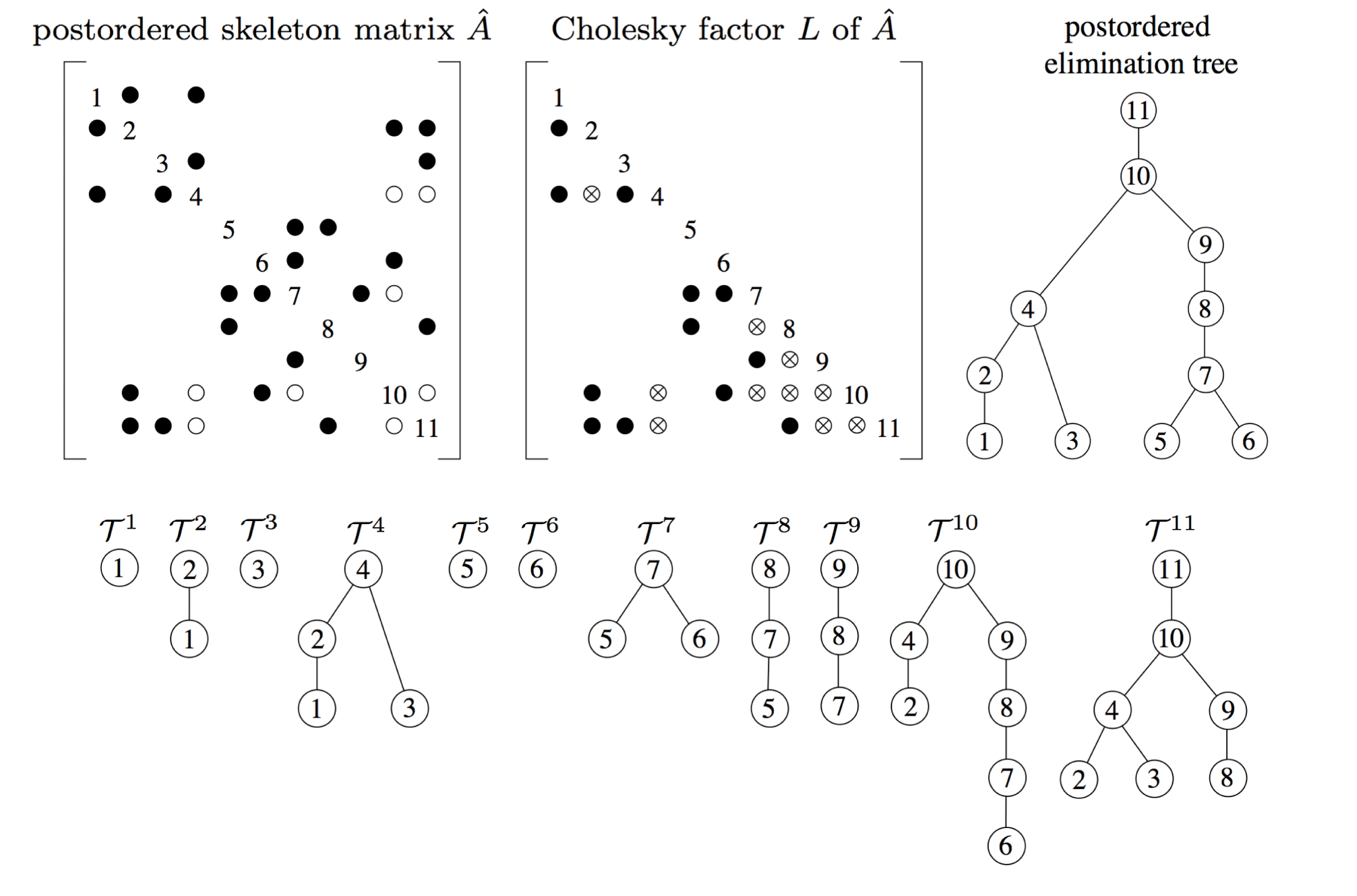
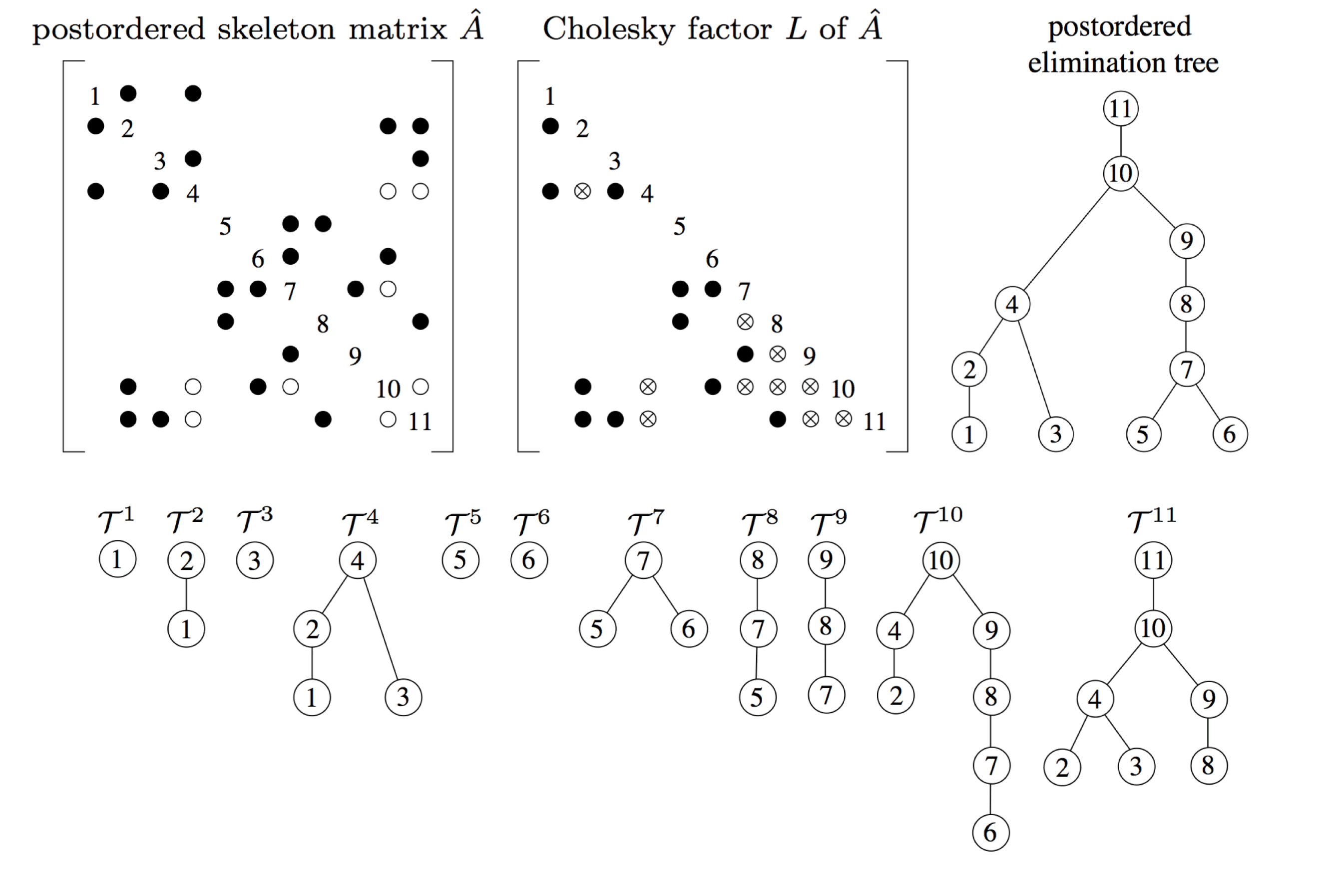
Figure 4.4 shows the postordered skeleton matrix of  $A$, denoted
 $\widehat{A}$, its factor
 $L$, its elimination tree
 ${\mathcal{T}}$, and the row subtrees
 ${\mathcal{T}}^{1}$ to
 ${\mathcal{T}}^{11}$ (compare with Figure 4.3). Entries in the skeleton matrix are shown as dark circles. A white circle denotes an entry in
 $A$ that is not in the skeleton matrix
 $\widehat{A}$.
Skeleton matrix, factor  $L$, elimination tree, and the row subtrees (Davis Reference Davis2006).
The first disjoint path found in the  $i$th row subtree goes from
 $j$ up to
 $i$. Subsequent disjoint paths are defined by the pair of nodes
 $p$ and
 $j$, where
 $p$ is the prior entry
 $a_{ip}$ in the skeleton matrix, and also the prior leaf seen in this subtree. These two nodes define the unique disjoint path from
 $j$ to the common ancestor
 $c$ of
 $p$ and
 $j$. Summing up the lengths of these disjoint paths gives the number of nodes in the
 $i$th row subtree, which is the number of entries in row
 $i$ of
 $L$.
Liu (Reference Liu1986a) defined the row subtree and the skeleton matrix and used these concepts to create a compact data structure that represents the pattern of the Cholesky factor  $L$ row-by-row using only
 $O(A)$ space, holding just the skeleton matrix and the elimination tree. Bank and Smith (Reference Bank and Smith1987) present a symbolic analysis algorithm in which the
 $i$th iteration traverses the
 $i$th row subtree, one disjoint path at a time, in the same manner as the symbolic up-looking Algorithm 4.1, except that it computes the elimination tree on the fly. They do not use the phrase ‘row subtree’ nor do they use the term elimination tree. However, their function
 $m(i)$ is a representation of the elimination tree since
 $m(i)$ is identical to the parent of
 $i$. Their algorithm computes the row counts and the elimination tree in
 $O(|L|)$ time.
4.2.2 Column counts
We now consider how to determine the number of non-zeros in each column of  $L$. Let
 ${\mathcal{L}}_{j}$ denote the non-zero pattern of the
 $j$th column of
 $L$, and let
 ${\mathcal{A}}_{j}$ denote the pattern of the
 $j$th column of the strictly lower triangular part of
 $A$. Let
 $\widehat{{\mathcal{A}}}_{j}$ denote entries in the same part of the skeleton matrix
 $\widehat{A}$. George and Liu (Reference George and Liu1981) show that
 ${\mathcal{L}}_{j}$ is the union of its children in the elimination tree, plus the original entries in
 $A$:
 $$\begin{eqnarray}{\mathcal{L}}_{j}={\mathcal{A}}_{j}\cup \{j\}\cup \biggl(\mathop{\bigcup }_{j=\text{parent}(c)}{\mathcal{L}}_{c}\setminus \{c\}\biggr).\end{eqnarray}$$
A key corollary by Schreiber (Reference Schreiber1982) states that the non-zero pattern of the  $j$th column of
 $L$ is a subset of the path
 $j{\rightsquigarrow}r$ from
 $j$ to the root of the elimination tree
 ${\mathcal{T}}$. The column counts are the sizes of each of these sets,
 $|{\mathcal{L}}_{j}|$. If
 $j$ is a leaf in
 ${\mathcal{T}}$, then the column count is simple:
 $|{\mathcal{L}}_{j}|=|{\mathcal{A}}_{j}|+1=|\widehat{{\mathcal{A}}}_{j}|+1$. Let
 $e_{j}$ denote the number of children of
 $j$ in
 ${\mathcal{T}}$. When
 $j$ is not a leaf, the skeleton entries are leaves of their row subtrees, and do not appear in any child, and thus
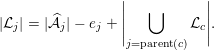 $$\begin{eqnarray}|{\mathcal{L}}_{j}|=|\widehat{{\mathcal{A}}}_{j}|-e_{j}+\left|\mathop{\bigcup }_{j=\text{parent}(c)}{\mathcal{L}}_{c}\right|.\end{eqnarray}$$
Suppose there were an efficient way to find the overlap  $o_{j}$ between the children
 $c$ in (4.4), replacing the set union with a summation:
 $$\begin{eqnarray}|{\mathcal{L}}_{j}|=|\widehat{{\mathcal{A}}}_{j}|-e_{j}-o_{j}+\biggl(\mathop{\sum }_{j=\text{parent}(c)}|{\mathcal{L}}_{c}|\biggr).\end{eqnarray}$$
As an example, consider column  $j=4$ of Figure 4.4. Its two children are
 ${\mathcal{L}}_{2}=\{2,4,10,11\}$ and
 ${\mathcal{L}}_{3}=\{3,4,11\}$. In the skeleton matrix,
 $\widehat{{\mathcal{A}}}_{j}$ is empty, so
 $$\begin{eqnarray}{\mathcal{L}}_{4}=\widehat{{\mathcal{A}}}_{4}\cup {\mathcal{L}}_{2}\setminus \{2\}\cup {\mathcal{L}}_{3}\setminus \{3\}=\emptyset \cup \{4,10,11\}\cup \{4,11\}=\{4,10,11\}.\end{eqnarray}$$
The overlap  $o_{4}=2$, because rows 4 and 11 each appear twice in the children. The number of children is
 $e_{4}=2$. Thus,
 $|{\mathcal{L}}_{4}|=0-2-2+(4+3)=3$.
The key observation is see that if  $j$ has
 $d$ children in a row subtree, then it will be the least common ancestor of exactly
 $d-1$ successive pairs of leaves in that row subtree. For example, node 4 is the least common ancestor of leaves 1 and 3 in
 ${\mathcal{T}}^{4}$, and the least common ancestor of leaves 2 and 3 in
 ${\mathcal{T}}^{11}$. Thus, each time column
 $j$ becomes a least common ancestor of any successive pair of leaves in the row count algorithm, the overlap
 $o_{j}$ can be incremented. When the row count algorithm completes, the overlaps are used to recursively compute the column counts of
 $L$ using (4.5). As a result, the time taken to compute the row and column counts is nearly
 $O(|A|)$.
The column counts give a precise definition of the optimal amount of floating-point work required for any sparse Cholesky factorization (Rose Reference Rose and Read1972, Bunch Reference Bunch and Traub1973):
 $$\begin{eqnarray}\mathop{\sum }_{j=1}^{n}|{\mathcal{L}}_{j}|^{2}.\end{eqnarray}$$
Hogg and Scott (Reference Hogg and Scott2013a) extend the row/column count algorithm of Gilbert et al. (Reference Gilbert, Ng and Peyton1994) to obtain an efficient analysis phase for finite element problems, where the matrix  $A$ can be viewed as a collection of cliques, each clique being a single finite element. The extension of the row/column count algorithm to LU and QR factorization is discussed in Section 7.1.
4.3 Symbolic factorization
The final step in the symbolic analysis is the symbolic factorization, which is to find the non-zero pattern  ${\mathcal{L}}$ of the Cholesky factor
 $L$, for equation (4.3). The time taken for this step is
 $O(|L|)$ if each entry in
 $L$ is explicitly represented. George and Liu (Reference George and Liu1980c) reduce this to time proportional to the size of a compressed representation related to the supernodal and multifrontal factorizations. We will first consider the
 $O(|L|)$-time methods.
Both the up-looking (4.1) and left-looking factorizations provide a framework for constructing  ${\mathcal{L}}$ in compressed-column form. Recall that
 ${\mathcal{L}}_{j}$ denotes the non-zero pattern of the
 $j$th column of
 $L$. Since the row and column counts are known, the data structure for
 $L$ can be statically allocated with enough space (
 $|{\mathcal{L}}_{j}|$) in each column
 $j$ to hold all its entries.
The left-looking method simply computes (4.3), one column at a time, from left to right (for  $j=1$ to
 $n$). Since each child takes part in only a single computation of (4.3), and since the work required for the set unions is the sum of the set sizes, the total time is
 $O(|L|)$. This method does not produce
 ${\mathcal{L}}_{j}$ in sorted order, however. If this is needed by the numeric factorization, another
 $O(|L|)$-time bucket sort is required.
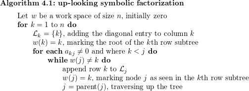
The up-looking symbolic factorization is based on the up-looking numeric factorization (4.1), in which the  $k$th row is computed from a triangular solve. The symbolic method constructs
 ${\mathcal{L}}$ one row
 $k$ at a time by traversing each row subtree (Davis Reference Davis2006). Selecting an entry
 $a_{kj}$ in the lower triangular part of
 $A$, Algorithm 4.1 walks up the elimination tree until it sees a marked node, and marks all nodes along the way. It will stop at the root
 $k$ since this starts out as marked. Each node seen in this traversal is one node of the
 $k$th row subtree. As a by-product, each
 ${\mathcal{L}}_{j}$ is in sorted order.
Rose et al. (Reference Rose, Tarjan and Lueker1976) present the first algorithm for computing  ${\mathcal{L}}$, using what could be seen as an abbreviated right-looking method. The downside of their method is that it requires a more complex dynamic data structure for
 ${\mathcal{L}}$ that takes more than
 $O(|L|)$ space. In their method, the sets
 ${\mathcal{L}}_{j}$ are initialized to the non-zero pattern of the lower triangular part of the matrix
 $A$ (that is,
 ${\mathcal{A}}_{j}\cup \{j\}$ from (4.3)). At each step
 $j$, duplicates in
 ${\mathcal{L}}_{j}$ are pruned, and then the set
 ${\mathcal{L}}_{j}$ is added to its parent in the elimination tree,
 $$\begin{eqnarray}{\mathcal{L}}_{\text{parent}(j)}={\mathcal{L}}_{\text{parent}(j)}\cup ({\mathcal{L}}_{j}\setminus \{j\}).\end{eqnarray}$$
As a result, by the time the  $j$th step starts, (4.3) has been computed for column
 $j$ since all the children of
 $j$ have been considered. Normally, computing the union of two sets takes time proportional to the size of the two sets, but the algorithm avoids this by allowing duplicates to temporarily reside in
 ${\mathcal{L}}_{\text{parent}(j)}$. Note that Rose et al. did not use the term ‘elimination tree’ since the term had not yet been introduced, but we use the term here since it provides a concise description of their method.
George and Liu (Reference George and Liu1980c) present the first linear-time symbolic factorization method using  $O(|L|)$ space, based on the path lemma and the quotient graph. To describe this method, we first need to consider two sub-optimal methods: one using only the graph of
 $A$, and the second using the elimination graph.
Recall that the path lemma states that  $l_{ij}\neq 0$ if and only there is a path in the graph of
 $A$ from
 $i$ to
 $j$ whose intermediate vertices are all numbered less than
 $\min (i,j)$ (that is, excluding
 $i$ and
 $j$ themselves). One method for constructing
 ${\mathcal{L}}_{j}$ is to apply the path lemma directly on
 $A$, and determine all nodes
 $i$ reachable from
 $j$ by traversing only nodes 1 to
 $j-1$ in the graph of
 $A$. This first alternative method based on the graph of
 $A$ would result in a compact data representation but would require a lot of work.
The second alternative is to mimic the outer-product factorization (4.2), by constructing a sequence of elimination graphs as in Algorithm 4.2 below. Let  $G_{0}$ be the graph of
 $A$ (with an edge
 $(i,j)$ if and only if
 $a_{ij}\neq 0$). Let
 $G_{j}$ be the graph of
 $A_{22}$ in (4.2) after the first
 $k$ nodes have been eliminated. Eliminating a node
 $j$ adds a clique to the graph between all neighbours of
 $j$.
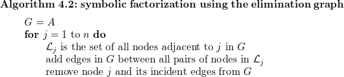
Algorithm 4.2 is not practical since it takes far too much time (the same time as the numeric factorization). However, Eisenstat, Schultz and Sherman (Reference Eisenstat, Schultz, Sherman, Bunch and Rose1976a) show how to represent the sequence of graphs in a more compact way, which George and Liu (Reference George and Liu1980c) refer to as the quotient graph. The quotient graph  ${\mathcal{G}}$ is a graph that contains two kinds of nodes: those corresponding to uneliminated nodes in
 $G$, and those corresponding to a subset of eliminated nodes in
 $G$. Each eliminated node
 $e$ results in a clique in
 $G$. If the eliminated node
 $e$ has
 $t$ neighbours, this requires
 $O(t^{2})$ new edges in
 $G$. Instead, we can create a new kind of node which George and Liu call a supernode. This is not quite the same as the term supernode used elsewhere in this article, so we will use Eisenstat et al.’s (Reference Eisenstat, Schultz, Sherman, Bunch and Rose1976a) term element to avoid confusion. The element
 $e$ represents the clique implicitly, with only
 $O(t)$ edges.
Algorithm 4.3 uses the notation of Amestoy, Davis and Duff (Reference Amestoy, Davis and Duff1996a). Let  ${\mathcal{A}}_{j}$ denote the (regular) nodes adjacent to
 $j$ in
 ${\mathcal{G}}$, and let
 ${\mathcal{E}}_{j}$ represent the elements adjacent to
 $j$. Finally, let
 ${\mathcal{L}}_{e}$ represent the regular nodes adjacent to element
 $e$; we use this notation because it is the same as the pattern of column
 $e$ of
 $L$. If one clique is contained within another, it can be deleted without changing the graph. As a result, no elements are adjacent to any other elements in the quotient graph.
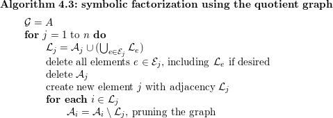
Edges are pruned from  ${\mathcal{A}}$ as Algorithm 4.3 progresses. Suppose there is an original edge
 $(i,k)$ between two nodes
 $i$ and
 $k$, but an element
 $j$ is formed that includes both of them. The two nodes are still adjacent in
 $G$ but this is represented by element
 $j$. The explicit edge
 $(i,k)$ is no longer needed. The quotient graph elimination process takes
 $O(|L|)$ time, and because edges are pruned and assuming
 ${\mathcal{L}}_{e}$ is deleted after it is used, Algorithm 4.3 only needs
 $O(|A|)$ memory. Keeping the pattern of
 $L$ requires
 $O(|L|)$ space.
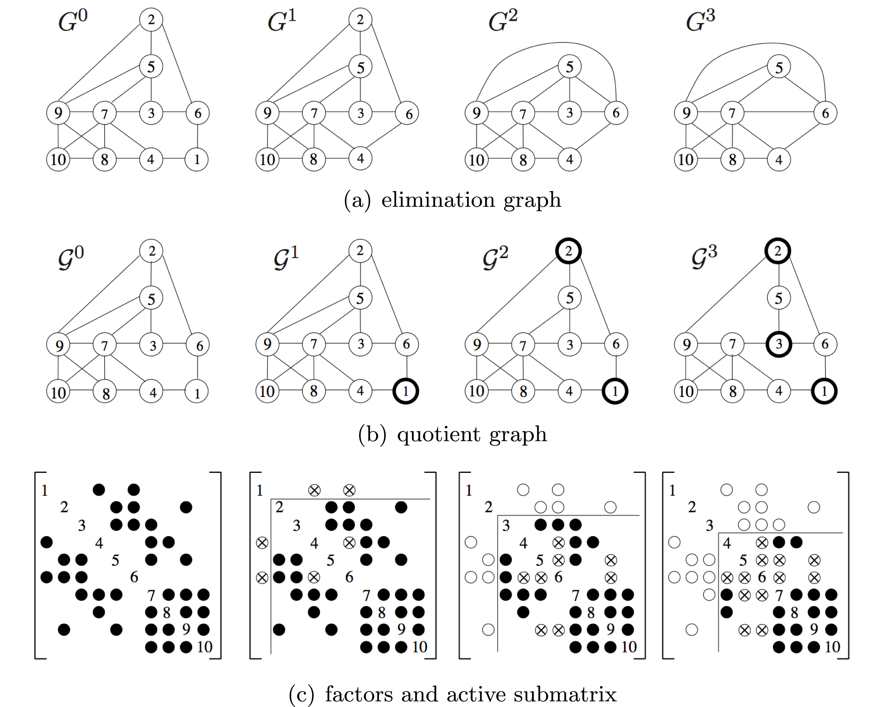
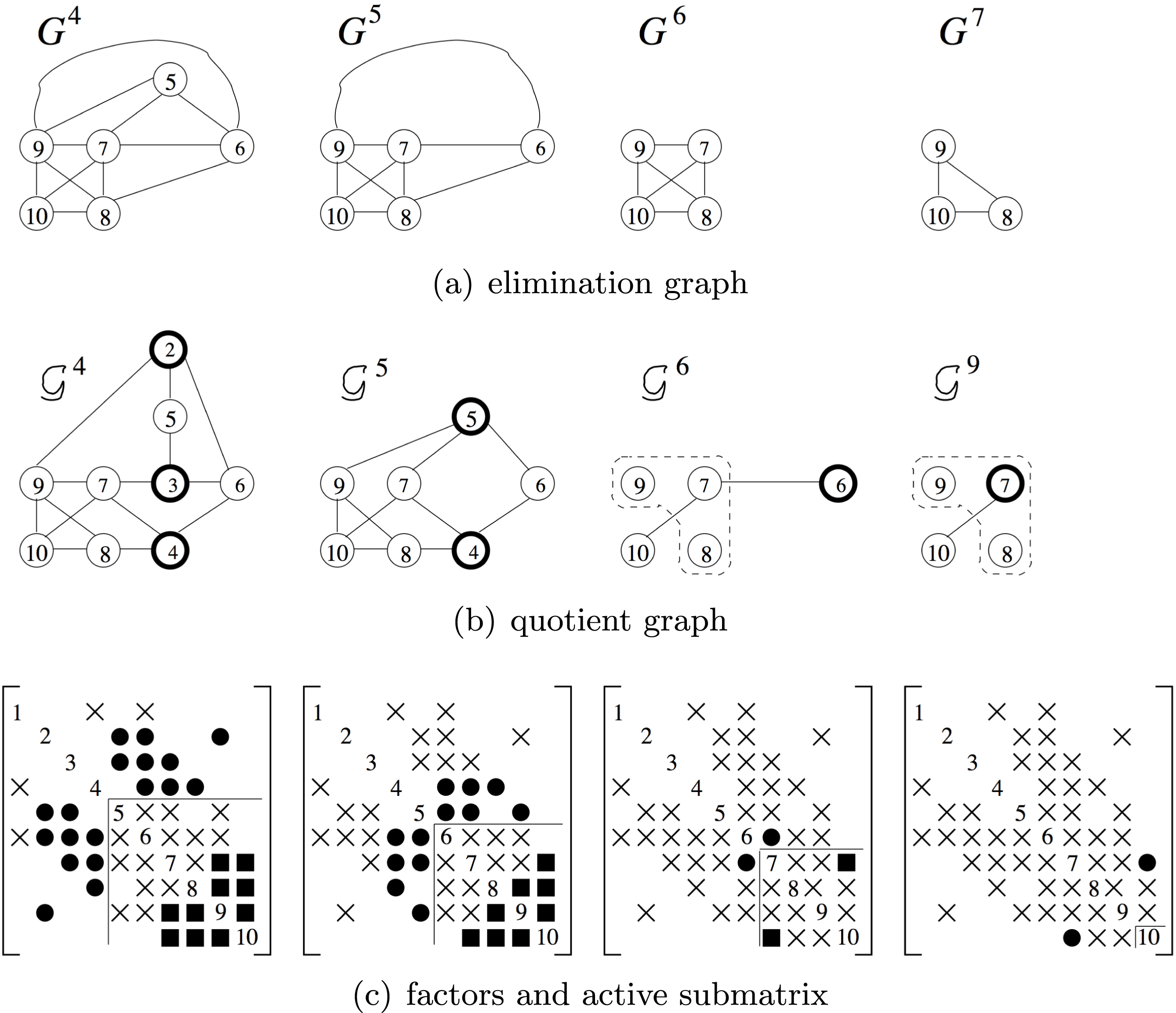
Figures 4.5 and 4.6 from Amestoy et al. (Reference Amestoy, Davis and Duff1996a) present the sequence of elimination graphs, quotient graphs, and the pattern of the factors after three steps of elimination. All three represent the same thing in different forms. In the graph  ${\mathcal{G}}_{2}$, element 2 represents a clique of nodes 5, 6, and 9, and thus the original edge (5,9) is redundant and has been pruned. In
 ${\mathcal{G}}_{5}$, element 5 is adjacent to prior elements 2 and 3, and thus the latter two elements are deleted.
Elimination graph, quotient graph, and matrix (Amestoy et al. Reference Amestoy, Davis and Duff1996a).
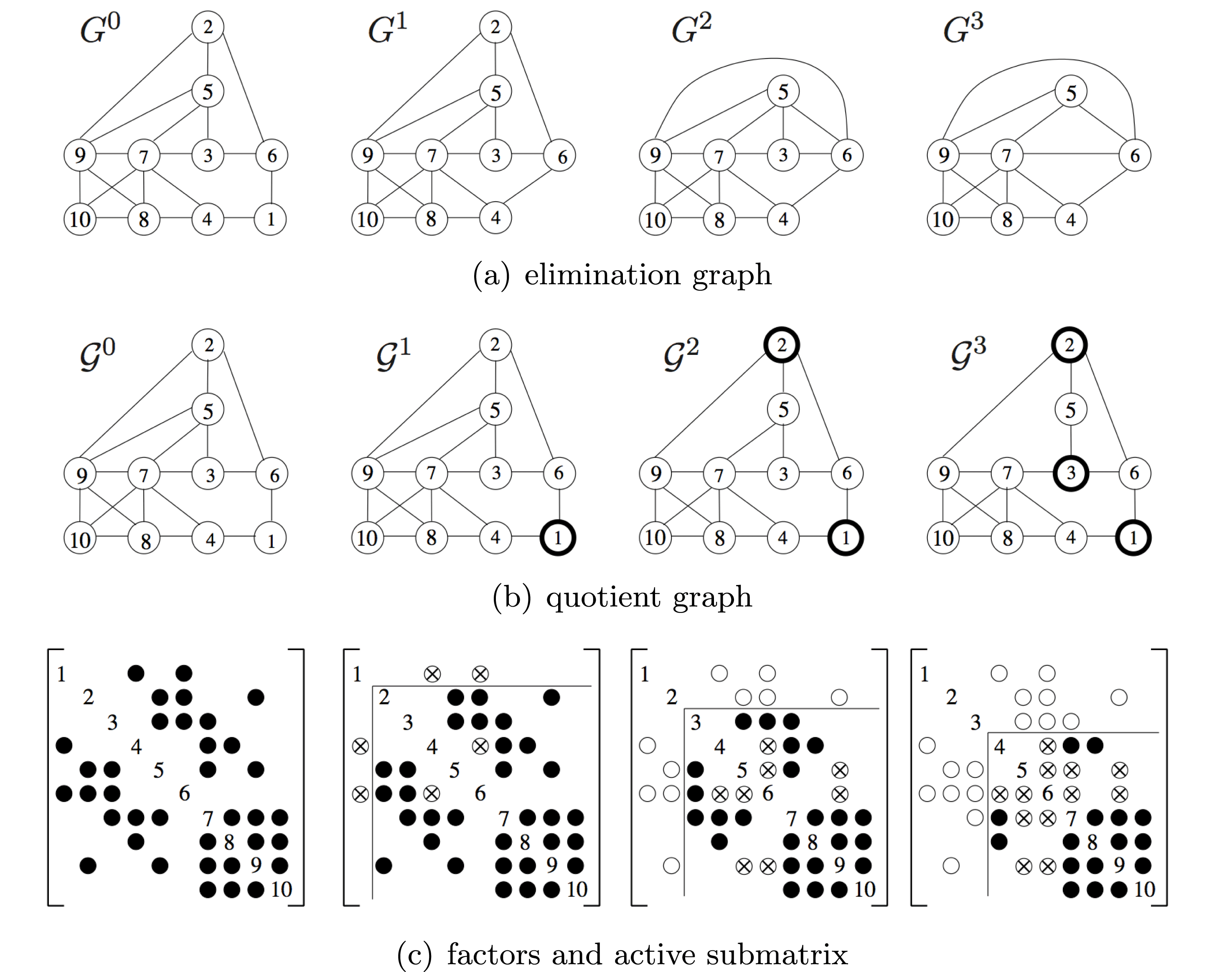
Elimination graph, quotient graph, and matrix (continued) (Amestoy et al. Reference Amestoy, Davis and Duff1996a).

Algorithm 4.3 takes  $O(|L|)$ time and memory to construct the non-zero pattern of
 $L$. Eisenstat, Schultz and Sherman (Reference Eisenstat, Schultz, Sherman, Bunch and Rose1976b) describe how the non-zero pattern of
 $L$ and
 $U$ can be represented in less space than one integer per non-zero entry. Suppose the matrix
 $L$ is stored by columns. If the non-zero pattern of a column
 $j$ of
 $U$ is identical to a subsequence of a prior row, then the explicit storage of the pattern of the
 $j$th column can be deleted, and replaced with a reference to the subsequence in the prior column. George and Liu (Reference George and Liu1980c) exploit this property to reduce the time and memory required for symbolic factorization, and extend it by relying on the elimination tree to determine when this property occurs. Suppose a node
 $j$ in the etree has a single child
 $c$, and that
 ${\mathcal{L}}_{j}={\mathcal{L}}_{c}\setminus \{c\}$. This is a frequently occurring special case of (4.3). If the etree is postordered,
 $c=j-1$ as well, further simplifying the representation. There is no need to store the pattern of
 ${\mathcal{L}}_{j}$ explicitly. If the row indices in
 ${\mathcal{L}}_{j-1}$ appear in sorted order, then
 ${\mathcal{L}}_{j}$ is the same list, excluding the first entry.
This observation can also be used to speed up the up-looking, left-looking, and right-looking symbolic factorization algorithms just described above. Each of them can be implemented in time and memory proportional to the size of the representation of the pattern of  $L$. The savings can be significant: for an
 $s\times s$ two-dimensional mesh using a nested dissection ordering, the matrix
 $A$ is
 $n\times n$ with
 $n=s^{2}$. The numeric factorization takes
 $O(s^{3})$ time and
 $|L|$ is
 $O(s^{2}\log s)$, but the compact representation of
 $L$ takes only
 $O(s^{2})$, or
 $O(n)$ space, and takes the same time to compute.
George, Poole and Voigt (Reference George, Poole and Voigt1978) and George and Rashwan (Reference George and Rashwan1980) extend the quotient graph model to combine nodes in the graph of  $A$ for the symbolic and numeric Cholesky factorization of a block partitioned matrix, motivated by the finite element method.
Gilbert (Reference Gilbert1994) surveys the use of graph algorithms for the symbolic analysis for Cholesky, QR, LU factorization, eigenvalue problems, and matrix multiplication. Most of his paper focuses on the use of directed graphs for non-symmetric problems, but many of the results he covers are closely related to the Cholesky factorization. For example, the Cholesky factorization of  $A^{T}A$ provides an upper bound for the non-zero pattern of QR and LU factorization of
 $A$. Pothen and Toledo (Reference Pothen, Toledo, Mehta and Sahni2004) give a more recent tutorial survey of algorithms and data structures for the symbolic analysis of both symmetric and unsymmetric factorizations. They discuss the elimination tree, skeleton graph, row/column counts, symbolic factorization (topics discussed above), and they also consider unsymmetric structures for LU and QR factorization.
Symbolic factorization algorithms take time proportional to the size of their output, which is often a condensed form of the pattern of  $L$ not much bigger than
 $O(|A|)$ itself. As a result, parallel speedup is very difficult to achieve. The practical goal of a parallel symbolic factorization algorithm is to exploit distributed memory to solve problems too large to fit on any one processor, which all of the following parallel algorithms achieve.
The first parallel algorithm to accomplish this goal was that of George, Heath, Ng and Liu (Reference George, Heath, Ng and Liu1987, Reference George, Heath, Liu and Ng1989a), which computes  ${\mathcal{L}}$ column-by-column in a distributed-memory environment. Their method assumes the elimination tree is already known, and obtains a very modest speedup. Ng (Reference Ng1993) extends this method by exploiting supernodes, which improves both sequential and parallel performance. Zmijewski and Gilbert (Reference Zmijewski and Gilbert1988) show how to compute the tree in parallel. The entries
 $A$ can be partitioned, and each processor computes its own elimination tree (forest, to be precise) on the entries it owns. These forests are then merged to construct the elimination tree of
 $A$. Once the elimination tree is known, their parallel symbolic factorization constructs the row subtrees of
 $L$, each one as an independent problem. They do not obtain any parallel speedup when computing the elimination tree, however. Likewise, Kumar et al. (Reference Kumar, Kumar and Basu1992) construct both the etree and
 ${\mathcal{L}}$ in parallel, and they obtain a modest parallel speedup in constructing the tree and in the symbolic factorization. Gilbert and Hafsteinsson (Reference Gilbert and Hafsteinsson1990) present a highly parallel shared-memory (CRCW) algorithm for finding the elimination tree and the pattern
 ${\mathcal{L}}$ using one processor for each entry in
 $L$, in
 $O(\log ^{2}n)$ time. They do not present an implementation, however.
Parallel symbolic factorization methods for LU factorization (Grigori, Demmel and Li Reference Grigori, Demmel and Li2007b), supernodal Cholesky (Ng Reference Ng1993), and multifrontal methods (Gupta, Karypis and Kumar Reference Gupta, Karypis and Kumar1997) are discussed in Sections 6.1, 9.1, and 11, respectively.
5 Cholesky factorization
This section presents some of the many variants of sparse Cholesky factorization. Sparse factorization methods come in two primary variants: (1) those that rely on dense matrix operations applied to the dense submatrices that arise during factorization, and (2) those that do not. Both of these variants exist in sequential and parallel forms, although most parallel algorithms also rely on dense matrix operations as well. The methods presented in this section do not rely on dense matrix operations: envelope and skyline methods (Section 5.1, which are now of only historical interest), the up-looking method (Section 5.2), the left-looking method (Section 5.3), and the right-looking method (Section 5.4). Supernodal, frontal, and multifrontal methods are discussed in Sections 9–11.
5.1 Envelope, skyline, and profile methods
Current algorithms exploit every zero entry in the factor, or nearly all of them, using the graph theory and algorithms discussed in Section 4. However, the earliest methods did not have access to these developments. Instead, they were only able to exploit the envelope. Using current terminology, the  $k$th row subtree
 ${\mathcal{T}}^{k}$ describes the non-zero pattern of the
 $k$th row of
 $L$ (refer to Figure 4.4). The leaves of this tree are entries in the skeleton matrix
 $\widehat{A}$, and the non-zero
 $a_{kj}$ with the smallest column index
 $j$ will always be the leftmost leaf. The
 $k$th row subtree will be a subset of nodes
 $j$ to
 $k$. That is, any non-zeros in the
 $k$th row of
 $L$ can only appear in columns
 $j$ to
 $k$. An algorithm that stores all of the entries
 $j$ to
 $k$ is called an envelope method. These methods are also referred to as profile or skyline methods (the latter is a reference to
 $L^{T}$).
Jennings (Reference Jennings1966) created the first envelope method for sparse Cholesky. Felippa (Reference Felippa1975) adapted the method for finite element problems by partitioning the matrix into two sets, according to internal degrees of freedom (those appearing only with a single finite element) and external degrees of freedom. Neither considered permutations to reduce the profile. While envelope/profile/skyline factorization methods are no longer commonly used, profile reduction orderings (Section 8.2) are still an active area of research since they are very well-suited to frontal methods (Section 10).
George and Liu (Reference George and Liu1978a, Reference George and Liu1978b, Reference George and Liu1979a) went beyond just two partitions in their recursive block partitioning method for irregular finite element problems. The diagonal block of each partition is factorized via an envelope method. They also consider ordering methods to find the partitions and to reduce the profiles of the diagonal blocks. The factorizations of the off-diagonal blocks are not stored, but computed column-by-column when needed in the forward/backsolves (George Reference George1974).
Bjorstad (Reference Bjorstad1987) uses a similar partitioned strategy, also exploiting parallelism by factorizing multiple partitions in parallel (each with a sequential profile method). Updates from each partition are applied in a right-looking manner and held on disk, similar to the strategy of George and Rashwan (Reference George and Rashwan1985), discussed in Section 5.3.
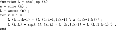
5.2 Up-looking Cholesky
Unlike the envelope method described in the previous section, the up-looking Cholesky factorization method presented here can exploit every zero entry in  $L$, and is asymptotically optimal in the work it performs. It computes each row of
 $L$, one at a time, starting with row 1 and proceeding to row
 $n$. The
 $k$th step requires a sparse triangular solve, with a sparse right-hand side, using the rows of
 $L$ already computed (
 $L_{1:k-1,1:k-1}$). It is also called the bordering method and row-Cholesky. It is not the first asymptotically optimal sparse Cholesky factorization algorithm, but it is presented first since it is closely related to presentation of the sparse triangular solve and symbolic analysis in Sections 3.2 and 4. It appears below in MATLAB.
Consider the up-looking factorization Algorithm 4.1 presented in Section 4.3. The algorithm traverses each disjoint subpath of the  $k$th row subtree,
 ${\mathcal{T}}^{k}$, but it does not traverse them in the topological order required for the numeric factorization, since this is not required for the symbolic factorization.
A simple change to the method results in a proper topological order that satisfies the numerical dependencies for the sparse triangular solve. Consider the computation of row 11 of  $L$, from Figure 4.4. Suppose the non-zeros of
 $A$ in columns 2, 3, 4, 8, and 10 are visited in that order (they can actually be visited in any order). The first disjoint path seen is
 $(2,4,10,11)$, from the first non-zero
 $a_{11,2}$ to the root of
 ${\mathcal{T}}^{11}$. These nodes are all marked. Next, the single node 3 is in a disjoint path by itself, since the path starts from the non-zero
 $a_{11,3}$ and halts when the marked node 4 is seen. Node 4 is considered because
 $a_{11,4}$ is non-zero, but node 4 is already marked so no path is formed. Node 8 gives the path
 $(8,9)$. Finally, node 10 is skipped because it is already marked.
The resulting disjoint paths are  $(2,4,10,11)$,
 $(3)$, and
 $(8,9)$, and are found in that order. These three paths cannot be traversed in that order for the triangular solve since (for example) the non-zero
 $l_{4,3}$ requires node 3 to appear before node 4. However, if these three paths are reversed, as
 $(8,9)$, then
 $(3)$, and finally
 $(2,4,10,11)$, we obtain a non-zero pattern for the sparse triangular solve as
 ${\mathcal{X}}=(8,9,3,2,4,10,11)$. This ordering of
 ${\mathcal{X}}$ is topological. If you consider any pair of nodes
 $j$ and
 $i$ in the list
 ${\mathcal{X}}$, then any edge in the graph
 $G_{L}$ (with an edge
 $(j,i)$ for each
 $l_{ij}\neq 0$) will go from left to right in that list. Performing the triangular solve from Section 3.2 in this order satisfies all numerical dependencies.
Sparse Cholesky factorization via the up-looking method was first considered by Rose, Whitten, Sherman and Tarjan (Reference Rose, Whitten, Sherman and Tarjan1980), but they did not provide an algorithm. Liu (Reference Liu1986a) introduces the row subtrees and the skeleton matrix as a method for a compact row-by-row storage scheme for  $L$. Each row subtree can be represented by only its leaves (each of which is an entry in the skeleton matrix). Liu did not describe a corresponding up-looking factorization method, however.
Bank and Smith (Reference Bank and Smith1987) describe an up-looking numeric factorization algorithm that is a companion to their up-looking symbolic factorization algorithm. They suggest two methods to handle the numerical dependencies in the triangular solve: (1) explicit sort, and (2) a traversal of the entries in each row of  $A$ in reverse order, which produces a topological order. This second method is optimal, and it appears to be the first instance of a topological ordering for a sparse triangular solve. However, to save space, they do not store the non-zero pattern of
 $L$. Instead, they construct each row or column as needed by traversing each row subtree. This reduces space but it leads to a non-optimal amount of work for their numeric factorization since it must rely on dot products of pairs of sparse vectors for the triangular solve. The computational cost of their method is analysed by Bank and Rose (Reference Bank and Rose1990).
Liu (Reference Liu1991) was the first to implement an asymptotically optimal up-looking method, via a generalization of the envelope method. The method partitions the matrix  $L$ into blocks. Each diagonal block corresponds to a chain of consecutive nodes in the elimination tree. That is, each chain consists of a sequence of
 $t$ columns
 $j,j+1,\ldots ,j+t$, where the parent of each column is the very next column in the sequence. The key observation is that the diagonal block
 $L_{j:j+t,j:j+t}$ has a full envelope, and the submatrix below this diagonal block, namely,
 $L_{j+t+1:n,j:j+t}$, also has a full envelope structure. In any given row
 $i$ of the subdiagonal block, if
 $l_{ik}$ is non-zero for some
 $k$ in the sequence
 $j,j+1,\ldots ,j+t$, then all entries in
 $L_{i,k:j+t}$ must also be non-zero. This is because each row subtree is composed of a set of disjoint paths, and the postordering of the elimination tree ensures that the subpaths consist of contiguous subsequences of the diagonal blocks.
Davis’s up-looking method (Reference Davis2005, Reference Davis2006) relies on a vanilla compressed-column data structure for  $L$, which also results in an asymptotically optimal amount of work.
Although the left-looking, supernodal, and multifrontal Cholesky factorizations are widely used and appear more frequently in the literature, the up-looking method is also widely used in practice. In particular, MATLAB relies on CHOLMOD for  and chol(A) when A is a sparse symmetric definite matrix (Chen, Davis, Hager and Rajamanickam Reference Chen, Davis, Hager and Rajamanickam2008). CHOLMOD’s symbolic analysis computes the row and column counts (Section 4.2), which also gives the floating-point work. If the ratio of the work over the number of non-zeros in
 $L$ is less than 40, CHOLMOD uses the up-looking method presented here, and a left-looking supernodal method otherwise (Section 9.1). This is because the up-looking method is fast in practice for very sparse matrices, as compared to supernodal and multifrontal methods.
5.3 Left-looking Cholesky
The left-looking Cholesky factorization algorithm is widely used and has been the focus of more research articles than the up-looking method. It is also called the fan-in or backward-looking method. It forms the foundation of the left-looking supernodal Cholesky factorization (Section 9.1). The method computes  $L$ one column at a time, and thus it is also called column-Cholesky. The method can be derived from the expression
 $$\begin{eqnarray}\left[\begin{array}{@{}ccc@{}}L_{11} & & \\ l_{12}^{T} & l_{22} & \\ L_{31} & l_{32} & L_{33}\end{array}\right]\left[\begin{array}{@{}ccc@{}}L_{11}^{T} & l_{12} & L_{31}^{T}\\ & l_{22} & l_{32}^{T}\\ & & L_{33}^{T}\end{array}\right]=\left[\begin{array}{@{}ccc@{}}A_{11} & a_{12} & A_{31}^{T}\\ a_{12}^{T} & a_{22} & a_{32}^{T}\\ A_{31} & a_{32} & A_{33}\end{array}\right]\!,\end{eqnarray}$$
where the middle row and column of each matrix are the  $k$th row and column of
 $L$,
 $L^{T}$, and
 $A$, respectively. If the first
 $k-1$ columns of
 $L$ are known, then the
 $k$th column of
 $L$ can be computed as follows:
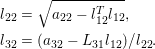 $$\begin{eqnarray}\begin{array}{@{}l@{}}l_{22}=\sqrt{a_{22}-l_{12}^{T}l_{12}},\\ l_{32}=(a_{32}-L_{31}l_{12})/l_{22}.\end{array}\end{eqnarray}$$
These two expressions can be folded together into a single operation, a sparse matrix times sparse vector, that computes a vector  $c$ of length
 $n-k+1$,
 $$\begin{eqnarray}c=\left[\begin{array}{@{}c@{}}c_{1}\\ c_{2}\end{array}\right]=\left[\begin{array}{@{}c@{}}a_{22}\\ a_{32}\end{array}\right]-\left[\begin{array}{@{}c@{}}l_{12}^{T}\\ L_{31}\end{array}\right]l_{12},\end{eqnarray}$$
where  $c_{1}$ and
 $a_{22}$ are scalars, and
 $c_{2}$ and
 $a_{32}$ are vectors of size
 $n-k$. Computing
 $c$ is the bulk of the work for step
 $k$ of the algorithm; this is followed by
 $$\begin{eqnarray}\displaystyle l_{22} & \displaystyle =\sqrt{c_{1}}, & \displaystyle \\ \displaystyle l_{32} & \displaystyle =c_{2}/l_{22}.\end{eqnarray}$$
The MATLAB equivalent is given below.
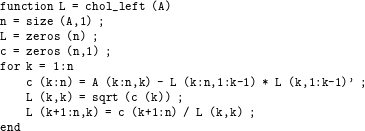
The key observation is that this sparse matrix times sparse vector multiply (5.3) needs to be done only for columns for which  $l_{12}^{T}$ is non-zero, which corresponds to a traversal of each node in the
 $k$th row subtree,
 ${\mathcal{T}}^{k}$. In MATLAB notation the computation of c(k:n) is then as follows.

In Algorithm 5.1 below,  $L$ is stored in compressed-column form. It requires access to the
 $k$th row of
 $L$, or
 $l_{12}^{T}$ in (5.3) at the
 $k$ step. Accessing an arbitrary row in this data structure would take too much time, but fortunately the access to the rows of
 $L$ is not arbitrary. Rather, the algorithm requires access to each row in a strictly ascending order. To accomplish this, the left-looking algorithm keeps track of a pointer into each column that advances to the next row as each row is accessed (the workspace
 $p$).

The algorithm traverses  ${\mathcal{T}}^{k}$ the same way as the
 $k$th iteration of Algorithm 4.1, so the details are not given here. The cmod and cdiv operations defined in Algorithm 5.1 are discussed below.
Rose et al. (Reference Rose, Whitten, Sherman and Tarjan1980) give an overview of three sparse Cholesky methods (right-looking, up-looking, and left-looking), and ordering methods. The left-looking method they consider is YSMP, by Eisenstat et al. (Reference Eisenstat, Schultz and Sherman1975, Reference Eisenstat, Gursky, Schultz and Sherman1982, Reference Eisenstat, Schultz and Sherman1981). YSMP is actually described as computing  $L^{T}$ one row at a time, which is equivalent to the left-looking column-by-column method in Algorithm 5.1 above. SPARSPAK is also based on the left-looking sparse Cholesky algorithm (Chu, George, Liu and Ng Reference Chu, George, Liu and Ng1984, George and Liu Reference George and Liu1981, George and Ng Reference George and Ng1985a, George and Ng Reference George and Ng1984b).
YSMP and SPARSPAK both rely on a set of  $n$ dynamic linked lists to traverse the row subtrees, one for each row. Each column
 $j$ is in only a single linked list at a time. In Algorithm 5.1,
 $p_{j}$ refers to the location in column
 $j$ of the next entry that will be accessed. If the entry has row index
 $t$, then column
 $j$ will reside in list
 $t$. When
 $p_{j}$ advances, column
 $j$ is moved to the linked list for the next row. As a result, when step
 $k$ commences, the
 $k$th linked list contains all nodes in the
 $k$th row subtree,
 ${\mathcal{T}}^{k}$.
The left-looking sparse Cholesky algorithm has been the basis of many parallel algorithms for both shared-memory and distributed-memory parallel computers. It is easier to exploit parallelism in this method as compared to the up-looking method.
The elimination tree plays a vital role in all parallel sparse direct methods. Different methods (e.g. left-looking, right-looking, supernodal, multifrontal) define their tasks in many different ways, but in all the methods the tree governs the parallelism. In some methods, each node of the tree is a single task, but more often, the work at a given node is split into multiple tasks. Tasks on independent branches of the tree can be computed in parallel.
George, Heath, Liu and Ng (Reference George, Heath, Liu and Ng1986a) present the first parallel left-looking sparse Cholesky method, using a shared-memory computer. Algorithm 5.1 contains two basic tasks, each of which operate on the granularity of one or two columns: (1) cmod( $k,j$), the modification of column
 $k$ by column
 $j$, and (2) cdiv(
 $k$), the division of column
 $k$ by the diagonal,
 $l_{kk}$. Their parallel version of Algorithm 5.1 uses the same linked list structure as their sequential method, and one independent task per column
 $k$. Task
 $k$ waits until a column
 $j$ appears in the
 $k$th link list, and then performs the cmod(
 $k,j$) and moves the column
 $j$ to the next linked list (incrementing
 $p_{j}$). When all nodes in row
 $k$ have been processed, task
 $k$ finishes by performing the cdiv(
 $k$) task. Only task
 $k$ needs write-access to column
 $k$. Each node of the elimination tree defines a single task. In their method, a task can overlap with other tasks below it and above it in the tree, but a column
 $j$ can only modify one ancestor column
 $k$ at a time. As an example, consider the matrix and tree in Figure 4.3. Suppose columns 2 and 4 have been computed (tasks 2 and 4 are done), and cmod(10,2) has been completed by task 10, which then places column 2 in the list for task 11. Then task 10 can do cmod(10,4) at the same time task 11 does cmod(11,2). However, tasks 10 and 11 cannot do cmod(10,2) and cmod(11,2), respectively, at the same time; task 11 must wait until task 10 finishes cmod(10,2) before it can use column 2 for cmod(11,2).
Liu (Reference Liu1986b) considers three models for sparse Cholesky: fine-, medium-, and coarse-grained, placing them in a common framework. The fine-grained model considers each floating-point operation as its own task; see for example the LU factorization method by Wing and Huang (Reference Wing and Huang1980). The coarse-grained model is exemplified by Jess and Kees (Reference Jess and Kees1982), who propose a parallel right-looking LU factorization for matrices with symmetric structure (the methods of Wing and Huang (Reference Wing and Huang1980) and Jess and Kees (Reference Jess and Kees1982) are discussed in Section 6.3, on the right-looking LU factorization). The medium-grained model introduced by Liu (Reference Liu1986b) considers each cmod and cdiv as its own task. Each node of the  $n$ nodes in Liu’s graph is a cdiv, and each edge corresponds to a cmod, and thus the graph has same structure as
 ${\mathcal{L}}$, with
 $|{\mathcal{L}}|$ tasks. Task cmod(
 $k,j$) for any non-zero
 $l_{kj}$ in row
 $k$ must precede cdiv(
 $k$), which in turn must precede cmod(
 $i,k$) for any non-zero
 $l_{ik}$ in column
 $k$. Using the same example of Figure 4.3, in this model cmod(10,2) and cmod(11,2) can be done in parallel. Coalescing the tasks cdiv(
 $k$) with all tasks cmod(
 $i,k$) for each non-zero
 $l_{ik}$ in column
 $k$ results in the coarse-grained right-looking Cholesky, whereas combining all cmod(
 $k,j$) for each
 $l_{kj}$ in row
 $k$, with cdiv(
 $k$), results in a parallel left-looking Cholesky method.
Once the left-looking factorization progresses to step  $k$, it no longer needs the first
 $k-1$ rows of
 $L$ (the
 $L_{11}$) matrix. George and Rashwan (Reference George and Rashwan1985) exploit this property in their out-of-core method. They partition the matrix with incomplete nested dissection. Submatrices are factorized with a left-looking method, and then the remainder of the unfactorized matrix is updated (a right-looking phase) and written to disk. It is read back in when subsequent submatrices are factorized. Liu (Reference Liu1987a) also exploits this property in his out-of-core method. Unlike George and Rashwan’s (Reference George and Rashwan1985) method, Liu’s method is purely left-looking. The columns of
 $L$ are computed one at a time, and the memory space required grows as a result. If memory is exhausted, the
 $L_{11}$ matrix is written to disk, and the factorization continues. The
 $L_{21}$ matrix (rows
 $k$ to
 $n$) remains in core. To improve memory usage, the matrix is permuted via a generalization of the pebble game, applied to the elimination tree (Liu Reference Liu1987b).
George, Heath, Liu and Ng (Reference George, Heath, Liu and Ng1988a) extend their parallel left-looking method to the distributed-memory realm, where no processors share any memory and all data must be explicitly communicated by sending and receiving messages. Using the nomenclature of Ashcraft, Eisenstat, Liu and Sherman (Reference Ashcraft, Eisenstat, Liu and Sherman1990b), the method becomes right-looking, and so it is considered in Section 5.4.
If  $l_{ij}$ is non-zero, then at some point column
 $j$ must update column
 $i$, via cmod(
 $i,j$). In a left-looking method, the update from column
 $j$ to column
 $i$ (cmod(
 $i,j$)) is done at step
 $i$, according to the target column. In a right-looking method, cmod(
 $i,j$) is done at step
 $j$, according to the source column. The difference between left/right-looking in a parallel context is subtle, because it depends on where you are standing and which processor is being considered: the one sending an update or the one receiving it. Multiple steps can execute in parallel, although numerical dependencies must be followed. That is, if
 $l_{ij}$ is non-zero, then column
 $i$ must be finalized before cmod(
 $i,j$) can be computed.
Ashcraft, Eisenstat and Liu (Reference Ashcraft, Eisenstat and Liu1990a) observe that the method of George et al. (Reference George, Heath, Liu and Ng1989a) sends more messages than necessary. Suppose that one processor A owns both columns  $k_{1}$ and
 $k_{2}$, and both columns need to update a target column
 $i$ owned by a second processor B. In George et al.’s (Reference George, Heath, Liu and Ng1989a) method processor A sends two messages to processor B – column
 $k_{1}$ and column
 $k_{2}$ – so that processor B can compute cmod(
 $i,k_{1}$) and cmod(
 $i,k_{2}$). In the left-looking (fan-in) method of Ashcraft et al. (Reference Ashcraft, Eisenstat and Liu1990a), the update (5.3) for these two columns of
 $L$ is combined by processor A, which then sends only a single column to processor B, as an aggregated update. Constructing aggregate updates takes extra memory, and if this is not available, Eswar, Huang and Sadayappan (Reference Eswar, Huang and Sadayappan1994) describe a left-looking method that delays the construction of the update until other aggregate updates have been computed, sent, and freed.
All of the parallel methods described so far assign one or more entire columns of  $L$ to a single processor, resulting in a one-dimensional assignment of tasks to processors (columns only). Schreiber (Reference Schreiber, George, Gilbert and Liu1993) shows that any one-dimensional mapping is inherently non-scalable because of communication overhead, and that a two-dimensional mapping of computations to processors is required instead (Gilbert and Schreiber Reference Gilbert and Schreiber1992). These mappings are possible in supernodal and multifrontal methods, discussed in Sections 9 and 11, and in a two-dimensional right-looking method considered in the next section.
5.4 Right-looking Cholesky
Right-looking Cholesky, also known as fan-out or submatrix-Cholesky, is based on equation (4.2). It is described as follows in MATLAB notation as chol_right.
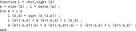
At step  $k$, the outer product L(k+1:n,k)*L(k+1:n,k)’ is subtracted from the lower right
 $(n-k)\times (n-k)$ submatrix. This is difficult to implement since it can take extra work to find the entries in
 $A$ to modify. There are many target columns, and any given target column may have many non-zeros that are not modified by the
 $k$th update. This is not a concern in the left- or up-looking methods, since in those methods the single target column is temporarily held in a work vector of size
 $n$, accessed via gather/scatter.
George et al. (Reference George, Heath, Liu and Ng1988a) present a parallel right-looking method for a distributed-memory computer. Each processor owns a set of columns. Any column  $k$ with no non-zeros in row
 $k$ of
 $L$ can be processed immediately via cdiv(
 $k$); this node
 $k$ is a leaf of the elimination tree. After a processor owning column
 $k$ does its cdiv(
 $k$), it sends column
 $k$ of
 $L$ to any processor owning any column
 $i$ for which
 $l_{ik}$ is non-zero. If a receiving processor owns more than one such column
 $i$, the message is sent only once. When a processor receives a column
 $j$, it computes cmod(
 $k,j$) for any column
 $k$ it owns. This is also a right-looking view, since a single column
 $j$ is applied to the submatrix of all columns owned by this processor. If given a single processor, the method is identical to the right-looking method, since one processor owns the entire matrix. When all cmods have been applied to a column
 $k$ that it owns, it does cdiv(
 $k$) and sends it out, as just described. Column tasks correspond to each node of the elimination tree, and are assigned to processors in a simple wrap-around manner. That is, the leaves are all doled out to processors in a round-robin manner, followed by all nodes one level up from the levels, and so on to the root.
George et al. (Reference George, Heath, Liu and Ng1989a) extend their method to the hypercube. They change the task assignment so that whole subtrees of the elimination tree are given to individual processors. In this case, the subtree is a node  $k$ and all its descendants, not to be confused with the
 $k$th row subtree,
 ${\mathcal{T}}^{k}$. They also show that performance can be improved via pipelining. When a processor receives a column
 $j$, it does all cmod(
 $k,j$) for all columns
 $k$ that it owns. However, rather than waiting until all such cmod(
 $k,j$)s are finished, it finalizes any column
 $k$ that is now ready for its cdiv(
 $k$) and sends it out, before continuing with the rest of the cmods for this incoming column
 $j$. George, Liu and Ng (Reference George, Liu and Ng1989b) analyse the communication between processors in this method and show that it is asymptotically optimal for a two-dimensional mesh with the nested dissection ordering. Gao and Parlett (Reference Gao and Parlett1990) augment the analysis of George et al. (Reference George, Liu and Ng1989b), showing that not only is the total communication volume minimized, but it is also balanced across the processors.
Ordering methods such as minimum degree can generate unbalanced trees. Geist and Ng (Reference Geist and Ng1989) generalize the subtree-to-subcube task assignment of George et al.’s (Reference George, Heath, Liu and Ng1989a) method via a bin-packing to account for heavily unbalanced trees. Eswar, Huang and Sadayappan (Reference Eswar, Huang and Sadayappan1995) consider task assignments that combine multiple strategies (wrap-based and subtree-based) for mapping processors to columns.
Zhang and Elman (Reference Zhang and Elman1992) explore several shared-memory variants: the left-looking methods of George et al. (Reference George, Heath, Liu and Ng1986a) and Ashcraft et al. (Reference Ashcraft, Eisenstat and Liu1990a), and the task-scheduling method of Geist and Ng (Reference Geist and Ng1989). The latter two are distributed-memory algorithms. Zhang and Elman report that Geist and Ng’s (Reference Geist and Ng1989) method works well in a shared-memory environment.
Ashcraft et al. (Reference Ashcraft, Eisenstat, Liu and Sherman1990b) and Eswar, Sadayappan and Visvanathan (Reference Eswar, Sadayappan, Visvanathan, Özgüner and Erçal1993a) both observe that the right-looking method of Geist and Ng (Reference Geist and Ng1989) sends more messages than both the distributed multifrontal method and the left-looking method with aggregated updates.
Jess and Kees (Reference Jess and Kees1982) describe a parallel right-looking LU factorization method for matrices with symmetric non-zero pattern, and with no pivoting, so their method can also be viewed as a way to compute the right-looking Cholesky factorization. Each node  $k$ of the elimination tree corresponds to cdiv(
 $k$) followed by cmod(
 $i,k$) for all non-zeros
 $l_{ik}$. The tree describes the parallelism, since nodes that do not have an ancestor/descendant relationship can be computed in parallel. This assumes that multiple updates to the same column are handled correctly. The updates cmod(
 $i,k_{1}$) and cmod(
 $i,k_{2}$) can be computed in any order, but a race condition could occur if two processes attempt to update the same target column
 $i$ at the same time. Jess and Kees (Reference Jess and Kees1982) use a critical-path scheduling strategy, with the simplifying assumption that each node takes the same amount of time to compute.
Manne and Haffsteinsson (Reference Manne and Haffsteinsson1995) describe a right-looking method for a SIMD parallel computer with a two-dimensional processor mesh. In a SIMD machine, all processors perform the same operation in lock-step fashion. With the correct mapping scheme, this strategy simplifies the synchronization between processors, so that the problem of simultaneous updates to the same entry is resolved. They rely on a two-dimensional mapping scheme that assigns all entries in a column of  $L$ to one column of processors and all entries in a row of
 $L$ to a single row of processors. The same mapping is used for both rows and columns. Thus,
 $a_{ij}$ is given to the processor in row
 $M(i)$ and column
 $M(j)$ of the two-dimensional processor mesh. Since each entry is owned by a single processor, multiple updates to the same entry are done in successive steps. Each outer loop of the chol_right algorithm above is done sequentially. Within the
 $k$th iteration, each processor iterates over the cmod operations it must compute. Note that a single processor only does part of any given cmod, since it does not own an entire column of the matrix.
Aggregating updates and sending a single message instead of one message is a common theme for many algorithms presented here. Ashcraft et al. (Reference Ashcraft, Eisenstat and Liu1990a) use this strategy for the left-looking method. The multifrontal method handles the submatrix update in an entirely different manner by delaying the updates and aggregating them. Hulbert and Zmijewski (Reference Hulbert and Zmijewski1991) consider a non-multifrontal right-looking method that also aggregates messages. Their method is based on the hypercube algorithm of George et al. (Reference George, Heath, Liu and Ng1989a) and Geist and Ng (Reference Geist and Ng1989). After a processor computes cdiv( $k$) for a column
 $k$ that it owns, cmod(
 $j,k$) must be computed for each non-zero
 $l_{jk}$ in column
 $k$. Some of these will be owned by the same processor, and these computations can be done right away. Others columns are owned by other processors. The method of George et al. (Reference George, Heath, Liu and Ng1989a) and Geist and Ng (Reference Geist and Ng1989) would send column
 $k$ to those other processors right away. Hulbert and Zmijewski (Reference Hulbert and Zmijewski1991) take another approach. The algorithm operates in two distinct phases. In the first phase, the method places column
 $k$ in an outgoing message queue, waits until all local computations that can be completed have finished. The queue acquires multiple messages for any given target processor. If there are multiple messages from this processor to the same target column, these are summed into a single aggregate column update (just as in the left-looking method of Ashcraft et al. Reference Ashcraft, Eisenstat and Liu1990a). As soon as the process runs out of local work it enters the second phase, which is identical to the original method of George et al. (Reference George, Heath, Liu and Ng1989a) and Geist and Ng (Reference Geist and Ng1989). In the second phase, the outgoing message queue is no longer used, and updates are sent as soon as they are computed. Hulbert and Zmijewski (Reference Hulbert and Zmijewski1991) show that this strategy results in a significant reduction in message traffic.
Ashcraft (Reference Ashcraft, George, Gilbert and Liu1993) generalizes the notion of left/right-looking and fan-in/out. Each non-zero  $l_{ij}$ defines a cmod(
 $i,j$). Recall that in the left-looking/fan-in method, cmod(
 $i,j$) is done at step
 $i$ and in a right-looking/fan-out method, cmod(
 $i,j$) is done at step
 $j$. There is no reason to use all one method or the other; each cmod(
 $i,j$) can be individually assigned to task
 $i$ or task
 $j$. In Ashcraft’s (Reference Ashcraft, George, Gilbert and Liu1993) fan-both method the processors are aligned in a two-dimensional grid. The processor grid tiles the matrix, and if a processor owns the diagonal entry
 $l_{kk}$, then it owns column
 $k$. If it also owns
 $l_{kj}$, then cmod(
 $k,j$) is treated in a left-looking (fan-in) fashion, and if it owns
 $l_{ik}$, then cmod(
 $j,k$) is treated in a right-looking (fan-out) fashion.
We consider parallel supernodal, frontal, and multifrontal Cholesky factorization methods in Sections 9–11.
6 LU factorization
LU factorization is most often used for square unsymmetric matrices when solving  $Ax=b$. It factors a matrix
 $A$ into the product
 $A=LU$, where
 $L$ is lower triangular and
 $U$ is upper triangular. Historically, the most common method for dense matrices is a right-looking one (Gaussian elimination); both it and a left-looking method are presented here. Section 6.1 considers the symbolic analysis phase for LU factorization, and its relationship with symbolic Cholesky and QR factorization. The next three sections present the left-looking method (Section 6.2) and two variants of the right-looking method (Sections 6.3 and 6.4). The first variant relies on a static data structure with some or all pivot choices made prior to numeric factorization, and the second variant relies on a dynamic data structure and finds its pivots during numeric factorization.
6.1 Symbolic analysis for LU factorization
If  $A$ is square and symmetric, and no numerical pivoting is required, then the non-zero pattern of
 $L+U$ is the same as the Cholesky factorization of
 $A$. This observation provides the framework for several LU factorization algorithms presented here. Other methods consider the symbolic analysis of a matrix with unsymmetric structure, but with no pivoting. If arbitrary row interchanges can occur due to partial pivoting, then LU factorization is more closely related to QR factorization, a fact that other methods rely on. Both strategies are discussed immediately below, in this section. Other methods allow for arbitrary row and column pivoting during numeric factorization, and for such methods a prior symbolic analysis is not possible at all. Many of the results in this section for sparse LU (and also QR factorization) are surveyed by Gilbert and Ng (Reference Gilbert, Ng, George, Gilbert and Liu1993) and Gilbert (Reference Gilbert1994). Pothen and Toledo (Reference Pothen, Toledo, Mehta and Sahni2004) consider both the symmetric and unsymmetric cases in their recent survey of graph models of sparse elimination.
6.1.1 Symbolic LU factorization without pivoting
Rose and Tarjan (Reference Rose and Tarjan1978) were the first to methodically consider the symbolic structure of Gaussian elimination for unsymmetric matrices. They model the matrix as a directed graph where edge  $(i,j)$ corresponds to the non-zero
 $a_{ij}$. They extend their path lemma for symmetric matrices (Rose et al. Reference Rose, Tarjan and Lueker1976) to the unsymmetric case. In the directed graph
 $G_{L+U}$ of
 $L+U$,
 $(i,j)$ is an edge (a non-zero in either
 $L$ or
 $U$, depending on where it is), if and only if there is a path in the directed graph of
 $A$ whose intermediate vertices are numbered less than
 $i$ and
 $j$ (excluding the endpoints
 $i$ and
 $j$ themselves). They present a symbolic factorization that uses this theorem to construct the pattern of
 $L$ and
 $U$ (a generalization of their symmetric method in Rose et al. Reference Rose, Tarjan and Lueker1976). The method is costly, taking the same time as the numeric factorization. These results and algorithm are also not general since they do not consider numerical pivoting during numeric factorization, which is often essential.
Eisenstat and Liu (Reference Eisenstat and Liu1992) show how symmetry can greatly reduce the time complexity of symbolic factorization. For each  $j$, let
 $k$ be the first off-diagonal entry that appears in both the
 $j$th row of
 $U$ and the
 $j$th column of
 $L$ (
 $\text{FSNZ}(j)=\min \{k|l_{kj}u_{jk}\neq 0\}$, the first symmetric non-zero), assuming such an entry exists. Entries beyond this first symmetric pair can be ignored in
 $L$ and
 $U$ when computing fill-in for subsequent rows and columns of
 $L$ and
 $U$. If applied to a symmetric matrix, the first symmetric pair occurs immediately, and is simply the parent of
 $j$ in the elimination tree. In this case, the method reduces to a Cholesky symbolic factorization, and the time is
 $O(|L|+|U|)$. The algorithm was implemented in YSMP (Eisenstat, Gursky, Schultz and Sherman Reference Eisenstat, Gursky, Schultz and Sherman1977) but not described at that time. Eisenstat and Liu (Reference Eisenstat and Liu1992) generalize this symmetric pruning to a path-symmetric reduction, where
 $s$ is the smallest node for which a path
 $j{\rightsquigarrow}k$ exists in both the graph of
 $L$ and
 $U$. Entries beyond
 $s$ in
 $L$ and
 $U$ can be ignored, and since
 $s\leq \text{FSNZ}(j)$, this can result in further pruning.
The quotient graph was first used by George and Liu (Reference George and Liu1980c) to represent the lower right  $(n-k)\times (n-k)$ active submatrix in a symbolic right-looking factorization (a Schur complement), after
 $k$ steps of elimination. Eisenstat and Liu (Reference Eisenstat, Liu, George, Gilbert and Liu1993b) generalize this representation for the unsymmetric case, and provide a catalogue of many different approaches with varying degrees of compression and levels of work to construct and maintain the representation. The edge
 $(i,j)$ in the Schur complement is present if and only if there is a path from
 $i$ to
 $j$ whose intermediate vertices are in the range 1 to
 $k$. Strongly connected components amongst nodes 1 to
 $k$ can be merged into single nodes, and the paths are still preserved. They also characterize a skeleton matrix for the unsymmetric case, whose filled graph is the same as the original matrix.
6.1.2 Symbolic LU with pivoting and its relationship to QR factorization
Consider both  $LU=PA$ and
 $QR=A$, where
 $P$ is determined by partial pivoting. George and Ng (Reference George and Ng1985b, Reference George and Ng1987) have shown that
 $R$ is an upper bound on the pattern of
 $U$. More precisely,
 $u_{ij}$ can be non-zero if and only if
 $r_{ij}\neq 0$. Gilbert and Ng (Reference Gilbert, Ng, George, Gilbert and Liu1993) and Gilbert and Grigori (Reference Gilbert and Grigori2003) strengthened this result, showing that the bound is tight if
 $A$ is strong-Hall. A matrix is strong-Hall if it cannot be permuted into block upper triangular form with more than one block (Section 8.7.3). This upper bound is tight in a one-at-a-time sense; for any
 $r_{ij}\neq 0$, there exists an assignment of numerical values to entries in the pattern of
 $A$ that makes
 $u_{ij}\neq 0$. The outline of the proof can be seen by comparing Gaussian elimination with Householder reflections. Additional details are given in the qr_right_householder function discussed in Section 7.
Both LU and QR factorization methods eliminate entries below the diagonal. For a Householder reflection, George, Liu and Ng (Reference George, Liu and Ng1988b) show that the non-zero pattern of all rows affected by the transformation take on a non-zero pattern that is the union of all of these rows. With partial pivoting and row interchanges, these rows are candidate pivot rows for LU factorization. Only one of them is selected as the pivot row. Every other candidate pivot row is modified by adding to it a scaled copy of the pivot row. Thus, an upper bound on the pivot row pattern is the union of all candidate pivot rows. This also establishes a bound on  $L$, namely, the non-zero pattern of
 $V$, which is a matrix whose column vectors correspond to the Householder reflections used for QR factorization.
With this relationship, a symbolic QR ordering and analysis (Section 7.1) becomes one possible symbolic ordering and analysis method for LU factorization. It is also possible to statically preallocate space for  $L$ and
 $U$. The bound can be loose, however. In particular, if the matrix is diagonally dominant, then no pivoting is needed to maintain numerical accuracy. This is called static pivoting, where all pivoting is done prior to numeric factorization. If the matrix
 $A$ also has a symmetric non-zero pattern (or if all entries in the pattern of
 $A+A^{T}$ are considered to be ‘non-zero’), then the non-zero patterns of
 $L$ and
 $U$ are identical to the pattern of the Cholesky factors
 $L$ and
 $L^{T}$, respectively, of a symmetric positive definite matrix with the same non-zero pattern as
 $A+A^{T}$. In this case, a symmetric fill-reducing ordering of
 $A+A^{T}$ is appropriate. Alternatively, the permutation matrix
 $Q$ can be selected to reduce the worst-case fill-in for
 $PAQ=LU$ for any
 $P$, and then the permutation
 $P$ can be selected solely on the basis of partial pivoting, with no regard for sparsity.
Thus, LU factorization can rely on three basic strategies for finding a fill-reducing ordering. Two of them are methods used prior to factorization: (1) a symmetric pre-ordering of  $A+A^{T}$, and (2) a column pre-ordering suitable for QR factorization. These options are discussed in Section 8. The third option is to dynamically choose pivots during numeric factorization, as discussed in Section 6.4.
With the QR upper bound, LU factorization can proceed using a statically allocated memory space. This bound can be quite high, however. It is sometimes better just to make a guess at the final  $|L|$ and
 $|U|$, or to guess that no partial pivoting will be needed and to use a symbolic Cholesky analysis to determine a guess for
 $|L|$ and
 $|U|$. Sometimes a good guess is available from the LU factorization of a similar matrix in the same application. The only penalty for making a wrong guess is that the memory space for
 $|L|$ or
 $|U|$ must be reallocated if the guess is too low, or memory may run out if the guess is too high.
In contrast to Rose and Tarjan (Reference Rose and Tarjan1978) and Eisenstat and Liu (Reference Eisenstat and Liu1992), George and Ng (Reference George and Ng1987) consider partial pivoting. They rely on their result that QR forms an upper bound for LU to create a symbolic factorization method for both QR and LU. The resulting non-zero patterns for  $L$ and
 $U$ can accommodate any partial pivoting with row interchanges. The symbolic factorization takes
 $O(|L|+|U|)$ time, which is much faster than Rose and Tarjan’s (Reference Rose and Tarjan1978) method. Their method (Algorithm 6.1 below) is much like the row-merge QR factorization of George and Heath (Reference George and Heath1980), which we discuss in Section 7.2. In this algorithm,
 ${\mathcal{L}}_{k}$ is set of row indices that is the upper bound on the pattern of the
 $k$th column of
 $L$,
 ${\mathcal{U}}_{k}$ is the upper bound on the
 $k$th row of
 $U$, and
 ${\mathcal{A}}_{i}$ is the pattern of the
 $i$th row of
 $A$.
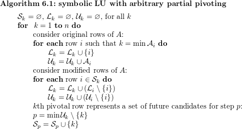
At the  $k$th step, partial pivoting can select any row whose leftmost non-zero falls in column
 $k$. Thus,
 ${\mathcal{U}}_{k}$ is the union of all such candidate pivot rows. This pivot row causes fill-in in all other candidate rows, which becomes the upper bound
 ${\mathcal{L}}_{k}$. Since these rows now all have the same non-zero pattern, their patterns are discarded and replaced with
 ${\mathcal{U}}_{k}$ itself. Thus, untouched rows of
 $A$ need only be considered once, and future steps need only look at the pattern of
 ${\mathcal{U}}_{k}$. The next time this row (representing a set of candidate pivot rows,
 ${\mathcal{L}}_{k}\setminus \{k\}$) is considered is at the step
 $p$ corresponding to the next non-zero entry in
 ${\mathcal{U}}_{k}$; namely,
 $p=\min {\mathcal{U}}_{k}\setminus \{k\}$. This is the first off-diagonal entry in the
 $k$th row of
 $U$. At that step
 $p$, the pattern
 ${\mathcal{U}}_{k}\setminus \{k\}$ is the upper bound of one (or more) unselected candidate pivot rows. The resulting algorithm takes time proportional to the upper bound on the LU factors,
 $O(|L|+|U|)$.
It should be noted that a single dense row destroys sparsity, causing this upper bound to become an entirely dense matrix. Such rows can be optimistically withheld, in an ad hoc manner, and placed as the last pivot rows. In this case, arbitrary partial pivoting is no longer possible.
Assuming the matrix  $A$ is strong-Hall, the column elimination tree for the LU factorization of
 $A$ is given by the expression
 $p=\min {\mathcal{U}}_{k}\setminus \{k\}$ in Algorithm 6.1 above, where
 $p$ is the parent of
 $k$, the first off-diagonal entry in the
 $k$th row of
 $U$. It is identical to the elimination tree of
 $A^{T}A$ in this case. If
 $A$ is not strong-Hall, the tree is not the same, and it is referred to as the row-merge tree instead. Grigori, Cosnard and Ng (Reference Grigori, Cosnard and Ng2007a) provide a general characterization of this row-merge tree and its properties, and describe an efficient algorithm for computing it. Grigori, Gilbert and Cosnard (Reference Grigori, Gilbert and Cosnard2009) consider cases where numerical cancellation can result in sparser LU factors, and they show that if numerical cancellation is ignored the row-merge tree provides a tight bound on the structure of
 $L$ and
 $U$.
Algorithm 6.1 provides an upper bound on the QR factorization of  $A$, as discussed in Section 7.1, which also gives an example of a matrix and its QR and LU factorizations as computed by this algorithm.
Gilbert and Liu (Reference Gilbert and Liu1993) generalize the elimination tree for a symmetric matrix to a pair of directed acyclic graphs (elimination DAGs, or EDAGs) for the LU factorization of an unsymmetric matrix (without pivoting). In LU factorization, the  $k$th row of
 $L$ can be constructed via a sparse triangular solve using the first
 $k-1$ columns of
 $U$, and the
 $k$th column of
 $U$ arises from a triangular solve with the first
 $k-1$ rows of
 $L$. This comes from an unsymmetric analogue of the up-looking Cholesky factorization, namely,
 $$\begin{eqnarray}\left[\begin{array}{@{}cc@{}}L_{11} & \\ l_{21} & 1\end{array}\right]\left[\begin{array}{@{}cc@{}}U_{11} & u_{12}\\ & u_{22}\end{array}\right]=\left[\begin{array}{@{}cc@{}}A_{11} & a_{12}\\ a_{21} & a_{22}\end{array}\right]\!,\end{eqnarray}$$
where all leading submatrices are  $(n-1)\times (n-1)$. Then the LU factorization can be computed with (1)
 $L_{11}U_{11}=A_{11}$ (a recursive LU factorization of the leading submatrix of
 $A$), (2)
 $L_{11}u_{12}=a_{12}$ (a sparse triangular solve for
 $u_{12}$), (3)
 $U_{11}^{T}l_{21}^{T}=a_{21}^{T}$ (a sparse triangular solve for
 $l_{21}$), and a dot product to compute
 $u_{22}$. As a result, the non-zero pattern of the
 $k$th row and
 $L$ and
 $k$th column of
 $U$ can be found as the reach in the acyclic graphs of
 $U$ and
 $L$, respectively, using equation (3.1). Basing a symbolic factorization on this strategy would result in a method taking the same time as the numeric factorization. Gilbert and Liu (Reference Gilbert and Liu1993) show how the graphs can be pruned via transitive reduction, giving the EDAGs (one for
 $L$ and another for
 $U$). For a symmetric matrix, the EDAGs are the same as the elimination tree of
 $A$. The transitive reduction of a graph preserves all paths (if
 $i{\rightsquigarrow}j$ is a path in a DAG, then a path still exists in the transitively reduced DAG). Gilbert and Liu (Reference Gilbert and Liu1993) characterize the row and column structures of
 $L$ and
 $U$ with these EDAGs, and present a left-looking symbolic factorization algorithm that constructs
 ${\mathcal{L}}$ and
 ${\mathcal{U}}$, building the EDAGs one node at a time. The EDAGs are more highly pruned graphs than the symmetric reductions of Eisenstat and Liu (Reference Eisenstat and Liu1992), but they take more time to compute.
Eisenstat and Liu (Reference Eisenstat and Liu2005a) provide a single tree that takes the place of the two EDAGs of Gilbert and Liu (Reference Gilbert and Liu1993). The symmetric elimination tree (a forest, actually) is given by edges in the Cholesky factor  $L$:
 $i$ is the parent of
 $k$ if
 $i$ is the first off-diagonal non-zero in column
 $k$ of
 $L$ (
 $\min \{i>k|l_{ik}\neq 0\}$). By contrast, Eisenstat and Liu’s single tree for LU (also technically a forest) is defined in terms of paths in
 $L$ and
 $U$ instead of edges in
 $L$. In this tree,
 $i$ is the parent of
 $k$ if
 $i>k$ is the smallest node for which there is a path in
 $L$ form
 $i$ to
 $k$, and also a path from
 $k$ back to
 $i$ in the graph of
 $U$. Analogous to the
 $k$th row subtree for a symmetric matrix, they characterize the non-zero patterns of the rows of
 $L$ and columns of
 $U$ in terms of sub-forests of this path-based elimination tree. In a sequel to this paper (Eisenstat and Liu Reference Eisenstat and Liu2008), they present an algorithm for constructing this path-based tree/forest, and show how it characterizes the graph of
 $L+U$ in a recursive bordered block triangular form.
Gilbert et al. (Reference Gilbert, Li, Ng and Peyton2001) describe an algorithm that computes the row and column counts for sparse QR and LU factorization, as an extension of their prior work (Gilbert et al. Reference Gilbert, Ng and Peyton1994). Details are given in Section 4.2.
Grigori et al. (Reference Grigori, Demmel and Li2007b) present a parallel symbolic LU factorization method, based on a left-looking approach of Gilbert and Liu (Reference Gilbert and Liu1993), which computes the  $k$th column of
 $L$ and the
 $k$th row of
 $U$ at the
 $k$th step. Their parallel algorithm generates a symbolic structure for
 $L$ and
 $U$ that can accommodate arbitrary partial pivoting. It starts with a vertex separator of the graph of
 $A+A^{T}$ to determine what parts of the symbolic factorization can be done in parallel. Vertex separators are an important tool for sparse direct methods and form the basis of the nested dissection ordering method discussed in Section 8.6.
6.2 Left-looking LU
The left-looking LU factorization algorithm computes  $L$ and
 $U$ one column at a time. At the
 $k$th step, it accesses columns 1 to
 $k-1$ of
 $L$ and column
 $k$ of
 $A$. If partial pivoting is ignored, it can be derived from the following 3
 $\times$ 3 block matrix expression, which is very similar to (5.1) for the left-looking Cholesky factorization algorithm. The matrix
 $L$ is assumed to have a unit diagonal:
 $$\begin{eqnarray}\left[\begin{array}{@{}ccc@{}}L_{11} & & \\ l_{21} & 1 & \\ L_{31} & l_{32} & L_{33}\end{array}\right]\left[\begin{array}{@{}ccc@{}}U_{11} & u_{12} & U_{13}\\ & u_{22} & u_{23}\\ & & U_{33}\end{array}\right]=\left[\begin{array}{@{}ccc@{}}A_{11} & a_{12} & A_{13}\\ a_{21} & a_{22} & a_{23}\\ A_{31} & a_{32} & A_{33}\end{array}\right]\!.\end{eqnarray}$$
The middle row and column of each matrix is the  $k$th row and column of
 $L$,
 $U$, and
 $A$, respectively. If the first
 $k-1$ columns of
 $L$ and
 $U$ are known, three equations can be used to derive the
 $k$th columns of
 $L$ and
 $U$:
 $L_{11}u_{12}=a_{12}$ is a triangular system that can be solved for
 $u_{12}$ (the
 $k$th column of
 $U$),
 $l_{21}u_{12}+u_{22}=a_{22}$ can be solved for the pivot entry
 $u_{22}$, and
 $L_{31}u_{12}+l_{32}u_{22}=a_{32}$ can then be solved for
 $l_{32}$ (the
 $k$th column of
 $L$). However, these three equations can be rearranged so that nearly all of them are given by the solution to a single triangular system:
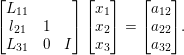 $$\begin{eqnarray}\left[\begin{array}{@{}ccc@{}}L_{11} & & \\ l_{21} & 1 & \\ L_{31} & 0 & I\end{array}\right]\left[\begin{array}{@{}c@{}}x_{1}\\ x_{2}\\ x_{3}\end{array}\right]=\left[\begin{array}{@{}c@{}}a_{12}\\ a_{22}\\ a_{32}\end{array}\right]\!.\end{eqnarray}$$
The solution to this system gives  $u_{12}=x_{1}$,
 $u_{22}=x_{2}$, and
 $l_{32}=x_{3}/u_{22}$. Partial pivoting with row interchanges is simple with this method. Once
 $x$ is found, entries in rows
 $k$ to
 $n$ can be searched for the entry with the largest magnitude. Permutation of the indices of
 $L$ is delayed until the end of the factorization. The non-zero patterns of the candidate pivot rows are not available (this would require a right-looking method) and thus the pivot row cannot be chosen for its sparsity. Fill-reducing orderings must instead be applied to the columns of
 $A$ only, as discussed in Section 8.5.
Relying on their optimal sparse triangular solve (Section 3.2), Gilbert and Peierls (Reference Gilbert and Peierls1988) show that their left-looking method takes time proportional to the number of floating-point operations. Other LU factorization methods can be faster in practice, but no other method provides this guarantee. This may seem like an obvious goal, but it can be quite difficult to achieve; it can take more time to search for entries and modify the data structure for  $L$ and
 $U$ than the floating-point work to compute them. This method was the first sparse LU factorization in MATLAB (Gilbert et al. Reference Gilbert, Moler and Schreiber1992). Recent versions of MATLAB no longer use it for
 , but it is still relied upon for the [L,U,P]=lu(A) syntax when A is sparse. When a column ordering is required, [L,U,P,Q]=lu(A) relies on UMFPACK instead (Davis and Duff Reference Davis and Duff1997, Reference Davis and Duff1999, Davis Reference Davis2004a, Reference Davis2004b, discussed in Section 11.4).
The earliest left-looking method by Sato and Tinney (Reference Sato and Tinney1963) did not accommodate any pivoting. Dembart and Neves (Reference Dembart, Neves and Anderson1977) show how the left-looking method can be implemented on a vector machine with hardware gather/scatter operations. Their method does take time proportional to the floating-point work, but only because they rely on a precomputed sparsity pattern of  $L$ and
 $U$. This restriction was lifted by Gilbert and Peierls’ (Reference Gilbert and Peierls1988) method. The first method to allow for partial pivoting was NSPIV by Sherman (Reference Sherman1978a, Reference Sherman1978b). It relied on a dynamic data structure with set unions performed as a merge operation, and as a result it could take more time than the floating-point work required. Sadayappan and Visvanathan (Reference Sadayappan and Visvanathan1988, Reference Sadayappan and Visvanathan1989) consider a parallel left-looking LU factorization method for circuit simulation matrices that does not allow for pivoting.
The majority of the methods described here (Sato and Tinney Reference Sato and Tinney1963, Sherman Reference Sherman1978a, Sherman Reference Sherman1978b, Sadayappan and Visvanathan Reference Sadayappan and Visvanathan1988, Eisenstat and Liu Reference Eisenstat and Liu1993a) actually store  $L$ and
 $U$ by rows and compute them one row at a time, but this is identical to the left-looking method applied to
 $A^{T}$.
Eisenstat and Liu (Reference Eisenstat and Liu1993a) reduce the work that Gilbert and Peierls’ (Reference Gilbert and Peierls1988) method requires for computing the reach in the graph of  $L$ when finding the pattern of
 $x$ (the
 $k$th column of
 $L$ and
 $U$) in the sparse triangular solve,
 ${\mathcal{X}}=\text{Reach}_{L}({\mathcal{B}})$. They observe that the reach of a node in the graph is unaffected if edges are pruned. For each
 $k$, let
 $i$ be the smallest index such that both
 $l_{ik}$ and
 $u_{ki}$ are non-zero. This entry forms a symmetric pair, or FSNZ(
 $k$) (Eisenstat and Liu Reference Eisenstat and Liu1992). Any entries below this in
 $L$ can be pruned from the graph of
 $L$, and the reach is unaffected. In the best case when the non-zero pattern of
 $L$ and
 $U$ is symmetric, this pruning results in the elimination tree, and the time to find the pattern
 ${\mathcal{X}}$ reduced to
 $O(|{\mathcal{X}}|)$.
Davis (Reference Davis2006) provides an implementation of the left-looking method of Gilbert and Peierls (Reference Gilbert and Peierls1988) in the CSparse package. It also forms the basis of KLU (Davis and Palamadai Natarajan Reference Davis and Palamadai Natarajan2010), a solver targeted for circuit simulation matrices. These matrices are too sparse for methods based on dense submatrices (supernodal, frontal, and multifrontal) to be efficient.
Gustavson, Liniger and Willoughby (Reference Gustavson, Liniger and Willoughby1970) and Hachtel, Brayton and Gustavson (Reference Hachtel, Brayton and Gustavson1971) present an alternative method for sparse LU factorization. Their symbolic analysis produces not only the non-zero patterns of the  $L$ and
 $U$, but also a loop-free code, with a sequence of operations that factorizes the matrix and is specific to its particular non-zero pattern. Norin and Pottle (Reference Norin and Pottle1971) consider fill-reducing orderings for this method. The method of generating loop-free code requires significant memory for the compiled code (proportional to the number of floating-point operations), which Gay (Reference Gay1991) shows is not required for obtaining good performance.
Chen, Wang and Yang (Reference Chen, Wang and Yang2013) present a multicore algorithm, NICSLU, based on the left-looking sparse LU. It accommodates partial pivoting during numerical factorization, and relies on the column elimination tree discussed in Section 6.1 for its parallel scheduling. Each task consists of one node in this tree, corresponding to the computation of a single column of  $L$ and
 $U$. The first phase handles nodes towards the bottom of this tree, one level at a time. In the second phase, each task updates its column with any prior columns that affect it and which have already completed. Prior columns not yet finished are skipped in the first pass of this task, and then handled in a second pass after they are complete.
6.3 Right-looking LU factorization with a static data structure
Gaussian elimination is a right-looking variant of LU factorization. At each step, an outer product of the pivot column and the pivot row is subtracted from the lower right submatrix of  $A$. After the
 $k$th step, the lower right submatrix
 $A^{[k]}$ is a Schur complement of the upper left
 $k\times k$ submatrix, also called the active submatrix. Numerical pivoting is typically essential, but ignoring it for the moment simplifies the derivation. The derivation of the method starts with an equation very similar to (4.2) for the right-looking Cholesky factorization,
 $$\begin{eqnarray}\left[\begin{array}{@{}cc@{}}l_{11} & \\ l_{21} & L_{22}\end{array}\right]\left[\begin{array}{@{}cc@{}}u_{11} & u_{12}\\ & U_{22}\end{array}\right]=\left[\begin{array}{@{}cc@{}}a_{11} & a_{12}\\ a_{21} & A_{22}\end{array}\right]\!,\end{eqnarray}$$
where  $l_{11}=1$ is a scalar, and all three matrices are square and partitioned identically. Other choices for
 $l_{11}$ are possible; this choice leads to a unit lower triangular
 $L$ and the four equations
 $$\begin{eqnarray}\displaystyle u_{11} & = & \displaystyle a_{11},\end{eqnarray}$$
 $$\begin{eqnarray}\displaystyle u_{12} & = & \displaystyle a_{12},\end{eqnarray}$$
 $$\begin{eqnarray}\displaystyle l_{21}u_{11} & = & \displaystyle a_{21},\end{eqnarray}$$
 $$\begin{eqnarray}\displaystyle l_{21}u_{12}+L_{22}U_{22} & = & \displaystyle A_{22}.\end{eqnarray}$$
Each equation is solved in turn, and can be expressed in MATLAB notation as the lu_right function below, where after the  $k$ step, A(k+1:n,k+1:n) holds the
 $k$th Schur complement,
 $A^{[k]}$.
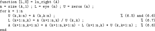
One advantage of the right-looking method over left-looking sparse LU factorization is that it can select a sparse pivot row and pivot column. The left-looking method does not keep track of the non-zero pattern of the  $A^{[k]}$ submatrix, and thus cannot determine the number of non-zeros in its pivot rows or columns. With pivoting of both rows and columns for the dual purposes of maintaining sparsity and ensuring numerical accuracy, the resulting factorization is
 $LU=PAQ$, where
 $Q$ is the column permutation. The disadvantage of the right-looking method is that it is significantly more difficult to implement, particularly when pivoting is done during numerical factorization. This variant is discussed in Section 6.4.
If the pivoting is determined prior to numeric factorization, however, then a simpler static data structure can be used for  $L$ and
 $U$. Eisenstat, Schultz and Sherman (Reference Eisenstat, Schultz, Sherman, Duff and Stewart1979) describe such a method that can be considered as a precursor to the multifrontal method (Section 11). It is a numeric form of their symbolic method (Eisenstat et al. Reference Eisenstat, Schultz, Sherman, Bunch and Rose1976a), which represents the symbolic graph elimination via a set of elements, or cliques that form during factorization. The method computes each update in a dense submatrix (much like the multifrontal method). To save space, it then discards the rows and columns of
 $L$ and
 $U$ inside these elements, except for the top-level separator. The rows and columns of
 $L$ and
 $U$ are then recalculated when needed.
With a static data structure, the right-looking method is more amenable to a parallel implementation, as compared to a dynamic data structure. Several of the earliest methods rely on pre-pivoting to enhance parallelism in a right-looking LU factorization by finding independent sets of pivots (Huang and Wing Reference Huang and Wing1979, Wing and Huang Reference Wing and Huang1980, Jess and Kees Reference Jess and Kees1982, Srinivas Reference Srinivas1983); none of these methods modify the pivot ordering during numeric factorization. In (6.4), the  $a_{11}$ scalar becomes an
 $s\times s$ diagonal matrix. This ordering strategy is discussed in Section 8.8, while we discuss the numeric factorization here.
Huang and Wing (Reference Huang and Wing1979) and Wing and Huang (Reference Wing and Huang1980) analyse the data dependencies in a fine-grained parallel method where each floating-point operation is a single task, either a division by the pivot,
 $$\begin{eqnarray}l_{ik}=\frac{a_{ik}^{[k]}}{u_{kk}},\end{eqnarray}$$
or an update to compute one entry in the Schur complement,
 $$\begin{eqnarray}a_{ij}^{[k]}=a_{ij}^{[k-1]}-l_{ik}u_{kj}.\end{eqnarray}$$
Each computation is placed in a directed acyclic graph, where the edges represent the data dependencies in these two kinds of computations, and a scheduling method is presented based on a local greedy heuristic. Note that several of these papers include the word ‘optimal’ in their title. This is an incorrect use of the term, since finding an optimal pivot ordering and an optimal schedule are NP-hard problems. Srinivas (Reference Srinivas1983) refines Wing and Huang’s (Reference Wing and Huang1980) scheduling method to reduce the number of parallel steps required to factorize the matrix.
Jess and Kees (Reference Jess and Kees1982) introduced the term elimination tree for their parallel right-looking LU factorization algorithm, which assumes a symmetric non-zero pattern. Their definition of the tree was limited to a filled-in graph of  $L+U$; this was later generalized by Schreiber (Reference Schreiber1982), who defined the elimination tree in the way it is currently used (Section 4.1). Jess and Kees used the tree for a coarse-grained parallel algorithm, where each node is a single step
 $k$ in the lu_right function above. Two nodes
 $k_{1}$ and
 $k_{2}$ can be executed in parallel if they do not share an ancestor/descendant relationship in the tree, and Jess and Kees define a method for scheduling the
 $n$ tasks. They note that two independent tasks can still require synchronization, however, since both can update the same set of entries in the lower right submatrix.
George and Ng (Reference George and Ng1985b) present a completely different approach for right-looking LU factorization by defining a static data structure for  $L$ and
 $U$ that allows for arbitrary row interchanges to accommodate numerical pivoting during factorization. This is based on a symbolic QR factorization, and they show that the non-zero pattern of
 $R$ for the QR factorization (
 $QR=A$) is an upper bound on the pattern of
 $U$ and
 $L^{T}$. In a companion paper, George et al. (Reference George, Liu and Ng1988b) refine this method with a more compact data structure. They demonstrate and exploit the fact that the pattern of
 $L$ is contained in the non-zero pattern of the
 $n$ Householder vectors (concatenated to form the matrix
 $V$) for the QR factorization. Their numeric factorization is much like the symbolic right-looking LU factorization method of Algorithm 6.1 in Section 6.1. At each step, they maintain a set of candidate pivot rows for each step
 $k$, analogous to the sets
 ${\mathcal{S}}_{1..n}$ in the symbolic LU factorization Algorithm 6.1. In that algorithm, the set of candidate pivot rows is replaced by a single representative row, since they all have the same non-zero pattern. In the numeric factorization, however, each row must be included. Instead of
 ${\mathcal{S}}_{k}$, the numeric factorization uses
 ${\mathcal{Z}}_{k}$ as the set of candidate pivot rows for step
 $k$. Initially,
 ${\mathcal{Z}}_{k}$ holds all original rows of
 $A$ whose leftmost non-zero entry resides in column
 $k$. At the
 $k$th step, one pivot row is chosen from
 ${\mathcal{Z}}_{k}$, and the remainder are added into the parent set
 ${\mathcal{Z}}_{p}$, where
 $p$ is the parent of
 $k$ in the column elimination tree.
George and Ng (Reference George and Ng1990) construct a parallel algorithm for their method, suitable for a shared-memory system. In contrast to the other papers on parallel algorithms discussed in this section, they describe an actual implementation. Their method relies on the fact that the sets  ${\mathcal{Z}}_{1:n}$ are always disjoint. Step
 $k$ of lu_right corresponds to node
 $k$ in the column elimination tree. If two nodes
 $a$ and
 $b$ do not have an ancestor/descendant relationship in the tree, and if all their descendants have been computed, then these two steps have no candidate pivot rows in common (
 ${\mathcal{Z}}_{a}$ and
 ${\mathcal{Z}}_{b}$ are disjoint). Each step selects one of their candidate pivot rows and uses it to update the remaining rows in their own set. This work for nodes
 $a$ and
 $b$ can be done in parallel.
6.4 Right-looking LU with dynamic pivoting
Unlike the left-looking method, the right-looking LU factorization method has the Schur complement available to it, in the active submatrix  $A^{[k]}$. It can thus select pivots from the entire active submatrix during factorization, using both sparsity and numerical criteria. For dense matrices, the complete pivoting strategy selects the entry in the active submatrix with the largest magnitude. The search for this pivot requires
 $O((n-k)^{2})$ work at the
 $k$th step, the same work as the subsequent numerical update.
6.4.1 Sequential right-looking methods with dynamic pivoting
For sparse matrices, the pivot search in a right-looking method with dynamic pivoting can far outweigh the numerical work, and thus care must be taken so that the search does not dominate the computation. Consider a sparse algorithm that examines all possible non-zeros in the active submatrix to search for the  $k$th pivot. This takes time proportional to the number of such non-zeros. In general this could be quite high, but it would at least have a loose upper of the number of entries in
 $L+U$. The numerical work for this pivot, however, would tend to be much lower. If the
 $k$th pivot row and column had just a handful of entries, the numerical update would take far less time since not all entries in the active submatrix need to be updated by this pivot, perhaps as few as
 $O(1)$. More precisely, let
 $A^{[k-1]}$ denote the active submatrix just prior to the
 $k$th step. If the
 $i$th row of
 $A^{[k-1]}$ contains
 $r_{i}$ non-zeros and the
 $j$th column contains
 $c_{j}$ non-zeros, then the numerical work for the
 $k$th step is precisely
 $2(r_{i}-1)(c_{j}-1)+(c_{j}-1)$. The terms
 $r_{i}$ and
 $c_{j}$ are called the row and column degrees, respectively.
Although searching the whole matrix for a pivot is far from optimal, this strategy forms the basis of the very first sparse direct method, by Markowitz (Reference Markowitz1957). Details of how the pivot is found are not given, but at the  $k$th step, the method selects
 $a_{ij}^{[k-1]}$ using two criteria: (1) the magnitude of this entry must not be too small, and (2) among those entries satisfying criterion (1), the pivot is selected that minimizes the Markowitz cost,
 $(r_{i}-1)(c_{j}-1)$.
Once this pivot is selected, the active submatrix is updated (line (6.8) in lu_right). Since the selection of this pivot is not known until the  $k$th step of numeric factorization, there is no bound for the non-zero pattern of
 $L$ and
 $U$, and a dynamic data structure must be used. These methods and data structures are very complex to implement, and various data structures and pivot selection strategies are reviewed by Duff (Reference Duff and Evans1985).
Tewarson (Reference Tewarson1966) takes a different approach that reduces the search. His method relies on the Gauss–Jordan factorization, which transforms  $A$ into the identity matrix
 $I$ rather than
 $U$ for LU factorization. However, the pivot selection problem is similar. His method selects a sparse column
 $j$, and then the entry of largest magnitude is selected as the pivot. The sparsity measure to select column
 $j$ is the sum row degrees for all non-zeros in this column. Since this is costly to update, it is computed just once, and then the column ordering is fixed from the beginning. Tewarson (Reference Tewarson1967a) considers alternatives: for example, after selecting column
 $j$, the non-zero pivot
 $a_{ij}$ with the smallest row degree
 $r_{i}$ is chosen, as long as its magnitude is large enough. Tewarson (Reference Tewarson1967c) changes focus to Gaussian elimination. He introduces the column intersection graph (the graph of
 $A^{T}A$) and proposes several pivot strategies based solely on this graph of the non-zero pattern of
 $A^{T}A$ (Section 8.5). He also proposes choosing as pivot the entry that causes the smallest amount of new non-zeros in
 $A^{[k]}$ (the minimal local fill-in criterion). Chen and Tewarson (Reference Chen and Tewarson1972b) generalize this strategy; their criterion is a combination of fill-in and the number of floating-point operations needed to eliminate the
 $k$th pivot.
The Gauss–Jordan factorization is no longer used in sparse matrix computations since Brayton, Gustavson and Willoughby (Reference Brayton, Gustavson and Willoughby1970) have proved that it always leads to a factorization with more non-zero entries than Gaussian elimination (that is, LU factorization).
Curtis and Reid (Reference Curtis and Reid1971) provide the details of their implementation of Markowitz’s pivot search strategy. Their data structure for the active submatrix allows for both rows and columns to be searched for the pivot with the least Markowitz cost, among those that are numerically acceptable. Duff and Reid (Reference Duff and Reid1974) compare this method with four others for selecting a pivot during a right-looking numeric factorization: minimum local fill-in, and three a priori column orderings. From their results, they recommend Markowitz’s strategy, which is indeed the dominant method for right-looking methods that select their pivots during numerical factorization.
Duff and Reid (Reference Duff and Reid1979b) use this strategy in MA28, which is probably the most well-used of all right-looking methods based on dynamic pivoting, along with its counterpart for complex matrices (Duff Reference Duff1981b). At first glance, it may seem that finding the pivot  $a_{ij}^{[k-1]}$ with minimal Markowitz cost
 $(r_{i}-1)(c_{j}-1)$ requires a search of all the non-zeros in
 $A^{[k-1]}$. This would be impractical. Duff and Reid (Reference Duff and Reid1979b) reduce this work via a branch-and-bound technique. Rows and columns are kept in a set of degree lists. Row
 $i$ is placed in the list with all other rows of degree
 $r_{i}$, and column
 $j$ is in the column list of degree
 $c_{j}$. The lists are updated as the factorization progresses, and thus finding the rows and columns of least degree is simple. However, finding a pivot requires the least product
 $(r_{i}-1)(c_{j}-1)$ among all those pivots whose numerical value passes a threshold test (the pivot
 $a_{ij}$ must have a magnitude of at least, say, 0.1 times the largest magnitude entry in column
 $j$). Their method first looks in the sparsest column and finds the candidate pivot with best Markowitz cost. It then searches the sparsest row, then the next sparsest column, and so on. Let
 $r$ and
 $c$ be the row and column degrees of the sparsest rows and columns still being searched, respectively, and let
 $M$ be the best Markowitz cost found so far. If
 $M\leq (r-1)(c-1)$ then the search can terminate, since no other pivots can have a lower Markowitz cost than
 $M$. It is still possible that the entire matrix could be searched, but in practice the search terminates quickly.
Zlatev (Reference Zlatev1980) modifies this method by limiting the search to just a few of the sparsest columns (4, say), implementing this in the Y12M software package (Osterby and Zlatev Reference Osterby and Zlatev1983). Zlatev and Thomsen (Reference Zlatev, Thomsen and Duff1981) considers a drop tolerance, where entries with small magnitude are deleted during numerical factorization (thus saving time and space), followed by iterative refinement (Zlatev Reference Zlatev and Evans1985).
Kundert (Reference Kundert and Ruehli1986) relies on the Markowitz criterion in his right-looking factorization method, but where the diagonal entries are searched first. This strategy is well-suited to the matrices arising in the SPICE circuit simulation package for which the method was developed.
The most recent implementation of the dynamic-pivoting, right-looking method is MA48 by Duff and Reid (Reference Duff and Reid1996a). It adds several additional features, including a switch to a dense matrix method when the active submatrix is sufficiently dense. Pivoting can be restricted to the diagonal, reducing the time to perform the search and decreasing fill-in for matrices with mostly symmetric non-zero pattern.
Many LU factorization methods (those discussed here, and supernodal and multifrontal methods discussed later) rely on a relaxed partial pivoting criterion where the selected pivot need not have the largest magnitude in its column. Even left-looking methods use it because it allows preference for selecting the diagonal entry as pivot, which in practice reduces fill-in for matrices with symmetric non-zero pattern (Duff Reference Duff, Glowinski and Lions1984c). A relaxed partial pivoting strategy allows for freedom to select a sparse pivot row, thus reducing time and memory requirements, but it can sometimes lead to numerical inaccuracies. Arioli, Demmel and Duff (Reference Arioli, Demmel and Duff1989a) resolve this problem with an inexpensive algorithm that computes an accurate estimate of the sparse backward error. The estimate provides a stopping criterion for iterative refinement. For most matrices the error estimate is low, and no iterative refinement is needed at all. In MATLAB,  uses this strategy when A is unsymmetric, as implemented in UMFPACK (Davis and Duff Reference Davis and Duff1997, Davis Reference Davis2004a).
6.4.2 Parallel right-looking methods with dynamic pivoting
With a dynamic data structure and little or no symbolic pre-analysis, the right-looking LU factorization method is even more complex to implement in a parallel algorithm. However, several methods have been developed that tackle this challenge.
Davis and Davidson (Reference Davis and Davidson1988) exploit parallelism in both the pivot search and numerical update. Each task selects two of the sparsest rows whose leftmost non-zero falls in the same column, and uses one row to eliminate the leftmost non-zero in the other row (pairwise pivoting). Fill-in is controlled since the two rows are selected in order of their row degree. Parallelism arises because there are many such pairs.
Kruskal, Rudolph and Snir (Reference Kruskal, Rudolph and Snir1989) consider a theoretical EREW model of parallel computing in a method that operates on a single pivot at a time (each floating-point update is considered its own task). They do not discuss an implementation.
Several methods find independent set of pivots during numeric factorization (Alaghband Reference Alaghband1989, Alaghband and Jordan Reference Alaghband and Jordan1989, Davis and Yew Reference Davis and Yew1990, Van der Stappen, Bisseling and van de Vorst Reference Van der Stappen, Bisseling and van de Vorst1993, Koster and Bisseling Reference Koster and Bisseling1994). In a single step, a set of pivots is found such that they form a diagonal matrix in the upper left corner when permuted to the diagonal. The updates from these pivots can then be computed in parallel, assuming that parallel updates to the same entry in the active submatrix are either synchronized, or performed by the same processor. These methods are related to methods that find such sets prior to factorization, an ordering method discussed in Section 8.8.
Alaghband (Reference Alaghband1989) and Alaghband and Jordan (Reference Alaghband and Jordan1989) use a binary matrix to find compatible pivots, which are constrained to the diagonal. Alaghband (Reference Alaghband1995) extends this method to allow for sequential unsymmetric pivoting to enhance numerical stability. Davis and Yew (Reference Davis and Yew1990) rely on a parallel Markowitz search, where each processor searches independently, and pivots may reside anywhere in the matrix. Two processors may choose two pivots that are not compatible with each other (causing the submatrix of pivots to no longer be diagonal). To avoid this, when a candidate pivot is found, it is added to the pivot set in a critical section that checks this condition. The downside of Davis and Yew’s (Reference Davis and Yew1990) approach is that the pivots are selected non-deterministically, which results in a different pivot sequence if the same matrix is factorized again. Both the methods of Alaghband et al. and Davis et al. rely on a shared-memory model of computing. Van der Stappen et al. (Reference Van der Stappen, Bisseling and van de Vorst1993) and Koster and Bisseling (Reference Koster and Bisseling1994) develop a distributed-memory algorithm for finding and applying these independent sets to factorize a sparse matrix on a mesh of processors with communication links, and no shared memory.
An entirely different approach for a parallel right-looking method is to partition the matrix into independent blocks and to factorize the blocks in parallel. Duff’s (Reference Duff, Evans and Sutti1989c) method permutes the matrix into bordered block triangular form, and then factorizes each independent block with MA28. Geschiere and Wijshoff (Reference Geschiere and Wijshoff1995), Gallivan, Hansen, Ostromsky and Zlatev (Reference Gallivan, Hansen, Ostromsky and Zlatev1995), and Gallivan, Marsolf and Wijshoff (Reference Gallivan, Marsolf and Wijshoff1996) also do this in MCSPARSE. The diagonal blocks are factorized in parallel, followed by the factorization of the border, which is a set of rows that connect the blocks. Duff and Scott (Reference Duff and Scott2004) use a similar strategy in MP48, a parallel version of MA48. They partition the matrix into single-bordered block diagonal form and then use MA48 in parallel on each block.
7 QR factorization and least-squares problems
In QR factorization, the matrix  $A$ is factorized into the product
 $A=QR$, where
 $Q$ is orthogonal and
 $R$ is upper triangular. Sparse QR factorization is the method of choice for sparse least-squares problems, underdetermined systems, and for solving sparse linear systems when
 $A$ is very ill-conditioned.
The orthogonal matrix  $Q$ has the property that
 $Q^{T}Q=I$, and thus
 $Q^{-1}=Q^{T}$. This makes it simple to solve
 $Qx=b$ by just computing
 $x=Q^{T}b$. For sparse matrices,
 $Q$ is typically formed implicitly as a product of a set of Householder reflections or Givens rotations, although a few papers discussed below consider the Gram–Schmidt process. In a sparse least-squares problem, the goal is to find
 $x$ that minimizes
 $\Vert b-Ax\Vert$, and if
 $b$ is available when
 $A$ is factorized, space can be saved by discarding
 $Q$ as it is computed, by simply applying the transformations to
 $b$ as they are computed. After QR factorization, the least-squares problem is solved by solving
 $Qy=b$, and then the sparse triangular system
 $Rx=y$. Alternatively, the corrected semi-normal equations can solve a least-squares problem if
 $Q$ is discarded, even if
 $b$ is not available when
 $A$ is factorized.
Prior to considering the details of the many methods for symbolic analysis and numeric factorization for sparse QR factorization, it is helpful to take a quick look at two numeric methods first: a sparse row-oriented method based on Givens rotations, and a column-oriented method for dense matrices based on Householder reflections. These two methods motivate the symbolic analysis for sparse QR factorization discussed in Section 7.1. Further details of the row-oriented numeric QR factorization based on Givens rotations are presented in Section 7.2, and a column-oriented sparse QR factorization using Householder reflections is presented in Section 7.3. The latter is not often used in practice in its basic form, but the method is related to the sparse multifrontal QR factorization (Section 11.5). QR is well-suited for handling rank-deficient problems, although care must be taken because column pivoting destroys sparsity, which we discuss in Section 7.4. Sparse QR factorization can be costly, and thus several alternatives to QR factorization have been presented in the literature: the normal equations, solving an augmented system via symmetric indefinite ( $\text{LDL}^{\text{T}}$) factorization, and relying on LU factorization. These alternative methods are discussed in Section 7.5.
Sparse row-oriented QR factorization with Givens rotations
George and Heath (Reference George and Heath1980) present the first row-oriented QR factorization, based on Givens rotations, and it can be simply described (hereafter referred to as the row-Givens method). Row-Givens starts with a symbolic analysis of the normal equations, since under a few simplifying assumptions, the non-zero pattern of  $R$ is given by the Cholesky factor of
 $A^{T}A$. All of the methods for Cholesky symbolic analysis in Section 4 can thus be used on
 $A^{T}A$, and the pattern
 ${\mathcal{R}}$ of
 $R$ is known prior to numeric factorization.
The numeric factorization starts with an  $R$ that is all zero, but with a known final non-zero pattern. It is stored row-by-row in a static data structure. The method selects a row of
 $A$ and finds its leftmost non-zero; suppose this entry is in column
 $k$. This entry is annihilated with a Givens rotation (a 2
 $\times$ 2 orthogonal matrix
 $G$) that uses the
 $k$th row of
 $R$ to annihilate the
 $k$ entry of the selected row of
 $A$. Both rows are modified. The next leftmost entry in this row of
 $A$ is then found, and the process continues until the row of
 $A$ has been annihilated to zero. If the diagonal
 $r_{kk}$ is zero, the Givens rotation becomes a swap. This happens if the
 $k$th row of
 $R$ is all zero, and thus the process stops early.
The MATLAB rowgivens script below illustrates the row-Givens sparse QR factorization. To keep it simple, it does not consider the pattern of  $R$ and stores R in dense format. However, it does consider the sparsity of the rows of A. The function implicitly stops early if it encounters a zero on the diagonal of R. The matrix
 $Q$ could be computed, or kept implicitly as a sequence of Givens rotations, but the script simply discards it.
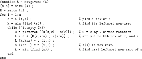
Dense column-oriented QR factorization with Householder reflections
A Householder reflection is a symmetric orthogonal matrix of the form  $H=I-{\it\beta}vv^{T}$, where
 ${\it\beta}$ is a scalar and
 $v$ is a column vector. The vector
 $v$ and scalar
 ${\it\beta}$ can be chosen based on a vector
 $x$ so that
 $Hx$ is zero except for the first entry
 $(Hx)_{1}=\pm \Vert x\Vert _{2}$. Computing the matrix–vector product
 $Hx$ takes only
 $O(n)$ work. The non-zero patterns of
 $v$ and
 $x$ are the same. The MATLAB script qr_right_householder uses Householder reflections in a right-looking manner to compute the QR factorization. It represents
 $Q$ implicitly as a sequence of Householder reflections (V and Beta) which could be discarded if they are not needed. Householder reflections can also be used for a left-looking QR factorization, assuming they are all kept.

7.1 Symbolic analysis for QR
The row/column count algorithm for sparse Cholesky factorization was considered in Section 4.2. The method can also be extended for the QR and LU factorization of a square or rectangular matrix  $A$. For QR factorization, the non-zero pattern of
 $R$ is identical to
 $L^{T}$ in the Cholesky factorization
 $LL^{T}=A^{T}A$, assuming no numerical cancellation and assuming the matrix
 $A$ is strong-Hall (that is, it cannot be permuted into block upper triangular form with more than one block). This same matrix
 $R$ provides an upper bound on the non-zero pattern of
 $U$ for an LU factorization of
 $A$. The inter-relationships of symbolic QR, LU, and Cholesky factorization, and many other results in this section, are surveyed by Gilbert and Ng (Reference Gilbert, Ng, George, Gilbert and Liu1993), Gilbert (Reference Gilbert1994), and Pothen and Toledo (Reference Pothen, Toledo, Mehta and Sahni2004).
Forming  $A^{T}A$ explicitly can be very expensive, in both time and memory. Fortunately, Gilbert et al. (Reference Gilbert, Li, Ng and Peyton2001) show that this is not required for finding the column elimination tree or the row/column counts of
 $R$ (and thus bounds on
 $U$ for LU). Each row
 $i$ of
 $A$ defines a clique in the graph of
 $A^{T}A$, but not all of these entries will appear in the skeleton matrix of
 $A^{T}A$. The column elimination tree is the tree for
 $R$, and is the same as the Cholesky factor of
 $A^{T}A$. To compute the column elimination tree, each clique is implicitly replaced with a path amongst its nodes. Each row of
 $A$ thus lists the nodes (columns) in a single path, and using this new graph gives the elimination tree of the Cholesky factor of
 $A^{T}A$.
For the row/column counts, Gilbert et al. (Reference Gilbert, Li, Ng and Peyton2001) form a star matrix with  $O(|A|)$ entries, but whose factorization has the same pattern as that of
 $A^{T}A$. The
 $k$th row and column of the star matrix is the union of rows in
 $A$ whose leftmost non-zero entry appears in column
 $k$. Thus, the row/column counts for QR and the bounds on LU can be found in nearly
 $O(|A|)$ time as well. With this method the original matrix
 $A$ can be used, taking only
 $O(|A|)$ space, which is much less than
 $O(|A^{T}A|)$.
Tewarson (Reference Tewarson1968) and Chen and Tewarson (Reference Chen and Tewarson1972a) present the first analysis of the sparsity of two column-wise right-looking QR factorization methods, one based on Householder reflections and the other on the Gram–Schmidt method. The two methods produce a similar matrix  $Q$. However, Gram–Schmidt constructs
 $Q$ explicitly, whereas the Householder reflections implicitly represent
 $Q$ in a much sparser form. They also consider column pre-orderings to reduce fill-in in
 $Q$ and
 $R$ (Section 8.5).
Coleman, Edenbrandt and Gilbert (Reference Coleman, Edenbrandt and Gilbert1986) characterize the pattern of  $R$ of the row-Givens QR. They show that the Cholesky factor of
 $A^{T}A$ is a loose upper bound on the fill-in of
 $R$ when
 $A$ is not strong-Hall (that is, when it can be permuted into block triangular form with more than one diagonal block). The rowgivens algorithm can be symbolically simulated using a local Givens rule: both rows that participate in a Givens reduction take on the non-zero pattern of the union of both of them (except for the one annihilated entry). They prove that the local Givens rule correctly computes the fill-in if
 $A$ is strong-Hall, but it may also overestimate the final pattern of
 $R$ otherwise. They then show that the local Givens rule gives an exact prediction if
 $A$ is first permuted into block triangular form (Section 8.7.3).
In row-Givens the matrix  $R$ starts out all zero, and only at the end of factorization does it take on its final non-zero pattern. The column ordering alone determines this final pattern. However, the order in which the rows are processed affects the intermediate fill-in, as the pattern of each row of
 $R$ grows from the empty set to its final form. Ostrouchov (Reference Ostrouchov1993) considers row and column pre-orderings for row-Givens, which are discussed in Section 8.5. He also characterizes the exact structure of the intermediate fill-in of each row of
 $A$ in a right-looking QR factorization. His focus is on Givens rotations but his analysis also holds for the right-looking column-Householder method. At step
 $k$, the non-zero pattern of A(k:m,k) determines the pattern of the
 $k$th Householder vector. It also gives the set of rows that must take part in a right-looking row-Givens reduction. His concise data structure is based on the following observation. After all these entries are annihilated (except for the diagonal), all these rows take on the non-zero pattern of the set union of all of them, minus the annihilated
 $k$ column itself (which remains only in the
 $k$th row of
 $R$, as the diagonal).
George and Ng (Reference George and Ng1987) rely on this same observation for a symbolic right-looking LU factorization, in which the non-zero patterns of all pivot row candidates at the  $k$th step are replaced with the set union of all such rows. They note that this process gives upper bounds
 $\hat{L}$ and
 $\hat{U}$ on the structure of
 $L$ and
 $U$ with partial pivoting, and also exactly represents the intermediate fill-in for a right-looking QR factorization. It gives a tighter estimate of the pattern of
 $R$ than the Cholesky factors of
 $A^{T}A$. They describe an
 $O(|\hat{L}|+|\hat{U} |)$-time symbolic algorithm for constructing the pattern of the upper bounds, which also gives the pattern of
 $R$ for QR factorization in
 $O(|R|)$ time (Algorithm 6.1: symbolic LU factorization with arbitrary partial pivoting, in Section 6.1). The algorithm also constructs the non-zero pattern of the Householder vectors,
 $V$, which is an upper bound for
 $L$. More precisely, the upper bound
 ${\mathcal{L}}_{k}$ is exactly the same as the non-zero pattern of the
 $k$th Householder vector.
Figure 7.1 shows a QR factorization using Householder vectors: (a) the original matrix  $A$, (b) its column elimination tree, and (c) the factor
 $R$ (in the upper triangular part) and the set of Householder vectors
 $V$ (in the lower triangular part) used to annihilate
 $A$ to obtain
 $R$. These same structures give upper bounds on the pattern of
 $L$ and
 $U$ for LU factorization with arbitrary partial pivoting via row interchanges during numeric factorization. The non-zero pattern of
 $V$ is an upper bound for
 $L$, and the pattern of
 $R$ is an upper bound for
 $U$. These upper bounds are computed by Algorithm 6.1.
(a) A sparse matrix  $A$, (b) its column elimination tree, and (c) its QR factorization (
 $R$ denotes the upper triangular part and
 $V$ the Householder vectors in the lower triangular part) (Davis Reference Davis2006).
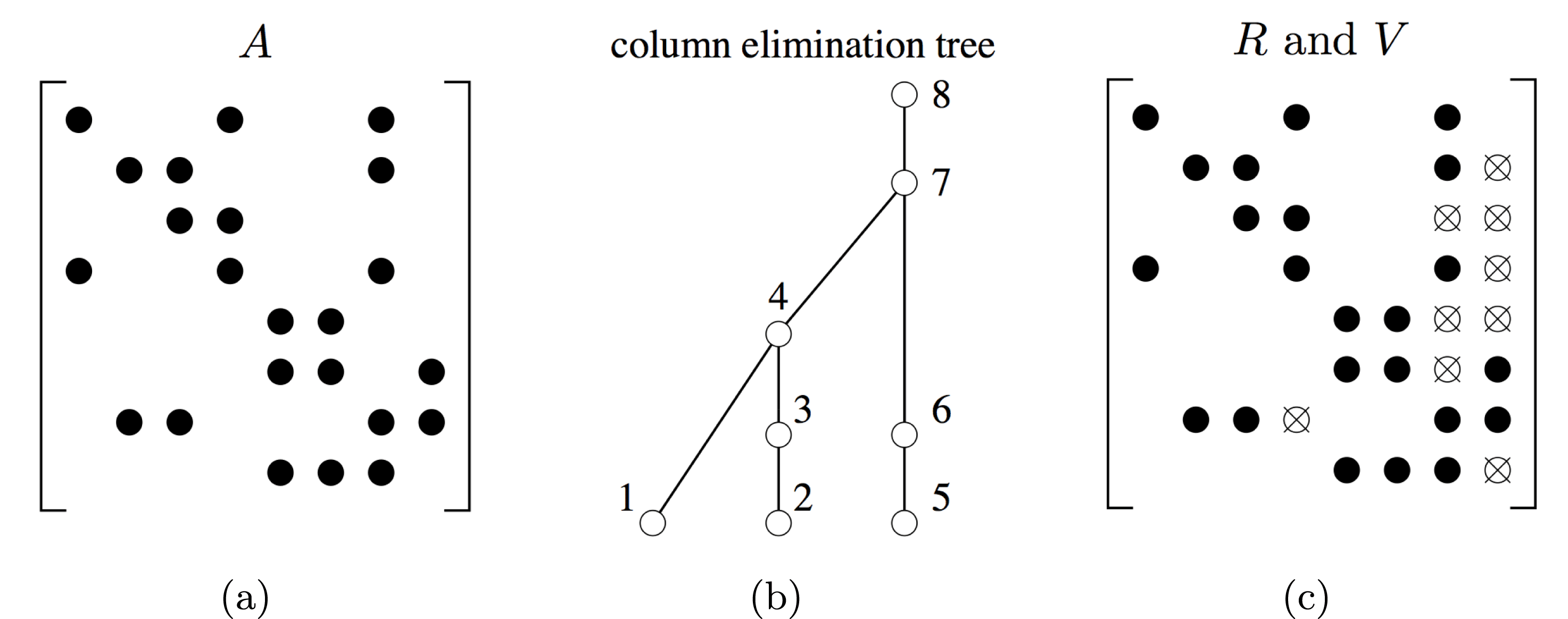
For the right-looking Householder method (qr_right_householder), the columns of  $V$ represent the set of Householder reflections, which provides an implicit representation of
 $Q$. George et al. (Reference George, Liu and Ng1988b) show that the sparsity pattern of each row of
 $V$ is given by a path in the column elimination tree. For row
 $i$, the path starts at the node corresponding to the column index of leftmost non-zero entry,
 $j=\min {\mathcal{A}}_{i}$. It proceeds up the tree, terminating at node
 $i$ if
 $i\leq n$, and at a root of the tree otherwise. The non-zero patterns of the columns are defined by George and Ng (Reference George and Ng1987): the pattern
 ${\mathcal{V}}_{k}$ is the union of the pattern
 ${\mathcal{V}}_{c}$ of each child
 $c$ of node
 $k$ in the column elimination tree, and also the entries in the lower triangular part of
 $A$.
Hare, Johnson, Olesky and van den Driessche (Reference Hare, Johnson, Olesky and van den Driessche1993) provide a tight characterization of the sparsity pattern of QR factorization when  $A$ has full structural rank (or weak-Hall) but might not be strong-Hall. Matrices with this property can be permuted so that they have a zero-free diagonal, and they have a non-zero pattern such that there exists an assignment of numerical values so that they have full numeric rank. Their results have a one-at-a-time property, in that for each predicted non-zero in
 $Q$ and
 $R$, there exists a matrix with the same pattern of
 $A$ that makes this entry actually non-zero. Pothen (Reference Pothen1993) shows that the results of Hare et al. (Reference Hare, Johnson, Olesky and van den Driessche1993) hold in an all-at-once sense, in that there is a single matrix
 $A$ that makes all the predicted non-zeros in
 $Q$ and
 $R$ non-zero. Thus, these results are as tight as possible without considering the values of
 $A$.
Ng and Peyton (Reference Ng and Peyton1992, Reference Ng and Peyton1996) extend the results of Hare et al. (Reference Hare, Johnson, Olesky and van den Driessche1993) to provide an explicit representation of the rows of  $Q$, based on the row structure of
 $V$. They first generalize the column elimination tree (with
 $n$ nodes, one per column, if
 $A$ is
 $m\times n$) to a new tree with
 $m$ nodes. The tree is the same for nodes with parents in the column elimination tree. The remaining nodes have as their parent the next non-zero row in the first Householder vector
 $V$ that modifies them. They show that row
 $i$ of
 $Q$ is given by the path from node
 $k$ to the root of this generalized tree, where
 $k$ is the first Householder vector that modifies row
 $i$. They also show that George and Ng’s (Reference George and Ng1987) symbolic LU and QR factorization algorithm (Algorithm 6.1 in Section 6.1) provides tight bounds on the pattern of
 $V$ and
 $R$ if the matrix
 $A$ is first permuted into block upper triangular form.
Oliveira (Reference Oliveira2001) provides an alternative method that does not require that the matrix be permuted into this block triangular form, but modifies the row-merge tree of Algorithm 6.1 instead to obtain the same tight bounds. Her method prunes edges in the row-merge tree. Each node of the row-merge tree represents the elimination of a set of rows of  $A$. If the leftmost non-zero in row
 $i$ is
 $k$, then it starts at node
 $k$ of the tree. One row is selected as a pivot, and the remainder are sent to the parent. If the count of rows at a node goes to zero, then it is given no parent in this modified row-merge tree. Row
 $k$ ‘evaporates’ when the set
 ${\mathcal{S}}_{k}$ turns out to be empty.
Gilbert, Ng and Peyton (Reference Gilbert, Ng and Peyton1997) compare and contrast the implicit representation of  $Q$ (as the set of Householder vectors
 $V$), and the explicit representation of
 $Q$ (as a matrix). The implicit representation is normally sparser. They give a theoretical distinction as to when this is the case, based on the size of vertex separators of the graph of
 $A^{T}A$. Vertex separators for QR factorization are an integral part of the nested dissection method discussed in Section 8.6.2.
7.2 Row-oriented Givens-based QR factorization
George and Heath (Reference George and Heath1980) developed the first QR factorization based on Givens rotations, as already discussed in the introduction to Section 7, and as illustrated in the rowgivens function. The method has been extended and studied in many related papers since then, which we discuss here. Fill-reducing pre-orderings for this method based solely on the non-zero pattern of  $A$ are considered in Section 8, but some methods find their pivot orderings during numeric factorization, for reducing fill-in, improving accuracy, or for handling rank-deficient problems. These pivot strategies are considered here.
Duff (Reference Duff1974b) considers several methods for ordering the rows and columns when computing the QR factorization via Givens rotations. Different row orderings give the same upper triangular factor  $R$, but result in different amounts of intermediate fill-in as the factorization progresses, and different amounts of total floating-point work that needs to be performed. Each major step annihilates a single column. In each method, a single pivot row is chosen at the
 $k$th major step, and used to annihilate all non-zeros in column
 $k$ below it. Duff considers the natural order (as given in the input matrix), ascending number of non-zeros in each target row, and a minimum fill-in ordering in which the next row selected as the target is the one that will cause the least amount of new fill-in in the pivot row. Five column pre-orderings are also presented. The simplest is to pre-order the columns by ascending column count, which does not give good results. Four methods are employed during the QR factorization, and operate on the updated matrix as it is reduced to upper triangular form. Let
 $r_{i}$ denote the number of entries in row
 $i$, and
 $c_{j}$ the number of entries in column
 $j$. The four methods are: (1) the sparsest column is selected, and then within that column, the sparsest row is selected, (2) the reverse of method (1), (3) the entry with the smallest Markowitz cost is selected (
 $r_{i}c_{j}$), and (4) the entry with the smallest metric
 $r_{i}c_{j}^{2}$. Method (1) is shown to be the best overall.
Gentleman (Reference Gentleman and Watson1975) presents a variable pivot row strategy. For each Givens rotation within the  $k$th major step, the two rows chosen are the two sparsest rows whose leftmost non-zero lies in column
 $k$.
Zlatev (Reference Zlatev1982) considers two pivotal strategies. Both are done during factorization, with no symbolic pre-analysis or ordering phase (this is in contrast to George and Heath’s (Reference George and Heath1980) method, which assumes both steps are performed). The goal of Zlatev’s (Reference Zlatev1982) strategies is to reduce intermediate fill-in. One strategy selects the column of least degree (fewest non-zeros), and then picks two rows of least degree with leftmost non-zero entry in this column and applies a Givens rotation to annihilate the leftmost non-zero entry in one of the two rows. The next pair of rows can come from a different column. In his second strategy, a column of least degree is selected and the sparsest row is selected as the pivot row from the set of rows whose leftmost non-zero is in this column. This pivot row is used to annihilate the leftmost non-zero in all the other rows, in increasing order of their degree.
Robey and Sulsky (Reference Robey and Sulsky1994) develops a variable pivot row strategy that extends Gentleman’s (Reference Gentleman and Watson1975) idea. At each major step, the two pivot rows are chosen that cause the least amount of fill in both of the two rows. Thus, two rows with many non-zeros but with the same pattern would be selected instead of two very sparse rows that have different patterns.
Some row orderings can result in intermediate fill-in that is not restricted to the final pattern of  $R$. This can lead to an increase in storage. Gillespie and Olesky (Reference Gillespie and Olesky1995) describe a set of conditions on the row ordering that ensure the intermediate fill-in is restricted to the non-zero pattern of
 $R$.
George, Heath and Plemmons (Reference George, Heath and Plemmons1981) consider an out-of-core strategy. In George and Heath’s (Reference George and Heath1980) method, a single row of  $A$ is processed at a time and it is annihilated until it is all zero or until it lands in an empty row for
 $R$. Since the rows of
 $A$ in George and Heath’s (Reference George and Heath1980) method are fully processed, one at a time, it is well-suited to George et al.’s (Reference George, Heath and Plemmons1981) out-of-core strategy where
 $A$ is held in auxiliary memory. They employ a nested dissection ordering (George et al. Reference George, Poole and Voigt1978), discussed in Section 8.6, to partition the problem so that only part of
 $R$ need reside in main memory at any one time. A row of
 $A$ may be processed more than once, since only part of
 $R$ is held. In this case, it is written to a file, and read back in again for the next phase.
Heath (Reference Heath1982) extends the method of George and Heath (Reference George and Heath1980) to handle rank-deficiency. Modifying the column permutation would be the best strategy, numerically speaking, by selecting the next pivot column as the column of largest norm. Column pivoting is relied upon for rank-deficient dense matrices, and it is very accurate. However, the column ordering for the sparse case is fixed, prior to factorization. Changing it breaks the symbolic analysis entirely. The solution is to keep the same column ordering, but to produce an  $R$ with different (and fewer) rows. Consider the Givens rotation G in rowgivens, which uses the
 $k$th row of
 $R$ to annihilate s(k). Suppose that R(k,k) is zero and s(k) is already zero or nearly so. The Givens rotation is skipped, and the
 $k$th row of
 $R$ remains empty. The entry s(k) is set to zero and the row s proceeds to the next row. If
 $A$ is found to be rank-deficient, the resulting
 $R$ will have gaps in it, with empty rows. These rows are deleted to obtained the ‘squeezed’
 $R$. When factorization is complete, the corresponding columns can be permuted to the end, and
 $R$ becomes upper trapezoidal. MATLAB uses this strategy for
 , when it encounters a sparse rectangular rank-deficient matrix (Gilbert et al. Reference Gilbert, Moler and Schreiber1992, Davis Reference Davis2011a).
Dense rows of  $A$ can cause
 $R$ to become completely non-zero, destroying sparsity. Björck (Reference Björck1984) avoids this problem by withholding them from the sparse QR factorization when solving a least-squares problem, and then adding them back in via non-orthogonal eliminations.
Sparse QR is not limited to solving least-squares problems. Suppose  $A$ is
 $m\times n$ with
 $m<n$. If
 $A$ has full rank, the system
 $Ax=b$ is underdetermined and there are many solutions, but a unique solution of minimum norm exists. George, Heath and Ng (Reference George, Heath and Ng1984a) employ a sparse QR factorization of
 $A^{T}$, giving an LQ factorization
 $A=LQ$ that is suitable for finding this minimum norm solution. If
 $A$ is rank-deficient, then rank-deficiency handling (Heath Reference Heath1982) and column updating (Björck Reference Björck1984) (see Section 7.4), along with a subsequent sparse LQ factorization of a smaller matrix if necessary, can find a solution. In each case, arbitrary column pivoting is avoided during numerical factorization, thus keeping the symbolic pre-analysis valid.
Liu (Reference Liu1986c) generalizes row-Givens by treating blocks of rows. Each block becomes a full upper trapezoidal submatrix, and pairs of these are merged via a Givens-based method that produces a single upper trapezoidal submatrix. Since this is a right-looking method that employs dense submatrices, it is very similar to the Householder-based multifrontal QR factorization (Section 11.5), in which each submatrix becomes a frontal matrix, and where more than two are merged at a time.
Ostrouchov (Reference Ostrouchov1993) presents a bipartite graph model for analysing row orderings performed in the numerical factorization phase of row-Givens, in contrast to row pre-orderings that are computed prior to factorization (the latter are discussed in Section 8.5).
Several parallel versions of row-Givens have been implemented. The first was a shared-memory algorithm by Heath and Sorensen (Reference Heath and Sorensen1986), where multiple rows of  $A$ are eliminated in a pipelined fashion. Each processor has its own row of
 $A$, and synchronization ensures that each processor has exclusive access to one row of
 $R$ at a time. For a distributed-memory model, Chu and George (Reference Chu and George1990) extend the general row-merge method of Liu (Reference Liu1986c). Subtrees are given to each processor to handle independently, and further up the tree, the pairwise merge of two upper trapezoidal submatrices is spread across all processors. Kratzer (Reference Kratzer1992) uses the row-wise method of George and Heath (Reference George and Heath1980) for a SIMD parallel algorithm. Each row can participate in multiple Givens rotations at one time, via pipelining. This is contrast to the pipelined method of Heath and Sorensen (Reference Heath and Sorensen1986), which treats an entire row as a single unit of computation. Kratzer and Cleary (Reference Kratzer, Cleary, George, Gilbert and Liu1993) include this method in their survey of SIMD methods for sparse LU and QR factorization. Ostromsky, Hansen and Zlatev (Reference Ostromsky, Hansen and Zlatev1998) permute the matrix into a staggered block staircase form, by sorting the rows according to their leftmost non-zero entry. This results in a matrix where the leading blocks may be rectangular and where the lower left corner is all zero. Each of the block rows are factorized in parallel. This moves the staircase towards becoming upper triangular, but does not necessarily result in an upper triangular matrix, so the process is repeated until the matrix becomes upper triangular.
7.3 Column-oriented Householder-based QR factorization
The column-oriented Householder factorization can be implemented via either a right-looking (as qr_right_householder) or left-looking strategy. In its pure non-multifrontal form discussed here it is not as widely used as row-Givens. However, the right-looking variant forms the basis of the sparse multifrontal QR, a widely used right-looking algorithm discussed in Section 11.5. The method has one distinct advantage over row-Givens: it is much easier to keep the Householder reflections, which represent  $Q$ in product form as a collection of Householder vectors (
 $V$) and coefficients, than it is to keep all the Givens rotations.
The method was first considered by Tewarson (Reference Tewarson1968) and Chen and Tewarson (Reference Chen and Tewarson1972a), who analysed its sparsity properties. George and Ng (Reference George and Ng1986, Reference George and Ng1987) show that the Householder vectors ( $V$) can be stored in the same space as the Cholesky factor
 $L$ for the matrix
 $A^{T}A$, assuming
 $A$ is square with a zero-free diagonal. This constraint is easy to ensure, since every full-rank matrix can be permuted into this form via row interchanges (Section 8.7.2). They also define the pattern of
 $V$ when
 $A$ is rectangular.
The MATLAB script qr_right_householder for the right-looking method appears in the introduction to Section 7. George and Liu (Reference George and Liu1987) implement the method as a generalization Liu’s (Reference Liu1986c) version of row-Givens, which uses a block-row-merge. The algorithm is the same except that Householder reflections are used to annihilate each submatrix. The tree is no longer binary. Additional blocks of rows (either original rows of  $A$ or the upper trapezoidal blocks from prior transformations) are merged as long as they do not increase the set of column indices that represents the pattern of the merged block rows. With this modification, their right-looking Householder-based method becomes even more similar to the multifrontal QR.
The left-looking method is implemented by Davis (Reference Davis2006). In this method, the  $k$th step applies all prior Householder reflections (stored as the set vectors
 $V_{1:k-1}$ and coefficients
 ${\it\beta}_{1:k-1}$) and computes the
 $k$th column of
 $R$ and the
 $k$th Householder vector. The only prior Householder vectors that need to be applied correspond to the non-zero pattern of the
 $k$th column of
 $R$. This identical to the
 $k$th row of the Cholesky factorization of
 $A^{T}A$ (assuming
 $A$ is strong-Hall), and is thus given by the
 $k$th row subtree,
 ${\mathcal{T}}^{k}$. A dense matrix version is given below as qr_left_householder.
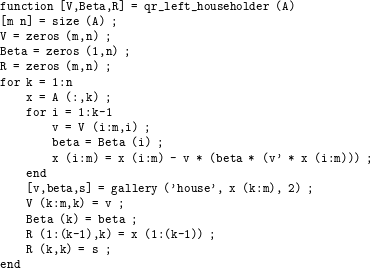
In the sparse case, the for i=1:k-1 loop is replaced with a loop across all rows  $i$ for which R(i,k) is non-zero (a traversal of the
 $k$th row subtree). The data structure is very simple since
 $R$ and
 $V$ grow by one column
 $k$ at a time, and once the
 $k$th column is computed for these matrices they do not change dynamically. The sparse vector x holds the
 $k$ column of
 $R$ and
 $V$ in scattered format, and the pattern
 ${\mathcal{V}}_{k}$ of the
 $k$th column of
 $V$ is computed in the symbolic factorization phase.
7.4 Rank-deficient least-squares problems
If  $A$ is rank-deficient, all of the QR factorization methods described so far (row-Givens, and the left- and right-looking variants of the Householder-based methods) can employ Heath’s (Reference Heath1982) method for handling this case. This method is an integral part of row-Givens, as discussed in Section 7.2. Additional methods for rank-deficient problems are considered here. The resulting QR factorization is referred to as a rank-revealing QR. It is always an approximation, but some methods are more approximate than others. In particular, while it is fast and effective for many matrices in practice, Heath’s (Reference Heath1982) method is the least accurate of the methods considered here.
A rank-revealing factorization is essential for finding reliable solutions to ill-posed systems (both pseudo-inverse and basic solutions), constructing null space bases, and computing the rank. The SVD-based pseudo-inverse provides the most accurate results, but it is not suitable for sparse matrices since the singular vectors of a sparse matrix are all non-zero under very modest assumptions. A less accurate method would be to use QR factorization with column pivoting, in which at the  $k$th step the column with the largest norm is permuted to become the
 $k$th column. This method is commonly used for dense matrices, but it too destroys sparsity (although not as badly as the SVD).
Björck (Reference Björck1984) handles rank-deficiency in his method for handling dense rows of  $A$. The dense rows are withheld from the QR factorization, but the sparse submatrix without these dense rows can become rank-deficient. Björck uses Heath’s (Reference Heath1982) method to handle this case by computing an upper trapezoidal factor
 $R$. He then handles the dense rows of
 $A$ by non-orthogonal eliminations and uses them to update the solution to the entire system for all of
 $A$. The sparse least-squares solver in SPARSPAK-B by George and Ng (Reference George and Ng1984a, Reference George and Ng1984b) relies on row-Givens (George and Heath Reference George and Heath1980). It uses Heath’s (Reference Heath1982) method for rank-deficient problems and Björck’s (Reference Björck1984) for handling dense rows.
Bischof and Hansen (Reference Bischof and Hansen1991) consider a rank-revealing QR factorization that restricts the column pivoting in a right-looking method so as not to destroy sparsity. This is followed by a subsequent factorization of the part of  $R$ (in the lower right corner) that may still be rank-deficient.
Ng (Reference Ng1991) starts with the row-Givens method and Heath’s (Reference Heath1982) method for handling rank-deficiency. In the second phase, the tiny diagonal entries of  $R$ (those that fall below the threshold) are used to construct a full-rank underdetermined system, which is solved via another QR factorization.
The multifrontal QR discussed in Section 11.5 can use Heath’s (Reference Heath1982) method. For example, Heath’s method is used in the multifrontal sparse QR used in MATLAB (Davis Reference Davis2011a). Pierce and Lewis (Reference Pierce and Lewis1997) were the first to consider a multifrontal QR factorization method that handles rank-deficient matrices and computes their approximate rank. They start with a conventional sparse QR (multifrontal in this case), and combine it with a condition estimator (Bischof, Lewis and Pierce Reference Bischof, Lewis and Pierce1990). Columns are removed if found to be redundant by this estimator. A second phase treats the columns found to be redundant in the first phase. More details are discussed in Section 11.5.
In contrast, Foster and Davis (Reference Foster and Davis2013) rely on Heath’s simpler method for the first phase. Columns that are found to be redundant are dropped, but the method computes the Frobenius norm of the small errors that occur from this dropping. The dropped columns are permuted to the end of  $R$. The second phase relies on subspace iteration to obtain an accurate estimate of the null space of the lower right corner of
 $R$ (the redundant columns). Their package includes methods for finding the basic solution, an orthonormal null space basis, an approximate pseudo-inverse solution, and a complete orthogonal decomposition.
7.5 Alternatives to QR factorization
QR factorization is the primary method for solving least-squares problems, but not the only one. The methods discussed below can be faster and take less memory, depending on the sparsity pattern of  $A$ and how well-conditioned it is.
The simplest method is to use the normal equations. Finding  $x$ that minimizes the norm
 $\Vert r\Vert$ of the residual
 $r=b-Ax$ can be done by solving the normal equations
 $A^{T}Ax=A^{T}b$ via sparse Cholesky factorization. This fails if
 $A$ is rank-deficient or ill-conditioned, however. The rank-deficient case is considered in Section 7.4. However, it works well for applications for which the matrices are well-conditioned. For example, Google uses the normal equations to solve the least-squares problems via CHOLMOD (Chen et al. Reference Chen, Davis, Hager and Rajamanickam2008) in their non-linear least-squares solver, Ceres. The Ceres package is used to process all photos in Google Street View, Photo Tours, and many other applications.
Duff and Reid (Reference Duff and Reid1976) compare and contrast four different methods for solving full-rank least-squares problems: (1) the normal equations, (2) QR factorization based on Givens rotations or Householder reflections, (3) the augmented system, and (4) the method of Peters and Wilkinson (Reference Peters and Wilkinson1970), which relies on the LU factorization of the rectangular matrix  $A$. The augmented system
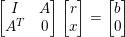 $$\begin{eqnarray}\left[\begin{array}{@{}cc@{}}I & A\\ A^{T} & 0\end{array}\right]\left[\begin{array}{@{}c@{}}r\\ x\end{array}\right]=\left[\begin{array}{@{}c@{}}b\\ 0\end{array}\right]\end{eqnarray}$$
results in a symmetric indefinite matrix for which the multifrontal  $\text{LDL}^{\text{T}}$ factorization is suitable (Section 11). It is not as susceptible to the ill-conditioning of the normal equations. Replacing
 $I$ with a scaled identity matrix
 ${\it\alpha}I$ can improve the conditioning. Peters and Wilkinson (Reference Peters and Wilkinson1970) considered only the dense case, but Duff and Reid (Reference Duff and Reid1976) adapt their method to the sparse case. The method starts with the
 $A=LU$ factorization of the rectangular matrix, followed by the symmetric indefinite factorization
 $L^{T}L=L_{2}D_{2}L_{2}^{T}$. It is just as stable as the augmented system, and can be faster than QR factorization of
 $A$.
Björck and Duff (Reference Björck and Duff1988) extend the method of Peters and Wilkinson (Reference Peters and Wilkinson1970) to the weighted least-squares problem, and present an updating approach for when new rows arrive. The latter is discussed in Section 12.1.
Arioli, Duff and de Rijk (Reference Arioli, Duff and de Rijk1989b) introduce error estimates for the solution of the augmented system that are both accurate and inexpensive to compute. Their results show that the augmented system approach with iterative refinement can be much better, particularly when compared to the normal equations when  $A$ has a dense row. In that case,
 $A^{T}A$ is completely non-zero, which is not the case for the
 $\text{LDL}^{\text{T}}$ factorization of the augmented matrix in (7.1). Results and comparisons with the normal equations are presented by Duff (Reference Duff1990), who shows that the method is stable in practice.
George, Heath and Ng (Reference George, Heath and Ng1983) compare three different methods: (1) the normal equations, (2) the Peters and Wilkinson (Reference Peters and Wilkinson1970) method using MA28 (Duff and Reid Reference Duff and Reid1979b), and (3) the row-Givens method. They conclude that the normal equations are superior when  $A$ is well-conditioned. The method is faster and generates results with adequate accuracy. They find the method of Peters and Wilkinson (Reference Peters and Wilkinson1970) to be only slightly more accurate. They note that the LU factorization of
 $L^{T}L$ takes about the same space as the Cholesky factorization of
 $A^{T}A$. The row-Givens method is robust, being able to solve all of the least-squares problems they consider.
Cardenal, Duff and Jiménez (Reference Cardenal, Duff and Jiménez1998) consider both the least-squares problem for solving overdetermined systems of equations, and the minimum 2-norm problem for undetermined systems. They rely on LU factorization of a different augmented system to (7.1). For overdetermined systems, they solve the system
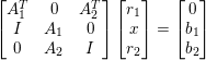 $$\begin{eqnarray}\left[\begin{array}{@{}ccc@{}}A_{1}^{T} & 0 & A_{2}^{T}\\ I & A_{1} & 0\\ 0 & A_{2} & I\end{array}\right]\left[\begin{array}{@{}c@{}}r_{1}\\ x\\ r_{2}\end{array}\right]=\left[\begin{array}{@{}c@{}}0\\ b_{1}\\ b_{2}\end{array}\right]\end{eqnarray}$$
via LU factorization, where  $A_{1}$ is a square submatrix of
 $A$ and
 $A_{2}$ is the rest of
 $A$. This is followed by a solution of
 $A_{1}x=b_{1}J^{T}r_{2}$, where
 $J$ is the (3,2) block in the factor
 $L$ of the 3
 $\times$ 3 block coefficient matrix in (7.2). A related system with the same coefficient matrix but different right-hand side is used to find the minimum 2-norm solution for under-determined systems. Unlike Peters and Wilkinson’s (Reference Peters and Wilkinson1970) method, their method does not require a subsequent factorization of
 $L^{T}L$. They show that the method works well when
 $A$ is roughly square.
Heath (Reference Heath1984) surveys the many methods for solving sparse linear least-squares problems: normal equations, Björck and Duff’s (Reference Björck and Duff1988) method using LU factorization, Gram–Schmidt, Householder reflections (right-looking), Givens rotations (row-Givens), and iterative methods (in particular, LSQR: see Paige and Saunders Reference Paige and Saunders1982). His conclusions are in agreement with the results summarized above. Namely, the normal equations can work well if  $A$ is well-conditioned, and LU factorization is best when the matrix is nearly square, and row-Givens is superior otherwise. Heath concludes that Givens rotations are superior to a right-looking Householder method, but he does not consider the successor to right-looking Householder: the multifrontal QR, which was developed later. Iterative methods such as LSQR are outside the scope of this survey, but Heath states that they can work well, although a preconditioner must be chosen correctly if the matrix is ill-conditioned.
8 Fill-reducing orderings
The fill-minimization problem can be stated as follows. Given a matrix  $A$, find a row and column permutation
 $P$and
 $Q$(with the added constraint that
 $Q=P^{T}$for a sparse Cholesky factorization) such that the number of non-zeros in the factorization of
 $PAQ$, or the amount of work required to compute it, are minimized. While some of these orderings were originally developed for minimizing fill, there are other variants and usage in different contexts such as minimizing flops or exposing parallelism for parallel factorizations.
Section 8.1 discusses the difficulty of the fill-minimization problem, and why heuristics are used. Each following subsection then considers different variations of the problem and algorithms for solving them. Moving entries close to the diagonal is the goal of the profile orderings discussed in Section 8.2. The Markowitz method for finding pivots during LU factorization has already been discussed in Section 6.4, but the method can also be used as a symbolic pre-ordering, as discussed in Section 8.3. Section 8.4 presents the symmetric minimum degree method and its variants, including minimum deficiency, for sparse Cholesky factorization and for other factorizations that can assume a symmetric non-zero pattern. The unsymmetric analogue of minimum degree is considered in Section 8.5, which is suitable for QR or LU factorization with arbitrary partial pivoting. Up to this point, all of the methods considered are local greedy heuristics. Section 8.6 presents nested dissection, a completely different approach that uses graph partitioning to break the problem into subgraphs that are ordered independently, typically recursively. This method is well-suited to parallel factorizations, particularly matrices arising from discretizations of two- and three-dimensional problems. Section 8.7 considers the block triangular form and other special forms. Finally, pre-orderings based on independent sets, and elimination tree rotations, are discussed in Section 8.8. These methods take an alternative approach to finding orderings suitable for parallel factorizations.
8.1 An NP-hard problem
Computing an ordering for the minimum fill is NP-hard, in its many forms. Rose and Tarjan (Reference Rose and Tarjan1978) showed that computing the minimum elimination order is NP-complete for directed graphs and described how to compute the fill-in for any ordering (symbolic analysis). Gilbert (Reference Gilbert1980) made corrections to the proofs of Rose and Tarjan (Reference Rose and Tarjan1978). As a result, both of these works should be considered together while reading. Rose et al. (Reference Rose, Tarjan and Lueker1976) conjectured that it is also true that minimum fill is NP-hard for undirected graphs, which was later proved to be correct (Yannakakis Reference Yannakakis1981). Recently, Luce and Ng (Reference Luce and Ng2014) showed that the minimum flops problem is NP-hard for the sparse Cholesky factorization, and it is different from the minimum fill problem. Peyton (Reference Peyton2001) introduced an approach to begin with any initial ordering and refine it to a minimal ordering. One implementation of such a method is described by Heggernes and Peyton (Reference Heggernes and Peyton2008). Such approaches are useful when the initial ordering is not minimal. The rest of this section considers orderings to reduce the fill and points out other variants or usage when appropriate.
8.2 Profile, envelope, wavefront, and bandwidth reduction orderings
Given a sparse symmetric matrix  $A$ of size
 $n\times n$ with non-zero diagonal elements, we will consider the lower triangular portion of
 $A$ for the following definitions. Let
 $f_{i}(A)$ be the first non-zero entry in the
 $i$th row of
 $A$ or
 $$\begin{eqnarray}f_{i}(A)=\min \{j:1\leq j\leq i,\text{with}~a_{ij}\neq 0\}.\end{eqnarray}$$
The bandwidth of  $A$ is
 $$\begin{eqnarray}\max \{i-f_{i}(A),1\leq i\leq n\}.\end{eqnarray}$$
The envelope of  $A$ is
 $$\begin{eqnarray}\{(i,j):1\leq i\leq n,f_{i}(A)\leq j<i\}.\end{eqnarray}$$
The profile of the matrix is the number of entries in the envelope in addition to the number of entries in the diagonal. In the frontal method (discussed in Section 10) the matrix  $A$ is never fully assembled. Instead the assembly and elimination phases are interleaved with each other. In order to get better performance, the number of equations active at any stage of the elimination process needs to be minimized. Equation
 $j$ is called active if
 $j\geq i$ and there is a non-zero entry in column
 $j$ with row index
 $k$ such that
 $k\geq i$. If
 $w_{i}$ denotes the number of equations that are active during the
 $i$th step of the elimination, the maximum wavefront and mean-square wavefront are defined, respectively, as
 $$\begin{eqnarray}\displaystyle & \displaystyle \max _{1\leq i\leq n}\{w_{i}\}, & \displaystyle\end{eqnarray}$$
 $$\begin{eqnarray}\displaystyle & \displaystyle \frac{1}{n}\mathop{\sum }_{i=1}^{n}|w_{i}|^{2}. & \displaystyle\end{eqnarray}$$
In frontal methods, the maximum wavefront affects the storage, and the root-mean-square wavefront affects the work, as the work in eliminating a variable is proportional to the square of the active variables. Methods that reduce the maximum wavefront or mean-square wavefront overlap considerably with methods to reduce the bandwidth, envelope or profile. This subsection covers these approaches together.
The problem of minimizing the bandwidth is NP-complete (Papadimitriou Reference Papadimitriou1976). Tewarson (Reference Tewarson1967b) presents two methods for reducing the lower bandwidth only, so that the matrix is permuted into a mostly upper triangular form. Among the methods described here, a variation of the CM method originally proposed by Cuthill and McKee (Reference Cuthill and Mckee1969) is one of the more popular methods even now. Cuthill and McKee (Reference Cuthill and Mckee1969) describe a method for minimizing the bandwidth. Their method uses the graph of  $A$ and starts with a vertex of minimum degree and orders it as the first vertex. The nodes adjacent to this vertex (called level 1) are numbered next in order of increasing degree. This procedure is repeated for each node in the current level until all vertices are numbered. Later, George (Reference George1971) proposed reversing the ordering obtained from the Cuthill–McKee method, which resulted in better orderings. This change to the original method is called the reverse Cuthill–McKee ordering, or RCM. King (Reference King1970) proposed a method to improve the frontal methods with a wavefront reduction algorithm. Levy’s (Reference Levy1971) algorithm for wavefront reduction is similar to King’s algorithm where all vertices at each stage are considered instead of unlabelled vertices adjacent to already labelled vertices. Cuthill (Reference Cuthill, Rose and Willoughby1972) compares the original method of Cuthill and McKee (Reference Cuthill and Mckee1969) with this reversed ordering and King’s method for a number of metrics such as bandwidth, wavefront and profile reduction. The results showed that the Cuthill–McKee method and its reverse gave smaller bandwidths; Levy’s algorithm gave smaller wavefronts and profiles. Other methods that followed used iterations to improve the ordering further (Collins Reference Collins1973) or expensive schemes to find different starting vertices (Cheng Reference Cheng1973a, Reference Cheng1973b). The RCM and CM methods both result in similar bandwidth. However, RCM also results in a smaller envelope (Liu and Sherman Reference Liu and Sherman1976). A linear implementation of the RCM method is possible by being careful in the sorting step (Chan and George Reference Chan and George1980).
A faster algorithm to compute the ordering was proposed by Gibbs, Poole and Stockmeyer (Reference Gibbs, Poole and Stockmeyer1976a) for bandwidth and profile reduction. The GPS algorithm finds pseudo-peripheral vertices iteratively and then tries to improve the width of a level. In addition it uses a reverse numbering scheme. Later work compared this new method to a number of other algorithms discussed above (Gibbs, Poole and Stockmeyer Reference Gibbs, Poole and Stockmeyer1976b). The results showed that both RCM and GPS are good bandwidth reduction algorithms and GPS is substantially faster. King’s algorithm results in a better profile when it does well, but RCM and GPS are more consistent for profile reduction. In terms of profile reduction, Snay’s (Reference Snay1969) algorithm resulted in better profile than RCM. One of the earliest software packages to implement bandwidth and profile reduction, called REDUCE (Crane, Gibbs, Poole and Stockmeyer Reference Crane, Gibbs, Poole and Stockmeyer1976), implements the GPS algorithm (Gibbs et al. Reference Gibbs, Poole and Stockmeyer1976a). Gibbs (Reference Gibbs1976) also proposed a hybrid algorithm by using the GPS technique with King’s algorithm, to arrive at a profile reduction algorithm that is more robust than King’s algorithm. This hybrid algorithm arrives at level sets starting from pseudo-peripheral vertices and uses King’s algorithm for the numbering within the level.
George (Reference George and Barker1977b) compares RCM with nested dissection (discussed in Section 8.6 below) based on the operation count and memory usage for the sparse Cholesky factorization, and the time to compute the orderings. His results show that the solvers match earlier complexity analysis. George also proposed in this paper a one-way nested dissection scheme where the separators are found in the same dimension. One-way nested dissection gives a slight advantage in the solve time, but nested dissection is substantially better in factorization times. Everstine (Reference Everstine1979) compares RCM, GPS, and Levy’s algorithm on different metrics, and established that GPS is good for both maximum wavefront and profile reduction.
Brown and Wait (Reference Brown, Wait and Duff1981) present a variation of RCM that accounts for irregular structures in the graph, such as holes in a finite element mesh. In this case, RCM can oscillate between two sides of a hole in the mesh, first ordering one side and then the other, and back again. Brown and Wait avoid this by ordering all of the unordered neighbours of a newly ordered node in a group, rather than strictly in the order of increasing degree.
Lewis (Reference Lewis1982a, Reference Lewis1982b) describes strategies to improve both GPS and the algorithm of Gibbs (Reference Gibbs1976) and practical implementation of both these algorithms as a successor of the REDUCE software. Linear-time implementations of these profile reduction algorithms, such as Levy, King and Gibb’s algorithms, are possible by efficient implementation of search sets to minimize fronts (Marro Reference Marro1986). While these strategies result in good implementations, Sloan (Reference Sloan1986) presented a simple profile and wavefront reduction algorithm that is faster than all these other implementations. The method introduces two changes to finding pseudo-peripheral vertices. First, the focus is on low degree nodes in the last level. Second, the short-circuiting strategy introduced by George and Liu (Reference George and Liu1979b) is used as well.
Hager (Reference Hager2002) introduces a sequence of row and column and exchanges to minimize the profile. These methods are useful for refining other orderings. An implementation of this approach without big penalties on runtime is also possible (Reid and Scott Reference Reid and Scott2002).
Spectral methods do not use level structures. Instead, spectral algorithms for envelope reduction use the eigenvector corresponding to the smallest positive eigenvalue of the Laplacian matrix corresponding to a given matrix (Barnard, Pothen and Simon Reference Barnard, Pothen and Simon1995). Analysis of this method shows that despite the high cost of these methods, they result in better envelope reductions (George and Pothen Reference George and Pothen1997). These methods have the advantage of easy vectorization and parallelization. George and Pothen propose the idea for a multilevel algorithm to compute the eigenvector. Boman and Hendrickson (Reference Boman and Hendrickson1996) described an implementation of these ideas in a multilevel framework in the Chaco library (Hendrickson and Leland Reference Hendrickson and Leland1995a). A hybrid algorithm that combines the spectral method for envelope and wavefront reduction with a refinement step that uses Sloan’s algorithm improves the wavefront at the cost of time (Kumfert and Pothen Reference Kumfert and Pothen1997). They also show a time-efficient implementation of Sloan’s algorithm for large problems. These changes are also considered in the context of the MC60 and MC61 codes (Reid and Scott Reference Reid and Scott1999). Grimes, Pierce and Simon (Reference Grimes, Pierce and Simon1990) proposed finding pseudo-peripheral vertices via a spectral methods for a regular access pattern in an out-of-the-core implementation.
A number of the ordering schemes for frontal methods need to differentiate between element numbering and nodal numbering in the finite element mesh. Bykat (Reference Bykat1977) proposed an RCM-like method to do element numbering by defining an element graph, where the vertices are elements and the edges signify adjacent elements that share an edge. The Cuthill–McKee method is used on this element graph. Razzaque (Reference Razzaque1980) discusses an indirect scheme to reduce the frontwidth or the wavefront for a frontal method. It uses the band reduction method on the nodes of the mesh and then numbers the elements based on the ordering of the nodes that the elements correspond to. Other methods follow this pattern as well by using different algorithms for nodal numbering (Ong Reference Ong1987). The direct numbering schemes such as that proposed by Pina (Reference Pina1981) attempt to find the best element numbering to reduce the frontwidth in each step by considering nodes with minimum degree and the corresponding elements. Fenves and Law (Reference Fenves and Law1983) describe a two-step scheme where the elements are ordered with RCM and the nodes are numbered locally, which results in better fill than just doing RCM on the nodes. Local ordering in this method is based on the number of elements a node is incident upon, and the element graph uses adjacencies in more than two dimensions.
There are other methods (Hoit and Wilson Reference Hoit and Wilson1983, Silvester, Auda and Stone Reference Silvester, Auda and Stone1984, Webb and Froncioni Reference Webb and Froncioni1986) that use nodal and/or element numberings to minimize the frontwidth. A comparison of these direct and indirect methods for wavefront minimization show similar performance (Duff, Reid and Scott Reference Duff, Reid and Scott1989b). In these comparisons Sloan’s ordering is used to order indirectly, and a more aggressive short-circuiting than used by George and Liu (Reference George and Liu1979b) is used here. De Souza, Keunings, Wolsey and Zone (Reference De Souza, Keunings, Wolsey and Zone1994) approach the frontwidth problem by using a graph partitioning-like approach that results in better frontwidth. It is also possible to use a hybrid method of spectral ordering and Sloan’s algorithm for a frontal solver (Scott Reference Scott1999b). This approach follows the work of Reid and Scott (Reference Reid and Scott1999) and Kumfert and Pothen (Reference Kumfert and Pothen1997). When the matrices are highly unsymmetric the row graph is used with a modified Sloan’s algorithm for an effective strategy for frontal solvers (Scott Reference Scott1999a). Reid and Scott (Reference Reid and Scott2001) also analyse the effect of reversing the row ordering for frontal solvers. More theoretical approaches for bandwidth minimization have been considered, where they propose exact solutions for small problems (Del Corso and Manzini Reference Del Corso and Manzini1999).
8.3 Symbolic Markowitz
Right-looking methods for LU factorization using the Markowitz (Reference Markowitz1957) method and its variants typically find the pivots during numerical factorization. In this section, we discuss methods that use this strategy to pre-order the matrix prior to numerical factorization.
Markowitz’s method is a local heuristic to choose the pivot at the  $k$th step. Let
 $r_{i}^{k}$ and
 $c_{j}^{k}$ be the number of non-zero entries in row
 $i$ and column
 $j$, respectively, in the
 $(n-k)\times (n-k)$ submatrix yet to be factored after the
 $k$th step. The Markowitz algorithm then greedily picks the non-zero entry
 $a_{ij}^{k}$ in the remaining submatrix that has the minimum Markowitz count, which is the product of the non-zeros left in the rows and columns
 $(r_{i}^{k}-1)\times (c_{j}^{k}-1)$. This strategy has been successfully used for quite some time, in different factorizations with different variations.
The work of Norin and Pottle (Reference Norin and Pottle1971) is one of the early examples considering a metric with weighted schemes that can be adjusted to a Markowitz-like metric. The weights can also be adjusted to use other metrics such as the row or column degree for ordering.
Markowitz ordering has been used more recently for symmetric permutation of unsymmetric matrices, permuting the diagonal entries (Amestoy, Li and Ng Reference Amestoy, Li and Ng2007a). Such a method is purely symbolic, and allows the use of the non-symmetric structure of the matrices without resorting to some form of symmetrization. Amestoy et al. (Reference Amestoy, Li and Ng2007a) show that this can be done efficiently in terms of time and memory using techniques such as local symmetrization. This work was later extended to consider the numerical values of the matrix by introducing a hybrid method that uses a combination of structure and values to pick the pivot (Amestoy, Li and Pralet Reference Amestoy, Li and Pralet2007b). The new method does not limit the pivot to just the diagonal entries, but it uses a constraint matrix that uses both structural and numerical information to control how pivots are chosen.
8.4 Symmetric minimum degree and its variants
The minimum degree algorithm is a widely used heuristic for finding a permutation  $P$ so that
 $PAP^{T}$ has fewer non-zeros in its factorization than
 $A$. It is a greedy method that selects the sparsest pivot row and column during the course of a right-looking sparse Cholesky factorization. Minimum degree is a local greedy strategy, or a ‘bottom-up’ approach, since it finds the leaves of the elimination tree first. Tinney and Walker (Reference Tinney and Walker1967) developed the first minimum degree method for symmetric matrices. Note that the word ‘optimal’ in the title of their paper is a misnomer, since minimum degree is a non-optimal yet powerful heuristic for an NP-hard problem (Yannakakis Reference Yannakakis1981).
Its basic form is a simple extension of Algorithm 4.2 presented in Section 4.3. At each step of an right-looking elimination, one pivot is removed and its update is applied to the lower right submatrix. This is the same as removing a node from the graph and adding edges to its neighbours so that they become a clique. The minimum degree ordering algorithm simply selects as pivot a node of least degree, rather than eliminating them in their original order (as is done by Algorithm 4.2).
There are many variants of this local greedy heuristic. Rose (Reference Rose and Read1972) surveyed a wide range of methods and criteria, including minimum degree and minimum deficiency (in which a node that causes the least amount of new fill-in edges is selected), and other related methods.
8.4.1 Minimum degree
In this section, we consider the evolution of the primary variant, which is the symmetric minimum degree method.
The first reported efficient implementation was by George and McIntyre (Reference George and Mcintyre1978), who also adapted the method to exploit the natural cliques that arise in a finite element discretization. Each finite element is a clique of a set of nodes, and they distinguish two kinds of nodes: those whose neighbours lie solely in their own clique/element (interior nodes), and those with some neighbours in other cliques/elements. Interior nodes cause no fill-in, and can be eliminated as soon as any other node in an element is eliminated.
Huang and Wing (Reference Huang and Wing1979) present a variation of minimum degree that also considers the number of parallel factorizations steps. The node with the lowest metric is selected, where the metric is a weighted sum of the operation count (roughly the square of the degree) and the depth. The depth of a node is the earliest time it can be ready to factorize in a parallel elimination method.
The use of quotient graphs for symbolic factorization is described in Algorithm 4.3 in Section 4.3. George and Liu (Reference George and Liu1980a) introduce these graphs to speed up the minimum degree algorithm. This greatly reduces the storage requirements. A quotient graph consists of two kinds of nodes: uneliminated nodes, which correspond to original nodes of the graph of  $A$, and eliminated nodes, which correspond to the new elements formed during elimination. The quotient graph is represented in adjacency list form. Each regular node
 $j$ has two lists:
 ${\mathcal{A}}_{j}$, the set of nodes adjacent to
 $j$, and
 ${\mathcal{E}}_{j}$, the set of elements adjacent to
 $j$. Each element
 $j$ corresponds to a column of the factor
 $L$, and thus has a single list
 ${\mathcal{L}}_{j}$ of regular nodes. As soon as node
 $j$ is selected as a pivot, the new element is formed,
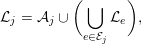 $$\begin{eqnarray}{\mathcal{L}}_{j}={\mathcal{A}}_{j}\cup \biggl(\mathop{\bigcup }_{e\in {\mathcal{E}}_{j}}{\mathcal{L}}_{e}\biggr),\end{eqnarray}$$
and all prior elements in  ${\mathcal{E}}_{j}$ are deleted. This pruning allows the quotient graph to be represented in-place, in the same memory space as
 $A$, even though it is a dynamically changing graph.
The next node selected is the one of least degree, which is the node with the smallest set size as given by (8.6). This information is not in the quotient graph, and thus when node  $j$ is eliminated, the degree of all the nodes
 $i$ adjacent to
 $j$ must be recomputed by computing the set union (8.6) for each node
 $i$. This is the most costly step of the method, and a great deal of subsequent algorithmic development has gone into reducing this work.
George and Liu (Reference George and Liu1980b) simplify the data structures even further by using reachable sets instead of the quotient graph to model the graph elimination. In this method, the graph of the matrix does not change at all. Instead, the degrees of the as yet uneliminated nodes are computing by a wider scan of the graph, to compute the reach of each node via prior eliminated nodes. This search is even more costly than the degree update (8.6), however.
One approach to reducing the cost is to reduce the number of times the degree of a node must be recomputed. Liu (Reference Liu1985) introduces the idea of multiple minimum degree (MMD, a function in SPARSPAK: George and Liu Reference George and Liu1979a). In this method, a set of independent nodes is chosen, all of the same least degree, but none of which are adjacent to each other. Next, the degrees of all their uneliminated neighbours are computed. If an uneliminated node is adjacent to multiple eliminated nodes, its degree must be only computed once, not many times. Other implementations of the minimum degree algorithm include YSMP (Eisenstat, Gursky, Schultz and Sherman Reference Eisenstat, Gursky, Schultz and Sherman1982, Eisenstat, Schultz and Sherman Reference Eisenstat, Schultz and Sherman1981), MA27 (Duff et al. Reference Duff, Erisman and Reid1986, Duff and Reid Reference Duff and Reid1983a), and AMD (Amestoy et al. Reference Amestoy, Davis and Duff1996a)).
Minimum degree works well for many matrices, but nested dissection often works better for matrices arising from two- or three-dimensional discretizations. Liu (Reference Liu1989b) shows how to combine the two methods. Nested dissection is used only partially, to obtain a partial order. This provides constraints for the minimum degree algorithm; all nodes within a given constraint set are ordered before going on to the next set. The CAMD package in SuiteSparse (see Section 13) provides an implementation of this method.
George and Liu (Reference George and Liu1989) survey the evolution of the minimum degree algorithm and the techniques used to improve it, namely the quotient graph, indistinguishable nodes, mass elimination, multiple elimination, and external degree. Two nodes that take on the same adjacency structure will remain that way until one is eliminated, at which point the other will be a node of least degree and can be eliminated immediately without causing any further fill-in. Thus, these indistinguishable nodes can be merged, and further merging can be done with more nodes as they are discovered. The edges between nodes inside a set of indistinguishable nodes do not contribute to any fill-in (the set is already a clique), and the external degree takes this into account, to improve the ordering quality. Indistinguishable nodes can also be found prior to starting the ordering, further reducing the ordering time and improving ordering quality (Ashcraft Reference Ashcraft1995). Mass elimination occurs if a node adjacent to the pivot node  $j$ has only a single edge to the new element
 $j$; rather than updating its degree, this node can be eliminated immediately with no fill-in.
Since the graph changes dynamically and often unpredictably during elimination, very little theoretical work has been done on the quality of the minimum degree ordering for irregular graphs. Berman and Schnitger (Reference Berman and Schnitger1990) provide asymptotic bounds for the fill-in with regular graphs (two-dimensional toruses), when a specific tie-breaking strategy is used for the common case that occurs when more than one node has least degree. Even though little is known about any guarantee of ordering quality in the general case, the method works well in practice. Berry, Dahlhaus, Heggernes and Simonet (Reference Berry, Dahlhaus, Heggernes and Simonet2008) relate the minimum degree algorithm to the problem of finding minimal triangulations, and in so doing give a partial theoretical explanation for the ordering quality of the method.
Since computing the exact degree is costly, Amestoy et al. (Reference Amestoy, Davis and Duff1996a, Reference Amestoy, Davis and Duff2004a) developed an approximate minimum degree ordering (AMD). The idea derives from the rectangular frontal matrices in UMFPACK, and was first developed in that context (Davis and Duff Reference Davis and Duff1997), discussed in Section 11.4. Consider the exact degree of node  $i$ after node
 $j$ has been eliminated:
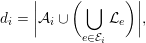 $$\begin{eqnarray}d_{i}=\biggl|{\mathcal{A}}_{i}\cup \biggl(\mathop{\bigcup }_{e\in {\mathcal{E}}_{i}}{\mathcal{L}}_{e}\biggr)\biggr|,\end{eqnarray}$$
where  $j\in {\mathcal{E}}_{i}$ is the new pivotal element. The time to compute this degree is the sum of the set sizes, which is higher than
 $O(d_{i})$. The external degree is normally used, but equation (8.7) is simpler for the purpose of this discussion. Note that for both the exact and approximate degrees, when the metric is computed,
 ${\mathcal{A}}_{i}$ is pruned of all nodes in the pattern of the pivot element,
 ${\mathcal{L}}_{j}$. AMD replaces the exact degree with an upper bound,
 $$\begin{eqnarray}\overline{d}_{i}=|{\mathcal{A}}_{i}|+|{\mathcal{L}}_{j}|+\mathop{\sum }_{e\in {\mathcal{E}}_{i}\setminus j}|{\mathcal{L}}_{e}\setminus {\mathcal{L}}_{p}|.\end{eqnarray}$$
The set differences are found in a first pass, the bound is computed in a second pass, and the amortized time to compute (8.8) is only  $O(|{\mathcal{A}}_{i}|+|{\mathcal{E}}_{i}|)$. This is far less than the time required to compute (8.7).
Liu (Reference Liu1989b) created a hybrid between nested dissection and the exact minimum degree method (MMD). Pellegrini, Roman and Amestoy (Reference Pellegrini, Roman and Amestoy2000) take this approach one step further by forming a tighter coupling between nested dissection and a halo approximate minimum degree method. Nested dissection breaks the graph into subgraphs, which are ordered with a variation of AMD that takes into account the boundaries (halo) between the subgraphs.
8.4.2 Minimum deficiency
Minimum degree is the dominant local greedy heuristic for sparse direct methods, but other heuristics have been explored. Selecting a node of minimum degree  $d$ provides a bound on the number of new edges (fill-in) that can appear in the graph (
 $(d^{2}-d)/2$). Another approach is to simply pick the node that causes the least fill-in. This method gives somewhat better orderings in general, but it is very costly to implement, in terms of runtime.
The method was first considered by Berry (Reference Berry1971). Nakhla, Singhal and Vlach (Reference Nakhla, Singhal and Vlach1974) added a tie-breaking method; if two nodes cause the same fill-in, then the node of least degree is selected. Both methods are very costly, and thus little work was done in this method until Rothberg and Eisenstat’s (Reference Rothberg and Eisenstat1998) work.
The approximate degree introduced by Amestoy et al. (Reference Amestoy, Davis and Duff1996a) spurred the search for approximations to the deficiency, which are faster to compute than the exact deficiency and yet which retain some of the ordering quality of the exact deficiency. Rothberg and Eisenstat (Reference Rothberg and Eisenstat1998) consider three algorithms: approximate minimum mean local fill (AMMF), approximate minimum increase in neighbour degree (AMIND), and several variants of approximate minimum full. Their first method (AMMF) is an enhancement to the minimum degree method, to obtain a cheap upper bound on the fill-in. If the degree of node  $i$ is
 $d$, and if
 $c=|{\mathcal{L}}_{j}|$ is the size of the most recently created pivotal element that contains
 $i$, then
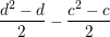 $$\begin{eqnarray}\frac{d^{2}-d}{2}-\frac{c^{2}-c}{2}\end{eqnarray}$$
is an upper bound on the fill-in, since eliminating  $i$ will not create edges inside the prior clique
 $j$. This metric is modified when considering a set of
 $k$ indistinguishable nodes, by dividing the bound by
 $k$, to obtain the AMMF heuristic. The AMIND heuristic modifies the AMMF metric by subtracting
 $dk$, which would be the aggregate change in the degree of all neighbouring nodes if node
 $i$ is selected as the next pivot. They conclude that the exact minimum deficiency provides the best quality, although it is prohibitively expensive to use. Their most practical method (AMMF) cuts flop counts by about 25% over AMD, at a cost of about the same increase in runtime to compute the ordering.
Ng and Raghavan (Reference Ng and Raghavan1999) present two additional heuristics: a modified minimum deficiency (MMDF) and a modified multiple minimum degree (MMMD). MMDF exploits the set differences found by AMD,  $|{\mathcal{L}}_{e}\setminus {\mathcal{L}}_{p}|$, for all prior pivotal elements
 $e\in {\mathcal{E}}_{i}$. This set difference defines a subset of a clique, and if node
 $i$ is eliminated, no fill-in will occur with these partial cliques. If the partial cliques are disjoint, their effects can be combined by subtracting them from the upper bound on fill-in that would occur if
 $i$ were to be selected as a pivot. The method adds an approximate correction term to account for the fact that the partial cliques might not be disjoint. The MMDF heuristic accounts for all adjacent partial cliques, whereas MMMD tries to take into account only the largest one. Reiszig (Reference Reiszig2007) presents a modification to MMDF that gives a tighter bound on the fill-in, and presents performance results of his implementation of this method and those of Rothberg and Eisenstat (Reference Rothberg and Eisenstat1998) and Ng and Raghavan (Reference Ng and Raghavan1999).
8.5 Unsymmetric minimum degree
The previous section considered the symmetric ordering problem via minimum degree and other related local greedy heuristics. In this section we consider related heuristics for finding pre-orderings  $P_{r}$ and
 $P_{c}$ for an unsymmetric or rectangular matrix
 $A$, so that the fill-in in the LU or QR factorization of the permuted matrix
 $P_{r}AP_{c}$ has less fill-in that that of
 $A$. The two kinds of factorizations are very closely related, as discussed in Section 6.1, since the non-zero pattern of the QR factorization provides an upper bound on the non-zero pattern of the LU factorization, assuming worst-case pivoting for the latter. As a result, all of the methods in the papers discussed here apply nearly equally for both QR and LU factorization, since the column orderings they compute can be directly used for the LU factorization of
 $P_{r}AP_{c}$, where
 $P_{r}$ is found via partial pivoting, or for the QR factorization of
 $AP_{c}$.
Row and column orderings that are found during the numerical phase of row-Givens QR factorization have already been discussed in Section 7.2, namely, those of Duff (Reference Duff1974b), Gentleman (Reference Gentleman and Watson1975), Zlatev (Reference Zlatev1982), Ostrouchov (Reference Ostrouchov1993), and Robey and Sulsky (Reference Robey and Sulsky1994). George and Ng (Reference George and Ng1983) and George, Liu and Ng (Reference George, Liu and Ng1984b, Reference George, Liu and Ng1986b, Reference George, Liu and Ng1986c) consider row pre-orderings based on a nested dissection approach; these methods are discussed in Section 8.6.2.
The symmetric and unsymmetric ordering methods are closely related. Assuming the matrix  $A$ is strong-Hall, the non-zero pattern of the Cholesky factor
 $L$ of
 $A^{T}A$ is the same as the factor
 $R$ for QR factorization, as discussed in Section 7.1. Thus, finding a symmetric permutation
 $P$ to reduce fill-in in the Cholesky factorization of symmetric matrix
 $(AP)^{T}AP$ will also be a good method for finding a column permutation
 $P$ for the QR factorization of
 $AP$. Tewarson (Reference Tewarson1967c) introduced the graph of
 $A^{T}A$ for ordering the columns of
 $A$ prior to LU factorization, as the column intersection graph of
 $A$.
The difficulty with this approach is that it requires  $A^{T}A$ to be formed first. This matrix can be quite dense. A single dense row causes
 $A^{T}A$ to become completely non-zero, for example. If this is the case, the
 $R$ factor for QR factorization will be dense if
 $A$ is strong-Hall, but it can be very sparse otherwise. Also, the LU factorization of
 $A$ can have far fewer non-zeros than
 $A^{T}A$, even if
 $A$ as a dense row. To avoid forming
 $A^{T}A$, two related algorithms, COLMMD (Gilbert et al. Reference Gilbert, Moler and Schreiber1992) and COLAMD (Davis, Gilbert, Larimore and Ng Reference Davis, Gilbert, Larimore and Ng2004b, Reference Davis, Gilbert, Larimore and Ng2004a) operate on the pattern of
 $A$ instead, while implicitly ordering the matrix
 $A^{T}A$.
The key observation is that every row of  $A$ creates a clique in the graph of
 $A^{T}A$. The matrix product
 $A^{T}A$ can be written as the sum of outer products,
 $\sum a_{i}^{T}a_{i}$, for each row
 $i$. Suppose row 1 has non-zeros in columns 5, 7, 11, and 42. In this case,
 $a_{1}^{T}a_{1}$ is a matrix that is non-zero except for entries residing in rows 5, 7, 11, and 42, and in the same columns. That is, the graph of
 $a_{1}^{T}a_{1}$ is a clique of these four nodes. As a result, the matrix
 $A$ can be viewed as already forming a quotient graph representation of
 $A^{T}A$: each row of
 $A$ is a single element (clique), and each column of
 $A$ is a node.
The minimum degree ordering method would then select a pivot node (column)  $j$ with least degree, and eliminate it. After elimination, a new element is formed, which is the union of all rows
 $i$ that contain a non-zero in column
 $j$. Any such rows (either original rows, or prior pivotal elements) used to form this set union are now subsets of this new element, and can thus be discarded without losing any information in the pattern of the reduced submatrix. These rows are merged into the new element.
This elimination process can be used to model either QR factorization, or LU factorization where the pivot row is assumed to take on the non-zero pattern of all candidate pivot rows.
Let  ${\mathcal{A}}_{i}$ denote the original row
 $i$ of
 $A$, and let
 ${\mathcal{R}}_{k}$ denote the pivotal row formed at step
 $k$. Let
 ${\mathcal{C}}_{j}$ represent column
 $j$ as a list of original row indices
 $i$ and new pivotal elements
 $e$. This list is analogous to the
 ${\mathcal{E}}_{j}$ lists in the quotient graph used for the symmetric minimum degree algorithm. At the
 $k$th step,
 ${\mathcal{R}}_{k}$ is constructed as follows, if we assume no column permutations:
 $$\begin{eqnarray}{\mathcal{R}}_{k}=\biggl(\mathop{\bigcup }_{e\in {\mathcal{C}}_{k}}{\mathcal{R}}_{e}\biggr)\cup \biggl(\mathop{\bigcup }_{i\in {\mathcal{C}}_{k}}{\mathcal{A}}_{i}\biggr)\setminus \{k\}.\end{eqnarray}$$
After  ${\mathcal{R}}_{k}$ is constructed, the sets
 ${\mathcal{R}}_{e}$ and
 ${\mathcal{A}}_{i}$ are redundant, and thus deleted. This deletion can be modelled with the row-merge tree, shown in Figure 8.1, where these prior rows are merged into the pivotal row.
Example of symbolic elimination and the row-merge tree, assuming no column reordering (Davis, Gilbert, Larimore and Ng Reference Davis, Gilbert, Larimore and Ng2004a).
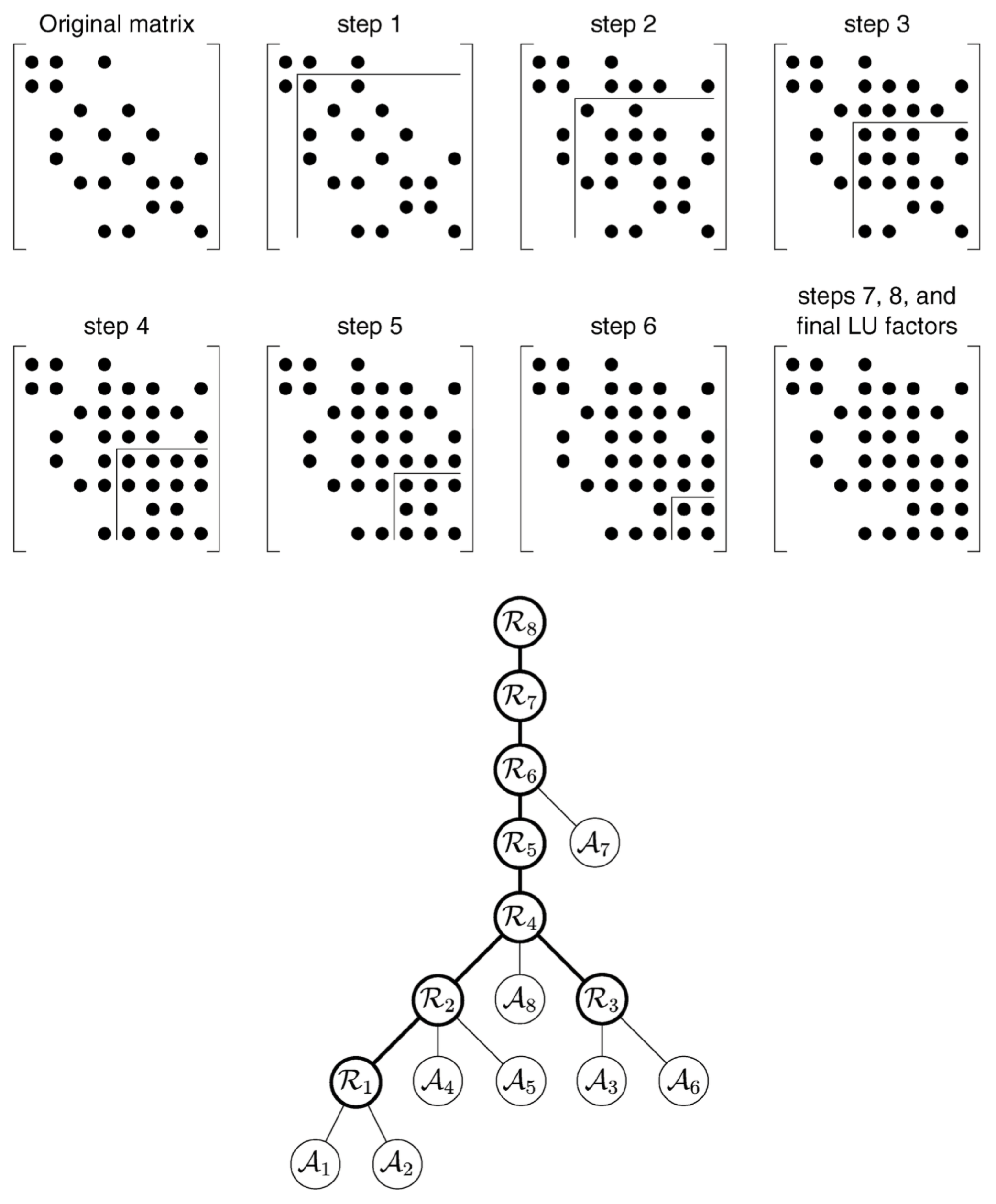
With column pivoting, a different column  $j$ is selected at the
 $k$th step, based on an exact or approximate minimum degree heuristic. The exact degree of a column
 $j$ is
 $|{\mathcal{R}}_{j}|$, which can be computed after each step using (8.9). This is very costly to compute, so approximations are often used. COLMMD uses the sum of the set sizes, as a quick-to-compute upper bound. However, it does not produce as good an ordering as the exact degree, in terms of fill-in and flop count for the subsequent LU or QR factorization. COLAMD relies on the same approximation used in the symmetric AMD algorithm, as a sum of set differences. The COLMMD and COLAMD approximations take the same time to compute (asymptotically) but the latter gives as good an ordering as a method that uses the exact degree. Both COLMMD and COLAMD are available in MATLAB. The latter is also used for
 , and for the sparse LU and QR factorizations (UMFPACK and SuiteSparseQR).
8.6 Nested dissection
8.6.1 Symmetric nested dissection
Nested dissection is a fill-reducing ordering well-suited to matrices arising from the discretization of a problem with two- or three-dimensional geometry. The goal of this ordering is the same as the minimum degree ordering; it is a heuristic for reducing fill-in, not the profile or bandwidth. Consider the undirected graph of a matrix  $A$ with symmetric non-zero pattern. Nested dissection finds a vertex separator that splits the graph into two or more roughly equal-sized subgraphs (left and right), when the vertices in the separator (and their incident edges) are removed from the graph. The subgraphs are then ordered recursively, via nested dissection for a large subgraph or minimum degree for a small one.
With a one-level vertex separator, a matrix is split into the following form, where rows of  $A_{33}$ correspond to the vertices of the separator, rows of
 $A_{11}$ correspond to the vertices in the left subgraph, and rows of
 $A_{22}$ correspond to the vertices in the right subgraph. Since the left subgraph (
 $A_{11}$) and right subgraph (
 $A_{22}$) are not joined by any edges,
 $A_{12}$ is zero:
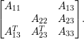 $$\begin{eqnarray}\left[\begin{array}{@{}ccc@{}}A_{11} & & A_{13}\\ & A_{22} & A_{23}\\ A_{13}^{T} & A_{23}^{T} & A_{33}\end{array}\right]\!.\end{eqnarray}$$
There are many methods for finding a good vertex separator. This section surveys these methods from the perspective of sparse direct factorizations. Finding good vertex separators has been traditionally studied in conjunction with edge separators even when one can directly compute the vertex separators. We cover both direct and indirect methods to compute the vertex separators.
Kernighan and Lin (Reference Kernighan and Lin1970) created a heuristic method that starts with an initial assignment of vertices to two parts and iteratively swaps vertices between the two parts of the graph. The method swaps vertices to improve the gain in cut quality, which is the number of edges in the edge cut. In an attempt to escape a local minimum, vertices can be swapped even if the gain is negative. This process continues for many swaps (say, 50), until the method either finds a better cut (a positive gain) or it gives up and retracts back to the best cut found so far. The method has been used for a very long time for partitioning and ordering.
Fiduccia and Mattheyses (Reference Fiduccia and Mattheyses1982) proposed several practical improvements to these methods, especially in steps to find the best vertex to move and update the gain. Like Kernighan–Lin, it continues to make changes for a certain number of steps even with negative gain to avoid any local minima. Local methods such as these are typically used as a refinement step in present-day multilevel methods. The basic step in the algorithm is to move one vertex from one part to the other, in contrast to Kernighan–Lin, which always swaps two vertices.
The nested dissection method, as it was originally proposed, was used to partition finite element meshes with  $n\times n$ elements to reduce the operation count of the factorizations from
 $O(n^{4})$ for the banded orderings to
 $O(n^{3})$ floating-point operations with a standard factorization algorithm (George Reference George1973). A precursor to this ordering had been used earlier for block eliminations (George Reference George, Rose and Willoughby1972), but the latter method is the more commonly used approach. This method was later generalized to any grid (Birkhoff and George Reference Birkhoff, George and Traub1973). Duff, Erisman and Reid (Reference Duff, Erisman and Reid1976) extend the method to irregularly shaped grids and recommend how to pick the dissection sets, such as alternating line cuts in different dimensions. Variations such as incomplete nested dissection, where nested dissection is stopped earlier for easier data management, has also been studied (George et al. Reference George, Poole and Voigt1978). George (Reference George1980) propose a one-way nested dissection for ordering, which computes multiple cuts in a single dimension or direction and uses the solver from George and Liu (Reference George and Liu1978a) for numerical factorization. The algorithm is asymptotically poor compared to nested dissection, but it results in less memory usage for smaller problem sizes. A number of papers compare the earlier nested dissection approaches with profile reduction or envelope reduction orderings and the usage in their respective solvers (George Reference George and Barker1977b, Reference George1977a).
Liu (Reference Liu1989a) presents an algorithm to find vertex separators from partitionings obtained using minimum degree algorithms and later improving it using an iterative scheme that uses bipartite matching (Liu Reference Liu1989a). A hybrid method using nested dissection and minimum degree orderings with the constraint that separator nodes be ordered last was considered later (Liu Reference Liu1989b). Such an approach is suitable for parallel factorizations. It also makes the minimum degree method more immune to the troubles with different natural orderings. One of the recent implementations of such a method is in the CAMD package of SuiteSparse. Other hybrid orderings include nested dissection with natural orderings (Bhat et al. Reference Bhat, Habashi, Liu, Nguyen and Peeters1993), and minimum degree orderings (Raghavan Reference Raghavan1997, Hendrickson and Rothberg Reference Hendrickson and Rothberg1998). Hendrickson and Rothberg (Reference Hendrickson and Rothberg1998) address a number of practical questions such as how to order the separators and when to stop the recursion. There are a number of options to improve the quality of the orderings from nested dissection, including using multisection-based approaches instead of bisection (Ashcraft and Liu Reference Ashcraft and Liu1998b) and using matching algorithms to improve the separators (Ashcraft and Liu Reference Ashcraft and Liu1998a).
The theory behind nested dissection has been carefully studied over the years. Lipton and Tarjan (Reference Lipton and Tarjan1979) show that the size of the separator is  $O(\sqrt{n})$ for planar graphs, and introduce a generalized nested dissection algorithm where nested dissection can be extended to any system of equations with a planar graph. The theory behind this generalized nested dissection is presented separately (Lipton, Rose and Tarjan Reference Lipton, Rose and Tarjan1979). Gilbert and Tarjan (Reference Gilbert and Tarjan1987) analyse a hybrid algorithm of Lipton and Tarjan and the original nested dissection. Given an
 $n\times n$ matrix, they show
 $O(n\log n)$ fill and
 $O(n^{3/2})$ operation count. Polynomial-time algorithms based on nested dissection for near-optimal fill exist (Agrawal, Klein and Ravi Reference Agrawal, Klein, Ravi, George, Gilbert and Liu1993). It is also possible to use random linear-time algorithms that use the geometric structure in the underlying mesh to find provably good partitions as described in the survey paper by Miller, Teng, Thurston and Vavasis (Reference Miller, Teng, Thurston, Vavasis, George, Gilbert and Liu1993). They proved separator bounds on graphs that can be embedded in
 $d$-dimensional space and developed randomized algorithms to find these separators. An efficient implementation of this method with good-quality results was found later (Gilbert, Miller and Teng Reference Gilbert, Miller and Teng1998).
Parallel ordering strategies were originally based on parallel partitioning and its induced ordering. Parallel algorithms for finding edge separators with a Kernighan–Lin algorithm were used (Gilbert and Zmijewski Reference Gilbert and Zmijewski1987). Parallel implementation of nested dissection within the ordering phase of a parallel solver showed some limitations of parallel nested dissection (George et al. Reference George, Heath, Liu and Ng1989a). Parallel nested dissection orderings were often used and described as part of parallel Cholesky factorizations (Conroy Reference Conroy1990). Parallelism can also be improved by hybrid methods where a graph can be embedded in a Euclidean space and a geometric nested dissection algorithm is used to arrive at the orderings (Heath and Raghavan Reference Heath and Raghavan1995). Most of these approaches that use an incomplete nested dissection with a minimum degree ordering provide a loose interaction where the minimum degree algorithm does not have the exact degree values of the vertices in the boundary. However, a tighter integration in hybrid methods leads to better-quality orderings (Pellegrini et al. Reference Pellegrini, Roman and Amestoy2000, Schulze Reference Schulze2001). Recent parallel ordering in libraries such as PT-Scotch (Pellegrini Reference Pellegrini and Schenk2012) use the multilevel methods with hybrid orderings at different levels of nested dissection (Chevalier and Pellegrini Reference Chevalier and Pellegrini2008).
Another approach uses the second smallest eigenvalue of the Laplacian matrix associated with the graph, also called the algebraic connectivity, to find the vertex and edge separators (Fiedler Reference Fiedler1973). There is a lot of overlap with spectral envelope reduction methods discussed above. Algebraic approaches to find vertex separators are in a sense global ordering approaches that result in better-quality orderings (Pothen, Simon and Liou Reference Pothen, Simon and Liou1990). Pothen et al. use a maximum matching to go from an edge separator to a vertex separator. Spectral methods such as these have been implemented within popular graph partitioning and orderings such as Chaco (Hendrickson and Leland Reference Hendrickson and Leland1995a) in multilevel methods. Expensive methods such as these are typically used, if at all, at the coarsest level of a multilevel method when the separator quality is the primary goal. While expensive, these methods parallelize very well as they depend on linear algebra kernels that can be parallelized effectively.
Multilevel methods use techniques to coarsen a graph, typically by identifying vertices to coarsen with a matching algorithm such as a heavy edge matching. When multiple levels are utilized, the problem size becomes much more manageable in the coarser levels where an expensive partitioning method can be used. The result of partitioning this graph is used to find the partitions in an uncoarsening step, which is typically combined with a refinement step using a local algorithm such as the Kernighan–Lin approach. The coarsening ideas have also been described as compaction or contraction methods for improving the fill in bisection (Bui and Jones Reference Bui and Jones1993) or for parallel ordering (Raghavan Reference Raghavan1997). Hendrickson and Leland (Reference Hendrickson and Leland1995b) and Karypis and Kumar (Reference Karypis and Kumar1998c, Reference Karypis and Kumar1998a) implement this multilevel method for partitionings and orderings in the Chaco and METIS libraries, respectively. It is possible to improve the quality of the orderings even further by multiple multilevel recursive bisections (Gupta Reference Gupta1996a), which can also be quite competitive in runtime (Gupta Reference Gupta1996b).
In contrast to multilevel approaches, two-level approaches find multisectors and use a block Kernighan–Lin-type algorithm to find the bisectors (Ashcraft and Liu Reference Ashcraft and Liu1997). Pothen (Reference Pothen, Keyes, Sameh and Venkatakrishnan1996) presents a survey of these earlier methods including spectral methods.
8.6.2 Unsymmetric nested dissection
The nested dissection algorithm requires a symmetric matrix or a graph. The simplest way to order an unsymmetric matrix  $A$ relies on a traditional nested dissection ordering with
 $G(A+A^{T})$. This method works reasonably well on problems that are nearly symmetric. For highly unsymmetric problems, the ordering methods (and the factorizations that use these orderings) need to rely on the fact that the fill patterns of the LU factors of
 $PA$, where
 $P$ is a row permutation from, say, partial pivoting, are contained in the fill pattern of the Cholesky factorization of
 $A^{T}A$ (George and Ng Reference George and Ng1988). Traditionally local methods such as the unsymmetric versions of the minimum degree orderings are used to find a column ordering
 $Q$ that minimizes the fill in the Cholesky factorization of
 $A^{T}A$ (without forming
 $A^{T}A$) to find the ordering. It has been shown that a wide separator or edge separator of
 $G(A+A^{T})$ is a narrow separator or vertex separator in
 $G(A^{T}A)$ (Brainman and Toledo Reference Brainman and Toledo2002). Brainman and Toledo (Reference Brainman and Toledo2002) compute the wide separator by expanding the narrow separator, and then use a constrained column ordering. CCOLAMD in the SuiteSparse package has this functionality for constrained column ordering.
A more commonly used option to partition unsymmetric matrices is to use hypergraph partitioning. A hypergraph  $H=(V,E)$ consists of a set of vertices
 $V$ and a set of hyperedges (or nets)
 $E$. A hyperedge is a subset of
 $V$. Unsymmetric matrices can be naturally expressed with their columns (rows) as vertices and their rows (columns) as their hyperedges. Hypergraphs are general enough to model various communication costs accurately for partitioning problems (Çatalyürek and Aykanat Reference Çatalyürek and Aykanat1999). There have been a number of improvements on hypergraph-based methods from multilevel partitioning methods (Karypis, Aggarwal, Kumar and Shekhar Reference Karypis, Aggarwal, Kumar and Shekhar1999, Çatalyürek and Aykanat Reference Çatalyürek and Aykanat2011), parallel partitioning methods (Devine et al. Reference Devine, Boman, Heaphy, Bisseling and Çatalyürek2006), two-dimensional methods (Vastenhouw and Bisseling Reference Vastenhouw and Bisseling2005, Çatalyürek and Aykanat Reference Çatalyürek and Aykanat2001) and
 $k$-way partitioning methods (Karypis and Kumar Reference Karypis and Kumar2000, Aykanat, Cambazoglu and Uçar Reference Aykanat, Cambazoglu and Uçar2008). There are high-quality software libraries such as PaToH (Çatalyürek and Aykanat Reference Çatalyürek and Aykanat2011), Zoltan (Boman, Çatalyürek, Chevalier and Devine Reference Boman, Çatalyürek, Chevalier and Devine2012), and hMETIS (Karypis and Kumar Reference Karypis and Kumar1998b), that implement these algorithms. However, until recently methods to order hypergraphs were limited. A net intersection graph hypergraph model, where each net in the original hypergraph is represented by a vertex and each vertex of the original hypergraph is replaced by a hyperedge representing a clique of all the neighbours of the original vertex, established the relationship between vertex separators and hypergraph partitioning (Kayaaslan, Pinar, Çatalyürek and Aykanat Reference Kayaaslan, Pinar, Çatalyürek and Aykanat2012). Later, methods based on hypergraph partitioning were used to compute vertex separators (Çatalyürek, Aykanat and Kayaaslan Reference Çatalyürek, Aykanat and Kayaaslan2011). Another approach is to directly compute hypergraph-based unsymmetric nested dissection (Grigori, Boman, Donfack and Davis Reference Grigori, Boman, Donfack and Davis2010). This leads to structures that are commonly called singly bordered block diagonal form. This last approach has some relation to factorization of the singly bordered block diagonal form (Duff and Scott Reference Duff and Scott2005). The former approach looks at the problem from a purely ordering point of view. It is also possible to find the bordered block diagonal forms for rectangular matrices using the hypergraph or bipartite graph models (Aykanat, Pinar and Çatalyürek Reference Aykanat, Pinar and Çatalyürek2004).
For QR factorizations of rectangular matrices, especially from problems involving sparse least-squares problems, the ordering methods focus on finding both a good column ordering of  $A^{T}A$ (to reduce the fill) and a good row ordering (to improve the floating-point operation count) (George and Ng Reference George and Ng1983). This is mainly due to the fact that even with a given fill-reducing column ordering
 $Q$, the operation count of the algorithms depend on the row orderings of
 $AQ$. In a series of three papers, George, Liu and Ng (Reference George, Liu and Ng1984b, Reference George, Liu and Ng1986b, Reference George, Liu and Ng1986c) analysed the row ordering schemes for sparse Givens transformations. The results for edge separators that resulted in the bound of
 $O(n^{3})$ for computing the
 $R$ from an
 $n\times n$ grid (George and Ng Reference George and Ng1983) also extend to vertex separators (George, Liu and Ng Reference George, Liu and Ng1986c). Using the two models, a bipartite graph model or an implicit graph model, they show that vertex separators for the column ordering can induce good row orderings as well (George, Liu and Ng Reference George, Liu and Ng1984b, George, Liu and Ng Reference George, Liu and Ng1986b).
8.7 Permutations to block triangular form, and other special forms
8.7.1 Preassigned pivot procedure and variants
Methods used in problems related to linear programming were concerned with reordering both rows and columns of unsymmetric matrices to preserve sparsity. The preassigned pivot procedure, or  $P^{3}$, is one such method for reordering rows and columns (Hellerman and Rarick Reference Hellerman and Rarick1971). This is essentially reordering the matrix to a bordered block triangular form (BBTF). Hellerman and Rarick (Reference Hellerman, Rarick, Rose and Willoughby1972) later modified the approach to a partitioned preassigned pivot procedure, or
 $P^{4}$. The
 $P^{4}$ algorithm permutes the matrix to block triangular form and then uses the
 $P^{3}$ algorithm on the irreducible blocks. While the algorithm was popular in the linear programming community, it is known to result in intermediate matrices that are structurally singular. A hierarchical ‘partitioning’ method was later developed to avoid the problems with zero pivots and improve the robustness of these approaches (Lin and Mah Reference Lin and Mah1977).
The block triangular form methods were called partitioning during this time. Rose and Bunch (Reference Rose, Bunch, Rose and Willoughby1972) show that the block triangular form saves both time and memory when there is more than one strongly connected component. The reason for the structurally singular intermediate matrices was subsequently studied and resolved with structural modification (at the cost of increased work) as  $P^{5}$ (Erisman, Grimes, Lewis and Poole Reference Erisman, Grimes, Lewis and Poole1985). Incidentally, Erisman et al. also give the most accessible description of the
 $P^{3}$ and
 $P^{4}$ algorithms. When used with an ‘implicit’ method that exploits the block triangular form and factorizes the diagonal blocks, the method becomes competitive. Still, the pivoting is restricted to diagonal blocks in the ‘implicit’ scheme, thus restricting numerical stability. More detailed comparisons in terms of the ordering (Erisman et al. Reference Erisman, Grimes, Lewis, Poole and Simon1987) and in terms of a solver (Arioli, Duff, Gould and Reid Reference Arioli, Duff, Gould and Reid1990) have been considered, and there are no significant advantages to the
 $P^{5}$ method over a traditional method.
8.7.2 Maximum transversal
The set of non-zeros in a diagonal, in other words a set of non-zeros no two of which lie in the same row and column, is typically called the transversal. The problem is related to the general version of the classical eight rooks problem which is to arrange eight rooks on a chess board (or  $n\times n$ board in the general version) without attacking each other. A maximum transversal is the set containing the maximum number of non-zeros. Given an
 $m\times n$ matrix
 $A$, the corresponding bipartite graph is defined as
 $G=(V_{R}\cup V_{C},E)$, with
 $m$ row nodes
 $V_{R}$,
 $n$ column nodes
 $V_{C}$, and undirected edges
 $E=\{(i,j)\,|\,a_{ij}\neq 0\}$; no edge connects pairs of row nodes or pairs of column nodes.
Let  ${\mathcal{A}}_{j}$ denote the non-zeros in column
 $j$, or equivalently, the rows adjacent to
 $j$ in
 $G$. Note that although the edges are undirected,
 $(i,j)$ and
 $(j,i)$ are different edges. A matching is a subset of rows
 ${\mathcal{R}}\in V_{R}$ and columns
 ${\mathcal{C}}\in V_{C}$ where each row in
 $i\in {\mathcal{R}}$ is paired with a unique
 $j\in {\mathcal{C}}$, where
 $(i,j)\in E$. A row
 $i\in {\mathcal{R}}$ is called a matched row, a column
 $j\in {\mathcal{C}}$ is called a matched column, and an edge
 $(i,j)$ where both
 $i\in {\mathcal{R}}$ and
 $j\in {\mathcal{C}}$ is called a matched edge. All other rows, columns, and edges are unmatched. The perfect matching, a matching where every vertex is matched, defines a zero-free diagonal of the permuted matrix. A maximum matching of
 $G$ has a size greater than or equal to any other matching in
 $G$. A matching is row-perfect if all rows are matched, and column-perfect if all columns are matched.
A maximum matching (or the maximum transversal) can also be considered as a permutation of the matrix  $A$ so that its
 $k$th diagonal is zero-free and
 $|k|$ is uniquely minimized (except when
 $A$ is completely zero). This permutation determines the structural rank of a matrix, and is one of the first steps to LU or QR factorization or to the block triangular form and Dulmage–Mendelsohn decomposition (Dulmage and Mendelsohn Reference Dulmage and Mendelsohn1963) described in the following sections. With this maximum matching, a matrix has structural full rank if and only if
 $k=0$, and is structurally rank-deficient otherwise. The number of entries on this diagonal gives the structural rank of a matrix
 $A$, which is an upper bound on the numerical rank of any matrix with the same non-zero pattern as
 $A$.
We limit the discussion here to algorithms based on augmenting paths. Let  ${\mathcal{M}}$ be a matching in
 $G$. A path in
 $G$ is
 ${\mathcal{M}}$-alternating if its edges alternate between edges in
 ${\mathcal{M}}$ and edges not in
 ${\mathcal{M}}$. Such a path is also called
 ${\mathcal{M}}$-augmenting if the first and last vertices are unmatched. Algorithms based on augmenting paths rely on the theorem that
 ${\mathcal{M}}$ is of maximum cardinality if and only if there is no
 ${\mathcal{M}}$-augmenting path in
 $G$ (Berge Reference Berge1957). Augmenting path algorithms try to find
 ${\mathcal{M}}$-augmenting paths in phases. An
 ${\mathcal{M}}$-augmenting path can be used to increase the cardinality of the matching by one, by changing the matched (unmatched) edges to unmatched (matched) edges. An augmenting path is shown in Figure 8.2. The path starts at an unmatched column,
 $k$, and ends at an unmatched row,
 $i_{4}$. Matched edges are shown in bold, in the graphs on the left. Flipping the matching of this augmenting path increases the number of matched nodes in this path from 3 to 4, adding one more non-zero to the diagonal of the matrix.
Example of an augmenting path (Davis Reference Davis2006).
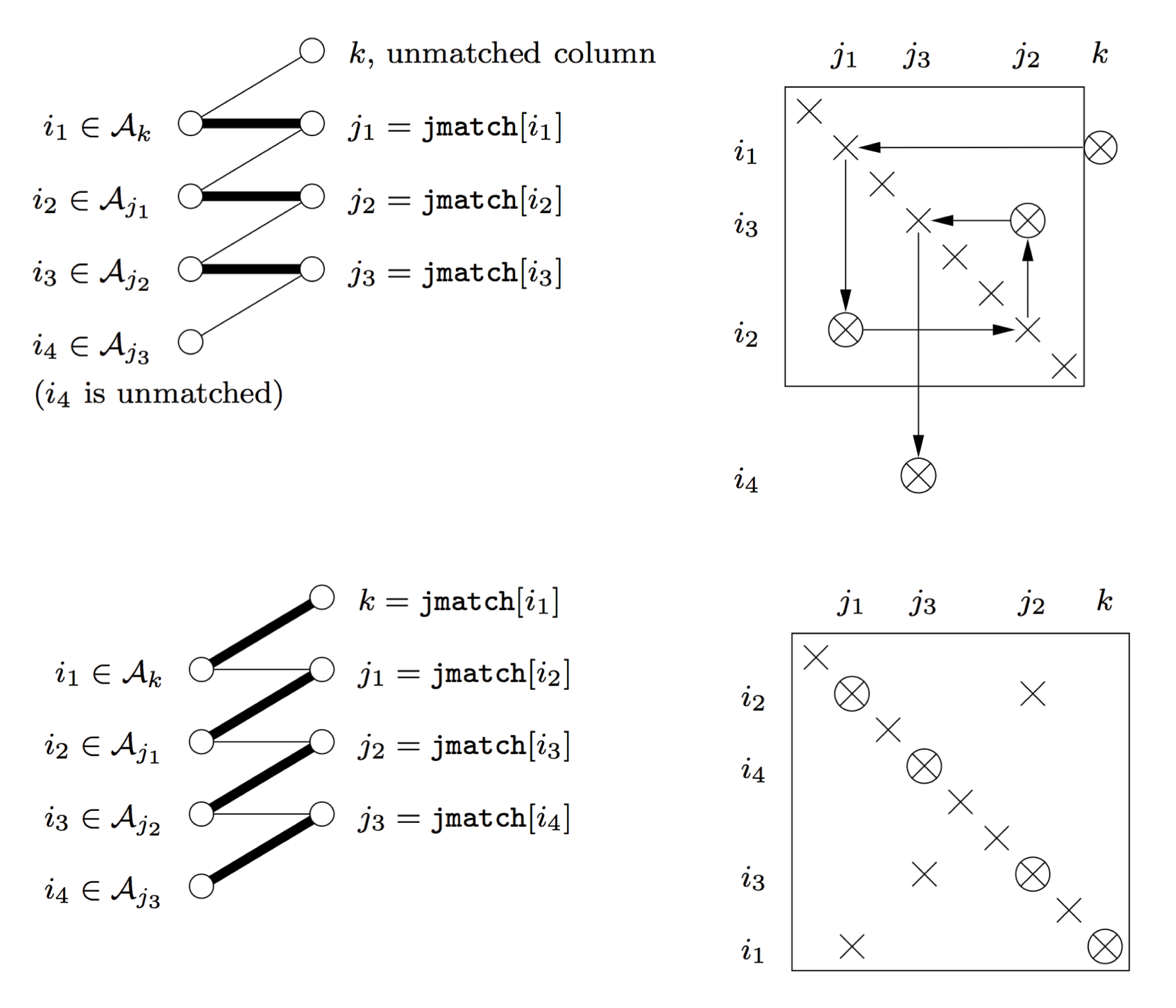
The augmenting path algorithms find the  ${\mathcal{M}}$-augmenting paths using a depth-first search (DFS) or a breadth-first search (BFS) in phases. Some versions use a hybrid of BFS and DFS. A simple DFS-based algorithm does one DFS for each unmatched column (or row) vertices. At each column
 $k$ the search path is extended with a row
 $r\in {\mathcal{A}}_{j}$ that is not visited (in the current DFS). Similarly, at each row
 $r$ the search path is extended with a column matched to
 $r$. If no such column exists then
 $r$ is unmatched, resulting in an alternating augmenting path. It is easy to see that the DFS-based algorithm does a lot more work than necessary. The algorithm can be implemented in
 $O(|A|n)$ work. The more common implementation of the algorithm uses a one-step BFS at each step of the DFS to short-circuit some work (Duff Reference Duff1981c). The technique is called lookahead. This technique has become the standard in DFS-based matching algorithms (Duff Reference Duff1981a, Davis Reference Davis2006). The lookahead method improves the runtime significantly even when the asymptotic complexity remains at
 $O(|A|n)$.
One DFS-based variation of the method uses multiple depth-first searches in a phase by finding multiple vertex-disjoint augmenting paths in each phase (Pothen and Fan Reference Pothen and Fan1990). This limits the vertices visited in each DFS, but it also requires us to use only the unmatched columns in each phase. This does not change the overall complexity but it improves the execution time even further. A recent variation of this algorithm, which visits the adjacency lists in alternating order in different depth-first searches within the same phase, improves the robustness of the algorithm to variation in the input order (Duff, Kaya and Uçar Reference Duff, Kaya and Uçar2011). BFS-based implementations of these algorithms are also possible.
Hopcroft and Karp (Reference Hopcroft and Karp1973) also use the idea of phases. Their algorithm uses a BFS at each phase from all the unmatched columns to find a set of shortest-length augmenting paths. A DFS algorithm is used to find maximal disjoint sets of augmenting paths from the original set. The next phase continues with all the unmatched columns (Hopcroft and Karp Reference Hopcroft and Karp1973). The theoretical complexity of the algorithm is  $O(|A|\sqrt{n})$. Duff and Wiberg (Reference Duff and Wiberg1988) have proposed a modification to this algorithm to find the shortest-length augmenting paths first but continue finding more augmenting paths from any unmatched rows left at the end of the phase in the original algorithm. They allow the last DFS to use all the edges in
 $G$. This change typically results in improved execution time. Recent comparisons of all these methods in serial show that the modified version of the DFS with multiple phases, and the Hopcroft–Karp algorithm with additional searches perform the best (Duff et al. Reference Duff, Kaya and Uçar2011). Multithreaded parallel versions of these algorithms have also been introduced recently (Azad et al. Reference Azad, Halappanavar, Rajamanickam, Boman, Khan and Pothen2012).
8.7.3 Block triangular form
The block triangular form reordering of a matrix is based on the canonical decomposition called the Dulmage–Mendelsohn decomposition using maximum matching on bipartite graphs (Dulmage and Mendelsohn Reference Dulmage and Mendelsohn1963). It is a useful tool for many sparse matrix algorithms and theorems. It is a permutation of a matrix  $A$ that reduces the work required for LU and QR factorization and provides a precise characterization of structurally rank deficient matrices.
We state some of the definitions common in the area (Pothen and Fan Reference Pothen and Fan1990). Let  ${\mathcal{M}}$ be a maximum matching in the bipartite graph
 $G(A)$. We can define the sets as follows:
∙
$R$, the set of all row vertices,∙
$C$, the set of all column vertices,∙
$VR$, the row vertices reachable by some alternating path from some unmatched row,∙
$HR$, the row vertices reachable by some alternating path from some unmatched column,∙
$SR=R\setminus (VR\cup HR)$,∙
$VC$, the column vertices reachable by some alternating path from some unmatched row,∙
$HC$, the column vertices reachable by some alternating path from some unmatched column, and∙
$SC=C\setminus (VC\cup HC)$.






The matrices  $A_{h}$,
 $A_{s}$, and
 $A_{v}$ are defined by the block diagonals formed by
 $HR\times HC$,
 $SR\times SC$ and
 $VR\times VC$ respectively. The coarse decomposition of the block triangular form is given by
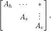 $$\begin{eqnarray}\left[\begin{array}{@{}ccc@{}}A_{h} & \cdots \, & \ast \\ & A_{s} & \vdots \\ & & A_{v}\end{array}\right]\!,\end{eqnarray}$$
The matrices  $A_{h}$,
 $A_{s}$, and
 $A_{v}$ can be further decomposed into block diagonal form.
 $A_{s}$ has the block triangular structure (called the fine decomposition)
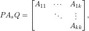 $$\begin{eqnarray}PA_{s}Q=\left[\begin{array}{@{}ccc@{}}A_{11} & \cdots \, & A_{1k}\\ & \ddots & \vdots \\ & & A_{kk}\end{array}\right]\!,\end{eqnarray}$$
where each diagonal block is square with a zero-free diagonal and has the strong-Hall property. It is this fine decomposition that is of most interest in the past work. The strong-Hall property implies full structural rank. The block triangular form (8.11) is unique, ignoring some trivial permutations (Duff Reference Duff1977a). There is often a choice of ordering within the blocks (the diagonal must remain zero-free). To solve  $Ax=b$ with LU factorization, only the diagonal blocks need to be factorized, followed by a block backsolve for the off-diagonal blocks. No fill-in occurs in the off-diagonal blocks. Sparse factorizations with the block triangular form have been in use for some time (Tewarson Reference Tewarson1972, Rose and Bunch Reference Rose, Bunch, Rose and Willoughby1972). Rose and Bunch (Reference Rose, Bunch, Rose and Willoughby1972) call this method partitioning the matrix, and consider factorizations using the partitioning.
Permuting a square matrix with a zero-free diagonal into block triangular form is identical to finding the strongly connected components of a directed graph,  $G(A)$. The directed graph is defined as
 $G(A)=(V,E)$ where
 $V=\{1,\ldots ,n\}$ and
 $E=\{(i,j)\,|\,a_{ij}\neq 0\}$. That is, the non-zero pattern of
 $A$ is the adjacency matrix of the directed graph
 $G(A)$. A strongly connected component is a maximal set of nodes such that for any pair of nodes
 $i$ and
 $j$ in the component, the paths
 $i{\rightsquigarrow}j$ and
 $j{\rightsquigarrow}i$ both exist in the graph.
The strongly connected components of a graph can be found in many ways. The simplest method uses two depth-first traversals, one of  $G(A)$, the second of the graph
 $G(A^{T})$ (Tarjan Reference Tarjan1972). However, depth-first traversals are difficult to parallelize. Slota, Rajamanickam and Madduri (Reference Slota, Rajamanickam and Madduri2014) rely on an approach that uses multiple steps, each of which can be parallelized effectively, to find the strongly connected components. They find trivial strongly connected components of size one or two first and then use breadth-first search to find the largest strongly connected component and an iterative colour propagation approach to find multiple small strongly connected components. This algorithm can be parallelized effectively in shared-memory (multicore) computers (Slota, Rajamanickam and Madduri Reference Slota, Rajamanickam and Madduri2014). An extension to manycore (GPUs and the Xeon Phi) accelerators requires modifications to algorithms that parallelize over edges instead of vertices (Slota, Rajamanickam and Madduri Reference Slota, Rajamanickam and Madduri2015). Finding the block triangular form using Tarjan’s algorithm has been the standard for some time (Gustavson Reference Gustavson, Bunch and Rose1976, Duff and Reid Reference Duff and Reid1978a, Duff and Reid Reference Duff and Reid1978b, Davis Reference Davis2006). More recently Duff and Uçar (Reference Duff and Uçar2010) showed that it is possible to recover symmetry around the anti-diagonal for the block triangular form of symmetric matrices.
8.8 Independent sets and elimination tree modification
The focus of this section is on pre-orderings for parallel factorizations. See also Section 6.4, where parallel algorithms for finding independent sets during numerical factorization are discussed.
The methods discussed here fall into different categories based on the dependency graph they use and the factors used to arrive at the parallel orderings. All the methods use an implicit or explicit directed acyclic graph which represent the set of operations, pivot sequence or block ordering to improve the parallel efficiency or completion time along with the considerations for fill.
On circuit matrices, early bandwidth-reducing orderings, block triangular forms or envelope-based methods were less useful, as the matrices are highly irregular. Fine-grained task graphs were considered, where each floating-point operation and its dependency is considered in the task graph along with a local heuristic to reduce the floating-point operation and the length of the critical path in the task graph (Huang and Wing Reference Huang and Wing1979, Wing and Huang Reference Wing and Huang1980). A level scheduling ordering was used to find the critical path. The approach of Huang and Wing (Reference Huang and Wing1979) is one of the earliest efforts to include the ordering quality as part of the metric. Earlier heuristics considered just finding the independent sets (Calahan Reference Calahan1973). Smart and White (Reference Smart and White1988) use the Markowitz counts to find candidate pivots and find the independent sets within those candidates to reduce the critical path length.
These scheduling strategies are harder for the sparse problems than dense factorizations, as the optimal ordering depends on both the structure of the problem and the fill (Srinivas Reference Srinivas1983). Later algorithms rely on an elimination tree for scheduling the pivots rather than the operations (Jess and Kees Reference Jess and Kees1982). Jess and Kees use a fill-reducing ordering first and then consider pivots that are independent to be factorized in parallel. There is also another level of parallelism in factoring a pivot itself, which some of these papers consider. Combining the method of Jess and Kees (Reference Jess and Kees1982) with minimum degree ordering has been explored as well (Padmini, Madan and Jain Reference Padmini, Madan and Jain1998). Padmini et al. avoid using the chordal graph of the filled matrix, and use the graph of  $A$ to arrive at the orderings.
In contrast to Jess and Kees (Reference Jess and Kees1982), there are other approaches that consider finding the independent sets given a specific pivot sequence (Peters Reference Peters1984, Reference Peters and Evans1985). There exist two different implementations of the second stage of the Jess and Kees method (to find the independent sets) (Lewis, Peyton and Pothen Reference Lewis, Peyton and Pothen1989, Liu and Mirzaian Reference Liu and Mirzaian1989). The implementation of Liu and Mirzaian is more expensive than the fill-reducing orderings, as observed by Lewis et al. (Reference Lewis, Peyton and Pothen1989). They propose using a clique tree representation of the chordal graph of the factors, G( $L+L^{T}$), to find the maximum independent sets, making this step cheaper than the fill-reducing orderings. The primary cost of Liu and Mirzaian’s method is in maintaining degrees of the nodes, as other nodes get picked in different independent sets. The clique tree representation simplifies this cost.
There are other approaches, such as the tree rotations introduced by Liu to reduce the height of the elimination trees (Liu Reference Liu1988a). Tree rotations can be used for improving the parallelism (Liu Reference Liu1989d), and work better than the Liu and Mirzaian method. Duff and Johnsson (Reference Duff, Johnsson and Carey1989) compare minimum degree, nested dissection and minimum height orderings. They introduce the terminology for inner (single pivot level) and outer (multiple pivots) parallelism. They also show that nested dissection performs well in exposing parallelism. The superiority of nested dissection to other fill-reducing ordering methods to expose parallelism was studied by Leuze (Reference Leuze1989), who also introduces a greedy heuristic and an algorithm based on vertex covers to find the independent sets, the latter of which is better than nested dissection.
Davis and Yew (Reference Davis and Yew1990) show that for unsymmetric problems one could do a non-deterministic parallel pivot search to find groups of compatible pivots for a rank- $k$ update, instead of relying on an etree-based approach that symmetrizes the problems. The pivot sets are found in parallel, where conflicts are avoided using critical sections. A somewhat different approach is to use a fill-reducing ordering first and then use a fill-preserving reordering to improve parallelism (Kumar, Eswar, Sadayappan and Huang Reference Kumar, Eswar, Sadayappan and Huang1994, Kumar et al. Reference Kumar, Eswar, Sadayappan and Huang1994). Once the reordering is done, this method maps the pivots to the processors as well (Kumar et al. Reference Kumar, Eswar, Sadayappan and Huang1994). While the height of the elimination tree serves well for exposing the parallelism, it assumes a unit cost for the node elimination and does not model the communication costs. It is possible to model the communication costs and order the pivots based on the communication costs (Lin and Chen Reference Lin and Chen1999) or based on a completion cost metric (Lin and Chen Reference Lin and Chen2005) as well. These extensions allow the reordering algorithm to use more information, and hence obtain better reorderings.
9 Supernodal methods
All of the numerical factorization algorithms discussed so far depend on gather/scatter operations for all of their operations, on individual sparse row or column vectors. The sparse matrix data structures, as well, represent individual rows or columns one at a time, as independent entities. However, a matrix factorization (LU, Cholesky, or QR) often has columns and rows with duplicate structure. The supernodal method exploits this to save time and space. It saves space by storing less integer information, and it saves time by operating on dense submatrices rather than on individual rows and columns. Dense matrix operations on the dense submatrices of the supernodes exploit the memory hierarchy far better than the irregular gather/scatter operations used in all the factorization methods discussed so far in this survey. The frontal and multifrontal methods also exploit these structural features of the factorization, using a very different strategy (Sections 10 and 11).
Section 9.1 below considers the supernodal method for the symmetric case: Cholesky and  $\text{LDL}^{\text{T}}$ factorization. The symmetric method precedes the development of the supernodal LU factorization method discussed in Section 9.2.
9.1 Supernodal Cholesky factorization
The supernodal Cholesky factorization method exploits the fact that many columns of the sparse Cholesky factor  $L$ have identical non-zero pattern, or nearly so.
Consider equation (4.3), which states that the non-zero pattern  ${\mathcal{L}}_{j}$ of a column
 $j$ is the union of its children, plus the entries in the
 $j$th column of
 $A$. A node often has only a single child
 $c$ in the elimination tree, and the
 $j$th column of
 $A$ may add no additional entries to the pattern. The
 $j$th column of
 $A$ would of course contribute to the numerical value of the
 $j$th column of
 $L$, but at this point it is only the non-zero structure that is of interest, not the values. If the matrix is permuted according to the elimination tree postordering, this single child of
 $j$ will be column
 $j-1$. This case can repeat, resulting in a chain of
 $c>1$ nodes in the elimination tree. Grouping these
 $c$ columns of
 $L$ together results in a single fundamental supernode (Liu, Ng and Peyton Reference Liu, Ng and Peyton1993). During numerical factorization, a supernode with
 $c$ columns of
 $L$ is represented as a dense lower trapezoidal submatrix of size
 $r\times c$, where
 $r$ is the number of non-zeros in the first, or leading, column of the supernode. The same nodes can be folded together in the elimination tree, and represented with a single node per supernode, resulting in the supernodal elimination tree.
The left-looking supernodal Cholesky factorization is illustrated in the MATLAB script chol_super below. Compare it with chol_left in Section 5.3. The algorithm starts with a fill-reducing ordering (Section 8), and then finds the elimination tree and its postordering. The tree is stored as the parent array, where parent(j) is the parent of node j. The postordering is combined with the fill-reducing ordering, which places parents and children close to one another, and thus increases the sizes of the fundamental supernodes. The amount of fill-in and work is not affected by the postordering (Liu Reference Liu1990), since the resulting graphs are isomorphic. Next, the MATLAB script finds column counts and the postordered tree (via symbfact). It recomputes the tree to keep the script simple, but it can be found from the original tree computed by the etree function.
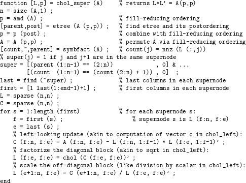
The term super(j) is true if column j and j+1 fit into the same supernode, which happens when the parent of j is j+1 and the two columns share the same non-zero pattern. This is not quite the same as a fundamental supernode, since the latter would require j to be the only child of j+1, but it makes for a very simple MATLAB one-liner to find all the supernodes. To improve performance, supernodes are often extended in size beyond this test, to put j and j+1 together if their patterns are very similar, not necessarily equal. These are called relaxed supernodes. Note that the test for similar non-zero patterns does not need the patterns themselves, but just the column counts, since the pattern of a child is always a subset of the pattern of its parent. This chol_super script does not exploit relaxed supernodes.
The numeric factorization computes one supernodal column of  $L$ at a time. It first computes the update term C, one per descendant supernode. For simplicity, this is shown as single matrix–matrix multiply in the script. In practice, this is always done for each descendant supernodal column, just as the left-looking non-supernodal method (chol_left) traverses across each descendant column (the for j=find(L(k,:)) traversal of the
 $k$th row subtree).
A supernodal update is shown in Figure 9.1. The descendant  $d$ corresponds to three adjacent columns of
 $L$,
 $d_{f}$ to
 $d_{e}$. Its non-zero pattern is a subset of the target supernode
 $s$, consisting of four columns
 $s_{f}$ to
 $s_{e}$. In each supernode, all entries in any given row are either all zero or all non-zero. The computation of C for this supernode requires a 6
 $\times$ 3 times 3
 $\times$ 3 dense matrix multiply, giving a dense 6
 $\times$ 3 update that is subtracted from a 6
 $\times$ 3 submatrix (shown in dark circles) of the 9
 $\times$ 4 target supernode
 $s$.
Left-looking update in a supernodal Cholesky factorization. Solid circles denote entries that take part in the supernodal update of the target supernode  $s$ with descendant supernode
 $d$. Grey circles are non-zero but do not take part in the update of
 $s$ by its descendant
 $d$.
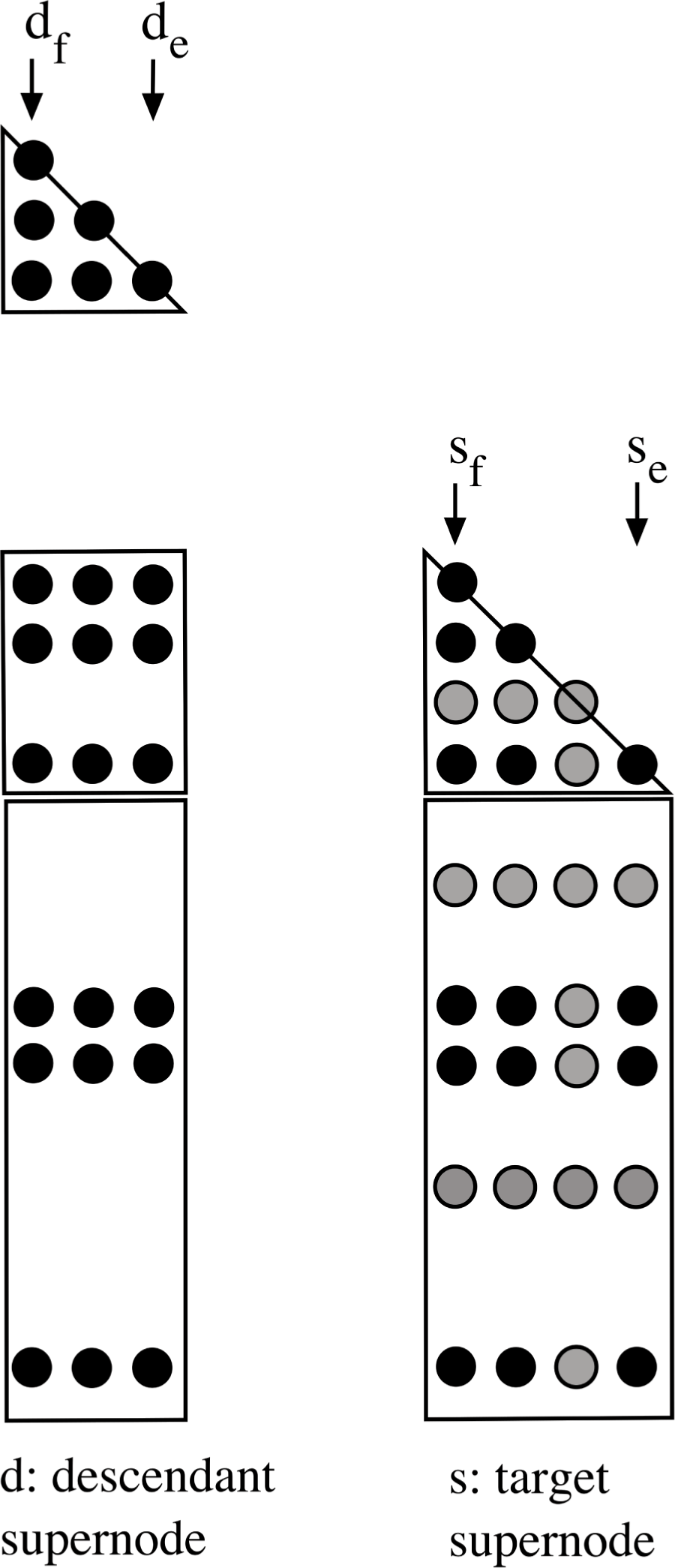
9.1.1 Sequential supernodal Cholesky factorization
Supernodes in their current form are predated by several related developments. George (Reference George1977a) considered a partitioning for finite element matrices in which each block column had a dense triangular part, just like supernodes. Unlike supernodes, the rows below the triangular part were represented in an envelope form, which (in current terminology) corresponds to a single path in the corresponding row subtrees.
George and McIntyre (Reference George and Mcintyre1978) used a supernodal structure for the symbolic pattern of  $L$ for a minimum degree ordering method for finite element problems. George and Liu (Reference George and Liu1980b) then extended this idea for a general minimum degree ordering method, in which groups of nodes (columns) with identical structure are merged (referred to as indistinguishable nodes). George and Liu (Reference George and Liu1980c) exploited the supernodal structure of
 $L$ in their compressed-index scheme for symbolic factorization, which represents the pattern of
 $L$ with less than one integer per non-zero on
 $L$. These compact representations (discussed in Section 8) are a precursor to the supernodal method, which extends this idea into the numeric factorization.
The first supernodal numeric factorization was a left-looking method by Ashcraft et al. (Reference Ashcraft, Grimes, Lewis, Peyton and Simon1987), based on the observations in the symbolic methods just discussed. Pothen and Sun (Reference Pothen, Sun, Coleman and Li1990) generalize the supernodal elimination tree (as the clique tree) and also extend the symbolic skeleton matrix  $\widehat{A}$ used in the row/column count algorithm (Section 4.2) to the supernodal skeleton matrix.
Rothberg and Gupta (Reference Rothberg and Gupta1991, Reference Rothberg and Gupta1993) show that the supernodal method can also be implemented in a right-looking fashion. With a right-looking approach, the supernodal method becomes more similar to the multifrontal method (Section 11), which is also right-looking, and which also exploits dense submatrices. The supernodes, in fact, correspond exactly to the fully assembled columns of a frontal matrix in the multifrontal method. The difference is that the right-looking supernodal method applies its updates directly to the target supernodes (to the right), and thus it does not require the stack of contribution blocks used by the multifrontal method to hold its pending updates. The supernodal update shown in Figure 9.1 is the same, except that as soon as the supernode  $d$ is computed, its updates are applied to all supernodes to the right that require them. The target supernodes correspond to a subset of the ancestors of
 $d$ in the supernodal elimination tree.
Ng and Peyton (Reference Ng and Peyton1993a) compare the performance of the left-looking (non-supernodal) method, two variants of the left-looking supernodal method, and two variants of the multifrontal method. In one supernodal method, the key kernel is the update of a single target column with a descendant supernode. The second obtains higher performance by relying on a kernel that updates all the columns in a target supernodal column with a descendant supernode. This reduces memory traffic. They also consider two methods for determining the set of descendant supernodes that need to update the target supernode: a link list, and a traversal of the  $k$th row subtree.
The supernodal method requires an extension of the symbolic analysis for the column-wise Cholesky factorization. Liu et al. (Reference Liu, Ng and Peyton1993) show how to find supernodes efficiently, without having to build the entire pattern of  $L$ first, column-by-column. The resulting algorithm takes nearly
 $O(|A|)$ time, and allows the subsequent supernodal symbolic factorization to know ahead of time what the supernodes are.
Both the supernodal method and the multifrontal method obtain high performance due to their reliance on dense matrix operations on dense submatrices (the BLAS). These dense kernels are highly efficient because of their re-use of cache. Rozin and Toledo (Reference Rozin and Toledo2005) compare the cache re-use of both the supernodal and multifrontal methods, and show that some classes of matrices are better suited to each method.
For very sparse matrices, the simpler up-looking or left-looking (non-supernodal) methods can be faster than the supernodal method. If the dense submatrices are too small, it makes little sense to try to exploit them. MATLAB relies on CHOLMOD for chol and  (Chen et al. Reference Chen, Davis, Hager and Rajamanickam2008), which includes both the left-looking supernodal method (with supernode–supernode updates), and the up-looking method (Section 5.2). CHOLMOD finds the computational intensity as a by-product of the symbolic analysis (the ratio of flop count over
 $|L|$). If this is high (over 40), then it uses a left-looking supernodal method. Otherwise, it uses the up-looking method, which is faster in this case. Its supernodal symbolic analysis phase determines the relaxed supernodes based solely on the elimination tree and the row/column counts of
 ${\mathcal{L}}$, an extension of Liu et al.’s (Reference Liu, Ng and Peyton1993) method for fundamental supernodes.
9.1.2 Parallel supernodal Cholesky factorization
The supernodal method is well-suited to implementations on both a shared-memory and distributed-memory parallel computers.
Ng and Peyton (Reference Ng and Peyton1993b) consider the first parallel supernodal Cholesky factorization method, and its implementation on a shared-memory computer. It uses a set of lists for pending supernodal updates, much like how the method of George et al. (Reference George, Heath, Liu and Ng1986a) uses them for a parallel column-wise algorithm.
The symbolic factorization phase is very hard to parallelize, since it requires time that is essentially proportional to the size of its output, a compact representation of the supernodal symbolic pattern,  ${\mathcal{L}}$. However, it is very useful on a distributed-memory computer, where all of
 ${\mathcal{L}}$ never resides in the memory of a single processor. Ng (Reference Ng1993) considers this case, extending the work of George et al. (Reference George, Heath, Ng and Liu1987, Reference George, Heath, Liu and Ng1989a) to the supernodal realm.
Eswar, Sadayappan, Huang and Visvanathan (Reference Eswar, Sadayappan, Huang and Visvanathan1993b) present two distributed-memory supernodal methods (both left- and right-looking), using a one-dimensional distribution of supernodal columns. Large supernodes are split and distributed, as well. Comparing these two methods, they find that the left-looking method is faster because of the reduction in communication volume. Communication volume in the right-looking method is reduced by aggregating the updates, depending upon how much local memory is available to construct the aggregate updates (Eswar et al. Reference Eswar, Huang and Sadayappan1994).
Rothberg and Gupta (Reference Rothberg and Gupta1994) extend their right-looking supernodal approach, which differs from the left-looking method in one very important respect. The left-looking method described so far uses a one-dimensional distribution of columns (or supernodes) to processors. Rothberg and Gupta present a two-dimensional distribution that improves parallelism and enhances scalability. Both rows and columns are split according to the supernodal partition, and each supernode is spread across many processors. For example, in Figure 9.1, the block consisting of rows  $s_{f}$ to
 $s_{e}$, and columns
 $d_{f}$ to
 $d_{e}$ would reside on a single processor. Rothberg (Reference Rothberg1996) compares the performance of both one- and two-dimensional methods, and the multifrontal method, on distributed-memory computers. Parallel sparse Cholesky factorization places a higher demand on the communication system of a distributed-memory computer since it has a lower computation-to-communication ratio as compared with dense factorization. The method uses a cyclic two-dimensional distribution of blocks; Rothberg and Schreiber (Reference Rothberg and Schreiber1994) describe a more balanced distribution for this method.
Rauber, Rünger and Scholtes (Reference Rauber, Rünger and Scholtes1999) consider shared-memory parallel implementations of both left-looking and right-looking (non-supernodal) Cholesky and two variants of right-looking supernodal Cholesky factorization. The variants rely on different task scheduling and synchronization methods, with dynamic assignments of tasks to processors. Each variant uses a one-dimensional distribution of columns (or supernodal columns) to processors.
Hénon, Ramet and Roman (Reference Hénon, Ramet and Roman2002) combine both left- and right-looking approaches in their parallel distributed-memory supernodal factorization method, in PaStiX. They use a one-dimensional distribution for small supernodes, and a two-dimensional distribution for large ones. The latter occur towards the root of the elimination tree. Updates are aggregated if sufficient memory is available, and only partially aggregated otherwise.
Lee, Kim, Hong and Lee (Reference Lee, Kim, Hong and Lee2003) extend the method of Rothberg and Gupta (Reference Rothberg and Gupta1994) in their distributed-memory sparse Cholesky factorization. It uses the same right-looking method with a two-dimensional distribution of the supernodes. They introduce a task scheduling method based on a directed acyclic graph (DAG), rather than the elimination tree. They compare four methods: (1) non-supernodal, with a one-dimensional distribution (George et al. Reference George, Heath, Liu and Ng1988a), (2) supernodal, with cyclic two-dimensional distribution (Rothberg and Gupta Reference Rothberg and Gupta1994), (3) supernodal, with more balanced two-dimensional distribution (Rothberg and Schreiber Reference Rothberg and Schreiber1994), and (4) their DAG-based method. Task scheduling based on DAGs has also been used for the multifrontal method (Section 11).
Rotkin and Toledo (Reference Rotkin and Toledo2004) combine a left-looking supernodal Cholesky factorization with a right-looking (non-multifrontal) strategy in their out-of-core method. Their hybrid method is closely related to Rothberg and Schreiber’s (Reference Rothberg and Schreiber1999) out-of-core method, which combines a left-looking supernodal method with a right-looking multifrontal method (their method is discussed in Section 11). In Rotkin and Toledo’s method, submatrices corresponding to subtrees of the elimination tree are factorized in a supernodal left-looking manner. Some descendants may reside on disk, and these are brought back in as needed. Once a supernode is computed, it updates its ancestors in the current subtree, which is in main memory, using a right-looking supernodal strategy. Meshar, Irony and Toledo (Reference Meshar, Irony and Toledo2006) extend this method to the symmetric indefinite case, in which numerical pivoting must be considered.
Time and memory are not the only resource an algorithm requires. Power consumption is another resource that algorithm developers rarely consider. Chen, Malkowski, Kandemir and Raghavan (Reference Chen, Malkowski, Kandemir and Raghavan2005) present a parallel supernodal Cholesky factorization that addresses this issue via voltage and frequency scaling. A CPU running at a lower voltage/frequency is slower but uses much less power. In their method, CPUs that perform computations for supernodes on the critical path run at full speed, whereas CPUs computing tasks not on the critical path have their voltage/frequency cut back. Slowing down these CPUs does not increase the overall runtime, but power consumption is reduced.
Hogg, Reid and Scott (Reference Hogg, Reid and Scott2010) presents a DAG-based scheduler for a parallel shared-memory supernodal Cholesky method, HSL_MA87. They also give a detailed description of many other methods and an extensive performance comparison with those methods.
Lacoste et al. (Reference Lacoste, Ramet, Faverge, Ichitaro and Dongarra2012) describe a DAG-based scheduler for PaStiX, and also present a GPU-accelerated supernodal Cholesky factorization. The GPU aspects of PaStiX are discussed in Section 12.3.
9.2 Supernodal LU factorization
The supernodal strategy also applies to LU factorization of unsymmetric and rectangular matrices. Demmel et al. (Reference Demmel, Eisenstat, Gilbert, Li and Liu1999a) introduced the idea of unsymmetric supernodes, and implemented them in their left-looking method, SuperLU. Its derivation is analogous to the left-looking LU factorization. Consider equation (6.2). In the supernodal left-looking LU factorization, the  $(2,2)$-block of
 $A$,
 $L$, and
 $U$ becomes a matrix (one supernode) instead of a scalar.
In a symmetric factorization, the factors  $L$ and
 $L^{T}$ have the same non-zero pattern, so it suffices to define the supernodes based solely on the pattern of
 $L$. In an unsymmetric factorization (
 $A=LU$),
 $L$ can differ from
 $U^{T}$. Thus, Demmel et al. (Reference Demmel, Eisenstat, Gilbert, Li and Liu1999a) consider many possible types of unsymmetric supernodes, but rely on only one of them in their method: an unsymmetric supernode is a contiguous set of columns of
 $L$ (say
 $f$ to
 $e$), all of which have the same non-zero pattern, and they include in this supernode the same columns of
 $U$. The diagonal block of a supernode in
 $L$ is thus a dense lower triangular matrix. This definition is the same as a supernode in a Cholesky factor, for
 $L$. They show that the non-zero pattern of rows
 $f$ to
 $e$ of
 $U$ has a special structure; those rows of
 $U$ can be represented as a dense envelope, with no extra entries. That is, if
 $u_{ik}\neq 0$ for some
 $i\in \{f,\ldots ,e\}$, then all
 $u_{tk}\neq 0$ for all
 $t\in \{i+1,\ldots ,e\}$. This structure of
 $U$ is very similar to George’s (Reference George1977a) partitioning of the Cholesky
 $L$ for finite element matrices, which predates supernodal methods. Just as in supernodal Cholesky factorization, the method relies on relaxed supernodes where the pattern of the columns of
 $L$ need not be identical, to reduce memory usage and improve performance.
An unsymmetric supernode is shown in Figure 9.2. The lower triangular part of supernode  $s$ is the same as Figure 9.1, but the pattern of
 $U$ differs. The descendant
 $d$ has a structure of
 $L(s_{f}:s_{e},d_{f}:d_{e})$ that is the same as the symmetric supernode, but the transposed part in
 $U$, namely,
 $U(d_{f}:d_{e},s_{f}:s_{e})$ differs. This part of
 $U$ is in envelope form. The update of
 $d$ to
 $s$ must also operate on the columns in
 $U$ of the target supernode
 $s$ (namely, rows
 $d_{e}+1$ to
 $s_{e}$), and thus a few entries are added there for this figure.
Left-looking update in a supernodal LU factorization. Solid entries take part in the update of  $s$ by supernode
 $d$. Grey entries are non-zero but are not modified by this update.
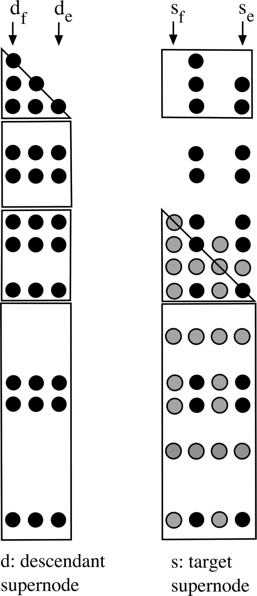
This definition of an unsymmetric supernode does not permit the exploitation of simple dense matrix–matrix multiplication kernels (GEMM) in the supernodal update. However, since the blocks of  $U$ have a special structure (a dense envelope), good performance can still be obtained using a sequence of dense matrix–vector multiplies (GEMV), where the structure of each is very similar, and the matrix (from the descendant supernode
 $d$) is re-used for each operation. SuperLU is partly right-looking, as it can update more than one target supernode
 $s$ with a single updating node
 $d$. Up to
 $w$ individual columns are updated at a time, where
 $w$ is selected based on the cache size.
Demmel et al. (Reference Demmel, Eisenstat, Gilbert, Li and Liu1999a) extend the symbolic LU analysis discussed in Section 6.1, and determine an upper bound on the patterns  $L$ and
 $U$, by accounting for worst-case partial pivoting with row interchanges in the numeric factorization.
Like its Cholesky variant, the supernodal LU factorization method is amenable to a parallel implementation. Fu, Jiao and Yang (Reference Fu, Jiao and Yang1998) present a parallel right-looking method called S* for a distributed-memory computer. They employ a two-dimensional supernode partition, analogous to the two-dimensional supernode partitioning of Rothberg and Gupta (Reference Rothberg and Gupta1994) and Rothberg and Schreiber (Reference Rothberg and Schreiber1994) for sparse Cholesky factorization. The matrix  $L+U$ is partitioned symmetrically, in the sense that both rows and columns are partitioned identically. This gives square blocks on the diagonal of
 $L+U$, and rectangular off-diagonal blocks. In Figure 9.2,
 $L(s_{f}:s_{e},d_{f}:d_{e})$ would form a single 4
 $\times$ 3 block, for example. The method is further developed by Shen, Yang and Jiao (Reference Shen, Yang and Jiao2000), as the algorithm S+. The method uses a different column elimination tree, further analysed by Oliveira (Reference Oliveira2001), called the row-merge tree. The trees are very similar. In the row-merge tree,
 $k$ is the parent of
 $j$ if
 $u_{jk}\neq 0$ is the first off-diagonal entry in row
 $j$, except that
 $j$ is a root if there is only one non-zero in the
 $j$th column of
 $L$. Their parallel task scheduling and data mapping allocates the two-dimensional blocks of the matrix onto a two-dimensional processor grid, and relies on the row-merge tree to determine which supernodal updates can occur simultaneously.
Demmel, Gilbert and Li (Reference Demmel, Gilbert and Li1999b) present a shared-memory version of SuperLU, called SuperLU_MT. It is a left-looking method that exploits two levels of parallelism. First, supernodes in independent subtrees in the column elimination tree can be done in parallel. Second, supernodes with an ancestor/descendant relationship can be pipelined, where an ancestor can apply updates from other descendant supernodes which have already been completed.
Schenk, Gärtner, Fichtner and Stricker (Reference Schenk, Gärtner and Fichtner2000, Reference Schenk, Gärtner, Fichtner and Stricker2001) combine left- and right-looking updates in PARDISO, a parallel method for shared-memory computers. It assumes a symmetric non-zero pattern of  $A$, which allows for use of the Level 3 BLAS (dense matrix–matrix multiply). In contrast to SuperLU (which allows for arbitrary numerical pivoting), PARDISO performs numerical pivoting only within the diagonal blocks of each supernode (static pivoting). Schenk and Gärtner (Reference Schenk and Gärtner2002) improve scalability of PARDISO with a more dynamic scheduling method. They modify the pivoting strategy by performing complete pivoting within each supernode, and include a weighted matching and scaling method as a preprocessing step, which reduces the need for numerical pivoting (Schenk and Gärtner Reference Schenk and Gärtner2004).
Li and Demmel (Reference Li and Demmel2003) extend SuperLU to the distributed-memory domain with SuperLU_DIST, a right-looking method. This method differs in one important respect from SuperLU. Like PARDISO, it only allows for static numerical pivoting. Amestoy, Duff, L’Excellent and Li (Reference Amestoy, Duff, L’Excellent and Li2001b) compare an early version of SuperLU_DIST with the distributed-memory version of MUMPS, a multifrontal method. MUMPS is generally faster and allows for more general pivoting and can thus obtain a more accurate result, at the cost of increased fill-in and higher memory requirements than SuperLU_DIST. One step of iterative refinement is usually sufficient for SuperLU_DIST to reach the same accuracy, however. Both methods have the same total communication volume but the multifrontal method requires fewer messages. In a subsequent paper (Amestoy, Duff, L’Excellent and Li Reference Amestoy, Duff, L’Excellent and Li2003a), they show how MPI implementations affect both solvers.
Li (Reference Li2005) provides an overview of all three SuperLU variants: (1) the left-looking sequential SuperLU, (2) the left-looking parallel shared-memory SuperLU_MT, and (3) the right-looking parallel distributed-memory SuperLU_DIST. The last method has the highest level of parallelism for very large matrices. In a subsequent paper, Li (Reference Li2008) considers the performance of these methods when each node of the computer consists of a tightly coupled multicore processor. Grigori and Li (Reference Grigori and Li2007) present an accurate simulation-based performance model for SuperLU_DIST, which includes the speed of the processors, memory systems, and the latency and bandwidth of the interconnect.
10 Frontal methods
The frontal method was introduced by B. M. Irons (Reference Irons1970). It was first described in the literature in 1970, although its use in the industry predates this. It originates in the solution of symmetric positive definite banded linear systems arising from the finite element method, but it has been adapted to the unsymmetric case by Hood (Reference Hood1976) and to the symmetric indefinite case by Reid (Reference Reid and Duff1981). It is based on Gaussian elimination and is presented as an alternative and improvement to Gaussian band algorithms.
In the finite element formulation, the stiffness matrix  $A$ is expressed as the sum of finite element contributions
 $$\begin{eqnarray}A=\mathop{\sum }_{i}A^{(i)}.\end{eqnarray}$$
Each element is associated with a set of few variables and each variable is related to a small set of elements.
The frontal method relies on the fundamental observation that, given the linear nature of the Gaussian elimination process, a finite element may start to be eliminated before being fully assembled. Specifically, the variables to be eliminated need to be fully summed but the ones to be updated need not. Moreover, elements can be summed in any order, and the updates from eliminated variables can also be done in any order.
The frontal method follows some key steps. First, it defines and allocates a front: a dense square submatrix in which all operations take place. Its minimum storage requirement can be assessed directly from the ordering in which the elements are assembled, although its effective size depends on the amount of available core (memory). As the elimination proceeds, it advances diagonally down the stiffness matrix, one element at a time.
Second, the frontal method alternates between the assembly of finite elements and the elimination and update of variables. The finite elements are assembled, one after another, following a predefined ordering, until the front gets full. A partial factorization is then applied to the front: the fully summed variables are eliminated, one after another, and each elimination is followed by the update of the other non-eliminated variables in the front.
Third, since the eliminated variables will no longer be used during the factorization process, they are removed from the frontal matrix and stored elsewhere, usually on disk, leaving the free space for the next elements to be assembled. The frontal process continues until all elements have been assembled and all variables have been eliminated.
Finally, the solution of the system is obtained using standard forward and backward substitutions.
From an algebraic point of view, a front is a dense submatrix of the overall system. It can be written as
 $$\begin{eqnarray}\left(\begin{array}{@{}cc@{}}F_{11} & F_{12}\\ F_{12}^{T} & F_{22}\end{array}\right)\!,\end{eqnarray}$$
where  $F_{11}$ contains the fully summed rows and columns and is thus factorized. Multipliers are stored over
 $F_{12}$ and the Schur complement is formed as
 $F_{22}-F_{12}^{T}F_{11}^{-1}F_{12}$ and updates
 $F_{22}$.
From a geometric point of view, a front can be seen as a wave that traverses the finite element mesh during the elimination process. A variable becomes ‘active’ on its first appearance in the front and is eliminated immediately after its last appearance, that is, it has begun to be assembled but is not yet eliminated. The front is thus the set of active variables that separate the eliminated variables (behind the front) from the not-yet activated variables (after the front) in the finite element mesh.
10.1 Ordering of the finite elements
Ordering techniques (see Section 8) have an impact on the frontal method. In the frontal method, the order in which the elements (resp. variables) are assembled is critical in element (resp. non-element) problems. The ordering is chosen in such a way as to keep the size of the fronts as small as possible, similar to the logic of bandwidth minimization, in order to reduce the arithmetic operations and storage requirements. Reid (Reference Reid and Duff1981) cites the Cuthill and McKee (Reference Cuthill and Mckee1969), Cuthill (Reference Cuthill, Rose and Willoughby1972) and improvements by Gibbs, Poole and Stockmeyer (Reference Gibbs, Poole and Stockmeyer1976a) as the established reordering techniques for frontal methods. He also notices that the reverse Cuthill–McKee technique developed by George (Reference George1971) often yields worthwhile improvements, essentially because the variables associated with a single or pair of elements in the same level set become fully summed, and are thus eliminated soon after becoming active, so they do not contribute to an increase in the front size. Finally, he notices that the minimum degree ordering is remarkably successful in the case of sparse symmetric matrices. Indeed, this technique has been used successfully, and is still widely used as an ordering of choice in the frontal and multifrontal methods.
10.2 Extensions of the frontal method
Although the same storage area is allocated for all the fronts, the effective size of the successive fronts may vary during the elimination process, possibly introducing some sparsity in the front. Thompson and Shimazaki (Reference Thompson and Shimazaki1980) proposed the frontal-skyline method, a hybrid method that requires fewer transfers to/from disk than either the frontal or blocked-skyline methods, and that requires the same minimum core as the frontal method. It behaves identically to the frontal method but uses an efficient compact skyline storage scheme (column, envelope or profile), similar to the blocked-skyline method, which circumvents the vacancies that would appear in the front using the frontal method when the size of the front increases. The method therefore proves most valuable for problems which have front widths that vary greatly from one position in the mesh to another.
Moreover, in an in-core context, when using a direct method, it is important to know whether a given problem can be solved for a given core size. Amit and Hall (Reference Amit and Hall1981) proposed a lower bound on the minimal length of the front, independent of the ordering of the nodes, as the size of the causey of maximal length. They define a causey as a path in a graph that stretches from the boundaries and where the distance of each of its nodes to the boundary is minimal. They also describe an algorithm for finding a maximal causey. Their result is an extension of that of George (Reference George1973) to the wider class of simplicial triangulations graphs, and their estimate is not as sharp on the class of general graphs but is still a lower bound.
Melhem (Reference Melhem1988) suggests a window-oriented variation of the frontal technique combining features from band solvers. The computations are confined within a sliding window of  ${\it\sigma}$ contiguous rows of the stiffness matrix. These rows are assembled and factorized in sequential order, allowing for an automatic detection (without preprocessing) of the moment when rows become fully summed. These rows, which appear at the top of the window, are factorized and then removed from memory, allowing the window to move downward. The simplification of data management and bookkeeping comes at the price of larger memory requirement. Indeed, the optimal width of the delayed front,
 ${\it\sigma}_{\min }$, is usually larger than the maximum size of the active front, although Melhem proposes different bounds for the optimal value
 ${\it\sigma}_{\min }$ under different hypotheses, and proves that, for meshes encountered in practical applications,
 ${\it\sigma}_{\min }$ is smaller than the bandwidth of the stiffness matrix. Melhem also describes an algorithm allowing the interleaving of the assembly and factorization of the stiffness matrix and discusses two possible parallel approaches using the window-oriented assembly scheme.
Duff (Reference Duff1984a) proposes extensions of the frontal method to the general case of non-element problems and of unsymmetric matrices, together with their implementation in the MA32 package. In the case of non-element problems, the rows of the sparse matrix (rather than the usual finite elements) are assembled one after another in the frontal matrix. A variable is considered to be fully summed when all the equations it appears in are assembled. In the case of unsymmetric matrices, Duff also notes that the frontal matrix is rectangular.
10.3 Numerical stability
In the case where the matrix is not symmetric positive definite, numerical stability considerations have to be taken into account. Hood (Reference Hood1976) presents a variant of the frontal method for unsymmetric matrices. The factorization process is modified: before each elimination, the largest entry in the pivotal search space is determined and the corresponding pivotal row is then used to eliminate the coefficients in the pivotal column. As extending the search space to the entire stiffness matrix would require too much memory, Hood restricts the pivot search space to the submatrix of fully summed rows and columns in the front ( $F_{11}$ in equation (10.2)). Moreover, as a combination of the already reduced search space with another pivotal strategy would further reduce the pivotal choice, he applies a version of restricted total-pivoting strategy. He performs assemblies until the front size reaches a maximum size and then performs eliminations until the front size reaches a minimum size. Any additional core allocated in excess will be exploited, as it would permit more fully summed variables to be retained in the front, allowing for a greater pivotal choice. Cliffe, Duff and Scott (Reference Cliffe, Duff and Scott1998) and Duff (Reference Duff1984a) suggest a threshold partial pivoting strategy instead, as implemented in MA32, in order to find satisfiable pivots while keeping the front much smaller than with Hood’s approach.
It is possible, however, that no satisfiable pivot can be found. Hood proposed the delayed pivoting technique, where the fully summed columns and rows are left in the front with their elimination being delayed while the method proceeds with further assemblies. The front gets temporarily bigger than it would have been without numerical pivoting, in the hope that more suitable pivots will be found afterwards, although Duff (Reference Duff1984a) notices that the increase in front size is slight in practice.
In the case where the matrix is symmetric indefinite, it could be treated as unsymmetric, at the price of doubling the arithmetic and storage. Reid (Reference Reid and Duff1981) suggests instead that the frontal method could be used in conjunction with the diagonal pivoting strategy by Bunch (Reference Bunch1974), which uses 2  $\times$ 2 pivots as well as ordinary pivots and which will be stable in this case.
10.4 Improvements through dense linear algebra ideas
Sparse matrix factorizations usually involve, at least, one level of indirect addressing in their innermost loop, which inhibits vectorization. Duff (Reference Duff and Kowalik1984d) makes use of the fact that the codes employing direct addressing in the solution of full linear systems can be easily vectorized. Rather than relying on sparse SAXPYs (scaled vector addition) and sparse SDOTs (dot products) based on gather and scatter operations, Duff considers techniques that avoid indirect addressing in the innermost loops, which enables them to be vectorizable.
Moreover, the Gaussian elimination operations in the frontal method create non-zeros that causes the front to become increasingly dense. Duff (Reference Duff and Kowalik1984d) obtains significant gains in MA28 by switching to a dense matrix towards the end of the factorization, and allowing the switch to happen before the active submatrix becomes fully non-zero. He also observes that the increase in storage size due to zero entries in the factors treated as non-zeros is mostly compensated by the absence of storage of integer indexing information on the non-zeros.
Furthermore, blocking strategies used in dense linear algebra allow for an overlap of memory accesses with arithmetic operations. Duff (Reference Duff and Kowalik1984d) shows the advantage of using and optimizing sequences of SAXPY or ‘multiple-SAXPY’ in dense kernels on the Cray-1 machine, by using register re-use techniques and avoiding unnecessary memory transactions. Dave and Duff (Reference Dave and Duff1987) recognize that the outer product between the pivot column and the pivot row in the inner loop of a frontal method represents a rank-1 update. They observe gains in performing rank-2 updates instead of two successive rank-1 updates on the Cray-2 machine, as this keeps its pipeline busy. They point out the gains obtained by Calahan (Reference Calahan1973) on the same machine when using matrix–vector kernels for selecting pivots and matrix–matrix kernels elsewhere.
Duff and Scott (Reference Duff and Scott1996) extend the use of the blocking idea even further. The MA42 code they developed is a restructuring of MA32, and is designed to enable maximum use of blocking through Level 2 and Level 3 BLAS.Footnote 2 During the factorization phase, the update of the variables in the front that are not fully summed is delayed until all the fully summed variables (except delayed pivots) have been eliminated, and is then achieved through a TRSM on  $F_{21}$ (a dense triangular solve) and GEMM on
 $F_{22}$ (a dense matrix–matrix multiply), leading to impressive performance. During the solution phase, instead of storing the columns of
 $PL$ and rows of
 $UQ$ separately and using the Level 1 BLAS SDOT and SAXPY routines, as in MA32, the factors are stored by blocks, and the forward- and back-substitutions are performed using either the Level 2 BLAS GEMV (dense matrix–vector multiply) and TPSV (dense triangular solve) routines, or the Level 3 GEMM and Level 2 TPSV routines, depending upon whether there are one or multiple right-hand side(s), respectively.
Cliffe et al. (Reference Cliffe, Duff and Scott1998) discuss a modified frontal factorization with enriched Level 3 BLAS at the cost of increased floating-point operations. Their idea is to delay the elimination and update of the frontal matrix by continuing the assembly of elements into the frontal matrix, until either the number of fully summed variables reaches a prescribed minimum  $r_{\min }$ or the storage allocated for the frontal matrix becomes insufficient. They then eliminate as many pivots as possible followed by an update of the frontal matrix. The advantage of delaying the elimination process is reduced, but this approach enhances the calls to Level 3 BLAS routines, and provides more fully summed variables to choose from for potential pivot candidates. However, the inconvenience of performing additional assemblies before starting the elimination is an increase in the average and maximum front sizes. The number of operations in the factorization also increases, with many operations being performed on zeros.
10.5 From a front to multiple-fronts
The frontal method lacks the scope for parallelism other than that obtained within blocking. In an effort to parallelize the frontal method, as a premise of and not to be confused with the multifrontal method, the concept of substructuring in finite element meshes, by Speelpenning in 1973, led to the creation of the multiple-front method by Reid (Reference Reid and Duff1981). Conceptually similar to the multifrontal method, it could be regarded as being only a special case where the assembly tree has only one level of depth. Based on the work of Speelpenning, Reid observes that the static condensation phenomenon (i.e., variables occurring inside one element only may be fully summed and eliminated inside that element at a low cost) naturally extends to groups of elements, where variables inside the group may be eliminated involving only those elements. From the finite element mesh perspective, the physical domain is thus decoupled into independent subdomains. Independent frontal factorizations may then be applied to each subdomain separately and in parallel. Another frontal factorization applied to the interface problem (union of the boundaries of the subdomains) is then necessary to complete the factorization. Reid notices that the number of arithmetic operations in the multiple-front method may be reduced compared to the frontal method, because the front size within the substructures is smaller than that of the front used for the whole structure.
Duff and Scott (Reference Duff and Scott1996) discuss possible strategies for implementing the multiple-front method in MA42. They notice that the efficiency of the multiple-front algorithm increases with the size of the problem.
Scott (Reference Scott2001a) discusses the algorithms of MP43, which is based on MA42, and which targets unsymmetric systems that can be pre-ordered to bordered block diagonal form, this being the form to which the multiple-front method may be applied. MP43 features a modified local row ordering strategy of Scott (Reference Scott2001b) as implemented in MC62. She shows the importance of applying a local row ordering on each submatrix (subdomain) on the performance of the multiple-front algorithm. Scott (Reference Scott2003) compares the MP42, MP43, and MP62 parallel multiple-front codes that target, respectively, unsymmetric finite element, symmetric positive definite finite element, and highly unsymmetric problems. Scott (Reference Scott2006) discusses ways to take advantage of explicit zero entries in the front.
11 Multifrontal methods
Although multifrontal methods have their origins as an extension of frontal methods and were originally developed to perform an  $\text{LL}^{\text{T}}$ or
 $\text{LDL}^{\text{T}}$ factorization of a symmetric matrix, they offer a far more general framework for direct factorizations and can be used in the direct factorization of symmetric indefinite and unsymmetric systems using
 $\text{LDL}^{\text{T}}$ or LU factorizations and even as the basis for a sparse QR factorization.
In this introductory section we discuss the origins of this class of methods, consider how they relate to the elimination tree, and define the terms that will be used in the following sections.
In Section 11.1 we discuss multifrontal methods to implement Cholesky and  $\text{LDL}^{\text{T}}$ factorizations together with the extension to an LU factorization for pattern symmetric matrices. In Section 11.2 we consider issues related to pivoting in multifrontal methods, including the preprocessing of the matrix to facilitate a more efficient factorization. In Section 11.3 we study the memory management mechanisms used in the multifrontal method, in both in-core and out-of-core contexts. In Section 11.4 we discuss the extensions to the multifrontal method to permit the LU factorization of pattern unsymmetric matrices. In Section 11.5 we study the use of multifrontal methods to generate a QR factorization.
As in the other sections of this paper, we discuss both sequential and parallel approaches.
The multifrontal method was developed by Duff and Reid (Reference Duff and Reid1983a) as a generalization of the frontal method of Irons (Reference Irons1970). The essence of the multifrontal method is the generalized element method developed by Speelpenning. The use of generalized elements in the element merge model for Gaussian elimination has been suggested by Eisenstat et al. (Reference Eisenstat, Schultz, Sherman, Bunch and Rose1976a, Reference Eisenstat, Schultz, Sherman, Duff and Stewart1979) and George and Liu (Reference George and Liu1980b). Duff and Reid, however, present the first formal and detailed description of the computations and data structures of all of the analysis, factorization and solve phases. A very detailed description of the principles of the multifrontal methods is given by Liu (Reference Liu1992).
Although the method applies to general matrices, the finite element formulation is a convenient setting in which to understand it. From this perspective, with matrices of the form
 $$\begin{eqnarray}A=\mathop{\sum }_{i}A^{(i)},\end{eqnarray}$$
where each  $A^{(i)}$ is the contribution of a finite element, the frontal method can be interpreted as a sequential bracketing of this sum, while the multifrontal method can be regarded as its generalization to any bracketing. The assembly tree may then be interpreted as the expression of this bracketing, with each node being a front, where the leaves represent the finite elements (
 $A^{(i)}$ matrices) and the interior nodes represent the generalized elements (brackets).
The multifrontal method relies on three main phases. During the analysis phase, the elimination tree is computed. This allows the factorization of a large sparse matrix to be transformed into the partial factorizations of many smaller dense matrices (or fronts) located at each node of this tree. The difference between the elimination tree and the assembly tree is that the latter is the supernodal version of the former, although the term elimination tree is used in the literature to denote both trees.
During the factorization phase, a topological traversal of the tree is operated, from bottom to top. The only constraint is that the computation of a parent front must be done after the computation of all its child fronts is complete. Similarly to the frontal method, a partial factorization of a front is applied to its fully summed rows and columns together with an update to its contribution block, also known as the Schur complement, corresponding to the block of non-fully summed rows and columns. The difference to the frontal method is that the contribution blocks of all children are assembled in the parent front (instead of only one child), together with the original variables of this front, through an extend-add operation.
During the solve phase, forward- and back-substitutions are applied by traversing the elimination tree, from bottom to top and then from top to bottom. A triangular solve is then applied to each front to compute the solution of the system.
Although the multifrontal method originally targeted symmetric indefinite matrices, Duff and Reid (Reference Duff and Reid1984) extended it to unsymmetric matrices which are structurally symmetric or nearly so. They do so via analysis of the pattern of  $A^{T}+A$ instead of that of
 $A$. They also store the fronts as square matrices instead of triangular matrices, as the upper triangular factors are no longer the transpose of the lower triangular factors.
Duff and Reid (Reference Duff and Reid1983a) implemented the first multifrontal code in MA27 and Duff (Reference Duff2004) improved it and added new features in MA57, including restart facilities, matrix modification, partial solution for matrix factors, solution of multiple right-hand sides, and iterative refinement and error analysis. Moreover, Duff and Reid (Reference Duff and Reid1984) implemented these ideas in MA37.
11.1 Multifrontal Cholesky, LDL, and symmetric-structure LU factorization
We introduce the multifrontal method with a simple example. Consider the symmetric matrix (or an unsymmetric matrix with symmetric structure) shown in Figure 11.1, with the  $L$ and
 $U$ factors shown as a single matrix. Suppose no numerical pivoting occurs. Each node in the elimination tree corresponds to one frontal matrix, which holds the results of one rank-1 outer product. The frontal matrix for node
 $k$ is a
 $|{\mathcal{L}}_{k}|\times |{\mathcal{L}}_{k}|$ dense matrix. If the parent
 $p$ and its single child
 $c$ have the same non-zero pattern (
 ${\mathcal{L}}_{p}={\mathcal{L}}_{c}\setminus \{c\}$), they can be combined (amalgamated) into a larger frontal matrix that represents both of them.
Multifrontal example.
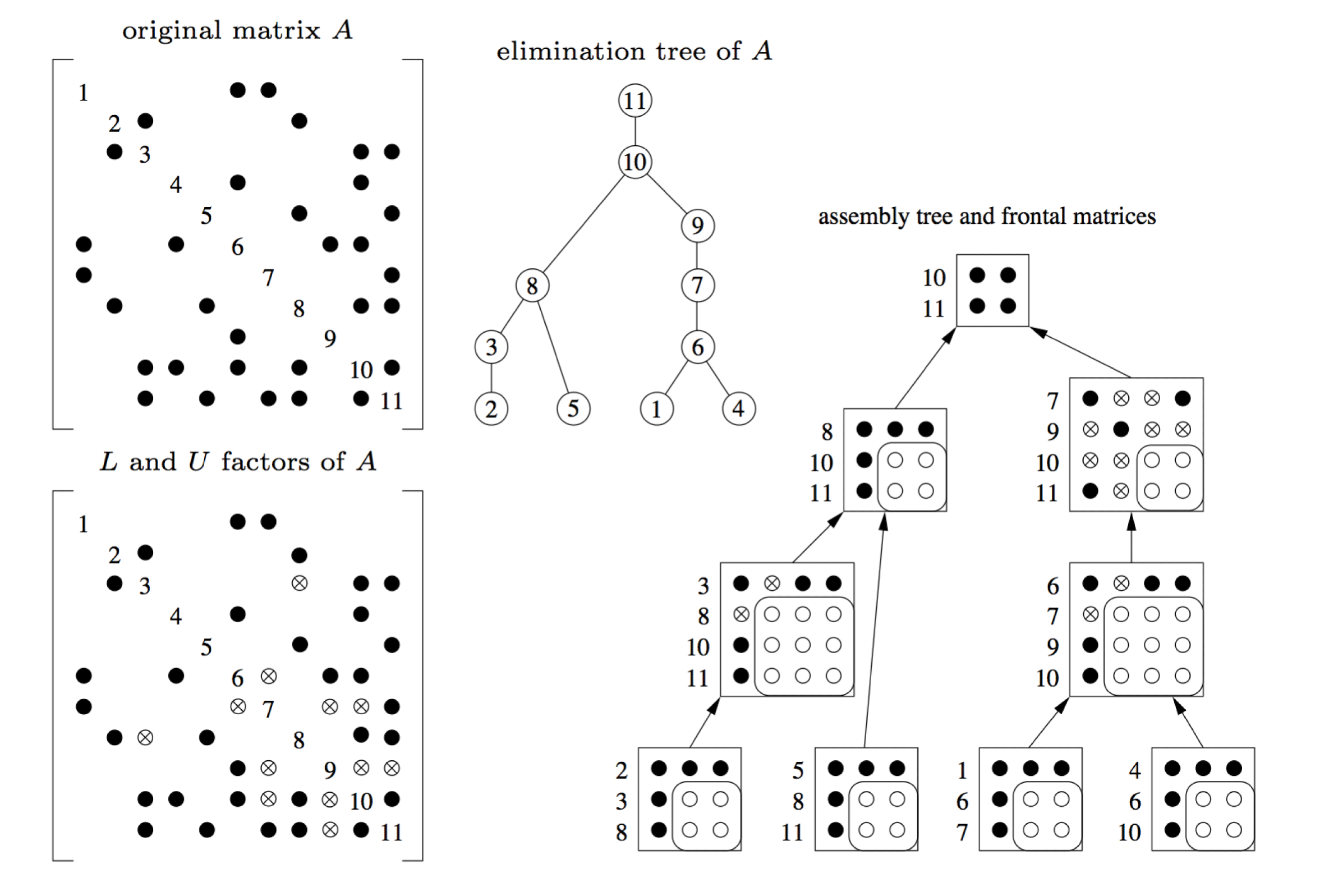
The frontal matrices are related to one another via the assembly tree, which is a coarser version of the elimination tree (some nodes having been merged together via amalgamation). To factorize a frontal matrix, the original entries of  $A$ are added, along with a summation of the contribution blocks of its children (called the assembly). One or more steps of dense LU factorization are performed within the frontal matrix, leaving behind its contribution block (the Schur complement of its pivot rows and columns). A high level of performance can be obtained using dense matrix kernels (the BLAS). The contribution block is placed on a stack, and deleted when it is assembled into its parent.
Figure 11.1 shows an assembly tree. Black circles represent the original entries of  $A$. Circled x’s represent fill-in entries. White circles represent entries in the contribution block of each frontal matrix. The arrows between the frontal matrices represent both the data flow and the parent/child relationship of the assembly tree.
A symbolic analysis phase determines the elimination tree and the amalgamated assembly tree. During numerical factorization, numerical pivoting may be required. In this case it may be possible to pivot within the fully assembled rows and columns of the frontal matrix. For example, consider the frontal matrix holding diagonal elements  $a_{77}$ and
 $a_{99}$ in Figure 11.1. If
 $a_{77}$ is numerically unacceptable, it may be possible to select
 $a_{79}$ and
 $a_{97}$ instead, as the next two pivot entries. If this is not possible, the contribution block of frontal matrix 7 will be larger than expected. This larger frontal matrix is assembled into its parent, causing the parent frontal matrix to be larger than expected. Within the parent, all pivots originally assigned to the parent and all failed pivots from the children (or any descendants) comprise the set of pivot candidates. If all of these are numerically acceptable, the parent contribution block is the same size as expected by the symbolic analysis.
The ordering has an important effect on the performance of the multifrontal method. Duff, Gould, Lescrenier and Reid (Reference Duff, Gould, Lescrenier, Reid, Cox and Hammarling1990) have studied the impact of minimum degree and nested dissection. They concluded that minimum degree induces very tall and thin trees while nested dissection induces short and large trees which thus express more parallelism. They also presented variants of the minimum degree ordering that aims at grouping the variables by similarity of their sparse structure to introduce more parallelism in the resulting elimination trees.
11.1.1 Exploiting dense matrix kernels
One of the key features of the multifrontal method is that it performs most of its computations inside dense submatrices. This allows for the use of efficient dense matrix kernels, such as dense matrix–matrix multiply (such as GEMM) and dense triangular solves (such as TRSM). Several studies have been made regarding how best to exploit these dense matrix kernels inside the multifrontal method.
Duff (Reference Duff, Handler, Haupt, Jeltsch, Juling and Lange1986b) discusses the inner parallelism arising in the computation of each individual front, known as node parallelism, together with the potential ways of exploiting it.
A first improvement to the efficiency of the multifrontal method is to avoid using the indirect addressing that usually arises in sparse matrix computations, as it is a bottleneck to efficiency, especially on vectorized computers.
Duff and Reid (Reference Duff and Reid1982) study three codes that use, in the innermost loop of the partial factorizations, full matrix kernels to avoid this indirect addressing of data and that exploit the vectorization feature of the Cray-1 computer. The three codes are: frontal unsymmetric (MA32), multifrontal symmetric (MA27), and a multifrontal out-of-core code for symmetric positive definite matrices.
Ashcraft (Reference Ashcraft1987) and Ashcraft et al. (Reference Ashcraft, Grimes, Lewis, Peyton and Simon1987) also propose ways of improving the efficiency of the multifrontal Cholesky method, particularly on vectorized supercomputers. Instead of relying solely on global indices to find the links between the variables of the sparse matrix and their location in the fronts, they propose the use of local indices in each front. An efficient assembly phase is then achieved through indexed vector operations, similar to the indexing scheme of Schreiber (Reference Schreiber1982) which allows for the use of vectorization. Schreiber (Reference Schreiber1982) describes a symmetric partial factorization of fronts using increased levels of vectorization. Instead of relying on single loops (vector–vector operations), he shows significant improvements when using supernode–node updates (multiple vector–vector operations) through unrolled double-loops, particularly when using supernode–supernode updates (multiple vector–multiple vector operations) via triple-loop kernels.
Ashcraft et al. (Reference Ashcraft, Grimes, Lewis, Peyton and Simon1987) rely on these ideas in studying and comparing highly vectorized supernodal implementations of both general sparse and multifrontal methods. They recognize that the uniform sparsity pattern of the nodes of a supernode provides a basis for vectorization, since all the columns in a supernode can be eliminated as a block. They conclude that these enhanced general sparse or multifrontal solvers are superior to band or envelope solvers in terms of execution time and storage requirements by orders of magnitude, and that the multifrontal method is more efficient than the general sparse method, at a cost of extra storage for the stack of contribution blocks and extra floating-point operations for assembly.
A second improvement to the efficiency of the multifrontal method is to use ideas from dense linear algebra, such as blocking strategies or use of BLAS or even of dense kernels, for the factorization of the (dense) fronts.
Rothberg and Gupta (Reference Rothberg and Gupta1993) show the effects of blocking strategies and the impact of cache characteristics on the performance of the left-looking, right-looking, and multifrontal approaches. They observe that: (1) column–column primitives (via Level 1 BLAS) yield low performance because of little data re-use, (2) supernode–column and column–supernode primitives (via Level 2 BLAS) can be unrolled, which allows data to be kept in registers and re-used, and (3) supernode-pair, supernode–supernode and supernode–matrix primitives (via Level 3 BLAS) allow the computations to be blocked, each one exploiting increasing amounts of data re-use until near saturation.
In sequential environments, Amestoy and Duff (Reference Amestoy and Duff1989) present an approach where they capitalize on the advances achieved in dense linear algebra, which are based on the use of block algorithms or BLAS, and implement their ideas as a modified version of MA37. In the assembly phase, they notice that when building the local indices, the index-searching operations for finding the position of a variable of a child in a parent can be very time-consuming. They thus introduce a working array that maps each variable of the child with either zero or the position of the corresponding variable in the parent front. During the factorization phase, to adapt the ideas of full matrix factorizations to partial front factorization, they try to maximize the use of Level 3 BLAS by dividing the computations into three steps. The fully summed rows are eliminated first, followed by an update of the non-fully summed part of the fully summed columns, through a blocked triangular solve, ending with an update of the Schur complement, using a matrix–matrix multiplication. The blocking strategy is further extended to the elimination of the fully summed rows by subdividing them into blocks, or panels, and applying vector operations inside the panels to eliminate their rows and blocked operations outside them to update the remaining fully summed rows. When pivots cannot be found inside a panel, it is merged with the next panel to increase the chance of finding a suitable pivot. They apply partial pivoting with column interchanges, which is allowed only within the pivot block. Such a restriction is leveraged by choosing a larger block size in case of failure to find a suitable pivot.
In parallel environments, Amestoy, Daydé and Duff (Reference Amestoy, Daydé, Duff, Delhaye and Gelenbe1989) extended these blocking ideas by proposing an approach where, instead of implementing a customized parallel LU factorization for each machine, which can be very efficient but not portable, they instead rely on a sequential blocked variant of the LU factorization that solely relies on parallel multithreaded BLAS (tuned for every machine) to exploit the parallelism of the machine. They show that this approach is portable and competitive in terms of efficiency, and adapted it to the partial factorization of frontal matrices.
Daydé and Duff (Reference Daydé, Duff, Palma and Dongarra1997) extend this approach of using off-the-shelf portable and efficient serial and parallel numerical libraries as building blocks for simplifying software development and improving reliability. They present the design and implementation of blocked algorithms in BLAS, used in dense factorizations and, in turn, in direct and iterative methods for sparse linear systems.
Duff (Reference Duff1996) also emphasizes the use of dense kernels, and particularly the use of BLAS, as portable and efficient solutions. He offers a review of the frontal and multifrontal methods.
Conroy, Kratzer, Lucas and Naiman (Reference Conroy, Kratzer, Lucas and Naiman1998) present a multifrontal LU factorization targeting large sparse problems on parallel machines with two-dimensional grids of processors. The method exploits a fine-grained parallelism solely within each dense frontal matrix, by eliminating each supernode, one at a time, using the entire processor grid. Parallel front assembly and factorization use low-level languages and minimize interprocessor communication.
It is possible to take even more advantage of dense matrix kernels by relaxing the fundamental supernode partition by means of node amalgamation. The idea is then to find a trade-off between obtaining larger supernodes and tolerating more fill-in, due to the introduction of logical zeros which increase the operation count and the storage requirement.
Duff and Reid (Reference Duff and Reid1983a) introduce this concept in their construction of a minimum degree ordering, to enhance the vectorization, by amalgamating variables corresponding to identical rows into a ‘supervariable’, in the same way as the indistinguishable nodes of George and Liu (Reference George and Liu1981). During a postorder traversal of the assembly tree, their heuristic consists in merging a supernode with the next one if the resulting supernode would be smaller than a user-defined amalgamation parameter.
Ashcraft and Grimes (Reference Ashcraft and Grimes1989) revisit the amalgamation approach to reduce the time spent in assembly, as Ashcraft (Reference Ashcraft1987) noticed that it takes a high percentage of the total factorization time. Their algorithm traverses, in a postorder, the assembly tree associated with the fundamental supernode partition (with no logical zeros). For each parent supernode, the largest children that add the fewest zeros are merged, one after another. The algorithm is controlled by a relaxation parameter that limits the additional fill-in. This approach leads to a reduction in the number of matrix assembly operations that were being performed in scalar mode, while increasing the number of matrix factorization operations that were being performed in vector mode, with only a slight reported increase in the total storage of the factors.
11.1.2 Parallelism via the elimination tree
Besides the parallelism offered by the Gaussian elimination process within each front, another source of parallelism is available in the multifrontal method.
Duff (Reference Duff1986a) describes the use of the elimination tree as an expression of the inner parallelism (now known as tree parallelism) arising in the multifrontal method. He considers a coarse-grained parallelism only when each task, consisting in the whole partial factorization of a front, can be treated by a single processor. The fundamental result he proves is that different branches or subtrees in the elimination tree can be treated independently and in parallel. The elimination tree can be interpreted as a partial order on the tasks. Leaves can be processed immediately and sibling fronts or subtrees can be treated in any order and in parallel; whereas parent tasks may be activated only after all their child tasks complete. He then shows how to schedule and synchronize tasks among processors accordingly, in parallel shared- and distributed-memory environments.
Duff (Reference Duff, Handler, Haupt, Jeltsch, Juling and Lange1986b) extends this study by showing how to interleave both tree and node parallelism during the multifrontal factorization. He starts from the observation of Duff and Johnsson (Reference Duff, Johnsson and Carey1989) that the shape of the elimination tree provides fronts that are abundant and small near the leaves, but that decrease in number and grow in size towards the root. Duff (Reference Duff, Handler, Haupt, Jeltsch, Juling and Lange1986b) thus proposes to benefit from the natural advantages of each kind of parallelism wherever available, that is, to use tree parallelism near the leaves and then progressively move towards node parallelism near the root.
Both node and tree parallelism may be exploited in both shared- and distributed-memory environments. This will be the subject of the two following sections.
11.1.3 Shared-memory parallelism
Benner, Montry and Weigand (Reference Benner, Montry and Weigand1987) propose a parallel approach that relies on the use of nested dissection, for its inherent separation of finite element dependencies, to reduce communication and synchronization, thus improving parallel and sequential performance. Their algorithm and implementation use distributed-memory paradigms while targeting shared-memory machines.
Duff (Reference Duff1989b) presents the approach of designing and implementing a parallel solver from a serial one, through a modified version of MA37 on shared-memory systems. He uses node parallelism, over blocks of rows on large enough fronts, in addition to tree parallelism. He defines static tasks on the tree level, corresponding to assembly, pivoting, storage of factors and stacking of contribution blocks, together with dynamic tasks, corresponding to the elimination operations. He manages the computations using a single work queue of tasks and explains how these tasks are identified and put in / pulled from the queue. He then shows the effect of synchronization and implementation on efficiency. He also presents a precursor use of a runtime system (the SCHEDULE package by Dongarra and Sorensen) in a multifrontal solver. He highlights that the natural overhead of such general systems incurs performance penalties over a direct implementation of the code.
Kratzer and Cleary (Reference Kratzer, Cleary, George, Gilbert and Liu1993) target the communication overhead and load balancing issues arising in the factorization of matrices with unstructured non-regular sparsity patterns. They implement a dataflow paradigm on MIMD and SIMD machines relying on supernodes and elimination trees.
Irony, Shklarski and Toledo (Reference Irony, Shklarski and Toledo2004) design and implement a recursive multifrontal Cholesky factorization in shared-memory. Their approach relies on an aggressive use of recursion and the simultaneous use of recursive data structures, automatic kernel generation, and parallel recursive algorithms. Frontal matrices are laid down in memory based on a two-dimensional recursive block partitioning. Block operations are performed using novel optimized BLAS and LAPACK kernels (Anderson et al. Reference Anderson, Bai, Bischof, Blackford, Demmel, Dongarra, Du Croz, Greenbaum, Hammarling, Mckenney and Sorensen1999), which are produced through automatic kernel generators. The use of recursion allows them to use Cilk as a parallelization paradigm. They apply a sequential postorder traversal of the elimination tree where Cilk subroutines are spawned and synchronized on the factorization and assembly of each front.
L’Excellent and Sid-Lakhdar (Reference L’Excellent and Sid-Lakhdar2014) adapt a multifrontal distributed-memory solver to hybrid shared- and distributed-memory machines. Instead of relying solely on multithreaded BLAS to take advantage of the shared-memory parallelism, they introduce a layer in the tree under which subtrees are treated by different threads, while all threads collaborate on the treatments above the layer. They propose a memory management scheme that takes advantage of NUMA architectures. To leverage the heavy synchronization incurred by the separating layer, they propose an alternative to work-stealing that allows idle processors to be re-used by active threads.
11.1.4 Distributed-memory parallel Cholesky
We now discuss techniques developed for the multifrontal Cholesky method, where the exact structure of the tree and the exact amounts of computations are known in advance, prior to the factorization phase.
The communication characteristics and behaviour of the Cholesky multifrontal method in distributed-memory environments have been thoroughly studied.
Ashcraft et al. (Reference Ashcraft, Eisenstat, Liu and Sherman1990b) compare the distributed fan-out, fan-in, and multifrontal algorithms for the solution of large sparse symmetric positive definite matrices. They highlight the communication requirements and relative performance of the different schemes in a unified framework abstracting from any implementation. Then, using their implementations, they conclude that the multifrontal method is more efficient than the fan-in schemes (which are more efficient than the domain fan-out scheme), although it requires more communication.
Eswar et al. (Reference Eswar, Sadayappan, Visvanathan, Özgüner and Erçal1993a) present a similar study with similar results. They show the impact of the mapping of columns of a matrix to processors and show significant reduction of communication in the multifrontal method on networks with broadcast capabilities.
Lin and Chen (Reference Lin and Chen2000) have the same objective but target the lack of theoretical evaluations of the performance of the multifrontal method that is due to the irregular structure involved in its computations. They thus compare column-Cholesky, row-Cholesky, submatrix-Cholesky and multifrontal methods from a theoretical standpoint by relying on the elimination tree model, and conclude the superiority of the last one.
The ordering that is chosen and the resulting shape of the elimination tree has an important impact on parallelism.
For instance, Lucas, Blank and Tiemann (Reference Lucas, Blank and Tiemann1987) present a processor mapping for a distributed multifrontal method, precursor to the subtree-to-subcube mapping by George et al. (Reference George, Heath, Liu and Ng1989a). Their mapping is designed with the minimization of communications overhead in mind. In a top-down phase, they create the elimination tree at the same time as they map the processors by partitioning the sparse matrix using the nested dissection ordering and by assigning processors of separate sub-networks to different subdomains or subtrees of the elimination tree, until a subdomain is isolated for every processor. Each processor may then apply local orderings, assemblies and eliminations on its sparse submatrix, without communicating with other processors. Then, in a bottom-up phase, the processors of the same subcube collaborate for the elimination of their common separator, limiting the communications to the subcube. Hence Lucas et al. (Reference Lucas, Blank and Tiemann1987) show significant reduction of communication compared to previous approaches.
Similarly, Geng, Oden and van de Geijn (Reference Geng, Oden and van de Geijn1997) show the effectiveness of the use of the nested dissection ordering in the multifrontal method while leveraging the implementation issues related to such an approach. They also present performance results on two- and three-dimensional finite element and difference problems.
Heath and Raghavan (Reference Heath and Raghavan1997) describe the design and the development of CAPSS for sparse symmetric positive definite systems on distributed-memory computers. Their main idea is to break each phase into a distributed phase, where processors communicate and cooperate, and a local phase, where processors operate on an independent portion of the problem.
Besides the shape of the tree, an appropriate mapping of the elimination tree on the processes is a key to efficiency.
Gilbert and Schreiber (Reference Gilbert and Schreiber1992) give a highly parallel multifrontal Cholesky algorithm. A bin-packing mapping strategy is used to map a two-dimensional grid of processors (of the Connection Machine) on several simultaneous fronts factorizations. They rely on an efficient fine-grained parallel dense partial factorization algorithm.
Gupta et al. (Reference Gupta, Karypis and Kumar1997) present a scalable multifrontal Cholesky algorithm. It relies on the subtree-to-subcube assignment strategy, and in particular, on a two-dimensional block cyclic distribution of the frontal matrices that helps to maintain a good load-balancing and reduces the assembly communications. An implementation of this algorithm is presented by Joshi et al. (Reference Joshi, Karypis, Kumar, Gupta, Gustavson and Yang1999) in the PSPASES package. They incorporated the parallel ordering algorithm they use in the ParMetis library.
Such subtree-to-subcube-like mappings are adequate on regular problems but not on irregular problems, where the elimination tree is unbalanced. Pothen and Sun (Reference Pothen and Sun1993) present the proportional mapping in a distributed multifrontal method. It may be viewed as a generalization of the subtree-to-subcube mapping of George et al. (Reference George, Heath, Liu and Ng1989a) in which both the structure and the workload are taken into account. The objective of Pothen and Sun is to achieve a good load balance and a low communication cost while targeting irregular sparse problems. Inspired by the work of Gilbert and Schreiber (Reference Gilbert and Schreiber1992) and Geist and Ng (Reference Geist and Ng1989), they traverse the elimination tree in a top-down manner, using a first-fit-decreasing bin-packing heuristic on the subtrees to assign them to the processors, replacing the heaviest subtree by its children and repeating the process until a good balance between the processors is obtained.
11.1.5 Distributed-memory parallel $\text{LDL}^{\text{T}}$ and LU factorization

We now discuss the techniques targeting distributed-memory multifrontal  $\text{LDL}^{\text{T}}$ and LU factorizations, where the unpredictability of the numerical pivoting has an influence on the load balance of the computations, and thus involve different sets of strategies.
Amestoy, Duff and L’Excellent (Reference Amestoy, Duff and L’Excellent2000) and Amestoy, Duff, L’Excellent and Koster (Reference Amestoy, Duff, L’Excellent and Koster2001a) present a fully asynchronous approach with distributed dynamic scheduling. They based their resulting distributed-memory code MUMPS on the shared-memory code MA41. They target symmetric positive definite, symmetric indefinite, unsymmetric, and rank-deficient matrices.
Asynchronous communications are chosen to enable overlapping between communication and computation. The message transmission and reception mechanisms are carefully used to avoid the related distributed synchronization issues. In the main loop of their algorithm, processes treat untreated messages if any, and otherwise activate tasks from a pool.
In contrast to other approaches relying on static pivoting and iterative refinement to deal with numerical difficulties, the numerical strategy they propose is based on partial threshold pivoting together with delayed pivoting in distributed-memory. The Schur complements thus become dynamically larger than anticipated, as they contain the numerically unstable fully summed rows and columns. Dynamic scheduling was initially used to accommodate this unpredictability of numerical pivoting in the factorizations. However, guided by static decisions during the analysis phase, it has been further exploited for the improvement of computation and memory load balancing.
Both tree parallelism and node parallelism are exploited through three types of parallelism. In type 1 parallelism, fronts are processed by a single processor. The factorization kernels use right-looking blocked algorithms that rely heavily on Level 3 BLAS kernels. In type 2, a one-dimensional block partitioning of the rows of the fronts is applied. The fully summed rows are assigned to a master process that handles their elimination and numerical pivoting, and the contribution block rows are partitioned over slave processes that handle their updates. In type 3, a two-dimensional block-cyclic partitioning is applied to the root front through the use of ScaLAPACK (Blackford et al. Reference Blackford, Choi, Cleary, D’Azevedo, Demmel, Dhillon, Dongarra, Hammarling, Henry, Petitet, Stanley, Walker and Whaley1997). A static mapping of the assembly tree to the processors is determined using a variant of the proportional mapping and the Geist and Ng (Reference Geist and Ng1989) algorithm that balances both computation and memory requirements of the processors.
Amestoy, Duff, Pralet and Vömel (Reference Amestoy, Duff, Pralet and Vömel2003b) revisit both their static and dynamic scheduling algorithms to address clusters of shared-memory machines. Their first strategy relies on taking into account the non-uniform cost of communications on such heterogeneous architectures. To prevent the master process (of type 2 fronts) from doing expensive communications, their architecture-aware algorithm penalizes the current workload of processes which are not on the same SMP node as the master, during its dynamical determination of the number and choice of slave processes. Their second strategy relies on a hybrid parallelization, mixing the use of MPI processes (distributed-memory) with the use of OpenMP threads (shared-memory) inside each process. The scalability limitations of the one-dimensional block partitioning among processes is traded over a pseudo-two-dimensional block partitioning among threads. This allows for a decrease in the communication volume and the use of multithreaded BLAS.
Amestoy, Duff and Vömel (Reference Amestoy, Duff and Vömel2004b) further address scalability issues using the candidate-based scheduling idea, an intermediate step between fully static and fully dynamic scheduling. Where the master (of a type 2 front) was previously free to choose slaves dynamically among all (less loaded) processors, it now chooses them solely from a limited set of candidate processors. The choice of this list of candidates is guided by static decisions during the analysis phase that accounts for global information on the assembly tree. This leads to localized communications, through a more subtree-to-subcube-like mapping, and to more realistic predictions than the previous overestimates for memory requirement of processes’ workspaces.
Amestoy, Guermouche, L’Excellent and Pralet (Reference Amestoy, Guermouche, L’Excellent and Pralet2006) improve their scheduling strategy for better memory estimates, lower memory usage, and better factorization times. Their previous strategy resulted in an improved memory behaviour but at the cost of an increase in the factorization time. Their new idea is to modify their original static mapping to separate the elimination tree into four zones, where they apply a relaxed proportional mapping in zone 1 (near the root), strict proportional mapping in zone 2, fully dynamic mapping in zone 3, and (unmodified) subtree-to-process mapping in zone 4 (near the leaves).
Amestoy, L’Excellent, Rouet and Sid-Lakhdar (Reference Amestoy, L’Excellent, Rouet and Sid-Lakhdar2014b) propose improvements to the one-dimensional asynchronous distributed-memory dense kernels algorithms to improve the scalability of their multifrontal solver. They notice that, in a left-looking approach, the master process produces factorized panels faster at the beginning than at the end of its factorization, thus resulting in improved scheduling between master and slaves. This contrasts with a right-looking approach, which prohibits the slave processes from being starved at the beginning and overwhelmed at the end of their update operations. They also notice that the communication scheme is a major bottleneck to the scalability of their distributed-memory factorizations. They then proposed an asynchronous tree-based broadcast of the panels from the master to the slaves.
Amestoy, L’Excellent and Sid-Lakhdar (Reference Amestoy, L’Excellent and Sid-Lakhdar2014a) further notice that, although greatly improving the communication performance, this broadcast scheme breaks the fundamental properties on which they were relying to ensure deadlock-free factorizations. They then propose adaptations of deadlock prevention and avoidance algorithms to the context of asynchronous distributed-memory environments. Relying on these deadlock-free solutions, they further characterize the shape of the broadcast trees for enhanced performance.
Amestoy et al. (Reference Amestoy, Duff, L’Excellent and Li2001b) compare their two distributed-memory approaches and software: SuperLU_DIST, which relies on a synchronous supernodal method with static pivoting and iterative refinement (discussed in Section 9.2), and MUMPS, which uses an asynchronous multifrontal method with partial threshold and delayed pivoting.
Amestoy et al. (Reference Amestoy, Duff, L’Excellent and Li2003a) report their experience of using MPI point-to-point communications on the performance of their respective solvers. They present challenges and solutions on the use of buffered asynchronous message transmission and reception in MPI.
Finally, Kim and Eijkhout (Reference Kim and Eijkhout2014) present a multifrontal LU factorization over a DAG-based runtime system. They rely on a hierarchical representation of the DAG that contains the scheduling dependencies of both the fronts factorization (dense level) and the elimination tree (sparse level).
11.2 Numerical pivoting for LDL and symmetric-structure LU factorization
The main problem with multifrontal methods when numerical pivoting is required is that it might not be possible to find a suitable pivot within the fully summed block of the frontal matrix. If this is the case then the elimination at that node of the tree cannot be completed and a larger Schur complement (or contribution block) must be passed to the parent node in the elimination tree. This means that the data structures will change from that determined by the analysis, and dynamic structures will be required.
This phenomenon is introduced by Duff and Reid (Reference Duff and Reid1983a) and is termed delayed pivoting. It will normally result in more storage and work for the factorization. The need for dynamic pivoting also greatly complicates the situation particularly for parallel computation.
Liu (Reference Liu1988b) highlights the importance of delayed pivoting in the multifrontal method. He provides a quantitative upper bound on the increase of fill-in it induces in the resulting triangular factors. He also observes that delayed pivoting occurring within a subtree does not affect parts of the elimination tree outside this subtree.
11.2.1 2 $\times$ 2 pivoting for indefinite matrices

The methods we discuss now target sparse symmetric indefinite matrices and consider sparsity and numerical stability.
Duff, Reid, Munksgaard and Nielsen (Reference Duff, Reid, Munksgaard and Nielsen1979) adapt ideas used in the dense case to the case of sparse symmetric matrices. They consider the use of  $2\times 2$ pivots in addition to the standard
 $1\times 1$ pivots. They show that this strategy permits a stable factorization in the indefinite case and incurs only a small performance loss, even in the positive definite case. They propose a numerical stability condition for
 $2\times 2$ pivots and extend the Markowitz strategy to the indefinite case, defining a generalized Markowitz cost (sparsity cost) for
 $2\times 2$ pivots. Potential
 $2\times 2$ pivots are chosen over potential
 $1\times 1$ pivots if their sparsity cost is less than twice that of the best
 $1\times 1$ pivot, although
 $1\times 1$ pivots are favoured in the absence of stability problems.
Liu (Reference Liu1987e) explores the use of a variant of threshold partial pivoting strategy in the multifrontal method. His algorithm restricts the search space for stable  $1\times 1$ and
 $2\times 2$ pivots to the submatrix of fully summed rows and columns of the front. However, it compares the largest off-diagonal entry in the fully summed part of a front with the largest off-diagonal entry in the whole candidate row of the front. If no suitable pivot can be found, a delayed pivoting strategy is applied instead. Liu shows that this strategy is as effective as that originally used by Duff and Reid.
Liu (Reference Liu1987d) further proposes a relaxation of the original threshold condition of Duff and Reid which is nearly as stable. Instead of using the same threshold parameter  $u$ for both the
 $1\times 1$ and
 $2\times 2$ pivot conditions, he defines a different parameter for each pivot condition, with a smaller threshold for
 $2\times 2$ than for
 $1\times 1$ pivots. He then extends the range of permissible threshold values for
 $2\times 2$ pivots from
 $[0,{\textstyle \frac{1}{2}})$ to
 $[0,u)$, with
 $u$ defined as
 $$\begin{eqnarray}\frac{1+\sqrt{17}}{8}\quad ({\approx}0.6404),\end{eqnarray}$$
allowing for a broader choice of block  $2\times 2$ pivots.
Instead of using pivoting strategies to avoid zero diagonal entries, Duff et al. (Reference Duff, Gould, Reid, Scott and Turner1991) introduced pivoting strategies that take advantage of them. They introduce oxo and tile pivots, which are new kinds of  $2\times 2$ pivots with a structure that contains zeros on their diagonals. The advantage is that their elimination involves fewer operations than the usual full pivots as it preserves a whole block of zeros. Duff et al. study strategies to use such
 $2\times 2$ pivots not only during the factorization phase but also during the analysis phase, and apply their ideas in a modification of MA27. After trying to extend the minimum degree ordering to the inclusion of such pivots, they prefer to consider the use of
 $1\times 1$ and oxo pivots in a variant of the strategy of Markowitz (1957) as an alternative. The algorithms developed have been implemented and their results discussed by Duff and Reid (Reference Duff and Reid1996b).
Ashcraft, Grimes and Lewis (Reference Ashcraft, Grimes and Lewis1998) present algorithms for the accurate solution of symmetric indefinite systems. Their main objective is to bound the entries in the factor  $L$. To this effect, they propose two algorithms for the dense case, namely, the bounded Bunch–Kaufman and the fast Bunch–Parlett algorithms, and show that the cost for bounding
 $|L|$ is minimal in this case. They then propose strategies in the sparse case to find large
 $2\times 2$ pivots, based on the strategies of Duff and Reid (Reference Duff and Reid1983a) and Liu (Reference Liu1987e), resulting in faster and more accurate strategies.
Duff and Pralet (Reference Duff and Pralet2005) present a scaling algorithm together with strategies to predefine  $1\times 1$ and
 $2\times 2$ pivots through approximate symmetric weighted matchings and before the ordering phase. They further use the resulting information to design the classes of (relaxed) constrained orderings that then use two distinct graphs to get structural and numerical information respectively. Weighted matching and scaling is an important topic in its own right, and is considered in more detail below.
Schenk and Gärtner (Reference Schenk and Gärtner2006) combine the use of numerical pivoting and weighted matching. To avoid delayed pivoting in the presence of numerical difficulties, to keep the data structures static, they use a variant of Bunch and Kaufman’s (Reference Bunch and Kaufman1977) pivoting strategy, which restricts the choice of  $1\times 1$ and
 $2\times 2$ pivots to the supernodes. To reduce the impact on numerical accuracy imposed by this pivoting restriction, they supplement their method with pivot perturbation techniques and introduce two strategies, based on maximum weighted matchings, to identify and permute large entries of the coefficient matrix close to the diagonal, for an increased potential of suitable
 $2\times 2$ pivots.
Duff and Pralet (Reference Duff and Pralet2007) present pivoting strategies for both sequential and parallel factorizations. For sequential factorizations, they describe a pivoting strategy that combines numerical pivoting with perturbation techniques followed by a few steps of iterative refinement, and compare it with the approach by Schenk and Gärtner (Reference Schenk and Gärtner2006). They also show that perturbation techniques may be beneficial when combined with static pivoting but dangerous when combined with delayed pivoting, as the influence of diagonal perturbations on rounding errors may contaminate pivots postponed to ancestor nodes instead of being localized to the contribution block of the current front. For parallel distributed-memory factorizations, they propose an approach that allows the process that takes the numerical pivoting decisions on a parent front to have an approximation of the maximum entry in each fully summed column, by sending to it the maximum entries of the contribution blocks of the child fronts.
Duff (Reference Duff2009) targets the special case of sparse skew-symmetric matrices, where  $A=-A^{T}$. He considers an
 $\text{LDL}^{\text{T}}$ factorization of such matrices, taking advantage of their specific characteristics to simplify the usual pivoting strategies. He then shows the potential of this factorization as an efficient preconditioner for matrices containing skew components.
In the context of an out-of-core multifrontal method, delayed pivoting causes additional fill-in to occur in the factors, leading to an increase of input/output operations. Scott (Reference Scott2010) targets this issue by examining the impact of different scaling and pivoting strategies on the additional fill-in. After considering threshold partial pivoting, threshold rook pivoting, and static pivoting, she concludes the importance of scaling and the potential benefits of rook pivoting over partial pivoting for factorization time and memory requirements.
When the problem is numerically challenging, Hogg and Scott (Reference Hogg and Scott2013d) target a reduction in the significant amount of delayed pivoting arising from the factorization. To this end, they propose a review of different pivoting strategies and give recommendations on their use. They also present constrained and matching-based orderings, during the analysis phase, for the preselection of potentially stable  $2\times 2$ pivot candidates.
11.2.2 Weighted matching and scaling
It is possible to help the pivoting strategies by increasing their chances of finding satisfiable pivots on or near the diagonal. This is the main purpose of the weighted matching and scaling techniques. This family of techniques is similar but differs from the techniques presented in Section 8.7.2, in that techniques presented in that section consider only the non-zero structure of the sparse matrix while the weighted matchings also consider the numerical values of the entries. A survey of the work that has been achieved on scaling and matching algorithms for sparse matrices is presented by Duff (Reference Duff2007).
Duff and Koster (Reference Duff and Koster1999) introduce the concept of weighted matching on sparse matrices inspired by the work of Olschowka and Neumaier (Reference Olschowka and Neumaier1996) on dense unsymmetric matrices. A maximal weighted matching is a permutation of a matrix that leads to large absolute entries on the diagonal of the permuted matrix. To find such matchings, Duff and Koster present the bottleneck transversals algorithm. It aims at maximizing the smallest value on the diagonal of the permuted matrix, and relies on the repeated application of the depth-first search algorithm MC21, which operates on unweighted bipartite graphs to put as many entries as possible onto the diagonal. They also present maximum product transversals, which they further extend and explain in a subsequent paper (Duff and Koster Reference Duff and Koster2001) and which is based on the strategy of Olschowka and Neumaier (Reference Olschowka and Neumaier1996). This algorithm consists in maximizing the product of the moduli of the entries on the diagonal. It is based on obtaining a minimum weighted bipartite matching of a graph through a sequence of augmented (shortest) paths used to extend a partial matching. Duff and Koster (Reference Duff and Koster2001) show the influence and importance of scaling, and propose a variant of the algorithm by Olschowka and Neumaier that scales so that the diagonal entries have a value of 1.0 and smaller off-diagonal entries. They also show the benefits of the scaling and matching preprocessings for the numerical stability and efficiency of direct solvers and preconditioners for iterative methods.
Based on this work and that of Duff and Pralet (Reference Duff and Pralet2005), Hogg and Scott (Reference Hogg and Scott2013c) introduce an algorithm for optimal weighted matchings of rank-deficient matrices. They apply a preprocessing to the matrix that aims to retain the symmetry of the matrix before modifying it to handle its potential structural rank-deficiency. They show that their algorithm has some overheads but that it improves the quality of the matchings on some matrices.
11.3 Memory management
Duff and Reid (Reference Duff and Reid1983a) present a memory management scheme for the multifrontal method in the sequential context. The main difference between the multifrontal and frontal methods is that in the multifrontal method, contribution blocks are generated but not consumed immediately by the next front, which requires them to be stored temporarily for future consumption. Given the relative freedom in the traversal of the elimination tree, Duff and Reid propose the use of a postorder. The stack storage mechanism is then an adapted data structure for holding the contribution blocks, as its first-in/last-out scheme fits the order of generation and consumption obtained. After each front factorization, the resulting contribution blocks are stacked, and during the assembly of each front, the contribution blocks it needs to consume are then located on top of the stack from which they are popped out.
The multifrontal memory management in a sequential context relies on one main large workspace, organized as follows. A stack is used to store the factors, starting at the left of the workspace and growing to the right. A region is used to store the original rows of the sparse matrix (in element, arrowhead, or other format), at the right of the workspace. Another stack stores the contribution blocks at the left of the region containing the original rows and growing to the left towards the stack of factors. An active area is used to hold the frontal matrices, whose location differs depending on the front allocation strategy.
Two main front allocation strategies exist. The fixed-front approach allocates one area of the size of the largest front, to hold all the frontal matrices. It is similar to the approach of Irons (Reference Irons1970) in the frontal method. The dynamically allocated front approach allocates a fresh area for each front. It is adopted by Duff and Reid (Reference Duff and Reid1983a) as they observe that the size of the different fronts varies greatly in the multifrontal method. They also propose a variant known as the in-place strategy. It consists in overlapping the allocation of a parent front with its child’s contribution that is on top of the contribution stack.
Duff (Reference Duff1989b) shows that the data management scheme in the sequential case is not suitable for parallel execution. He discusses different schemes for the parallel context, emphasizing on synchronization issues, waste of free space and garbage collection, fragmentation and locality of data. He then selects the buddy system (i.e., blocks of size  $2^{i}$) and fixed blocks allocation strategies.
Following this work, Amestoy and Duff (Reference Amestoy and Duff1993) propose an adaptation and extension of the sequential memory management to the (shared-memory) parallel context. They favour the (static) fixed-front allocation scheme, as the large active area they allocate may then accommodate the storage of several active frontal matrices that are factorized in parallel. Due to the varying number and size of these fronts, the allocation strategy they adopt for this area is a mixture of the fixed blocks and buddy system strategies, as advised by Duff (Reference Duff1989b). Moreover, since the traversal of the elimination tree in parallel is no longer a postorder, the stack of contributions grows more than in the sequential case and free spaces appear inside it, due to the unpredictable consumption of the contributions. They thus use a garbage collection mechanism for the stack, known as compress. The compress consists in compressing the contribution blocks to the bottom (right) of the stack to re-use the free spaces it contains. This idea is also present in the work of Ashcraft (Reference Ashcraft1987), as an alternative to the systematic stacking of the contribution blocks, where the contributions are left unstacked after each front factorization, and where a compress is applied only when the workspace is filled. Amestoy and Duff also propose a strategy to keep some contributions inside the active area if their stacking would require such a garbage collection.
11.3.1 In-core methods
In an in-core context, the factors, contribution blocks and fronts are all held in core memory during the factorization phase.
Sparse direct methods are known to require more memory than their iterative counterparts. The multifrontal method is also known to consume more memory than its frontal or supernodal counterparts, mainly due to the storage of contribution blocks. However, Duff and Reid (Reference Duff and Reid1983a) notice that the storage and arithmetic requirements of the multifrontal factorization can be predicted, in the absence of numerical pivoting considerations. The order of the traversal of the elimination tree has a deep impact on the average and maximum memory used during the factorization phase.
In the sequential case, the choice of the postorder traversal by Duff and Reid (Reference Duff and Reid1983a) helps to reduce the memory usage. They attempted to improve it by ordering the children of a parent node by increasing order of their size from the left to the right. Their hope was that the large rightmost contributions will be consumed sooner, reducing the growth of the stack. They found this strategy ineffective, however.
Liu (Reference Liu1986d) proposes a solution to this problem with his child reordering variant, with respect to the maximum in-core storage required (factors and stack). He determines a simple and optimal order of the children, based not only on their size but also on the memory required for treating the subtrees for which they are the root. This strategy is extended by Ashcraft (Reference Ashcraft1987) to the case of the supernode elimination tree, where many pivots are eliminated at each node, and who also notices the impact of the in-place strategy (called sliding) on the reduction in memory. Liu (Reference Liu1986d) also proposes a variant of the in-place strategy, where the parent is pre-allocated before the factorization of its children begin, so that their contribution blocks are directly assembled in it, without being stacked. Although the strategy proved to be disappointing in the general case, he highlighted its potential for particular cases.
Indeed, instead of relying on this pre-allocation or the standard post-allocation, Guermouche and L’Excellent (Reference Guermouche and L’Excellent2006) propose an intermediate strategy where the parent may be allocated after any number of children have already been factorized. Child contributions are stored in the stack before its allocation, while they are directly assembled in it after its allocation. Guermouche and L’Excellent then propose two tree traversals that take advantage of this allocation flexibility and that target, respectively, the in-core and out-of-core contexts.
Guermouche, L’Excellent and Utard (Reference Guermouche, L’Excellent and Utard2003) show the effect of reordering techniques on stack memory usage. They observe that orderings based on nested dissection yield wide balanced elimination trees, which increase the stack usage, while local orderings yield deep unbalanced trees, which help to decrease the stack usage. They also propose two variants of the algorithm by Liu (Reference Liu1986d) that target the minimization of the global memory (both stack and factors) and average stack size respectively. They then show that, in the parallel distributed-memory case, the stack memory does not scale ideally, and they present ideas to target this issue.
11.3.2 Out-of-core methods
In an out-of-core context, to target larger problems whose factorization would require more core memory than is available, secondary storage media (such as disks) are exploited by allowing the factors and/or contribution blocks to be stored on them during the factorization phase. Contribution blocks, if stored, are retrieved into core memory for their assembly, while factors are retrieved only during the solution phase.
Ashcraft et al. (Reference Ashcraft, Grimes, Lewis, Peyton and Simon1987) study out-of-core schemes in the frontal and multifrontal methods based on the algorithm of Liu (Reference Liu1987a) on sparse Cholesky factorizations. The main idea of Liu is that, once a variable has been eliminated (and used to update the remainder of the system), its factors are no longer used during the factorization process. It may then be stored on disk for future use during the solution phase. Ashcraft et al. also factorize and store supernodes instead of single variables.
Liu (Reference Liu1989c) shows the advantage of the multifrontal method over the sparse column-Cholesky method in terms of memory traffic on a paged virtual memory system. He then extends the idea of switching from sparse to dense kernels. He introduces a hybrid factorization scheme that switches back and forth from multifrontal to sparse column-Cholesky schemes. More specifically, this method uses a multifrontal scheme for its reduced memory traffic and a sparse scheme when constraints arise on the amount of available core memory.
Rothberg and Schreiber (Reference Rothberg and Schreiber1999) synthesize the multifrontal and supernodal methods into a hybrid method for their out-of-core sparse Cholesky factorization. The matrix splits into panels; each panel is a supernode or part of a supernode, where no panel is larger than 1/2 of available memory. The multifrontal method requires less I/O to disk than the left-looking supernodal method, but it requires more in-core memory. Thus, it is used for subtrees, for which the contribution stack can be held in core. The remainder of the matrix (towards the top of the assembly tree) is factorized with a left-looking method. Rothberg and Schreiber consider two variants of this hybrid method. In the first, the contribution block of the root of each subtree remains in core; in the second, it is written to disk.
Cozette, Guermouche and Utard (Reference Cozette, Guermouche and Utard2004) present a way of modifying an in-core solver into an out-of-core solver seamlessly. They rely on a modification of the low-level paging mechanisms of the system to make the I/O operations become transparent. They make two observations: factors are not read back during the factorization and can thus be written to disk whenever possible; contribution blocks at the bottom of the stack are more likely to stay in it for longer, making their memory pages better candidates for eviction to disk in case of memory difficulties. They then rely on these observations to design an appropriate memory paging policy.
Agullo, Guermouche and L’Excellent (Reference Agullo, Guermouche and L’Excellent2008) show the improvements in efficiency of an out-of-core solver when shortcutting the buffered system level I/O mechanisms, by use of direct disk accesses to store the factors. Based on an out-of-core solver that stores only the factors on disk, they study the additional benefits of storing the contribution blocks as well. They present different storage schemes of the contribution blocks and their corresponding memory reductions. They conclude that the best strategy is to allow the flexibility of storing all the contribution blocks on disk, if needed.
Agullo, Guermouche and L’Excellent (Reference Agullo, Guermouche and L’Excellent2010) further show that the reduction in the available in-core memory induces increases in the volume of I/O. Thus, they present a postorder traversal of the tree that aims at reducing the volume of I/O (MinIO) instead of the amount of memory (MinMEM). Then, to reduce the memory requirements, they revisit different variants of the flexible parent allocation scheme by Guermouche and L’Excellent (Reference Guermouche and L’Excellent2006), namely, the classical, last-in-place and max-in-place variants, and present their impact on both memory and I/O.
Reid and Scott (Reference Reid and Scott2009a, Reference Reid and Scott2009b) discuss the design and implementation of the MA77 and MA78 packages for the out-of-core solution of symmetric and unsymmetric matrices, respectively. They rely on the use of a custom virtual-memory system that allows the data to be spread over many disks. This enables them to solve large sparse systems.
The availability of the out-of-core feature in a solver may be exploited to perform numerical tasks other than solving a system. Indeed, Amestoy et al. (Reference Amestoy, Duff, L’Excellent, Robert, Rouet and Uçar2012) propose heuristics to efficiently compute entries of the inverse of a sparse matrix, in an out-of-core environment. Their algorithms are based on techniques similar to that used in the solution phase of the multifrontal method when the right-hand sides are sparse. To access only parts of the factors, and thus to minimize the amount of accesses to the disks, they show that it is possible to (1) prune the elimination tree to select only specific paths between nodes and the root, and (2) partition the requested inverse entries into blocks based on the set of factors they require in common. Amestoy, Duff, L’Excellent and Rouet (Reference Amestoy, Duff, L’Excellent and Rouet2015b) extend this work further to a distributed-memory context, showing that parallelism and computation throughput are different criteria for this kind of computation.
11.4 Unsymmetric-structure multifrontal LU factorization
If the non-zero pattern of  $A$ is unsymmetric, the frontal matrices become rectangular. They are related either by the column elimination tree (the elimination tree of
 $A^{T}A$) or by a DAG, depending on the method. An example is shown in Figure 11.2.
This is the same matrix used for the QR factorization example in Figure 7.1. Using a column elimination tree, arbitrary partial pivoting can be accommodated without any change to the tree. The size of each frontal matrix is bounded by the size of the Householder update for the QR factorization of  $A$ (the
 $k$th frontal matrix is at most
 $|{\mathcal{V}}_{k}|\times |{\mathcal{R}}_{k\ast }|$ in size), regardless of any partial pivoting. In the LU factors in Figure 11.2, original entries of
 $A$ are shown as black circles. Fill-in entries when no partial pivoting occurs are shown as circled x’s. White circles represent entries that could become fill-in because of partial pivoting. In this small example, they all happen to be in
 $U$, but in general they can appear in both
 $L$ and
 $U$. Amalgamation can be done, just as in the symmetric-pattern case; in Figure 11.2, nodes 5 and 6, and nodes 7 and 8, have been merged together. The upper bound on the size of each frontal matrix is large enough to hold all candidate pivot rows, but this space does not normally need to be allocated.
Unsymmetric-pattern multifrontal example (Davis Reference Davis2006).
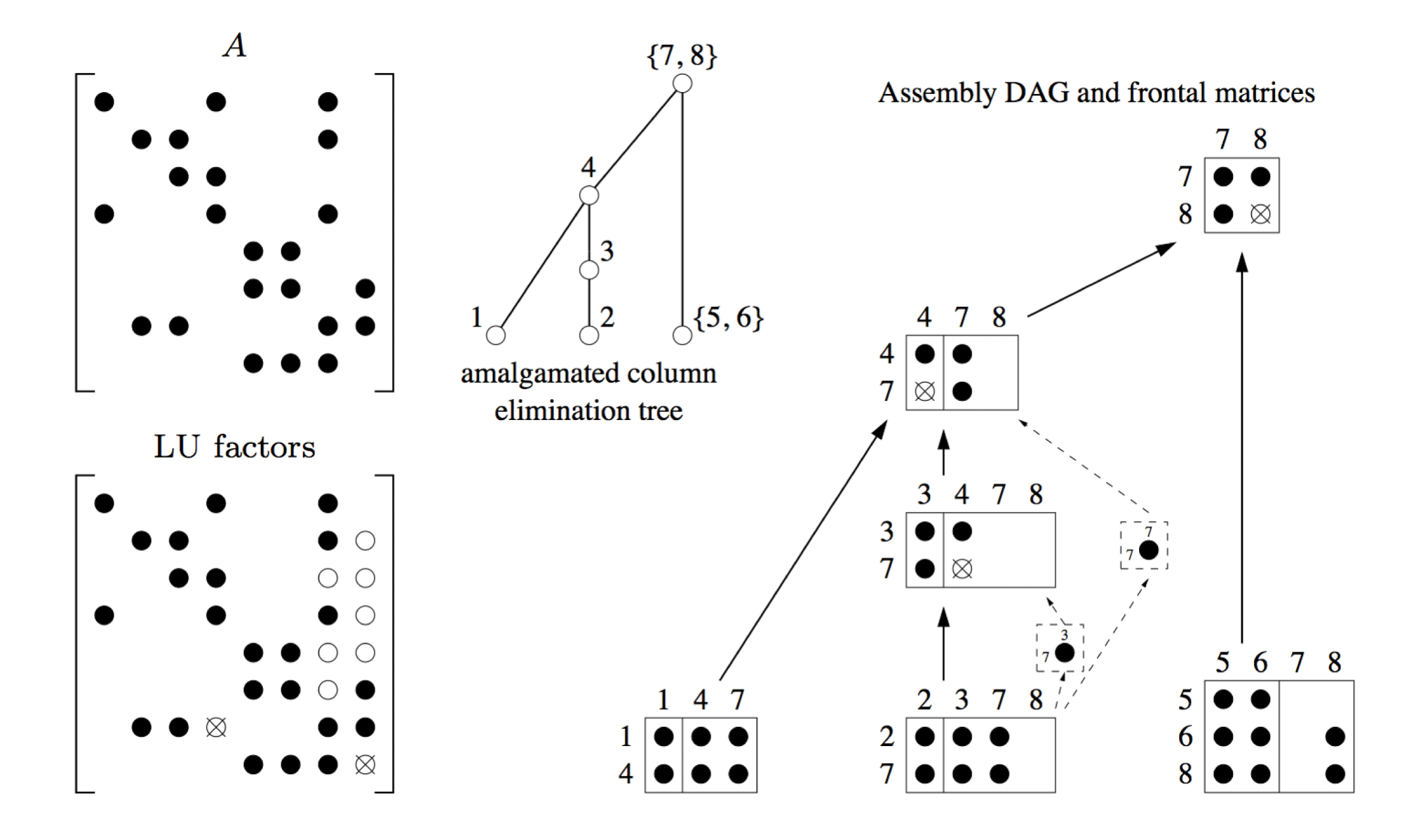
In Figure 11.2 the assembly tree has been expanded to illustrate each frontal matrix. The tree represents the relationship between the frontal matrices, but not the data flow. The assembly of contribution blocks can occur not just between parent and child, but between ancestor and descendant. For example, the contribution to  $a_{77}$ made by frontal matrix 2 could be included in its parent 3, but this would require one additional column to be added to frontal matrix 3. The upper bound of the size of this frontal matrix is 2
 $\times$ 4, but only a 2
 $\times$ 2 frontal matrix needs to be allocated if no partial pivoting occurs. Instead of augmenting frontal matrix 3 to include the
 $a_{77}$ entry, the entry is assembled into the ancestor frontal matrix 4. The data flow between frontal matrices is thus represented by a directed acyclic graph.
One advantage of the right-looking method over left-looking sparse LU factorization is that it can select a sparse pivot row. The left-looking method does not keep track of the non-zero pattern of the  $A^{[k]}$ submatrix, and thus cannot determine the number of non-zeros in its pivot rows. The disadvantage of the right-looking method is that it is significantly more difficult to implement.
The first unsymmetric-pattern multifrontal method (UMFPACK) was by Davis and Duff (Reference Davis and Duff1997). The method keeps track of approximate degrees of the rows and columns of the active submatrix, a symmetric variant of which was later incorporated into the AMD minimum degree ordering algorithm (Amestoy et al. Reference Amestoy, Davis and Duff1996a, Amestoy, Davis and Duff Reference Amestoy, Davis and Duff2004a). The active submatrix is represented as a set of rectangular submatrices (the unassembled contribution blocks of factorized frontal matrices), and the original entries of  $A$ that have yet to be assembled into a frontal matrix. Each row and column consists of two lists: original entries of
 $A$, and a list of contribution blocks that contain contributions to that row or column. The approximate degrees are updated after a frontal matrix is factorized by scanning these lists twice. The first scan provides the set differences. For example, suppose a prior contribution block is 10 by 15, and it appears in three rows of the contribution block
 $C$ of the current frontal matrix. This is found by scanning all the row lists of
 $C$. There are thus seven rows in the set difference. In the second scan, this set difference is used for computing the approximate column degrees. If this contribution block
 $C$ appears in a column list, then it contributes 7 to the approximate degree of that column.
Although its factorization can be viewed as a DAG, this first version of UMFPACK did not actually explicitly create the assembly DAG. Hadfield and Davis (Reference Hadfield and Davis1994, Reference Hadfield and Davis1995) created a parallel version of UMFPACK that introduced and explicitly constructs the assembly DAG. The method relies on the set of frontal matrices constructed by a prior symbolic and numeric factorization, to factorize a sequence of matrices with identical pattern. The DAG is factorized in parallel on a distributed-memory computer. Numerical considerations for subsequent matrices may require pivoting, which is handled by delaying failed pivots to a subsequent frontal matrix. Unlike the symmetric-pattern multifrontal method, the immediate parent may not be suitable to recover from this pivot failure. Instead, the pivot can be accommodated by the first LU parent in the DAG. This is the first ancestor whose row and column non-zero pattern is a superset of the frontal matrix with the failed pivot. This pattern inclusion occurs if there is both an L-path and a U-path from the descendant to the LU-parent ancestor. An L-path is a path in the DAG consisting only of edges from the  $L$ factor, and a U-path consists of edges only in
 $U$.
The sparse multifrontal QR factorization method discussed in the next section (Section 11.5) can also provide a framework for sparse LU factorization, as shown by Raghavan (Reference Raghavan1995). The rectangular frontal matrices for QR factorization of  $A$ can be directly used for the LU factorization of the same matrix. Arbitrary numerical pivoting with row interchanges can be accommodated without changing the frontal matrices found in the symbolic QR pre-ordering and analysis. Raghavan (Reference Raghavan1995) used this approach in a parallel distributed algorithm that can compute either the QR or LU factorization. The method is a multifrontal adaptation of George and Ng’s (Reference George and Ng1990) method for LU factorization, which introduced the QR upper bound for LU factorization.
Davis and Duff (Reference Davis and Duff1999) extended the method by incorporating a technique used to reduce data movement in the frontal method. The frontal matrix currently being factorized acts like a queue. As pivot rows and columns are factorized, their updates are applied to the contribution block and then removed and placed in the permanent data structure for  $L$ and
 $U$. This frees up space for new rows and columns. The factorization continues in this manner until the next frontal matrix would be too large or too different in structure to accommodate the new rows and columns, at which point the contribution block is updated and placed on the contribution block stack. In this manner, the factorization of a parent frontal matrix can be done in the space of the oldest child, thus reducing data movement and memory usage. In the extreme case, if UMFPACK is given a banded matrix that is all non-zero within the band, and assuming no pivoting, then only a single frontal matrix is allocated for the entire factorization, and no contribution block is ever placed on the contribution block stack.
This first version of UMFPACK performed all of its fill-reducing ordering during factorization. Davis (Reference Davis2004a, Reference Davis2004b) then incorporated a symbolic pre-ordering and analysis, using the COLAMD fill-reducing ordering. The frontal matrices are now known prior to factorization. The upper bound on their sizes is found by a symbolic QR analysis, assuming worst-case numerical pivoting, but this bound might not be reached during numerical factorization. A frontal matrix is first allocated space less than this upper bound, to save space, and the space is increased as needed. Because UMFPACK is a right-looking method, and because it maintains the row and column (approximate) degrees, it is still able to search for sparse pivot rows and columns. Thus, the column pre-ordering can be modified during factorization to reduce fill-in. Column pivoting is restricted to within the pivotal column candidates in any one frontal matrix, however, so that the pre-analysis is not broken.
MATLAB makes use of the unsymmetric-pattern multifrontal method (UMFPACK) in  when A is sparse and either unsymmetric, or symmetric but not positive definite. It is also used in [L,U,P,Q]=lu(A). For the [L,U,P]=lu(A) syntax when A is sparse, MATLAB uses GPLU, a left-looking sparse LU factorization (Gilbert and Peierls Reference Gilbert and Peierls1988), discussed in Section 6.2.
Amestoy and Puglisi (Reference Amestoy and Puglisi2002) introduced an unsymmetric version of the multifrontal method that is intermediate between the unsymmetric-pattern multifrontal method (UMFPACK) and the symmetric-pattern multifrontal method (Section 11.1). Like UMFPACK, their frontal matrices can be either square or rectangular. Unlike UMFPACK, they rely on the assembly tree rather than a DAG. The assembly tree is the same as that used for the symmetric-pattern multifrontal method, so that all the contributions of a child go directly to its single parent. However, rectangular frontal matrices are exploited, where the parent’s column pattern is the union of the column patterns of its children, and (separately) the same for its rows. This change has the effect of dropping fully zero rows and/or columns from the square frontal matrices that arise in the symmetric-pattern multifrontal method when the latter is employed on the symmetrized non-zero pattern  $A+A^{T}$ of an unsymmetric matrix
 $A$.
Gupta (Reference Gupta2002a, Reference Gupta2002b) presents two assembly DAGs for the unsymmetric-pattern multifrontal method that can be constructed prior to symbolic factorization. The first one is minimal, and does not allow for partial pivoting during numerical factorization. The second one adds extra edges to accommodate such pivoting. These two DAGs are incorporated into the WSMP package, which includes an implementation of the unsymmetric-pattern multifrontal method. Since the DAGs are known prior to numerical factorization, WSMP can factorize the matrix in parallel on a shared-memory computer. Gupta (Reference Gupta2007) extends this method to a distributed-memory algorithm.
The assembly DAG for the unsymmetric-pattern multifrontal method can be cumbersome, with many more edges than the assembly tree of the symmetric-pattern multifrontal method. Eisenstat and Liu (Reference Eisenstat and Liu2005b) explore the use of a tree instead, to model the assembly of updates from contribution blocks to their ancestors. In this modified tree, the parent of a node is the first node for which there is both an L-path and U-path from child to parent. The assembly DAG adds extra edges to this tree. A bordered-block triangular structure is imposed on the factorization, and then structure is relied on to prune the assembly DAG.
Pothen and Toledo (Reference Pothen, Toledo, Mehta and Sahni2004) survey the use of symbolic structures (trees, DAGs, and graphs) for representing and predicting fill-in, and for the data flow in multifrontal methods. They include a discussion of these symbolic structures for the unsymmetric-pattern multifrontal method.
Avron, Shklarski and Toledo (Reference Avron, Shklarski and Toledo2008) present a shared-memory parallel implementation of the method used in UMFPACK, with a symbolic analysis phase based on the QR and allowing for regular partial pivoting. Unlike UMFPACK, they do not allow for column pivoting during numerical factorization. This algorithmic choice simplifies the method and allows for a better parallel implementation.
11.5 Multifrontal QR factorization
A solution method for sparse linear least-squares systems,
 $$\begin{eqnarray}\min _{x}\Vert Ax-b\Vert _{2},\end{eqnarray}$$
is to solve the augmented system
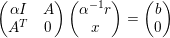 $$\begin{eqnarray}\left(\begin{array}{@{}cc@{}}{\it\alpha}I & A\\ A^{T} & 0\end{array}\right)\left(\begin{array}{@{}c@{}}{\it\alpha}^{-1}r\\ x\end{array}\right)=\left(\begin{array}{@{}c@{}}b\\ 0\end{array}\right)\end{eqnarray}$$
via a sparse Cholesky factorization. The drawback of this approach, however, is that its accuracy depends on the parameter  ${\it\alpha}$, whose optimal value is only approximated through heuristics. QR factorization is an effective alternative. Non-multifrontal sparse QR methods are discussed in Section 7; here we present the multifrontal QR method.
The formulation of the elimination tree for the QR factorization relies on the observation by George and Heath (Reference George and Heath1980) of the strong connection between the QR factor  $R$ and the Cholesky factor of
 $A^{T}A$, via the equality
 $$\begin{eqnarray}A^{T}A=R^{T}(Q^{T}Q)R=R^{T}R.\end{eqnarray}$$
If  $A$ has the strong-Hall property, then the non-zero pattern of the QR factor
 $R$ is the same as the pattern of the Cholesky factorization of
 $A^{T}A$. Otherwise, the pattern of the Cholesky factor of
 $A^{T}A$ is an upper bound, and sometimes it can be quite loose. In this case, however,
 $A$ can be permuted into block upper triangular form (discussed in Section 8.7), and then each diagonal block is a submatrix that is strong-Hall. Many QR factorization methods thus rely on a permutation to block triangular form.
The row-merge tree proposed by Liu (Reference Liu1986c) allows the derivation of the elimination tree of  $A^{T}A$ without ever building this matrix explicitly.
Matstoms (Reference Matstoms1994) proposes a derivation of the multifrontal method for the QR factorization of sparse matrices. He explains the significance of the multifrontal concepts in the context of QR factorization, such as the front, fully summed variables and Schur complement, assembly and factorization operations. He also presents the use of supernodes for efficiency considerations and presents a node amalgamation algorithm to that effect. He then derives a multifrontal QR algorithm on the supernode elimination tree. He finally compares the accuracy and efficiency of the augmented systems, normal equations and multifrontal QR methods.
Matstoms (Reference Matstoms1995) extends his work by discussing a parallel multifrontal QR method on shared-memory environments, with a special emphasis on the memory allocation and deallocation mechanisms. The multifrontal algorithm he uses relies on a hybrid parallelism strategy which consists in switching from the use of tree parallelism, at the bottom of the tree, to the use of node parallelism, at the top of the tree. Fronts of different sizes are then allocated and deallocated in an irregular order. In order to avoid costly memory fragmentation, he proposes a dynamic memory allocation and deallocation mechanism, based on a buddy system using blocks whose sizes are Fibonacci numbers, similar to that proposed by Duff (Reference Duff1989b) and used by Amestoy and Duff (Reference Amestoy and Duff1993), which is based on  $2^{i}$ blocks. He also shows the importance to memory usage of allocating frontal matrices as late as possible.
Raghavan (Reference Raghavan1995) presents a unified distributed-memory multifrontal approach for both LU and QR. She parallelizes both analysis and factorization phases and uses a parallel extension of the Cartesian nested dissection ordering.
Amestoy, Duff and Puglisi (Reference Amestoy, Duff and Puglisi1996b) present a parallel multifrontal QR method (MA49) for a shared-memory context. A specific characteristic of the multifrontal QR method is that a row in the contribution block of a child front is not present in any other child. This offers a degree of freedom on eliminating it either in the parent, as in other multifrontal methods, or in the child. Amestoy et al. study three different front factorization strategies, ranging from standard partial front factorization to full factorization of the whole front (including the contribution block), together with their efficiency and impact on the reduction in the transient fill-in and the storage of the Householder vectors. They also show the impact of relaxed node amalgamation and use of Level 3 BLAS on improving the efficiency of the factorization and solve phases.
Sun (Reference Sun1996) proposes a distributed-memory multifrontal QR method. He uses the proportional mapping by Pothen and Sun (Reference Pothen and Sun1993) to map the supernodal elimination tree on the processors. His parallel factorization kernel merges two upper triangular matrices, through Givens rotations, to obtain another upper triangular matrix. Moreover, he relies on a one-dimensional block cyclic distribution of the frontal matrices on the processors. He proposes the equal-row and equal-volume partitioning scheme for partitioning the two upper triangular matrices, the latter partitioning being intended to fix the load imbalance of the former, which is due to the trapezoidal shape of the matrices. Furthermore, he shows that a column-oriented layout is more efficient than a row-oriented one, for reasonably large numbers of rows. He also proposes a parallel assembly algorithm.
Lu and Barlow (Reference Lu and Barlow1996) propose a multifrontal QR method based on Householder transformations. Their idea is to store the Householder matrices of each front instead of computing and storing the whole Q matrix directly, which would include an excessive amount of fill-in. This implicit multifrontal way of storing the Q matrix allows for the computation of  $Q^{T}b$ for the solve phase. Moreover, instead of forming the frontal Householder matrices explicitly, they rely on an implicit lower trapezoidal representation in which each column is a Householder vector of the front. This YTY (or storage-efficient WY) representation allows them to use efficient Level 2 BLAS in the solve phase. They develop upper bounds on the storage requirement of this storage scheme in the multifrontal QR method for a model problem and for the
 $\sqrt{n}$-separator problem. They also show that this representation requires less storage than the WY representation, with a penalty on efficiency.
Pierce and Lewis (Reference Pierce and Lewis1997) introduce an approximate rank-revealing multifrontal QR method (RRQR). It aims at expressing the factors of the QR factorization as
 $$\begin{eqnarray}\left(\begin{array}{@{}cc@{}}R & S\\ 0 & T\end{array}\right)\!,\end{eqnarray}$$
where  $[S~T]^{T}$ corresponds to the rank-deficient columns. Their method consists of two phases. In the first phase, the multifrontal QR factorization is applied. Given the largest Euclidean norm of a column of A, as an approximation to the largest singular value of A, and, given the approximated smallest singular value of the submatrix related to the subtree rooted at the current front, which is obtained through the SPICE algorithm of Bischof et al. (Reference Bischof, Lewis and Pierce1990), the ratio of these two values is compared to a threshold value in order to determine the rank-deficiency of the current front. During the factorization of such fronts, rank-deficient fully summed columns are detected and prohibited from elimination, in the current front and any ancestor in the tree. These columns then correspond to the
 $[S~T]^{T}$ matrix. Pierce and Lewis show that the bound on the Frobenius norm of
 $T$ obtained there is
 $O(2k+1)$, where
 $k$ is the order of
 $T$. The heart of their method is the second phase. Whenever
 $$\begin{eqnarray}\Vert T\Vert _{F}>\sqrt{(nk)(k+1)},\end{eqnarray}$$
a dense RRQR factorization is applied to T, which orders the columns of the reduced matrix by norm. A first set of columns of this reduced matrix may then be included back in  $R$, and the other set, the largest trailing principal submatrix, then has a Frobenius norm less than
 $((nk)(k+1))^{1/2}$.
Davis (Reference Davis2011a) provides an implementation of the multifrontal QR factorization for the sparse QR factorization method that is built into MATLAB, called SuiteSparseQR. It is based on the method of Amestoy et al. (Reference Amestoy, Duff and Puglisi1996b), and also extends that method by adapting Heath’s (Reference Heath1982) method for handling rank-deficient matrices. It exploits shared-memory parallelism via Intel’s Threaded Building Blocks library. It does not exploit the block triangular form in its fullest extent, because that form is not compatible with its method for handling rank-deficiency. However, it does exploit singletons, which are 1  $\times$ 1 blocks in the block triangular form. These arise very frequently in problems from a wide range of applications. SuiteSparseQR is used for
 in MATLAB when A is rectangular, and for qr(A) when A is sparse. The GPU-accelerated version of SuiteSparseQR is discussed in Section 12.3.
Edlund (Reference Edlund2002) presents a multifrontal LQ factorization. He presents the design of an updating and downdating algorithm together with the dynamic representation of the  $L$ matrix that he uses. This representation is more suitable than the usual static representations for handling the dynamic transformations of its sparsity pattern induced by the updating and downdating. He also presents the technique that he uses to permute reducible matrix to block triangular form, with irreducible square diagonal blocks. He introduces a variant of the approximate minimum degree similar to the COLAMD ordering by Davis et al. (Reference Davis, Gilbert, Larimore and Ng2004a). As he is interested only in the structure of
 $L$, his algorithm only considers the structure of
 $A$ instead of the structure of
 $AA^{T}$. The symbolic factorization algorithms he presents is derived from this variant to build the elimination tree. He shows that the use of element counters during this phase allows one to find a correct prediction of the fill-in after the block triangularization. Finally, he presents his multifrontal approach, which is based on that of Matstoms (Reference Matstoms1994).
Buttari (Reference Buttari2013) proposes a multifrontal QR method for shared-memory environments. His approach is based on the observation that the traditional combined use of node and tree parallelism is restricted by the coarse-grained granularity of parallelism as defined by the elimination tree. He thus proposes a fine-grained partitioning of data where the expression of the dependencies on tree parallelism, expressed by the elimination tree, is combined with the dependencies on node parallelism, expressed by the dense factorization dataflow within each front, through the use of a DAG. This model allows a smoother expression of the dependencies between computations, and removes the restrictive synchronization between the activation of a parent front and the completion of its children. Buttari then proposes a dynamic scheduling of the computational tasks. He relies on dataflow parallel programming model where the schedulable tasks are broken down to sequential tasks and where sequential BLAS is used instead of multithreaded BLAS. He pays a particular attention to data locality and minimization of memory bank conflicts between different processors. The dataflow model he chooses allows a natural extension of the solver to the use of runtime systems by Agullo, Buttari, Guermouche and Lopez (Reference Agullo, Buttari, Guermouche and Lopez2014) for the scheduling of the tasks. The method of Agullo et al. (Reference Agullo, Buttari, Guermouche and Lopez2014) can exploit heterogeneous systems with GPUs, and is discussed in Section 12.3.
12 Other topics
In this section we consider several topics that have been postponed until now, primarily because they rely on all of the prior material that has been discussed so far. Section 12.1 presents the update/downdate problem, in which a matrix factorization is to be recomputed after the matrix  $A$ undergoes a low-rank change. It can be computed faster than a forward/backsolve to solve
 $Ax=b$ with the resulting factors. Section 12.2 presents a survey of parallel methods for the forward/backward triangular solve. Algorithms for sparse direct methods on GPUs are the topic of Section 12.3 for both supernodal and multifrontal methods. Section 12.4 presents the use of low-rank approximations in sparse direct methods. The off-diagonal blocks of a matrix factorization, whether sparse or dense, can have low numerical rank. This property can be exploited to reduce both time and memory requirements to compute the factorization, while at same time maintaining the same level of accuracy that sparse direct methods are known for.
12.1 Updating/downdating a factorization
Once a matrix  $A$ is factorized, some applications require the solution of a closely related matrix,
 $\overline{A}=A\pm W$, where the matrix
 $W$ has low rank. Computing the factorization of the matrix
 $\overline{A}$ by modifying the existing factorization of
 $A$ can often be done much faster than factorizing
 $\overline{A}$ from scratch, both in practice and in an asymptotic, big-
 $O$ sense. Constructing the factorization of
 $\overline{A}=A+W$ is referred to as an update, and factorizing
 $\overline{A}=A-W$ is a downdate. The problem arises in many applications. For example, when the basis set changes in optimization, columns of
 $A$ come and go. In the simultaneous localization and mapping problem (SLAM) in robotics, new observations are taken, which introduce new rows in a least-squares problem. In the finite element method, cracks can propagate through a physical structure, and as the crack propagates, only a small local refinement is required to solve the new problem. In the circuit simulation domain, short-circuit analysis requires the solution of a linear system after successive pairs of contacts are shorted together, resulting in a very small change to a matrix that was already just factorized.
Constructing the updated/downdated factorization is much faster than computing the original factorization. The total time is often less than the triangular solves (forward/backsolve) with the resulting factors. That is, it can take less time to modify the factorization than it takes to solve the resulting system with the factorized matrix.
12.1.1 Modifying an LU factorization
The very first sparse update/downdate methods were motivated by the simplex method in linear programming. The goal is to find the optimal solution to an underdetermined system of equations  $Ax=b$, where
 $A$ has more columns than rows. The simplex method constructs a sequence of basis matrices, which are composed of a subset of the columns of
 $A$. As the method progresses, columns come and go in the basis, resulting in an update and downdate, respectively. Since
 $A$ is unsymmetric, an LU factorization is used, along with methods to update/downdate the LU factors when columns come and go.
The first method appeared in a 1970 IBM technical report by Brayton et al., which formed the basis of the method of Tomlin (Reference Tomlin, Rose and Willoughby1972) and Forrest and Tomlin (Reference Forrest and Tomlin1972). To modify a column, the method deletes a column  $k$ of
 $U$ and shifts the remaining columns to the left. The incoming column is added at the end, resulting in a sparse upper Hessenberg matrix. Next, the
 $k$ row is moved to the end of the matrix, resulting in a matrix that is upper triangular except for the last row. Pairwise (non-orthogonal) eliminations between rows
 $k$ and
 $n$, then
 $k+1$ and
 $n$, and so on, reduce the matrix back to upper triangular form. Pivots are taken from the diagonal, and thus fill-in is limited to the last row and column in the new factorization. No numerical pivoting is performed, and thus the method can be unstable if the diagonal entries are small relative to the entries in the last row
 $n$.
Reid (Reference Reid1982) presents a similar method, a sparse variant of Bartel and Golub’s method. The new column is placed not at the end, but in the column  $r$ if its last non-zero entry resides in row
 $r$. It does not permute the row
 $k$ to the end, but operates on the upper Hessenberg matrix instead, where only rows
 $k$ to
 $r$ are upper Hessenberg and the remainder starts as already upper triangular. The method uses pairwise pivoting between rows
 $k$ and
 $k+1$, then
 $k+1$ and
 $k+2$, and so on, to reduce the matrix back to upper triangular form. Pivots can thus be chosen via relaxed pairwise pivoting, where the sparser row of the two is selected if its pivotal leftmost non-zero entry is large enough. Row and column singletons within the submatrix
 $A(k:r,k:r)$ are exploited to reduce the size of the upper Hessenberg submatrix via row and column swaps. The method reduces fill-in compared to Forrest and Tomlin’s method, and also improves stability.
Reid’s (Reference Reid1982) method is complex, and Suhl and Suhl (Reference Suhl and Suhl1990, Reference Suhl and Suhl1993) consider a simpler variant based on a modification of Tomlin’s approach. Starting with the upper Hessenberg submatrix  $A(k:r,k:r)$ of Reid’s method, they reduce the matrix to upper triangular form by relying on diagonal pivots, just like Forrest and Tomlin. Note that the term ‘fast’ in the title of Suhl and Suhl’s paper is meant in a practical sense, not in a theoretical, asymptotic sense. In particular, no LU update/downdate method takes time proportional to the number of entries in
 $L$ and
 $U$ that need to be modified, which is a lower asymptotic bound on any update/downdate method. This bound is reached for updating/downdating a Cholesky factorization, as discussed below.
12.1.2 Modifying a Cholesky factorization
Given the sparse Cholesky factorization  $LL^{T}=A$, computing the factorization
 $\overline{LL}^{T}=A+WW^{T}$, where
 $W$ is
 $n\times k$ with
 $k\ll n$, is a rank-
 $k$ update, and computing
 $\overline{LL}^{T}=A-WW^{T}$ is a rank-
 $k$ downdate.
Law (Reference Law1985) and Law and Fenves (Reference Law and Fenves1986) present a method that updates the numerical values of  $L$ but not its non-zero pattern after a rank-
 $k$ change. The first pass takes
 $O(n)$ time to determine which columns need to change, and the second pass uses partial refactorization to compute those columns. The time taken is proportional to the sum of squares of the column counts of the columns that change. That is, if
 ${\mathcal{X}}$ denotes the columns of
 $L$ that change, the method takes
 $O(n+\sum _{j\in {\mathcal{X}}}|{\mathcal{L}}_{j}|^{2})$ time. Law (Reference Law1989) extends this method to allow for a change in the non-zero pattern of
 $L$, and shows that the columns that change are governed by paths in the elimination tree. The method updates the tree as the pattern of
 $L$ changes.
Davis and Hager (Reference Davis and Hager1999) present the first asymptotically optimal rank-1 update/downdate method, taking  $O(\sum _{j\in {\mathcal{X}}}|{\mathcal{L}}_{j}|)$ time. They show that a rank-1 update modifies all columns along the path from
 $p$ to the root of the elimination tree, where
 $p$ is the first non-zero in the column vector
 $w$. If the pattern changes, the path in the new tree is followed. The entire algorithm (finding the path, modifying both the pattern and values of
 $L$, and modifying the tree) takes time proportional to the number of entries in
 $L$ that change. A rank-1 update is shown in Figure 12.1. The key observation is that the columns that change correspond to the non-zero pattern of the lower triangular system
 $Lx=w$, with a sparse right-hand side
 $w$ (Section 3.2).
Rank-1 update  $A+ww^{T}$ that changes the pattern of
 $L$. The old elimination tree is
 ${\mathcal{T}}$ and the new tree is
 $\overline{{\mathcal{T}}}$. Non-zeros that do not change are shown as solid circles; non-zeros that change are shown as circled x’s. The columns that are modified (4, 6, 7, and 8) become a path in
 $\overline{{\mathcal{T}}}$ (Davis Reference Davis2006).
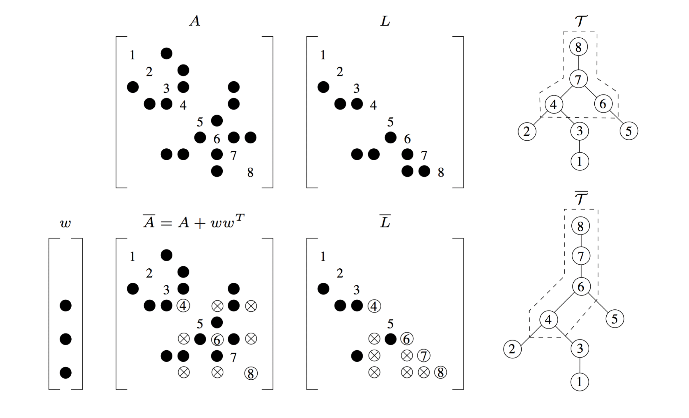
Davis and Hager (Reference Davis and Hager2001) extend this to an asymptotically optimal rank- $k$ update, which modifies a set of
 $k$ paths in the tree. They also show how to add/delete rows and columns of the matrix (Davis and Hager Reference Davis and Hager2005), and how to exploit supernodes for increased performance (Davis and Hager Reference Davis and Hager2009). Supernodes can both split or merge during an update or downdate. The methods are implemented in CHOLMOD (Chen et al. Reference Chen, Davis, Hager and Rajamanickam2008). A simpler rank-1 update/downdate that does not change the pattern of
 $L$ appears in CSparse (Davis Reference Davis2006).
Downdating  $A-ww^{T}$ can lead to symbolic cancellation of entries in
 $L$; Davis and Hager track this by replacing each set
 ${\mathcal{L}}_{j}$ with a multiset that keeps track of the multiplicity of each entry. When the multiplicity drops to zero, the entry can be removed. Keeping this doubles the integer space required for
 $L$, and thus CHOLMOD does not include the multiplicities. Dropping these entries is optional, and to do so requires a reconstruction of the symbolic factorization, taking time
 $O(|L|)$.
12.1.3 Modifying a QR factorization
Since the Cholesky factorization of  $A^{T}A$ results in the QR factor
 $R$ (assuming
 $A$ is strong-Hall), the update/downdate of a QR factorization is very similar to the Cholesky update/downdate. A new row
 $w$ appended to
 $A$ has the same structure of computation as a rank-1 Cholesky update
 $A+ww^{T}$.
Björck (Reference Björck1988) shows that adding a row to  $R$ can be done via a series of Givens rotations with the new row
 $w$ and rows of the existing
 $R$. Exploiting the assumption that the non-zero patterns of the rows to be added to
 $A$ are known in advance allows for a static non-zero pattern of
 $R$ and a static data structure to hold it. This assumption holds for active set methods in optimization, and many other applications.
Edlund (Reference Edlund2002) extends Davis and Hager’s method for a multifrontal LQ factorization (an LQ factorization is essentially the QR factorization of  $A^{T}$). He considers the important case when
 $A$ is not strong-Hall, an issue that does not arise in the Cholesky update/downdate problem.
The GPU is well-suited to a multifrontal or supernodal factorization since those methods rely on the regular computations within dense submatrices. However, GPUs can also accelerate the left-looking sparse LU factorization without the need to rely on dense matrix computations. Chen, Ren, Wang and Yang (Reference Chen, Ren, Wang and Yang2015) extend their NICSLU method to the GPU. It differs from their prior method for a multicore CPU (Chen et al. Reference Chen, Wang and Yang2013), in that it assumes no numerical pivoting is required. This assumption works well for their target circuit simulation application, where a sequence of matrices are to be factorized. Each task in NICSLU executes on a single warp on the GPU. He, Tan, Wang and Shi (Reference He, Tan, Wang and Shi2015) present a right-looking variant for the GPU. Like the first phase of NICSLU, their method operates on the column elimination tree level by level. All the columns at a given level are first scaled by the diagonal of  $U$, obtaining the corresponding columns of
 $L$. Next, all warps cooperate to update the remainder of the matrix, to the right. Each warp updates an independent subset of these target columns from the columns of
 $L$ computed in this level.
12.2 Parallel triangular solve
Solving a sparse linear system requires a fill-reducing ordering, a symbolic analysis (or at least most methods do), a numerical factorization, and finally, the solution of the triangular system or systems. Basic methods for solving a triangular system with both a dense and sparse right-hand side have already been discussed in Section 3. We now consider how to do this step in parallel. Rather than including this discussion in Section 3, we present it now because many of the methods depend on the supernodal or multifrontal factorizations presented in Sections 9 and 11.
Solving the lower triangular system  $Lx=b$ is difficult to parallelize because the computational complexity (ratio of flops over bytes, or over
 $O(|L|)$) is so low. If
 $b$ is a vector, the ratio is just 2, regardless of
 $L$. The numeric factorization has a much higher computational complexity, namely
 $O(\sum |{\mathcal{L}}_{j}|^{2}/\sum |{\mathcal{L}}_{j}|)$, which in practice can be as high as
 $O(n^{2/3})$ for a matrix arising from a three-dimensional mesh. As a result, often the goal of a parallel triangular solve for a distributed-memory solver is to leave the matrix
 $L$ distributed across the processor memories that contain it, and not to experience a parallel slowdown.
The method used can depend on whether  $L$ arises from a Cholesky or QR factorization (in which case the elimination tree describes the parallelism), or if
 $L$ arises from LU factorization, in which case
 $L$ can be arbitrary. In the former case, the special structure of
 $L$ allows for more efficient algorithms.
Two classes of methods are considered below. The first methods are based on the triangular solve discussed in Section 3, with both dense (Section 3.1) and sparse (Section 3.2) right-hand sides. The second class of methods is based on computing explicit inverses of submatrices of  $L$.
12.2.1 Methods based on the conventional triangular solve
Wing and Huang (Reference Wing and Huang1980) consider a fine-grained model of computation, where each division or multiply-add becomes its own task, and give a method for constructing a task schedule on a theoretical machine model. Consider the problem of solving  $Lx=b$ where
 $L$ is lower triangular. The non-zero entry
 $l_{ij}$ means that
 $x_{j}$ must be computed prior to the update
 $x_{i}=x_{i}-l_{ij}x_{j}$, just as discussed in the topological ordering for the sparse triangular solve in Section 3.2. This gives a task dependency graph, which is directed acyclic (a DAG), as shown in Figure 3.2, with an edge
 $(j,i)$ for each non-zero
 $l_{ij}$. Wing and Huang (Reference Wing and Huang1980) discuss a level scheduling method, via a breadth-first traversal where the first level consists of all nodes
 $j$ for which the corresponding row
 $j$ is all zero except for the diagonal (nodes with no incoming edges). When solving
 $Ux=b$ the edges go in the opposite direction, from high numbered nodes to lower numbered nodes. Ho and Lee (Reference Ho and Lee1990) propose a modification to this method that changes with additional eliminations that increases the non-zeros in
 $L$, but also increases the available parallelism.
The first practical algorithm and software for solving this problem in parallel was by Arnold, Parr and Dewe (Reference Arnold, Parr and Dewe1983). They rely on semaphores in a shared-memory computer to ensure that two updates ( $x_{i}=x_{i}-l_{i,j1}x_{j1}$ and
 $x_{i}=x_{i}-l_{i,j2}x_{j2}$) to the same
 $x_{i}$ do not conflict. The updates from
 $x_{j}$ can start as soon as all updates from incoming incident nodes are completed. Each task is the same as that of Wing and Huang (Reference Wing and Huang1980).
George et al. (Reference George, Heath, Liu and Ng1986a) use a medium-grained computation where each task corresponds to a column of  $L$. The backsolve (
 $L^{T}x=b$) is thus done by rows, and task (row)
 $j$ waits for each
 $k$ to be completed first, for each non-zero
 $l_{kj}$. No critical section is required. In the forward solve, multiple tasks can update the same entries, so synchronization is used just as in Arnold et al.’s (Reference Arnold, Parr and Dewe1983) method, with a critical section for each entry in
 $x$. They extend their method to a distributed-memory computer where the columns of
 $L$ are distributed across the processors (George et al. Reference George, Heath, Liu and Ng1989a). Kumar, Kumar and Basu (Reference Kumar, Kumar and Basu1993) extend this method by exploiting the dependency structure with the elimination tree, rather than using the larger structure of the graph of
 $L$.
Operating on submatrices rather than individual entries (Wing and Huang Reference Wing and Huang1980) or rows or columns (George et al. Reference George, Heath, Liu and Ng1986a) can improve performance because it reduces the scheduling and synchronization overhead. Saltz (Reference Saltz1990) demonstrates this in his scheduling method which reduces the size of the DAG of a general matrix  $L$ by merging together sets of nodes that correspond to subpaths in the DAG. When
 $L$ arises from a supernodal Cholesky factorization, the supernodal structure provides a natural partition for improving performance (Rothberg Reference Rothberg1995), by allowing each processor to use Level 2 BLAS and by reducing parallel scheduling overhead. Each diagonal block of a supernode is a dense lower triangular matrix, allowing use of Level 2 BLAS. The method also extends to the triangular solves from a multifrontal QR factorization (Sun Reference Sun1997). Mayer (Reference Mayer2009) introduces an alternative two-dimensional mapping of the parallel computation, where each block anti-diagonal can be computed in parallel.
Totoni, Heath and Kale (Reference Totoni, Heath and Kale2014) also distribute larger submatrices to each processor. They pipeline the computation between dependent processors to send more critical messages early, which correspond to data dependencies on the critical path. The matrix is distributed mostly by blocks of columns, except that dense submatrices are also distributed to increase parallelism. The method scales up to 64 cores for many matrices, and beyond that for a few. It can obtain superlinear speedup because of local cache effects.
All of the methods described so far assume that the matrix  $L$ resides in the single shared-memory space of a shared-memory computer, or that it is distributed across the memory spaces of a distributed-memory computer. In out-of-core methods, the matrix
 $L$ is too large for this, and must be held in disk, with only parts of
 $L$ held in main memory at any one time. Amestoy, Duff, Guermouche and Slavova (Reference Amestoy, Duff, Guermouche and Slavova2010) consider the out-of-core, distributed-memory solve phase for a parallel multifrontal method. The parallelism is governed by the elimination tree (the assembly tree to be precise) since the factors are assumed to have a symmetric structure.
12.2.2 Methods based on explicit inversion of submatrices
Matrix multiplication provides more scope for parallelism than a triangular solve. Solving a linear system by multiplying by the inverse of an entire non-triangular sparse matrix is not a good idea since the inverse of a strong-Hall matrix is completely non-zero. However, a triangular matrix is not strong-Hall. Anderson and Saad (Reference Anderson and Saad1989) exploit this fact by explicitly inverting small diagonal submatrices of  $L$. Suppose the following
 $L_{11}$ block is small but not a scalar:
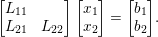 $$\begin{eqnarray}\left[\begin{array}{@{}cc@{}}L_{11} & \\ L_{21} & L_{22}\end{array}\right]\left[\begin{array}{@{}c@{}}x_{1}\\ x_{2}\end{array}\right]=\left[\begin{array}{@{}c@{}}b_{1}\\ b_{2}\end{array}\right]\!.\end{eqnarray}$$
Then  $x$ can be computed with
 $x_{1}=L_{11}^{-1}b_{1}$, followed by the solution to the smaller system
 $L_{22}x_{2}=b_{2}-L_{21}x_{1}$, which can be further subdivided and the same method applied. If
 $L_{11}$ is diagonal, it is easy to invert. In general
 $L_{11}^{-1}$ has more non-zeros than
 $L_{11}$, but it always remains lower triangular. Anderson and Saad (Reference Anderson and Saad1989) consider several methods for solving
 $Lx=b$ in parallel, including one that only inverts diagonal submatrices, and another that requires extra fill-in. In the latter method, they partition
 $L$ into fixed-size diagonal blocks and invert each block. Their method is intended for shared-memory parallel computers; González, Cabaleiro and Pena (Reference González, Cabaleiro and Pena2000) adapt this method for the distributed-memory domain.
Law and Mackay (Reference Law and Mackay1993) rely on inverting dense diagonal submatrices so that no extra fill-in occurs. The partitions are the same as those used by George (Reference George1977a), where the diagonal blocks are dense and the subdiagonal blocks can be represented in an envelope form with no extra fill-in. These partitions are larger than the diagonal blocks of fundamental supernodes.
Alvarado, Yu and Betancourt (Reference Alvarado, Yu and Betancourt1990) go beyond the idea of exploiting inverses of diagonal submatrices to construct a partitioned inverse representation of  $L$. The matrix
 $L$ can be viewed as the product of
 $n$ elementary lower triangular matrices, each of which is diagonal except for a single column. The inverse of each of these matrices is easy to represent with no extra fill-in. This gives a simple partitioned inverse with
 $n$ partitions of a single column each. They show that larger partitions can be formed instead, and when each one is explicitly inverted, no fill-in occurs. Larger partitions can be formed but they result in extra fill-in. Alvarado and Schreiber (Reference Alvarado and Schreiber1993) prove that this method constructs optimal partitions, assuming that each partition consists of adjacent columns of
 $L$ (with no permutations allowed), and also present another method that finds optimal partitions when permutations are allowed. This results in larger partitions, but the method is very costly, taking
 $O(n|L|)$ time in the worst case to find the partitions. Pothen and Alvarado (Reference Pothen and Alvarado1992) cut the time drastically by assuming
 $L$ arises from a Cholesky factorization. They exploit the chordal property of the graph of
 $L+L^{T}$ to find optimal partitions in only
 $O(n)$ time, allowing for a restricted set of permutations. Alvarado, Pothen and Schreiber (Reference Alvarado, Pothen, Schreiber, George, Gilbert and Liu1993) survey all of these variations of the partitioned inverse method.
Peyton, Pothen and Yuan (Reference Peyton, Pothen and Yuan1993) further develop this method by allowing for a wider range of possible permutations. These permutation differ in that they must be applied to  $A$ prior to its Cholesky factorization, but they result in fewer, larger partitions, and thus increase the amount of available parallelism in the triangular solve. Their method takes
 $O(n+|L|)$ time, which is higher than Pothen and Alvarado’s (Reference Pothen and Alvarado1992) method but still very practical. Peyton, Pothen and Yuan (Reference Peyton, Pothen and Yuan1995) present an alternative algorithm for this problem that cuts the time to
 $O(n+q)$, where
 $q$ is size of the clique tree (Section 9.1), which is typically far less than
 $O(|L|)$ in size.
Raghavan (Reference Raghavan1998) takes an alternative approach, which is more closely related to Anderson and Saad’s (Reference Anderson and Saad1989) method. Rather than inverting the entire partition, the inversion is limited to the diagonal blocks of supernodes (which are already dense) that are spread across multiple processors.
12.3 GPU-based methods
Recently, a new kind of computer architecture has begun to have an impact on computational science, and on sparse direct methods in particular. Modern CPU cores rely on complex instruction execution hardware that allows for out-of-order execution and superscalar performance. They require a high clock rate to obtain high performance. The downside to this approach is the power consumption and size of the cores. An alternative approach is to use a large number of simpler processors, and to share the instruction execution unit and/or the memory interconnect. Graphics processing units (GPUs) are on one end of this spectrum, where groups of cores share a single execution unit and an interface to memory. All threads in a group thus execute the same instructions, just on different data. These GPUs are no longer targeted just for graphics processing, but for general computing (examples include GPUs from NVIDIA and AMD). The Intel Xeon Phi takes a different approach, packing many simpler processors on a single chip in a design that trades high clock speed and core complexity for many simpler cores running at a lower clock speed, each with their own instruction fetch/decode/execute unit. The result in both cases is a high-throughput computational engine, at a much lower power consumption. Either of these approaches results in a parallel computational environment with many closely coupled threads.
The architectures work well for regular parallelism, but pose a challenge for sparse direct methods because of the irregular nature of the algorithms. For example, the elimination tree is often unbalanced. Dense submatrices exist in the factors and can be exploited by supernodal, frontal, and multifrontal methods, but they vary greatly in size, even between two nodes at the same level of the elimination tree. Gather/scatter leads to a very irregular memory access.
In the GPU computing model, independent tasks are bundled together in a kernel launch. The GPU has a dozen or so instruction execution units, each of which controls a set of cores (32, say). In NVIDIA terminology, these are called streaming multiprocessors, or SMs. Each SM executes a larger number of threads (a few hundred), called a thread block. The hardware scheduler on the GPU assigns the tasks in a kernel launch to a thread block. At a high-level view, the threads in a thread block can be thought of as working in lock-step. However, they are actually broken into subgroups of threads (called warps). Each warp is executed one at a time on the instruction unit. When the threads in one warp place a request for global memory, the warp is paused and another warp, one whose memory reference is ready, is executed instead. The switch between warps happens in hardware, with no scheduling delay. If the threads in a warp encounter an if-then-else conditional statement, then all threads for which the condition is true are executed, and the rest remain idle, and then the opposite is done for the threads for which the condition is false. In most GPUs, the GPU and CPU memories are distinct, and data must be transferred explicitly between them, although this is changing with some CPU cores containing GPUs on-chip.
Pierce et al. (Reference Pierce, Hung, Liu, Tsai, Wang and Yu2009) off-load large frontal matrices to the GPU in their multifrontal Cholesky factorization method. A frontal matrix is sent to the GPU, factorized, and brought back. Small frontal matrices remain on the CPU. Krawezik and Poole (Reference Krawezik and Poole2009) take a similar approach, except that their method shares the work for large frontal matrices between the CPU and GPU. The factorization of each diagonal block in the frontal matrix is done on the CPU and transferred to the GPU, which is responsible for the subsequent update of the lower-right submatrix, a large dense matrix–matrix multiply. Lucas, Wagenbreth, Davis and Grimes (Reference Lucas, Wagenbreth, Davis and Grimes2010) and George et al. (Reference George, Saxena, Gupta, Singh and Choudhury2011) develop this method further by exploiting the parallelism of the CPU cores of the host. The many smaller frontal matrices at the lower levels of the tree provide ample parallelism for the CPU cores. Towards the root of the tree, where the frontal matrices are larger, the GPU is used. George et al. (Reference George, Saxena, Gupta, Singh and Choudhury2011) also exploit multiple GPUs.
Yu, Wang and Pierce (Reference Yu, Wang and Pierce2011) extend GPU acceleration to the unsymmetric-pattern multifrontal method. They perform the dense matrix updates for a frontal matrix on the GPU. Pivoting, and the dense triangular solves required for computing the pivot row and column, are computed on the CPU. Assembly operations between child and parent frontal matrices are done on the CPU, while updates within large frontal matrices are computed and assembled on the GPU.
The software engineering required to create GPU-accelerated algorithms is a complex task. Lacoste et al. (Reference Lacoste, Ramet, Faverge, Ichitaro and Dongarra2012) alleviate this by relying on runtime scheduling frameworks in their right-looking supernodal factorization (Cholesky,  $\text{LDL}^{\text{T}}$, and LU with static pivoting). Their method can exploit multiple CPUs and multiple GPUs. Large supernodal updates are off-loaded to the GPU.
In all of the multifrontal methods discussed so far, the contribution blocks from child frontal matrices are assembled into their parents on the CPU. Large frontal matrices are transferred to the GPU, factorized there one at a time, and then brought back to the CPU. The GPU factorizes a single frontal matrix at a time. Likewise, in the GPU-accelerated supernodal methods described so far, each GPU works on a single supernodal update at a time.
Rennich, Stosic and Davis (Reference Rennich, Stosic and Davis2014) break this barrier by allowing each GPU to work on many supernodes at the same time. Their method batches together many small dense matrix updates in their supernodal Cholesky factorization. They use this strategy for subtrees that are small enough to fit on the GPU. Once all subtrees are factorized, their method works on the larger supernodes towards the root of the tree, one at a time. The work for large supernodes is split between the CPU and the GPU, with the CPU performing the updates from smaller descendants and the GPU performing the updates for the larger descendants.
Hogg, Ovtchinnikov and Scott (Reference Hogg, Ovtchinnikov and Scott2016) present a GPU-accelerated multifrontal solver for symmetric indefinite matrices, which require pivoting; prior methods did not accommodate any pivoting. They use the GPU to factorize many frontal matrices at the same time. Frontal matrices are assembled on the GPU rather than bringing them back to the CPU for assembly. This allows the GPU to handle small frontal matrices effectively.
Sao, Vuduc and Li (Reference Sao, Vuduc, Li, Silva, Dutra and Santos Costa2014) present a GPU-accelerated algorithm based on SuperLU_DIST, which is a parallel distributed-memory LU factorization based on a right-looking supernodal method. It can exploit multiple CPUs and GPUs. The GPUs are used to accelerate the right-looking Schur complement update, which is the dominant computation. Factorizing the supernodes is left to the CPUs. Small dense matrix updates on the GPU are aggregated into larger updates. Multiple such updates are pipelined with each other and with the transfer of their results back to their corresponding CPU host, which holds the supernodes. The CPU then applies the results of the update to the target supernodes (the scatter step). They extend this work to the Intel Xeon Phi (Sao, Liu, Vuduc and Li Reference Sao, Liu, Vuduc and Li2015). In this method, the work for the Schur complement update for large supernodes is shared between the CPU host and the GPU. Furthermore, the scatter step of assembling the results of the dense submatrix updates back into the target supernodes is done on the GPU.
Yeralan, Davis and Ranka (Reference Yeralan, Davis and Ranka2015) present a multifrontal sparse QR factorization in which all floating-point work is done on the GPU. They break the factorization of each frontal matrix into a set of tiles, and individual SMs operate in parallel on different parts of a frontal matrix. At each kernel launch, the GPU can be factorizing many frontal matrices at various stages of completion, while at the same time assembling contribution blocks of children into their parents. Scheduling occurs at a finer granularity than levels in the elimination tree; the GPU does not have to wait until all frontal matrices in a level of the tree are finished before factorizing the parents of these frontal matrices. Frontal matrices are created, assembled, and factorized on the GPU. The only data transferred to the GPU is the input matrix, and the only data that comes back is the factor  $R$.
Agullo et al. (Reference Agullo, Buttari, Guermouche and Lopez2014) show how a runtime system can be used to effectively implement the multifrontal sparse QR factorization method on a heterogeneous system. Their method relies on both the CPUs and the GPUs to perform the numerical factorization. A runtime system provides a mechanism for scheduling the tasks in a parallel algorithm based on the task dependency DAG of the algorithm. It ensures the data dependencies are satisfied. The runtime system may run any given task on either a multicore CPU or on a GPU, which raises a potential problem: the data required by the GPU may reside on the CPU, and where each task is executed is not known a priori. To resolve this, they rely on a new scheduling mechanism. The first scheduling queue is prioritized, where the smaller tasks are given preference on the CPU and the larger tasks are given preference on the GPU. Each computational resource also has its own (very short) queue; once a task is added to that queue, it place of execution is fixed. When a task enters such a queue, the data is moved to the proper location, just in time for it to be performed on that computational resource.
12.4 Low-rank approximations
The use of low-rank approximations in sparse direct methods is an ongoing work. We present some of the articles that discuss this topic.
A simple way to explain the idea behind low-rank approximation methods is to consider a physical n-body problem, where interactions between stars and galaxies are considered. Stars that are close have an strong interaction, while stars that are distant have a weak interaction. From the point of view of a star far from a galaxy, all the stars in this galaxy appear as only one unified star. Thus instead of computing all the relations between this star and all the stars in the galaxy, only one interaction has to be computed.
This physical interpretation translates in a matrix point of view as: submatrices close to the diagonal contain a high amount of numerical information (their mathematical rank is high), while submatrices distant from the diagonal contain less numerical information (their mathematical rank is low). In practice, when applying Gaussian eliminations, the Schur complement induced appears to exhibit this low-rank property in several physical applications, especially those arising from elliptic partial differential equations. This property on the low rank of submatrices may then be exploited. Indeed, only the important information they contain is synthesized. One way of extracting these information is through the use of a truncated SVD on the submatrices. The eigenvalues of small moduli are then discarded together with their corresponding eigenvectors. This process results in an approximation of the submatrix into a compact product of smaller matrices. A threshold is chosen to determine which eigenvalues to discard. The accuracy on the representation of the submatrix is thus traded with smaller storage requirements and fewer computations when applying operations on the submatrix.
One way of exploiting low-rank approximations on sparse matrices is to combine this technique with sparse direct methods. Indeed, the elimination trees produced by adequate orderings, like a nested dissection, already embed a structuring of the physical problem. Each supernode or front may then be expressed in a low-rank approximation representation.
Xia, Chandrasekaran, Gu and Li (Reference Xia, Chandrasekaran, Gu and Li2009, Reference Xia, Chandrasekaran, Gu and Li2010) rely on a hierarchically semiseparable (HSS) representation of the fronts in a multifrontal method. In HSS, the front is dissected into four blocks. The two off-diagonal blocks are compressed through a truncated SVD while the diagonal blocks are recursively partitioned.
Xia (Reference Xia2013a) extends this work by applying an improved ULV partial factorization scheme on the front. This allows him to replace large HSS matrices by a compact representation.
Xia (Reference Xia2013b) reduces the complexity of the computation of the HSS representation using randomized sampling compression techniques. He introduces techniques to replace the HSS operations by skinny matrix–vector products, both in the assembly phase and for the factorization phase.
Wang et al. (Reference Wang, Li, Rouet, Xia and De Hoop2016) further show how to take advantage of the parallelism offered by the tree representing the hierarchy in the HSS representation together with the parallelism offered by the elimination tree. They rely on information about the geometry of the problem in their nested dissection during the analysis phase. Rouet, Li, Ghysels and Napov (Reference Rouet, Li, Ghysels and Napov2015) extend this approach in the design of their distributed-memory HSS solver.
Pouransari, Coulier and Darve (Reference Pouransari, Coulier and Darve2015) describe a fast algorithm for general hierarchical matrices, specifically,  $\text{H}^{2}$ with a nested low-rank basis, and HODLR, similar to HSS, resulting in H-tree structures. Their method is fully algebraic and can be considered as an extension to the ILU method, as it conserves the sparsity of the original matrix.
Amestoy et al. (Reference Amestoy, Ashcraft, Boiteau, Buttari, L’Excellent and Weisbecker2015a) rely on a block low-rank (BLR) representation of the fronts in their distributed-memory multifrontal method. Instead of hierarchically partitioning the front, they cut the whole front into many small blocks of given equal size that are compressed using a truncated SVD. Compared to the other approaches, this approach does not require any knowledge of the geometry of the problem and the rank of the different blocks is discovered on the fly.
Finally, solvers that exploit this low-rank properties may be used either as accurate direct solvers or as powerful preconditioners for iterative methods, depending on how much information is kept.
13 Available software
Well-designed mathematical software has long been considered a cornerstone of scholarly contributions in computational science. Forsythe, founder of Computer Science at Stanford and regarded by Knuth as the ‘Martin Luther of the Computer Reformation’, is credited with inaugurating the refereeing and editing of algorithms not just for their theoretical content, but also for the design, robustness, and usability of the software artifact itself (Knuth Reference Knuth1972). Forsythe’s vision extends to the current day.
For example, the MATLAB statement  for a sparse matrix A is a simple one-character interface to perhaps over 120 000 lines of high-quality software for sparse direct methods; it would take over two full reams of paper to print it out in its entirety. The MATLAB backslash operator relies on almost all of the methods discussed in this survey. It uses a triangular solve if A is triangular (Section 3). If A is a row and/or column permutation of a triangular matrix, then a permuted triangular solver is used, without requiring a matrix factorization (Gilbert et al. Reference Gilbert, Moler and Schreiber1992). A tridiagonal solver is used if A is tridiagonal, and a banded solver from LAPACK is used if A is banded and over 50% non-zero within the band. If the matrix is symmetric and positive definite, it uses either the up-looking sparse Cholesky or the supernodal method (both via CHOLMOD) (Chen et al. Reference Chen, Davis, Hager and Rajamanickam2008). Supernodal Cholesky is used if the ratio of flops over the non-zeros in
 $L$ is high enough. If this ratio is low, the up-looking method is faster in practice. If the matrix is symmetric and indefinite,
 uses a multifrontalmethod (MA57) (Duff Reference Duff2004). The unsymmetric-pattern multifrontal LU factorization (UMFPACK) is used for square unsymmetric matrices (Davis Reference Davis2004a), and a multifrontal sparse QR factorization (SuiteSparseQR) (Davis Reference Davis2011a) is used if it is rectangular. The numerical factorization is preceded by a fill-reducing ordering (AMD or COLAMD) (Amestoy et al. Reference Amestoy, Davis and Duff2004a, Davis et al. Reference Davis, Gilbert, Larimore and Ng2004a). These codes also rely upon nearly all of the symbolic analysis methods and papers discussed in Section 4, which are too numerous to cite again here. The forward/backsolve when using LU factorization relies on the sparse backward error analysis with iterative refinement, by Arioli et al. (Reference Arioli, Demmel and Duff1989a). A large fraction of this entire lengthy survey paper and the software and algorithmic work of numerous authors over the span of several decades is thus encapsulated in the seemingly simple MATLAB statement
 . Even the mere sparse matrix–matrix multiply, C=A*B, takes yet another 5000 lines of code (Section 2.4). Most of these software packages appear as Collected Algorithms of the ACM, where they undergo peer review of not only the algorithm and underlying theory, but of the software itself. Considering the complexity of software for sparse direct methods and the many applications that rely on these solvers, most application authors would find it impossible to write their own sparse solvers. Furthermore, a sparse direct method has far too many details for the author(s) to discuss in their papers. You have to look at the code to understand all the techniques used in the method.
The purpose behind this emphasis on software quality is not just to produce the next commercial product, but for scholarly reasons as well. A mathematical theorem requires the publication of a rigorous proof; otherwise it remains a conjecture. Subsequent mathematics is built upon this robust theorem/proof framework. Likewise, an algorithm for solving a mathematical problem requires a robust implementation on which subsequent work can be built. In this domain, mathematical software is considered a scholarly work, just as much as a paper presenting a new theorem and its proof, or a new algorithm or data structure. No survey on sparse direct methods would thus be complete without a discussion of available software, which we summarize in Table 13.1.
The first column in Table 13.1 lists the name of the package. The next four columns describe what kinds of factorizations are available: LU, Cholesky,  $\text{LDL}^{\text{T}}$ for symmetric indefinite matrices, and QR. If the
 $\text{LDL}^{\text{T}}$ factorization uses 2
 $\times$ 2 block pivoting a ‘2’ is listed; a ‘1’ is listed otherwise. The next column states if complex matrices (unsymmetric, symmetric, and/or Hermitian) are supported. The ordering methods available are listed in the next four columns: minimum degree and its variants (minimum fill, column minimum degree, Markowitz, and related methods), nested or one-way dissection (including all graph-based partitionings), permutation to block triangular form, and profile/bandwidth reduction (or related) methods. The next two columns indicate whether the package is parallel (‘s’ for shared-memory, ‘d’ for distributed-memory, and ‘g’ for a GPU-accelerated method), and whether or not the package includes an out-of-core option (where most of the factors remain on disk). Most distributed-memory packages can also be used in a shared-memory environment, since most message-passing libraries (MPI in particular) are ported to shared-memory environments. A code is listed as ‘sd’ if it includes two versions, one for shared-memory and the other for distributed-memory. The next column indicates whether a MATLAB interface is available. The primary method(s) used in the package are listed in the final column. Table 13.2 lists the authors of the packages, relevant papers, and where to get the code. The two tables do not include packages that have been superseded by later versions, which do appear in the list. For example, the widely used package MA28 (Duff and Reid Reference Duff and Reid1979b) has been superseded by a more recent implementation, MA48 (Duff and Reid Reference Duff and Reid1996a).
Package features.
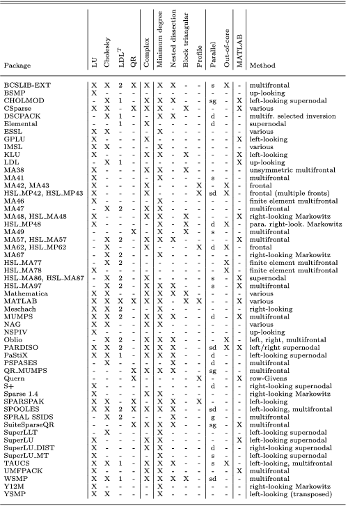
Package authors, references, and availability.
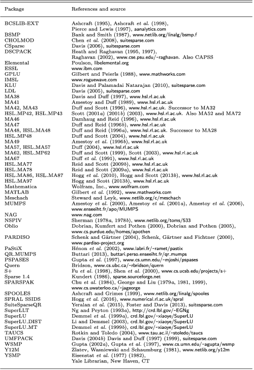
Dongarra maintains an up-to-date list of freely available software at the Netlib website,Footnote 3 including a section on sparse direct solvers. Li’s (Reference Li2013) report focuses solely on sparse direct solvers and is also frequently updated.
Prior software surveys include those of Duff (Reference Duff1984b, Reference Duff and Cowell1984e) and Section 8.6 of Davis (Reference Davis2006). Performance comparisons appear in many articles, but they are the sole focus of several studies, including Duff (Reference Duff, Duff and Stewart1979), Gould and Scott (Reference Gould and Scott2004), and Gould, Scott and Hu (Reference Gould, Scott and Hu2007). Software engineering issues in the design of sparse direct solvers, including object-oriented techniques, have been studied by Ashcraft and Grimes (Reference Ashcraft and Grimes1999), Dobrian, Kumfert and Pothen (Reference Dobrian, Kumfert, Pothen, Bruaset, Langtangen and Quak2000), Scott and Hu (Reference Scott and Hu2007), Sala, Stanley and Heroux (Reference Sala, Stanley and Heroux2008), and Davis (Reference Davis2013).
Acknowledgements
We would like to thank Iain Duff for his comments on a draft of this paper. Portions of this work were supported by the National Science Foundation, Texas A&M University, and Sandia, a multiprogram laboratory operated by Sandia Corporation, a Lockheed Martin Company, for the US Department of Energy under contract DE-AC04-94-AL85000. We would like to thank SIAM for their permission to use material for this paper from Davis’s book, Direct Methods for Sparse Linear Systems, SIAM (2006).