Mechanisms of dynamic wetting failure in the presence of soluble surfactants

Chen-Yu Liu; Marcio S. Carvalho; Satish Kumar

doi:10.1017/jfm.2017.394

Mechanisms of dynamic wetting failure in the presence of soluble surfactants

Published online by Cambridge University Press: 21 July 2017

and

Chen-Yu Liu: Affiliation:
Department of Chemical Engineering and Materials Science, University of Minnesota, Minneapolis, MN 55455, USA
Marcio S. Carvalho*: Affiliation:
Department of Mechanical Engineering, Pontificia Universidade Católica do Rio de Janeiro, Rio de Janeiro, RJ 22451-041, Brazil
Satish Kumar*: Affiliation:
Department of Chemical Engineering and Materials Science, University of Minnesota, Minneapolis, MN 55455, USA
*: †Email addresses for correspondence: kumar030@umn.edu, msc@puc-rio.br
†Email addresses for correspondence: kumar030@umn.edu, msc@puc-rio.br

Article contents

Abstract
Introduction
Hydrodynamic model
Parametric study
Experimental study
Comparison of $Ca^{crit}$ from experiments and model predictions
Conclusions
References

Rights & Permissions

Abstract

A hydrodynamic model and flow visualization experiments are used to understand the mechanisms through which soluble surfactants can influence the onset of dynamic wetting failure. In the model, a Newtonian liquid displaces air in a rectangular channel in the absence of inertia. A Navier-slip boundary condition and constant contact angle are used to describe the dynamic contact line, and surfactants are allowed to adsorb to the interface and moving channel wall (substrate). The Galerkin finite element method is used to calculate steady states and identify the critical capillary number $Ca^{crit}$ at which wetting failure occurs. It is found that surfactant solubility weakens the influence of Marangoni stresses, which tend to promote the onset of wetting failure. Adsorption of surfactants to the substrate can delay the onset of wetting failure due to the emergence of Marangoni stresses that thicken the air film near the dynamic contact line. The experiments indicate that $Ca^{crit}$ increases with surfactant concentration. For the more viscous solutions used, this behaviour can largely be explained by accounting for changes to the mean surface tension and static contact angle produced by surfactants. For the lowest-viscosity solution used, comparison between the model predictions and experimental observations suggests that other surfactant-induced phenomena such as Marangoni stresses may play a more important role.

JFM classification

Materials Processing Flows: Coating Interfacial Flows (free surface): Contact lines Interfacial Flows (free surface): Interfacial Flows (free surface)

Information

Type: Papers
Information: Journal of Fluid Mechanics , Volume 825 , 25 August 2017, pp. 677 - 703
DOI: https://doi.org/10.1017/jfm.2017.394 [Opens in a new window]
Copyright: © 2017 Cambridge University Press

1 Introduction

1.1 Motivation

Dynamic wetting is the displacement of an ambient fluid by a liquid on a solid surface. In coating processes, steady dynamic wetting is a prerequisite for uniform deposition of a liquid layer on a moving substrate (Weinstein & Ruschak Reference Weinstein and Ruschak2004). When the displacement process occurs at a critical substrate speed $U^{crit}$ , the liquid fails to uniformly wet the substrate, resulting in unsteady flow and entrainment of the displaced phase between the liquid and the substrate. If air is the displaced phase, dynamic wetting failure leads to air entrainment: air bubbles are pinched off from a sawtooth-shaped dynamic contact line (DCL) (Burley & Kennedy Reference Burley and Kennedy1976; Benkreira & Khan Reference Benkreira and Khan2008; Vandre, Carvalho & Kumar Reference Vandre, Carvalho and Kumar2014).

Although wetting failure has attracted much attention due to its industrial importance (Miyamoto & Katagiri Reference Miyamoto, Katagiri, Kistler and Schweizer1997; Cohu & Benkreira Reference Cohu and Benkreira1998; Benkreira & Ikin Reference Benkreira and Ikin2010; Vandre, Carvalho & Kumar Reference Vandre, Carvalho and Kumar2012, Reference Vandre, Carvalho and Kumar2013; Sprittles Reference Sprittles2015), relatively little is known about the influence of surfactants on this wetting transition. In addition to being of fundamental interest, this issue is of practical importance since surfactants are used in coating processes to lower surface tension and enhance substrate wettability (Blake Reference Blake1998; Matar & Craster Reference Matar and Craster2009). If the distribution of surfactants along the fluid interface is non-uniform, surface-tension gradients (known as Marangoni stresses) arise and pull fluid from regions of low to high surface tension. Furthermore, the surfactants may be soluble in the bulk liquid, leading to surfactant exchange between the bulk and the fluid interface and substrate.

The objective of the present paper is to investigate the influence of surfactant solubility on dynamic wetting failure using a hydrodynamic model and complementary experiments. As will be discussed below, prior experimental work has reported that surfactants influence the onset of wetting failure, i.e. the critical substrate speed $U^{crit}$ (Deryagin & Levi Reference Deryagin and Levi1964; Burley & Kennedy Reference Burley and Kennedy1976; Gutoff & Kendrick Reference Gutoff and Kendrick1982; Marston et al. Reference Marston, Hawkins, Decent and Simmons2009), but the underlying mechanisms have not been clearly resolved.

1.2 Summary of related prior work

Burley & Kennedy (Reference Burley and Kennedy1976) conducted plunge-coating experiments, where a substrate is pulled through a liquid pool, and reported critical substrate speeds $U^{crit}$ for air entrainment. They found that the addition of surfactant (Teepol detergent) to a glycerol–water mixture lowers the critical substrate speed $U^{crit}$ by 17.5 % but increases the critical capillary number $Ca^{crit}$ by 4 %. The critical capillary number provides a measure of viscous forces relative to surface-tension forces at the onset of wetting failure, and has the definition $Ca^{crit}=\unicode[STIX]{x1D707}U^{crit}/\unicode[STIX]{x1D70E}$ , where $\unicode[STIX]{x1D707}$ is the liquid viscosity and $\unicode[STIX]{x1D70E}$ is the surface tension.

Prior modelling work suggests that $U^{crit}$ and $Ca^{crit}$ can be influenced by surfactants in the following three ways (Liu et al. Reference Liu, Vandre, Carvalho and Kumar2016b ). First, if the surfactants only reduce the equilibrium surface tension, then by dimensional analysis $U^{crit}$ decreases but $Ca^{crit}$ does not change. Second, if the surfactants decrease the static contact angle, both $U^{crit}$ and $Ca^{crit}$ would increase due to an increase in substrate wettability (assuming all other physical properties fixed). Third, if the surfactants produce Marangoni stresses, both $U^{crit}$ and $Ca^{crit}$ would decrease due to the thinning of the air film near the DCL (Liu et al. Reference Liu, Vandre, Carvalho and Kumar2016b ). Note that, in general, all of these phenomena may occur simultaneously.

Although a reduction in equilibrium surface tension ( ${\sim}$ 21.3 %) is observed in the experiments of Burley & Kennedy (Reference Burley and Kennedy1976), the influence of the latter two phenomena on the experimental value of $U^{crit}$ is unclear, since Burley & Kennedy did not report the change in the static contact angle produced by the addition of surfactants. This motivates us to conduct an experimental study in which this change is measured.

In our prior work (Liu et al. Reference Liu, Vandre, Carvalho and Kumar2016b ), we developed a hydrodynamic model to study the influence of Marangoni stresses produced by insoluble surfactants in a parallel-plate geometry where the top boundary is immobile and the bottom substrate moves horizontally at a speed $U$ . Steady interface shapes were tracked as a function of substrate speed, and a critical substrate speed $U^{crit}$ was identified beyond which no two-dimensional (2D) steady-state solutions could be found. This critical substrate speed corresponds to a critical capillary number $Ca^{crit}$ .

The critical capillary number $Ca^{crit}$ arises because capillary-stress gradients due to interface curvature near the DCL are no longer strong enough to provide the pressure gradients needed to pump the receding fluid (air) away from the DCL. The model shows that Marangoni stresses (directed away from the DCL) promote the onset of wetting failure by thinning the air film between the fluid interface and the substrate (Liu et al. Reference Liu, Vandre, Carvalho and Kumar2016b ). The thinner air film leads to larger pressure gradients in the air phase, making it more difficult for pressure gradients due to capillarity to remove the air from the DCL.

The model predictions were then used to interpret the experimental observations of Burley & Kennedy (Reference Burley and Kennedy1976). Since they did not report values of the static contact angles, these quantities had to be estimated. Although both the model and experiments show that surfactants decrease $U^{crit}$ , the model underpredicts the value of $U^{crit}$ by 50 %, suggesting that Marangoni stresses in the system are overestimated. The difference in the value of $U^{crit}$ may result from the assumption of insoluble surfactants in the model, whereas Teepol detergent contains soluble surfactants. In addition, the uncertainty in the experimental values of the static contact angle (as noted above) may also contribute to the difference in the value of $U^{crit}$ . These factors prevent us from drawing more definitive conclusions about the important physical processes at play in the experiments of Burley & Kennedy (Reference Burley and Kennedy1976).

Since surfactant solubility can weaken Marangoni stresses through exchange between the fluid interface and the bulk, one would expect that the predicted $U^{crit}$ from a model accounting for surfactant solubility will be increased and therefore closer to the experimental value. Thus, our prior work provides a strong motivation to develop a model accounting for surfactant solubility and to conduct complementary experiments in which both $U^{crit}$ and the static contact angle are measured.

In addition to transport between the fluid interface and the bulk, surfactants can adsorb to the solid substrate, as illustrated in prior experimental studies on dynamic wetting (Frank & Garoff Reference Frank and Garoff1995; Schunk & Scriven Reference Schunk, Scriven, Kistler and Schweizer1997; Kumar, Maldarelli & Couzis Reference Kumar, Maldarelli and Couzis2006; Bera & Duits Reference Bera, Duits, Cohen Stuart, van den Ende and Mugele2016). The adsorption can occur as surfactants along the interface get carried to the DCL, and it can also occur as surfactants in the bulk liquid get transported to the substrate. Adsorption can influence the surfactant concentration distribution, and thus the surface tension along the fluid interface. To advance fundamental understanding of how this phenomenon influences dynamic wetting failure, it would be useful to incorporate substrate adsorption of surfactants (through the DCL and from the bulk liquid) into our model.

1.3 Overview of present paper

Building on our prior work on insoluble surfactants (Liu et al. Reference Liu, Vandre, Carvalho and Kumar2016b ), we develop a hydrodynamic model accounting for surfactant solubility and substrate adsorption in a parallel-plate geometry. An experimental study including plunge-coating experiments and characterization of liquid properties is conducted. Comparison of the model predictions and experimental observations provides insight into the physical mechanisms through which surfactants influence the onset of dynamic wetting failure. We note that the parallel-plate geometry was used to study dynamic wetting failure in the absence of surfactants, and the predictions of $Ca^{crit}$ show good agreement with experimental observations for a feasible slip-length value (Vandre et al. Reference Vandre, Carvalho and Kumar2012, Reference Vandre, Carvalho and Kumar2013, Reference Vandre, Carvalho and Kumar2014).

The mathematical formulation and solution method for the hydrodynamic model are described in § 2. In § 3, we discuss the influence of surfactant solubility and substrate adsorption on $Ca^{crit}$ . The experimental study is presented in § 4. Comparisons of $Ca^{crit}$ from experiments and the hydrodynamic model are made in § 5. Conclusions are provided in § 6.

2 Hydrodynamic model

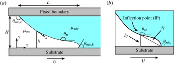
The model problem we consider is illustrated in figure 1(a). A receding fluid is displaced by an advancing liquid within a gap $H$ , where the top boundary is held fixed while the bottom boundary moves horizontally at a speed $U$ . Viscosity is denoted by $\unicode[STIX]{x1D707}$ , with subscripts being used to distinguish between properties of the advancing and receding fluids (i.e. $\unicode[STIX]{x1D707}_{adv}$ and $\unicode[STIX]{x1D707}_{rec}$ ). Symbols $x$ and $y$ represent the Cartesian coordinates, and $s$ is the arclength along the fluid interface (located at $y=h$ ) starting from the static (top) contact line. The horizontal length of the interface is denoted by $L$ .

A schematic displaying the microscopic contact angle $\unicode[STIX]{x1D703}_{mic}$ and the macroscopic contact angle $\unicode[STIX]{x1D703}_{M}$ is shown in figure 1(b). The microscopic angle ( $\unicode[STIX]{x1D703}_{mic}$ ) is formed between the fluid interface and the substrate and serves as a boundary condition in our model. In contrast, the macroscopic angle ( $\unicode[STIX]{x1D703}_{M}$ ) is measured at some distance away from the contact line due to the bending of the interface by viscous forces. In this work, the maximum angle along the fluid interface is designated as $\unicode[STIX]{x1D703}_{M}$ and corresponds to the inflection point (IP) of the fluid interface, whose height and radial distance from the DCL are denoted by $h_{f}$ and $r_{f}$ , respectively. Since the fluid interface contacts both horizontal boundaries, $\unicode[STIX]{x1D703}_{mic,T}$ and $\unicode[STIX]{x1D703}_{mic,B}$ in figure 1(a) represent the microscopic contact angles at the top and bottom boundaries, respectively.

Figure 1.

(a) Schematic of problem geometry. (b) Enlargement of contact-line region. The inflection point (IP) corresponds to the maximum interface angle ( $\unicode[STIX]{x1D703}_{M}$ ), and its height and radial distance are denoted by $h_{f}$ and $r_{f}$ , respectively.

2.1 Hydrodynamics

The following steady Stokes equations describe the velocity $\boldsymbol{v}$ and pressure $p$ in the advancing phase:

(2.1a,b )

$$\begin{eqnarray}\displaystyle \unicode[STIX]{x1D735}\boldsymbol{\cdot }\boldsymbol{v}=0,\quad \unicode[STIX]{x1D735}p=\unicode[STIX]{x1D6FB}^{2}\boldsymbol{v}. & & \displaystyle\end{eqnarray}$$

The characteristic scales $H$ , $U$ and $\unicode[STIX]{x1D707}_{adv}U/H$ are used to non-dimensionalize the lengths, velocities and stresses, respectively.

Since the air phase is long and slender near the onset of wetting failure, lubrication theory can be applied to this phase to greatly reduce computational costs. The resulting one-dimensional (1D) description of the air flow is given by the following equations (Vandre Reference Vandre2013; Liu et al. Reference Liu, Vandre, Carvalho and Kumar2016b ):

(2.2)

$$\begin{eqnarray}\displaystyle & \displaystyle Ah+\frac{1}{2}Bh^{2}+\frac{1}{6}\frac{\text{d}p}{\text{d}s}h^{3}=0, & \displaystyle\end{eqnarray}$$

(2.3)

$$\begin{eqnarray}\displaystyle & \displaystyle \left.\frac{\unicode[STIX]{x2202}u}{\unicode[STIX]{x2202}y}\right|_{s}=B+\frac{\text{d}p}{\text{d}s}h\quad \text{where }A=\frac{\unicode[STIX]{x1D712}h+\unicode[STIX]{x1D712}\unicode[STIX]{x1D706}u_{s}-\displaystyle \frac{1}{2}\frac{\text{d}p}{\text{d}s}h^{2}\unicode[STIX]{x1D706}}{\unicode[STIX]{x1D706}+h},~B=\frac{-\unicode[STIX]{x1D712}+A}{\unicode[STIX]{x1D706}}. & \displaystyle\end{eqnarray}$$

Here $h$ is the interface height, $p$ is the air pressure, $(\unicode[STIX]{x2202}u/\unicode[STIX]{x2202}y)|_{s}$ is the velocity gradient evaluated at the interface, $u$ is the horizontal velocity component, and $u_{\text{s}}$ represents $u$ evaluated at the fluid interface. The symbol $\unicode[STIX]{x1D706}=l_{slip}/H$ is a dimensionless slip length, with $l_{slip}$ being the dimensional slip length, and $\unicode[STIX]{x1D712}=\unicode[STIX]{x1D707}_{rec}/\unicode[STIX]{x1D707}_{adv}$ is the viscosity ratio.

In (2.2) and (2.3), the pressure gradients ( $\text{d}p/\text{d}s$ ) use the quasi-parallel approximation ( $\text{d}x\approx \text{d}s$ ), where $s$ represents the arclength coordinate along the interface (Jacqmin Reference Jacqmin2004; Sbragaglia, Sugiyama & Biferale Reference Sbragaglia, Sugiyama and Biferale2008). We note that this hybrid approach of a 1D description of the receding air and a 2D description of the advancing liquid has been used in our previous work (Vandre Reference Vandre2013; Liu et al. Reference Liu, Vandre, Carvalho and Kumar2016a ,Reference Liu, Vandre, Carvalho and Kumar b ). The predictions of the onset of wetting failure from this hybrid approach are in excellent agreement with those obtained from a model using a 2D description of both the air and liquid flows in the absence of surfactants (Vandre Reference Vandre2013; Liu et al. Reference Liu, Vandre, Carvalho and Kumar2016b ). The reliability of the hybrid approach in the absence of surfactants motivates us to use this approach to study wetting failure in the presence of surfactants.

The following dimensionless boundary conditions are applied along the fluid interface:

(2.4)

$$\begin{eqnarray}\displaystyle & \displaystyle \boldsymbol{t}\boldsymbol{\cdot }\boldsymbol{v}\mid _{adv}=u_{s}, & \displaystyle\end{eqnarray}$$

(2.5)

$$\begin{eqnarray}\displaystyle & \displaystyle \boldsymbol{n}\boldsymbol{\cdot }\boldsymbol{v}=0, & \displaystyle\end{eqnarray}$$

(2.6)

$$\begin{eqnarray}\displaystyle & \displaystyle M\unicode[STIX]{x1D735}_{\boldsymbol{s}}\unicode[STIX]{x1D70E}\boldsymbol{\cdot }\boldsymbol{t}=\boldsymbol{n}\boldsymbol{\cdot }\unicode[STIX]{x1D64F}\boldsymbol{\cdot }\boldsymbol{t}\mid _{adv}-~\boldsymbol{n}\boldsymbol{\cdot }\unicode[STIX]{x1D64F}\boldsymbol{\cdot }\boldsymbol{t}\mid _{rec}, & \displaystyle\end{eqnarray}$$

(2.7)

$$\begin{eqnarray}\displaystyle & \displaystyle \unicode[STIX]{x1D705}(1/Ca+\unicode[STIX]{x1D70E}M)=\boldsymbol{n}\boldsymbol{\cdot }\unicode[STIX]{x1D64F}\boldsymbol{\cdot }\boldsymbol{n}\mid _{adv}-~\boldsymbol{n}\boldsymbol{\cdot }\unicode[STIX]{x1D64F}\boldsymbol{\cdot }\boldsymbol{n}\mid _{rec}. & \displaystyle\end{eqnarray}$$

Equations (2.4) and (2.5) represent the no-slip and no-penetration conditions, and (2.6) and (2.7) correspond to interfacial stress balances in the tangential and normal directions. At the fluid interface, unit normal vector $\boldsymbol{n}$ points towards the air phase and unit tangent vector $\boldsymbol{t}$ is in the same direction as the arclength coordinate $s$ along the interface (figure 1 a).

In (2.6) and (2.7), $\unicode[STIX]{x1D735}_{\boldsymbol{s}}\unicode[STIX]{x1D70E}$ indicates the surface-tension gradient along the interface, $\unicode[STIX]{x1D705}$ corresponds to the interface curvature and $\unicode[STIX]{x1D64F}$ is the Newtonian stress tensor. The parameters $M=(\unicode[STIX]{x1D70E}_{o}-\unicode[STIX]{x1D70E}_{m})/\unicode[STIX]{x1D707}_{adv}U$ and $Ca=\unicode[STIX]{x1D707}_{adv}U/\unicode[STIX]{x1D70E}_{m}$ are the Marangoni and capillary numbers, where $\unicode[STIX]{x1D70E}_{o}$ denotes the surface tension of the solvent (i.e. surfactant-free solution) and $\unicode[STIX]{x1D70E}_{m}$ is the surface tension corresponding to the mean surfactant concentration $\unicode[STIX]{x1D6E4}_{m}$ at the interface. The Marangoni number $M$ gives the relative strength of surface-tension-gradient forces (i.e. Marangoni forces) to viscous forces. When surfactants are absent, $\unicode[STIX]{x1D70E}_{o}=\unicode[STIX]{x1D70E}_{m}$ and the Marangoni stresses are zero. The capillary number $Ca$ provides a measure of the strength of viscous forces relative to surface-tension forces.

A Navier-slip boundary condition is applied along the moving substrate to remove the stress singularity at the DCL (Huh & Scriven Reference Huh and Scriven1971; Dussan Reference Dussan1976; Chan et al. Reference Chan, Srivastava, Marchand, Andreotti, Biferale, Toschi and Snoeijer2013; Sibley, Nold & Kalliadasis Reference Sibley, Nold and Kalliadasis2015; Sprittles Reference Sprittles2017):

(2.8)

$$\begin{eqnarray}\displaystyle \boldsymbol{t}_{\boldsymbol{s}}\boldsymbol{\cdot }(\boldsymbol{v}-\boldsymbol{U})=\unicode[STIX]{x1D706}[\boldsymbol{n}_{s}\boldsymbol{\cdot }\unicode[STIX]{x1D64F}\boldsymbol{\cdot }\boldsymbol{t}_{\boldsymbol{s}}]. & & \displaystyle\end{eqnarray}$$

Here, $\unicode[STIX]{x1D706}$ represents the dimensionless slip length defined earlier and $\boldsymbol{U}$ is the substrate velocity vector. Symbols $\boldsymbol{n}_{\boldsymbol{s}}$ and $\boldsymbol{t}_{\boldsymbol{s}}$ are unit vectors that are normal (pointing towards the fluids) and tangent to the substrate, respectively. This slip boundary condition is able to recover the no-slip condition ( $\boldsymbol{v}\rightarrow \boldsymbol{U}$ ) at distances greater than $l_{slip}$ away from the DCL. For simplicity, we assume that $l_{slip}$ is the same in both the air and liquid phases. The no-slip boundary condition is applied to the top (fixed) boundary and the no-penetration condition is applied to both solid boundaries.

The ends of the fluid interface in the model are set by the microscopic contact angles $\unicode[STIX]{x1D703}_{mic}$ at the static contact line (top) and DCL (bottom) (Blake Reference Blake2006; Snoeijer & Andreotti Reference Snoeijer and Andreotti2013). Although $\unicode[STIX]{x1D703}_{mic}$ may depend on the substrate speed, material properties and flow field (Kistler Reference Kistler and Berg1993; Shikhmurzaev Reference Shikhmurzaev1997; Sui, Ding & Spelt Reference Sui, Ding and Spelt2014; Blake, Fernandez-Toledano & Doyen Reference Blake, Fernandez-Toledano, Doyen and De Coninck2015), here $\unicode[STIX]{x1D703}_{mic}$ is assumed to be constant and the same as the static contact angle $\unicode[STIX]{x1D703}_{s}$ (Lowndes Reference Lowndes1980; Eggers Reference Eggers2005; Vandre et al. Reference Vandre, Carvalho and Kumar2013; Sui et al. Reference Sui, Ding and Spelt2014). This assumption has been used in our prior work on the parallel-plate system in the absence of surfactants (Vandre et al. Reference Vandre, Carvalho and Kumar2013), and the predictions of the onset of wetting failure agree well with experimental observations for a feasible slip-length value.

2.2 Surfactant transport

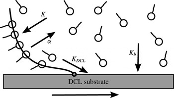
In this work we study the influence of surfactant solubility and substrate adsorption on dynamic wetting failure. As will be discussed below, we use a model involving four parameters that account for adsorption ( $K$ ) and desorption ( $\unicode[STIX]{x1D6FC}$ ) of surfactants between the fluid interface and the bulk, and substrate adsorption through the DCL ( $K_{DCL}$ ) and from the bulk ( $K_{b}$ ). These processes are illustrated in figure 2. More complex models accounting for phenomena such as micelle formation could be developed (e.g. Schunk & Scriven Reference Schunk, Scriven, Kistler and Schweizer1997), but are beyond the scope of the present paper.

Figure 2.

Schematic of surfactant adsorption/desorption near the dynamic contact line (DCL).

In the bulk, surfactant transport is described by a steady convection–diffusion equation,

(2.9)

$$\begin{eqnarray}\displaystyle \boldsymbol{v}\boldsymbol{\cdot }\unicode[STIX]{x1D735}C=\frac{1}{Pe_{b}}\unicode[STIX]{x1D6FB}^{2}C, & & \displaystyle\end{eqnarray}$$

where $C$ represents the dimensionless surfactant concentration in the bulk scaled by a mean bulk concentration $C_{o}$ . The bulk Péclet number $Pe_{b}=UH/D_{b}$ is defined using the bulk diffusion coefficient $D_{b}$ , and shows the strength of surfactant convection relative to diffusion in the bulk.

Since we are interested in the possible influence of substrate adsorption of surfactants on dynamic wetting failure, the no-flux condition for surfactants is applied to the top boundary (figure 1 a). At the right boundary, a fixed dimensionless bulk concentration $C=1$ is applied, acting as a surfactant reservoir. The conditions at the left and bottom boundaries will be discussed below.

A mass flux describes surfactant transport between the bulk and the fluid interface (left boundary of the bulk; figure 1 a). At this location, the flux is given by

(2.10)

$$\begin{eqnarray}\displaystyle -\frac{1}{Pe_{b}}\boldsymbol{n}\boldsymbol{\cdot }\unicode[STIX]{x1D735}C=K(C_{s}-\unicode[STIX]{x1D6E4}), & & \displaystyle\end{eqnarray}$$

where $C_{s}$ is the dimensionless bulk concentration there and $\unicode[STIX]{x1D6E4}$ is the dimensionless surfactant concentration at the interface scaled by the mean surfactant concentration $\unicode[STIX]{x1D6E4}_{m}$ . The solubility number $K=k_{a}\unicode[STIX]{x1D6E4}_{\infty }/U$ shows the ratio of the rates of adsorption (to the fluid interface) and convection, where $k_{a}$ is the adsorption rate constant of surfactants and $\unicode[STIX]{x1D6E4}_{\infty }$ is the concentration at which the interface is saturated (Jensen & Grotberg Reference Jensen and Grotberg1993; Campana & Saita Reference Campana and Saita2006). Following the convention of prior modelling work accounting for surfactant solubility (Jensen & Grotberg Reference Jensen and Grotberg1993; Campana & Saita Reference Campana and Saita2006), the flux is non-dimensionalized by $U\unicode[STIX]{x1D6E4}_{m}/H$ , so the bulk Péclet number $Pe_{b}$ and the solubility number $K$ show up in (2.10). The product of $Pe_{b}$ and $K$ gives the relative strength of adsorption to bulk diffusion. Note that larger $K$ values correspond to less-soluble surfactants (i.e. surfactants tend to adsorb to the fluid interface).

A steady convection–diffusion equation is applied to the fluid interface to describe interfacial surfactant transport:

(2.11)

$$\begin{eqnarray}\displaystyle \unicode[STIX]{x1D735}_{\boldsymbol{s}}\boldsymbol{\cdot }(\boldsymbol{v}_{\boldsymbol{s}}\unicode[STIX]{x1D6E4})=\frac{1}{Pe_{s}}\unicode[STIX]{x1D6FB}_{s}^{2}\unicode[STIX]{x1D6E4}+j_{n},\quad \text{where }j_{n}=\unicode[STIX]{x1D6FC}(C_{s}-\unicode[STIX]{x1D6E4}). & & \displaystyle\end{eqnarray}$$

The symbol $\unicode[STIX]{x1D735}_{\boldsymbol{s}}$ denotes the surface gradient operator, $\boldsymbol{v}_{\boldsymbol{s}}$ is the interface velocity and $j_{n}$ is the flux between the bulk and the interface. The desorption number $\unicode[STIX]{x1D6FC}=k_{d}H/U$ shows the strength of desorption (from the fluid interface) relative to convection, where $k_{d}$ is the desorption rate constant at the fluid interface (Jensen & Grotberg Reference Jensen and Grotberg1993; Campana & Saita Reference Campana and Saita2006). Larger values of $\unicode[STIX]{x1D6FC}$ result in more desorption of surfactants from the fluid interface. The surface Péclet number $Pe_{s}=UH/D_{s}$ is defined using the surface diffusion coefficient $D_{s}$ , and shows the strength of surfactant convection relative to diffusion at the fluid interface. The product of $Pe_{s}$ and $\unicode[STIX]{x1D6FC}$ gives the relative strength of desorption to surface diffusion. Note that the desorption number $\unicode[STIX]{x1D6FC}$ and the solubility number $K$ are related by $\unicode[STIX]{x1D6FC}\unicode[STIX]{x1D6E4}_{m}/HC_{o}=K$ , where the mean bulk concentration $C_{o}$ and the mean interfacial concentration $\unicode[STIX]{x1D6E4}_{m}$ are related by the isotherm $C_{o}=\unicode[STIX]{x1D6E4}_{m}k_{d}/k_{a}\unicode[STIX]{x1D6E4}_{\infty }$ .

As noted in § 1, surfactants can adsorb to the substrate through the DCL or from the bulk liquid. To account for adsorption through the DCL, a mass flux of surfactants at the DCL is used:

(2.12)

$$\begin{eqnarray}\displaystyle -{\displaystyle \frac{1}{Pe_{s}}}\boldsymbol{t}\boldsymbol{\cdot }\unicode[STIX]{x1D735}\unicode[STIX]{x1D6E4}=K_{DCL}\unicode[STIX]{x1D6E4}_{s}, & & \displaystyle\end{eqnarray}$$

where $\unicode[STIX]{x1D6E4}_{s}$ represents the dimensionless surfactant concentration at the DCL and $K_{DCL}=k_{DCL}H/U$ is the DCL adsorption parameter, which shows the relative strength of adsorption (at the DCL) to convection, where $k_{DCL}$ is the adsorption rate constant (Bose Reference Bose and Berg1993; Ramé Reference Ramé2001; Karapetsas, Craster & Matar Reference Karapetsas, Craster and Matar2011). This boundary condition recovers the no-flux condition if $K_{DCL}=0$ , and the product of $Pe_{s}$ and $K_{DCL}$ gives the strength of adsorption (at the DCL) relative to surface diffusion. Note that, since we are interested in the influence of substrate adsorption on wetting failure occurring at the DCL, we assume that surfactants do not deposit onto the top solid boundary. Therefore, the no-flux condition $\boldsymbol{t}\boldsymbol{\cdot }\unicode[STIX]{x1D735}\unicode[STIX]{x1D6E4}=0$ is applied at the top end of the fluid interface.

To describe surfactant adsorption from the bulk to the substrate, a mass flux is applied at the bottom boundary of the bulk (i.e. the interface between the bulk and moving substrate):

(2.13)

$$\begin{eqnarray}\displaystyle -\frac{1}{Pe_{b}}\boldsymbol{n}\boldsymbol{\cdot }\unicode[STIX]{x1D735}C=K_{b}C_{s}. & & \displaystyle\end{eqnarray}$$

Here $C_{s}$ represents the bulk surfactant concentration at the substrate, $\boldsymbol{n}$ is the unit normal vector pointing downwards and $K_{b}=k_{b}H/U$ is the bulk adsorption parameter, which shows the relative strength of adsorption (at the bottom boundary) to convection, where $k_{b}$ is the adsorption rate constant at the substrate (Beacham, Matar & Craster Reference Beacham, Matar and Craster2009; Karapetsas et al. Reference Karapetsas, Craster and Matar2011). If $K_{b}=0$ , there is no adsorption of surfactants on the substrate. The product of $Pe_{b}$ and $K_{b}$ gives the strength of adsorption (at the bottom boundary) relative to bulk diffusion.

The surfactant transport equation (2.11) influences the tangential stress balance (2.6) through an equation of state, a relationship between surface tension and interfacial surfactant concentration. Generally, surface tension depends logarithmically on surfactant concentration (Tricot Reference Tricot, Kistler and Schweizer1997). Here, we assume that the surfactant concentration is dilute enough to apply a linearized equation of state (Ramé Reference Ramé2001; Campana, Di Paolo & Saita Reference Campana, Di Paolo and Saita2004; Campana et al. Reference Campana, Ubal, Giavedoni and Saita2011):

(2.14)

$$\begin{eqnarray}\displaystyle \unicode[STIX]{x1D70E}=1-\unicode[STIX]{x1D6E4}. & & \displaystyle\end{eqnarray}$$

In this equation, surface tension $\unicode[STIX]{x1D70E}$ has been non-dimensionalized using the relation $\unicode[STIX]{x1D70E}^{\prime }=\unicode[STIX]{x1D70E}_{m}+(\unicode[STIX]{x1D70E}_{o}-\unicode[STIX]{x1D70E}_{m})\unicode[STIX]{x1D70E}$ , where $\unicode[STIX]{x1D70E}^{\prime }$ represents the dimensional surface tension (Craster & Matar Reference Craster and Matar2009).

2.3 Solution method

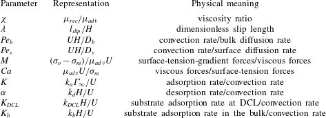
The Galerkin finite element method is used to solve (2.1)–(2.14); for details we refer readers to our previous work (Vandre et al. Reference Vandre, Carvalho and Kumar2012; Liu et al. Reference Liu, Vandre, Carvalho and Kumar2016b ). The key dimensionless model parameters are summarized in table 1. For a given set of parameters, we seek steady-state solutions of the model that include interface shape, surfactant concentration along the interface and in the bulk, pressure in the air phase, and velocity and pressure in the liquid phase. We then track the macroscopic contact angle $\unicode[STIX]{x1D703}_{M}$ (i.e. the maximum contact angle along the interface; figure 1) as a function of the capillary number $Ca$ until a critical capillary number $Ca^{crit}$ is located beyond which we are unable to find a steady-state solution. The value of $Ca^{crit}$ from the solution path is assumed to correspond to the onset of wetting failure.

To isolate the influence of surfactant adsorption/desorption (i.e. $K$ , $\unicode[STIX]{x1D6FC}$ , $K_{DCL}$ and $K_{b}$ ) on wetting failure, we assume neutral and constant microscopic contact angles $\unicode[STIX]{x1D703}_{mic}$ at the top and bottom boundaries of the fluid interface (i.e. $\unicode[STIX]{x1D703}_{mic,T}=\unicode[STIX]{x1D703}_{mic,B}=90^{\circ }$ ) in the parametric study of § 3. In addition, the mean surface tensions $\unicode[STIX]{x1D70E}_{m}$ are kept the same for systems in the absence and presence of surfactants. As a consequence, we can directly compare critical capillary numbers $Ca^{crit}$ for different cases and determine whether a given phenomenon delays or promotes the onset of wetting failure (These assumptions are relaxed in § 4 when we compare model predictions to experimental data.)

We note that, even when $\unicode[STIX]{x1D703}_{mic}=90^{\circ }$ , predictions of $Ca^{crit}$ in the absence of surfactants from the combined approach of a 1D description of the air and a 2D description of the liquid agree well ( ${<}5\,\%$ difference) with those from a model that uses a full 2D description of both the air and liquid phases (Liu et al. Reference Liu, Vandre, Carvalho and Kumar2016b ). This indicates that, even for these large values of $\unicode[STIX]{x1D703}_{mic}$ , a 1D description of the air accurately describes the onset of wetting failure.

Table 1.

Model parameters and corresponding physical meanings.

3 Parametric study

In this section, we perform a parametric study to examine the influence of surfactant solubility and substrate adsorption on dynamic wetting failure. A viscosity ratio of $\unicode[STIX]{x1D712}=5\times 10^{-4}$ is chosen, which corresponds to the case where air is displaced by a liquid having a viscosity of ${\sim}40$ cP. Following our prior work (Liu et al. Reference Liu, Vandre, Carvalho and Kumar2016b ), a dimensionless slip length of $\unicode[STIX]{x1D706}=10^{-4}$ is used. If we take the characteristic length $H$ to be the capillary length $l_{cap}=\sqrt{\unicode[STIX]{x1D70E}_{0}/\unicode[STIX]{x1D70C}g}$ , where $\unicode[STIX]{x1D70C}$ is the liquid density (Vandre et al. Reference Vandre, Carvalho and Kumar2012), then for $l_{cap}\sim 2$ mm this value of $\unicode[STIX]{x1D706}$ corresponds to a dimensional slip length $l_{slip}\sim 0.2~\unicode[STIX]{x03BC}\text{m}$ . Smaller values of $\unicode[STIX]{x1D706}$ would decrease the $Ca^{crit}$ values reported here, but do not affect the qualitative behaviour we observe.

Using a value of $U\sim 0.1~\text{m}~\text{s}^{-1}$ , the value of $H$ noted above and data from prior studies of surfactant adsorption/desorption in aqueous solutions (Chang & Franses Reference Chang and Franses1992, Reference Chang and Franses1995), we find that $Pe_{b}\approx O(10^{5})$ , $Pe_{s}\approx O(10^{4})$ , $M\in [0{-}1]$ , $K\in [10^{-2}{-}10]$ and $\unicode[STIX]{x1D6FC}\in [10{-}10^{5}]$ . To reduce the computational costs associated with resolving high concentration gradients while still remaining in a convection-dominated regime, we use the values of $Pe_{s}=10^{3}$ and $Pe_{b}=10^{4}$ in our calculations. (Reducing these values weakens the influence of Marangoni stresses (see e.g. Liu et al. Reference Liu, Vandre, Carvalho and Kumar2016b ).) We were not able to find values of $K_{DCL}$ and $K_{b}$ in the literature, so we simply vary the values of these parameters to study their qualitative influence on wetting failure.

3.1 Solubility number $K$

Figure 3.

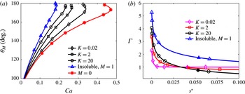
(a) Solution paths for $M=0$ (red asterisks), insoluble surfactants when $M=1$ (blue triangles) and soluble surfactants when $M=1$ with various $K$ values: $K=20$ (black circles), $K=2$ (black squares) and $K=0.02$ (black diamonds). (b) Concentration profiles for insoluble surfactants (blue triangles) and soluble surfactants when $K=20$ (black circles), $K=2$ (red squares) and $K=0.02$ (magenta diamonds). Solid symbols (at $s^{\ast }\approx 0.05$ ) represent the interface IP. Concentration gradients at the IPs are $\text{d}\unicode[STIX]{x1D6E4}/\text{d}s=-12.6$ (insoluble surfactant), $-9.26$ ( $K=20$ ), $-5.30$ ( $K=0$ ) and $-0.08$ ( $K=0.02$ ). Values of other parameters are $\unicode[STIX]{x1D712}=5\times 10^{-4}$ , $\unicode[STIX]{x1D706}=10^{-4}$ , $Pe_{s}=10^{3}$ , $Pe_{b}=10^{4}$ , $\unicode[STIX]{x1D703}_{mic,B}=\unicode[STIX]{x1D703}_{mic,T}=90^{\circ }$ , $\unicode[STIX]{x1D6FC}=350$ and $K_{DCL}=K_{b}=0$ .

The macroscopic contact angle $\unicode[STIX]{x1D703}_{M}$ (figure 1 b) is extracted from the steady interface shape at a given value of the capillary number $Ca$ and is used to construct a steady-state solution path (figure 3 a). By tracking steady-state solutions, we can locate a critical capillary number $Ca^{crit}$ corresponding to a critical substrate speed $U^{crit}$ . Beyond this value of $Ca$ , we are unable to find 2D steady-state solutions, and assume that three-dimensional (3D) and/or transient flows develop. Thus, the value of $Ca^{crit}$ from our calculations is taken to correspond to the onset of wetting failure and can be compared to experimental measurements.

We consider in this section the influence of the solubility number $K$ . For our parametric study, we fix the desorption number $\unicode[STIX]{x1D6FC}$ to a value of 350. We also neglect the influence of substrate adsorption and thus set $K_{DCL}=K_{b}=0$ .

Figure 3(a) shows solution paths for several different cases: $M=0$ , insoluble surfactants when $M=1$ , and soluble surfactants when $M=1$ and several different values of $K$ . The results for insoluble surfactants are obtained using the model developed in our previous work (Liu et al. Reference Liu, Vandre, Carvalho and Kumar2016b ), where an additional mass-conservation constraint is applied along the fluid interface. Figure 3(a) demonstrates that the presence of Marangoni stresses (i.e. the cases where $M=1$ ) decreases $Ca^{crit}$ and thus promotes the onset of wetting failure, which is consistent with the finding in our previous work (Liu et al. Reference Liu, Vandre, Carvalho and Kumar2016b ).

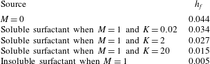
As noted in § 1, Marangoni stresses promote the onset of wetting failure by thinning the air film between the fluid interface and the substrate (Liu et al. Reference Liu, Vandre, Carvalho and Kumar2016b ). This leads to larger air-pressure gradients and makes it more difficult for capillary-stress gradients to pump air away from the DCL. Direct evidence of the thinning of the air film is given in table 2, where the dimensionless film thicknesses $h_{f}$ (figure 1) are shown for the different cases in figure 3(a) when $Ca=0.15$ .

Figure 4.

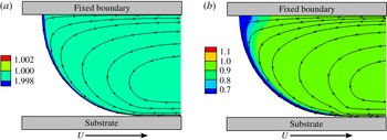
Concentration contours and streamlines for soluble surfactants when (a) $M=1$ , $K=0.02$ and $Ca=0.237$ , and (b) $M=1$ , $K=20$ and $Ca=0.340$ . Note that $Ca=Ca^{crit}$ in both cases. Other parameter values are the same as in figure 3.

Table 2.

Dimensionless film thicknesses $h_{f}$ for the different cases in figure 3(a) when $Ca=0.15$ . Other parameter values are the same as in figure 3(a).

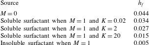
As expected, surfactant solubility decreases Marangoni effects via transport between the fluid interface and the bulk. The $Ca^{crit}$ values for soluble surfactants are larger than the value for insoluble surfactants. In addition, $Ca^{crit}$ decreases as the solubility number $K$ increases, meaning that more adsorption of surfactants to the fluid interface (i.e. less-soluble surfactant) results in stronger Marangoni effects. Fitting the model predictions in figure 3(a) yields a power-law relationship between $Ca^{crit}$ and $K$ , $Ca^{crit}\approx 0.28K^{-0.054}$ . We note that the above results are for $\unicode[STIX]{x1D703}_{mic,B}=90^{\circ }$ . Our prior work on insoluble surfactants shows that changes in $\unicode[STIX]{x1D703}_{mic,B}$ (i.e. substrate wettability) from $45^{\circ }$ to $135^{\circ }$ lead to ${\sim}$ 30 % decrease in $Ca^{crit}$ (Liu et al. Reference Liu, Vandre, Carvalho and Kumar2016b ); we would expect similar behaviour for soluble surfactants.

Figure 3(b) shows the corresponding surfactant concentration profiles along the fluid interface. The concentration is shown as a function of $s^{\ast }$ , the arclength coordinate starting from the DCL. In all cases, the surfactant concentration $\unicode[STIX]{x1D6E4}$ reaches a maximum at $s^{\ast }=0$ , meaning that surfactants accumulate at the DCL. This is because the advancing liquid flow carries surfactants towards the DCL. In the advancing phase, the bottom substrate drags the liquid as it moves to the right. As a consequence, liquid near the fluid interface flows towards the substrate to conserve mass, resulting in a rolling-flow pattern (figure 4) similar to those observed in prior experimental and computational work (Benkreira Reference Benkreira2004; Benkreira & Ikin Reference Benkreira and Ikin2010; Vandre et al. Reference Vandre, Carvalho and Kumar2012; Liu et al. Reference Liu, Vandre, Carvalho and Kumar2016b ). Note that, as the solubility number $K$ decreases, the surfactant concentration at the DCL ( $s^{\ast }=0$ ) also decreases.

The solid symbols in figure 3(b) represent the interface IP. From our previous work on insoluble surfactants (Liu et al. Reference Liu, Vandre, Carvalho and Kumar2016b ), we found that Marangoni stresses directed away from the DCL (i.e. negative concentration gradient at the IP) will promote the onset of wetting failure by thinning the air film between the interface and the substrate. In figure 3(b), the case of insoluble surfactants shows the most negative concentration gradient, meaning that Marangoni effects are the strongest and the $Ca^{crit}$ value is the smallest among all the cases shown. In addition, the absolute value of the concentration gradient decreases as $K$ decreases (see values in figure caption). This is because the adsorption of surfactants from the bulk to the fluid interface becomes weaker as $K$ decreases, resulting in less surfactant accumulation at the DCL.

Figure 4 shows contour plots of the concentration field along with streamlines for soluble surfactants when $K=0.02$ and $K=20$ at $Ca^{crit}$ . Owing to adsorption at the fluid interface, the bulk concentration near the interface is lower than that far away from the interface. In addition, as $K$ increases, adsorption of surfactants becomes stronger, making the low-concentration region larger (figure 4 b).

3.2 Desorption number $\unicode[STIX]{x1D6FC}$

Figure 5.

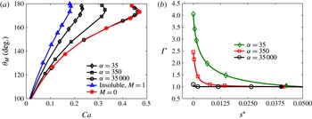
(a) Solution paths for $M=0$ (red asterisks), insoluble surfactants when $M=1$ (blue triangles) and soluble surfactants when $M=1$ with various $\unicode[STIX]{x1D6FC}$ values: $\unicode[STIX]{x1D6FC}=3.5\times 10^{4}$ (black circles), $\unicode[STIX]{x1D6FC}=350$ (black squares) and $\unicode[STIX]{x1D6FC}=35$ (black diamonds). (b) Concentration profiles for soluble surfactants $M=1$ when $\unicode[STIX]{x1D6FC}=35$ (green diamonds), $\unicode[STIX]{x1D6FC}=350$ (red squares) and $\unicode[STIX]{x1D6FC}=3.5\times 10^{4}$ (black circles). Solid symbols (at $s^{\ast }\approx 0.0375$ ) represent the interface IP. Concentration gradients at the IPs are $\text{d}\unicode[STIX]{x1D6E4}/\text{d}s=-7.14$ ( $\unicode[STIX]{x1D6FC}=35$ ), $-0.89$ ( $\unicode[STIX]{x1D6FC}=350$ ) and $-0.0089$ ( $\unicode[STIX]{x1D6FC}=3.5\times 10^{4}$ ). Values of other parameters are $\unicode[STIX]{x1D712}=5\times 10^{-4}$ , $\unicode[STIX]{x1D706}=10^{-4}$ , $Pe_{s}=10^{3}$ , $Pe_{b}=10^{4}$ , $\unicode[STIX]{x1D703}_{mic,B}=\unicode[STIX]{x1D703}_{mic,T}=90^{\circ }$ , $K=0.2$ and $K_{DCL}=K_{b}=0$ .

In figure 5(a), we show solution paths for $M=0$ , insoluble surfactants when $M=1$ , and soluble surfactants when $M=1$ and different values of $\unicode[STIX]{x1D6FC}$ . Here, we fix the value of the solubility number $K$ to a value of 0.2, and again neglect substrate adsorption ( $K_{DCL}=K_{b}=0$ ). As can be seen, $Ca^{crit}$ increases as the desorption number $\unicode[STIX]{x1D6FC}$ increases, meaning that more desorption of surfactants leads to weaker Marangoni effects. In particular, when $\unicode[STIX]{x1D6FC}=3.5\times 10^{4}$ , the solution path as well as the $Ca^{crit}$ value approach those for $M=0$ , indicating that Marangoni stresses are negligible. Fitting the model predictions in figure 5(a) yields a power-law relationship between $Ca^{crit}$ and $\unicode[STIX]{x1D6FC}$ , $Ca^{crit}\approx 0.18\unicode[STIX]{x1D6FC}^{0.091}$ .

Figure 5(b) shows the corresponding concentration profiles along the fluid interface for soluble surfactants. The surfactant concentration is largest near the DCL, and its magnitude decreases as $\unicode[STIX]{x1D6FC}$ increases (i.e. as desorption increases and Marangoni stresses become weaker). In addition, the concentration gradient at the IP decreases as $\unicode[STIX]{x1D6FC}$ increases. For $\unicode[STIX]{x1D6FC}=3.5\times 10^{4}$ , the concentration profile is nearly uniform, consistent with the observation above that the solution path for this case is similar to that for $M=0$ . The contour plots for different values of $\unicode[STIX]{x1D6FC}$ are similar to those for different values of $K$ (figure 4), so are not shown.

3.3 DCL adsorption parameter $K_{DCL}$

Figure 6.

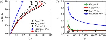
(a) Solution paths for $M=0$ (red asterisks), insoluble surfactants when $M=1$ (blue triangles) and soluble surfactants when $M=1$ with various $K_{DCL}$ values: $K_{DCL}=0$ (black diamonds), $K_{DCL}=0.3$ (black squares) and $K_{DCL}=1.2$ (black circles). (b) Concentration profiles for insoluble surfactants (blue triangles) and soluble surfactants when $K_{DCL}=0$ (green diamonds), $K_{DCL}=0.3$ (red squares) and $K_{DCL}=1.2$ (black circles). Solid symbols (at $s^{\ast }\approx 0.0375$ ) represent the interface IP. Concentration gradients at the IPs are $\text{d}\unicode[STIX]{x1D6E4}/\text{d}s=-12.6$ (insoluble surfactant), $-0.89$ ( $K_{DCL}=0$ ), $-0.28$ ( $K_{DCL}=0.3$ ) and $0.16$ ( $K_{DCL}=1.2$ ). Values of other parameters are $\unicode[STIX]{x1D712}=5\times 10^{-4}$ , $\unicode[STIX]{x1D706}=10^{-4}$ , $Pe_{s}=10^{3}$ , $Pe_{b}=10^{4}$ , $\unicode[STIX]{x1D703}_{mic,B}=90^{\circ }$ , $K=0.2$ , $\unicode[STIX]{x1D6FC}=350$ and $K_{b}=0$ .

We now turn to the effects of surfactant adsorption to the substrate, first considering the case of adsorption through the DCL while neglecting adsorption from the bulk ( $K_{b}=0$ ). Figure 6(a) shows solution paths for several different cases: $M=0$ , insoluble surfactants when $M=1$ , and soluble surfactants when $M=1$ and several different values of $K_{DCL}$ . Clearly, $Ca^{crit}$ increases as $K_{DCL}$ increases, suggesting that adsorption of surfactants through the DCL has a significant effect on Marangoni stresses. Surprisingly, when $K_{DCL}=1.2$ the $Ca^{crit}$ value becomes larger than that for $M=0$ , meaning that the onset of wetting failure is delayed. Fitting the model predictions in figure 6(a) yields a power-law relationship between $Ca^{crit}$ and $K_{DCL}$ , $Ca^{crit}\approx 0.50K_{DCL}^{0.17}$ .

Figure 6(b) shows the corresponding concentration profiles along the fluid interface. Similar to figure 3(b), the case of insoluble surfactants shows the most negative concentration gradient at the IP, whereas the absolute values of the concentration gradients are greatly reduced in the case of soluble surfactants (see values in figure caption). In addition, as $K_{DCL}$ increases, more surfactant transfers from the fluid interface to the substrate through the DCL ( $s^{\ast }=0$ ), decreasing the surfactant concentration at the DCL. Notably, if $K_{DCL}$ is large enough (e.g. $K_{DCL}=1.2$ ), the concentration gradient $\text{d}\unicode[STIX]{x1D6E4}/\text{d}s$ at the IP even changes its sign from negative to positive. For these large values of $K_{DCL}$ , the substrate serves as a surfactant ‘sink’ and prevents accumulation of surfactant there. As a consequence, the direction of the concentration gradient and Marangoni stresses at the DCL reverses.

Our previous work (Liu et al. Reference Liu, Vandre, Carvalho and Kumar2016b ) showed that Marangoni stresses directed away from the DCL (i.e. negative concentration gradient at the IP) promote the onset of wetting failure by thinning the air film. The reversal of the direction of Marangoni stresses suggests that the air film is thickened, resulting in a delay in the onset of wetting failure. From our results, we found that at the same $Ca$ value (e.g. $Ca=0.47$ ) the characteristic air film thickness ( $h_{f}$ in figure 1 b) for $K_{DCL}=1.2$ ( $h_{f}=0.0086$ ) is larger than that for $M=0$ ( $h_{f}=0.0067$ ), corroborating the argument that thickening of the air film (by Marangoni stresses directed towards the DCL) delays the onset of wetting failure.

Since $K_{DCL}$ changes the surfactant concentration primarily near the DCL, it has a negligible effect on the concentration distribution in the bulk. Thus, contour plots for different values of $K_{DCL}$ are not shown.

3.4 Bulk adsorption parameter $K_{b}$

Figure 7.

(a) Solution paths for $M=0$ (red asterisks), insoluble surfactants when $M=1$ (blue triangles) and soluble surfactants when $M=1$ with various $K_{b}$ values: $K_{b}=0$ (black diamonds), $K_{b}=0.05$ (black squares) and $K_{b}=0.1$ (black circles). (b) Concentration profiles for insoluble (blue triangles) and soluble surfactants when $K_{b}=0$ (green diamonds), $K_{b}=0.05$ (red squares) and $K_{b}=0.1$ (black circles). Solid symbols (at $s^{\ast }\approx 0.0375$ ) represent the interface IP. Concentration gradients at the IPs are $\text{d}\unicode[STIX]{x1D6E4}/\text{d}s=-0.57$ ( $K_{b}=0$ ), $2.11$ ( $K_{b}=0.05$ ) and $2.80$ ( $K_{b}=0.1$ ). Values of other parameters are $\unicode[STIX]{x1D712}=5\times 10^{-4}$ , $\unicode[STIX]{x1D706}=10^{-4}$ , $Pe_{s}=10^{3}$ , $Pe_{b}=10^{4}$ , $\unicode[STIX]{x1D703}_{mic,B}=90^{\circ }$ , $K=0.2$ , $\unicode[STIX]{x1D6FC}=550$ and $K_{DCL}=0$ .

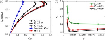
We now consider surfactant adsorption from the bulk to the substrate while neglecting adsorption through the DCL ( $K_{DCL}=0$ ). In figure 7(a), we show solution paths for $M=0$ , insoluble surfactants when $M=1$ , and soluble surfactants when $M=1$ and several different values of $K_{b}$ . As can be seen, $Ca^{crit}$ increases as $K_{b}$ increases, implying that surfactant adsorption from the bulk can strongly influence Marangoni stresses. Notably, the value of $Ca^{crit}$ for soluble surfactants with $K_{b}=0.1$ is larger than that for $M=0$ , suggesting that adsorption of surfactants from the bulk can delay the onset of wetting failure. Fitting the model predictions in figure 7(a) yields a power-law relationship between $Ca^{crit}$ and $K_{b}$ , $Ca^{crit}\approx 0.63K_{b}^{0.10}$ .

Figure 7(b) shows the corresponding concentration profiles along the fluid interface. Interestingly, when $K_{b}\neq 0$ , a local minimum in the concentration profiles appears, suggesting that Marangoni stresses change direction along the fluid interface (i.e. from directed away to directed towards the DCL as $s^{\ast }$ increases). Because surfactants carried by the flow in the advancing phase cannot be transported through the DCL ( $s^{\ast }=0$ ) since $K_{DCL}=0$ , they accumulate there, leading to the largest concentration values at $s^{\ast }=0$ . These values decrease as $K_{b}$ increases.

Adsorption to the substrate acts as a surfactant sink and decreases the bulk concentration near the substrate. As a result, surfactants on the fluid interface near the bottom substrate desorb to equilibrate with the surfactant concentration in the bulk, resulting in a local minimum in the interfacial concentration profile. The minimum becomes more pronounced as $K_{b}$ (adsorption to the substrate) increases. Note that in § 3.3 no concentration minimum is created by substrate adsorption through the DCL, so the Marangoni stresses do not change sign.

To understand how the concentration minimum influences $Ca^{crit}$ , it is instructive to compare the concentration gradient values ( $\text{d}\unicode[STIX]{x1D6E4}/\text{d}s$ ) at the IP: $-0.57$ ( $K_{b}=0$ ), $2.11$ ( $K_{b}=0.05$ ) and $2.80$ ( $K_{b}=0.1$ ). When $K_{b}=0$ , the Marangoni stresses point away from the DCL (due to the negative value of $\text{d}\unicode[STIX]{x1D6E4}/\text{d}s$ ), indicating that Marangoni stresses promote the onset of wetting failure.

When $\text{d}\unicode[STIX]{x1D6E4}/\text{d}s$ is positive, one might expect that Marangoni stresses will delay the onset of wetting failure (i.e. lead to a larger value of $Ca^{crit}$ compared to $M=0$ ). However, when $K_{b}=0.05$ , $Ca^{crit}$ is still smaller than that for $M=0$ . This is because the negative concentration gradients near the DCL (i.e. Marangoni stresses pointing away from the DCL) compete with the positive ones near the IP (i.e. Marangoni stresses pointing towards the DCL). In this case ( $K_{b}=0.05$ ), the negative concentration gradients near the DCL dominate and lead to a decrease in $Ca^{crit}$ (compared to $M=0$ ). As the value of $K_{b}$ further increases, the concentration gradients near the IP become more positive. When $K_{b}=0.1$ , the positive concentration gradients near the IP dominate. As a result, the onset of wetting failure is delayed and $Ca^{crit}$ becomes larger than that for $M=0$ .

The competition between the Marangoni stresses is reflected in the behaviour of the characteristic air film thickness ( $h_{f}$ in figure 1 b). Recall that, as the air film is thinned, the onset of wetting failure is promoted since capillary-stress gradients become less effective at removing air from the DCL (Liu et al. Reference Liu, Vandre, Carvalho and Kumar2016b ). When $Ca=0.46$ , the air film for soluble surfactants with $K_{b}=0.1$ ( $h_{f}=0.0072$ ) is thicker than that for $M=0$ ( $h_{f}=0.0070$ ) and $K_{b}=0.05$ ( $h_{f}=0.0066$ ), suggesting that $Ca^{crit}$ for $K_{b}=0.1$ has the largest value among these three cases, consistent with figure 7(a). For $K_{b}=0.05$ , the film thickness is thinner than that for $M=0$ , meaning that $Ca^{crit}$ will be smaller than that for $M=0$ , again consistent with figure 7(a).

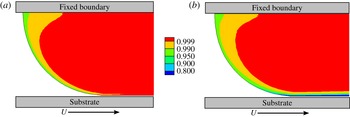
Figure 8 shows contour plots of the concentration field for soluble surfactants when $K_{b}=0$ and $K_{b}=0.1$ at $Ca^{crit}$ . Similar to figure 4, the bulk concentration near the interface is lower than that far away from the interface. However, when surfactants in the bulk adsorb to the substrate, a region of low concentration appears near the substrate (figure 8 b).

4 Experimental study

To complement our model predictions, we have also conducted an experimental study. Below we describe the experimental apparatus and liquid characterization. A comparison between the experimental data and model predictions is performed in § 5.

4.1 Experimental apparatus

Figure 8.

Concentration contours for soluble surfactants when (a) $M=1$ , $K_{b}=0$ and $Ca=0.35$ , and (b) $M=1$ , $K_{b}=0.1$ and $Ca=0.50$ . Note that $Ca=Ca^{crit}$ in both cases. Other parameter values are the same as in figure 7.

Figure 9.

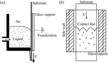
(a) Schematic of experimental apparatus, which is similar to the design used in Vandre et al. (Reference Vandre, Carvalho and Kumar2014). (b) Front view of apparatus. Contact-line behaviour is visualized through a glass support plate located to the right of the substrate in panel (a).

A schematic of our experimental apparatus is shown in figure 9(a) (Vandre et al. Reference Vandre, Carvalho and Kumar2014). A transparent polyethylene terephthalate (PET) tape moves through a vessel, with one side of the tape in contact with liquid and the other in contact with a glass support. A $125~\unicode[STIX]{x03BC}\text{m}$ thick and 2 inch wide tape is used for all of the experiments reported in this paper. Before an experiment (i.e. tape is immobile), ${\sim}$ 250 ml of liquid is fed through an inlet located at the back of the vessel. Once the vessel is filled with the desired amount of liquid, the inlet is shut off to avoid creating flows in the vessel during an experiment. A high-speed camera is used to visualize contact-line behaviour through the glass support as the tape speed increases (figure 9 b). A plate can be inserted into the tank to confine the meniscus (Vandre et al. Reference Vandre, Carvalho and Kumar2014), but since we wish to focus on the influence of surfactants in the absence of meniscus confinement, the plate is not used here.

The vessel acts like a plunge-coating tank, similar to the apparatus used by Burley & Kennedy (Reference Burley and Kennedy1976). However, the advantage of our design is that one can directly visualize DCL behaviour. In this work, wetting failure is signalled by the appearance of triangular air films at the DCL as the tape speed increases. The corresponding tape speed is designated as the critical substrate speed $U^{crit}$ . 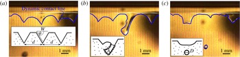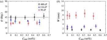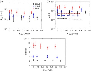For each liquid, three experiments are carried out to assess the reproducibility of the critical speed. The triangular films are sensitive to disturbances and can quickly rupture, leaving behind air bubbles that are entrained in the bulk liquid. More details about the shape and thickness of these films in the absence of surfactants can be found in Vandre et al. (Reference Vandre, Carvalho and Kumar2014). The key features of the air films (e.g. width, thickness and spacing) are largely insensitive to the presence of surfactants (see appendix A).

4.2 Liquid characterization

Figure 10.

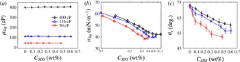
Characterization of solutions with various sodium dodecyl sulfate (SDS) concentrations: (a) viscosity, (b) surface tension and (c) static contact angle on PET substrates for $\unicode[STIX]{x1D707}_{liq}=400$ cP (black diamonds), $\unicode[STIX]{x1D707}_{liq}=116$ cP (blue triangles) and $\unicode[STIX]{x1D707}_{liq}=50$ cP (red squares).

The liquids used in this study are glycerol–water solutions. The surfactant used is sodium dodecyl sulfate (SDS) (Sigma-Aldrich ReagentPlus^®). During solution preparation, we found that the solubility of SDS in glycerol–water mixtures is low, especially for highly viscous solutions. Small SDS clumps remain in the mixture even after stirring and waiting overnight. As a result, SDS is dissolved in deionized water first, and pure glycerol is added afterwards. The resulting glycerol–water–SDS mixture is stirred and left to rest overnight to dissipate large air bubbles and equilibrate with the laboratory temperature.

Three liquid viscosities, $\unicode[STIX]{x1D707}_{liq}=400$ cP, 116 cP and 50 cP, are used in this study. The viscosities are obtained from an AR-G2 rheometer (TA Instruments), which shows that the viscosity is independent of shear rate in the range between $1~\text{s}^{-1}$ and $900~\text{s}^{-1}$ . The mean liquid viscosities are plotted as a function of surfactant concentration $C_{SDS}$ in figure 10(a), and do not change with the addition of surfactants throughout the range of $C_{SDS}$ investigated. Note that, in the plunge-coating experiments, the shear rate (based on the web speed and capillary length) is between $10~\text{s}^{-1}$ and $100~\text{s}^{-1}$ . The value of $U^{crit}$ increases as $\unicode[STIX]{x1D707}_{liq}$ decreases, meaning that more tape needs to be used in a given experiment. Because of the limited supply of tape, we do not use liquids with a viscosity below 50 cP.

The surface tensions of the solutions are obtained from a Krüss K10ST digital tensiometer (figure 10 b). As expected, the surface tension decreases as the surfactant concentration increases. We can determine the critical micelle concentration (CMC) from the point where the slope of the surface-tension curve changes as $C_{SDS}$ increases. The CMC for each liquid viscosity is $C_{SDS}\approx 0.94$ wt% ( $\unicode[STIX]{x1D707}_{liq}=400$ cP), $C_{SDS}\approx 0.77$ wt% ( $\unicode[STIX]{x1D707}_{liq}=116$ cP) and $C_{SDS}\approx 0.47$ wt% ( $\unicode[STIX]{x1D707}_{liq}=50$ cP). This increase in CMC with glycerol content (i.e. liquid viscosity) is consistent with prior experimental observations for SDS and other ionic/non-ionic surfactants (Cantu et al. Reference Cantu, Corti, Degiorgio, Hoffmann and Ulbricht1987; Takisawa et al. Reference Takisawa, Thomason, Bloor and Wyn-Jones1993; Ruiz, Diaz-Lopez & Aguiar Reference Ruiz, Diaz-Lopez and Aguiar2008). Note that solutions with $C_{SDS}<\text{CMC}$ are used in the plunge-coating experiments to be more consistent the dilute-surfactant assumption of the model.

Figure 10(b) also shows that the surface tension depends on the liquid viscosity. At a fixed surfactant concentration, a lower liquid viscosity corresponds to a smaller value of surface tension. This is because there is more aqueous surfactant solution in the less-viscous liquids. This finding is similar to what was observed for SDS and sodium tetradecyl sulfate (STS) in prior experiments (Fainerman, Makievski & Miller Reference Fainerman, Makievski and Miller1993; Staggemeier et al. Reference Staggemeier, Collier, Prazen and Synovec2005).

Static contact angles on the PET tape are measured by the sessile drop method using a Krüss DSA goniometer. The influence of surfactants on the contact angles is shown in figure 10(c). Owing to the reduction in surface tension, the contact angle decreases as $C_{SDS}$ increases, consistent with Young’s equation (Tricot Reference Tricot, Kistler and Schweizer1997). Similarly, since a less-viscous liquid corresponds to a smaller value of surface tension, the contact-angle values decrease as the liquid viscosity decreases. Note that the static contact angles reported here will be used as the boundary condition at the DCL in our model ( $\unicode[STIX]{x1D703}_{mic,B}$ in figure 1 a).

5 Comparison of $Ca^{crit}$ from experiments and model predictions

Figure 11.

(a) Critical speed $U^{crit}$ and (b) critical capillary number $Ca^{crit}$ for $\unicode[STIX]{x1D707}_{liq}=400$ cP (black diamonds), $\unicode[STIX]{x1D707}_{liq}=116$ cP (blue triangles) and $\unicode[STIX]{x1D707}_{liq}=50$ cP (red squares). The solid lines in panel (a) are drawn to aid visualization. The dashed lines in panel (b) correspond to power-law fits of $Ca^{crit}$ for three liquids: $Ca^{crit}\sim C_{SDS}^{0.055}$ (black, $\unicode[STIX]{x1D707}_{liq}=400$ cP), $Ca^{crit}\sim C_{SDS}^{0.051}$ (blue, $\unicode[STIX]{x1D707}_{liq}=116$ cP) and $Ca^{crit}\sim C_{SDS}^{0.076}$ (red, $\unicode[STIX]{x1D707}_{liq}=50$ cP). For reference, the values of $Ca^{crit}$ when $C_{SDS}=0$ are 0.545 ( $\unicode[STIX]{x1D707}_{liq}=400$ cP), 0.379 ( $\unicode[STIX]{x1D707}_{liq}=116$ cP) and 0.336 ( $\unicode[STIX]{x1D707}_{liq}=50$ cP).

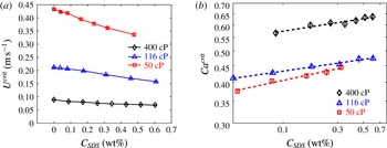
Air entrainment occurs above a critical substrate speed $U^{crit}$ , at which the contact line forms triangular air films. Air bubbles are generated when the films rupture. The speed $U^{crit}$ from our experiments (§ 4) is plotted as a function of SDS concentration $C_{SDS}$ for the three liquid viscosities (figure 11 a). As can be seen, the critical speed decreases as the surfactant concentration increases at a given liquid viscosity. In addition, surfactants have a larger effect on $U^{crit}$ at lower liquid viscosities.

We also note that lower critical speeds occur at higher liquid viscosities, consistent with prior experiments (Vandre et al. Reference Vandre, Carvalho and Kumar2014). This can be understood by considering the case where surfactants are absent. At fixed interfacial tension and microscopic contact angle, higher liquid viscosities promote greater interface bending, leading to larger capillary-stress gradients and air-pressure gradients (due to a thinner air film). However, the air-pressure gradients increase more rapidly than the capillary-stress gradients as the liquid viscosity increases, so wetting failure occurs at a lower critical speed (Liu Reference Liu2017).

Figure 11(b) shows the corresponding values of the critical capillary number $Ca^{crit}$ . As can be seen, $Ca^{crit}$ increases with the liquid viscosity, consistent with prior experimental observations (Burley & Kennedy Reference Burley and Kennedy1976; Burley & Jolly Reference Burley and Jolly1984; Kistler Reference Kistler and Berg1993; Benkreira Reference Benkreira2004; Vandre et al. Reference Vandre, Carvalho and Kumar2014). In addition, at a fixed liquid viscosity $Ca^{crit}$ increases with $C_{SDS}$ , showing the same trend as that reported by Burley & Kennedy (Reference Burley and Kennedy1976).

To generate predictions of $Ca^{crit}$ from the model, the viscosity ratio $\unicode[STIX]{x1D712}=\unicode[STIX]{x1D707}_{air}/\unicode[STIX]{x1D707}_{liq}$ is calculated based on the air and liquid viscosities. The Marangoni number $M=(\unicode[STIX]{x1D70E}_{o}-\unicode[STIX]{x1D70E}_{m})/\unicode[STIX]{x1D707}_{liq}U^{crit}$ is obtained using the surface tension $\unicode[STIX]{x1D70E}_{m}$ and the surface tension $\unicode[STIX]{x1D70E}_{o}$ of the corresponding glycerol–water mixture when $C_{SDS}=0$ . Note that the value of $M$ increases (from ${\sim}$ 0.1 to 1) as $C_{SDS}$ increases due to the changes in $\unicode[STIX]{x1D70E}_{m}$ and $U^{crit}$ . The microscopic contact angles $\unicode[STIX]{x1D703}_{mic,B}$ at the DCL are set equal to the corresponding static contact angles (§ 4.2) at each value of $C_{SDS}$ .

The capillary length $l_{cap}=\sqrt{\unicode[STIX]{x1D70E}_{m}/\unicode[STIX]{x1D70C}g}$ is used as the characteristic length scale $H$ when calculating various parameters (table 1), where $\unicode[STIX]{x1D70C}$ and $g$ are the liquid density and the gravitational acceleration, respectively. For the liquids used here, $l_{cap}\sim 2{-}2.3~\text{mm}$ . Since $l_{cap}$ is much less than the tank width ( ${\sim}$ 10 cm), the effects of meniscus confinement are negligible and it is appropriate to take $l_{cap}$ as the characteristic length scale (Vandre et al. Reference Vandre, Carvalho and Kumar2012, Reference Vandre, Carvalho and Kumar2014). The Reynolds numbers in the advancing and receding phases (based on the substrate velocity and capillary length) in the experiments are at most ${\sim}$ 20 and ${\sim}$ 65, respectively, which are much below the values where inertia significantly affects the value of $Ca^{crit}$ (Vandre et al. Reference Vandre, Carvalho and Kumar2013).

Since exact experimental values of the diffusion coefficients $D_{b}$ and $D_{s}$ and the rate constants for adsorption $k_{a}$ and desorption $k_{d}$ are difficult to measure, we estimate these values from prior experimental studies of aqueous solutions (Chang & Franses Reference Chang and Franses1992, Reference Chang and Franses1995). These values are used to calculate the Péclet numbers $Pe_{b}$ and $Pe_{s}$ , the solubility number $K$ and the desorption number $\unicode[STIX]{x1D6FC}$ in our experiments. Inevitably, this creates a high level of uncertainty, since our liquids are more viscous than those used in prior studies. Note that, although we use the same dimensional values of $k_{a}$ and $k_{d}$ for all calculations, $K$ and $\unicode[STIX]{x1D6FC}$ change as $C_{SDS}$ does due to the changes in $U^{crit}$ and $l_{cap}$ . The values of $Pe_{b}$ and $Pe_{s}$ also change as $C_{SDS}$ does, but, because these are always very large, for simplicity we set $Pe_{b}=10^{5}$ and $Pe_{s}=10^{4}$ . This corresponds to a convection-dominated limit where the results are insensitive to further increases in the Péclet numbers (Liu et al. Reference Liu, Vandre, Carvalho and Kumar2016b ). Since we do not have any experimental data for the parameters controlling surfactant adsorption to the substrate, $K_{DCL}$ and $K_{b}$ , we set these parameters to zero.

Figure 12.

Comparison of model predictions with experimental data for (a) $\unicode[STIX]{x1D707}_{liq}=400$ cP, (b) $\unicode[STIX]{x1D707}_{liq}=116$ cP and (c) $\unicode[STIX]{x1D707}_{liq}=50$ cP. In each panel, symbols correspond to $Ca^{crit}$ from our experiments (black diamonds), our model when $M=0$ (red circles) and our model when $M\neq 0$ (blue squares). Dashed lines correspond to power-law fits of each data set. See appendix B for model parameters for each data point.

The dimensionless slip length $\unicode[STIX]{x1D706}$ ( $\unicode[STIX]{x1D706}\leqslant 10^{-5}$ ) is treated as an adjustable parameter. For a given liquid, its value is varied until the prediction for $Ca^{crit}$ at $C_{SDS}=0$ agrees with the experimental value. This value of $\unicode[STIX]{x1D706}$ is then used for all calculations at non-zero $C_{SDS}$ . In this work, $\unicode[STIX]{x1D706}\sim 10^{-6}{-}10^{-5}$ , which corresponds to dimensional slip lengths ${\sim}2{-}20~\text{nm}$ , values comparable to those used in our prior work on wetting failure in the absence of surfactants (Vandre et al. Reference Vandre, Carvalho and Kumar2012, Reference Vandre, Carvalho and Kumar2013, Reference Vandre, Carvalho and Kumar2014).

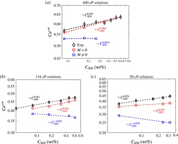
In figure 12, we plot the experimental values of $Ca^{crit}$ for each liquid as a function of $C_{SDS}$ , along with the corresponding model predictions. In addition to the predictions for $M\neq 0$ , we also show predictions from calculations where we set $M=0$ . The $M=0$ predictions allow us to assess how well the experimental behaviour can be described by simply accounting for changes to the mean surface tension and static contact angle. To facilitate comparison between the experimental values and model predictions, we also fit power-law relationships to the data in the plots. These are shown with dashed lines and the power-law exponents are given in the plots.

For the 400 cP case, figure 12(a) shows that the predictions when $M=0$ agree much better with the experimental data compared to the predictions when $M\neq 0$ . The predictions for $M\neq 0$ indicate that $Ca^{crit}$ is nearly independent of $C_{SDS}$ , whereas the predictions for $M=0$ show that $Ca^{crit}$ increases as $C_{SDS}$ does, consistent with the experimental data.

We have also performed calculations (not shown for brevity) where we have varied the parameters controlling surfactant adsorption to the fluid interface, $K$ and $\unicode[STIX]{x1D6FC}$ , over a physically reasonable range of values. However, we are unable to match the experimental values of $Ca^{crit}$ . Similarly, reducing the value of $\unicode[STIX]{x1D703}_{mic,B}$ to account for the possibility that the local surfactant concentration at the DCL may be higher than the given value of $C_{SDS}$ also does not lead to agreement with the experimental data. This suggests that, for the 400 cP solutions, the simplest explanation consistent with the experimental data is that the increase in $Ca^{crit}$ with $C_{SDS}$ can largely be understood just by accounting for changes to the mean surface tension and static contact angle when surfactants are present.

For the $116~\text{cP}$ case, figure 12(b) shows that the predictions for $M=0$ are again in much better agreement with the experimental data than those for $M\neq 0$ . Indeed, in this case, the $M\neq 0$ calculations predict that $Ca^{crit}$ decreases as $C_{SDS}$ increases, which is opposite to what is observed experimentally. The predictions for $M=0$ are slightly below the experimental data, but can be brought into better agreement if a lower value of $\unicode[STIX]{x1D703}_{mic,B}$ is used (to account for a higher local surfactant concentration at the DCL, as noted above). Varying the values of $K$ , $\unicode[STIX]{x1D6FC}$ and $\unicode[STIX]{x1D703}_{mic,B}$ over physically reasonable ranges does not lead to a match between the $M\neq 0$ predictions and the experimental data. As with the 400 cP solutions, this suggests that the experimental data can largely be explained just by accounting for changes to the mean surface tension and static contact angle when surfactants are present.

For the 50 cP solutions, figure 12(c) shows that the $M=0$ predictions are once more in better agreement with the experimental data, and that the $M\neq 0$ calculations again predict that $Ca^{crit}$ decreases as $C_{SDS}$ increases. However, the discrepancy between the $M=0$ calculations and the experimental data is larger compared to the other two liquid viscosities. Using a lower values of $\unicode[STIX]{x1D703}_{mic,B}$ in the $M=0$ calculations raises the $Ca^{crit}$ values, but does not bring them into agreement with the experimental data. Thus, for these solutions, surfactant-related phenomena (e.g. substrate adsorption) other than changes to the mean surface tension and static contact angle may be playing a more important role. Indeed, as the solutions become less viscous, Marangoni stresses would be expected to become more influential (e.g. the values of $M$ are generally larger for the 50 cP solutions compared to the 400 cP solutions (appendix B)). However, as noted in § 4.2, experimental limitations have prevented us from studying solutions with viscosities lower than 50 cP.

For all of the cases shown in figure 12, the model predictions for $M\neq 0$ are lower than the experimental values. Since Marangoni stresses tend to lower the value of $Ca^{crit}$ (§ 3), this suggests that the model may overestimate the importance of Marangoni stresses, possibly due to the use of a linear equation of state and linear rate laws for surfactant adsorption (Chang & Franses Reference Chang and Franses1995; Schunk & Scriven Reference Schunk, Scriven, Kistler and Schweizer1997; Alvarez et al. Reference Alvarez, Vogus, Walker and Anna2012). It is also possible that the slip length may vary with surfactant concentration, or the assumption of a Navier-slip law with constant microscopic contact angle may break down in the presence of surfactants (Zhu & Granick Reference Zhu and Granick2002; Cheikh & Koper Reference Cheikh and Koper2003; Henry et al. Reference Henry, Neto, Evans, Biggs and Craig2004; Kunert & Harting Reference Kunert and Harting2008; Sochi Reference Sochi2011). Finally, we note that, if the parameters controlling surfactant adsorption to the substrate, $K_{DCL}$ and $K_{b}$ , are made non-zero ( $K_{DCL}\approx O(1)$ , $K_{b}\approx O(0.1)$ ), it is possible to obtain agreement between the model predictions and experimental data. However, experimental values of these parameters are unknown, preventing us from drawing definitive conclusions about the role of surfactant adsorption. Resolution of these issues will require methods of imaging surfactant concentration distributions along the fluid interface and substrate and in the bulk, and improved characterization of surfactant adsorption kinetics (Fallest et al. Reference Fallest, Lichtenberger, Fox and Daniels2010; Swanson et al. Reference Swanson, Strickland, Shearer and Daniels2015).

Overall, the results from this section indicate that, for the more viscous solutions, the increase in $Ca^{crit}$ with surfactant concentration can largely be explained by accounting for changes to the mean surface tension and static contact angle (This is also consistent with our observation in appendix A that the air-film characteristics are not significantly affected by surfactant concentration.) For the solution with the lowest viscosity, other surfactant-induced phenomena (as described above) may become important, but more comprehensive experiments are needed to elucidate the underlying physical mechanisms.

6 Conclusions

In this work we have used a hydrodynamic model and complementary experiments to gain insight into the physical mechanisms through which surfactants influence the onset of dynamic wetting failure. Our parametric study in § 3 demonstrates how surfactant solubility weakens the influence of Marangoni stresses, and elucidates the influence of various parameters controlling surfactant adsorption to the fluid interface and substrate. Comparison of the model predictions to our experimental observations (§ 5) reveals that, for the more viscous solutions we used, changes to the mean surface tension and static contact angle appear to be largely responsible for the increase in $Ca^{crit}$ with surfactant concentration. For the solution with the lowest viscosity, other surfactant-induced phenomena may become important, but more comprehensive experiments are needed to definitively establish this.

Our results point to the need for imaging of surfactant concentration distributions and better characterization of surfactant adsorption kinetics. There is especially a need for measuring adsorption to substrates, since our results in § 3 raise the possibility that substrate adsorption could be used to delay the onset of wetting failure. Such studies are not only of fundamental interest, but also important for understanding the influence of surfactants in industrially important flows such as curtain coating (Marston et al. Reference Marston, Hawkins, Decent and Simmons2009; Liu et al. Reference Liu, Vandre, Carvalho and Kumar2016a ).

Acknowledgements

This material is based upon work supported by the National Science Foundation under grant no. CBET-1434016. We thank E. Vandre for numerous helpful discussions, 3M™ for the kind donation of PET tapes, and W. J. Suszynski for assistance with the experiments. We are grateful to the Minnesota Supercomputing Institute (MSI) at the University of Minnesota for providing computational resources.

Appendix A. Air-film characteristics

In this work, the critical speed $U^{crit}$ corresponding to dynamic wetting failure is determined by gradually increasing the tape speed until triangular air films form at the dynamic contact line (DCL). The films are sensitive to disturbances and can quickly rupture, leaving behind air bubbles that are entrained in the bulk liquid. In this section, we characterize the films in the presence of surfactants.

Figure 13.

Evolution of the air film at the onset of air entrainment: (a) triangular air films with width $W$ , angle $\unicode[STIX]{x1D713}$ and spacing $d$ ; (b) local rupture of air film with area $A$ ; and (c) formation of a spherical air bubble with diameter $D$ . The schematic in each panel represents an idealization of each state. The blue solid line denotes the dynamic contact line. The liquid viscosity $\unicode[STIX]{x1D707}_{liq}=400~\text{cP}$ and the critical speed $U^{crit}=0.082~\text{m}~\text{s}^{-1}$ . The time lapse between panels is ${\approx}$ 30 ms.

Figure 13 shows three characteristic stages near the DCL at the onset of air entrainment. First, sawtooth-shaped triangular air films appear at the DCL. Each air ‘vee’ can be represented by an isosceles triangle of angle $\unicode[STIX]{x1D713}$ with a width $W$ . The distance between the apexes of adjacent triangles is denoted by $d$ . Second, disturbances cause the elongated air film to locally re-wet the substrate. The re-wetted region grows, resulting in an irregular film of area $A$ connecting with the meniscus (figure 13 b). Finally, a portion of the air film breaks off and forms a spherical bubble with diameter $D$ due to surface-tension forces (figure 13 c). The following sections discuss the influence of surfactants on the shape (§ A.1), thickness and spacing (§ A.2) of the air film.

A.1 Shape

Figure 14.

The effect of SDS concentration $C_{SDS}$ on the triangular air film formed at $Ca^{crit}$ as characterized by (a) angle $\unicode[STIX]{x1D713}$ and (b) width $W$ (refer to figure 13 for the definition of $\unicode[STIX]{x1D713}$ and $W$ ). In each panel, symbols correspond to solutions with different viscosities: $\unicode[STIX]{x1D707}_{liq}=400~\text{cP}$ (black diamonds), $\unicode[STIX]{x1D707}_{liq}=116~\text{cP}$ (blue triangles) and $\unicode[STIX]{x1D707}_{liq}=50~\text{cP}$ (red squares). The dashed line in panel (a) represents $45^{\circ }$ .

Figure 14 demonstrates the influence of surfactants on the characteristic angle $\unicode[STIX]{x1D713}$ and width $W$ of the triangular air films. Interestingly, the addition of surfactants does not significantly change the values of $\unicode[STIX]{x1D713}$ and $W$ . However, $\unicode[STIX]{x1D713}$ and $W$ depend on the liquid viscosity. The angle $\unicode[STIX]{x1D713}$ has a larger value at a higher liquid viscosity, whereas the width $W$ has a larger value at a lower liquid viscosity. These findings are consistent with prior work in the absence of surfactants (Vandre et al. Reference Vandre, Carvalho and Kumar2014). At lower viscosity, the decrease in the angle $\unicode[STIX]{x1D713}$ can be attributed to an edge effect caused by the tape since the air film is wider.

A.2 Thickness and spacing

Figure 15.

(a) Estimated air-film thickness $h_{exp}$ , (b) comparison of the dimensionless film thickness from the experiments $h$ and the height of the inflection point $h_{f}$ from our model, and (c) spacing $d$ of triangular air films at different liquid viscosities: $\unicode[STIX]{x1D707}_{liq}=400~\text{cP}$ (black diamonds), $\unicode[STIX]{x1D707}_{liq}=116~\text{cP}$ (blue triangles) and $\unicode[STIX]{x1D707}_{liq}=50~\text{cP}$ (red squares). In panel (b), the dotted line (50 cP), dashed line (116 cP) and dashed-dotted line (400 cP) represent model predictions of $h_{f}$ when $M=0$ . Note that the $y$ axis in panel (b) is dimensionless.

Air-film thickness can be estimated from visualizations of the evolution of the air films, as illustrated in figure 13. At the early stage of the rupture process (figure 13 b), the meniscus is connected with an irregular air film with volume $A\times h_{exp}$ , where $h_{exp}$ represents the height of the air film defined by area $A$ . Since the diameter $D$ of a spherical air bubble can be easily measured (figure 13 c), the film thickness $h_{exp}$ can be approximated as $h_{exp}=\unicode[STIX]{x03C0}D^{3}/6A$ .

Figure 15(a) shows the estimated film thickness $h_{exp}$ at different surfactant concentrations. We found that the variation of $h_{exp}$ values is small through the range of $C_{SDS}$ investigated. However, the liquid viscosity has a larger effect on $h_{exp}$ values with a higher viscosity corresponding to a smaller $h_{exp}$ value, consistent with the experimental observations in prior work (Vandre et al. Reference Vandre, Carvalho and Kumar2014). The change in the $h_{exp}$ values is a consequence of the interaction between capillary and viscous stresses. As the liquid viscosity increases, the interface can bend more near the DCL, generating larger capillary-stress gradients that lead to a thinner air film (Vandre et al. Reference Vandre, Carvalho and Kumar2014).

Figure 15(b) shows the comparison between the dimensionless film thickness $h=h_{exp}/l_{cap}$ from the experiments and the height of the inflection point $h_{f}$ from our model when $M=0$ . Note that $h_{exp}$ is non-dimensionalized by the capillary length $l_{cap}$ . As can be seen, the variation of $h_{f}$ values is small through the range of $C_{SDS}$ , showing a similar trend to that of the dimensionless film thickness $h$ . We note that, since $h_{f}$ does not necessarily equal the value of $h$ estimated from the experiments, the values of $h_{f}$ may be different from those of $h$ .

As expected, the addition of surfactants does not significantly change the values of the spacing $d$ (figure 15 c). The value of $d$ is mainly influenced by the liquid viscosity, consistent with prior work in the absence of surfactants (Vandre et al. Reference Vandre, Carvalho and Kumar2014).

Appendix B. Model parameters in figure 12

Model parameters in each panel:

(a) $\unicode[STIX]{x1D712}=4.48\times 10^{-5}$ , $\unicode[STIX]{x1D706}=9.07\times 10^{-6}$ , $Pe_{s}=10^{4}$ , $Pe_{b}=10^{5}$ , $K_{DCL}=K_{b}=0$ for each model result. For $M=0$ (red circles), concentration $=[0.086,0.173,0.345,0.517]$ wt%, $\unicode[STIX]{x1D6FC}=[7.64,7.83,8.58,8.95]\times 10^{4}$ , $K=[3.65,3.74,4.10,4.28]\times 10^{1}$ and $\unicode[STIX]{x1D703}_{mic,B}=[71^{\circ },68^{\circ },64^{\circ },61^{\circ }]$ . For $M=[0.22,0.35,0.47]$ (blue squares), concentration $=[0.086,0.173,0.259]$ wt%, $\unicode[STIX]{x1D6FC}=[7.64,7.83,8.24]\times 10^{4}$ , $K=[3.65,3.74,3.94]\times 10^{1}$ and $\unicode[STIX]{x1D703}_{mic,B}=[71^{\circ },68^{\circ },66^{\circ }]$ .

(b) $\unicode[STIX]{x1D712}=1.55\times 10^{-4}$ , $\unicode[STIX]{x1D706}=3.25\times 10^{-6}$ , $Pe_{s}=10^{4}$ , $Pe_{b}=10^{5}$ , $K_{DCL}=K_{b}=0$ for each model result. For $M=0$ (red circles), concentration $=[0.081,0.176,0.310,0.458,0.607]$ wt%, $\unicode[STIX]{x1D6FC}=[3.05,3.16,3.41,3.69,3.97]\times 10^{4}$ , $K=[1.46,1.51,1.63,1.76,1.90]\times 10^{1}$ and $\unicode[STIX]{x1D703}_{mic,B}=[68^{\circ },66^{\circ },63^{\circ },59^{\circ },56^{\circ }]$ . For $M=[0.36,0.51,1,1.3]$ (blue squares), concentration $=[0.081,0.176,0.458,0.607]$ wt%, $\unicode[STIX]{x1D6FC}=[3.05,3.16,3.69,3.97]\times 10^{4}$ , $K=[1.46,1.51,1.76,1.90]\times 10^{1}$ and $\unicode[STIX]{x1D703}_{mic,B}=[68^{\circ },66^{\circ },59^{\circ },56^{\circ }]$ .

(c) $\unicode[STIX]{x1D712}=3.58\times 10^{-4}$ , $\unicode[STIX]{x1D706}=2\times 10^{-6}$ , $Pe_{s}=10^{4}$ , $Pe_{b}=10^{5}$ , $K_{DCL}=K_{b}=0$ for each model result. For $M=0$ (red circles), concentration $=[0.040,0.080,0.239,0.319]$ wt%, $\unicode[STIX]{x1D6FC}=[1.48,1.50,1.66,1.73]\times 10^{4}$ , $K=[7.09,7.18,7.94,8.29]$ and $\unicode[STIX]{x1D703}_{mic,B}=[67^{\circ },62^{\circ },58^{\circ },54^{\circ }]$ . For $M=[0.38,1,1.2]$ (blue squares), concentration $=$ [0.040, 0.239, 0.319] wt%, $\unicode[STIX]{x1D6FC}=[1.48,1.66,1.73]\times 10^{4}$ , $K=[7.09,7.94,8.29]$ and $\unicode[STIX]{x1D703}_{mic,B}=[67^{\circ },58^{\circ },54^{\circ }]$ .

For all of the model predictions, $k_{a}=3\times 10^{4}~\text{m}^{3}~\text{mol}^{-1}~\text{s}$ , $k_{d}=2.73\times 10^{6}~\text{s}^{-1}$ , $D_{b}=10^{-9}~\text{m}^{2}~\text{s}^{-1}$ and $D_{s}=10^{-8}~\text{m}^{2}~\text{s}^{-1}$ (Chang & Franses Reference Chang and Franses1992, Reference Chang and Franses1995).

References

Alvarez, N. J., Vogus, D. R., Walker, L. M. & Anna, S. L. 2012 Using bulk convection in a microtensiometer to approach kinetic-limited surfactant dynamics at fluid–fluid interfaces. J. Colloid Interface Sci. 372 (1), 183–191.Google Scholar

Beacham, D. R., Matar, O. K. & Craster, R. V. 2009 Surfactant-enhanced rapid spreading of drops on solid surfaces. Langmuir 25 (24), 14174–14181.Google Scholar

Benkreira, H. 2004 The effect of substrate roughness on air entrainment in dip coating. Chem. Engng Sci. 59 (13), 2745–2751.Google Scholar

Benkreira, H. & Ikin, J. B. 2010 Dynamic wetting and gas viscosity effects. Chem. Engng Sci. 65 (5), 1790–1796.Google Scholar

Benkreira, H. & Khan, M. I. 2008 Air entrainment in dip coating under reduced air pressures. Chem. Engng Sci. 63 (2), 448–459.Google Scholar

Bera, B., Duits, M. H. G., Cohen Stuart, M. A., van den Ende, D. & Mugele, F. 2016 Surfactant induced autophobing. Soft Matt. 12, 4562–4571.Google Scholar

Blake, T. D.1998 Coating processes. US patent 5792515.Google Scholar

Blake, T. D. 2006 The physics of moving wetting lines. J. Colloid Interface Sci. 299 (1), 1–13.Google Scholar

Blake, T. D., Fernandez-Toledano, J.-C., Doyen, G. & De Coninck, J. 2015 Forced wetting and hydrodynamic assist. Phys. Fluids 27 (11), 112101.Google Scholar

Bose, A. 1993 Wetting by solutions. In Wettability (ed. Berg, J. C.), pp. 149–181. Marcel Dekker.Google Scholar

Burley, R. & Jolly, R. P. S. 1984 Entrainment of air into liquids by a high speed continuous solid surface. Chem. Engng Sci. 39 (9), 1357–1372.Google Scholar

Burley, R. & Kennedy, B. S. 1976 An experimental study of air entrainment at a solid/liquid/gas interface. Chem. Engng Sci. 31, 901–911.Google Scholar

Campana, D. M., Di Paolo, J. & Saita, F. A. 2004 A 2-D model of Rayleigh instability in capillary tubes – surfactant effects. Intl J. Multiphase Flow 30, 431–454.Google Scholar

Campana, D. M. & Saita, F. A. 2006 Numerical analysis of the Rayleigh instability in capillary tubes: the influence of surfactant solubility. Phys. Fluids 18 (2), 022104.Google Scholar

Campana, D. M., Ubal, S., Giavedoni, M. D. & Saita, F. A. 2011 A deeper insight into the dip coating process in the presence of insoluble surfactants: a numerical analysis. Phys. Fluids 23 (5), 052102.CrossRef Google Scholar

Cantu, L., Corti, M., Degiorgio, V., Hoffmann, H. & Ulbricht, W. 1987 Nonionic micelles in mixed water–glycerol solvent. J. Colloid Interface Sci. 116 (2), 384–389.CrossRef Google Scholar

Chan, T. S., Srivastava, S., Marchand, A., Andreotti, B., Biferale, L., Toschi, F. & Snoeijer, J. H. 2013 Hydrodynamics of air entrainment by moving contact lines. Phys. Fluids 25 (7), 074105.Google Scholar

Chang, C.-H. & Franses, E. I. 1992 Modified Langmuir–Hinshelwood kinetics for dynamic adsorption of surfactants at the air/water interface. Colloids Surf. 69, 189–201.Google Scholar

Chang, C.-H. & Franses, E. I. 1995 Adsorption dynamics of surfactants at the air/water interface: a critical review of mathematical models, data, and mechanisms. Colloids Surf., A 100, 1–45.Google Scholar

Cheikh, C. & Koper, G. 2003 Stick–slip transition at the nanometer scale. Phys. Rev. Lett. 91 (15), 156102.Google Scholar

Cohu, O. & Benkreira, H. 1998 Entrainment of air by a solid surface plunging into a non-Newtonian liquid. AIChE J. 44 (11), 2360–2368.Google Scholar

Craster, R. V. & Matar, O. K. 2009 Dynamics and stability of thin liquid films. Rev. Mod. Phys. 81 (3), 1131–1198.Google Scholar

Deryagin, B. M. & Levi, S. M. 1964 Film Coating Theory: Physical Chemistry of Coating. Focal Press.Google Scholar

Dussan, V. E. B. 1976 The moving contact line: the slip boundary condition. J. Fluid Mech. 77 (4), 665–684.CrossRef Google Scholar

Eggers, J. 2005 Existence of receding and advancing contact lines. Phys. Fluids 17 (8), 082106.Google Scholar

Fainerman, V. B., Makievski, A. V. & Miller, R. 1993 The measurement of dynamic surface tensions of highly viscous liquids by the maximum bubble pressure method. Colloids Surf. A 75 (6), 229–235.Google Scholar

Fallest, D. W., Lichtenberger, A. M., Fox, C. J. & Daniels, K. E. 2010 Fluorescent visualization of a spreading surfactant. New J. Phys. 12, 073029.Google Scholar

Frank, B. & Garoff, S. 1995 Origins of the complex motion of advancing surfactant solutions. Langmuir 11 (18), 87–93.Google Scholar

Gutoff, E. B. & Kendrick, C. E. 1982 Dynamic contact angles. AlChE J. 28 (3), 459–466.Google Scholar

Henry, C. L., Neto, C., Evans, D. R., Biggs, S. & Craig, V. S. J. 2004 The effect of surfactant adsorption on liquid boundary slippage. Physica A 339 (1), 60–65.Google Scholar

Huh, C. & Scriven, L. E. 1971 Hydrodynamic model of steady movement of a solid/liquid/fluid contact line. J. Colloid Interface Sci. 35 (1), 85–101.CrossRef Google Scholar

Jacqmin, D. 2004 Onset of wetting failure in liquid–liquid systems. J. Fluid Mech. 517, 209–228.Google Scholar

Jensen, O. E. & Grotberg, J. B. 1993 The spreading of heat or soluble surfactant along a thin liquid film. Phys. Fluids A 5 (1), 58–68.Google Scholar

Karapetsas, G., Craster, R. V. & Matar, O. K. 2011 On surfactant-enhanced spreading and superspreading of liquid drops on solid surfaces. J. Fluid Mech. 670, 5–37.Google Scholar

Kistler, S. F. 1993 Hydrodynamics of wetting. In Wettability (ed. Berg, J. C.), pp. 311–429. Marcel Dekker.Google Scholar

Kumar, N., Maldarelli, C. & Couzis, A. 2006 An infrared spectroscopy study of the hydrogen bonding and water restructuring as a trisiloxane superspreading surfactant adsorbs onto an aqueous-hydrophobic surface. Colloids Surf. A 277, 98–106.Google Scholar

Kunert, C. & Harting, J. 2008 On the effect of surfactant adsorption and viscosity change on apparent slip in hydrophobic microchannels. Prog. Comput. Fluid Dyn. 8 (1–4), 197–205.Google Scholar

Liu, C.-Y.2017 Onset of dynamic wetting failure in the presence of surfactants. PhD thesis, University of Minnesota.Google Scholar

Liu, C.-Y., Vandre, E., Carvalho, M. S. & Kumar, S. 2016a Dynamic wetting failure and hydrodynamic assist in curtain coating. J. Fluid Mech. 808, 290–315.Google Scholar

Liu, C.-Y., Vandre, E., Carvalho, M. S. & Kumar, S. 2016b Dynamic wetting failure in surfactant solutions. J. Fluid Mech. 789, 285–309.Google Scholar

Lowndes, J. 1980 The numerical simulation of the steady movement of a fluid meniscus in a capillary tube. J. Fluid Mech. 101 (3), 631–646.Google Scholar

Marston, J. O., Hawkins, V., Decent, S. P. & Simmons, M. J. H. 2009 Influence of surfactant upon air entrainment hysteresis in curtain coating. Exp. Fluids 46, 549–558.Google Scholar

Matar, O. K. & Craster, R. V. 2009 Dynamics and stability of thin liquid films. Rev. Mod. Phys. 81 (3), 1131–1198.Google Scholar

Miyamoto, K. & Katagiri, Y. 1997 Curtain coating. In Liquid Film Coating (ed. Kistler, S. & Schweizer, P. M.), pp. 463–494. Chapman & Hall.Google Scholar

Ramé, E. 2001 The spreading of surfactant-laden liquids with surfactant transfer through the contact line. J. Fluid Mech. 440, 205–234.Google Scholar

Ruiz, C. C., Diaz-Lopez, L. & Aguiar, J. 2008 Micellization of sodium dodecyl sulfate in glycerol aqueous mixtures. J. Dispersion Sci. Technol. 29 (2), 266–273.Google Scholar

Sbragaglia, M., Sugiyama, K. & Biferale, L. 2008 Wetting failure and contact line dynamics in a Couette flow. J. Fluid Mech. 614, 471–493.Google Scholar

Schunk, P. R. & Scriven, L. E. 1997 Surfactant effects in coating processes. In Liquid Film Coating (ed. Kistler, S. & Schweizer, P. M.), pp. 495–536. Chapman & Hall.Google Scholar

Shikhmurzaev, Y. D. 1997 Moving contact lines in liquid/liquid/solid systems. J. Fluid Mech. 334, 211–249.Google Scholar

Sibley, D. N., Nold, A. & Kalliadasis, S. 2015 The asymptotics of the moving contact line: cracking an old nut. J. Fluid Mech. 764, 445–462.Google Scholar

Snoeijer, J. H. & Andreotti, B. 2013 Moving contact lines: scales, regimes, and dynamical transitions. Annu. Rev. Fluid Mech. 45, 269–292.Google Scholar

Sochi, T. 2011 Slip at fluid–solid interface. Polym. Rev. 51 (4), 309–340.Google Scholar

Sprittles, J. E. 2015 Air entrainment in dynamic wetting: Knudsen effects and the influence of ambient air pressure. J. Fluid Mech. 769, 444–481.Google Scholar

Sprittles, J. E. 2017 Kinetic effects in dynamic wetting. Phys. Rev. Lett. 118 (11), 114502.Google Scholar

Staggemeier, B. A., Collier, T. O., Prazen, B. J. & Synovec, R. E. 2005 Effect of solution viscosity on dynamic surface tension detection. Anal. Chim. Acta 534, 79–87.Google Scholar

Sui, Y., Ding, H. & Spelt, P. D. 2014 Numerical simulations of flows with moving contact lines. Annu. Rev. Fluid Mech. 46, 97–119.Google Scholar

Swanson, E. R., Strickland, S. L., Shearer, M. & Daniels, K. E. 2015 Surfactant spreading on a thin liquid film: reconciling models and experiments. J. Engng Maths 94, 63–79.Google Scholar

Takisawa, N., Thomason, M., Bloor, D. M. & Wyn-Jones, E. 1993 Ultrasonic relaxation and electrochemical studies of the micellization of sodium decyl sulfate and decyltrimethylammonium bromide in glycerol/water mixtures. J. Colloid Interface Sci. 157 (1), 77–81.Google Scholar

Tricot, Y.-M. 1997 Surfactants: static and dynamic surface tension. In Liquid Film Coating (ed. Kistler, S. & Schweizer, P. M.), pp. 99–136. Chapman & Hall.Google Scholar

Vandre, E. A.2013 Onset of dynamic wetting failure: the mechanics of high-speed fluid displacement. PhD thesis, University of Minnesota.Google Scholar

Vandre, E., Carvalho, M. S. & Kumar, S. 2012 Delaying the onset of dynamic wetting failure through meniscus confinement. J. Fluid Mech. 707, 496–520.Google Scholar

Vandre, E., Carvalho, M. S. & Kumar, S. 2013 On the mechanism of wetting failure during fluid displacement along a moving substrate. Phys. Fluids 25 (10), 102103.CrossRef Google Scholar

Vandre, E., Carvalho, M. S. & Kumar, S. 2014 Characteristics of air entrainment during dynamic wetting failure along a planar substrate. J. Fluid Mech. 747, 119–140.Google Scholar

Weinstein, S. J. & Ruschak, K. J. 2004 Coating flows. Annu. Rev. Fluid Mech. 36 (1), 29–53.Google Scholar

Zhu, Y. & Granick, S. 2002 No-slip boundary condition switches to partial slip when fluid contains surfactant. Langmuir 18 (26), 10058–10063.Google Scholar

Figure 1.(a) Schematic of problem geometry. (b) Enlargement of contact-line region. The inflection point (IP) corresponds to the maximum interface angle ($\unicode[STIX]{x1D703}_{M}$), and its height and radial distance are denoted by $h_{f}$ and $r_{f}$, respectively.

Figure 2.Schematic of surfactant adsorption/desorption near the dynamic contact line (DCL).

Table 1.Model parameters and corresponding physical meanings.

Figure 3.(a) Solution paths for $M=0$ (red asterisks), insoluble surfactants when $M=1$ (blue triangles) and soluble surfactants when $M=1$ with various $K$ values: $K=20$ (black circles), $K=2$ (black squares) and $K=0.02$ (black diamonds). (b) Concentration profiles for insoluble surfactants (blue triangles) and soluble surfactants when $K=20$ (black circles), $K=2$ (red squares) and $K=0.02$ (magenta diamonds). Solid symbols (at $s^{\ast }\approx 0.05$) represent the interface IP. Concentration gradients at the IPs are $\text{d}\unicode[STIX]{x1D6E4}/\text{d}s=-12.6$ (insoluble surfactant), $-9.26$ ($K=20$), $-5.30$ ($K=0$) and $-0.08$ ($K=0.02$). Values of other parameters are $\unicode[STIX]{x1D712}=5\times 10^{-4}$, $\unicode[STIX]{x1D706}=10^{-4}$, $Pe_{s}=10^{3}$, $Pe_{b}=10^{4}$, $\unicode[STIX]{x1D703}_{mic,B}=\unicode[STIX]{x1D703}_{mic,T}=90^{\circ }$, $\unicode[STIX]{x1D6FC}=350$ and $K_{DCL}=K_{b}=0$.

Figure 4.Concentration contours and streamlines for soluble surfactants when (a) $M=1$, $K=0.02$ and $Ca=0.237$, and (b) $M=1$, $K=20$ and $Ca=0.340$. Note that $Ca=Ca^{crit}$ in both cases. Other parameter values are the same as in figure 3.

Table 2.Dimensionless film thicknesses $h_{f}$ for the different cases in figure 3(a) when $Ca=0.15$. Other parameter values are the same as in figure 3(a).

Figure 5.(a) Solution paths for $M=0$ (red asterisks), insoluble surfactants when $M=1$ (blue triangles) and soluble surfactants when $M=1$ with various $\unicode[STIX]{x1D6FC}$ values: $\unicode[STIX]{x1D6FC}=3.5\times 10^{4}$ (black circles), $\unicode[STIX]{x1D6FC}=350$ (black squares) and $\unicode[STIX]{x1D6FC}=35$ (black diamonds). (b) Concentration profiles for soluble surfactants $M=1$ when $\unicode[STIX]{x1D6FC}=35$ (green diamonds), $\unicode[STIX]{x1D6FC}=350$ (red squares) and $\unicode[STIX]{x1D6FC}=3.5\times 10^{4}$ (black circles). Solid symbols (at $s^{\ast }\approx 0.0375$) represent the interface IP. Concentration gradients at the IPs are $\text{d}\unicode[STIX]{x1D6E4}/\text{d}s=-7.14$ ($\unicode[STIX]{x1D6FC}=35$), $-0.89$ ($\unicode[STIX]{x1D6FC}=350$) and $-0.0089$ ($\unicode[STIX]{x1D6FC}=3.5\times 10^{4}$). Values of other parameters are $\unicode[STIX]{x1D712}=5\times 10^{-4}$, $\unicode[STIX]{x1D706}=10^{-4}$, $Pe_{s}=10^{3}$, $Pe_{b}=10^{4}$, $\unicode[STIX]{x1D703}_{mic,B}=\unicode[STIX]{x1D703}_{mic,T}=90^{\circ }$, $K=0.2$ and $K_{DCL}=K_{b}=0$.

Figure 6.(a) Solution paths for $M=0$ (red asterisks), insoluble surfactants when $M=1$ (blue triangles) and soluble surfactants when $M=1$ with various $K_{DCL}$ values: $K_{DCL}=0$ (black diamonds), $K_{DCL}=0.3$ (black squares) and $K_{DCL}=1.2$ (black circles). (b) Concentration profiles for insoluble surfactants (blue triangles) and soluble surfactants when $K_{DCL}=0$ (green diamonds), $K_{DCL}=0.3$ (red squares) and $K_{DCL}=1.2$ (black circles). Solid symbols (at $s^{\ast }\approx 0.0375$) represent the interface IP. Concentration gradients at the IPs are $\text{d}\unicode[STIX]{x1D6E4}/\text{d}s=-12.6$ (insoluble surfactant), $-0.89$ ($K_{DCL}=0$), $-0.28$ ($K_{DCL}=0.3$) and $0.16$ ($K_{DCL}=1.2$). Values of other parameters are $\unicode[STIX]{x1D712}=5\times 10^{-4}$, $\unicode[STIX]{x1D706}=10^{-4}$, $Pe_{s}=10^{3}$, $Pe_{b}=10^{4}$, $\unicode[STIX]{x1D703}_{mic,B}=90^{\circ }$, $K=0.2$, $\unicode[STIX]{x1D6FC}=350$ and $K_{b}=0$.

Figure 7.(a) Solution paths for $M=0$ (red asterisks), insoluble surfactants when $M=1$ (blue triangles) and soluble surfactants when $M=1$ with various $K_{b}$ values: $K_{b}=0$ (black diamonds), $K_{b}=0.05$ (black squares) and $K_{b}=0.1$ (black circles). (b) Concentration profiles for insoluble (blue triangles) and soluble surfactants when $K_{b}=0$ (green diamonds), $K_{b}=0.05$ (red squares) and $K_{b}=0.1$ (black circles). Solid symbols (at $s^{\ast }\approx 0.0375$) represent the interface IP. Concentration gradients at the IPs are $\text{d}\unicode[STIX]{x1D6E4}/\text{d}s=-0.57$ ($K_{b}=0$), $2.11$ ($K_{b}=0.05$) and $2.80$ ($K_{b}=0.1$). Values of other parameters are $\unicode[STIX]{x1D712}=5\times 10^{-4}$, $\unicode[STIX]{x1D706}=10^{-4}$, $Pe_{s}=10^{3}$, $Pe_{b}=10^{4}$, $\unicode[STIX]{x1D703}_{mic,B}=90^{\circ }$, $K=0.2$, $\unicode[STIX]{x1D6FC}=550$ and $K_{DCL}=0$.

Figure 8.Concentration contours for soluble surfactants when (a) $M=1$, $K_{b}=0$ and $Ca=0.35$, and (b) $M=1$, $K_{b}=0.1$ and $Ca=0.50$. Note that $Ca=Ca^{crit}$ in both cases. Other parameter values are the same as in figure 7.

Figure 9.(a) Schematic of experimental apparatus, which is similar to the design used in Vandre et al. (2014). (b) Front view of apparatus. Contact-line behaviour is visualized through a glass support plate located to the right of the substrate in panel (a).

Figure 10.Characterization of solutions with various sodium dodecyl sulfate (SDS) concentrations: (a) viscosity, (b) surface tension and (c) static contact angle on PET substrates for $\unicode[STIX]{x1D707}_{liq}=400$ cP (black diamonds), $\unicode[STIX]{x1D707}_{liq}=116$ cP (blue triangles) and $\unicode[STIX]{x1D707}_{liq}=50$ cP (red squares).

Figure 11.(a) Critical speed $U^{crit}$ and (b) critical capillary number $Ca^{crit}$ for $\unicode[STIX]{x1D707}_{liq}=400$ cP (black diamonds), $\unicode[STIX]{x1D707}_{liq}=116$ cP (blue triangles) and $\unicode[STIX]{x1D707}_{liq}=50$ cP (red squares). The solid lines in panel (a) are drawn to aid visualization. The dashed lines in panel (b) correspond to power-law fits of $Ca^{crit}$ for three liquids: $Ca^{crit}\sim C_{SDS}^{0.055}$ (black, $\unicode[STIX]{x1D707}_{liq}=400$ cP), $Ca^{crit}\sim C_{SDS}^{0.051}$ (blue, $\unicode[STIX]{x1D707}_{liq}=116$ cP) and $Ca^{crit}\sim C_{SDS}^{0.076}$ (red, $\unicode[STIX]{x1D707}_{liq}=50$ cP). For reference, the values of $Ca^{crit}$ when $C_{SDS}=0$ are 0.545 ($\unicode[STIX]{x1D707}_{liq}=400$ cP), 0.379 ($\unicode[STIX]{x1D707}_{liq}=116$ cP) and 0.336 ($\unicode[STIX]{x1D707}_{liq}=50$ cP).

Figure 12.Comparison of model predictions with experimental data for (a) $\unicode[STIX]{x1D707}_{liq}=400$ cP, (b) $\unicode[STIX]{x1D707}_{liq}=116$ cP and (c) $\unicode[STIX]{x1D707}_{liq}=50$ cP. In each panel, symbols correspond to $Ca^{crit}$ from our experiments (black diamonds), our model when $M=0$ (red circles) and our model when $M\neq 0$ (blue squares). Dashed lines correspond to power-law fits of each data set. See appendix B for model parameters for each data point.

Figure 13.Evolution of the air film at the onset of air entrainment: (a) triangular air films with width $W$, angle $\unicode[STIX]{x1D713}$ and spacing $d$; (b) local rupture of air film with area $A$; and (c) formation of a spherical air bubble with diameter $D$. The schematic in each panel represents an idealization of each state. The blue solid line denotes the dynamic contact line. The liquid viscosity $\unicode[STIX]{x1D707}_{liq}=400~\text{cP}$ and the critical speed $U^{crit}=0.082~\text{m}~\text{s}^{-1}$. The time lapse between panels is ${\approx}$30 ms.

Figure 14.The effect of SDS concentration $C_{SDS}$ on the triangular air film formed at $Ca^{crit}$ as characterized by (a) angle $\unicode[STIX]{x1D713}$ and (b) width $W$ (refer to figure 13 for the definition of $\unicode[STIX]{x1D713}$ and $W$). In each panel, symbols correspond to solutions with different viscosities: $\unicode[STIX]{x1D707}_{liq}=400~\text{cP}$ (black diamonds), $\unicode[STIX]{x1D707}_{liq}=116~\text{cP}$ (blue triangles) and $\unicode[STIX]{x1D707}_{liq}=50~\text{cP}$ (red squares). The dashed line in panel (a) represents $45^{\circ }$.

Figure 15.(a) Estimated air-film thickness $h_{exp}$, (b) comparison of the dimensionless film thickness from the experiments $h$ and the height of the inflection point $h_{f}$ from our model, and (c) spacing $d$ of triangular air films at different liquid viscosities: $\unicode[STIX]{x1D707}_{liq}=400~\text{cP}$ (black diamonds), $\unicode[STIX]{x1D707}_{liq}=116~\text{cP}$ (blue triangles) and $\unicode[STIX]{x1D707}_{liq}=50~\text{cP}$ (red squares). In panel (b), the dotted line (50 cP), dashed line (116 cP) and dashed-dotted line (400 cP) represent model predictions of $h_{f}$ when $M=0$. Note that the $y$ axis in panel (b) is dimensionless.

Article contents

Mechanisms of dynamic wetting failure in the presence of soluble surfactants

Abstract

JFM classification

Information

1 Introduction

1.1 Motivation

1.2 Summary of related prior work

1.3 Overview of present paper

2 Hydrodynamic model

2.1 Hydrodynamics

2.2 Surfactant transport

2.3 Solution method

3 Parametric study

3.1 Solubility number $K$

3.2 Desorption number $\unicode[STIX]{x1D6FC}$

3.3 DCL adsorption parameter $K_{DCL}$

3.4 Bulk adsorption parameter $K_{b}$

4 Experimental study

4.1 Experimental apparatus

4.2 Liquid characterization

5 Comparison of $Ca^{crit}$ from experiments and model predictions

6 Conclusions

Acknowledgements

Appendix A. Air-film characteristics

A.1 Shape

A.2 Thickness and spacing

Appendix B. Model parameters in figure 12

References

Save article to Kindle

Save article to Dropbox

Save article to Google Drive

Reply to: Submit a response

Your details

You have entered the maximum number of contributors

Conflicting interests