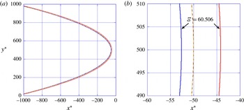
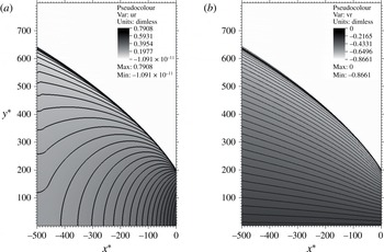
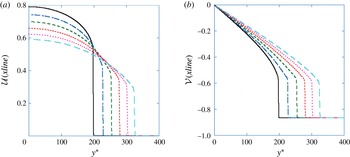
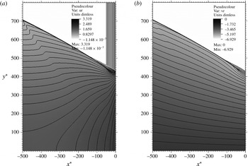
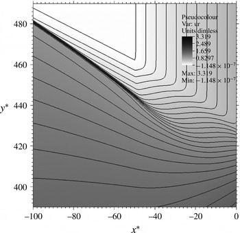
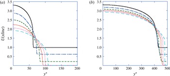
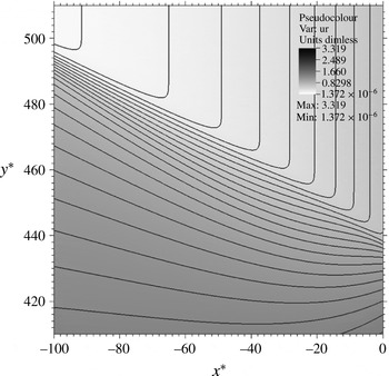
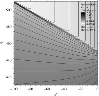
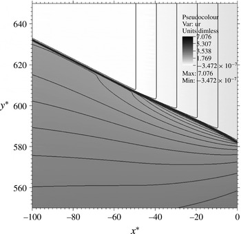
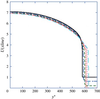
1 Introduction
Detonations can be thought of as self-sustaining shock waves. Many of the tools, both experimental and theoretical, that are used to study shock waves can also be applied to study detonations. In this paper, we develop a theory for the glancing oblique interaction of a planar detonation in a condensed-phase explosive with a rigid wall.
In detonation, the passage of a shock wave over the explosive triggers the heat-releasing reactions that in turn support the shock. A shock in a non-reactive material relies on some agent, referred to as a piston, to drive the subsonic flow that supports the shock. The energy release in an explosive provides local support for the detonation shock. Owing to the flow being exactly sonic in the shock frame at the point of reaction completion, the detonation is self-supporting. To this day, two basic models are used to describe detonation: (1) the Chapman–Jouguet (CJ) model and (2) the Zeldovich–von Neumann–Dø̈ring (ZND) model. The detonation shock initiates reaction in both models. For the CJ model, the length of the reaction zone supporting the detonation shock is so short that it is assumed to be indistinguishable from the shock rise time. The CJ model description is used when viewing detonation on a scale of hundreds of reaction-zone lengths, in an explosive that is similarly large, and when the details of what occurs on the scale of the reaction zone have little effect on detonation propagation. The speed of a self-sustaining detonation, the CJ detonation speed,
 $D_{CJ}$
, can be computed knowing only the overall detonation heat release and the equation of state (EOS) of the reaction products. The ZND model description is used when we are interested in more of the details of detonation, on a scale of tens of reaction-zone lengths. Although the reaction is initiated by the shock, reaction needs a finite time to complete. Effects dependent on the reaction-zone scale, such as the slowing and extinction of detonation that occur in smaller-size explosive charges, are intimately tied to the dynamics in the reaction zone. As with shocks in non-reactive materials, detonations can be supported by a piston that is sufficiently powerful so as to overdrive the flow to subsonic at the end of the reaction zone. This leads to a detonation speed,
 $D_{n}$
, for which
 $D_{n}>D_{CJ}$
. We use the parameter
 $f=D_{n}^{2}/D_{CJ}^{2}\geqslant 1$
to measure the degree of overdrive. A detonation experiencing Mach reflection is an overdriven detonation.
In this paper, we consider a small resolved heat-release (SRHR) detonation that becomes weakly overdriven by its glancing oblique interaction with a rigid wall. An SRHR explosive is a model for a condensed-phase high-energy explosive for which only a small fraction of the total detonation energy is released via a resolved chemical reaction. Our objective is twofold: (1) to understand the structure of the fully instantaneous reaction CJ detonation Mach reflection and (2) then to learn how the presence of a resolved chemical reaction zone influences the Mach reflection. Here, we restrict our attention to the problem of weak Mach reflection, generated by the glancing incidence of a one-dimensional detonation, supported at the CJ state with a rigid straight wall. In this limit and for both of these models, the flow in and following the reaction zone is weakly transonic, and our analysis will show that the flow is governed by the two-dimensional unsteady transonic small-disturbance theory (UTSD). We use a lead-shock-attached coordinate frame to derive the UTSD equations, and numerically solve the equations using a mixed method that is implicit in the transverse flow direction and explicit in the detonation propagation direction. For our SRHR model development, we limit consideration to state-independent reaction rates and weakly state-dependent reaction rates. To the best of our knowledge, the work presented here is the first complete and consistent theory for the fundamental and generic problem of the glancing oblique attack of a CJ detonation on a planar rigid surface.
The problem of Mach reflection of detonation is not a new one, having been extensively studied for gas detonation (see Ong Reference Ong1955; Meltzer et al.
Reference Meltzer, Shepherd, Akbar and Sabet1993; Shepherd, Schultz & Akbar Reference Shepherd, Schultz, Akbar, Ball, Hillier and Roberts1999), but has received only little attention for condensed-phase explosives (see Fowles & Isbell (Reference Fowles and Isbell1965), Lambourn & Wright (Reference Lambourn, Wright and Jacobs1965) and the recent numerical study of Bdzil, Short & Quirk (Reference Bdzil, Short, Quirk, Carney and Maienschein2015)). We begin our initial discussion by considering a scale-free self-supporting CJ detonation. In the reference frame attached to the detonation and moving with the detonation, and normal to the shock at speed
 $D_{CJ}$
, the flow downstream of the detonation is locally sonic.
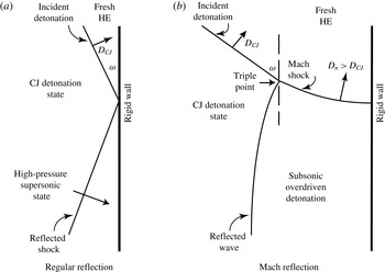
In the reference frame defined by the intersection of the propagating incident detonation and the rigid wall (see figure 1), the flow immediately downstream of the incident shock and near the wall is supersonic, becoming sonic only when the incident detonation and the wall are normal to one another (i.e.
 $\unicode[STIX]{x1D714}=90^{\circ }$
, where
 $\unicode[STIX]{x1D714}$
is the angle between the incident detonation and the wall). The reflection of the oblique incident detonation off of the rigid wall redirects some detonation energy downstream via a reflected shock over an approximately wedge-shaped region near the wall. This disturbs the flow downstream of the incident detonation and near the wall. When
 $\unicode[STIX]{x1D714}$
is sufficiently small (see figure 1
a), the incident detonation remains undisturbed at its intersection with the wall. However, as
 $\unicode[STIX]{x1D714}$
is increased, a reflected shock can no longer adequately turn the flow. Now, the reflected energy can propagate both upstream and away from the wall, which disturbs the incident detonation. This leaves in its wake a Mach shock (Mach stem) supported by an overdriven detonation, with pressure, etc. increased over the CJ detonation values, and a flow that is subsonic behind the lead Mach shock (see figure 1
b).
Two cases of the oblique interaction of a supported CJ detonation with a rigid wall. (a) The wave reflection problem for small values of
 $\unicode[STIX]{x1D714}$
, the angle between the incident detonation and the wall. For this case, the incident detonation remains undisturbed, with
 $D_{n}=D_{CJ}$
. (b) The wave reflection problem for moderate to large values of
 $\unicode[STIX]{x1D714}$
. For this case, the incident wave is disturbed by the interaction, where a Mach stem detonation shock, with
 $D_{n}>D_{CJ}$
, is required to turn the flow such that at the rigid wall the streamline remains parallel to the wall.

The standard approach for studying the reflection of an incident detonation off of an adjacent material interface is to use shock-polar theory (see Hornung (Reference Horning1986), Bdzil & Stewart (Reference Bdzil, Stewart and Zhang2012) and references therein). Shock-polar theory constructs a local scale-free solution at the point where the incident detonation shock intersects the material interface. Simple two-dimensional Riemann solutions, consisting of incident shocks, reflected shocks, slip lines and reflected rarefactions (Prandtl–Meyer fans), are used to patch together such a local solution. Expressions are derived for the pressure,
 $P$
, versus the streamline turning angle,
 $\unicode[STIX]{x1D6E9}$
, measured in the moving reference frame of the intersection point, that describe the exit state from the interaction in the materials on the two sides of the interface. These expressions for
 $P(\unicode[STIX]{x1D6E9})$
for each material are then matched (continuity of pressure and streamline turning angle) across the interface, which then yields the local point solution.
For the purposes of this paper, it suffices to consider that the adjacent material (the non-explosive) is rigid and non-deformable, which then closes our matching problem with
 $\unicode[STIX]{x1D6E9}$
constant across the interaction (typically referenced to
 $\unicode[STIX]{x1D6E9}=0$
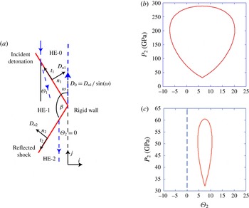
). Figure 2 displays a CJ detonation case for a condensed-phase explosive that is supported at the CJ state. The streamlines that are parallel to the interface in the quiescent unreacted explosive are turned towards the interface by the incident detonation shock. When the angle of the incident detonation shock,
 $\unicode[STIX]{x1D714}$
, is below a critical value then a reflected shock is generated in the detonation reaction products, where the included angle between the incident and reflected shock is
 $\unicode[STIX]{x1D6FD}$
. This shock turns the streamlines back parallel to the interface. With the state behind the incident wave and the angle between the incident wave and the interface prescribed, the shock polar for the explosive can be solved to get the exit state (pressure, streamline turning angle, etc.) generated by the interaction (see figure 2).
The solution for the oblique interaction of an instantaneous reaction, CJ detonation and a rigid material for regular reflection. The simple condensed-phase EOS model (see § 2) describes the detonation and the angle
 $\unicode[STIX]{x1D714}$
is prescribed (here
 $\unicode[STIX]{x1D714}=30^{\circ }$
). (a) The shock wave and streamline geometry. (b) The shock-polar diagram for the
 $\unicode[STIX]{x1D714}=30^{\circ }$
interaction. The solution state corresponds to
 $\unicode[STIX]{x1D6E9}_{2}=0$
. Of the two possible values of
 $P_{2}$
, the lower pressure corresponds to a supersonic flow in the frame of the moving interaction point, and it is the solution that corresponds to an undisturbed incident wave, which is of interest here. (c) The interaction for
 $\unicode[STIX]{x1D714}=60^{\circ }$
, when regular reflection is not possible and the shock polar does not intersect
 $\unicode[STIX]{x1D6E9}_{2}=0$
. The normal and tangent vectors to the shock are
 $n_{i}$
and
 $t_{i}$
, respectively, while
 $D_{ni}$
is the normal shock speed.

As the angle
 $\unicode[STIX]{x1D714}$
increases, the regular reflection solution, displayed in figure 2(b), is no longer possible as the reflected shock polar no longer intersects the
 $\unicode[STIX]{x1D6E9}=0$
line (see figure 2
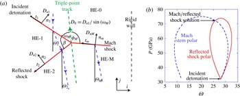
c). Then, the interaction point between the incident detonation and the reflected shock detaches from the interface and moves leftward into the explosive. Remaining in its wake, another incident detonation is formed (i.e. a Mach reflection), which in the simplest of cases spans between the interaction point and the material interface. The interaction point is referred to as the triple point: the point where the incident detonation, the reflected shock and the Mach detonation wave meet. To solve the interaction problem at the triple point, the track followed by the triple point (or, equivalently, the included angle between the incident detonation and the triple-point track,
 $\unicode[STIX]{x1D714}_{M}$
) must be known. Figure 3 displays the interaction at the triple point for a specified value of
 $\unicode[STIX]{x1D714}_{M}$
(
 $\unicode[STIX]{x1D714}_{M}=55^{\circ }$
).
The Mach reflection solution for an instantaneous reaction, CJ detonation. The angles displayed are measured relative to the triple-point track. The simple condensed-phase EOS model describes the detonating explosive; the angle
 $\unicode[STIX]{x1D714}_{M}$
is prescribed (
 $\unicode[STIX]{x1D714}_{M}=55^{\circ }$
). For this example,
 $\unicode[STIX]{x1D714}=75^{\circ }$
. (a) The shock wave and streamline geometry. (b) A shock-polar diagram for the ABS limit (see § 2) of the simple condensed-phase EOS model. The angle
 $\unicode[STIX]{x1D6E9}$
is measured relative to the tangent to the wall being zero. The included angles between the triple-point track and the incident and Mach shock are
 $\unicode[STIX]{x1D714}_{M}$
and
 $\unicode[STIX]{x1D719}_{M}$
, respectively.

In this paper, we will develop a theory for the track of the triple point and a solution for the entirety of the detonation Mach reflection problem for condensed-phase explosives, valid in the limit that the angle
 $\unicode[STIX]{x1D714}$
between the rigid wall and the incident detonation satisfies
 $(\unicode[STIX]{x03C0}/2-\unicode[STIX]{x1D714})\ll 1$
(the case of glancing incidence).
2 The simple condensed-phase EOS detonation model and shock-polar algebra
In our work, we adopt the simple constant adiabatic gamma EOS model description of condensed-phase high explosives (Fickett & Davis Reference Fickett and Davis1979; Bdzil Reference Bdzil1981; Wescott, Stewart & Bdzil Reference Wescott, Stewart and Bdzil2004; Short et al. Reference Short, Anguelova, Aslam, Bdzil, Henrick and Sharpe2008). This condensed-phase EOS model thermodynamics is given by
 $$\begin{eqnarray}E(P,\unicode[STIX]{x1D70C})=\frac{P}{(\unicode[STIX]{x1D6FE}-1)\unicode[STIX]{x1D70C}}-q\unicode[STIX]{x1D706},\end{eqnarray}$$
where
 $E(P,\unicode[STIX]{x1D70C})$
is the specific internal energy,
 $P$
is the pressure,
 $\unicode[STIX]{x1D70C}$
is the density,
 $\unicode[STIX]{x1D6FE}$
is the constant adiabatic gamma,
 $q$
is the specific energy release of the explosive and
 $\unicode[STIX]{x1D706}$
is the mass fraction of reacted explosive. For condensed-phase explosives, the adiabatic gamma is taken to be
 $\unicode[STIX]{x1D6FE}=3$
, the initial density of the unreacted explosive is
 $\unicode[STIX]{x1D70C}_{0}=2~\text{g}~\text{cm}^{-3}$
and the CJ detonation velocity is
 $D_{CJ}=8~\text{mm}~\unicode[STIX]{x03BC}\text{s}^{-1}$
. The CJ density, laboratory-frame particle velocity, pressure and sound speed are then
 $$\begin{eqnarray}\unicode[STIX]{x1D70C}_{CJ}=\frac{\unicode[STIX]{x1D6FE}+1}{\unicode[STIX]{x1D6FE}}\unicode[STIX]{x1D70C}_{0},\quad U_{CJ}=\frac{D_{CJ}}{\unicode[STIX]{x1D6FE}+1},\quad P_{CJ}=\frac{\unicode[STIX]{x1D70C}_{0}D_{CJ}^{2}}{\unicode[STIX]{x1D6FE}+1}\quad \text{and}\quad c_{CJ}=\frac{\unicode[STIX]{x1D6FE}D_{CJ}}{\unicode[STIX]{x1D6FE}+1}.\end{eqnarray}$$
The initial pressure,
 $P_{0}$
, in the unshocked unreacted explosive is set to zero, since the detonation pressure for condensed-phase detonation is many orders of magnitude greater than
 $P_{0}$
. Therefore, for this condensed-phase EOS model, the corresponding sound speed
 $c_{0}=0$
. The CJ Mach number,
 $M_{j}$
, and
 $q$
are then given by
 $$\begin{eqnarray}M_{j}=\frac{D_{CJ}}{\sqrt{\unicode[STIX]{x1D6FE}P_{0}/\unicode[STIX]{x1D70C}_{0}}}\rightarrow \infty \quad \text{and}\quad q=\frac{D_{CJ}^{2}}{2(\unicode[STIX]{x1D6FE}^{2}-1)}.\end{eqnarray}$$
With these parameters and limiting values, this condensed-phase EOS model is referred to as the ABS model (Aslam, Bdzil & Stewart Reference Aslam, Bdzil and Stewart1996). It provides a leading-order description of detonation in condensed-phase explosives.
For the problem of an incident CJ detonation interacting with a rigid wall considered here, we can compose a local solution by using only incident and reflected shocks. The shock polars are obtained from the shock jump conditions for mass, momentum in the shock normal direction and total energy, along with the continuity of the tangential velocity component. For this condensed-phase EOS model, the conditions for both the incident and the possible Mach stem detonation shock are parameterized by the normal detonation speed,
 $D_{CJ}$
, and the overdrive factor,
 $f$
,
 $$\begin{eqnarray}P_{1}=\frac{f\unicode[STIX]{x1D70C}_{0}D_{CJ}^{2}}{\unicode[STIX]{x1D6FE}+1}\left(1+\sqrt{1-1/f}\right)\quad \text{and}\quad \tan \unicode[STIX]{x1D6E9}_{1}=\frac{-P_{1}\cos \unicode[STIX]{x1D719}_{1}}{(\unicode[STIX]{x1D70C}_{0}D_{0}^{2}-P_{1})\sin \unicode[STIX]{x1D719}_{1}},\end{eqnarray}$$
where the detonation overdrive factor is
 $$\begin{eqnarray}f=\frac{D_{nI}^{2}}{D_{CJ}^{2}},\end{eqnarray}$$
with
 $D_{nI}=D_{n1}=D_{CJ}$
for the incident detonation and
 $D_{nI}=D_{nM}$
for the possible Mach stem detonation. Here,
 $D_{0}$
is the phase velocity of the incident detonation along either the rigid wall or the triple-point track, whichever is relevant,
 $$\begin{eqnarray}D_{0}=\frac{D_{CJ}}{\sin \unicode[STIX]{x1D714}_{1}}=\frac{D_{nI}}{\sin \unicode[STIX]{x1D719}_{1}},\end{eqnarray}$$
where
 $\unicode[STIX]{x1D719}_{1}=\unicode[STIX]{x03C0}-\unicode[STIX]{x1D714}$
for the incident wave and
 $\unicode[STIX]{x1D719}_{1}=\unicode[STIX]{x1D719}_{M}$
for the Mach stem, and where
 $\unicode[STIX]{x1D6E9}_{1}$
is the streamline turning angle measured relative to the rigid wall (see figures 2
a and 3
a for the definition of variables). For Mach stems, the allowable range for
 $\unicode[STIX]{x1D719}_{M}$
is
 $$\begin{eqnarray}\unicode[STIX]{x1D714}_{M}\leqslant \unicode[STIX]{x1D719}_{M}\leqslant \unicode[STIX]{x03C0}-\unicode[STIX]{x1D714}_{M}.\end{eqnarray}$$
The conditions behind the reflected shock, labelled as shock 2, are parameterized by the state behind the incident CJ detonation shock,
 $$\begin{eqnarray}\frac{\unicode[STIX]{x1D70C}_{0}}{\unicode[STIX]{x1D70C}_{1}}=\frac{\unicode[STIX]{x1D6FE}}{\unicode[STIX]{x1D6FE}+1},\quad \boldsymbol{n}_{1}\boldsymbol{\cdot }\boldsymbol{U}_{lab1}=\frac{D_{n1}}{\unicode[STIX]{x1D6FE}+1},\quad P_{1}=\frac{\unicode[STIX]{x1D70C}_{0}D_{n1}^{2}}{\unicode[STIX]{x1D6FE}+1},\end{eqnarray}$$
with
 $D_{n1}=D_{CJ}$
, the included angle between the incident detonation and the rigid wall
 $\unicode[STIX]{x1D714}$
, and the included angle
 $\unicode[STIX]{x1D6FD}$
between the incident and reflected shocks (see figures 2
a and 3
a), where
 $$\begin{eqnarray}0\leqslant \unicode[STIX]{x1D6FD}\leqslant \frac{\unicode[STIX]{x03C0}}{2}\left(1+\text{sign}\left(\cot ^{2}\unicode[STIX]{x1D714}-\left(\frac{\unicode[STIX]{x1D6FE}}{\unicode[STIX]{x1D6FE}+1}\right)^{2}\right)\right)+\arctan \left(\frac{-{\displaystyle \frac{2\unicode[STIX]{x1D6FE}}{\unicode[STIX]{x1D6FE}+1}}\cot \unicode[STIX]{x1D714}}{\cot ^{2}\unicode[STIX]{x1D714}-\left({\displaystyle \frac{\unicode[STIX]{x1D6FE}}{\unicode[STIX]{x1D6FE}+1}}\right)^{2}}\right)\end{eqnarray}$$
gives the range for
 $\unicode[STIX]{x1D6FD}$
that moves one completely around the reflected shock polar for the case of CJ detonation (Bdzil & Stewart Reference Bdzil, Stewart and Zhang2012). The pressure behind the reflected shock, given as a function of
 $\unicode[STIX]{x1D6FD}$
and
 $\unicode[STIX]{x1D714}$
, is
 $$\begin{eqnarray}P_{2}=P_{1}+\frac{2\unicode[STIX]{x1D70C}_{1}}{\unicode[STIX]{x1D6FE}+1}\left[(\boldsymbol{n}_{I}\boldsymbol{\cdot }\boldsymbol{n}_{2}(\boldsymbol{n}_{I}\boldsymbol{\cdot }\boldsymbol{U}_{lab1})-D_{n2})^{2}-\frac{\unicode[STIX]{x1D6FE}P_{1}}{\unicode[STIX]{x1D70C}_{1}}\right],\end{eqnarray}$$
with
 $$\begin{eqnarray}(\boldsymbol{n}_{I}\boldsymbol{\cdot }\boldsymbol{n}_{2}(\boldsymbol{n}_{I}\boldsymbol{\cdot }\boldsymbol{U}_{lab1})-D_{n2})=D_{n1}\left(\frac{\cos \unicode[STIX]{x1D6FD}}{\unicode[STIX]{x1D6FE}+1}-\frac{\sin (\unicode[STIX]{x1D714}+\unicode[STIX]{x1D6FD})}{\sin \unicode[STIX]{x1D714}}\right).\end{eqnarray}$$
The streamline turning angle behind the reflected shock,
 $\unicode[STIX]{x1D6E9}_{2}$
, is given by
 $$\begin{eqnarray}\tan \unicode[STIX]{x1D6E9}_{2}=\frac{U_{lab2x}}{D_{0}-U_{lab2y}},\end{eqnarray}$$
where
 $$\begin{eqnarray}\displaystyle & \displaystyle U_{lab2x}=(\boldsymbol{n}_{2}\boldsymbol{\cdot }\boldsymbol{U}_{lab2})\cos (\unicode[STIX]{x1D6FD}+\unicode[STIX]{x1D714})-(\boldsymbol{t}_{2}\boldsymbol{\cdot }\boldsymbol{U}_{lab2})\sin (\unicode[STIX]{x1D6FD}+\unicode[STIX]{x1D714}), & \displaystyle\end{eqnarray}$$
 $$\begin{eqnarray}\displaystyle & \displaystyle U_{lab2y}=(\boldsymbol{n}_{2}\boldsymbol{\cdot }\boldsymbol{U}_{lab2})\sin (\unicode[STIX]{x1D6FD}+\unicode[STIX]{x1D714})+(\boldsymbol{t}_{2}\boldsymbol{\cdot }\boldsymbol{U}_{lab2})\cos (\unicode[STIX]{x1D6FD}+\unicode[STIX]{x1D714}), & \displaystyle\end{eqnarray}$$
with
 $$\begin{eqnarray}\displaystyle \boldsymbol{n}_{2}\boldsymbol{\cdot }\boldsymbol{U}_{lab2} & = & \displaystyle D_{n2}+\left(\frac{\unicode[STIX]{x1D6FE}-1}{\unicode[STIX]{x1D6FE}+1}\right)(\boldsymbol{n}_{I}\boldsymbol{\cdot }\boldsymbol{n}_{2}(\boldsymbol{n}_{I}\boldsymbol{\cdot }\boldsymbol{U}_{lab1})-D_{n2})\nonumber\\ \displaystyle & & \displaystyle +\,\frac{2}{\unicode[STIX]{x1D6FE}+1}\left(\frac{\unicode[STIX]{x1D6FE}D_{n1}}{\unicode[STIX]{x1D6FE}+1}\right)^{2}\frac{1}{(\boldsymbol{n}_{I}\boldsymbol{\cdot }\boldsymbol{n}_{2}(\boldsymbol{n}_{I}\boldsymbol{\cdot }\boldsymbol{U}_{lab1})-D_{n2})},\end{eqnarray}$$
 $$\begin{eqnarray}\displaystyle & \displaystyle \boldsymbol{t}_{2}\boldsymbol{\cdot }\boldsymbol{U}_{lab2}=-\frac{D_{n1}}{\unicode[STIX]{x1D6FE}+1}\sin (\unicode[STIX]{x1D6FD}), & \displaystyle\end{eqnarray}$$
 $$\begin{eqnarray}\displaystyle & \displaystyle D_{n2}=D_{0}\sin (\unicode[STIX]{x1D714}+\unicode[STIX]{x1D6FD}). & \displaystyle\end{eqnarray}$$
With the auxiliary functions, (2.11) and (2.13)–(2.17), being only functions of
 $\unicode[STIX]{x1D6FD}$
and
 $\unicode[STIX]{x1D714}$
that are defined by these equations, scanning
 $\unicode[STIX]{x1D6FD}$
over the range given in (2.9) for (2.10) and (2.12) gives the shock polar for the reflected shock,
 $P_{2}(\unicode[STIX]{x1D6E9})$
. This corresponds to the flow exiting from the reflected shock.
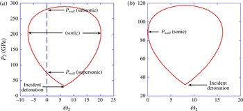
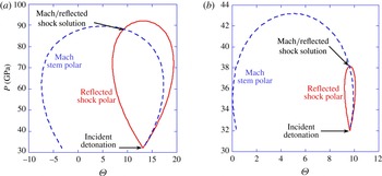
In figure 4, we show for the ABS model two examples of the constraints placed by the shock-polar analysis on the point solution at the intersection of the incident CJ detonation with the rigid wall, including the reflected shock that is generated. For the ABS model shock polars, the portion of the
 $P(\unicode[STIX]{x1D6E9})$
polars below (above) the vertical tangency point on the polar corresponds to a supersonic (subsonic) flow when measured in the reference frame of the polar. In all cases, the lowest pressure corresponds to the CJ pressure of the incident detonation (
 $P_{CJ}=32~\text{GPa}$
), while the minimum pressure point on the polar corresponds to the streamline turning angle behind the incident detonation, measured with respect to the rigid wall (positive angles correspond to a flow into the wall).
The
 $P_{2}(\unicode[STIX]{x1D6E9}_{2})$
shock polars for the ABS model. Regular reflection for
 $\unicode[STIX]{x1D714}=30^{\circ }$
is displayed in (a). Regular reflection with the wall is lost at
 $\unicode[STIX]{x1D714}=45^{\circ }$
(see b), with some form of irregular reflection required for
 $\unicode[STIX]{x1D714}>45^{\circ }$
. The streamline turning angle is measured relative to the tangent to the rigid wall being zero. The incident detonation state and the match pressure into the wall are marked for both the
 $\unicode[STIX]{x1D714}=30^{\circ }$
and
 $\unicode[STIX]{x1D714}=45^{\circ }$
cases.

For
 $0\leqslant \unicode[STIX]{x1D714}\leqslant 45^{\circ }$
, regular shock reflection is observed for the ABS model with the interaction point riding along the rigid wall, where the streamline turning angle is zero. The shock polar for
 $\unicode[STIX]{x1D714}=30^{\circ }$
is displayed in figure 4(a). The zero turning angle supersonic flow pressure of
 $\simeq 70~\text{GPa}$
is what is stable and observed. The solutions for other values of
 $\unicode[STIX]{x1D714}$
, in the range of
 $0^{\circ }<\unicode[STIX]{x1D714}<45^{\circ }$
, look similar to those for
 $\unicode[STIX]{x1D714}=30^{\circ }$
. As
 $\unicode[STIX]{x1D714}$
increases towards
 $\unicode[STIX]{x1D714}=45^{\circ }$
, the pressure is observed to vary somewhat around a nominal value of
 $\simeq 70~\text{GPa}$
, finally reaching a value of
 $\simeq 90~\text{GPa}$
for
 $\unicode[STIX]{x1D714}=45^{\circ }$
. The shock polar for
 $\unicode[STIX]{x1D714}=45^{\circ }$
is displayed in figure 4(b). Thus, for the ABS model CJ detonation, we find regular shock reflection for
 $0\leqslant \unicode[STIX]{x1D714}\leqslant 45^{\circ }$
and expect shock-polar theory to predict the reflected state pressure, etc.
Two cases of Mach reflection for the ABS model. The Mach reflection polar for
 $\unicode[STIX]{x1D714}=55^{\circ }$
and
 $\unicode[STIX]{x1D714}_{M}=50^{\circ }$
is displayed in (a) and that for
 $\unicode[STIX]{x1D714}=80^{\circ }$
with
 $\unicode[STIX]{x1D714}_{M}=75^{\circ }$
is displayed in (b). The available Mach reflection pressure drops as
 $\unicode[STIX]{x1D714}$
increases past
 $\unicode[STIX]{x1D714}=45^{\circ }$
, with the Mach reflection pressure approaching
 $P_{CJ}=32~\text{GPa}$
as
 $\unicode[STIX]{x1D714}\rightarrow 90^{\circ }$
.

When
 $\unicode[STIX]{x1D714}>45^{\circ }$
, regular reflection is no longer possible for the ABS limit CJ detonation model, as the reflected shock polar pulls away from
 $\unicode[STIX]{x1D6E9}_{2}=0$
. Now, a Mach reflection state is proposed, as described in figure 5(a,b). The cases of Mach reflection for
 $\unicode[STIX]{x1D714}=55^{\circ }$
with
 $\unicode[STIX]{x1D714}_{M}=50^{\circ }$
and
 $\unicode[STIX]{x1D714}=80^{\circ }$
with
 $\unicode[STIX]{x1D714}_{M}=75^{\circ }$
are displayed in figures 5(a) and 5(b) respectively. In these cases, the interaction point (triple point), which is the confluence of the incident detonation (1), the reflected shock (2) and the overdriven detonation Mach shock (M), tracks along a line that makes an angle
 $\unicode[STIX]{x1D714}-\unicode[STIX]{x1D714}_{M}$
with the wall. The value of
 $\unicode[STIX]{x1D714}_{M}$
, with
 $\unicode[STIX]{x1D714}_{M}\leqslant \unicode[STIX]{x1D714}$
, is not determined by shock-polar theory. The diagrams in figure 5(a,b) represent only possible solutions for an imposed choice of
 $\unicode[STIX]{x1D714}_{M}$
. The pressure and streamline turning angle at the triple point are given by the point in these figures labelled as ‘Mach/reflected shock solution’. As is evident from these figures, the Mach stem pressure varies substantially with changes in
 $\unicode[STIX]{x1D714}$
. Since the track followed by the triple point as it leaves the wall is a required input and is not given by shock-polar theory, the polar theory is unable to provide us with much guidance as to the Mach reflection state. At best, all that can be said is that shock-polar theory provides a constraint as to what is possible, but not the solution.
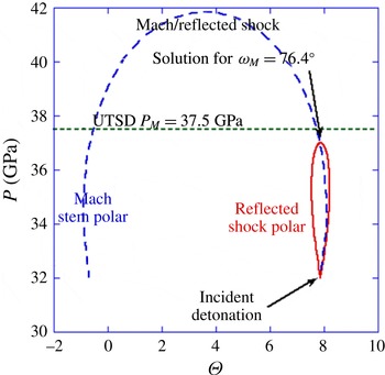
Figure 5(b) displays the shock-polar diagram for a case of glancing incidence of the detonation with the wall, with
 $\unicode[STIX]{x1D714}=80^{\circ }$
and
 $\unicode[STIX]{x1D714}_{M}$
assumed as
 $\unicode[STIX]{x1D714}_{M}=75^{\circ }$
. In this case, the Mach reflection pressure is only slightly greater than the CJ detonation pressure. In the next section, we describe a detailed model for Mach reflection of a CJ detonation that applies when
 $\unicode[STIX]{x03C0}/2-\unicode[STIX]{x1D714}\ll 1$
, the case of glancing incidence. The fundamental CJ detonation model helps us to understand the differences between inert material and detonation Mach reflection. In neglecting the details of the reaction zone, the CJ detonation provides a picture of Mach reflection when detonation is viewed on a scale much larger than the reaction-zone thickness scale.
3 Chapman–Jouguet detonation Mach reflection at glancing incidence
The locally convergent flow generated near the wall leads to Mach reflection, with the incident instantaneous reaction CJ detonation becoming overdriven in that region. In the limit of glancing incidence,
 $\unicode[STIX]{x03C0}/2-\unicode[STIX]{x1D714}\ll 1$
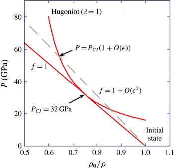
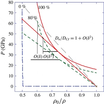
, the degree of overdrive is weak (see figure 6). Here, and for this case, we develop a solution strategy for solving the problem of irregular detonation reflection (Mach reflection).
The
 $P$
versus
 $(\unicode[STIX]{x1D70C}_{0}/\unicode[STIX]{x1D70C})$
diagram (referred to as the PV diagram) for an instantaneous reaction detonation for the ABS model. Here,
 $f=(D_{n}/D_{CJ})^{2}$
is the detonation overdrive, with
 $f>1$
corresponding to an overdriven detonation.

We begin our discussion by setting down a simple Hugoniot diagram for an instantaneous reaction detonation (see Fickett & Davis Reference Fickett and Davis1979; Fickett Reference Fickett1985). Figure 6 displays the standard PV diagram for an instantaneous reaction detonation. The curve represents the pressure–volume (PV) states that are consistent with the conservation of energy and mass (Hugoniot), while the straight lines are states consistent with conservation of momentum and mass (Rayleigh line). Both of these expressions are parameterized by
 $D_{n}$
. The slowest possible detonation travels at
 $D_{n}=D_{CJ}$
, the Chapman–Jouguet speed. The parameter
 $f=(D_{n}/D_{CJ})^{2}$
is the overdrive factor, where
 $f>1$
describes a detonation moving faster than
 $D_{CJ}$
. In the reference frame of the detonation shock, the flow is exactly sonic for the CJ detonation. Increases in the detonation speed,
 $D_{n}/D_{CJ}=1+O(\unicode[STIX]{x1D716}^{2})$
, with
 $\unicode[STIX]{x1D716}^{2}\ll 1$
, produce changes in the detonation pressure (and of other detonation-state variables) of order
 $P/P_{CJ}=1+O(\unicode[STIX]{x1D716})$
. This difference in sensitivity of
 $D_{n}$
compared with
 $P$
on
 $\unicode[STIX]{x1D716}$
allows the changes in the flow (which are
 $O(\unicode[STIX]{x1D716})$
for a weakly overdriven detonation) to decouple from the changes in detonation speed produced by the flow (which are
 $O(\unicode[STIX]{x1D716}^{2})$
). The expressions for the Hugoniot curve and the Rayleigh line for our condensed-phase EOS model are parameterized by
 $D_{n}$
, and are given by
 $$\begin{eqnarray}\displaystyle & \displaystyle \left(1-\frac{\unicode[STIX]{x1D70C}_{0}^{2}}{\unicode[STIX]{x1D70C}_{1}^{2}}\right)\frac{D_{n}^{2}}{2}-\frac{\unicode[STIX]{x1D6FE}}{\unicode[STIX]{x1D6FE}+1}\frac{P_{1}}{\unicode[STIX]{x1D70C}_{0}}\frac{\unicode[STIX]{x1D70C}_{0}}{\unicode[STIX]{x1D70C}_{1}}+\frac{D_{CJ}^{2}}{2(\unicode[STIX]{x1D6FE}^{2}-1)}=0, & \displaystyle\end{eqnarray}$$
 $$\begin{eqnarray}\displaystyle & \displaystyle \frac{P_{1}}{\unicode[STIX]{x1D70C}_{0}}=\left(1-\frac{\unicode[STIX]{x1D70C}_{0}}{\unicode[STIX]{x1D70C}_{1}}\right)D_{n}^{2}. & \displaystyle\end{eqnarray}$$
Elimination of
 $\unicode[STIX]{x1D70C}_{0}/\unicode[STIX]{x1D70C}_{1}$
between (3.1) and (3.2) returns two possible detonation states, an overdriven strong detonation and a supersonic weak detonation given by
 $$\begin{eqnarray}P=P_{CJ}f\left(1\pm \sqrt{1-\frac{1}{f}}\right),\end{eqnarray}$$
with
 $$\begin{eqnarray}f=\frac{D_{n}^{2}}{D_{CJ}^{2}}=1+\unicode[STIX]{x1D716}^{2}.\end{eqnarray}$$
Thus,
 $$\begin{eqnarray}\displaystyle \left.\begin{array}{@{}c@{}}P=P_{CJ}\left(1+\unicode[STIX]{x1D716}^{2}\pm \unicode[STIX]{x1D716}\sqrt{1+\unicode[STIX]{x1D716}^{2}}\right),\\ P=P_{CJ}(1\pm \unicode[STIX]{x1D716}+O(\unicode[STIX]{x1D716}^{2})).\end{array}\right\} & & \displaystyle\end{eqnarray}$$
The state
 $P=P_{CJ}(1+\unicode[STIX]{x1D716}+O(\unicode[STIX]{x1D716}^{2}))$
is the overdriven state of interest in our analysis and complies with the order estimates given above. With
 $\unicode[STIX]{x1D716}^{2}\ll 1$
, this sets the form of our perturbation expansion off the CJ state (at least for a subset of the flow variables) in our analysis of the flow supporting detonation Mach reflection.
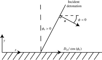
The support for detonation Mach reflection comes from the transverse flow generated by the interaction of an oblique CJ detonation shock with a rigid horizontal wall. Figure 7 displays the initial state of the flow we consider. The state to the right of the CJ detonation is quiescent, with the initial density
 $\unicode[STIX]{x1D70C}_{0}$
and the pressure
 $P_{0}=0$
. The state to the left of the detonation is the CJ state for our condensed-phase EOS model (given by (2.8)), where the
 $x$
- and
 $y$
-components of the particle velocity are
 $$\begin{eqnarray}U_{labx}^{0}=U_{CJ}\cos \unicode[STIX]{x1D719}_{e}\quad \text{and}\quad U_{laby}^{0}=-U_{CJ}\sin \unicode[STIX]{x1D719}_{e}.\end{eqnarray}$$
In our analysis, we consider that
 $\unicode[STIX]{x1D719}_{e}\ll 1$
is a second small parameter, selected so as to ensure that
 $\unicode[STIX]{x1D716}^{2}$
, the amount of overdrive, is maintained at small values. Since
 $\unicode[STIX]{x1D719}_{e}=\unicode[STIX]{x03C0}/2-\unicode[STIX]{x1D714}\ll 1$
, the initial transverse velocity,
 $U_{laby}^{0}$
, is small. The exact relationship between
 $\unicode[STIX]{x1D716}^{2}$
and
 $\unicode[STIX]{x1D719}_{e}$
will be set so as to cause the strongest possible interaction between these two parameters.
The initial configuration for the collision of a CJ detonation with a rigid floor. In our analysis, we will assume that the angle
 $\unicode[STIX]{x1D719}_{e}=\unicode[STIX]{x03C0}/2-\unicode[STIX]{x1D714}\ll 1$
(the case of glancing incidence). The initial configuration of the detonation front is
 $x_{s0}=(D_{CJ}/\cos \unicode[STIX]{x1D719}_{e})t+y\tan \unicode[STIX]{x1D719}_{e}$
. The angle
 $\unicode[STIX]{x1D719}<0$
measures the local angle between the evolving detonation shock and the
 $x$
-axis.

4 Distinguished scales analysis for
 $\unicode[STIX]{x1D716}^{2}\ll 1$
and
$\unicode[STIX]{x1D719}_{e}\ll 1$


Here, we give the problem formulation. The two-dimensional slab-geometry time-dependent dimensional Euler equations are used to describe the flow. The conservation equations of mass, momentum and energy are
 $$\begin{eqnarray}\displaystyle & \displaystyle (\dot{\unicode[STIX]{x1D70C}})+\unicode[STIX]{x1D70C}\unicode[STIX]{x1D735}\boldsymbol{\cdot }\boldsymbol{U}_{lab}=0, & \displaystyle\end{eqnarray}$$
 $$\begin{eqnarray}\displaystyle & \displaystyle \unicode[STIX]{x1D70C}(\dot{\boldsymbol{U}}_{lab})+\unicode[STIX]{x1D735}P=0, & \displaystyle\end{eqnarray}$$
 $$\begin{eqnarray}\displaystyle & \displaystyle ({\dot{E}})+\left(\dot{\frac{1}{\unicode[STIX]{x1D70C}}}\right)P=0, & \displaystyle\end{eqnarray}$$
where
 $(\dot{\;\;})$
is the substantial derivative,
 $$\begin{eqnarray}(\dot{\;\;})=\frac{\unicode[STIX]{x2202}}{\unicode[STIX]{x2202}t}+\boldsymbol{U}_{lab}\boldsymbol{\cdot }\unicode[STIX]{x1D735},\end{eqnarray}$$
 $E(P,\unicode[STIX]{x1D70C})$
is the specific internal energy of the detonation products and
 $\boldsymbol{U}_{lab}$
is the vector particle velocity measured in our stationary laboratory reference frame (see figure 7). By expanding the notation into the
 $x,y$
-Cartesian reference frame displayed in figure 7, rewriting the energy equation into a form more convenient for our analysis (called the master equation (Bdzil & Stewart Reference Bdzil, Stewart and Zhang2012)) and introducing a subsidiary equation for the flow vorticity, we have
 $$\begin{eqnarray}\displaystyle & \displaystyle \frac{\unicode[STIX]{x2202}\unicode[STIX]{x1D70C}}{\unicode[STIX]{x2202}t}+\unicode[STIX]{x1D735}\boldsymbol{\cdot }(\unicode[STIX]{x1D70C}\boldsymbol{U}_{lab})=0, & \displaystyle\end{eqnarray}$$
 $$\begin{eqnarray}\displaystyle & \displaystyle \frac{\unicode[STIX]{x2202}\boldsymbol{U}_{lab}}{\unicode[STIX]{x2202}t}+\boldsymbol{U}_{lab}\boldsymbol{\cdot }\unicode[STIX]{x1D735}(\boldsymbol{U}_{lab})+\frac{1}{\unicode[STIX]{x1D70C}}\unicode[STIX]{x1D735}P=0, & \displaystyle\end{eqnarray}$$
 $$\begin{eqnarray}\displaystyle & \displaystyle \frac{1}{\unicode[STIX]{x1D70C}}\frac{\unicode[STIX]{x2202}P}{\unicode[STIX]{x2202}t}-\frac{\unicode[STIX]{x2202}\;}{\unicode[STIX]{x2202}t}\left(\frac{1}{2}\boldsymbol{U}_{lab}\boldsymbol{\cdot }\boldsymbol{U}_{lab}\right)-\boldsymbol{U}_{lab}\boldsymbol{\cdot }\unicode[STIX]{x1D735}\left(\frac{1}{2}\boldsymbol{U}_{lab}\boldsymbol{\cdot }\boldsymbol{U}_{lab}\right)+c^{2}\unicode[STIX]{x1D735}\boldsymbol{\cdot }\boldsymbol{U}_{lab}=0 & \displaystyle\end{eqnarray}$$
and
 $$\begin{eqnarray}\frac{\unicode[STIX]{x2202}\;}{\unicode[STIX]{x2202}t}\left(\frac{\unicode[STIX]{x1D6FA}}{\unicode[STIX]{x1D70C}}\right)+\boldsymbol{U}_{lab}\boldsymbol{\cdot }\unicode[STIX]{x1D735}\left(\frac{\unicode[STIX]{x1D6FA}}{\unicode[STIX]{x1D70C}}\right)=\frac{1}{\unicode[STIX]{x1D70C}}\left(\frac{\unicode[STIX]{x2202}\;}{\unicode[STIX]{x2202}y}\left(\frac{1}{\unicode[STIX]{x1D70C}}\right)\frac{\unicode[STIX]{x2202}P}{\unicode[STIX]{x2202}x}-\frac{\unicode[STIX]{x2202}\;}{\unicode[STIX]{x2202}x}\left(\frac{1}{\unicode[STIX]{x1D70C}}\right)\frac{\unicode[STIX]{x2202}P}{\unicode[STIX]{x2202}y}\right),\end{eqnarray}$$
where
 $c^{2}$
is the square of the frozen sound speed,
 $$\begin{eqnarray}c^{2}=(P/\unicode[STIX]{x1D70C}^{2}-E_{\unicode[STIX]{x1D70C}})/E_{P},\end{eqnarray}$$
and
 $\unicode[STIX]{x1D6FA}$
is the vorticity,
 $$\begin{eqnarray}\unicode[STIX]{x1D6FA}=\frac{\unicode[STIX]{x2202}U_{laby}}{\unicode[STIX]{x2202}x}-\frac{\unicode[STIX]{x2202}U_{labx}}{\unicode[STIX]{x2202}y}.\end{eqnarray}$$
Equations (4.5)–(4.6) are the mass and momentum equations respectively, while (4.7) is the master equation (an alternative form of the energy equation) and (4.8) is the vorticity equation. Subscripts on thermodynamic variables, such as
 $E(P,\unicode[STIX]{x1D70C})$
, denote partial derivatives with respect to the subscripted variable.
Initially, the flow is configured as shown in figure 7, where an oblique CJ detonation is moving into quiescent explosive, found to its right, and being supported by the CJ detonation state to its left. Given that for
 $\unicode[STIX]{x1D719}_{e}\ll 1$
the
 $y$
-component of velocity will be small, it is convenient to introduce a non-orthogonal shock-based reference frame, where the
 $y$
-direction coordinate remains unchanged and the new
 $x$
-direction coordinate is measured relative to the leading evolving detonation shock locus,
 $\unicode[STIX]{x1D713}_{s}$
, here given as
 $$\begin{eqnarray}\unicode[STIX]{x1D713}_{s}(y,t)=(D_{CJ}/\cos \unicode[STIX]{x1D719}_{e})t+y\tan \unicode[STIX]{x1D719}_{e}+\tilde{\unicode[STIX]{x1D713}}_{s}(y,t),\end{eqnarray}$$
where
 $\tilde{\unicode[STIX]{x1D713}}_{s}(y,t)$
represents the perturbation off the shock shape translated and unperturbed initial value,
 $x_{s0}=(D_{CJ}/\cos \unicode[STIX]{x1D719}_{e})t+y\tan \unicode[STIX]{x1D719}_{e}$
. With the shock-attached coordinates defined through
 $$\begin{eqnarray}\displaystyle & \tilde{x}=x-\unicode[STIX]{x1D713}_{s}(y,t), & \displaystyle\end{eqnarray}$$
 $$\begin{eqnarray}\displaystyle & {\tilde{y}}=y, & \displaystyle\end{eqnarray}$$
we have
 $$\begin{eqnarray}\displaystyle & \displaystyle \left(\frac{\unicode[STIX]{x2202}\;}{\unicode[STIX]{x2202}x}\right)_{y,t}=\left(\frac{\unicode[STIX]{x2202}\;}{\unicode[STIX]{x2202}\tilde{x}}\right)_{{\tilde{y}},t}, & \displaystyle\end{eqnarray}$$
 $$\begin{eqnarray}\displaystyle & \displaystyle \left(\frac{\unicode[STIX]{x2202}\;}{\unicode[STIX]{x2202}y}\right)_{x,t}=\left(\frac{\unicode[STIX]{x2202}\;}{\unicode[STIX]{x2202}{\tilde{y}}}\right)_{\tilde{x},t}-\left(\frac{\unicode[STIX]{x2202}\unicode[STIX]{x1D713}_{s}}{\unicode[STIX]{x2202}{\tilde{y}}}\right)_{t}\left(\frac{\unicode[STIX]{x2202}\;}{\unicode[STIX]{x2202}\tilde{x}}\right)_{{\tilde{y}},t}, & \displaystyle\end{eqnarray}$$
 $$\begin{eqnarray}\displaystyle & \displaystyle \left(\frac{\unicode[STIX]{x2202}\;}{\unicode[STIX]{x2202}t}\right)_{x,y}=\left(\frac{\unicode[STIX]{x2202}\;}{\unicode[STIX]{x2202}t}\right)_{\tilde{x},{\tilde{y}}}-\left(\frac{\unicode[STIX]{x2202}\unicode[STIX]{x1D713}_{s}}{\unicode[STIX]{x2202}t}\right)_{{\tilde{y}}}\left(\frac{\unicode[STIX]{x2202}\;}{\unicode[STIX]{x2202}\tilde{x}}\right)_{{\tilde{y}},t}. & \displaystyle\end{eqnarray}$$
Written in these shock-attached coordinates and introducing the transformed particle velocity (to maintain consistency with Bdzil & Stewart Reference Bdzil and Stewart1986)
 $$\begin{eqnarray}\tilde{\boldsymbol{u}}=\boldsymbol{U}_{lab}-\hat{i} (D_{CJ}/\cos \unicode[STIX]{x1D719}_{e})=\hat{i} (U_{labx}-D_{CJ}/\cos \unicode[STIX]{x1D719}_{e})+{\hat{j}}U_{laby},\end{eqnarray}$$
the Euler equations, (4.5)–(4.10), become after considerable algebra
 $$\begin{eqnarray}\displaystyle & \displaystyle {\tilde{N}}(\unicode[STIX]{x1D70C})+\tilde{\boldsymbol{u}}\boldsymbol{\cdot }\tilde{\boldsymbol{M}}(\unicode[STIX]{x1D70C})+\unicode[STIX]{x1D70C}\tilde{\boldsymbol{M}}\boldsymbol{\cdot }\tilde{\boldsymbol{u}}=0, & \displaystyle\end{eqnarray}$$
 $$\begin{eqnarray}\displaystyle & \displaystyle {\tilde{N}}(\tilde{\boldsymbol{u}})+\tilde{\boldsymbol{u}}\boldsymbol{\cdot }\tilde{\boldsymbol{M}}(\tilde{\boldsymbol{u}})+\frac{1}{\unicode[STIX]{x1D70C}}\tilde{\boldsymbol{M}}(P)=0, & \displaystyle\end{eqnarray}$$
 $$\begin{eqnarray}\displaystyle & \displaystyle \frac{1}{\unicode[STIX]{x1D70C}}{\tilde{N}}(P)-\frac{1}{2}{\tilde{N}}(\tilde{\boldsymbol{u}}\boldsymbol{\cdot }\tilde{\boldsymbol{u}})-\frac{1}{2}\tilde{\boldsymbol{u}}\boldsymbol{\cdot }\tilde{\boldsymbol{M}}(\tilde{\boldsymbol{u}}\boldsymbol{\cdot }\tilde{\boldsymbol{u}})+c^{2}\tilde{\boldsymbol{M}}\boldsymbol{\cdot }\tilde{\boldsymbol{u}}=0 & \displaystyle\end{eqnarray}$$
and
 $$\begin{eqnarray}{\tilde{N}}\left(\frac{\tilde{\unicode[STIX]{x1D6FA}}}{\unicode[STIX]{x1D70C}}\right)+\tilde{\boldsymbol{u}}\boldsymbol{\cdot }\tilde{\boldsymbol{M}}\left(\frac{\tilde{\unicode[STIX]{x1D6FA}}}{\unicode[STIX]{x1D70C}}\right)=\frac{1}{\unicode[STIX]{x1D70C}}\left(\frac{\unicode[STIX]{x2202}\;}{\unicode[STIX]{x2202}{\tilde{y}}}\left(\frac{1}{\unicode[STIX]{x1D70C}}\right)\frac{\unicode[STIX]{x2202}P}{\unicode[STIX]{x2202}\tilde{x}}-\frac{\unicode[STIX]{x2202}\;}{\unicode[STIX]{x2202}\tilde{x}}\left(\frac{1}{\unicode[STIX]{x1D70C}}\right)\frac{\unicode[STIX]{x2202}P}{\unicode[STIX]{x2202}{\tilde{y}}}\right),\end{eqnarray}$$
with
 $$\begin{eqnarray}\tilde{\unicode[STIX]{x1D6FA}}=\left(\frac{\unicode[STIX]{x2202}\tilde{u} _{y}}{\unicode[STIX]{x2202}\tilde{x}}\right)_{{\tilde{y}},t}-\left(\frac{\unicode[STIX]{x2202}\tilde{u} _{x}}{\unicode[STIX]{x2202}{\tilde{y}}}\right)_{\tilde{x},t}+\left(\tan \unicode[STIX]{x1D719}_{e}+\left(\frac{\unicode[STIX]{x2202}\tilde{\unicode[STIX]{x1D713}}_{s}}{\unicode[STIX]{x2202}{\tilde{y}}}\right)\right)\left(\frac{\unicode[STIX]{x2202}\tilde{u} _{x}}{\unicode[STIX]{x2202}\tilde{x}}\right)_{{\tilde{y}},t}.\end{eqnarray}$$
The operators used in these equations are defined with
 $$\begin{eqnarray}\displaystyle & \displaystyle {\tilde{N}}(\;)=\left(\frac{\unicode[STIX]{x2202}\;}{\unicode[STIX]{x2202}t}\right)_{\tilde{x},{\tilde{y}}}-\left(\frac{\unicode[STIX]{x2202}\tilde{\unicode[STIX]{x1D713}}_{s}}{\unicode[STIX]{x2202}t}\right)\left(\frac{\unicode[STIX]{x2202}\;}{\unicode[STIX]{x2202}\tilde{x}}\right)_{{\tilde{y}},t}, & \displaystyle\end{eqnarray}$$
 $$\begin{eqnarray}\displaystyle & \displaystyle \tilde{\boldsymbol{u}}\boldsymbol{\cdot }\tilde{\boldsymbol{M}}(\;)=\left(\tilde{u} _{x}-\tilde{u} _{y}\left(\tan \unicode[STIX]{x1D719}_{e}+\left(\frac{\unicode[STIX]{x2202}\tilde{\unicode[STIX]{x1D713}}_{s}}{\unicode[STIX]{x2202}{\tilde{y}}}\right)\right)\right)\left(\frac{\unicode[STIX]{x2202}\;}{\unicode[STIX]{x2202}\tilde{x}}\right)_{{\tilde{y}},t}+\tilde{u} _{y}\left(\frac{\unicode[STIX]{x2202}\;}{\unicode[STIX]{x2202}{\tilde{y}}}\right)_{\tilde{x},t}, & \displaystyle\end{eqnarray}$$
 $$\begin{eqnarray}\displaystyle & \displaystyle \tilde{\boldsymbol{M}}\boldsymbol{\cdot }(\;)=\hat{i} \left(\frac{\unicode[STIX]{x2202}\;}{\unicode[STIX]{x2202}\tilde{x}}\right)_{{\tilde{y}},t}+{\hat{j}}\left(\left(\frac{\unicode[STIX]{x2202}\;}{\unicode[STIX]{x2202}{\tilde{y}}}\right)_{\tilde{x},t}-\left(\tan \unicode[STIX]{x1D719}_{e}+\left(\frac{\unicode[STIX]{x2202}\tilde{\unicode[STIX]{x1D713}}_{s}}{\unicode[STIX]{x2202}{\tilde{y}}}\right)\right)\left(\frac{\unicode[STIX]{x2202}\;}{\unicode[STIX]{x2202}\tilde{x}}\right)_{{\tilde{y}},t}\right). & \displaystyle\end{eqnarray}$$
We define the normal to the evolving local detonation shock front as the tangent of the angle
 $\unicode[STIX]{x1D719}<0$
between the
 $x$
-direction and the front normal, following figure 7, where
 $$\begin{eqnarray}\tan \unicode[STIX]{x1D719}=\left(\frac{U_{laby}}{U_{labx}}\right)_{+}=-\frac{\unicode[STIX]{x2202}\unicode[STIX]{x1D713}_{s}}{\unicode[STIX]{x2202}y}=-\tan \unicode[STIX]{x1D719}_{e}-\left(\frac{\unicode[STIX]{x2202}\tilde{\unicode[STIX]{x1D713}}_{s}}{\unicode[STIX]{x2202}{\tilde{y}}}\right),\end{eqnarray}$$
where the initial value
 $\unicode[STIX]{x1D719}_{e}>0$
has a similar definition to that of
 $\unicode[STIX]{x1D719}<0$
, displayed in figure 7, and the
 $(+)$
-subscript denotes the shock-state value. Given
 $U_{laby}=\tilde{u} _{y}$
, it follows that
 $$\begin{eqnarray}-\tilde{u} _{y}=O\left(\frac{\unicode[STIX]{x2202}\unicode[STIX]{x1D713}_{s}}{\unicode[STIX]{x2202}y}\right)\ll 1.\end{eqnarray}$$
The magnitude of
 $\tilde{u} _{y}$
is what ultimately sets the magnitude of the overdrive,
 $\unicode[STIX]{x1D716}^{2}$
, where we have from (3.4) that a degree of overdrive
 $\unicode[STIX]{x1D716}^{2}$
is related to a perturbation of
 $O(\unicode[STIX]{x1D716})$
of the nominal CJ state variables,
 $P_{CJ}$
,
 $\unicode[STIX]{x1D70C}_{CJ}$
and
 $\tilde{u} _{xCJ}$
. Now, from the definition of
 $D_{n}$
as a function of
 $\unicode[STIX]{x1D713}_{s}$
, we have
 $$\begin{eqnarray}D_{n}=\left.\left(\frac{\unicode[STIX]{x2202}\unicode[STIX]{x1D713}_{s}}{\unicode[STIX]{x2202}t}\right)\right/\sqrt{1+\left(\frac{\unicode[STIX]{x2202}\unicode[STIX]{x1D713}_{s}}{\unicode[STIX]{x2202}{\tilde{y}}}\right)^{2}},\end{eqnarray}$$
where
 $$\begin{eqnarray}\displaystyle & \displaystyle \frac{\unicode[STIX]{x2202}\unicode[STIX]{x1D713}_{s}}{\unicode[STIX]{x2202}t}=\frac{D_{CJ}}{\cos \unicode[STIX]{x1D719}_{e}}+\frac{\unicode[STIX]{x2202}\tilde{\unicode[STIX]{x1D713}}_{s}}{\unicode[STIX]{x2202}t}, & \displaystyle\end{eqnarray}$$
 $$\begin{eqnarray}\displaystyle & \displaystyle \frac{\unicode[STIX]{x2202}\unicode[STIX]{x1D713}_{s}}{\unicode[STIX]{x2202}{\tilde{y}}}=\tan \unicode[STIX]{x1D719}_{e}+\frac{\unicode[STIX]{x2202}\tilde{\unicode[STIX]{x1D713}}_{s}}{\unicode[STIX]{x2202}{\tilde{y}}}, & \displaystyle\end{eqnarray}$$
which on substituting (4.29)–(4.30) into (4.28) and expanding, yields
 $$\begin{eqnarray}D_{n}=D_{CJ}+\frac{\unicode[STIX]{x2202}\tilde{\unicode[STIX]{x1D713}}_{s}}{\unicode[STIX]{x2202}t}+O\left(\left(\frac{\unicode[STIX]{x2202}\tilde{\unicode[STIX]{x1D713}}_{s}}{\unicode[STIX]{x2202}{\tilde{y}}}\right)^{2}\right).\end{eqnarray}$$
Therefore, at a minimum we expect that
 $(\unicode[STIX]{x2202}\tilde{\unicode[STIX]{x1D713}}_{s}/\unicode[STIX]{x2202}t)=O(\unicode[STIX]{x1D716}^{2})$
and conjecture that
 $(\unicode[STIX]{x2202}\tilde{\unicode[STIX]{x1D713}}_{s}/\unicode[STIX]{x2202}{\tilde{y}})^{2}$
might also go as
 $O(\unicode[STIX]{x1D716}^{2})$
. Additionally, since our base flow is nearly sonic in the shock-attached frame, we expect that the scalings of the UTSD theory will be relevant for our modelling as well.
We begin by using the results of (3.5) to generate expansions for the hydrodynamic variables that are directly related to the overdrive through the Hugoniot, and where here
 $\unicode[STIX]{x1D6FF}=O(\unicode[STIX]{x1D716})$
is the order parameter,
 $$\begin{eqnarray}\displaystyle & \displaystyle \unicode[STIX]{x1D70C}=\unicode[STIX]{x1D70C}_{CJ}+\unicode[STIX]{x1D6FF}\unicode[STIX]{x1D70C}^{(1)}+\cdots \,, & \displaystyle\end{eqnarray}$$
 $$\begin{eqnarray}\displaystyle & \displaystyle \tilde{u} _{x}=\tilde{u} _{CJ}+\unicode[STIX]{x1D6FF}\tilde{u} _{x}^{(1)}+\cdots \,, & \displaystyle\end{eqnarray}$$
 $$\begin{eqnarray}\displaystyle & \displaystyle P=P_{CJ}+\unicode[STIX]{x1D6FF}P^{(1)}+\cdots \,. & \displaystyle\end{eqnarray}$$
Defining
 $D_{n}^{(2)}$
through
 $$\begin{eqnarray}D_{n}=D_{CJ}+\unicode[STIX]{x1D6FF}^{2}D_{n}^{(2)}+\cdots \,,\end{eqnarray}$$
where
 $$\begin{eqnarray}\unicode[STIX]{x1D70C}_{CJ}=\frac{\unicode[STIX]{x1D6FE}+1}{\unicode[STIX]{x1D6FE}}\unicode[STIX]{x1D70C}_{0},\quad \tilde{u} _{CJ}=-\frac{\unicode[STIX]{x1D6FE}}{\unicode[STIX]{x1D6FE}+1}D_{CJ},\quad P_{CJ}=\frac{\unicode[STIX]{x1D70C}_{0}D_{CJ}^{2}}{\unicode[STIX]{x1D6FE}+1},\end{eqnarray}$$
then from the Hugoniot, equation (3.3),
 $$\begin{eqnarray}\unicode[STIX]{x1D70C}_{+}^{(1)}=\unicode[STIX]{x1D70C}_{CJ}\frac{\unicode[STIX]{x1D6FE}+1}{\unicode[STIX]{x1D6FE}}\sqrt{\frac{2D_{n}^{(2)}}{D_{CJ}}},\quad \tilde{u} _{x+}^{(1)}=-\frac{\tilde{u} _{CJ}}{\unicode[STIX]{x1D6FE}}\sqrt{\frac{2D_{n}^{(2)}}{D_{CJ}}},\quad P_{+}^{(1)}=P_{CJ}\sqrt{\frac{2D_{n}^{(2)}}{D_{CJ}}}.\end{eqnarray}$$
Thus, at leading order, all of the perturbations of the shock state are positive for an overdriven wave.
Now, substituting (4.32)–(4.34) into the master equation (4.20) and collecting terms through
 $O(\unicode[STIX]{x1D6FF})$
returns
 $$\begin{eqnarray}\frac{1}{\unicode[STIX]{x1D70C}_{CJ}}\frac{\unicode[STIX]{x2202}P^{(1)}}{\unicode[STIX]{x2202}t}-\tilde{u} _{CJ}\frac{\unicode[STIX]{x2202}\tilde{u} _{x}^{(1)}}{\unicode[STIX]{x2202}t}+(c_{CJ}^{2}-\tilde{u} _{CJ}^{2})\frac{\unicode[STIX]{x2202}\tilde{u} _{x}^{(1)}}{\unicode[STIX]{x2202}\tilde{x}}=0.\end{eqnarray}$$
Since
 $(c_{CJ}^{2}-\tilde{u} _{CJ}^{2})=0$
, it then follows that
 $$\begin{eqnarray}P^{(1)}-\unicode[STIX]{x1D70C}_{CJ}\tilde{u} _{CJ}\tilde{u} _{x}^{(1)}\end{eqnarray}$$
is independent of
 $t$
(i.e. the solution is quasi-steady, with the dependent variables related as they are along the shock Hugoniot). According to (4.36)–(4.37), both
 $P^{(1)}$
and
 $-\unicode[STIX]{x1D70C}_{CJ}\tilde{u} _{CJ}\tilde{u} _{x}^{(1)}$
are positive at the shock and vary with time as
 $D_{n}$
increases at the front. Therefore, it must follow that
 $\unicode[STIX]{x1D70C}^{(1)}$
,
 $\tilde{u} _{x}^{(1)}$
and
 $P^{(1)}$
are each independently free of dependence directly on
 $t$
. Clearly, the solution must be time-dependent. What is called for is a scaled time, such as
 $\bar{t}=\unicode[STIX]{x1D6FF}^{\unicode[STIX]{x1D708}}t$
, as is found in the UTSD theory, to which our theory is closely related (see Cole Reference Cole1968 and Kevorkian & Cole Reference Kevorkian and Cole1981). From (4.38) and the expansion forms, (4.32)–(4.34) motivated by the Hugoniot, it is clear that
 $(c_{CJ}^{2}-\tilde{u} _{CJ}^{2})$
will be replaced by an
 $O(\unicode[STIX]{x1D6FF})$
term that is proportional to
 $\tilde{u} _{x}^{(1)}$
. This in turn argues for
 $\unicode[STIX]{x1D708}=1$
and the slow-time scale variable
 $$\begin{eqnarray}\bar{t}=\unicode[STIX]{x1D6FF}t,\end{eqnarray}$$
such that time dependence in (4.38) balances the
 $O(\unicode[STIX]{x1D6FF}^{2})$
nonlinear advection term,
 $\unicode[STIX]{x1D6FF}^{2}\tilde{u} _{x}^{(1)}\unicode[STIX]{x2202}\tilde{u} _{x}^{(1)}/\unicode[STIX]{x2202}\tilde{x}$
. Examining the full master equation (4.20), the term
 $c^{2}\tilde{\boldsymbol{M}}\boldsymbol{\cdot }\tilde{\boldsymbol{u}}$
brings in the transverse flow at leading order via
 $$\begin{eqnarray}c_{CJ}^{2}\left(\left(\frac{\unicode[STIX]{x2202}\tilde{u} _{y}}{\unicode[STIX]{x2202}{\tilde{y}}}\right)_{\tilde{x},t}-\unicode[STIX]{x1D6FF}\left(\tan \unicode[STIX]{x1D719}_{e}+\left(\frac{\unicode[STIX]{x2202}\tilde{\unicode[STIX]{x1D713}}_{s}}{\unicode[STIX]{x2202}{\tilde{y}}}\right)\right)\left(\frac{\unicode[STIX]{x2202}\tilde{u} _{x}^{(1)}}{\unicode[STIX]{x2202}\tilde{x}}\right)_{{\tilde{y}},t}\right)+\cdots \,.\end{eqnarray}$$
Now, if
 $(\unicode[STIX]{x2202}\tilde{u} _{y}/\unicode[STIX]{x2202}{\tilde{y}})_{\tilde{x},t}$
itself is
 $O(\unicode[STIX]{x1D6FF}^{2})$
, then that would yield a distinguished limit with a strong interaction between advective flow, time dependence and transverse flow. We recall here that
 $\tilde{u} _{y}$
is itself of the order
 $O(\unicode[STIX]{x2202}\tilde{\unicode[STIX]{x1D713}}_{s}/\unicode[STIX]{x2202}{\tilde{y}})$
. Further, the vorticity equation (4.21)–(4.22) argues that the source for vorticity generation can be no larger than
 $O(\unicode[STIX]{x1D6FF}^{2})$
, while the vorticity itself is
 $$\begin{eqnarray}\tilde{\unicode[STIX]{x1D6FA}}=\left(\frac{\unicode[STIX]{x2202}\tilde{u} _{y}}{\unicode[STIX]{x2202}\tilde{x}}\right)_{{\tilde{y}},t}-\left(\frac{\unicode[STIX]{x2202}\tilde{u} _{x}}{\unicode[STIX]{x2202}{\tilde{y}}}\right)_{\tilde{x},t}+O\left(\unicode[STIX]{x1D6FF}\frac{\unicode[STIX]{x2202}\tilde{\unicode[STIX]{x1D713}}_{s}}{\unicode[STIX]{x2202}{\tilde{y}}}\right).\end{eqnarray}$$
If then
 $(\unicode[STIX]{x2202}\tilde{u} _{y}/\unicode[STIX]{x2202}{\tilde{y}})_{\tilde{x},t}=O(\unicode[STIX]{x1D6FF}^{2})$
, and while the vorticity itself must be
 $o(\unicode[STIX]{x1D6FF}^{2})$
, we are led to introduce the scales
 $$\begin{eqnarray}\tilde{u} _{y}=O(\unicode[STIX]{x1D6FF}^{\unicode[STIX]{x1D707}}),\quad \bar{y}=\unicode[STIX]{x1D6FF}^{\unicode[STIX]{x1D705}}y,\end{eqnarray}$$
so that
 $$\begin{eqnarray}\left(\frac{\unicode[STIX]{x2202}\tilde{u} _{y}}{\unicode[STIX]{x2202}\tilde{x}}\right)_{{\tilde{y}},t}=O(\unicode[STIX]{x1D6FF}^{\unicode[STIX]{x1D707}}),\quad \left(\frac{\unicode[STIX]{x2202}\tilde{u} _{x}}{\unicode[STIX]{x2202}{\tilde{y}}}\right)_{\tilde{x},t}=O(\unicode[STIX]{x1D6FF}^{1+\unicode[STIX]{x1D705}}),\quad \left(\frac{\unicode[STIX]{x2202}\tilde{u} _{y}}{\unicode[STIX]{x2202}{\tilde{y}}}\right)_{\tilde{x},t}=O(\unicode[STIX]{x1D6FF}^{\unicode[STIX]{x1D707}+\unicode[STIX]{x1D705}}),\end{eqnarray}$$
with
 $$\begin{eqnarray}\unicode[STIX]{x1D707}=1+\unicode[STIX]{x1D705}<2\quad \text{and}\quad \unicode[STIX]{x1D707}+\unicode[STIX]{x1D705}=2.\end{eqnarray}$$
Solution of the system (4.45) yields
 $$\begin{eqnarray}\unicode[STIX]{x1D707}=3/2,\quad \unicode[STIX]{x1D705}=1/2,\quad \unicode[STIX]{x1D708}=1,\end{eqnarray}$$
which defines for us the strong-interaction limit. Importantly, this establishes the relationship between the overdrive,
 $\unicode[STIX]{x1D716}$
, and the shock angle,
 $\unicode[STIX]{x1D719}$
,
 $$\begin{eqnarray}\tilde{u} _{y}=O(\unicode[STIX]{x1D6FF}^{3/2}),\quad \tilde{\unicode[STIX]{x1D713}}_{s}=O(\unicode[STIX]{x1D6FF}),\end{eqnarray}$$
where the magnitude of the initial shock angle is also
 $$\begin{eqnarray}\unicode[STIX]{x1D719}_{e}=O(\unicode[STIX]{x1D6FF}^{3/2}).\end{eqnarray}$$
5 Unsteady transonic small-disturbance theory analysis
Based on the arguments given in the previous section, we now develop a perturbation analysis of the Euler equations for the problem of glancing incidence of a CJ detonation (a detonation with an infinitesimally thin reaction zone) on a rigid horizontal surface, as displayed in figure 7. Our scaled independent variables are
 $$\begin{eqnarray}\bar{t}=\unicode[STIX]{x1D6FF}t,\quad \bar{x}=\tilde{x},\quad \bar{y}=\unicode[STIX]{x1D6FF}^{1/2}{\tilde{y}},\end{eqnarray}$$
while the corresponding dependent variable expansions are
 $$\begin{eqnarray}\displaystyle & \displaystyle \unicode[STIX]{x1D70C}=\unicode[STIX]{x1D70C}_{CJ}+\unicode[STIX]{x1D6FF}\unicode[STIX]{x1D70C}^{(1)}+\unicode[STIX]{x1D6FF}^{2}\unicode[STIX]{x1D70C}^{(2)}+\cdots \,, & \displaystyle\end{eqnarray}$$
 $$\begin{eqnarray}\displaystyle & \displaystyle \tilde{u} _{x}=\tilde{u} _{CJ}+\unicode[STIX]{x1D6FF}\tilde{u} _{x}^{(1)}+\unicode[STIX]{x1D6FF}^{2}\tilde{u} _{x}^{(2)}+\cdots \,, & \displaystyle\end{eqnarray}$$
 $$\begin{eqnarray}\displaystyle & \displaystyle \tilde{u} _{y}=\unicode[STIX]{x1D6FF}^{3/2}\tilde{u} _{y}^{(3/2)}+\cdots \,, & \displaystyle\end{eqnarray}$$
 $$\begin{eqnarray}\displaystyle & \displaystyle P=P_{CJ}+\unicode[STIX]{x1D6FF}P^{(1)}+\unicode[STIX]{x1D6FF}^{2}P^{(2)}+\cdots \,, & \displaystyle\end{eqnarray}$$
 $$\begin{eqnarray}\displaystyle & \displaystyle c^{2}=c_{CJ}^{2}(1+\unicode[STIX]{x1D6FF}P^{(1)}/P_{CJ}-\unicode[STIX]{x1D6FF}\unicode[STIX]{x1D70C}^{(1)}/\unicode[STIX]{x1D70C}_{CJ}+\cdots \,) & \displaystyle\end{eqnarray}$$
and
 $$\begin{eqnarray}\unicode[STIX]{x1D719}=O(\unicode[STIX]{x1D6FF}^{3/2}),\quad \tilde{\unicode[STIX]{x1D713}}_{s}=O(\unicode[STIX]{x1D6FF}).\end{eqnarray}$$
Making this change of independent variables in the operators given in (4.23)–(4.25), yields
 $$\begin{eqnarray}\displaystyle & \displaystyle {\tilde{N}}(\;)=\unicode[STIX]{x1D6FF}\left(\frac{\unicode[STIX]{x2202}\;}{\unicode[STIX]{x2202}\bar{t}}\right)_{\bar{x},\bar{y}}-O(\unicode[STIX]{x1D6FF}^{2})\left(\frac{\unicode[STIX]{x2202}\;}{\unicode[STIX]{x2202}\bar{x}}\right)_{\bar{y},\bar{t}}+\cdots \,, & \displaystyle\end{eqnarray}$$
 $$\begin{eqnarray}\displaystyle & \displaystyle \tilde{\boldsymbol{u}}\boldsymbol{\cdot }\tilde{\boldsymbol{M}}(\;)=(\tilde{u} _{CJ}+\unicode[STIX]{x1D6FF}\tilde{u} _{x}^{(1)}+\unicode[STIX]{x1D6FF}^{2}\tilde{u} _{x}^{(2)}+O(\unicode[STIX]{x1D6FF}^{3}))\left(\frac{\unicode[STIX]{x2202}\;}{\unicode[STIX]{x2202}\bar{x}}\right)_{\bar{y},\bar{t}}+\unicode[STIX]{x1D6FF}^{2}\tilde{u} _{y}^{(3/2)}\left(\frac{\unicode[STIX]{x2202}\;}{\unicode[STIX]{x2202}\bar{y}}\right)_{\bar{x},\bar{t}}+\cdots \,, & \displaystyle\end{eqnarray}$$
 $$\begin{eqnarray}\displaystyle & \displaystyle \tilde{\boldsymbol{M}}\boldsymbol{\cdot }(\tilde{\boldsymbol{u}})=\unicode[STIX]{x1D6FF}\left(\frac{\unicode[STIX]{x2202}\tilde{u} _{x}^{(1)}}{\unicode[STIX]{x2202}\bar{x}}\right)_{\bar{y},\bar{t}}+\unicode[STIX]{x1D6FF}^{2}\left(\left(\frac{\unicode[STIX]{x2202}\tilde{u} _{x}^{(2)}}{\unicode[STIX]{x2202}\bar{x}}\right)_{\bar{y},\bar{t}}+\left(\frac{\unicode[STIX]{x2202}\tilde{u} _{y}^{(3/2)}}{\unicode[STIX]{x2202}\bar{y}}\right)_{\bar{x},\bar{t}}\right)+O(\unicode[STIX]{x1D6FF}^{3})+\cdots \,, & \displaystyle\end{eqnarray}$$
 $$\begin{eqnarray}\displaystyle & \displaystyle \tilde{\boldsymbol{M}}(\;)=\hat{i} \left(\frac{\unicode[STIX]{x2202}\;}{\unicode[STIX]{x2202}\bar{x}}\right)_{\bar{y},\bar{t}}+{\hat{j}}\left(\unicode[STIX]{x1D6FF}^{1/2}\left(\frac{\unicode[STIX]{x2202}\;}{\unicode[STIX]{x2202}\bar{y}}\right)_{\bar{x},\bar{t}}-O(\unicode[STIX]{x1D6FF}^{3/2})\right)+\cdots \,. & \displaystyle\end{eqnarray}$$
Further, substitution of these operators and the dependent variable expansions of (5.2)–(5.7) into the Euler equations (4.18)–(4.22) then yields a hierarchy of equations at various orders of
 $\unicode[STIX]{x1D6FF}$
for the terms in the dependent variable expansions.
With the leading-order terms in (5.2)–(5.6) all constants, we have at
 $O(\unicode[STIX]{x1D6FF})$
(the first non-trivial order)
 $$\begin{eqnarray}\displaystyle & \displaystyle \tilde{u} _{CJ}\left(\frac{\unicode[STIX]{x2202}\unicode[STIX]{x1D70C}^{(1)}}{\unicode[STIX]{x2202}\bar{x}}\right)_{\bar{y},\bar{t}}+\unicode[STIX]{x1D70C}_{CJ}\left(\frac{\unicode[STIX]{x2202}\tilde{u} _{x}^{(1)}}{\unicode[STIX]{x2202}\bar{x}}\right)_{\bar{y},\bar{t}}=0, & \displaystyle\end{eqnarray}$$
 $$\begin{eqnarray}\displaystyle & \displaystyle \tilde{u} _{CJ}\left(\frac{\unicode[STIX]{x2202}\tilde{u} _{x}^{(1)}}{\unicode[STIX]{x2202}\bar{x}}\right)_{\bar{y},\bar{t}}+\frac{1}{\unicode[STIX]{x1D70C}_{CJ}}\left(\frac{\unicode[STIX]{x2202}P^{(1)}}{\unicode[STIX]{x2202}\bar{x}}\right)_{\bar{y},\bar{t}}=0, & \displaystyle\end{eqnarray}$$
 $$\begin{eqnarray}\displaystyle & \displaystyle -\tilde{u} _{CJ}^{2}\left(\frac{\unicode[STIX]{x2202}\tilde{u} _{x}^{(1)}}{\unicode[STIX]{x2202}\bar{x}}\right)_{\bar{y},\bar{t}}+c_{CJ}^{2}\left(\frac{\unicode[STIX]{x2202}\tilde{u} _{x}^{(1)}}{\unicode[STIX]{x2202}\bar{x}}\right)_{\bar{y},\bar{t}}=0, & \displaystyle\end{eqnarray}$$
which represent the conservation of mass, conservation of momentum and the master equation respectively. Integrating (5.12)–(5.13) and utilizing the Hugoniot relations (3.1)–(3.2) and (3.5) to eliminate the unknown functions of
 $\bar{y}$
and
 $\bar{t}$
that appear on integration yields
 $$\begin{eqnarray}\displaystyle & \displaystyle \unicode[STIX]{x1D70C}^{(1)}=-(\unicode[STIX]{x1D70C}_{CJ}/\tilde{u} _{CJ})\tilde{u} _{x}^{(1)}, & \displaystyle\end{eqnarray}$$
 $$\begin{eqnarray}\displaystyle & \displaystyle P^{(1)}=-(\unicode[STIX]{x1D70C}_{CJ}\tilde{u} _{CJ})\tilde{u} _{x}^{(1)}, & \displaystyle\end{eqnarray}$$
where the
 $O(\unicode[STIX]{x1D6FF})$
master equation (5.14) is identically satisfied since
 $(c_{CJ}^{2}-\tilde{u} _{CJ}^{2})=0$
. At
 $O(\unicode[STIX]{x1D6FF}^{3/2})$
, we find from the
 $y$
-direction momentum equation that
 $$\begin{eqnarray}\tilde{u} _{CJ}\left(\frac{\unicode[STIX]{x2202}\tilde{u} _{y}^{(3/2)}}{\unicode[STIX]{x2202}\bar{x}}\right)_{\bar{y},\bar{t}}+\frac{1}{\unicode[STIX]{x1D70C}_{CJ}}\left(\frac{\unicode[STIX]{x2202}P^{(1)}}{\unicode[STIX]{x2202}\bar{y}}\right)_{\bar{x},\bar{t}}=0,\end{eqnarray}$$
which on using (5.16) returns the condition of zero vorticity at
 $O(\unicode[STIX]{x1D6FF}^{3/2})$
,
 $$\begin{eqnarray}\left(\frac{\unicode[STIX]{x2202}\tilde{u} _{y}^{(3/2)}}{\unicode[STIX]{x2202}\bar{x}}\right)_{\bar{y},\bar{t}}-\left(\frac{\unicode[STIX]{x2202}\tilde{u} _{x}^{(1)}}{\unicode[STIX]{x2202}\bar{y}}\right)_{\bar{x},\bar{t}}=0,\end{eqnarray}$$
which is compatible with (4.21). Using these results and going on to consider only the master equation at
 $O(\unicode[STIX]{x1D6FF}^{2})$
, we find
 $$\begin{eqnarray}\displaystyle & & \displaystyle \frac{1}{\unicode[STIX]{x1D70C}_{CJ}}\left(\frac{\unicode[STIX]{x2202}P^{(1)}}{\unicode[STIX]{x2202}\bar{t}}\right)_{\bar{x},\bar{y}}-\tilde{u} _{CJ}\left(\frac{\unicode[STIX]{x2202}\tilde{u} _{x}^{(1)}}{\unicode[STIX]{x2202}\bar{t}}\right)_{\bar{x},\bar{y}}-\tilde{u} _{CJ}\tilde{u} _{x}^{(1)}\left(\frac{\unicode[STIX]{x2202}\tilde{u} _{x}^{(1)}}{\unicode[STIX]{x2202}\bar{x}}\right)_{\bar{y},\bar{t}}\nonumber\\ \displaystyle & & \displaystyle \quad -\,\tilde{u} _{CJ}\tilde{u} _{x}^{(1)}\left(\frac{\unicode[STIX]{x2202}\tilde{u} _{x}^{(1)}}{\unicode[STIX]{x2202}\bar{x}}\right)_{\bar{y},\bar{t}}-(\tilde{u} _{CJ})^{2}\left(\frac{\unicode[STIX]{x2202}\tilde{u} _{x}^{(2)}}{\unicode[STIX]{x2202}\bar{x}}\right)_{\bar{y},\bar{t}}+c_{CJ}^{2}\left(\left(\frac{\unicode[STIX]{x2202}\tilde{u} _{x}^{(2)}}{\unicode[STIX]{x2202}\bar{x}}\right)_{\bar{y},\bar{t}}+\left(\frac{\unicode[STIX]{x2202}\tilde{u} _{y}^{(3/2)}}{\unicode[STIX]{x2202}\bar{y}}\right)_{\bar{x},\bar{t}}\right)\nonumber\\ \displaystyle & & \displaystyle \quad +\,c_{CJ}^{2}\left(\frac{P^{(1)}}{P_{CJ}}-\frac{\unicode[STIX]{x1D70C}^{(1)}}{\unicode[STIX]{x1D70C}_{CJ}}\right)\left(\frac{\unicode[STIX]{x2202}\tilde{u} _{x}^{(1)}}{\unicode[STIX]{x2202}\bar{x}}\right)_{\bar{y},\bar{t}}=0,\end{eqnarray}$$
which by using (4.36), (5.15) and (5.16) we can simplify to read
 $$\begin{eqnarray}\left(\frac{\unicode[STIX]{x2202}\tilde{u} _{x}^{(1)}}{\unicode[STIX]{x2202}\bar{t}}\right)_{\bar{x},\bar{y}}+\frac{\unicode[STIX]{x1D6FE}+1}{2}\tilde{u} _{x}^{(1)}\left(\frac{\unicode[STIX]{x2202}\tilde{u} _{x}^{(1)}}{\unicode[STIX]{x2202}\bar{x}}\right)_{\bar{y},\bar{t}}-\frac{1}{2}\tilde{u} _{CJ}\left(\frac{\unicode[STIX]{x2202}\tilde{u} _{y}^{(3/2)}}{\unicode[STIX]{x2202}\bar{y}}\right)_{\bar{x},\bar{t}}=0.\end{eqnarray}$$
Equations (5.18) and (5.20) are the equations for the UTSD model, representing a derived model describing Mach reflection for a CJ detonation. Further, here we define the following compact scaled version of the variables introduced above, with which to write these equations:
 $$\begin{eqnarray}\displaystyle {\mathcal{U}}=\frac{\unicode[STIX]{x1D6FE}+1}{D_{CJ}}\tilde{u} _{x}^{(1)},\quad {\mathcal{V}}=\frac{\unicode[STIX]{x1D6FE}+1}{D_{CJ}\sqrt{\unicode[STIX]{x1D6FC}}}\tilde{u} _{y}^{(3/2)},\quad \unicode[STIX]{x1D6FC}=\frac{\unicode[STIX]{x1D6FE}+1}{\unicode[STIX]{x1D6FE}}, & & \displaystyle\end{eqnarray}$$
 $$\begin{eqnarray}\displaystyle \unicode[STIX]{x1D70F}=\frac{\unicode[STIX]{x1D6FC}\bar{t}}{4},\quad x^{\ast }=\frac{\unicode[STIX]{x1D6FC}\bar{x}}{2D_{CJ}}=\frac{\unicode[STIX]{x1D6FC}(x-\unicode[STIX]{x1D713}_{s}(y,t))}{2D_{CJ}},\quad y^{\ast }=\frac{\unicode[STIX]{x1D6FC}^{3/2}\bar{y}}{2D_{CJ}}=\frac{\unicode[STIX]{x1D6FC}^{3/2}\unicode[STIX]{x1D6FF}^{1/2}y}{2D_{CJ}}, & & \displaystyle\end{eqnarray}$$
so as to present our UTSD equations in the compact canonical form
 $$\begin{eqnarray}\displaystyle & \displaystyle \left(\frac{\unicode[STIX]{x2202}{\mathcal{U}}}{\unicode[STIX]{x2202}\unicode[STIX]{x1D70F}}\right)_{x^{\ast },y^{\ast }}+{\mathcal{U}}\left(\frac{\unicode[STIX]{x2202}{\mathcal{U}}}{\unicode[STIX]{x2202}x^{\ast }}\right)_{y^{\ast },\unicode[STIX]{x1D70F}}+\left(\frac{\unicode[STIX]{x2202}{\mathcal{V}}}{\unicode[STIX]{x2202}y^{\ast }}\right)_{x^{\ast },\unicode[STIX]{x1D70F}}=0, & \displaystyle\end{eqnarray}$$
 $$\begin{eqnarray}\displaystyle & \displaystyle \left(\frac{\unicode[STIX]{x2202}{\mathcal{V}}}{\unicode[STIX]{x2202}x^{\ast }}\right)_{y^{\ast },\unicode[STIX]{x1D70F}}-\left(\frac{\unicode[STIX]{x2202}{\mathcal{U}}}{\unicode[STIX]{x2202}y^{\ast }}\right)_{x^{\ast },\unicode[STIX]{x1D70F}}=0. & \displaystyle\end{eqnarray}$$
Equation (5.23) shows that at leading order and proceeding from left to right, time dependence, nonlinear acoustics and variations in the transverse flow control the glancing flow reflection problem. Therefore, what the coordinate transformations and asymptotic analysis accomplish is to highlight the dominant elements of the flow for this problem.
6 Unsteady transonic small-disturbance theory boundary and initial conditions
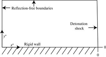
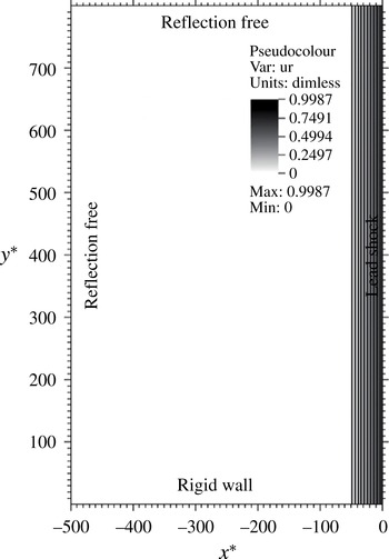
The spatial domain for the problem described in figure 7 and now expressed in the shock-attached coordinates given in (5.22) is the rectangular domain displayed in figure 8. Application of the reflection-free boundary conditions (continuation conditions) on the top and left boundaries is straightforward, as is the condition
 $({\mathcal{V}})_{y^{\ast }=0}=0$
along the rigid wall. Some further development is required to define the boundary conditions to be applied at the shock,
 $x^{\ast }=0$
.
The problem domain for the oblique detonation rigid-wall interaction problem displayed in figure 7. Here, the problem domain is displayed in shock-attached coordinates.

Using (3.3)–(3.4) along with the definition of
 $\boldsymbol{n}\boldsymbol{\cdot }\boldsymbol{U}_{lab}=P/(\unicode[STIX]{x1D70C}_{0}D_{CJ}\sqrt{f})$
at the shock, we can solve to get the leading-order result for the shock condition for
 $\boldsymbol{n}\boldsymbol{\cdot }\boldsymbol{U}_{lab}$
,
 $$\begin{eqnarray}\left(\frac{\boldsymbol{n}\boldsymbol{\cdot }\boldsymbol{U}_{lab}}{U_{CJ}}\right)_{+}=\unicode[STIX]{x1D716}+\sqrt{1+\unicode[STIX]{x1D716}^{2}},\end{eqnarray}$$
with the overdrive
 $f$
given by (3.4),
 $$\begin{eqnarray}f=\frac{D_{n}^{2}}{D_{CJ}^{2}}=1+\unicode[STIX]{x1D716}^{2}.\end{eqnarray}$$
The fact that
 $$\begin{eqnarray}\boldsymbol{n}\boldsymbol{\cdot }\boldsymbol{U}_{lab}=(\tilde{u} _{x}+D_{CJ}/\cos \unicode[STIX]{x1D719}_{e})\cos \unicode[STIX]{x1D719}+\tilde{u} _{y}\sin \unicode[STIX]{x1D719},\end{eqnarray}$$
which through first order can be written as
 $$\begin{eqnarray}\frac{\boldsymbol{n}\boldsymbol{\cdot }\boldsymbol{U}_{lab}}{U_{CJ}}=1+\unicode[STIX]{x1D6FF}\frac{\tilde{u} _{x}^{(1)}}{U_{CJ}}+O(\unicode[STIX]{x1D6FF}^{2}),\end{eqnarray}$$
leads to
 $$\begin{eqnarray}\unicode[STIX]{x1D716}=\unicode[STIX]{x1D6FF}\left(\frac{\tilde{u} _{x}^{(1)}}{U_{CJ}}\right)_{+}+O(\unicode[STIX]{x1D6FF}^{2}),\end{eqnarray}$$
where
 $(+)$
indicates the shock state. This then leads to the result
 $$\begin{eqnarray}\frac{D_{n}}{D_{CJ}}=1+\frac{1}{2}\unicode[STIX]{x1D6FF}^{2}\left(\frac{\tilde{u} _{x}^{(1)}}{U_{CJ}}\right)_{+}^{2}+O(\unicode[STIX]{x1D6FF}^{3}).\end{eqnarray}$$
Using (4.31) and the result that
 $\unicode[STIX]{x2202}\tilde{\unicode[STIX]{x1D713}}_{s}/\unicode[STIX]{x2202}\bar{t}=O(\unicode[STIX]{x1D6FF}^{2})$
and
 $\unicode[STIX]{x2202}\tilde{\unicode[STIX]{x1D713}}_{s}/\unicode[STIX]{x2202}\bar{y}=O(\unicode[STIX]{x1D6FF}^{3/2})$
, it then follows from (4.28) that
 $$\begin{eqnarray}\frac{1}{D_{CJ}}\frac{\unicode[STIX]{x2202}\tilde{\unicode[STIX]{x1D713}}_{s}^{(1)}}{\unicode[STIX]{x2202}\bar{t}}=\frac{1}{2}\left(\frac{\tilde{u} _{x}^{(1)}}{U_{CJ}}\right)_{+}^{2}+O(\unicode[STIX]{x1D6FF}).\end{eqnarray}$$
Further, from (4.26) it follows that
 $$\begin{eqnarray}\left(\frac{\tilde{u} _{y}^{(3/2)}}{U_{CJ}}\right)_{+}=-\left(\frac{\tan \unicode[STIX]{x1D719}_{e}}{\unicode[STIX]{x1D6FF}^{3/2}}\right)-\left(\frac{\unicode[STIX]{x2202}\tilde{\unicode[STIX]{x1D713}}_{s}^{(1)}}{\unicode[STIX]{x2202}\bar{y}}\right),\end{eqnarray}$$
which on differentiating (6.7) with respect to
 $\bar{y}$
and (6.8) with respect to
 $\bar{t}$
yields on eliminating
 $\unicode[STIX]{x2202}^{2}\tilde{\unicode[STIX]{x1D713}}_{s}^{(1)}/\unicode[STIX]{x2202}\bar{t}\unicode[STIX]{x2202}\bar{y}$
the constraint on the solution at the shock,
 $$\begin{eqnarray}-\frac{1}{D_{CJ}}\frac{\unicode[STIX]{x2202}\;}{\unicode[STIX]{x2202}\bar{t}}\left(\frac{\tilde{u} _{y}^{(3/2)}}{U_{CJ}}\right)_{+}=\frac{1}{2}\frac{\unicode[STIX]{x2202}\;}{\unicode[STIX]{x2202}\bar{y}}\left(\frac{\tilde{u} _{x}^{(1)}}{U_{CJ}}\right)_{+}^{2}.\end{eqnarray}$$
On expressing the shock condition in the scaled coordinates of (5.21)–(5.22), we obtain
 $$\begin{eqnarray}-\frac{\unicode[STIX]{x2202}{\mathcal{V}}_{+}}{\unicode[STIX]{x2202}\unicode[STIX]{x1D70F}}=\frac{\unicode[STIX]{x2202}{\mathcal{U}}_{+}^{2}}{\unicode[STIX]{x2202}y^{\ast }}.\end{eqnarray}$$
Application of (6.10) at
 $x^{\ast }=0$
along with the other boundary conditions discussed earlier in this section gives a full description of the boundary conditions we apply to this UTSD model, (5.23)–(5.24). It is worth noting that this UTSD model was derived previously in a different context describing the progress of a transverse rarefaction into a two-dimensional reaction zone (Bdzil & Stewart Reference Bdzil and Stewart1986).
A brief word is in order on how we set the initial conditions for this problem. In our asymptotic analysis,
 $\unicode[STIX]{x1D719}_{e}=O(\unicode[STIX]{x1D6FF}^{3/2})$
(see the discussion preceding (5.7)). We introduce the order parameter
 $\tan A$
as our measure of the shock angle of the incident wave, where
 $$\begin{eqnarray}\tan \unicode[STIX]{x1D719}_{e}=\unicode[STIX]{x1D6FF}^{3/2}\tan A.\end{eqnarray}$$
Then, the initial conditions are set as
 $$\begin{eqnarray}\displaystyle & \displaystyle {\mathcal{U}}(\unicode[STIX]{x1D70F}=0,\ldots )=0, & \displaystyle\end{eqnarray}$$
 $$\begin{eqnarray}\displaystyle & \displaystyle {\mathcal{V}}(\unicode[STIX]{x1D70F}=0,\ldots )=-\frac{\tan A}{\sqrt{\unicode[STIX]{x1D6FC}}}, & \displaystyle\end{eqnarray}$$
the latter following from (4.26) and where
 $\unicode[STIX]{x1D6FC}$
is given by (5.21). This completes the problem specification. Next, we examine some of the mathematical properties of (5.23)–(5.24).
7 Unsteady transonic small-disturbance model properties
The UTSD equations (5.23)–(5.24) have a rich history, having been studied by Murman & Cole (Reference Murman and Cole1971), Ballhaus & Lomax (Reference Ballhaus and Lomax1975), Brio & Hunter (Reference Brio and Hunter1992), Tabak & Rosales (Reference Tabak and Rosales1994), Gamba, Rosales & Tabak (Reference Gamba, Rosales and Tabak1999), Hunter & Brio (Reference Hunter and Brio2000), Hunter & Tesdall (Reference Hunter and Tesdall2012), and others. Typically, they are studied in the limit of weak nonlinear acoustic waves propagating into a quiescent state. Their shock boundary condition is different from the one we find here, where we consider small perturbations to a strong CJ detonation propagating into quiescent unreacted explosive. Additionally, here we are in a lead-shock-attached frame, and so we can avoid the solution errors associated with lead-shock capturing.
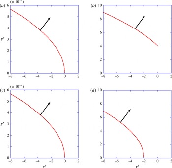
Four snapshots showing the wavefronts for a disturbance that emanates from
 $x^{\ast }=0$
,
 $y^{\ast }=0$
at
 $\unicode[STIX]{x1D70F}=0$
: (a,b) the case of subsonic flow,
 $B=1>0$
; (c,d) the case of supersonic flow,
 $B=-1<0$
.

To help to understand the wave properties of our model, we first linearize (5.23) about
 ${\mathcal{U}}=B$
, with
 $B$
a constant, and then introduce the velocity potential,
 $\unicode[STIX]{x1D6EF}$
, with
 ${\mathcal{U}}=\unicode[STIX]{x2202}\unicode[STIX]{x1D6EF}/\unicode[STIX]{x2202}x^{\ast }$
,
 ${\mathcal{V}}=\unicode[STIX]{x2202}\unicode[STIX]{x1D6EF}/\unicode[STIX]{x2202}y^{\ast }$
, to get
 $$\begin{eqnarray}\frac{\unicode[STIX]{x2202}^{2}\unicode[STIX]{x1D6EF}}{\unicode[STIX]{x2202}x^{\ast }\unicode[STIX]{x2202}\unicode[STIX]{x1D70F}}+B\frac{\unicode[STIX]{x2202}^{2}\unicode[STIX]{x1D6EF}}{\unicode[STIX]{x2202}{x^{\ast }}^{2}}+\frac{\unicode[STIX]{x2202}^{2}\unicode[STIX]{x1D6EF}}{\unicode[STIX]{x2202}{y^{\ast }}^{2}}=0.\end{eqnarray}$$
A straightforward characteristic analysis finds (7.1) to be hyperbolic and reducible to the canonical form of a two-dimensional wave equation
 $$\begin{eqnarray}\frac{\unicode[STIX]{x2202}^{2}\unicode[STIX]{x1D6EF}}{\unicode[STIX]{x2202}\unicode[STIX]{x1D709}_{1}^{2}}-\frac{\unicode[STIX]{x2202}^{2}\unicode[STIX]{x1D6EF}}{\unicode[STIX]{x2202}\unicode[STIX]{x1D709}_{2}^{2}}-\frac{\unicode[STIX]{x2202}^{2}\unicode[STIX]{x1D6EF}}{\unicode[STIX]{x2202}{y^{\ast }}^{2}}=0,\end{eqnarray}$$
where
 $$\begin{eqnarray}\unicode[STIX]{x1D709}_{1}=\unicode[STIX]{x1D70F}+\unicode[STIX]{x1D701},\quad \unicode[STIX]{x1D709}_{2}=-\unicode[STIX]{x1D70F}+\unicode[STIX]{x1D701},\quad \unicode[STIX]{x1D701}=B\unicode[STIX]{x1D70F}-x^{\ast },\end{eqnarray}$$
and where
 $\unicode[STIX]{x1D709}_{1}$
is the time-like variable. For this standard wave equation, the disturbance wavefront satisfies the characteristic equation (Eikonal)
 $$\begin{eqnarray}\left(\frac{\unicode[STIX]{x2202}\tilde{\unicode[STIX]{x1D6EF}}}{\unicode[STIX]{x2202}\unicode[STIX]{x1D709}_{1}}\right)^{2}-\left(\frac{\unicode[STIX]{x2202}\tilde{\unicode[STIX]{x1D6EF}}}{\unicode[STIX]{x2202}\unicode[STIX]{x1D709}_{2}}\right)^{2}-\left(\frac{\unicode[STIX]{x2202}\tilde{\unicode[STIX]{x1D6EF}}}{\unicode[STIX]{x2202}y^{\ast }}\right)^{2}=0,\end{eqnarray}$$
for which the general solution of (7.4) is of the form
 $$\begin{eqnarray}\tilde{\unicode[STIX]{x1D6EF}}\left(\sqrt{\unicode[STIX]{x1D709}_{2}^{2}+{y^{\ast }}^{2}}-C\mp \unicode[STIX]{x1D709}_{1}\right).\end{eqnarray}$$
Tracking the wavefront for a point disturbance emanating from
 $x^{\ast }=0$
,
 $y^{\ast }=0$
at
 $\unicode[STIX]{x1D70F}=0$
, we find that the evolving wavefront is given by
 $$\begin{eqnarray}{y^{\ast }}^{2}=4\unicode[STIX]{x1D70F}(B\unicode[STIX]{x1D70F}-x^{\ast }).\end{eqnarray}$$
Figure 9 features the wavefronts for the case of subsonic flow,
 $B=1>0$
(a,b), and the case of supersonic flow,
 $B=-1<0$
(c,d), with the early-time snapshots in (a,c) and the
 $\unicode[STIX]{x1D70F}=2$
snapshots in (b,d). The significant observation here is that the propagation speed to the left (backwards) is infinite. Since time in (7.1) is a characteristic direction, the domain of influence is unbounded. This property was described by Brio & Hunter (Reference Brio and Hunter1992). It is unique to the two-dimensional time-dependent problem (the characteristic speeds are finite for the related one-dimensional problem, the Burgers equation). This property results from the quasi-steady nature of the flow on the ordinary
 $t$
scale, equations (5.12)–(5.14), and from the slow time,
 $\unicode[STIX]{x1D70F}$
, being a characteristic direction of the linear problem. Essentially, any disturbance along the lower wall will formally be felt at
 $x^{\ast }\rightarrow -\infty$
for any
 $\unicode[STIX]{x1D70F}>0$
. The disturbance moves upwards at finite speed, having a limited zone of influence in the
 $y^{\ast }$
-direction. For the case of subsonic flow,
 $B=1>0$
, the upwards propagating wave intercepts the shock, while for supersonic flow,
 $B=-1<0$
, the upwards propagating wave falls further and further behind the shock (behind
 $x^{\ast }=0$
). These behaviours influence the properties that any numerical scheme we use must have to solve (5.23)–(5.24), (6.10) and (6.12)–(6.13).
Next, we describe how we solve the system of equations and boundary and initial conditions, (5.23)–(5.24), (6.10) and (6.12)–(6.13), with a joint implicit–explicit numerical solver.
8 Numerical solution strategy and algorithm
In the early 1970s, the steady-state form of (5.23)–(5.24) (albeit with a different shock condition) was of great interest in studying airfoils for high-speed subsonic and weakly transonic flight. The work of Murman & Cole (Reference Murman and Cole1971) was the first and most noteworthy. Now, in the case of steady flow, (5.23)–(5.24) become of mixed type, being hyperbolic in regions of supersonic flow and elliptic in regions of subsonic flow. To properly incorporate the mathematical properties of these equations, as we discussed in the previous section, Murman & Cole used an implicit central difference in the
 $y^{\ast }$
-direction to approximate
 $\unicode[STIX]{x2202}^{2}\unicode[STIX]{x1D6EF}/\unicode[STIX]{x2202}{y^{\ast }}^{2}$
. By also using an appropriate ‘upwind’ spatial difference in regions of supersonic flow and a central difference in subsonic regions to approximate
 $x^{\ast }$
-direction derivatives, they were able to devise a consistent and stable algorithm for describing such steady-state flows. Engquist & Osher (Reference Engquist and Osher1980) improved on this scheme by implementing a change in Murman & Cole’s
 $x^{\ast }$
-direction stencil switching to suppress the entropy violating expansion shocks permitted in Murman & Cole (Reference Murman and Cole1971). Ballhaus & Lomax (Reference Ballhaus and Lomax1975) devised a semi-implicit scheme for the time-dependent transonic equations, and demonstrated the feasibility of such methods for time-dependent problems. Further, for the two-dimensional time-dependent equations, Engquist & Osher (Reference Engquist and Osher1980) introduced a very stable scheme, where the
 $y^{\ast }$
-direction flow was solved for with an implicit method, using Crank–Nicolson type differencing. Brio & Hunter (Reference Brio and Hunter1992) employed a fully explicit Hamilton–Jacobi-equation-like scheme to solve the nearly acoustic weak Mach reflection for the equations for weakly transonic flow, equations similar to (5.23)–(5.24). Following on from the work of Murman & Cole (Reference Murman and Cole1971), Ballhaus & Lomax (Reference Ballhaus and Lomax1975) and Engquist & Osher (Reference Engquist and Osher1980), Hunter & Brio (Reference Hunter and Brio2000) later migrated to a more accurate mixed explicit–implicit scheme where, similarly to other previous work, they used a fully implicit time discretization for the diffraction term,
 $\unicode[STIX]{x2202}^{2}\unicode[STIX]{x1D6EF}/\unicode[STIX]{x2202}{y^{\ast }}^{2}$
. Recently, Faria, Kasimov & Rosales (Reference Faria, Kasimov and Rosales2015) used a scheme closely related to that of Hunter & Brio (Reference Hunter and Brio2000) to solve a two-dimensional UTSD model for the problem of detonation instability and cellular structure.
Here, we follow the early work (Murman & Cole Reference Murman and Cole1971; Ballhaus & Lomax Reference Ballhaus and Lomax1975; Engquist & Osher Reference Engquist and Osher1980, etc.) in using the velocity potential,
 $\unicode[STIX]{x1D6EF}$
, as the dependent variable. As in Hunter & Brio (Reference Hunter and Brio2000) and following Ballhaus & Lomax (Reference Ballhaus and Lomax1975), we use a fully implicit time discretization for the diffraction term
 $\unicode[STIX]{x2202}{\mathcal{V}}/\unicode[STIX]{x2202}y^{\ast }=\unicode[STIX]{x2202}^{2}\unicode[STIX]{x1D6EF}/\unicode[STIX]{x2202}{y^{\ast }}^{2}$
appearing in (5.23)–(5.24). In terms of the velocity potential
 $\unicode[STIX]{x1D6EF}$
, (5.23)–(5.24) can be written as
 $$\begin{eqnarray}\unicode[STIX]{x1D6EF}_{x^{\ast },\unicode[STIX]{x1D70F}}+1/2((\unicode[STIX]{x1D6EF}_{x^{\ast }})^{2})_{x^{\ast }}+\unicode[STIX]{x1D6EF}_{y^{\ast },y^{\ast }}=0,\end{eqnarray}$$
where henceforth subscripts denote partial derivatives with respect to the subscripted independent variables. With
 $\unicode[STIX]{x1D6EF}^{n}(x^{\ast },y^{\ast })$
representing the discretized solution at time-level
 $n$
,
 $$\begin{eqnarray}\unicode[STIX]{x1D6EF}^{n}(x^{\ast },y^{\ast })\approx \unicode[STIX]{x1D6EF}(x^{\ast },y^{\ast },n\unicode[STIX]{x0394}\unicode[STIX]{x1D70F}),\end{eqnarray}$$
in our numerical scheme, time discretization in (8.1) takes the form
 $$\begin{eqnarray}\left(\frac{\unicode[STIX]{x1D6EF}^{n+1}-\unicode[STIX]{x1D6EF}^{n}}{\unicode[STIX]{x0394}\unicode[STIX]{x1D70F}}+\frac{1}{2}\left(\unicode[STIX]{x1D6EF}_{x^{\ast }}^{n}\right)^{2}\right)_{x^{\ast }}+\unicode[STIX]{x1D6EF}_{y^{\ast },y^{\ast }}^{n+1}=0.\end{eqnarray}$$
We use a central-difference approximation for the spatial discretization of
 $\unicode[STIX]{x1D6EF}_{y^{\ast },y^{\ast }}^{n+1}$
,
 $$\begin{eqnarray}\unicode[STIX]{x1D6EF}_{y^{\ast },y^{\ast }}^{n+1}=(\unicode[STIX]{x1D6EF}_{i,j+1}^{n+1}-2\unicode[STIX]{x1D6EF}_{i,j}^{n+1}+\unicode[STIX]{x1D6EF}_{i,j-1}^{n+1})/(\unicode[STIX]{x0394}y^{\ast })^{2},\end{eqnarray}$$
and a forward-difference approximation for
 $\unicode[STIX]{x1D6EF}_{x^{\ast }}^{n}$
,
 $$\begin{eqnarray}\unicode[STIX]{x1D6EF}_{x^{\ast }}^{n}=(\unicode[STIX]{x1D6EF}_{i+1,j}^{n}-\unicode[STIX]{x1D6EF}_{i,j}^{n})/\unicode[STIX]{x0394}x^{\ast }.\end{eqnarray}$$
For the discretization of the
 $x^{\ast }$
-direction spatial operator,
 $((\unicode[STIX]{x1D6EF}_{x^{\ast }}^{n})^{2})_{x^{\ast }}/2$
, we note the similarity of this operator with (3.4) in Osher & Sethian (Reference Osher and Sethian1988),
 $$\begin{eqnarray}\unicode[STIX]{x1D6EF}_{x^{\ast },\unicode[STIX]{x1D70F}}+({\mathcal{H}}(\unicode[STIX]{x1D6EF}_{x^{\ast }}))_{x^{\ast }}=0,\end{eqnarray}$$
with
 ${\mathcal{H}}(\;)=(1/2)(\;)^{2}$
, and write
 $$\begin{eqnarray}\displaystyle \frac{1}{2}((\unicode[STIX]{x1D6EF}_{x^{\ast }}^{n})^{2})_{x^{\ast }} & = & \displaystyle \frac{1}{8(\unicode[STIX]{x0394}x^{\ast })^{3}} ((\text{max}((\unicode[STIX]{x1D6EF}_{i+1,j}^{n}-\unicode[STIX]{x1D6EF}_{i-1,j}^{n}),0))^{2}\nonumber\\ \displaystyle & & \displaystyle +\,(\text{min}((\unicode[STIX]{x1D6EF}_{i+2,j}^{n}-\unicode[STIX]{x1D6EF}_{i,j}^{n}),0))^{2}\nonumber\\ \displaystyle & & \displaystyle -\,(\text{max}((\unicode[STIX]{x1D6EF}_{i,j}^{n}-\unicode[STIX]{x1D6EF}_{i-2,j}^{n}),0))^{2}\nonumber\\ \displaystyle & & \displaystyle -\,(\text{min}((\unicode[STIX]{x1D6EF}_{i+1,j}^{n}-\unicode[STIX]{x1D6EF}_{i-1,j}^{n}),0))^{2} ).\end{eqnarray}$$
Combining the expressions in (8.3)–(8.7), we get
 $$\begin{eqnarray}\displaystyle \unicode[STIX]{x1D70E}\left(\unicode[STIX]{x1D6EF}_{i,j+1}^{n+1}-\left(2+\frac{1}{\unicode[STIX]{x1D70E}}\right)\unicode[STIX]{x1D6EF}_{i,j}^{n+1}+\unicode[STIX]{x1D6EF}_{i,j-1}^{n+1}\right)+\unicode[STIX]{x1D6EF}_{i+1,j}^{n+1}=\unicode[STIX]{x1D6EF}_{i+1,j}^{n}-\unicode[STIX]{x1D6EF}_{i,j}^{n}-\unicode[STIX]{x0394}\unicode[STIX]{x1D70F}\unicode[STIX]{x0394}x^{\ast }\frac{1}{2}((\unicode[STIX]{x1D6EF}_{x^{\ast }}^{n})^{2})_{x^{\ast }}, & & \displaystyle \nonumber\\ \displaystyle & & \displaystyle\end{eqnarray}$$
with
 $\unicode[STIX]{x1D70E}=\unicode[STIX]{x0394}\unicode[STIX]{x1D70F}\unicode[STIX]{x0394}x^{\ast }/\left(\unicode[STIX]{x0394}y^{\ast }\right)^{2}$
and where (8.8) represents our forward Euler in time, first order in space approximation to (8.1).
In our lead-shock-attached reference frame (see figure 8), where the lead shock is located in the rightmost
 $i$
-column (
 $i=im+1$
), the shock condition given by (6.10) replaces (8.8). Introducing the velocity potential,
 $\unicode[STIX]{x1D6EF}$
, into (6.10) and integrating the result with respect to
 $y^{\ast }$
then yields
 $$\begin{eqnarray}\unicode[STIX]{x1D6EF}_{i+1,j}^{n+1}=\unicode[STIX]{x1D6EF}_{i+1,j}^{n}+\unicode[STIX]{x0394}\unicode[STIX]{x1D70F}\cdot (1-((\unicode[STIX]{x1D6EF}_{i+1,j}^{n}-\unicode[STIX]{x1D6EF}_{i,j}^{n})/\unicode[STIX]{x0394}x^{\ast })^{2}),\end{eqnarray}$$
which is the discretized representation of the shock condition to be applied with
 $i=im$
. The remaining boundary conditions indicated in figure 8, which correspond to reflection-free and rigid-wall conditions, are applied via Engquist & Majda (Reference Engquist and Majda1981),
 $$\begin{eqnarray}\displaystyle & \unicode[STIX]{x1D6EF}_{0,j}^{n}=2\unicode[STIX]{x1D6EF}_{1,j}^{n}-\unicode[STIX]{x1D6EF}_{2,j}^{n}, & \displaystyle\end{eqnarray}$$
 $$\begin{eqnarray}\displaystyle & \unicode[STIX]{x1D6EF}_{i,jm+1}^{n}=2\unicode[STIX]{x1D6EF}_{i,jm}^{n}-\unicode[STIX]{x1D6EF}_{i,jm-1}^{n}, & \displaystyle\end{eqnarray}$$
 $$\begin{eqnarray}\displaystyle & \unicode[STIX]{x1D6EF}_{i,0}^{n}=\unicode[STIX]{x1D6EF}_{i,1}^{n}, & \displaystyle\end{eqnarray}$$
where the left, top and bottom boundary conditions are given by (8.10), (8.11) and (8.12) respectively. The domain displayed in figure 8 is covered by
 $1\leqslant i\leqslant im$
and
 $1\leqslant j\leqslant jm$
. The initial conditions (6.12)–(6.13) expressed in terms of
 $\unicode[STIX]{x1D6EF}$
and given on this mesh are
 $$\begin{eqnarray}\unicode[STIX]{x1D6EF}_{i,j}^{n}=-\left(\frac{\tan A}{\sqrt{\unicode[STIX]{x1D6FC}}}\right)\cdot j\unicode[STIX]{x0394}y^{\ast }.\end{eqnarray}$$
Restating the problem as a system of equations in matrix form, we write
 $$\begin{eqnarray}\unicode[STIX]{x1D63C}\boldsymbol{\cdot }\left(\begin{array}{@{}c@{}}\unicode[STIX]{x1D6EF}_{i,1}^{n+1}\\ \vdots \\ \unicode[STIX]{x1D6EF}_{i,j}^{n+1}\\ \vdots \\ \unicode[STIX]{x1D6EF}_{i,jm}^{n+1}\end{array}\right)=-\frac{1}{\unicode[STIX]{x1D70E}}\left(\begin{array}{@{}c@{}}\unicode[STIX]{x1D6EF}_{i+1,1}^{n+1}\\ \vdots \\ \unicode[STIX]{x1D6EF}_{i+1,j}^{n+1}\\ \vdots \\ \unicode[STIX]{x1D6EF}_{i+1,jm}^{n+1}\end{array}\right)+\frac{1}{\unicode[STIX]{x1D70E}}\left(\begin{array}{@{}c@{}}S_{i,1}^{n}\\ \vdots \\ S_{i,j}^{n}\\ \vdots \\ S_{i,jm}^{n}\end{array}\right),\end{eqnarray}$$
where
 $\unicode[STIX]{x1D63C}$
is the tridiagonal matrix
 $$\begin{eqnarray}\unicode[STIX]{x1D63C}=\left(\begin{array}{@{}ccccc@{}}-(2+1/\unicode[STIX]{x1D70E}) & 1 & 0 & \ldots \, & 0\\ 1 & -(2+1/\unicode[STIX]{x1D70E}) & 1 & 0 & \vdots \\ 0 & \ddots & \ddots & \ddots & 0\\ \vdots & 0 & 1 & -(2+1/\unicode[STIX]{x1D70E}) & 1\\ 0 & \ldots \, & 0 & 1 & -(2+1/\unicode[STIX]{x1D70E})\end{array}\right),\end{eqnarray}$$
being modified at the edges of the domain by the boundary conditions given by (8.10)–(8.12), and where the elements
 $S_{i,j}^{n}$
represent the source vector obtained from the right-hand side of (8.8).
Operationally, we first compute the source vector with the elements
 $\unicode[STIX]{x1D6EF}_{i+1,j}^{n+1}$
appearing on the right-hand side of (8.14) coming from the lead-shock condition (8.9). This then allows us to compute the elements
 $\unicode[STIX]{x1D6EF}_{i,j}^{n+1}$
by solving the matrix equation (8.14). Then, scanning in
 $i$
from right to left (for decreasing
 $i$
values) progressively, we compute
 $\unicode[STIX]{x1D6EF}_{i,j}^{n+1}$
over the entire domain,
 $1\leqslant i\leqslant im$
and
 $1\leqslant j\leqslant jm$
. Since the modified matrix
 $\unicode[STIX]{x1D63C}$
is mostly tridiagonal, except along top and bottom rows and the left column due to boundary condition application,
 $\unicode[STIX]{x1D63C}$
is easily invertible numerically, according to Press et al. (Reference Press, Teukolsky, Vetterling and Flannery1997). This then reduces finding the solution
 $\unicode[STIX]{x1D6EF}_{i,j}^{n+1}$
to a matrix–vector multiplication.
Next, we consider a simple verification problem to test our numerical algorithm and to test its accuracy. We consider a problem of a CJ detonation supported with the CJ state particle velocity, i.e.
 ${\mathcal{U}}=0$
. We take
 $\tan A=0$
, and so initially
 ${\mathcal{V}}=0$
as well. To these uniform initial data, we add a small circular region of radius
 $r_{c}$
, where
 ${\mathcal{U}}$
and
 ${\mathcal{V}}$
are non-zero, which serves to perturb the flow. We achieve this initial state with the initial velocity potential
 $$\begin{eqnarray}\displaystyle & \displaystyle \unicode[STIX]{x1D6EF}=\frac{A_{c}}{r_{c}}\sqrt{(x^{\ast }-x_{c}^{\ast })^{2}+(y^{\ast }-y_{c}^{\ast })^{2}}\quad \text{for }(x^{\ast }-x_{c}^{\ast })^{2}+(y^{\ast }-y_{c}^{\ast })^{2}\leqslant r_{c}^{2}, & \displaystyle\end{eqnarray}$$
 $$\begin{eqnarray}\displaystyle & \displaystyle \unicode[STIX]{x1D6EF}=A_{c}\quad \text{for }(x^{\ast }-x_{c}^{\ast })^{2}+(y^{\ast }-y_{c}^{\ast })^{2}>r_{c}^{2}, & \displaystyle\end{eqnarray}$$
where
 $A_{c}$
is the amplitude of the perturbation (taken to be very small) and
 $x_{c}^{\ast }$
,
 $y_{c}^{\ast }$
locates the centre of the circular perturbation. We solve this problem over the domain
 $-1000\leqslant x^{\ast }\leqslant 0$
and
 $0\leqslant y^{\ast }\leqslant 1000$
, with
 $(\unicode[STIX]{x2202}{\mathcal{V}}/\unicode[STIX]{x2202}y^{\ast })=0$
on the top and bottom boundaries,
 $(\unicode[STIX]{x2202}{\mathcal{U}}/\unicode[STIX]{x2202}x^{\ast })=0$
on the left boundary and the lead-shock condition (6.10) along the right boundary. The ABS model parameters are used.
We solve this problem with 8000 points in both the
 $x^{\ast }$
- and the
 $y^{\ast }$
-direction. The head and tail of the wave generated by this perturbation at
 $\unicode[STIX]{x1D70F}=60$
are located with the isosurface,
 $\unicode[STIX]{x1D6EF}=60.506$
. This closed contour is shaped like a thin boomerang, with a thickness of
 $2r_{c}$
. This solution of the weakly disturbed but nonlinear problem is compared with the expression for the wavehead coming from a point disturbance, given by (7.6), with
 $B=0$
,
 $$\begin{eqnarray}(y^{\ast }-y_{c}^{\ast })^{2}=4\unicode[STIX]{x1D70F}\cdot (x_{c}^{\ast }-x^{\ast }).\end{eqnarray}$$
This comparison is displayed in figure 10. The close agreement between simulation and theory, with (8.18) lying between the head and tail of the computed disturbance, serves to verify our numerical methodology.
A comparison of the computed
 $\unicode[STIX]{x1D6EF}=60.506$
contour at
 $\unicode[STIX]{x1D70F}=60$
with the analytical linear result for the disturbance wavehead (7.6). Here, we take
 $r_{c}=5$
,
 $A_{c}=0.5$
,
 $x_{c}^{\ast }=-50$
and
 $y_{c}^{\ast }=500$
. The linear analytical results are the two dashed curves nearer the tail of the wavehead. The curves are very close to one another.

In the next section, we explore the solutions for the CJ detonation Mach reflection problem.
9 Small-angle Mach reflection of a CJ detonation
The classical instantaneous reaction CJ detonation Mach reflection problem has been of interest for many years. In the area of condensed-phase explosives research, a problem of practical interest has to do with the pressure that an oblique detonation delivers to an adjacent inert material when Mach reflection occurs. To model this problem, Sternberg & Piacesi (Reference Sternberg and Piacesi1966) used a shock-polar approach similar to that described in the introduction. Although these authors make no clear statement about their assumptions for modelling the Mach reflection, they appear to have made the approximation of an essentially straight Mach stem, as later discussed by Law (Reference Law1970). In his work, Law used an iterative process to determine the angle that the Mach reflection triple-point path makes with the material interface. We use the model strategy for glancing incidence reflection of a CJ detonation developed here to solve for the included angle that the triple-point track makes with the surface of the incident detonation,
 $\unicode[STIX]{x1D714}_{M}$
(see figure 3). These results describe detonation Mach reflection when viewed on a scale of hundreds of reaction-zone lengths.
We set the parameters for our UTSD model to correspond to those of the ABS model,
 $$\begin{eqnarray}\unicode[STIX]{x1D70C}_{0}=2~\text{g}~\text{cm}^{-3},\quad \unicode[STIX]{x1D6FE}=3,\quad D_{CJ}=8~\text{mm}~\unicode[STIX]{x03BC}\text{s}^{-1},\end{eqnarray}$$
which yields the UTSD model parameter value
 $$\begin{eqnarray}\unicode[STIX]{x1D6FC}=\left(\frac{\unicode[STIX]{x1D6FE}+1}{\unicode[STIX]{x1D6FE}}\right)=\frac{4}{3},\end{eqnarray}$$
for which the unperturbed CJ detonation state is
 $$\begin{eqnarray}\displaystyle \left.\begin{array}{@{}c@{}}\unicode[STIX]{x1D70C}_{CJ}={\displaystyle \frac{\unicode[STIX]{x1D6FE}+1}{\unicode[STIX]{x1D6FE}}}\unicode[STIX]{x1D70C}_{0}={\displaystyle \frac{8}{3}}~\text{g}~\text{cm}^{-3},\quad P_{CJ}={\displaystyle \frac{\unicode[STIX]{x1D70C}_{0}D_{CJ}^{2}}{\unicode[STIX]{x1D6FE}+1}}=32~\text{GPa},\\ \tilde{u} _{CJ}=-{\displaystyle \frac{\unicode[STIX]{x1D6FE}}{\unicode[STIX]{x1D6FE}+1}}D_{CJ}=-6~\text{mm}~\unicode[STIX]{x03BC}\text{s}^{-1},\quad c_{CJ}=6~\text{mm}~\unicode[STIX]{x03BC}\text{s}^{-1}.\end{array}\right\} & & \displaystyle\end{eqnarray}$$
The angle of the incident detonation is set with the parameter
 $\tan A$
, which we span over the range
 $0.25\leqslant \tan A\leqslant 24.0$
. Our perturbation parameter,
 $\unicode[STIX]{x1D6FF}$
, is related to the degree of detonation overdrive
 $f=D_{n}^{2}/D_{CJ}^{2}=1+\unicode[STIX]{x1D716}^{2}$
with
 $\unicode[STIX]{x1D6FF}=O(\unicode[STIX]{x1D716})$
, which in turn is related to the angle of the incident detonation,
 $\unicode[STIX]{x1D719}_{e}$
, with
 $\unicode[STIX]{x1D719}_{e}=O(\unicode[STIX]{x1D6FF}^{3/2})$
, via
 $$\begin{eqnarray}\tan \unicode[STIX]{x1D719}_{e}=\unicode[STIX]{x1D6FF}^{3/2}\tan A.\end{eqnarray}$$
Although we display our results using the three independent variables
 $\unicode[STIX]{x1D70F}$
,
 $x^{\ast }$
and
 $y^{\ast }$
, the CJ detonation problem is scale-free and so is expressible in terms of the similarity variables
 $$\begin{eqnarray}\unicode[STIX]{x1D702}_{1}=\frac{x^{\ast }}{\unicode[STIX]{x1D70F}},\quad \unicode[STIX]{x1D702}_{2}=\frac{y^{\ast }}{\unicode[STIX]{x1D70F}}.\end{eqnarray}$$
In terms of these variables, (5.23)–(5.24) can be written as the second-order partial-differential equation (PDE)
 $$\begin{eqnarray}({\mathcal{U}}-\unicode[STIX]{x1D702}_{1}){\mathcal{U}}_{\unicode[STIX]{x1D702}_{1}\unicode[STIX]{x1D702}_{1}}-\unicode[STIX]{x1D702}_{2}{\mathcal{U}}_{\unicode[STIX]{x1D702}_{1}\unicode[STIX]{x1D702}_{2}}+({\mathcal{U}}_{\unicode[STIX]{x1D702}_{1}}-1){\mathcal{U}}_{\unicode[STIX]{x1D702}_{1}}=0.\end{eqnarray}$$
Equation (9.6) is hyperbolic when
 $$\begin{eqnarray}{\textstyle \frac{1}{4}}\unicode[STIX]{x1D702}_{2}^{2}+\unicode[STIX]{x1D702}_{1}-{\mathcal{U}}>0\end{eqnarray}$$
and is elliptic otherwise, with the sonic locus given by
 $$\begin{eqnarray}{\textstyle \frac{1}{4}}\unicode[STIX]{x1D702}_{2}^{2}+\unicode[STIX]{x1D702}_{1}-{\mathcal{U}}=0.\end{eqnarray}$$
The shock condition transforms to
 $$\begin{eqnarray}\unicode[STIX]{x1D702}_{2}\frac{\unicode[STIX]{x2202}{\mathcal{V}}_{+}}{\unicode[STIX]{x2202}\unicode[STIX]{x1D702}_{2}}=\frac{\unicode[STIX]{x2202}{\mathcal{U}}_{+}^{2}}{\unicode[STIX]{x2202}\unicode[STIX]{x1D702}_{2}},\end{eqnarray}$$
and thus the problem admits a self-similar solution. We will only use (9.8) to locate the sonic locus. Given the self-similar nature of this flow, the triple-point trajectory defined by our solution in
 $\unicode[STIX]{x1D70F}$
,
 $x^{\ast }$
,
 $y^{\ast }$
-space will be a straight line, given as
 $\unicode[STIX]{x1D702}_{2}=\text{const.}$
The
 ${\mathcal{U}}$
(a) and
 ${\mathcal{V}}$
(b) contours at
 $\unicode[STIX]{x1D70F}=200$
, with
 $\unicode[STIX]{x1D6FC}=4/3$
and
 $\tan A=1.0$
, for the initial boundary value problem given by (5.23)–(5.24), (6.10) and (6.12)–(6.13) and displayed in figures 7 and 8. A well-defined reflected shock forms and propagates upwards. The triple-point location is defined by the intersection of the reflected shock with the lead shock (
 $x^{\ast }=0$
). The Mach shock corresponds to the smoothly curved
 $x^{\ast }=0$
lead shock located below the triple point. (Note: the Mach shock is curved, as indicated by the intersection of the various contours with
 $x^{\ast }=0$
.) A jump in
 ${\mathcal{U}}$
and
 ${\mathcal{V}}$
(and also in pressure) is observed at the triple point. The sonic locus is coincident with the reflected shock. The flow below the sonic locus is subsonic. The contour spacing is
 $\unicode[STIX]{x0394}{\mathcal{U}}=\unicode[STIX]{x0394}{\mathcal{V}}=0.025$
, with
 ${\mathcal{U}}_{max}=0.785$
observed in the lower right-hand corner and
 ${\mathcal{V}}_{max}=-0.01$
along the
 $y^{\ast }=0$
axis.

Snapshots showing
 ${\mathcal{U}}$
and
 ${\mathcal{V}}$
at
 $\unicode[STIX]{x1D70F}=200$
for the initial boundary value problem for the case
 $\tan A=1.0$
, described in figures 7 and 8, are displayed in figure 11. The computational domain has
 $-500\leqslant x^{\ast }\leqslant 0$
and
 $0\leqslant y^{\ast }\leqslant 800$
, with the grid spacing set at
 $\unicode[STIX]{x0394}x^{\ast }=\unicode[STIX]{x0394}y^{\ast }=0.125$
. The time step is set as
 $\unicode[STIX]{x0394}\unicode[STIX]{x1D70F}=cfl\cdot \unicode[STIX]{x0394}x^{\ast }$
, with
 $cfl=0.1$
, although a constraint on
 $\unicode[STIX]{x0394}\unicode[STIX]{x1D70F}$
is not required by our implicit solver. Contours are shown with spacing
 $\unicode[STIX]{x0394}{\mathcal{U}}=\unicode[STIX]{x0394}{\mathcal{V}}=0.025$
. A clearly defined reflected shock develops and is seen to move upwards, separating the incident state (above) from the high-pressure Mach reflection state (below). A jump in
 ${\mathcal{U}}$
and
 ${\mathcal{V}}$
is observed at the triple point, with the Mach shock being broadly curved. The sonic locus is found to be coincident with the reflected shock.
A series of profiles along lines of constant
 $x^{\ast }$
, for
 $x^{\ast }=0,-100$
in steps of
 $\unicode[STIX]{x0394}x^{\ast }=-20$
, show
 ${\mathcal{U}}$
and
 ${\mathcal{V}}$
for the problem described in figure 11. The fan-like nature of
 ${\mathcal{U}}$
near the reflected shock is apparent. Unlike the
 ${\mathcal{U}}$
profiles, the
 ${\mathcal{V}}$
profiles experience a more modest change as one drops back from the lead shock.

A detailed examination of the flow along lines of constant
 $x^{\ast }$
, displayed in figure 12, shows the flow below the reflected shock to be smooth, which is consistent with the subsonic character of the flow in that region. The fan-like contours for
 ${\mathcal{U}}$
near the wavehead are a consequence of a decreasing
 ${\mathcal{U}}$
as one moves out along the reflected shock in this subsonic flow region. Near the wavehead,
 ${\mathcal{V}}$
is observed to be nearly constant as one moves out along the reflected shock.
Figure 13 shows the
 ${\mathcal{U}}$
and
 ${\mathcal{V}}$
profiles along the lead shock, displayed for different values of
 $\unicode[STIX]{x1D70F}$
. Five lead-shock profiles are displayed: the leftmost corresponds to
 $\unicode[STIX]{x1D70F}=25$
, with profiles for
 $\unicode[STIX]{x1D70F}=50$
, 100, 150 and 200 respectively as one moves to the right. For each profile, when moving from right to left along the
 $y^{\ast }$
-axis, one first encounters the reflected shock, and then smoothly increasing profiles in both
 ${\mathcal{U}}$
and
 ${\mathcal{V}}$
, ending at the state along the rigid horizontal surface at
 $y^{\ast }=0$
. The values of
 ${\mathcal{U}}$
and
 ${\mathcal{V}}$
at the intersection of the reflected shock and the Mach shock are nearly constant in time (which is expected), with
 ${\mathcal{U}}_{+}=0.55$
and
 ${\mathcal{V}}_{+}=-0.55$
.
Five snapshots, at
 $\unicode[STIX]{x1D70F}=25$
, 50, 100, 150 and 200, showing
 ${\mathcal{U}}$
and
 ${\mathcal{V}}$
along the lead shock, from the incident state at large
 $y^{\ast }$
to the highest-pressure Mach stem state at
 $y^{\ast }=0$
. The problem parameters are those described in figure 11. The Mach state at the triple point is
 ${\mathcal{U}}_{+}=0.55$
and
 ${\mathcal{V}}_{+}=-0.55$
.

With the pre-multiplying factor,
 $\unicode[STIX]{x1D702}_{2}$
, in (9.9) corresponding to the speed of the reflected shock in the direction of the incident shock, we can integrate (9.9) to get the condition for the speed of the triple point in the
 $y^{\ast }$
-direction,
 $$\begin{eqnarray}D_{T}=\frac{[{\mathcal{U}}_{+}^{2}]}{[{\mathcal{V}}_{+}]},\end{eqnarray}$$
where
 $[\;]$
represents the jump in the
 $y^{\ast }$
-direction across the reflected shock and the
 $(+)$
-subscript indicates that the variable is to be evaluated at the lead shock. With
 ${\mathcal{U}}=0.0$
and
 ${\mathcal{V}}=-0.866$
behind the incident detonation, it follows that
 $$\begin{eqnarray}D_{T}=0.96.\end{eqnarray}$$
The value of the triple-point speed in the
 $y^{\ast }$
-direction,
 $D_{T}$
, can also be computed directly from the shock shapes, where from (4.11) we have
 $$\begin{eqnarray}\unicode[STIX]{x1D713}_{s}(y,t)=(D_{CJ}/\cos \unicode[STIX]{x1D719}_{e})t+y\tan \unicode[STIX]{x1D719}_{e}+\tilde{\unicode[STIX]{x1D713}}_{s}(y,t),\end{eqnarray}$$
and where
 $(D_{CJ}/\cos \unicode[STIX]{x1D719}_{e})t$
describes the translation in laboratory space of the incident shock. Justifying all of the evolving shocks to
 $(D_{CJ}/\cos \unicode[STIX]{x1D719}_{e})t$
, the lead shock can simply be described by
 $\tilde{\unicode[STIX]{x1D713}}_{s}(y,t)$
. Then, when written in terms of our scaled variables, given by (5.22), we have
 $$\begin{eqnarray}\tilde{\unicode[STIX]{x1D713}}_{s}(y,t)=\unicode[STIX]{x1D6FF}\frac{2D_{CJ}}{\unicode[STIX]{x1D6FC}}\unicode[STIX]{x1D713}_{s}^{\ast }(y^{\ast },\unicode[STIX]{x1D70F}),\end{eqnarray}$$
with
 $$\begin{eqnarray}\frac{\unicode[STIX]{x2202}\unicode[STIX]{x1D713}_{s}^{\ast }}{\unicode[STIX]{x2202}\unicode[STIX]{x1D70F}}=-(1-({\mathcal{U}}_{+})^{2}),\end{eqnarray}$$
to get
 $$\begin{eqnarray}\unicode[STIX]{x1D713}_{s}(y,t)-(D_{CJ}/\cos \unicode[STIX]{x1D719}_{e})t=\unicode[STIX]{x1D6FF}\frac{2D_{CJ}}{\unicode[STIX]{x1D6FC}}\left(\frac{y^{\ast }\tan A}{\sqrt{\unicode[STIX]{x1D6FC}}}+\unicode[STIX]{x1D713}_{s}^{\ast }(y^{\ast },\unicode[STIX]{x1D70F})\right)\end{eqnarray}$$
as our scaled shock shape. Then, plotting
 $y^{\ast }\tan A/\sqrt{\unicode[STIX]{x1D6FC}}+\unicode[STIX]{x1D713}_{s}^{\ast }(y^{\ast },\unicode[STIX]{x1D70F})$
at the values
 $\unicode[STIX]{x1D70F}=0$
, 100 and 200, for the problem described in figure 11, we have the results displayed in figure 14.
The scaled shock shapes,
 $y^{\ast }\tan A/\sqrt{\unicode[STIX]{x1D6FC}}+\unicode[STIX]{x1D713}_{s}^{\ast }(y^{\ast },\unicode[STIX]{x1D70F})$
, versus
 $y^{\ast }$
plotted at
 $\unicode[STIX]{x1D70F}=0$
, 100 and 200 for the problem described in figure 11. A rough calculation shows that the upwards speed of the triple point is
 ${\approx}1.0$
. This compares with
 $D_{T}=0.96$
in our more precise calculation.

The speed of the triple point in the
 $y^{\ast }$
-direction, expressed in the units of our UTSD model and plotted as a function of the scaled incident shock-angle variable,
 $\tan A$
. Also shown is the function
 $S=(\tan A)^{1/3}$
.

Repeating the calculation for the model described in figure 11 for
 $\tan A=0.25$
, 0.5, 4.0, 8.0, 12.0 and 24.0, we find the results displayed in figure 15 for the
 $y^{\ast }$
-direction speed of the triple point as a function of
 $\tan A$
. The simple power-law fit
 $$\begin{eqnarray}S=(\tan A)^{1/3}\end{eqnarray}$$
replicates the data displayed in figure 15, where the triple-point speed in the
 $y^{\ast }$
-direction is
 $$\begin{eqnarray}\left(\frac{\text{d}y^{\ast }}{\text{d}\unicode[STIX]{x1D70F}}\right)_{TP}=S,\end{eqnarray}$$
which in unscaled coordinates is written as
 $$\begin{eqnarray}\left(\frac{\text{d}y}{\text{d}t}\right)_{TP}=\frac{D_{CJ}\sqrt{\unicode[STIX]{x1D6FF}}}{2\sqrt{\unicode[STIX]{x1D6FC}}}S.\end{eqnarray}$$
Now, combining this with the speed of the triple point in the
 $x$
-direction,
 $D_{CJ}/\cos \unicode[STIX]{x1D719}_{e}$
, we have as the velocity of the triple point
 $$\begin{eqnarray}\boldsymbol{v}_{TP}=\hat{i} \frac{D_{CJ}}{\cos \unicode[STIX]{x1D719}_{e}}+{\hat{j}}\frac{D_{CJ}\sqrt{\unicode[STIX]{x1D6FF}}}{2\sqrt{\unicode[STIX]{x1D6FC}}}S.\end{eqnarray}$$
In figure 16, we display this graphically, as in figure 3. Using (9.19), we can relate all the relevant angles of the triple-point flow to one another,
 $$\begin{eqnarray}\unicode[STIX]{x1D714}_{M}=\unicode[STIX]{x03C0}/2-\unicode[STIX]{x1D719}_{TP}-\unicode[STIX]{x1D719}_{e},\end{eqnarray}$$
where
 $\unicode[STIX]{x1D719}_{e}=O(\unicode[STIX]{x1D6FF}^{3/2})$
and
 $$\begin{eqnarray}\tan \unicode[STIX]{x1D719}_{TP}=\frac{\sqrt{\unicode[STIX]{x1D6FF}}\cos \unicode[STIX]{x1D719}_{e}}{2\sqrt{\unicode[STIX]{x1D6FC}}}S,\end{eqnarray}$$
with
 $\unicode[STIX]{x1D719}_{TP}=O(\unicode[STIX]{x1D6FF}^{1/2})$
. Since
 $$\begin{eqnarray}\sqrt{\unicode[STIX]{x1D6FF}}=\left(\frac{\tan \unicode[STIX]{x1D719}_{e}}{\tan A}\right)^{1/3},\end{eqnarray}$$
and
 $\unicode[STIX]{x1D719}_{TP}$
should depend on only
 $\unicode[STIX]{x1D6FC}$
and
 $\tan \unicode[STIX]{x1D719}_{e}$
, rewriting (9.21) we get
 $$\begin{eqnarray}S=\frac{2\sqrt{\unicode[STIX]{x1D6FC}}\tan \unicode[STIX]{x1D719}_{TP}}{(\tan \unicode[STIX]{x1D719}_{e})^{1/3}}(\tan A)^{1/3},\end{eqnarray}$$
and it follows from figure 15 that
 $$\begin{eqnarray}\tan \unicode[STIX]{x1D719}_{TP}=\frac{1}{2\sqrt{\unicode[STIX]{x1D6FC}}}(\tan \unicode[STIX]{x1D719}_{e})^{1/3},\end{eqnarray}$$
which for the ABS model parameters becomes
 $$\begin{eqnarray}\tan \unicode[STIX]{x1D719}_{TP}=0.433\cdots (\tan \unicode[STIX]{x1D719}_{e})^{1/3}.\end{eqnarray}$$
Equation (9.25) then summarizes the results of our numerical simulations, giving the track of the triple point as a function of
 $\tan \unicode[STIX]{x1D719}_{e}$
.
A diagram showing the lead shocks (incident and Mach) along with the track of the triple point. The angles
 $\unicode[STIX]{x1D719}_{e}$
,
 $\unicode[STIX]{x1D714}$
,
 $\unicode[STIX]{x1D719}_{TP}$
and
 $\unicode[STIX]{x1D714}_{M}$
are displayed.

Using (9.25), (9.20) and
 $\unicode[STIX]{x1D719}_{e}=O(\unicode[STIX]{x1D6FF}^{3/2})$
, we can compute the triple-point track. From our UTSD CJ detonation simulation results, we obtain the Mach stem pressure at the triple point using
 $$\begin{eqnarray}P_{M}=P_{CJ}(1+\unicode[STIX]{x1D6FF}{\mathcal{U}}_{M}),\end{eqnarray}$$
where the
 $M$
-subscript denotes the state at the Mach stem triple point. The results from the UTSD simulations for a number of cases are displayed in table 1, with
 $P_{CJ}=32~\text{GPa}$
.
The shock-polar diagram showing the reflected shock polar and Mach stem polar for the ABS model with
 $\unicode[STIX]{x1D714}=80^{\circ }$
(
 $\unicode[STIX]{x1D719}_{e}=10^{\circ }$
) and the value of
 $\unicode[STIX]{x1D714}_{M}=76.4^{\circ }$
, which is determined in the UTSD simulation.

A list of the results from two UTSD simulations for the ABS CJ detonation model, with
 $\tan A=1.0$
and
 $\tan A=8.0$
, and for three incident detonation angles,
 $\unicode[STIX]{x1D719}_{e}=5^{\circ }$
,
 $\unicode[STIX]{x1D719}_{e}=10^{\circ }$
and
 $\unicode[STIX]{x1D719}_{e}=15^{\circ }$
.

a See figure 13.
Using the listed values of
 $\unicode[STIX]{x1D714}_{M}$
for the three incident detonation angles given in table 1, we can perform the shock-polar calculations described in § 2, and compare the Mach stem pressures obtained with the polar calculations with the values listed in table 1. The shock-polar calculations yield
 $P_{M}=35.2~\text{GPa}$
(
 $\unicode[STIX]{x1D714}_{M}=79.1^{\circ }$
),
 $P_{M}=37.0~\text{GPa}$
(
 $\unicode[STIX]{x1D714}_{M}=76.4^{\circ }$
) and
 $P_{M}=38.2~\text{GPa}$
(
 $\unicode[STIX]{x1D714}_{M}=74.9^{\circ }$
) for the
 $\unicode[STIX]{x1D719}_{e}=5^{\circ }$
,
 $\unicode[STIX]{x1D719}_{e}=10^{\circ }$
and
 $\unicode[STIX]{x1D719}_{e}=15^{\circ }$
cases respectively. Figure 17 displays the shock-polar diagram for
 $\unicode[STIX]{x1D714}=80^{\circ }$
and
 $\unicode[STIX]{x1D714}_{M}=76.4^{\circ }$
, for which the Mach stem triple-point pressure is
 $P_{M}=37.0~\text{GPa}$
. This compares with the UTSD simulation Mach stem triple-point pressure of
 $P_{M}=37.5~\text{GPa}$
. The solutions described in this section represent the first detailed oblique detonation interaction simulations for a CJ detonation at glancing incidence. Among the findings are the following: (i) a classical triple-shock configuration is observed for glancing detonation incidence, so that the compressive energy generated by the detonation/wall interaction is carried by a sharp wavehead, (ii) the Mach stem is substantially curved and (iii) the track of the triple point follows a track given by (9.25), so that the track is very sensitive to the oblique shock angle,
 $\unicode[STIX]{x1D719}_{e}$
, for small values of
 $\unicode[STIX]{x1D719}_{e}$
.
The Hugoniot diagram for a one-dimensional quasi-steady detonation. Hugoniots are displayed for 0 % (chain-dashed), 80 % (dashed) and 100 % (solid) energy release. Three Rayleigh lines are displayed: (1) the CJ Rayleigh line for 80 % energy release (short-dashed), (2) the CJ Rayleigh line for 100 % energy release (solid) and (3) the overdriven Rayleigh line for the 100 % energy release Hugoniot with
 $f=1.2$
(long-dashed). In our discussion, we consider an SRHR model detonation, where the fraction of energy,
 $1-\unicode[STIX]{x1D6FF}^{2}$
, with
 $\unicode[STIX]{x1D6FF}^{2}\ll 1$
, is released instantaneously. The example shown considers the case
 $\unicode[STIX]{x1D6FF}^{2}=0.2$
, our condensed-phase EOS model with ABS parameters. The remaining energy fraction,
 $\unicode[STIX]{x1D6FF}^{2}$
, is released via a spatially resolved reaction. With no loss in generality, the resolved-energy release parameter,
 $\unicode[STIX]{x1D6FF}^{2}$
, that we use here is taken to be identical to the transverse flow/overdrive parameter introduced earlier.

In the next section, we briefly describe how resolving the detonation reaction zone diffuses the triple-shock configuration and produces a flow more akin to the smooth transition between the incident and Mach shocks observed for a von Neumann-type Mach reflection (Colella & Henderson Reference Colella and Henderson1990).
10 Resolved reaction-zone detonation Mach reflection: the SRHR model
Here, we consider that a small fraction of the energy release of our condensed-phase EOS explosive model, described in § 2, is spatially resolved. Using the equation of state given by (2.1), we repeat the mass, momentum and energy conservation arguments to obtain the one-dimensional quasi-steady Hugoniot diagram for a resolved-energy release detonation, where in place of (3.1) we have in the limit
 $M_{j}\rightarrow \infty$
 $$\begin{eqnarray}\left(1-\frac{\unicode[STIX]{x1D70C}_{0}^{2}}{\unicode[STIX]{x1D70C}^{2}}\right)\frac{D_{n}^{2}}{2}-\frac{\unicode[STIX]{x1D6FE}}{\unicode[STIX]{x1D6FE}+1}\frac{P}{\unicode[STIX]{x1D70C}_{0}}\frac{\unicode[STIX]{x1D70C}_{0}}{\unicode[STIX]{x1D70C}}+\frac{D_{CJ}^{2}\unicode[STIX]{x1D706}}{2(\unicode[STIX]{x1D6FE}^{2}-1)}=0.\end{eqnarray}$$
Eliminating
 $D_{n}$
through the Rayleigh line, equation (3.2), then yields
 $$\begin{eqnarray}\frac{P}{\unicode[STIX]{x1D70C}_{0}}\left(1-\left(\frac{\unicode[STIX]{x1D6FE}+1}{\unicode[STIX]{x1D6FE}-1}\right)\frac{\unicode[STIX]{x1D70C}_{0}}{\unicode[STIX]{x1D70C}}\right)+\frac{D_{CJ}^{2}\unicode[STIX]{x1D706}}{(\unicode[STIX]{x1D6FE}^{2}-1)}=0,\end{eqnarray}$$
where
 $D_{CJ}$
is the CJ detonation speed when all of the detonation energy is released and where
 $0\leqslant \unicode[STIX]{x1D706}\leqslant 1$
is the energy release fraction. We now introduce the instantaneous energy release fraction,
 $1-\unicode[STIX]{x1D6FF}^{2}$
, with
 $\unicode[STIX]{x1D6FF}^{2}\ll 1$
. With
 $\unicode[STIX]{x1D6FF}^{2}=0.2$
, setting
 $\unicode[STIX]{x1D706}$
in (10.2) to
 $\unicode[STIX]{x1D706}=0$
,
 $\unicode[STIX]{x1D706}=1-\unicode[STIX]{x1D6FF}^{2}=0.8$
or
 $\unicode[STIX]{x1D706}=1$
yields the 0 %, 80 % and 100 % energy release Hugoniots respectively. These Hugoniots are displayed in figure 18. When only a small fraction,
 $\unicode[STIX]{x1D6FF}^{2}=0.2$
, of the energy is released via resolved reactions, then the lead detonation shock resides on the short-dashed
 $P$
versus
 $\unicode[STIX]{x1D70C}_{0}/\unicode[STIX]{x1D70C}$
Hugoniot. If there were no further energy release, the Rayleigh line (short-dashed) tangent to the short-dashed Hugoniot would then have a CJ pressure and detonation speed that were a fraction
 $\unicode[STIX]{x1D6FF}^{2}$
below the full-release Hugoniot, which is displayed as the solid curve. As the energy fraction
 $\unicode[STIX]{x1D6FF}^{2}$
contributes to the flow, the pressure at the lead shock can rise by an
 $O(\unicode[STIX]{x1D6FF})$
amount along the 80 % Hugoniot. The reaction-zone structure and accompanying flow variables that are then observed for the one-dimensional quasi-steady solution to the SRHR model are those intersections of the various Hugoniots to the right of the short-dashed Hugoniot and those Rayleigh lines that are to the right of the short-dashed Rayleigh line. For an unsupported detonation, the lead-shock pressure can rise to the point on the 80 % Hugoniot that intersects the solid Rayleigh line. For an overdriven detonation, such as observed in Mach reflection, the lead-shock pressure can rise above this intersection point on the short-dashed Hugoniot, corresponding to the intersection of the rightmost (long-dashed) Rayleigh line with the short-dashed Hugoniot. The shock pressures one sees with the SRHR model lie along the short-dashed Hugoniot, and change by an
 $O(\unicode[STIX]{x1D6FF})$
amount as
 $D_{n}/D_{CJ}$
changes by an
 $O(\unicode[STIX]{x1D6FF}^{2})$
amount (both above and below
 $D_{CJ}$
).
In the limit
 $M_{j}=D_{CJ}/\sqrt{\unicode[STIX]{x1D6FE}P_{0}/\unicode[STIX]{x1D70C}_{0}}\rightarrow \infty$
, the one-dimensional quasi-steady solution for the pressure through the SRHR reaction zone is given by
 $$\begin{eqnarray}P=\frac{\unicode[STIX]{x1D70C}_{0}D_{CJ}^{2}f}{\unicode[STIX]{x1D6FE}+1}\left(1+\sqrt{1-\frac{\unicode[STIX]{x1D706}}{f}}\right),\end{eqnarray}$$
where
 $f=1+\unicode[STIX]{x1D716}^{2}$
, with
 $\unicode[STIX]{x1D716}^{2}\ll 1$
, is the transverse flow overdrive factor and where
 $$\begin{eqnarray}\unicode[STIX]{x1D706}=1-O(\unicode[STIX]{x1D6FF}^{2}),\quad \unicode[STIX]{x1D6FF}^{2}\ll 1,\end{eqnarray}$$
is the detonation energy release fraction. Making these substitutions for
 $f$
and
 $\unicode[STIX]{x1D706}$
in (10.1)–(10.2), we get an order estimate for how the pressure depends on the overdrive and energy release in the quasi-steady SRHR model,
 $$\begin{eqnarray}P=\frac{\unicode[STIX]{x1D70C}_{0}D_{CJ}^{2}}{\unicode[STIX]{x1D6FE}+1}\left(1+\sqrt{\unicode[STIX]{x1D6FF}^{2}+\unicode[STIX]{x1D716}^{2}}\right)+O(\unicode[STIX]{x1D6FF}^{2})+O(\unicode[STIX]{x1D716}^{2}).\end{eqnarray}$$
In the previous sections, where we considered Mach reflection of a CJ detonation, we introduced an order parameter
 $\unicode[STIX]{x1D6FF}=O(\unicode[STIX]{x1D716})$
(see near (4.32)) to measure how the detonation overdrive produced by the oblique interaction of the CJ detonation with a rigid wall modified the detonation flow. Here,
 $\unicode[STIX]{x1D6FF}^{2}$
measures the amount of detonation energy release that is spatially resolved. Here, to get the strongest interaction between the resolved heat-release fraction and the overdrive resulting from the oblique detonation interaction with the rigid wall, (10.5) motivates us to take
 $\unicode[STIX]{x1D6FF}=O(\unicode[STIX]{x1D716})$
, where, without loss of generality, we can take
 $\unicode[STIX]{x1D6FF}=\unicode[STIX]{x1D716}$
in our perturbation analysis. In this asymptotic limit, we find that the resolved energy enters together with the two-dimensional flow into our Burgers equation model (5.23)–(5.24), to yield
 $$\begin{eqnarray}\displaystyle & \displaystyle \left(\frac{\unicode[STIX]{x2202}{\mathcal{U}}}{\unicode[STIX]{x2202}\unicode[STIX]{x1D70F}}\right)_{x^{\ast },y^{\ast }}+{\mathcal{U}}\left(\frac{\unicode[STIX]{x2202}{\mathcal{U}}}{\unicode[STIX]{x2202}x^{\ast }}\right)_{y^{\ast },\unicode[STIX]{x1D70F}}+\left(\frac{\unicode[STIX]{x2202}{\mathcal{V}}}{\unicode[STIX]{x2202}y^{\ast }}\right)_{x^{\ast },\unicode[STIX]{x1D70F}}=\mathit{Rate}, & \displaystyle\end{eqnarray}$$
 $$\begin{eqnarray}\displaystyle & \displaystyle \left(\frac{\unicode[STIX]{x2202}{\mathcal{V}}}{\unicode[STIX]{x2202}x^{\ast }}\right)_{y^{\ast },\unicode[STIX]{x1D70F}}-\left(\frac{\unicode[STIX]{x2202}{\mathcal{U}}}{\unicode[STIX]{x2202}y^{\ast }}\right)_{x^{\ast },\unicode[STIX]{x1D70F}}=0, & \displaystyle\end{eqnarray}$$
with
 $$\begin{eqnarray}\mathit{Rate}=-\frac{1}{2}\left(\frac{\unicode[STIX]{x2202}\tilde{\unicode[STIX]{x1D706}}}{\unicode[STIX]{x2202}x^{\ast }}\right)_{y^{\ast },\unicode[STIX]{x1D70F}}=k(1-\tilde{\unicode[STIX]{x1D706}})^{\unicode[STIX]{x1D708}},\end{eqnarray}$$
where
 $\unicode[STIX]{x1D706}=1-\unicode[STIX]{x1D6FF}^{2}(1-\tilde{\unicode[STIX]{x1D706}})$
,
 $\unicode[STIX]{x1D706}$
is the mass fraction of reaction products,
 $k$
is the reaction-rate constant and now
 $\unicode[STIX]{x1D708}$
is the reaction-depletion order, where
 $0\leqslant \tilde{\unicode[STIX]{x1D706}}\leqslant 1$
. Given that the heat release enters at
 $O(\unicode[STIX]{x1D6FF}^{2})$
, it follows that weak reaction state sensitivity does not enter this analysis. The shock condition (6.10) remains unchanged, as do the boundary conditions (see figure 8).
The initial configuration of the
 ${\mathcal{U}}$
field for the SRHR detonation for
 $\tan A=1.0$
,
 $\unicode[STIX]{x1D708}=1/2$
and
 $k=0.02$
. The boundary conditions that are applied are indicated. The
 ${\mathcal{V}}$
field is initially
 ${\mathcal{V}}=-1/\sqrt{\unicode[STIX]{x1D6FC}}\tan A$
and the ABS model parameters are used. The contour spacing is
 $\unicode[STIX]{x0394}{\mathcal{U}}=0.1$
, with
 ${\mathcal{U}}_{max}=1.0$
and
 ${\mathcal{U}}_{min}=0.0$
.

The
 ${\mathcal{U}}$
(a) and
 ${\mathcal{V}}$
(b) fields at
 $\unicode[STIX]{x1D70F}=25$
for the SRHR model with
 $\tan A=1.0$
,
 $\unicode[STIX]{x1D708}=1/2$
,
 $k=0.02$
and the ABS model parameters. The compression wave is relatively well defined as the disturbance wavehead in the reaction zone. The reflected compression wave becomes relatively more diffuse behind the reaction zone. Even at early times, no reflected shock is evident. The contour spacing is
 $\unicode[STIX]{x0394}{\mathcal{U}}=0.1$
, with
 ${\mathcal{U}}_{max}=1.31$
and
 ${\mathcal{U}}_{min}=0.01$
, while
 $\unicode[STIX]{x0394}{\mathcal{V}}=0.05$
, with
 ${\mathcal{V}}_{max}=-0.01$
and
 ${\mathcal{V}}_{min}=-0.91$
.

The
 ${\mathcal{U}}$
(a) and
 ${\mathcal{V}}$
(b) fields at
 $\unicode[STIX]{x1D70F}=200$
for the SRHR model with
 $\tan A=1.0$
,
 $\unicode[STIX]{x1D708}=1/2$
,
 $k=0.02$
and the ABS model parameters. At this time, the lead shock is completely smooth, with no evidence of a reflected shock in the reaction zone. Very far back in the flow, a reflected wave is gaining definition over what is observed at
 $\unicode[STIX]{x1D70F}=25$
. However, no reflected shock is observed. The contour spacing is
 $\unicode[STIX]{x0394}{\mathcal{U}}=0.1$
, with
 ${\mathcal{U}}_{max}=1.31$
and
 ${\mathcal{U}}_{min}=0.01$
, while
 $\unicode[STIX]{x0394}{\mathcal{V}}=0.05$
, with
 ${\mathcal{V}}_{max}=-0.01$
and
 ${\mathcal{V}}_{min}=-0.91$
.

The
 ${\mathcal{U}}$
field along lines of constant
 $x^{\ast }$
, with
 $x^{\ast }=0$
,
 $-20$
,
 $-40$
,
 $-60$
,
 $-80$
and
 $-100$
at
 $\unicode[STIX]{x1D70F}=25$
(a) and
 $\unicode[STIX]{x1D70F}=200$
(b). The SRHR model parameters are
 $\tan A=1.0$
,
 $\unicode[STIX]{x1D708}=1/2$
,
 $k=0.02$
and the ABS model parameters. As one moves with increasing
 $y^{\ast }$
from the bottom boundary upwards, a reflected shock is present neither in the reaction zone nor in the flow following the reaction zone. The end of the reaction zone is at
 $x^{\ast }=-50$
. At
 $\unicode[STIX]{x1D70F}=200$
, the flow along the lead shock (upper curve in b) is fully smooth.

For initial conditions, we use the unsupported ZND detonation reaction zone plus the constant following flow state. Integration of (10.8) yields
 $$\begin{eqnarray}(1-\tilde{\unicode[STIX]{x1D706}})=(1+2(1-\unicode[STIX]{x1D708})kx^{\ast })^{1/1-\unicode[STIX]{x1D708}}.\end{eqnarray}$$
Using (10.3) and the perturbation expansions in § 5, we then have as initial conditions
 $$\begin{eqnarray}\displaystyle & \displaystyle {\mathcal{U}}(\unicode[STIX]{x1D70F}=0,\ldots )=\sqrt{1-\tilde{\unicode[STIX]{x1D706}}}, & \displaystyle\end{eqnarray}$$
 $$\begin{eqnarray}\displaystyle & \displaystyle {\mathcal{V}}(\unicode[STIX]{x1D70F}=0,\ldots )=-\frac{\tan A}{\sqrt{\unicode[STIX]{x1D6FC}}}. & \displaystyle\end{eqnarray}$$
We explore the solutions to this problem in the following section.
11 Mach reflection and resolved reaction zones: the SRHR model
The scaled independent and dependent variables are again given by (5.21)–(5.22). We retain the reaction-rate pre-multiplier in
 $\mathit{\{}$
, having
 $$\begin{eqnarray}\mathit{Rate}=k(1+2(1-\unicode[STIX]{x1D708})kx^{\ast })^{\unicode[STIX]{x1D708}/1-\unicode[STIX]{x1D708}}.\end{eqnarray}$$
For the examples we consider here, we take
 $\unicode[STIX]{x1D708}=1/2$
,
 $\unicode[STIX]{x1D708}=0.99$
and
 $\unicode[STIX]{x1D708}=1.51$
. We list the value of
 $k$
used in each of the simulation results we display. The half-reaction-zone length,
 $x\ast _{\unicode[STIX]{x1D706}=1/2}$
, is the same for all cases, being
 $x_{\unicode[STIX]{x1D706}=1/2}^{\ast }=14.645$
. Figure 19 displays the initial condition for
 ${\mathcal{U}}$
for the case
 $\unicode[STIX]{x1D708}=1/2$
and
 $k=0.02$
. The reaction-zone length is 50 units in the
 $x^{\ast }$
-direction. We first examine the case
 $\unicode[STIX]{x1D708}=1/2$
.
For our first example, we consider that
 $\tan A=1.0$
and the problem domain is
 $-500\leqslant x^{\ast }\leqslant 0$
and
 $0\leqslant y^{\ast }\leqslant 1000$
, with
 $\unicode[STIX]{x0394}x^{\ast }=\unicode[STIX]{x0394}y^{\ast }=0.125$
, which gives us 400 points in the reaction zone. Greyscale palette plots plus contours of the
 ${\mathcal{U}}$
and
 ${\mathcal{V}}$
solutions at
 $\unicode[STIX]{x1D70F}=25$
are displayed in figure 20.
What the plots in figure 20 show is a well-developed reflected wave (a compression wave and not a shock) propagating upwards. The interaction of the oblique detonation with the rigid wall at
 $y^{\ast }=0$
generates a significant increase in
 ${\mathcal{U}}$
(
 ${\mathcal{U}}$
can be thought of as pressure) in the reaction zone, with
 ${\mathcal{U}}=1.4$
as the highest lead-shock pressure compared with the incident detonation value of
 ${\mathcal{U}}=1.0$
. This is structurally a different result from that observed for the CJ detonation case, displayed in figure 11, where the reflected wave is a well-defined shock. Figure 21(a,b) displays
 ${\mathcal{U}}$
and
 ${\mathcal{V}}$
at
 $\unicode[STIX]{x1D70F}=200$
. It shows a diffuse reflected compression, and a totally smooth flow in the reaction zone from
 $y^{\ast }=0$
up into the regions that are totally undisturbed by the wall. Continuing, the plots in figure 22(a,b) display
 ${\mathcal{U}}$
versus
 $y^{\ast }$
at the fixed
 $x^{\ast }$
values of
 $x^{\ast }=0$
(lead shock),
 $-20$
,
 $-40$
,
 $-60$
,
 $-80$
and
 $-100$
. At both
 $\unicode[STIX]{x1D70F}=25$
and
 $\unicode[STIX]{x1D70F}=200$
, the
 ${\mathcal{U}}$
profiles are totally smooth, both in and behind the reaction zone. Thus, for the parameter values
 $\tan A=1.0$
,
 $\unicode[STIX]{x1D708}=1/2$
,
 $k=0.02$
, the Mach reflection at glancing incidence for the partially resolved reaction zone (the SRHR model) shows a totally smooth lead shock, with the reflected wave that forms behind the reaction zone being a weak very disperse compression wave. This is strikingly different from what is observed for the CJ detonation when
 $\tan A=1.0$
.
Next, we consider increasing the angle
 $\unicode[STIX]{x1D719}_{e}$
of the incident oblique detonation by taking
 $\tan A=8.0$
. We maintain the reaction-rate parameters at
 $\unicode[STIX]{x1D708}=1/2$
and
 $k=0.02$
, as in the previous example. Figures 23–25 display snapshots of the
 ${\mathcal{U}}$
and
 ${\mathcal{V}}$
fields at
 $\unicode[STIX]{x1D70F}=25$
and
 $\unicode[STIX]{x1D70F}=200$
. At
 $\unicode[STIX]{x1D70F}=25$
, we find a reasonably well-defined reflected shock in the reaction zone, but a diffuse reflected compression wave in the flow following the reaction zone (see figure 23). This is further confirmed by the
 ${\mathcal{U}}$
versus
 $y^{\ast }$
profiles at
 $x^{\ast }=0$
,
 $-20$
,
 $-40$
,
 $-60$
,
 $-80$
and
 $-100$
displayed at
 $\unicode[STIX]{x1D70F}=25$
in figure 26(a). As the flow develops further, at
 $\unicode[STIX]{x1D70F}=200$
we find that the reflected shock in the reaction zone has become a broad compression, while at the same time a well-defined reflected shock is observed in the flow following the reaction zone (see figures 24
a,b and 25). Particularly noteworthy is the expanded view of the reaction-zone
 ${\mathcal{U}}$
field in the vicinity of the wavehead separating the one-dimensional reaction-zone flow from the two-dimensional reaction-zone flow, which is displayed in figure 25. This figure clearly shows the smooth reflected wave in the reaction zone, steepening into a reflected shock as one moves back into the post-reaction-zone flow. This picture is further confirmed by the
 ${\mathcal{U}}$
versus
 $y^{\ast }$
profiles plotted at fixed
 $x^{\ast }$
values and displayed in figure 26(b). Comparing the snapshots of
 ${\mathcal{U}}$
at the wavehead in figures 25, 27 and 28, where we increase the reaction-depletion order,
 $\unicode[STIX]{x1D708}$
, while keeping the half-reaction length constant,
 $x_{\unicode[STIX]{x1D706}=0.5}^{\ast }=14.645$
, we find that as the heat-release rate is decreased (as
 $\unicode[STIX]{x1D708}$
is increased), we reach a point where the heat-release rate is less effective at turning the flow.
The
 ${\mathcal{U}}$
(a) and
 ${\mathcal{V}}$
(b) fields at
 $\unicode[STIX]{x1D70F}=25$
for the SRHR model with
 $\tan A=8.0$
,
 $\unicode[STIX]{x1D708}=1/2$
,
 $k=0.02$
and the ABS model parameters. A reflected shock is now relatively well defined as the disturbance wavehead in the reaction zone. The reflected shock becomes relatively more diffuse behind the reaction zone. The contour spacing is
 $\unicode[STIX]{x0394}{\mathcal{U}}=0.1$
, with
 ${\mathcal{U}}_{max}=3.41$
and
 ${\mathcal{U}}_{min}=0.01$
, while
 $\unicode[STIX]{x0394}{\mathcal{V}}=0.25$
, with
 ${\mathcal{V}}_{max}=-0.01$
and
 ${\mathcal{V}}_{min}=-7.01$
.

The
 ${\mathcal{U}}$
(a) and
 ${\mathcal{V}}$
(b) fields at
 $\unicode[STIX]{x1D70F}=200$
for the SRHR model with
 $\tan A=8.0$
,
 $\unicode[STIX]{x1D708}=1/2$
,
 $k=0.02$
and the ABS model parameters. At this time, the lead shock is completely smooth, with no evidence of a reflected shock in the reaction zone. Immediately behind the reaction zone, a reflected wave rapidly gains definition. The reaction-zone length is
 $x^{\ast }=50$
. The contour spacing is
 $\unicode[STIX]{x0394}{\mathcal{U}}=0.1$
, with
 ${\mathcal{U}}_{max}=3.41$
and
 ${\mathcal{U}}_{min}=0.01$
(with
 ${\mathcal{U}}_{max}$
in the lower right-hand corner), while
 $\unicode[STIX]{x0394}{\mathcal{V}}=0.25$
, with
 ${\mathcal{V}}_{max}=-0.01$
and
 ${\mathcal{V}}_{min}=-7.01$
(with
 ${\mathcal{V}}_{max}$
along
 $y^{\ast }=0$
).

The
 ${\mathcal{U}}$
field at
 $\unicode[STIX]{x1D70F}=200$
for the SRHR model with
 $\tan A=8.0$
,
 $\unicode[STIX]{x1D708}=1/2$
,
 $k=0.02$
and the ABS model parameters. A zoomed in view of
 ${\mathcal{U}}$
in the region of the wavehead is displayed for the results displayed for
 ${\mathcal{U}}$
in figure 24. The reflected shock in the flow behind the reaction zone becomes fully diffuse as one moves into the reaction zone. The full reaction-zone length is
 $x^{\ast }=50$
, while the half-reaction length is
 $x_{\unicode[STIX]{x1D706}=0.5}^{\ast }=14.645$
.

The
 ${\mathcal{U}}$
field along lines of constant
 $x^{\ast }$
, with
 $x^{\ast }=0$
,
 $-20$
,
 $-40$
,
 $-60$
,
 $-80$
and
 $-100$
at
 $\unicode[STIX]{x1D70F}=25$
(a) and
 $\unicode[STIX]{x1D70F}=200$
(b). The SRHR model parameters are
 $\tan A=8.0$
,
 $\unicode[STIX]{x1D708}=1/2$
,
 $k=0.02$
and the ABS model parameters. As one moves with increasing
 $y^{\ast }$
from the bottom boundary upwards, a reflected shock is observed to intersect the lead shock at
 $\unicode[STIX]{x1D70F}=25$
. The reflected shock becomes weaker as one drops back behind the reaction zone. At
 $\unicode[STIX]{x1D70F}=200$
, no reflected shock is observed in the reaction zone, but one is observed in the flow following the reaction zone. The end of the reaction zone is at
 $x^{\ast }=-50$
. At
 $\unicode[STIX]{x1D70F}=200$
, the flow along the lead shock (upper curve in b) is fully smooth.

A zoomed in view of the wavehead for the
 ${\mathcal{U}}$
field at
 $\unicode[STIX]{x1D70F}=200$
for the SRHR model with
 $\tan A=8.0$
,
 $\unicode[STIX]{x1D708}=0.99$
,
 $k=0.02358$
and the ABS model parameters. The reaction-rate constant,
 $k$
, is adjusted to make the half-reaction length
 $x_{\unicode[STIX]{x1D706}=0.5}^{\ast }=14.645$
, which is the same as for the case
 $\unicode[STIX]{x1D708}=1/2$
. The contour spacing is
 $\unicode[STIX]{x0394}{\mathcal{U}}=0.1$
. In the majority of the reaction zone, a broad reflected compression wave takes the place of the reflected shock observed for cases with smaller values of
 $\unicode[STIX]{x1D708}$
.

The
 ${\mathcal{U}}$
field at
 $\unicode[STIX]{x1D70F}=200$
for the SRHR model with
 $\tan A=8.0$
,
 $\unicode[STIX]{x1D708}=1.51$
,
 $k=0.02839$
and the ABS model parameters. The reaction-rate constant,
 $k$
, is adjusted to make the half-reaction length
 $x_{\unicode[STIX]{x1D706}=0.5}^{\ast }=14.645$
, which is the same as for the cases
 $\unicode[STIX]{x1D708}=1/2$
and
 $\unicode[STIX]{x1D708}=0.99$
. The contour spacing is
 $\unicode[STIX]{x0394}{\mathcal{U}}=0.1$
. The further broadening of the reaction zone decreases the local heat-release rate and its ability to turn the flow. Now, a very steep reflected compression wave is observed in the reaction zone, as compared with the case
 $\unicode[STIX]{x1D708}=0.99$
displayed in figure 27. As one moves further back in the reaction zone, the reflected compression wave steepens further.

Finally, we consider increasing the angle
 $\unicode[STIX]{x1D719}_{e}$
of the incident oblique detonation further, to
 $\tan A=24.0$
. Figure 29 displays a view focused near the wavehead for the
 ${\mathcal{U}}$
field at
 $\unicode[STIX]{x1D70F}=200$
. Now, we find a well-defined reflected shock extending from the lead shock fully back into the post-reaction-zone flow. The
 ${\mathcal{U}}$
versus
 $y^{\ast }$
profiles at fixed
 $x^{\ast }$
values displayed in figure 30 further confirm this picture, with both the reaction-zone and post-reaction-zone profiles showing a well-defined reflected shock.
A zoomed in view near the wavehead of the
 ${\mathcal{U}}$
field at
 $\unicode[STIX]{x1D70F}=200$
for the SRHR model with
 $\tan A=24.0$
,
 $\unicode[STIX]{x1D708}=1/2$
,
 $k=0.02$
and the ABS model parameters. For these model parameters and at this late time, the reflected shock is well defined in both the reaction zone and the flow following the reaction zone. The end of the reaction zone is at
 $x^{\ast }=-50$
. The contour spacing is
 $\unicode[STIX]{x0394}{\mathcal{U}}=0.2$
, with
 ${\mathcal{U}}_{max}=7.01$
and
 ${\mathcal{U}}_{min}=0.01$
(with
 ${\mathcal{U}}_{min}$
in the upper left-hand corner).

The
 ${\mathcal{U}}$
field along lines of constant
 $x^{\ast }$
, with
 $x^{\ast }=0$
,
 $-20$
,
 $-40$
,
 $-60$
,
 $-80$
and
 $-100$
at
 $\unicode[STIX]{x1D70F}=200$
. The SRHR model parameters are
 $\tan A=24.0$
,
 $\unicode[STIX]{x1D708}=1/2$
,
 $k=0.02$
and the ABS model parameters. As one moves with increasing
 $y^{\ast }$
from the bottom boundary upwards, a reflected shock is observed at all
 $x^{\ast }$
measuring stations.

The conclusion we draw from these observations of the solutions of the SRHR model is that a resolved reaction zone is effective at turning the flow for glancing attack angles of the incident detonation wave (this does not carry over to the large-wedge-angle case,
 $\tan A=24.0$
). For all of the examples we considered, the lead detonation shock is smooth, with there being no reflected shock intersecting the lead shock, in a three-shock configuration. For the CJ detonation cases, we observed a reflected shock intersecting the lead shock, in a three-shock configuration, for all of the examples we considered. Here, for all but the smallest incident shock angles (the
 $\tan A=1.0$
case), we find that as one moves into the post-reaction-zone flow, a reflected shock is seen to form, even in those cases (like
 $\tan A=8.0$
) where there is not a reflected shock in the reaction zone. Thus, as one drops back in the flow by a sufficiently large number of reaction-zone lengths, the flow resembles what we observed for the case of an instantaneous reaction CJ detonation.
What we observe is that the resolved reaction-zone heat release can itself work to turn the flow, without the benefit of having a reflected shock in the reaction zone. This behaviour is not observed for the CJ detonation model. Moreover, in the cases of resolved reaction zones that we consider, having no state sensitivity in the reaction rate, the smoothing of the reflected wave as it propagates upwards in the reaction zone seems to be associated with a wavehead, which itself moves at subacoustic speeds, with the majority of this energy moving upwards at a slower group velocity. For the case
 $\tan A=1.0$
and
 $k=0.02$
, the uppermost curve in figure 22(b) shows that the leading edge of the upwards propagating wave is located at
 $y^{\ast }\approx 400$
at
 $\unicode[STIX]{x1D70F}=200$
. There is only a barely perceptible shallow front propagating at the wavehead, with the bulk of this energy propagating at a slower speed. We note from (7.6) that the head of the upwards propagating acoustic wave along
 $x^{\ast }=0$
is located at
 $$\begin{eqnarray}y^{\ast }=2\unicode[STIX]{x1D70F}\sqrt{B},\end{eqnarray}$$
where
 $B=1$
for the unperturbed shock state of the one-dimensional incident wave. We observed the same effect in Bdzil & Stewart (Reference Bdzil and Stewart1986), where we were considering the progress of a lateral rarefaction into a two-dimensional detonation reaction zone.
One would expect to find a different result for the case where the detonation reaction rate was highly state sensitive, as in the case for gas detonation. However, in our modelling of condensed-phase heterogeneous explosive detonation, we are often led to weakly state sensitive reaction rates as being best able to describe the observed properties of detonation in these explosives. Thus, for the condensed-phase explosives that are the focus of our study, we do not expect the highly unstable situations that dominate in detonation of gas-phase explosives.
12 Conclusions
In this paper, we have explored how the finite length of a hydrodynamically stable detonation reaction zone influences Mach reflection for the case of glancing incidence of detonation off of a rigid wall. We performed this study using a rigorously derived asymptotic model of detonation, valid for the case where only a small fraction,
 $\unicode[STIX]{x1D6FF}^{2}\ll 1$
, of the total detonation energy is released via a resolved reaction, the SRHR model. In the dual limits of SRHR (
 $\unicode[STIX]{x1D6FF}^{2}\ll 1$
) and glancing incidence,
 $\tan \unicode[STIX]{x1D719}_{e}\ll 1$
, we derived
 $$\begin{eqnarray}\displaystyle \left.\begin{array}{@{}c@{}}\left(\displaystyle \frac{\unicode[STIX]{x2202}{\mathcal{U}}}{\unicode[STIX]{x2202}\unicode[STIX]{x1D70F}}\right)_{x^{\ast },y^{\ast }}+{\mathcal{U}}\left(\displaystyle \frac{\unicode[STIX]{x2202}{\mathcal{U}}}{\unicode[STIX]{x2202}x^{\ast }}\right)_{y^{\ast },\unicode[STIX]{x1D70F}}+\left(\displaystyle \frac{\unicode[STIX]{x2202}{\mathcal{V}}}{\unicode[STIX]{x2202}y^{\ast }}\right)_{x^{\ast },\unicode[STIX]{x1D70F}}=\mathit{Rate},\\ \left(\displaystyle \frac{\unicode[STIX]{x2202}{\mathcal{V}}}{\unicode[STIX]{x2202}x^{\ast }}\right)_{y^{\ast },\unicode[STIX]{x1D70F}}-\left(\displaystyle \frac{\unicode[STIX]{x2202}{\mathcal{U}}}{\unicode[STIX]{x2202}y^{\ast }}\right)_{x^{\ast },\unicode[STIX]{x1D70F}}=0,\end{array}\right\} & & \displaystyle\end{eqnarray}$$
the two-dimensional reactive Burgers equation UTSD model, here subject to the shock condition
 $$\begin{eqnarray}\displaystyle -\frac{\unicode[STIX]{x2202}{\mathcal{V}}_{+}}{\unicode[STIX]{x2202}\unicode[STIX]{x1D70F}}=\frac{\unicode[STIX]{x2202}{\mathcal{U}}_{+}^{2}}{\unicode[STIX]{x2202}y^{\ast }}. & & \displaystyle\end{eqnarray}$$
We first considered the generic CJ detonation Mach reflection problem for the case of glancing incidence, which can be studied by taking
 $\mathit{Rate}=0$
in the above equations. For this case, we found a classical three-shock Mach reflection. We determined the angle of the triple-point track, which for our ABS model is given by
 $$\begin{eqnarray}\displaystyle \tan \unicode[STIX]{x1D719}_{TP}=\frac{1}{2\sqrt{\unicode[STIX]{x1D6FC}}}(\tan \unicode[STIX]{x1D719}_{e})^{1/3}, & & \displaystyle\end{eqnarray}$$
where
 $\unicode[STIX]{x1D719}_{TP}$
is the triple-point angle and
 $\unicode[STIX]{x1D719}_{e}$
is the angle of the incident oblique CJ detonation (see figure 16 for the symbol definitions). We find that the Mach stem is quite curved for the case of CJ detonation Mach reflection. Using our derived
 $\unicode[STIX]{x1D719}_{TP}$
values in the shock-polar theory given in § 2 to compute the Mach stem pressure, we found those values to be in relatively good agreement with our simulated results of the UTSD theory pressures, measured at the triple point.
For the case of the SRHR model with the rate
 $$\begin{eqnarray}\displaystyle \mathit{Rate}=k(1+2(1-\unicode[STIX]{x1D708})kx^{\ast })^{\unicode[STIX]{x1D708}/(1-\unicode[STIX]{x1D708})} & & \displaystyle\end{eqnarray}$$
and
 $\unicode[STIX]{x1D708}=1/2$
, we found a Mach reflection looking more akin to von Neumann reflection. For the case where
 $\tan A$
is small, say
 $\tan A=1.0$
and
 $k=0.02$
, the lead detonation is completely smooth through the region of Mach reflection, with a reflected shock neither in the reaction zone nor in the flow following the reaction zone. As
 $\tan A$
was increased to
 $\tan A=8.0$
, we continued to see a smooth lead shock at long times and no reflected shock in the reaction zone. However, as we dropped back into the post-reaction-zone flow, a prominent reflected shock was seen to emerge. Further, going on to
 $\tan A=24.0$
, we then saw a reflected shock both in the reaction zone and continuing back into the post-reaction-zone flow. For this case, the lead shock showed a kink at the point where the reflected shock intersected it.
Thus, for smaller angles of incidence of the undisturbed lead detonation shock, as measured by
 $\tan A$
, all reflected waves are compressions and not shocks. As
 $\tan A$
was increased somewhat, we continued to not see a reflected shock in the reaction zone, but saw one develop in the post-reaction-zone flow. On further increasing
 $\tan A$
, we then saw reflected shocks both in the reaction zone and in the post-reaction-zone flow.
In the absence of instability in the detonation reaction zone, we found that the reaction-zone heat-release flow dynamics can itself turn the flow without a reflected shock being required for that purpose. Further, we solved the problem of Mach reflection for a CJ instantaneous reaction detonation. There, we found classical three-shock Mach reflection. We also found that the Mach stem was decidedly curved, and derived an expression for the angle of the triple-point track.
We only remark on here, but leave for a future paper, the results for the fully spatially resolved reaction-zone ABS model. Our high-resolution shock-capturing simulations for the Euler description of the fully resolved reaction zone using a high-resolution algorithm return essentially the same results as seen here when a two-step model approximating our SRHR model is used. Moreover, the results for the fully resolved one-step reaction model are similar in most respects to the results we have presented here for the SRHR model.
Acknowledgements
We thank T. Aslam for providing us with a two-dimensional Euler solver and J. Quirk for some simulation results, both used in our early preliminary investigations. This work was presented in part at the 25th ICDERS, 2–7 August 2015, Leeds, UK. This work is dedicated to Bill Davis in celebration of his 90th Birthday.