Nomenclature
-
 ${\phi _n}$
-
topological potential design variable at the n-th FE node
-
$r$
-
position vector in the design domain
-
$\Phi (\boldsymbol{r})$
-
continuous topological potential field interpolated from nodal variables
-
$\Psi (\boldsymbol{r},\lambda )$
-
relative topological potential field with global threshold-shift parameter
-
${\boldsymbol{u}_0}^{kl}$
-
affine initial displacement vector for the kl-th unit macroscopic strain case
-
$\lambda $
-
global threshold-shift parameter
-
${\rm{\Gamma }}$
-
material void topological boundary isosurface
-
$\boldsymbol{x}$
-
macroscopic coordinate
-
$\boldsymbol{y}$
-
microscopic coordinate
-
${v_e}$
-
effective volume fraction of the element
-
$d{c_e}$
-
element sensitivity of the positive stiffness objective with respect to
${v_e}$
-
${{\rm{\Omega }}_e}$
-
domain of the e-th finite element
-
${\xi _{m,e}}$
-
local coordinate vector of the m-th subgrid sampling point in element e
-
$\textrm{H}$
-
Heaviside projection operator
-
${\rm{\Theta (}}\boldsymbol{r}{\rm{)}}$
-
material-phase indicator function
-
$E_{ijkl}^{\text{H}}$
-
macroscopic effective elasticity tensor
-
$\boldsymbol{\bar{\varepsilon}}_{kl}$
-
kl-th unit macroscopic average strain
-
${\boldsymbol{\tilde {\chi}}}^{kl}$
-
periodic displacement correction field for the kl-th unit strain case
-
${\boldsymbol{F}^{kl}}$
-
induced equivalent nodal force vector for the kl-th unit strain case
-
${\boldsymbol{u}^\eta }$
-
multiscale displacement solution
-
$\boldsymbol{J}$
-
optimisation objective function
-
${w_{ab}}$
-
weighting coefficient of the performance component
-
${S_n}$
-
set of periodically adjacent elements sharing node n
-
$S$
-
set of performance metrics included in the objective function
-
$\boldsymbol{K}$
-
global stiffness matrix
-
${\boldsymbol{F}^{(k)}}$
-
equivalent nodal force vector for the k-th unit strain case
-
${\boldsymbol{U}^{(k)}}$
-
global displacement response of the unit cell under load case k
-
${\mathbf{R}_n}$
-
element-to-node sensitivity-mapping operator associated with node n


1.0 Introduction
Structural topology optimisation has become an important approach for material layout optimisation in advanced materials. It aims to achieve desired mechanical properties by tailoring the spatial distribution of materials within a prescribed design domain and under given constraints. Since Bendsøe [Reference Bendsøe and Kikuchi1] introduced the fundamental concept, Sigmund et al. [Reference Sigmund2] have opened a new route for microstructural configuration optimisation through inverse homogenisation design. On this basis, a variety of high-performance numerical algorithms have been developed in this field, including the Solid Isotropic Material with Penalisation (SIMP) method [Reference Sigmund3], the level set method (LSF) [Reference Challis, Roberts and Wilkins4], evolutionary structural optimisation (ESO) [Reference Huang, Radman and Xie5], the moving morphable components (MMC) method [Reference Zhang, Yuan, Zhang and Guo6] and isogeometric analysis (IGA) [Reference Gao, Wang, Luo and Gao7]. These classical algorithms not only exhibit excellent stability in macroscale structural design, but also provide a solid theoretical foundation for the design of microstructured materials. Studies have shown that, although microstructures are usually constructed from conventional base materials, scientifically designed topologies can still lead to excellent effective mechanical properties [Reference Cherkaev and Kohn8, Reference Torquato9]. In this field, microstructured materials are defined as periodic arrays composed of repeating unit cells, which can exhibit specific stiffness and specific strength at the macroscopic scale far exceeding those of the base materials [Reference Gibson and Ashby10, Reference Ashby, Evans, Fleck, Gibson, Hutchinson and Wadley11].
With the increasing maturity of design theories, extensive achievements have been made in the design of extremal properties, such as maximum bulk modulus [Reference Sigmund12], maximum shear modulus [Reference Huang, Radman and Xie5] and negative Poisson’s ratio [Reference Sigmund and Maute13]. In the field of microstructural design, functionally graded material design [Reference Paulino, Silva and Le14] represents another class of approaches closely related to periodic microstructures, while a further closely associated research direction is concurrent material-structure integrated design [Reference Rodrigues, Guedes and Bendsøe15]. To meet stability requirements in complex environments, Neves et al. [Reference Neves, Sigmund and Bendsøe16] investigated the configuration optimisation of porous materials against local instability using a two-scale asymptotic technique. Tajs et al. [Reference Tajs-Zielińska17] studied the topology optimisation of periodic structures subjected to self-weight loading using a heuristic method. In studies on lattice structures, Mistry et al. [Reference Mistry, Weeger, Morankar, Shinde, Liu, Chawla, Chen, Penick and Bhate18] developed highly compliant interwoven lattices inspired by biological structures. Abdullahi et al. [Reference Abdullahi, Zhuo, Fu and Gao19] established a high-quality unit-cell library, enabling the coordinated optimisation of microscopic cell selection and component dimensions. Chen et al. [Reference Chen, Baldwin, Narra and McComb20] proposed a generative lattice modeling method, providing an innovative technical route for multi-lattice topology optimisation.
Among various topology optimisation algorithms, the level set method has attracted considerable attention owing to the implicit nature of its geometric representation. Inspired by the pioneering work of Osher [Reference Osher and Sethian21] in interface tracking, Wang et al. [Reference Wang, Wang and Guo22] and Allaire et al. [Reference Allaire, Jouve and Toader23] successfully introduced the level set framework into topology optimisation, establishing an evolutionary paradigm that maintains clear boundaries and naturally accommodates topological changes. However, conventional level set methods usually require continuous evolution and numerical updating of the implicit boundary function. When applied to large-scale three-dimensional homogenisation problems, they often involve substantial computational costs associated with stability control, time marching and reinitialisation. To improve computational efficiency and enhance the generality of the algorithm, parameterised level set methods (PLSMs) have been further developed [Reference Wang and Wang24–Reference Luo, Tong and Kang26]. As stated by Van Dijk et al. [Reference Van Dijk, Maute, Langelaar and Van Keulen27] in their review, PLSMs transform the boundary evolution problem into a finite-parameter algebraic optimisation process through interpolation with spatial basis functions, thereby significantly improving numerical robustness and application flexibility. With the maturation of the underlying theory, topology optimisation has been increasingly applied to various engineering fields. Giorleo et al. [Reference Giorleo and Deniz28] achieved a substantial weight reduction of approximately 50% for an additively manufactured polymer bending tool while maintaining its structural function. Fu et al. [Reference Fu, Dong and Wang29] developed a collaborative nonlocal topology optimisation method to construct efficient graded acoustic metamaterials.
An evaluation of the aforementioned studies indicates that microstructural topology optimisation has made significant progress, yet there remains room for further improvement in specific scenarios. First, a key issue lies in balancing the accuracy of complex three-dimensional interface capture with computational cost. In large-scale three-dimensional homogenisation analyses, how to accurately represent interface details at the sub-element scale while maintaining a low number of finite element degrees of freedom remains an issue worthy of further investigation. Second, discrete error control in the physical mapping process also requires attention. Although conventional density-based methods are computationally efficient, their diffuse boundaries may lead to performance deviations during precision manufacturing and finite element validation. Third, performance adaptability under multiaxial loading environments remains challenging. Li [Reference Li, Li and Wang30], Ji [Reference Ji, Bai, Jiang, Liu, Yan and Han31], Daynes [Reference Daynes and Feih32], Wei [Reference Wei, Ye, Wang, Li, Tian and Sui33] and other researchers have made important contributions to concurrent optimisation and functionally graded lattices. However, for the design of sandwich-structure core materials, achieving deep coordination between supporting stiffness along the primary load-bearing direction and multidirectional shear resistance in space under extremely lightweight constraints remains a challenging balance in current evolutionary frameworks.
To address the aforementioned issues, this study employs an energy-based homogenisation method [Reference Xia and Breitkopf34] for effective property calculation and, on this basis, proposes a Threshold-Shift Boundary Evolution (TSBE) method. Specifically, element-wise sensitivity information is mapped onto the nodal space to construct a continuous topological potential field. A global threshold-shift parameter is then used to drive the boundary evolution between the material domain and the void domain, thereby achieving effective decoupling between smooth boundary representation and the finite element analysis mesh. Unlike the update logic of the conventional optimality criteria (OC) method [Reference Zhou and Rozvany35] or the Method of Moving Asymptotes (MMA) [Reference Svanberg36], the proposed framework reformulates material layout adjustment under a volume fraction constraint as a threshold optimisation problem in the scalar threshold space, which helps improve the computational efficiency and numerical stability of boundary updating. In addition, a subgrid integration technique is introduced to enhance the representation accuracy of smooth interfaces and material distributions on low-density analysis meshes. The stability of the proposed algorithm is first verified through extremal-performance unit-cell designs in two- and three-dimensional settings. Furthermore, to meet the lightweight design requirements of sandwich-structure core materials, topology optimization and numerical validation of functional cores are performed while considering both primary-direction supporting stiffness and multidirectional shear resistance. The main design route is shown in Fig. 1.
Schematic illustration of functional material design: (a) schematic of solid, void and boundary elements in the design domain; (b) boundary-evolution topology optimisation framework based on the nodal topological potential field and threshold-shift parameter; (c) HS-referenced performance ratios for the optimisation examples; (d) core performance indices for sandwich structures.

2.0 Theory of the threshold-shift boundary evolution method
2.1 Nodal parametric representation and threshold-based boundary description
This section establishes the threshold-sshift boundary evolution (TSBE) method. In this framework, a nodal topological potential field is employed as a continuous representation of material distribution, and a global threshold-shift parameter is used to regulate the position of the interface between the material domain and the void domain, thereby enabling the algebraic updating of topological boundaries. Unlike material distribution descriptions directly based on element densities, the TSBE method represents structural boundaries through potential-field interpolation in the nodal space and combines this representation with a threshold optimisation process in the scalar threshold space, thereby improving the computational efficiency and numerical stability of boundary evolution. This framework is designed to balance continuous boundary representation, interface characterisation accuracy on low-density meshes and the computational efficiency of scalar threshold calibration, providing a methodological basis for subsequent microstructural performance design. Within the design domain
 ${\rm{\Omega }} \subset {\mathbb{R}^d}(d = 2,3)$
, the set of nodal topological design variables
 $\phi = \left\{ {{\phi _1},{\phi _2}, \cdots {\phi _{{N_{node}}}}} \right\}$
is defined. Using the element shape functions
 ${N_i}(\boldsymbol{r})$
, a spatially continuous topological potential field
 $\Phi (\boldsymbol{r})$
is constructed within
 ${{\rm{\Omega }}_e}$
as follows:
 \begin{align} \Phi (\boldsymbol{r})=\sum\limits_{i = 1}^n {{N_i}(\boldsymbol{r})} {\phi _i} , \quad \boldsymbol{r} \in {\Omega _e} \end{align}
where
 $d$
denotes the dimension of the physical space,
 $i$
is the local node index,
 $\boldsymbol{r}$
is the continuous coordinate vector in the design domain,
 $n$
is the number of local nodes in the element,
 $\Phi (\boldsymbol{r})$
represents the spatially continuous topological potential distribution field generated by interpolation of the nodal variables and
 ${\phi _i}$
denotes the scalar topological-potential design variable defined at the finite element nodes. This nodal-field parameterisation process achieves effective decoupling between the geometric representation and the underlying finite element mesh, thereby overcoming the dependence of conventional density-based methods on mesh elements.
During the physical mapping process, a subgrid integration technique is employed to discretely represent the continuous topological potential field. At the numerical implementation level, subgrid sampling is performed uniformly over all elements in the full domain to fully exploit the efficiency of vectorised parallel computation. From the perspective of the physical mapping mechanism, however, this refinement mainly acts on the critical elements near the interface between the material domain and the void domain. When the topological potential values at all nodes within an element lie on the same side of the global threshold-shift parameter, the corresponding subgrid integration result naturally degenerates into a binary material or void state. Only when the relative potential values at the element nodes cross the threshold can the interpolation process capture the subgrid-level position of the interface inside the element, thereby enabling refined mapping of complex boundaries. The mapping effect is illustrated in Fig. 2. The
 ${N_i}(\boldsymbol{r})$
projection function [Reference Da, Xia, Li and Huang37] in the two-dimensional case can be expressed as:
 \begin{align} {N_i}(s,t) = \frac{1}{4}(1 + s{s_i})(1 + t{t_i}) \quad (i = 1,2,3,4) \end{align}
where
 $(s,t)$
denotes the dimensionless coordinate in the natural coordinate system of the element and
 $({s_i},{t_i})$
represents the local coordinate of the i-th node. The natural coordinates of the four nodes of the element are ordered as (−1, −1), (1, −1), (1, 1) and (−1, 1). For a bilinear quadrilateral element, the shape functions can be expressed in a unified form as:
 \begin{align} \begin{array}{l}{N_1}(s,t) = \dfrac{1}{4}(1 - s)(1 - t) \quad {N_2}(s,t) = \dfrac{1}{4}(1 + s)(1 - t)\\[8pt]{N_3}(s,t) = \dfrac{1}{4}(1 + s)(1 + t) \quad {N_4}(s,t) = \dfrac{1}{4}(1 - s)(1 + t)\end{array} \end{align}
Physical mapping of boundary elements based on subgrid integration (2D).

For the three-dimensional case, the formulation is extended by introducing an additional natural coordinate:
 \begin{align} {N_i}(s,t,h) = \frac{1}{8}(1 + s{s_i})(1 + t{t_i})(1 + h{h_i}) \quad (i = 1,2, \ldots ,8) \end{align}
Based on the relationships among the natural coordinates, the expression can be expanded as:
 \begin{align} \begin{array}{l}{N_1}(s,t,h) = \dfrac{1}{8}(1 - s)(1 - t)(1 - h) \quad {N_2}(s,t,h) = \dfrac{1}{8}(1 + s)(1 - t)(1 - h)\\[8pt]{N_3}(s,t,h) = \dfrac{1}{8}(1 + s)(1 + t)(1 - h) \quad {N_4}(s,t,h) = \dfrac{1}{8}(1 - s)(1 + t)(1 - h)\\[8pt]{N_5}(s,t,h) = \dfrac{1}{8}(1 - s)(1 - t)(1 + h) \quad {N_6}(s,t,h) = \dfrac{1}{8}(1 + s)(1 - t)(1 + h)\\[8pt]{N_7}(s,t,h) = \dfrac{1}{8}(1 + s)(1 + t)(1 + h) \quad {N_8}(s,t,h) = \dfrac{1}{8}(1 - s)(1 + t)(1 + h)\end{array} \end{align}
The topological configuration of the structure is jointly defined by the continuous topological potential field and the global threshold-shift parameter. The core idea is to transform the geometric evolution of the material boundary into an algebraic updating process between the nodal potential field and the threshold-shift amount. To enable unified identification of the material domain and the void domain, a global threshold-shift parameter with threshold shifting
 $\lambda $
is introduced, and the continuous topological potential field
 $\Psi (r)$
is constructed as:
 \begin{align} \Psi (\boldsymbol{r},\lambda )=\Phi (\boldsymbol{r}) - \lambda \end{align}
In this study, a continuous topological potential field is adopted to describe the material distribution state of the structural configuration. Unlike methods that directly represent the material fraction using element densities, this description forms a continuous scalar field through interpolation of nodal variables and identifies the material domain and the void domain according to its relative relationship with the global threshold-shift parameter. Specifically, when the value of the topological potential field is higher than the threshold, the corresponding position is identified as solid material; when the value is lower than the threshold, the corresponding position is identified as the void domain. The interface between the two regions is represented by the threshold isosurface. Therefore, the continuous topological potential field constructed in this study can be expressed as:
 \begin{align} \left\{ \begin{array}{l}\Psi (\boldsymbol{r},\lambda ) \ \gt \ 0 \ \Rightarrow \ \boldsymbol{r} \in {\Omega _{\texttt{solid}}}\\[3pt]\Psi (\boldsymbol{r},\lambda ) \ = \ 0 \ \Rightarrow \ \boldsymbol{r} \in \Gamma \\[3pt]\Psi (\boldsymbol{r},\lambda ) \ \lt \ 0 \ \Rightarrow \ \boldsymbol{r} \in {\Omega _{\texttt{void}}}\end{array} \right. \end{align}
where
 $\Psi (\boldsymbol{r},\lambda )$
denotes the relative topological potential field after introducing the global threshold-shift parameter,
 ${\rm{\Gamma }}$
represents the topological boundary between the material domain and the void domain,
 ${\Omega _{\texttt{solid}}}$
denotes the solid material region and
 ${\Omega _{\texttt{void}}}$
denotes the void domain. In the proposed evolutionary update, the nodal topological potential field is constructed from the current element-level objective sensitivities rather than updated as an independent density-like variable. The element sensitivity is first evaluated with respect to the effective element volume fraction and is subsequently mapped to the nodal space through a local regularisation operation. The element sensitivity and the corresponding nodal topological potential variables are defined as follows:
 \begin{align} d{c_e} = \sum\limits_{a,b \in S} {{w_{ab}}} \frac{1}{{\left| {\rm{\Omega }} \right|}}{\boldsymbol{u}_e}^{(a)T}\frac{{\partial {\boldsymbol{k}_e}}}{{\partial {v_e}}}{\boldsymbol{u}_e}^{(b)} \end{align}
Therefore:
 \begin{align} \phi _n^{(k)} = {\mathbf{R}_n}(d{c^{(k)}}) = \frac{{\sum\nolimits_{e \in {S_n}} {dc_e^{(k)}\left| {{\Omega _e}} \right|} }}{{\sum\nolimits_{e \in {S_n}} {\left| {{\Omega _e}} \right|} }} \end{align}
where
 $dc_e^{(k)}$
denotes the sensitivity of the positive stiffness objective
 $J$
with respect to the effective volume fraction
 ${v_e}$
of element
 $e$
at iteration
 $k$
. The set
 $S$
contains the effective-stiffness components included in the objective function, and
 ${w_{ab}}$
denotes the weight assigned to component
 $E_{ab}^{\text{H}}$
. The operator
 ${\mathbf{R}_n}$
transfers the element sensitivities to node
 $n$
through an area- or volume-weighted average over the periodically adjacent elements
 ${S_n}$
. The resulting nodal values
 $\phi _n^{(k)}$
form the topological-potential field used in the subsequent threshold-shift update.
The boundary-evolution driving mechanism proposed in this study, which is based on the nodal topological potential field
 ${\rm{\Phi }}$
and the global threshold-shift parameter
 $\lambda $
, shares certain conceptual similarities with the isosurface-based boundary representation method [Reference Wang, Wang and Guo22] and bidirectional evolutionary structural optimisation (BESO) [Reference Huang and Xie40]. Specifically, all these methods guide the updating process of the material domain through field variables or sensitivity information. However, the proposed framework differs substantially in terms of variable definition, constraint handling and physical mapping accuracy.
First, this study establishes a parametric decoupling mechanism between the nodal topological potential field and the global threshold-shift parameter. Conventional element-level evolutionary methods usually add or remove material directly according to element sensitivities or local criteria, and their boundary representation is therefore easily limited by the resolution of the analysis mesh. In contrast, this study constructs a continuous topological potential field
 $\Psi (r,\lambda )$
through nodal interpolation, allowing it to carry the local geometric tendency of configuration evolution. Meanwhile, the global threshold-shift parameter
 $\lambda $
is introduced as a scalar threshold-calibration variable under the volume constraint to control the overall movement of the interface between the material domain and the void domain. As a result, the local tendency of topological evolution and the global adjustment of the volume constraint are mathematically decoupled, which helps improve the numerical stability and convergence efficiency of the iterative process.
Second, this study introduces a subgrid projection-mapping mechanism. Conventional threshold-based partitioning methods usually determine the material state at the element level, which tends to produce staircase effects and discretisation errors in geometric boundaries on coarse meshes. In this study, subgrid numerical integration is embedded within each element, enabling the effective element volume fraction
 ${v_e}$
to exhibit a more refined subgrid-level response as the global threshold-shift parameter
 $\lambda $
varies. As shown in Equation (11), this mapping mechanism allows the interface between the material domain and the void domain to move continuously inside discrete elements, thereby improving the geometric representation accuracy of complex boundaries without increasing the number of finite element degrees of freedom.
In summary, the TSBE method is centred on the construction of a nodal topological potential field, global threshold-shift optimisation and subgrid integration mapping. In this framework, the volume constraint is embedded within the threshold-shift updating process, which avoids rough boundary representation caused by direct element-density-based material identification and reduces geometric distortion under coarse-mesh conditions. As a result, a design framework is established that combines continuous boundary representation capability, physical mapping accuracy and computational efficiency.
2.2 Subgrid projection and physical mapping with sub-element accuracy
At the discrete mesh level, the material boundary is represented by the zero isosurface
 ${\rm{\Psi (}}\boldsymbol{r},\lambda {\rm{)}} = {\rm{0}}$
of the continuous topological-potential field. After introducing the projection operator
 $\textrm{H}$
, the material characteristic indicator
 ${\rm{\Theta (}}\boldsymbol{r},\lambda {\rm{)}}$
at any spatial point is determined as:
 \begin{align} {\rm{\Theta (}}\boldsymbol{r},\lambda {\rm{) = H(\Psi (}}\boldsymbol{r},\lambda {\rm{)) = }}\left\{ \begin{array}{l}1 \quad {\rm{ if\ \Psi (}}\boldsymbol{r},\lambda {\rm{)}} \geqslant {\rm{0}}\\[3pt]0 \quad {\rm{ if\ \Psi (}}\boldsymbol{r},\lambda {\rm{) \lt 0}}\end{array} \right. \end{align}
By discretising the above projection logic through subgrid sampling integration, the effective element volume fraction
 ${v_e}$
is obtained as:
 \begin{align} {v_e} = \frac{1}{{\left| {{{\rm{\Omega }}_e}} \right|}}\int_{{{\rm{\Omega }}_e}} {{\rm{H(\Psi (}}\boldsymbol{r},\lambda {\rm{))}}} {\rm{d\Omega }} \approx \frac{1}{M}\sum\limits_{m = 1}^M {{\rm{H(\Psi (}}{\xi _{m,e}},\lambda {\rm{))}}} \end{align}
where
 ${\xi _{m,e}}$
denotes the local coordinate vector of the m-th subgrid sampling point within element
 $e$
,
 ${{\rm{\Omega }}_e}$
denotes the domain of element
 $e$
and
 $\left| {{{\rm{\Omega }}_e}} \right|$
denotes its geometric measure, i.e. the element area in two-dimensional problems and the element volume in three-dimensional problems, and M is the total number of subgrid sampling points within the element. The physical state of each discrete element is determined by the projection function. To avoid ambiguity caused by zero-valued nodes, nodes with a relative topological potential value equal to 0 are assigned to the solid side in the discrete implementation. If the relative topological potential values of all nodes within an element are non-negative, the element is identified as a fully solid element, namely
 ${v_e} = 1$
, as shown in Fig. 3c. If the relative topological potential values of all nodes are strictly negative, the element is identified as a void element, namely
 ${v_e} = 0$
, as shown in Fig. 3d. In all other cases, the interface between the material domain and the void domain is considered to pass through the element. In this case, the effective volume fraction of the boundary element is determined by the subgrid integration result of the continuous topological potential field within the element. This value can take discrete intermediate values between 0 and 1 according to the adopted subgrid resolution, as shown in Fig. 3e.
Two-dimensional configuration projection and element phase classification: (a) distribution of the nodal topological potential field (green:
 ${\rm\Psi \geq 0}$
; red:
 ${\rm{\Psi \lt 0}}$
); (b) projection mapping result of the physical field; (c) solid element; (d) void element; (e) boundary element.

For three-dimensional structures, the effective volume fraction of each element is calculated in the same manner as in Equation (11). The only difference is that the element changes from a four-node element to an eight-node element, while the underlying calculation principle remains unchanged, as shown in Fig. 4.
Three-dimensional configuration projection and element phase classification: (a) distribution of the nodal topological potential field (green:
 ${\rm\Psi \geq 0}$
; red:
 ${\rm{\Psi \lt 0}}$
); (b) solid element; (c) void element; (d) boundary element.

To reduce the finite element computational burden caused by high-resolution interface representation in conventional topology optimisation, this study adopts a modeling strategy that decouples the analysis mesh from the boundary representation. The algorithm takes nodal topological potential variables as the design variables, constructs a continuous topological potential field through nodal interpolation and realises the iterative evolution of material boundaries by combining it with element-to-node sensitivity mapping. During the physical mapping process, the continuous topological potential field does not directly increase the degrees of freedom in finite element analysis. Instead, the material fraction inside each element is converted into equivalent physical parameters through subgrid integration. The penalised element stiffness matrix is expressed as:
 \begin{align} {\mathbf{k}_e}({v_e}) = \big[ {{E_{\min }} + {v_e}^p({E_0} - {E_{\min }})} \big]{\mathbf{k}_0} \end{align}
where
 $p$
is the penalisation exponent,
 ${E_0}$
is the Young’s modulus of the solid material,
 ${E_{\min }}$
is a small auxiliary modulus introduced to avoid singularity of the global stiffness matrix and
 ${\mathbf{k}_0}$
is the reference element stiffness matrix evaluated for unit Young’s modulus.
2.3 Multiscale asymptotic homogenisation theory and implementation of periodic constraints
After establishing the mapping mechanism from implicit geometry to discrete physical density, multiscale asymptotic expansion theory [Reference Sanchez-Palencia41] is introduced to further evaluate the contribution of microscopic topology to macroscopic mechanical properties through unit-cell homogenisation analysis. When studying periodic heterogeneous materials, the macroscopic coordinate
 $\boldsymbol{x}$
and the microscopic coordinate
 $\boldsymbol{y}$
are introduced.
 $\eta $
denotes the ratio of the microscopic characteristic length to the macroscopic characteristic length:
 \begin{align} \boldsymbol{y} = \frac{\boldsymbol{x}}{\eta } \end{align}
According to the chain rule for composite functions, the spatial gradient operator can be decomposed as:
 \begin{align} \frac{\partial }{{\partial {x_i}}} \to \frac{\partial }{{\partial {x_i}}} + \frac{1}{\eta }\frac{\partial }{{\partial {y_i}}} \end{align}
In the macroscopic domain
 ${\Omega _\eta }$
containing microstructures, the displacement field
 ${u^\eta }$
at equilibrium must satisfy the following system of linear elastic equations:
 \begin{align} \begin{array}{l}\dfrac{{\partial \sigma _{ij}^\eta }}{{\partial {x_j}}} + {f_i} = 0,\,\text{in}\,{\Omega _\eta }\\[4pt]\sigma _{ij}^\eta = {E_{ijkl}}(\boldsymbol{y})\varepsilon _{{\rm{kl}}}^\eta \quad \\[4pt]\varepsilon _{ij}^\eta = \dfrac{1}{2} \left(\dfrac{{\partial u_i^\eta }}{{\partial {x_j}}} + \dfrac{{\partial u_j^\eta }}{{\partial {x_i}}} \right)\\[8pt]\sigma _{ij}^\eta {{\rm{n}}_j} = {p_i},\,\text{on}\,{S_\sigma }, \quad u_i^\eta = {{\bar u}_i},\,\text{on}\,{S_u}\end{array} \end{align}
Here,
 ${f_i}$
is the body-force component,
 ${{\rm{n}}_j}$
is the outward unit normal,
 ${p_i}$
is the prescribed traction on
 ${S_\sigma }$
and
 ${\bar u_i}$
is the prescribed displacement on
 ${S_u}$
. Moreover,
 $\sigma _{ij}^\eta $
,
 $\varepsilon _{ij}^\eta $
, and
 ${E_{ijkl}}(\boldsymbol{y})$
denote the microscale stress, strain and local elasticity tensor, respectively. The displacement field is expanded into a power series with respect to the small parameter
 $\eta $
as:
 \begin{align} {\boldsymbol{u}^\eta }(\boldsymbol{x,y}) = {\boldsymbol{u}^{(0)}}(\boldsymbol{x}) + \eta {\boldsymbol{u}^{(1)}}(\boldsymbol{x,y}) + {\eta ^2}{\boldsymbol{u}^{(2)}}(\boldsymbol{x,y}) + O({\eta ^3}) \end{align}
where
 ${\boldsymbol{u}^{(0)}}$
denotes the macroscopic displacement, and
 ${\boldsymbol{u}^{(1)}}$
denotes the microscopic fluctuation displacement, which is Y-periodic with respect to
 $\boldsymbol{y}$
. Substituting the expansion into the geometric equation, the strain field can be decomposed as:
 \begin{align} \varepsilon _{ij}^\eta = \frac{1}{\eta }\varepsilon _{ij}^{( - 1)} + \varepsilon _{ij}^{(0)} + \eta \varepsilon _{ij}^{(1)} + \cdots \end{align}
Using the chain rule and collecting terms according to the powers of
 $\eta $
, the leading-order microscopic equilibrium equation at the unit-cell scale is obtained as:
 \begin{align} \frac{\partial }{{\partial {y_i}}}\left[ {{E_{ijkl}}(\boldsymbol{y})({{\bar \varepsilon }_{kl}}(x) + \varepsilon _{kl}^*({\boldsymbol{u}^{(1)}}))} \right] = 0, \quad \boldsymbol{y} \in Y \end{align}
where
 ${\bar \varepsilon _{kl}}$
denotes the macroscopic average strain, and
 $\varepsilon _{kl}^*({\boldsymbol{u}^{(1)}})$
represents the strain correction term induced by microscopic fluctuations. In the discrete space, the equilibrium equation of the unit cell can be expressed as:
 \begin{align} \boldsymbol{K}{\boldsymbol{\tilde{\chi}}^{kl}} = - {\boldsymbol{F}^{kl}} \end{align}
where
 $\boldsymbol{K}$
is the assembled stiffness matrix of the periodic unit cell,
 ${\boldsymbol{\tilde{\chi}}^{kl}}$
is the full-field fluctuation-correction displacement vector and
 ${\boldsymbol{F}^{kl}}$
is the equivalent nodal force vector induced by the kl-th unit macroscopic strain case. The solution procedure is as follows. First, the equivalent nodal force is calculated according to the unit macroscopic strain, where
 $\boldsymbol{B}$
is the element strain-displacement matrix, and
 $\boldsymbol{D}$
is the elastic constitutive matrix of the material:
 \begin{align} {\boldsymbol{F}^{kl}} = \sum\nolimits_e {\int_{{Y_e}} {{\mathbf{B}^T}} } \boldsymbol{D}(\boldsymbol{y}){\bar \varepsilon ^{(kl)}}dY \end{align}
For the two-dimensional initial displacement set:
 \begin{align} {\boldsymbol{u}_0}^{11} = \left\{ \begin{array}{l}{y_1}\\[3pt]0\end{array} \right\}, \quad {\boldsymbol{u}_0}^{22} = \left\{ \begin{array}{l}0\\[3pt]{y_2}\end{array} \right\}, \quad {\boldsymbol{u}_0}^{12} = \left\{ \begin{array}{l}{y_2}/2\\[3pt]{y_1}/2\end{array} \right\} \end{align}
For the three-dimensional initial displacement set:
 \begin{align} \begin{array}{c}{\boldsymbol{u}_0}^{11} = \left\{ \begin{array}{l}{y_1}\\[3pt]0\\[3pt]0\end{array} \right\}, \ {\boldsymbol{u}_0}^{22} = \left\{ \begin{array}{l}0\\[3pt]{y_2}\\[3pt]0\end{array} \right\}, \ {\boldsymbol{u}_0}^{33} = \left\{ \begin{array}{l}0\\[3pt]0\\[8pt]{y_3}\end{array} \right\}\\[20pt]\qquad\,\,\,\, {\boldsymbol{u}_0}^{23} = \left\{ \begin{array}{l} \ 0\\[3pt]{y_3}/2\\[3pt]{y_2}/2\end{array} \right\}, \ {\boldsymbol{u}_0}^{13} = \left\{ \begin{array}{l}{y_3}/2\\[3pt] \ 0\\[3pt]{y_1}/2\end{array} \right\}, \ {\boldsymbol{u}_0}^{12} = \left\{ \begin{array}{l}{y_2}/2\\[3pt]{y_1}/2\\[3pt] \ 0\end{array} \right\}\end{array} \end{align}
The normal cases impose unit normal strains, whereas the shear cases impose unit engineering shear strains,
 ${\gamma _{ij}} = 1$
, corresponding to
 ${\varepsilon _{ij}} = \dfrac{1}{2}$
. The Voigt ordering adopted here is (11, 22, 12) in two dimensions and (11, 22, 33, 12, 23, 31) in three dimensions. Here,
 ${\boldsymbol{u}_0}^{kl}$
denotes the affine initial displacement vector corresponding to the kl-th unit macroscopic strain case. To ensure displacement continuity of the unit cell in an infinite periodic medium, the transformation matrix
 $A$
is used to map the independent master degrees of freedom to the full-field fluctuation-correction degrees of freedom satisfying periodic constraints:
 \begin{align} {\boldsymbol{\tilde{{\chi}}}^{kl}} = \boldsymbol{A}\boldsymbol{{\tilde{{\chi}}}}_m^{kl} \end{align}
By introducing the periodic transformation matrix [Reference Xia and Breitkopf34, Reference Sanchez-Palencia41], the full system is projected onto the independent master degrees of freedom. After the prescribed reference constraints are applied to remove the rigid-body modes, the reduced equilibrium equation is obtained as:
 \begin{align} {\rm{(}}{\boldsymbol{A}^T}\boldsymbol{KA}{\rm{)}}{\boldsymbol{\tilde{\chi}}}_m^{kl} = - {\boldsymbol{A}^T}{\boldsymbol{F}^{kl}} \end{align}
By solving the reduced system of equations, the displacement vector of the independent degrees of freedom
 ${\tilde {\boldsymbol {\chi} }}_m^{kl}$
is obtained. The full-field fluctuation-correction displacement
 ${{\tilde {\boldsymbol {\chi} }}^{kl}}$
is then recovered by back-substitution using the transformation matrix
 $\boldsymbol{A}$
. After
 ${{\tilde {\boldsymbol {\chi} }}^{kl}}$
is obtained, the total displacement vector of element
 $e$
under the kl-th unit macroscopic strain case is defined as the superposition of the affine initial displacement term and the periodic fluctuation-correction term:
 \begin{align} {\boldsymbol{u}_e}^{kl} = {\boldsymbol{u}_{0,e}}^{kl} + {\boldsymbol{\tilde{{\chi}}}_e}^{kl} \end{align}
Based on the principle of energy homogenisation, the macroscopic effective properties can be expressed as:
 \begin{align} E_{ijkl}^{\text{H}} = \frac{1}{{\left| Y \right|}}\sum\limits_{e = 1}^N {{{\big(\boldsymbol{u}_e^{ij}\big)}^T}{\boldsymbol{k}_e}} ({v_e})\big(\boldsymbol{u}_e^{kl}\big) \end{align}
Here,
 $N$
denotes the number of finite elements in the unit cell, and
 $\left| Y \right|$
denotes the measure of the unit-cell domain. The explicit matrix forms of the elastic tensor in the two-dimensional and three-dimensional cases are given as follows:
 \begin{align} \begin{array}{l}E_{ijkl(2D)}^{\text{H}} = \left[ {\begin{array}{c@{\quad}c@{\quad}c}{E_{1111}^{\text{H}}} {} &{E_{1122}^{\text{H}}} {}&{E_{1112}^{\text{H}}}\\[3pt]{E_{2211}^{\text{H}}} {}&{E_{2222}^{\text{H}}} {}&{E_{2212}^{\text{H}}}\\[3pt]{E_{1211}^{\text{H}}} {}&{E_{1222}^{\text{H}}} {}&{E_{1212}^{\text{H}}}\end{array}} \right]\\[20pt]E_{ijkl(3D)}^{\text{H}} = \left[ {\begin{array}{c@{\quad}c@{\quad}c@{\quad}c@{\quad}c@{\quad}c}{E_{1111}^{\text{H}}} & {}{E_{1122}^{\text{H}}} {}&{E_{1133}^{\text{H}}}& {}{E_{1112}^{\text{H}}} {}&{E_{1123}^{\text{H}}}& {}{E_{1131}^{\text{H}}}\\[3pt]{E_{2211}^{\text{H}}} & {E_{2222}^{\text{H}}} & {E_{2233}^{\text{H}}} & {E_{2212}^{\text{H}}} & {E_{2223}^{\text{H}}} & {E_{2231}^{\text{H}}}\\[3pt]{E_{3311}^{\text{H}}} & {E_{3322}^{\text{H}}} & {E_{3333}^{\text{H}}} & {E_{3312}^{\text{H}}} & {E_{3323}^{\text{H}}} & {E_{3331}^{\text{H}}}\\[3pt]{E_{1211}^{\text{H}}} & {E_{1222}^{\text{H}}} & {E_{1233}^{\text{H}}} & {E_{1212}^{\text{H}}} & {E_{1223}^{\text{H}}} & {E_{1231}^{\text{H}}}\\[3pt]{E_{2311}^{\text{H}}} & {E_{2322}^{\text{H}}} & {E_{2333}^{\text{H}}} & {E_{2312}^{\text{H}}} & {E_{2323}^{\text{H}}} & {E_{2331}^{\text{H}}}\\[3pt]{E_{3111}^{\text{H}}} & {E_{3122}^{\text{H}}} & {E_{3133}^{\text{H}}} & {E_{3112}^{\text{H}}} & {E_{3123}^{\text{H}}} & {E_{3131}^{\text{H}}}\end{array}} \right]\end{array} \end{align}
Based on homogenisation theory, the macroscopic effective elastic tensor
 $E_{ijkl}^{\text{H}}$
is represented by the average virtual work within the unit cell.
2.4 Algebraic update mechanism for boundary evolution driven by analytical sensitivities
In the discrete space, to simplify the calculation, the fourth-order tensor
 $E_{ijkl}^{\text{H}}$
is written in the matrix form
 $E_{ab}^{\text{H}}$
. Here,
 $a,b$
denotes the matrix index in Voigt notation, and the corresponding mapping can be expressed as:
 \begin{align} E_{ab}^{\text{H}} = \frac{1}{{\left| {\rm{\Omega }} \right|}}\sum\limits_{e = 1}^N {{\boldsymbol{u}_e}^{(a)T}{\boldsymbol{k}_e}({v_e})} {\boldsymbol{u}_e}^{(b)}, \quad {(a, b = 1, \ldots {N_{\text{load}}})}\\[-15pt] \nonumber \end{align}
In Equations (28)–(33),
 ${\rm{\Omega }}$
denotes the same unit-cell domain represented by
 $Y$
in Section 2.3, and
 ${{\rm{\Omega }}_e}$
denotes the domain of element
 $e$
. Here,
 ${\boldsymbol{k}_e}$
denotes the element stiffness matrix, and
 ${N_{\text{load}}}$
is the number of independent load cases. The objective function
 $J = \sum {{w_{ab}}E_{ab}^{\text{H}}} $
is defined. Taking the partial derivative of
 $J$
with respect to
 ${v_e}$
and using the self-adjoint property of the equilibrium system gives:
 \begin{align} d{c_e} = \frac{{\partial J}}{{\partial {v_e}}} = \sum\limits_{a,b \in S} {{w_{ab}}} \frac{1}{{\left| {\rm{\Omega }} \right|}}{\boldsymbol{u}_e}^{(a)T}\left[ {\frac{{\partial {\boldsymbol{k}_e}({v_e})}}{{\partial {v_e}}}} \right]{\boldsymbol{u}_e}^{(b)} \end{align}
In topology optimisation, obtaining microstructured materials with the desired properties requires accurate sensitivities of the objective function with respect to the design variables. Therefore, the sensitivity information must be correctly derived. For the sensitivity derivation of the above objective function with respect to the design variables, the sensitivity expansion of the penalised interpolation model is incorporated, and the derivative of the interpolation model is substituted as follows:
 \begin{align} \frac{{\partial {\boldsymbol{k}_e}}}{{\partial {v_e}}} = p{v_e}^{p - 1}({E_0} - {E_{\min }}){\boldsymbol{k}_0} \end{align}
The analytical element sensitivity
 $d{c_e}$
is then obtained as:
 \begin{align} d{c_e} = \frac{1}{{\left| {\rm{\Omega }} \right|}}\sum\limits_{a,b \in S} {{w_{ab}}\big[p{v_e}^{p - 1}({E_0} - {E_{\min }}){\boldsymbol{u}_e}^{(a)T}{\boldsymbol{k}_0}{\boldsymbol{u}_e}^{(b)}\big]} \end{align}
where
 $d{c_e}$
denotes the element-level analytical sensitivity, and
 ${\boldsymbol{k}_0}$
is the reference element stiffness matrix in the solid state. In this study, with emphasis on the boundary evolution mechanism of microstructures, tailored physical-property design of materials is conducted, covering the configuration optimisation of maximum bulk modulus, maximum shear modulus and functional microstructures with special properties. The macroscopic effective elastic tensor of the microscopic unit cell is adopted as the evaluation metric for the objective function. Based on the nodal topological potential field and the global threshold-shift mechanism, the microstructural boundary is algebraically updated until convergence is reached. By constructing the objective function and imposing the corresponding physical and geometric constraints, the mathematical model for microstructural topology optimisation is formulated as follows:
 \begin{align} \begin{array}{l}\max : \quad J(\boldsymbol{\phi} ,\lambda ) = \sum\limits_{a,b \in S} {{w_{ab}}E_{ab}^{\text{H}}} \\[4pt]\text{s.t.}: \quad V(\boldsymbol{\phi},\lambda ) = \Big(\sum\limits_{e = 1}^N {{v_e}\left| {{{\rm{\Omega }}_e}} \right|\Big)/} \left| {\rm{\Omega }} \right| \le {V_{{\rm{target}}}}\\[4pt] \qquad \boldsymbol{K}(\boldsymbol{\phi} ,\lambda ){\boldsymbol{U}^{(k)}} = {\boldsymbol{F}^{(k)}}, \quad k = 1, \ldots ,{N_{\text{load}}}\end{array} \end{align}
For numerical implementation, the maximisation problem is solved equivalently by minimising
 $\tilde J = - J$
. Accordingly, the convergence histories report
 $\tilde J$
, whereas the positive stiffness measures reported in the equations and tables correspond to
 $J = \left| {\tilde J} \right|$
. Here,
 $S$
denotes the set of effective-stiffness components included in the objective function,
 ${w_{ab}}$
is the corresponding weighting coefficient,
 $V(\boldsymbol{\phi} ,\lambda )$
is the projected material volume fraction, and
 ${V_{{\rm{target}}}}$
is its prescribed upper limit.
 $\boldsymbol{K}(\boldsymbol{\phi},\lambda )$
,
 ${\boldsymbol{F}^{(k)}}$
and
 ${\boldsymbol{U}^{(k)}}$
denote the parameterised global stiffness matrix, the equivalent nodal force vector and the displacement response under the unit-strain case
 $k$
, respectively. The element sensitivities are subsequently transferred to the nodal topological-potential field as follows:
 \begin{align} \phi _n^{\text{new}} = {\mathbf{R}_n}(d{c_e}) = \frac{{\sum\nolimits_{e \in {S_n}} {d{c_e} \cdot \left| {{{\rm{\Omega }}_e}} \right|} }}{{\sum\nolimits_{e \in {S_n}} {\left| {{{\rm{\Omega }}_e}} \right|} }} \end{align}
where
 ${\mathbf{R}_n}$
denotes the element-to-node sensitivity-mapping operator associated with node
 $n$
, and
 ${S_n}$
is the set of periodically adjacent elements sharing node
 $n$
. For a fixed nodal topological-potential field, increasing
 $\lambda $
cannot increase the projected material volume. The resulting volume response is monotone non-increasing and is generally stepwise under finite subgrid sampling. A bisection search over the scalar threshold interval is therefore used to determine the threshold that minimises the mismatch with the current continuation target.
 \begin{align} {\lambda ^{(k)}} \in \mathop {\arg \min }\limits_{\lambda \in \left[ {{\lambda _L},{\lambda _U}} \right]} \left| {\frac{1}{{\left| \Omega \right|}}\sum\limits_{e = 1}^N {{v_e}({\phi ^{(k)}},\lambda )\left| {{\Omega _e}} \right| - \max \left[ {(1 - er)V_{tar}^{(k - 1)},{V_f}} \right]} } \right| \end{align}
Here,
 $\left[ {{\lambda _L},{\lambda _U}} \right]$
denotes the prescribed bisection interval,
 $er \in (0,1)$
is the continuation reduction rate,
 $V_{tar}^{(k - 1)}$
is the continuation target volume fraction at iteration
 $k - 1$
and
 ${V_f}$
is the final prescribed volume fraction.
3.0 Boundary evolution design and verification of extreme property functional configurations
3.1 Optimisation of two-dimensional microstructural unit cells for extreme functional properties
Based on the TSBE method, this section conducts two-dimensional microstructural topology optimisation with extremal properties as the objective functions, including typical material-property designs for maximum bulk modulus and maximum shear modulus. By selecting different initial structures, the influence of the initial configuration on numerical stability and the final optimised topology is further investigated. In the examples presented in this section, the conventional OC method is no longer employed. Instead, the threshold-shift updating mechanism of TSBE is adopted. This mechanism rapidly searches for the global threshold-shift amount satisfying the volume constraint through the bisection method, thereby enabling algebraic updating of the configuration boundary. The computational mesh for the two-dimensional structures is set to 100 × 100, the Poisson’s ratio of the base material is taken as 0.3 and the convergence criterion is defined such that the absolute difference between the objective function values of two consecutive iterations is less than 5 × 10⁻⁵ or the maximum number of iterations reaches 200.
3.1.1 Design for maximising the effective bulk modulus
In this example, the design objective is to maximise the effective bulk modulus. Based on the threshold-shift evolutionary framework established above, the objective function
 $J_K^{2 \text{D}}$
is defined as:
 \begin{align} J_K^{2\text{D}}(\boldsymbol{\phi},\lambda ) = \sum\limits_{a,b \in \left\{ {1,2} \right\}} {E_{ab}^{\text{H}}} = E_{11}^{\text{H}} + E_{22}^{\text{H}} + E_{12}^{\text{H}} + E_{21}^{\text{H}} \end{align}
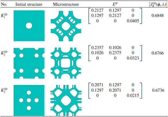
In this section, the prescribed target volume fraction constraint is set to 50%. To investigate the influence of the initial structure on the stability of boundary evolution and the final topological configuration, three representative initial configurations are selected in this study: (1) a central single-hole configuration; (2) a hole configuration with combined boundary and internal distributions; and (3) a central multi-hole configuration. The optimisation results for bulk modulus maximisation are shown in Table 1.
For the evolutionary designs based on the above three different initial structures, this section systematically characterises their topological layouts and macroscopic effective elastic tensors. The corresponding convergence histories of the objective function and volume fraction are shown in Fig. 5.
Optimisation results of the TSBE method for maximising the effective bulk modulus under different initial structures

Table 1. Long description
A table comparing initial structures, microstructures, and effective bulk modulus for different configurations. The table has three rows and four columns. The columns are labeled as No., Initial structure, Microstructure, E H, and J K superscript 2 D. The rows are labeled as K 1 superscript 2 D, K 2 superscript 2 D, and K 3 superscript 2 D. Each row contains the initial structure image, microstructure image, E H matrix values, and J K superscript 2 D value. Row 1: K 1 superscript 2 D, initial structure image with a central single-hole configuration, microstructure image with a complex pattern, E H matrix values [0.2127, 0.1297,"0", 0.1297, 0.2127,"0","0","0", 0.0405], J K superscript 2 D value 0.6848. Row 2: K 2 superscript 2 D, initial structure image with a hole configuration with combined boundary and internal distributions, microstructure image with a complex pattern, E H matrix values [0.2357, 0.1026,"0", 0.1026, 0.2375,"0","0","0", 0.0323], J K superscript 2 D value 0.6766. Row 3: K 3 superscript 2 D, initial structure image with a central multi-hole configuration, microstructure image with a complex pattern, E H matrix values [0.2071, 0.1297,"0", 0.1297, 0.2071,"0","0","0", 0.0215], J K superscript 2 D value 0.6736.", "EDH": "E H matrix values are provided for each configuration.
Convergence histories of the two-dimensional effective bulk modulus for different initial structures: (a)–(c) correspond to initial structures 1, 2 and 3, respectively.

3.1.2 Design for maximising the effective shear modulus
This subsection aims to maximise the effective shear modulus of microstructures. Based on the Voigt mapping rule defined above, the objective function
 $J_G^{2\text{D}}$
is defined as:
 \begin{align} J_G^{2\text{D}}(\boldsymbol{\phi} ,\lambda ) = E_{33}^{\text{H}} \end{align}
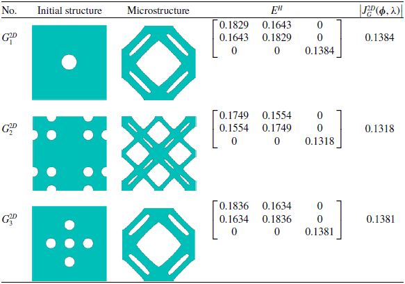
In this example, the prescribed target volume fraction constraint is set to 50%. To maintain consistency in the study and further verify the numerical stability of the algorithm under different mechanical loading conditions, the initial structural configurations selected in this section are identical to those used in the preceding bulk modulus optimisation example. The optimised topological configurations for shear modulus maximisation and the corresponding performance parameters are shown in Table 2.
Optimisation results of the TSBE method for maximising the shear modulus under different initial structures

Table 2. Long description
A table comparing optimization results for shear modulus under different initial structures. The table has four rows and five columns. The columns are labeled No., Initial structure, Microstructure, E H, and J G 2 D (phi, lambda). The rows are labeled G 1 2 D, G 2 2 D, and G 3 2 D. Each row contains an initial structure image, a microstructure image, a 3x3 matrix of values, and a single value. Row 1: G 1 2 D, Initial structure image, Microstructure image, E H matrix [0.1829, 0.1643, 0; 0.1643, 0.1829, 0; 0,"0", 0.1384], J G 2 D (phi, lambda) value 0.1384. Row 2: G 2 2 D, Initial structure image, Microstructure image, E H matrix [0.1749, 0.1554, 0; 0.1554, 0.1749, 0; 0,"0", 0.1318], J G 2 D (phi, lambda) value 0.1318. Row 3: G 3 2 D, Initial structure image, Microstructure image, E H matrix [0.1836, 0.1634, 0; 0.1634, 0.1836, 0; 0,"0", 0.1381], J G 2 D (phi, lambda) value 0.1381.", "EDH": "
For the evolutionary designs based on the above three different initial structures, this section systematically characterises their topological layouts and macroscopic effective elastic tensors. The corresponding convergence histories of the objective function and volume fraction are shown in Fig. 6.
Convergence histories of the two-dimensional effective shear modulus for different initial structures: (a)–(c) correspond to initial structures 1, 2 and 3, respectively.

3.1.3 Benchmarking against theoretical property bounds and analysis of initial-value robustness
To further verify the effectiveness of the TSBE method proposed in this study for microstructural unit-cell configuration optimisation, this section provides an in-depth discussion from the perspectives of physical mechanism and numerical robustness. In the field of two-dimensional topology optimisation and metamaterial design, the theoretical Hashin–Shtrikman (HS) upper bound [Reference Hashin and Shtrikman42] is widely recognised as the theoretical upper limit for macroscopically isotropic solid–void composites at a prescribed volume fraction. By calculating the HS upper-bound attainment ratios of the effective modulus results under different initial conditions, this analysis aims to evaluate the configuration performance from the perspective of the energy principle and to assess the overall mechanical performance of the optimised configurations and the numerical consistency of the proposed framework.
Considering that the classical Hashin–Shtrikman scalar bounds are mainly formulated for macroscopically isotropic effective moduli, this study calculates the attainment ratios relative to the HS upper bound only for the two-dimensional and three-dimensional configurations optimised for maximum bulk modulus. For the configurations optimised for maximum shear stiffness, the target shear stiffness components cannot be strictly equated with the isotropic effective shear modulus defined in the classical HS theory, because the corresponding material distributions exhibit directional characteristics. Therefore, the HS upper-bound attainment ratio for the shear modulus is not defined in this study. In this study, the Young’s modulus of the base material
 ${E_0}$
is set to 1, and the Poisson’s ratio
 ${\upsilon _0}$
is set to 0.3. For a two-dimensional isotropic material composed of a single-phase base material and zero-modulus voids, the theoretical upper bounds of the effective bulk modulus
 $K_{HS,2D}^{up}$
is calculated as follows:
 \begin{align} K_{HS,2D}^{up} = \frac{{V \cdot {K_S} \cdot {G_S}}}{{(1 - V){K_S} + {G_S}}} \end{align}
For a bulk-modulus-optimised configuration, the effective bulk modulus is evaluated as:
 \begin{align} K_{eff}^{2D} = ({E_{11}} + {E_{12}} + {E_{21}} + {E_{22}})/4 \end{align}
The evolutionary path of a structure is generally sensitive to the initial distribution. To evaluate the dependence of the threshold-shift evolution on the initial topology and its ability to handle complex topological reconfiguration, three initial structures with distinctly different spatial characteristics are selected in this section for comparative investigation. By tracking the boundary evolution trajectories under different initial conditions, this study aims to systematically evaluate the numerical stability of the algorithm.
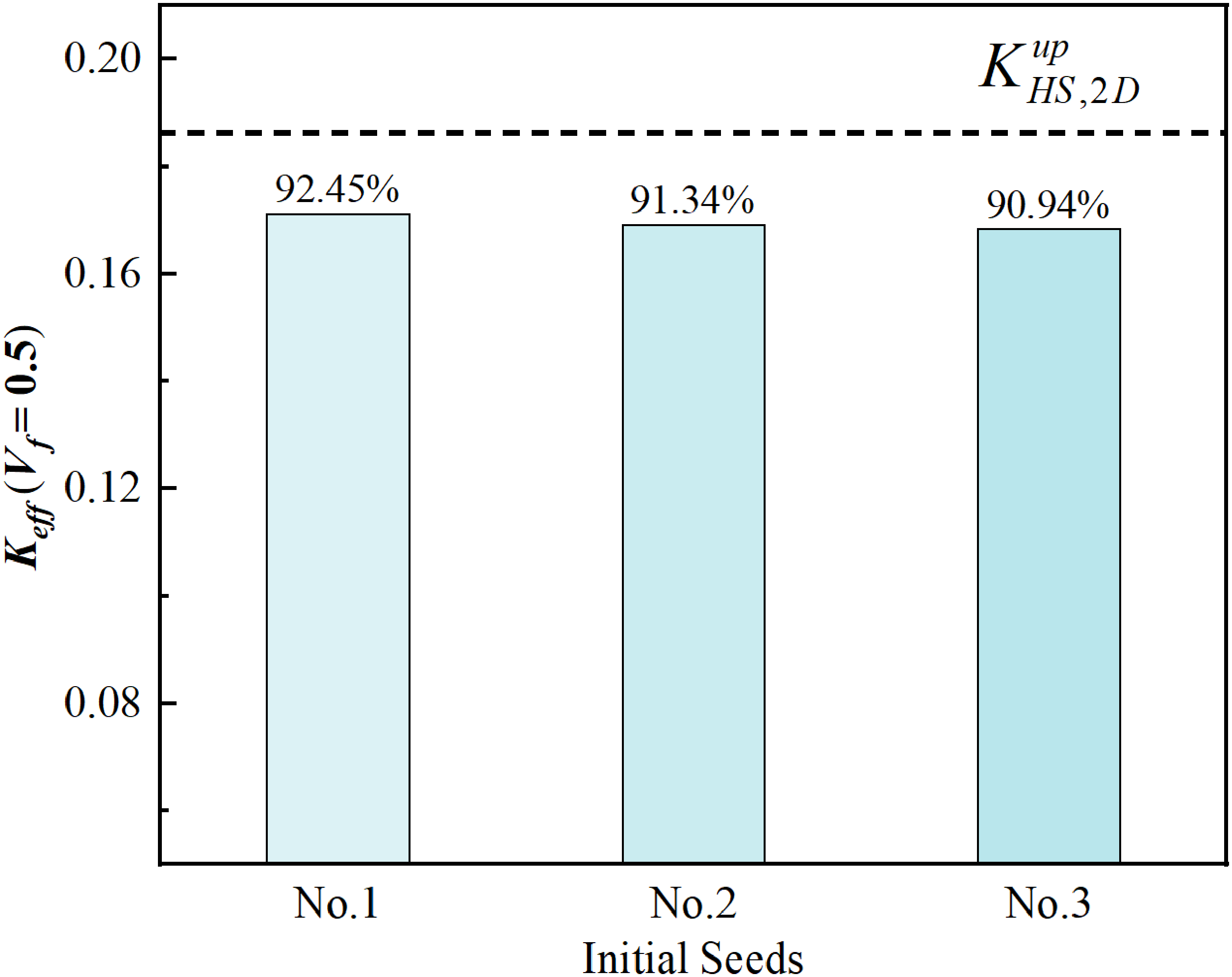
The computational results are shown in Fig. 7. The optimisation processes for the three types of initial configurations show consistent convergence. For the configurations aimed at maximising the bulk modulus, the HS upper-bound attainment ratios are 92.45%, 91.34% and 90.94%, respectively. It is found that, although the final optimised topological configurations exhibit minor microscopic differences in geometric details due to the influence of the initial structural distribution, their equivalent uniform-strain bulk moduli show a high degree of consistency and remain close to the HS bulk-modulus upper bound. This indicates that the proposed algorithm has low sensitivity to the initial topology and demonstrates numerical robustness.
Comparison of two-dimensional bulk-modulus-optimised configurations and their HS bulk-modulus upper-bound attainment ratios.

For the benchmark comparison with the SIMP method, the same initial structures, volume fraction constraint and periodic boundary conditions as those used in the TSBE method are adopted to ensure fairness. The volume fraction is set to 0.5, and the design domain is discretised using a 100 × 100 mesh. Material interpolation is performed using the standard SIMP interpolation model [Reference Bendsøe and Sigmund38]:
 \begin{align} E(\rho ) = {E_{\min }} + {\rho ^p}({E_0} - {E_{\min }}) \end{align}
where
 ${E_0} = 1$
,
 ${E_{\min }} = {10^{ - 9}}$
and the penalisation coefficient
 $p = 3$
are used. During the optimisation process, no penalisation continuation strategy is adopted, and the penalisation coefficient remains constant throughout the iterations. To suppress checkerboard patterns and reduce mesh dependency, a density filtering method is employed [Reference Sigmund39], with the filter radius set to five elements. The optimality criteria method is used as the optimiser, the move limit is set to 0.2 and the design variables are updated using a bisection search for the Lagrange multiplier. The optimisation convergence criterion is determined based on the maximum change in the design variables, denoted as change. For the maximum bulk modulus optimisation example, convergence is considered to be achieved when the maximum change is less than 0.01. For the maximum shear modulus optimisation example, convergence is considered to be achieved when change is less than 0.001. The above SIMP implementation parameters and convergence criteria are set with reference to Ref. (Reference Xia and Breitkopf34). The periodic boundary conditions used in the SIMP method are consistent with those adopted in the proposed method.
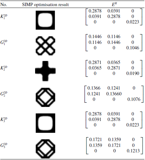
For comparison with the proposed optimisation algorithm, the optimisation results obtained by the SIMP method under the corresponding three different initial structures are considered. By calculating the attainment ratios relative to the HS upper bound for the bulk modulus, the SIMP results are found to be 88.26%, 87.37% and 88.26%, respectively. In this group of examples, the proposed algorithm achieves higher upper-bound attainment ratios than the SIMP method. The computational results are shown in Table 3. Furthermore, because the SIMP method employs density filtering and a penalisation coefficient, grey elements are generated. As a result, the effective elastic model of the SIMP method may be affected by these grey, or intermediate-density, elements, which can lead to relatively lower HS upper-bound attainment ratios. In summary, the comparison results indicate that the TSBE method exhibits good physical consistency in two-dimensional structural performance optimisation and, in this group of examples, achieves higher HS upper-bound attainment ratios together with clearer boundary representation.
Optimisation results of the SIMP method under different initial structures and benchmarking against theoretical limits

Table 3. Long description
A table titled ‘Optimisation results of the SIMP method under different initial structures and benchmarking against theoretical limits’ with six rows and three columns. The columns are labeled ‘No.’, ‘SIMP optimisation result’, and ‘E H superscript H’. The table presents optimization results for different initial structures and their corresponding E H superscript H values. Row 1: No. K 2 D subscript 1, SIMP optimisation result shows a square with a circular cutout, E H superscript H values are 0.2878, 0.0391, 0, 0.0391, 0.2878, 0, 0, 0, 0.0223. Row 2: No. G 2 D subscript 1, SIMP optimisation result shows a cross shape, E H superscript H values are 0.1446, 0.1146, 0, 0.1146, 0.1446, 0, 0, 0, 0.1046. Row 3: No. K 2 D subscript 2, SIMP optimisation result shows a plus sign, E H superscript H values are 0.2871, 0.0365, 0, 0.0365, 0.2871, 0, 0, 0, 0.0190. Row 4: No. G 2 D subscript 2, SIMP optimisation result shows a diamond shape, E H superscript H values are 0.1366, 0.1241, 0, 0.1241, 0.1366, 0, 0, 0, 0.1076. Row 5: No. K 2 D subscript 3, SIMP optimisation result shows a square with a circular cutout, E H superscript H values are 0.2878, 0.0391, 0, 0.0391, 0.2878, 0, 0, 0, 0.0223. Row 6: No. G 2 D subscript 3, SIMP optimisation result shows a diamond shape, E H superscript H values are 0.1721, 0.1359, 0, 0.1359, 0.1721, 0, 0, 0, 0.1213.
3.2 Optimisation of three-dimensional microstructural unit cells for extreme functional properties
In this section, the TSBE method is applied to the topology optimisation design of three-dimensional microstructures with extremal properties as the objective functions. The study focuses on two typical cases: maximising the effective bulk modulus and maximising the effective shear modulus. By introducing different initial structures, the influence of the initial configuration on the evolutionary path of the algorithm, numerical stability and the final optimised topology is investigated in depth.
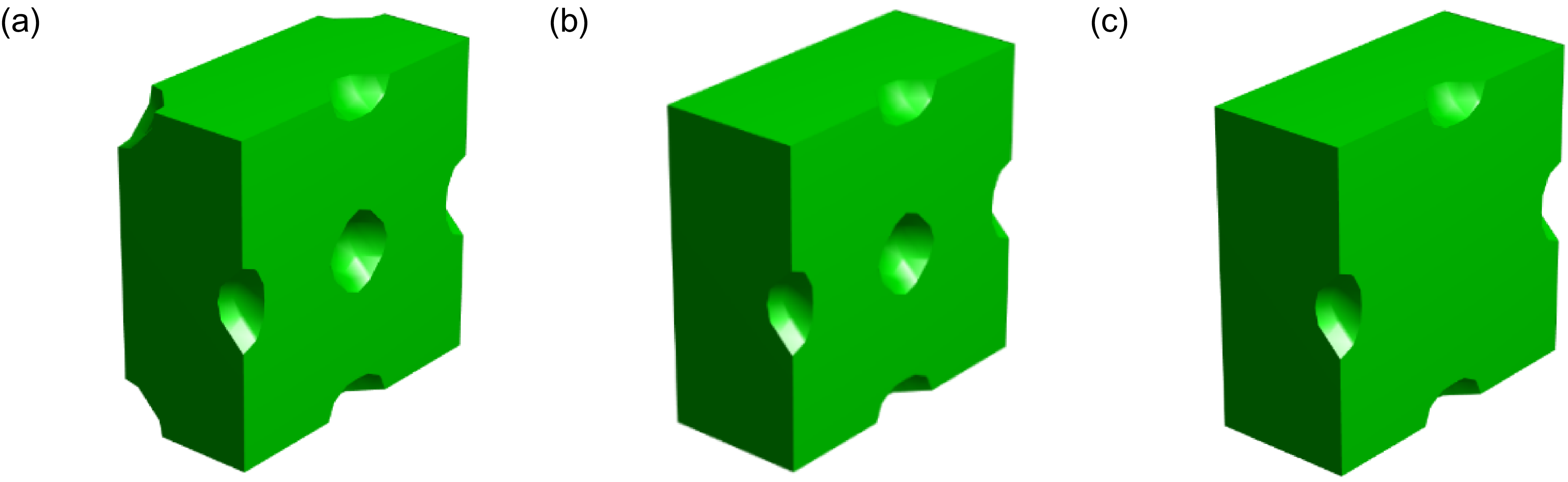
During the numerical optimisation process, the threshold-shift updating mechanism of TSBE established above is adopted. The mesh size of the examples is set to 20 × 20 × 20, and the Poisson’s ratio of the base material is taken as 0.3. The convergence criterion is defined such that the absolute difference between the objective function values of two consecutive iterations is less than 5 × 10⁻⁵, or the maximum number of iterations reaches 150. To verify the robustness of the algorithm, three initial structures with different symmetry characteristics are selected in this section, as shown in Fig. 8: (1) holes distributed at the unit-cell vertices, face centres and body centre; (2) holes distributed at the face centres and body centre; and (3) holes distributed only at the face centres.
Cross-sections of the initial structures: (a)–(c) three-dimensional initial structures with different hole configurations, with holes located at the unit-cell vertices, face centres and body centre in (a), at the face centres and body centre in (b), and at the face centres in (c).

3.2.1 Design for maximising the effective bulk modulus
This example aims to optimise a three-dimensional microstructural configuration with maximum effective bulk modulus. Based on the Voigt mapping rule and the threshold-shift evolutionary framework established above, the objective function
 $J_K^{3\text{D}}$
is defined as:
 \begin{align} J_K^{3\text{D}}(\boldsymbol{\phi},\lambda ) = \sum\limits_{a,b \in \left\{ {1,2,3} \right\}} {E_{ab}^{\text{H}}} = \big(E_{11}^{\text{H}} + E_{22}^{\text{H}} + E_{33}^{\text{H}}\big) + 2\big(E_{12}^{\text{H}} + E_{13}^{\text{H}} + E_{23}^{\text{H}}\big) \end{align}
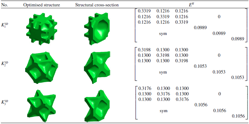
The target volume fraction is set to 50%. Initial structures with different spatial symmetry characteristics are selected to examine their effects on numerical convergence stability, topological evolution paths and final configuration performance under the TSBE threshold-shift updating mechanism. The optimisation results for three-dimensional bulk modulus maximisation are shown in Table 4.
Optimisation results of the TSBE method for maximising the bulk modulus under different initial structures

Table 4. Long description
Table with three columns and multiple rows. The first column is labeled ‘No.’ and contains numerical values. The second column is labeled ‘Optimised structure’ and contains various structural identifiers. The third column is labeled ‘Structural cross-section’ and contains images of cross-sections of different structures. The table presents the results of optimizing the bulk modulus using the TSBE method under different initial structures.
For the evolutionary designs based on the above three different initial structures, this section systematically characterises their topological layouts, macroscopic effective elastic tensors and effective bulk modulus values. The corresponding convergence histories of the objective function and volume fraction are shown in Fig. 9.
Iterative process for three-dimensional bulk modulus maximisation: (a)–(c) show the iterative histories of bulk-modulus-maximisation design starting from 3D initial structures 1, 2 and 3, respectively.

3.2.2 Design for maximising the effective shear modulus
This example aims to optimise a three-dimensional microstructural configuration with maximum effective shear modulus. Based on the Voigt mapping rule and the threshold-shift evolutionary framework established above, the objective function
 $J_G^{3\text{D}}$
is defined as:
 \begin{align} J_G^{3\text{D}}(\boldsymbol{\phi},\lambda ) = \sum\limits_{a \in \left\{ {4,5,6} \right\}} {E_{ab}^{\text{H}}} = E_{44}^{\text{H}} + E_{55}^{\text{H}} + E_{66}^{\text{H}} \end{align}
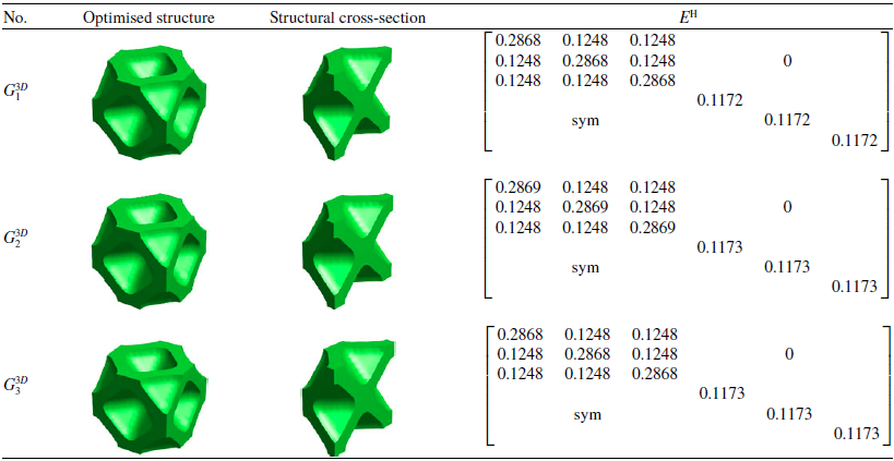
In this example, the prescribed target volume fraction constraint is set to 50%. To maintain consistency in the study and further verify the numerical stability of the algorithm under different mechanical loading conditions, the initial structural configurations selected in this section are identical to those used in the preceding bulk modulus optimisation example. The topological configurations for three-dimensional shear modulus maximisation and the corresponding performance parameters are shown in Table 5.
Optimisation results of the TSBE method for maximising the shear modulus under different initial structures

Table 5. Long description
A table comparing optimized structures and their cross-sections for shear modulus maximization. The table has three rows and four columns. The columns are labeled ‘No.’, ‘Optimised structure’, ‘Structural cross-section’, and ‘E^h’. The rows are labeled with K_1^3D, K_2^3D, and K_3^3D respectively. Each row contains images of the optimized structure and its cross-section, along with a matrix of values. Row 1: K_1^3D, Optimised structure image, Structural cross-section image, E^h matrix with values 0.3319, 0.1216, 0.1216, 0.1216, 0.3319, 0.1216, 0.1216, 0.1216, 0.3319, 0, 0.0989, 0, 0.0989, 0.0989. Row 2: K_2^3D, Optimised structure image, Structural cross-section image, E^h matrix with values 0.3198, 0.1300, 0.1300, 0.1300, 0.3198, 0.1300, 0.1300, 0.1300, 0.3198, 0, 0.1053, 0, 0.1053, 0.1053. Row 3: K_3^3D, Optimised structure image, Structural cross-section image, E^h matrix with values 0.3176, 0.1300, 0.1300, 0.1300, 0.3176, 0.1300, 0.1300, 0.1300, 0.3176, 0, 0.1056, 0, 0.1056, 0.1056.
The above three initial structures are optimised to obtain their microstructural layouts, homogenised elastic tensors and shear modulus values. The corresponding iterative processes are shown in Fig. 10.
Iterative process for three-dimensional shear modulus maximisation: (a)–(c) show the iterative histories of shear-modulus-maximisation design starting from 3D initial structures 1, 2 and 3, respectively.

3.2.3 Verification Against Theoretical Property Bounds and Analysis of Numerical Convergence
At the three-dimensional spatial scale, the macroscopic properties of isotropic porous materials are subject to more stringent constraints imposed by energy principles. For a three-dimensional isotropic unit cell composed only of a single-phase solid matrix and zero-modulus voids, the theoretical HS upper bound of the effective bulk modulus
 $K_{HS,3D}^{up}$
is calculated using the following formula:
 \begin{align} K_{HS,3D}^{up} = \frac{{4{G_0}{K_0}V}}{{4{G_0} + 3{K_0}(1 - V)}} \end{align}
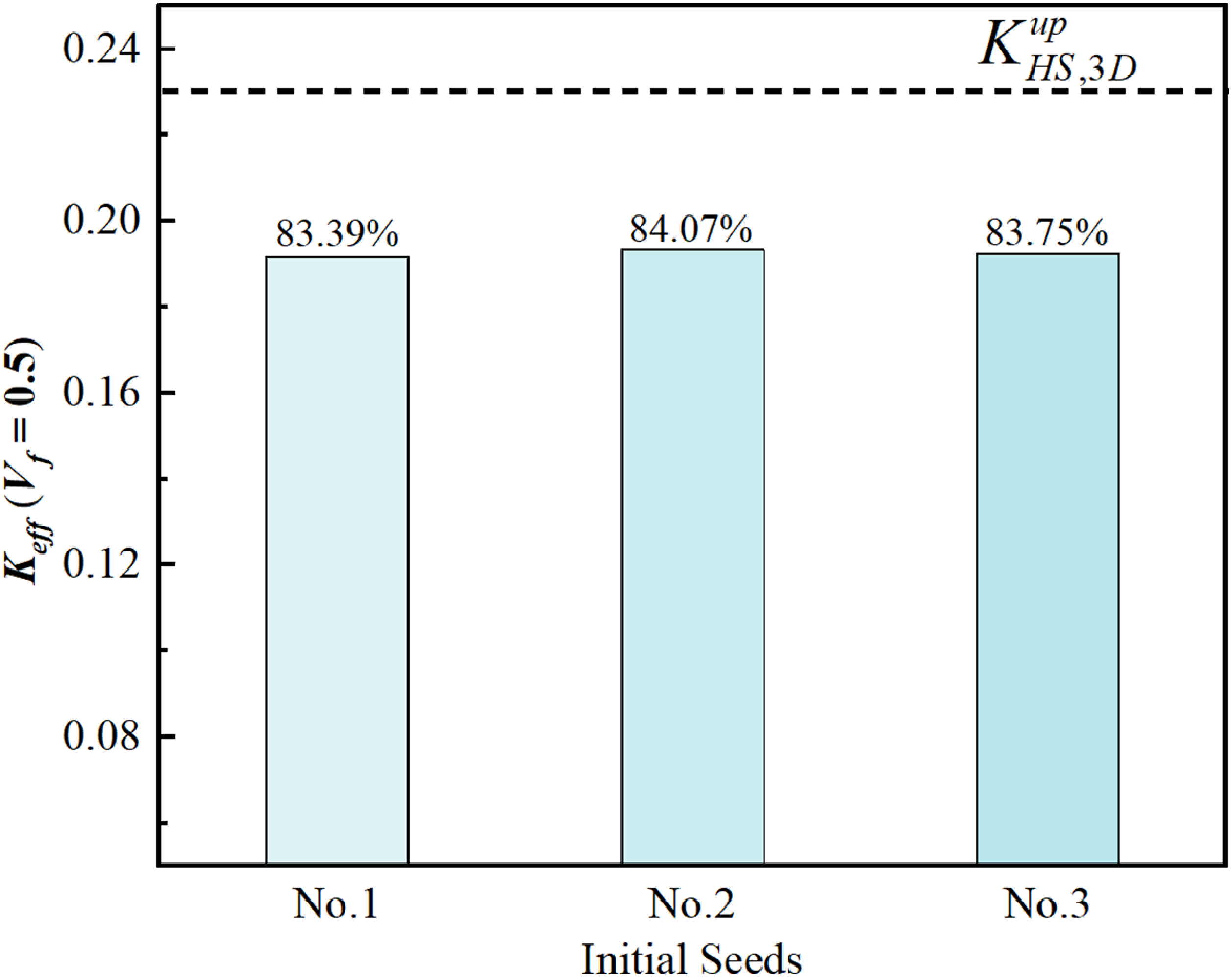
In the three-dimensional microstructural optimisation experiments, this section evaluates the HS bulk-modulus upper-bound attainment ratios only for the configurations optimised for maximum bulk modulus by performing evolutionary optimisation on three initial structures with different spatial characteristics, as shown in Fig. 11. The numerical results show that, under the prescribed volume fraction constraint of 0.5, the HS upper-bound attainment ratios for bulk modulus optimisation are 83.39%, 84.07% and 83.75%. This high convergence consistency indicates that the proposed mechanism exhibits good numerical stability and an effective ability to control sensitivity to the initial conditions in this three-dimensional example.
Comparison of three-dimensional bulk-modulus-optimised configurations and their HS bulk-modulus upper-bound attainment ratios.

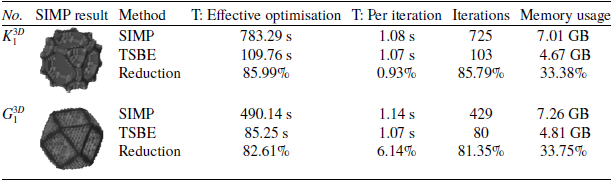
To quantitatively evaluate the computational efficiency of the TSBE method proposed in this study, Initial Structure 1 is selected in this section as a representative example. Under the same mechanical conditions, volume fraction constraint, periodic boundary conditions and convergence criteria, the TSBE method is compared with the conventional SIMP method. The material interpolation model adopted in the SIMP method is given in Equation (39). To ensure a fair comparison of computational time, the effective optimisation time is used for comparison in this study. Specifically, only the time consumed by the core optimisation procedures is counted, including finite element homogenisation calculations, effective stiffness matrix and sensitivity calculations and design-variable updating. Additional time associated with plotting, result saving and other non-optimisation procedures is excluded. The optimisation results and computational efficiency comparison of Initial Structure 1 under maximum bulk modulus optimisation and maximum shear modulus optimisation are shown in Table 6.
Optimisation results and computational efficiency comparison for Initial Structure 1

Table 6. Long description
Table with two rows and seven columns comparing optimization results and computational efficiency for Initial Structure 1. The columns are labeled as No., SIMP result, Method, T: Effective optimization, T: Per iteration, Iterations, and Memory usage. The table presents data for two optimization scenarios: maximum bulk modulus and maximum shear modulus. For maximum bulk modulus optimization, the SIMP method took 783.29 seconds with 725 iterations and 7.01 GB memory usage, while the TSBE method took 109.76 seconds with 103 iterations and 4.67 GB memory usage, showing reductions of 85.99%, 0.93%, 85.79%, and 33.38% respectively. For maximum shear modulus optimization, the SIMP method took 490.14 seconds with 429 iterations and 7.26 GB memory usage, while the TSBE method took 85.25 seconds with 80 iterations and 4.81 GB memory usage, showing reductions of 82.61%, 6.14%, 81.35%, and 33.75% respectively.
Under the two different optimisation objectives, the TSBE method demonstrates high computational efficiency. For the maximum bulk modulus optimisation example, the effective optimisation time of the TSBE method is reduced from 783.29 s for the SIMP method to 109.76 s, corresponding to a reduction of 85.99%. The number of iterations is reduced from 725 to 103, corresponding to a reduction of 85.79%. The memory usage is reduced from 7.01 to 4.67 GB, corresponding to a reduction of 33.38%. For the maximum shear modulus optimisation example, the effective optimisation time of the TSBE method is reduced from 490.14 to 85.25 s, corresponding to a reduction of 82.61%. The number of iterations is reduced from 429 to 80, corresponding to a reduction of 81.35%. The memory usage is reduced from 7.26 to 4.81 GB, corresponding to a reduction of 33.75%.
Meanwhile, the difference in the average time per iteration between the two methods is relatively small. In the maximum bulk modulus optimisation, the average time per iteration is only reduced from 1.08 to 1.07 s when using the TSBE method. In the maximum shear modulus optimisation, the average time per iteration is reduced from 1.14 to 1.07 s. This indicates that the reduction in effective optimisation time is not primarily attributable to a lower per-iteration computational cost, but mainly to fewer iterations and the boundary updating strategy.
In terms of the attainment ratio relative to the HS upper bound for the bulk modulus, the SIMP-optimised Structure 1 achieves 69.03%, which is lower than the 83.39% obtained by the TSBE method. From the perspective of the optimisation results, the SIMP method describes the structure based on an element-density field, leading to a certain number of intermediate-density elements and pixelated boundaries in the optimised configurations. In contrast, the TSBE method describes structural boundaries using a nodal topological potential field and global threshold shifting, which yields clearer and more continuous geometric boundaries and facilitates subsequent structural modeling and manufacturing translation. In summary, under the same optimisation conditions, the TSBE method produces three-dimensional microstructural configurations with clearer boundaries while requiring less computational time and memory, indicating advantages in computational efficiency and geometric representation.
4.0 Application of the threshold-shift boundary evolution method in functional core optimisation
4.1 Functional core design problem and objective formulation
Sandwich structures are commonly used load-bearing forms in lightweight structures such as aerospace components. By integrating the excellent bending resistance of high-strength face sheets with the shear load-carrying capacity of lightweight core materials, such structures can achieve high specific strength and specific stiffness at very low densities. In aerospace service environments, sandwich structures not only effectively combine the high-strength advantages of composite materials, but their porous core layers also exhibit favourable energy absorption and fatigue resistance. Therefore, they can meet the special requirements for vibration suppression and impact resistance in components such as airborne radomes and sound- and heat-insulating fuselage bulkheads.
In practical aerospace engineering, the microscopic topology of the core layer significantly affects the load-bearing efficiency and failure modes of sandwich structures. In launch vehicle fairings or high-performance unmanned aerial vehicle wing spars, core materials are often subjected to complex multiaxial stress states. In particular, under strong shear loads, conventional honeycomb configurations are prone to cell-wall buckling or face-sheet delamination caused by insufficient shear stiffness. Therefore, customised topology optimisation of core materials under multiaxial loading conditions has practical engineering significance.
This section aims to use the proposed TSBE method to design a lightweight core material suitable for multiaxial load-bearing requirements. The objective function is defined as a weighted combination of the uniaxial normal component and the averaged shear components, thereby considering both normal supporting stiffness and multidirectional shear response. The objective function is expressed as:
 \begin{align} {J_{\text{core}}}(\boldsymbol{\phi},\lambda ) = E_{11}^{\text{H}} + w\sum\limits_{a \in \left\{ {4,5,6} \right\}} {E_{aa}^{\text{H}}} = E_{11}^{\text{H}} + \big(E_{44}^{\text{H}} + E_{55}^{\text{H}} + E_{66}^{\text{H}}\big)/3 \end{align}
In the present core-design example, the weighting coefficient is set to
 $w = \frac{1}{3}$
, so that the three orthogonal shear components contribute through their arithmetic mean. The
 $E_{11}^{\text{H}}$
term is introduced to enhance the supporting stiffness of the core material along the primary load-bearing direction, namely the sandwich thickness direction. When the face sheets are subjected to compression, or when the overall structure undergoes bending, the core material helps improve the supporting stiffness in the primary load-bearing direction, thereby preventing local wrinkling or unstable collapse of the face sheets. By maximising this term, the algorithm promotes continuous through-thickness longitudinal load-transfer paths.
Meanwhile, the equally weighted sum of
 $E_{44}^{\text{H}}$
,
 $E_{55}^{\text{H}}$
and
 $E_{66}^{\text{H}}$
is introduced to improve the mean stiffness over the three orthogonal shear cases. Equal weighting assigns the same importance to the three shear planes, but does not enforce equality among their stiffnesses or strict shear isotropy; the optimised core may therefore remain anisotropic. In conventional structures such as hexagonal honeycombs, the stiffness distribution in in-plane and out-of-plane shear planes is often highly nonuniform. Under complex loads such as oblique impact or multiaxial vibration, weak shear performance may induce delamination failure between the face sheets and the core material. In this study, a weighting coefficient is used to average the stiffnesses of the three orthogonal shear planes. This averaging strategy is intended to avoid neglecting any of the three shear planes and to improve their overall shear response. The resulting optimisation strategy drives the structural boundary to generate spatially inclined supporting paths during the evolution process, enabling the force flow to be more evenly distributed in three-dimensional space and forming relatively continuous oblique load-transfer paths.
4.2 Mesh-resolution convergence assessment and HS-referenced performance assessment
4.2.1 Discretisation accuracy verification and mesh-resolution sensitivity analysis
In the implementation, Initial Structure 1, which has a symmetric initial geometry and relatively balanced shear-stiffness components, is selected as the evolutionary baseline. To verify the stability of the algorithm in solving for special properties, 20 × 20 × 20 and 30 × 30 × 30 meshes are adopted to validate the computational results of Initial Structure 1 at volume fractions of 50%, 45%, 40%, 35% and 30%, respectively. The computational results are shown in Fig. 12.
Mesh-resolution convergence assessment and mechanical-performance evaluation of the TSBE-optimized configurations.

To systematically assess the mesh-resolution sensitivity and numerical robustness of the algorithm, this section compares and analyses the configuration evolution results under the two mesh resolutions of
 ${20^3}$
and
 ${30^3}$
over the volume fraction range of 50%, 45%, 40%, 35% and 30%. Data monitoring shows that, as the volume fraction increases stepwise, the primary stiffness component
 $E_{11}^{\text{H}}$
, the mean shear component
 $G_{avg}^{\text{H}}$
and the objective function
 ${J_{\text{core}}}(\phi ,\lambda )$
all exhibit highly synchronised monotonic increasing trends under different mesh densities. Quantitative analysis indicates that the numerical deviations between the two mesh resolutions are relatively small. Taking the volume fraction of 50% as an example, the relative deviation of the objective function values corresponding to the
 ${20^3}$
and
 ${30^3}$
meshes is only 2.62%. Even under the 30% volume fraction condition, where the structure becomes more slender, the deviation in the objective function is effectively controlled within 8%.
In terms of topological morphology evolution, the microstructural configurations obtained under different mesh resolutions exhibit a high degree of geometric consistency, without mesh-resolution-dependent topological distortion or fragmented branches. The evolution process shows a pronounced adaptive wall-thickness characteristic. The topological skeleton of the structure exhibits good stability at the early stage of evolution. As the volume fraction changes, the configuration boundary undergoes approximately normal movement driven by threshold shifting, thereby realising adaptive adjustment of the wall thickness. This phenomenon of morphological fidelity and performance convergence indicates that the subgrid sampling mapping can help reduce the influence of finite element discretisation errors, providing a reference for subsequent parametric design and manufacturing evaluation.
4.2.2 HS-referenced assessment of equivalent uniform-strain moduli
To further evaluate the performance of the proposed algorithm in microstructural design, this section compares the equivalent uniform-strain moduli of the optimised microstructures with the classical isotropic HS upper-bound values used as references [Reference Hashin and Shtrikman42]. Based on the preceding mesh-resolution sensitivity analysis, a high-resolution 303 mesh is adopted in this part for refined characterisation. This analysis extracts the equivalent uniform-strain bulk and shear moduli from the homogenised elastic matrix and reports their ratios to the corresponding isotropic HS reference values.
 \begin{align} K_{{\rm{core}}}^{{\rm{US}}} = \frac{{E_{11}^{\text{H}} + E_{22}^{\text{H}} + E_{33}^{\text{H}} + 2\big(E_{12}^{\text{H}} + E_{13}^{\text{H}} + E_{23}^{\text{H}}\big)}}{9}\nonumber \\[-28pt] \end{align}
 \begin{align} G_{{\rm{core}}}^{{\rm{US}}} = \frac{{E_{44}^{\text{H}} + E_{55}^{\text{H}} + E_{66}^{\text{H}}}}{3} \end{align}
Here
 $K_{{\rm{core}}}^{{\rm{US}}}$
and
 $G_{{\rm{core}}}^{{\rm{US}}}$
denote the equivalent uniform-strain bulk modulus and the equivalent uniform-strain shear modulus extracted from the homogenised stiffness matrix, respectively. Because the optimised core is generally anisotropic, the classical isotropic HS expressions are used only as reference values. Accordingly,
 $K_{{\rm{core}}}^{{\rm{US}}}/K_{{\rm{HS,3D}}}^{up}$
and
 $G_{{\rm{core}}}^{{\rm{US}}}/G_{{\rm{HS,3D}}}^{up}$
are termed HS-normalised reference ratios rather than rigorous HS-bound attainment ratios.
The computational results, as shown in Fig. 13, indicate that the optimised configurations exhibit high HS-normalised reference ratios within the prescribed range of volume fractions. Specifically, the HS-normalised reference ratio of the equivalent uniform-strain bulk modulus steadily increases from 81.11% at a volume fraction of 0.3 to 86.47% at a volume fraction of 0.5. Meanwhile, the HS-normalised reference ratio of the equivalent uniform-strain shear modulus ranges from 89.42% at a volume fraction of 0.3 to 94.19% at a volume fraction of 0.5. This favourable balance and upward trend in both bulk and shear responses indicate that the algorithm produces relatively balanced bulk/shear performance under the multi-condition composite objective and forms reasonable spatial load-transfer paths.
HS-normalised reference ratios of the equivalent uniform-strain bulk and shear moduli of the TSBE-optimised core on the 30³ mesh.

The HS-normalised reference ratios, together with the mesh-resolution sensitivity results, indicate that the optimised configurations retain substantial equivalent bulk and shear stiffness relative to the corresponding isotropic reference values. These ratios reflect the combined effects of the selected objective function, sensitivity mapping, threshold-shift updating and subgrid projection, and should not be interpreted as proof that the anisotropic cores attain the classical isotropic HS bounds.
4.3 Numerical Validation of the Optimized Structure
The evolutionary study of core structures under different volume fractions shows that this type of configuration exhibits favourable topological robustness and geometric self-similarity. During the stepwise reduction in volume fraction, the microstructural unit cell mainly follows an evolutionary logic of adaptive wall-thickness reduction, while the overall load-transfer skeleton does not undergo substantial abrupt changes. This behaviour indicates that the morphological evolution is dominated by adaptive wall-thickness changes, while the principal load-transfer skeleton remains comparatively stable over the investigated volume-fraction range, providing a reference for subsequent multiscale configuration design.
In terms of geometric representation, the external envelope profile of the lightweight core material remains constant during the evolution process. Material reduction is mainly achieved through the normal expansion of the internal contours, that is, by inducing the formation of internal cavities to reduce the apparent density. Taking the configuration with a volume fraction of 30% as an example, its effective elastic matrix exhibits directional shear enhancement. This result indicates that the objective function has a guiding effect on specific shear responses, while the dominant mechanical characteristics of the corresponding configuration still need to be further evaluated through subsequent finite element benchmarking.
 \begin{align} {\delta _{ij}} = \frac{{2\left| {C_{ij}^{FEA} - C_{ij}^{TO}} \right|}}{{\left| {C_{ij}^{FEA}} \right| + \left| {C_{ij}^{TO}} \right|}} \times 100\% \end{align}
where
 ${\delta _{ij}}$
is the symmetric relative difference of stiffness component
 ${C_{ij}}$
,
 $C_{ij}^{FEA}$
and
 $C_{ij}^{TO}$
denote the corresponding stiffness components obtained from the reconstructed finite element model and the TSBE optimisation model, respectively. Equation (46) is applied component-wise; for the overall stiffness-matrix comparison, the same symmetric relative-difference definition is adopted by replacing the absolute value with the Frobenius norm.
After refinement from FEA-20 to FEA-30, the variations in the major stiffness components are relatively small. Their effective elastic matrices are shown in Table 7. Specifically, the difference in
 ${C_{11}}$
is approximately 0.13%, the difference in the shear-enhanced component
 ${C_{55}}$
is approximately 1.0% and the symmetric relative difference of the overall stiffness matrix is approximately 0.4%. This indicates that the current reconstructed finite element model is insensitive to changes in mesh density, and that the finite element results exhibit good numerical stability.
Comparison between the TSBE method and finite element calculation results

Table 7. Long description
A table comparing optimized structures, structural cross-sections, and effective elastic matrices for three different methods. The table has three rows and four columns. The columns are labeled ‘No.’, ‘Optimised structure’, ‘Structural cross-section’, and ‘E^H’. The rows are labeled ‘G_1^3D’, ‘G_2^3D’, and ‘G_3^3D’. Each row contains images of the optimized structure and structural cross-section, followed by a 3x3 matrix of values and a symmetric value. Row 1: G_1^3D, optimized structure image, structural cross-section image, matrix values [0.2868, 0.1248, 0.1248; 0.1248, 0.2868, 0.1248; 0.1248, 0.1248, 0.2868], symmetric value 0.1172. Row 2: G_2^3D, optimized structure image, structural cross-section image, matrix values [0.2869, 0.1248, 0.1248; 0.1248, 0.2869, 0.1248; 0.1248, 0.1248, 0.2869], symmetric value 0.1173. Row 3: G_3^3D, optimized structure image, structural cross-section image, matrix values [0.2868, 0.1248, 0.1248; 0.1248, 0.2868, 0.1248; 0.1248, 0.1248, 0.2868], symmetric value 0.1173.
Compared with the predictions of the TSBE method, the stiffness components obtained from FEA-30 are generally higher. Based on the symmetric relative difference, the component-wise differences between FEA-30 and the algorithmic results are approximately 7.4–10.2%, while the difference in the overall stiffness matrix is approximately 8.4%. It should be noted that this discrepancy should not be simply attributed to numerical hardening of the finite elements or insufficient mesh density. In the TSBE method, the material boundary is determined on a fixed background mesh based on the nodal topological potential field and the threshold-shift mechanism, and the material occupancy state within boundary elements is calculated through subgrid integration. In contrast, the finite element model requires this implicit boundary representation to be converted into explicit solid geometry. Therefore, even if the overall volume fractions of the two models are nearly identical, subtle differences may still exist in local boundary positions, strut profiles, nodal connection regions and narrow connecting regions. For thin-walled periodic configurations, the effective stiffness is relatively sensitive to these local geometric features. Consequently, the above boundary reconstruction differences may cause the finite element model to predict systematically higher absolute stiffness values than the algorithmic model.
To further distinguish the difference in absolute stiffness magnitude from the difference in intrinsic mechanical characteristics of the configuration, dimensionless normalised mechanical indicators are introduced in this study for supplementary comparison, as shown in Table 8. These normalised indicators are directly constructed from the components of the effective elastic matrix. They mainly reflect the relative proportional relationships among stiffness components rather than the absolute magnitude of any single stiffness component. Therefore, they can be used to evaluate the prediction consistency of the two models in terms of anisotropic distribution, shear-enhancement tendency and transverse coupling behaviour of the configuration.
Comparison of dimensionless stiffness ratios obtained from the TSBE optimisation and reconstructed finite element analyses

Table 8. Long description
A table comparing dimensionless stiffness ratios obtained from the TSBE optimisation and reconstructed finite element analyses. The table has five rows and five columns. The columns are labeled as Difference, Metric, Definition, TSBE, FEA-20, FEA-30, and FEA-30 and TSBE (%). The rows are labeled with different metrics: Shear stiffness enhancement ratio, Poisson-related coupling ratio, Transverse coupling ratio, and Transverse stiffness symmetry ratio. The values in the table are as follows: Row 1: Shear stiffness enhancement ratio, 1.2904, 1.2769, 1.2683, 1.7. Row 2: Poisson-related coupling ratio, 0.1816, 0.1863, 0.1859, 2.3. Row 3: Transverse coupling ratio, 0.9319, 0.9326, 0.9267, 0.6. Row 4: Transverse stiffness symmetry ratio, 1.0000, 1.0030, 1.0060, 0.6.
The results show that, although there is an overall stiffness matrix difference of approximately 8.4% between FEA-30 and the algorithmic prediction, the two models maintain a high degree of consistency in the normalised mechanical indicators. Specifically, the difference in the shear stiffness enhancement ratio
 ${C_{55}}/{C_{44}}$
is approximately 1.7%, the difference in the Poisson-related coupling ratio
 ${C_{12}}/{C_{11}}$
is 2.3%, the difference in the transverse coupling ratio
 ${C_{23}}/{C_{22}}$
is approximately 0.6%, and the difference in the transverse stiffness symmetry ratio
 ${C_{22}}/{C_{33}}$
is approximately 0.6%. This indicates that, although the two models exhibit an offset in absolute stiffness magnitude, their predictions remain consistent in terms of the shear-enhancement direction, transverse coupling characteristics, anisotropic distribution and symmetry patterns of the configuration.
In summary, the comparison between FEA-20 and FEA-30 demonstrates that the current reconstructed finite element model exhibits good numerical stability after mesh refinement. The remaining differences between the FEA and algorithmic results mainly reflect local boundary representation differences between the implicit boundary representation determined by the nodal topological potential field and the explicit finite element geometry, rather than insufficient finite element mesh density or failure of the subgrid projection-mapping mechanism. The consistency of the normalised mechanical indicators further demonstrates that the TSBE method can effectively capture the dominant mechanical response and intrinsic anisotropic characteristics of the optimised configuration.
The relatively small differences in the normalised indicators indicate that, although the absolute stiffness magnitudes exhibit offsets due to differences in numerical integration and geometric reconstruction, the anisotropic distribution patterns and primary load-transfer paths within the configuration remain consistent between the two models. This result further demonstrates that the TSBE method can effectively preserve the dominant mechanical characteristics of the optimised configuration while reducing computational cost.
5.0 Conclusion
This study focuses on the efficient topology optimisation and refined interface representation of lightweight functional core materials. A TSBE method combining a nodal topological potential field, global threshold shifting and subgrid mapping is established. The proposed method is validated through extremal-performance unit cells, sandwich core design and high-fidelity finite element benchmarking. The main conclusions are as follows:
-
(1) A TSBE method jointly driven by a nodal topological potential field and global threshold shifting is constructed. In this framework, a continuous topological potential field is formed through interpolation of nodal variables. By exploiting the monotonicity of the volume-constraint residual with respect to the threshold-shift amount, the threshold position satisfying the volume fraction constraint is determined through bisection search in the scalar threshold space, thereby transforming boundary updating into an algebraic optimisation process. The two- and three-dimensional examples show that this mechanism yields extremal-performance unit cells with consistent convergence under different initial configurations. In the representative three-dimensional examples, compared with the conventional SIMP method, the effective optimisation time is reduced and the memory usage is reduced by 33.38–33.75%, indicating that the proposed method offers computational-efficiency advantages and good numerical stability in this group of examples.
-
(2) The physical mapping mechanism between the continuous topological-potential field and subgrid sampling integration is clarified. Without increasing the finite element degrees of freedom, the material fraction within boundary elements is mapped to equivalent element stiffness parameters, allowing the material–void interface to be represented within the fixed analysis mesh. For the two- and three-dimensional configurations optimised for maximum bulk modulus, the HS bulk-modulus upper-bound attainment ratios range from 83.39% to 92.45%. For the generally anisotropic functional-core configurations, the equivalent uniform-strain bulk and shear moduli reach 81.11–94.19% of the corresponding isotropic HS reference values; these quantities are reported as HS-normalised reference ratios rather than rigorous bound-attainment ratios. The reconstructed finite element models further preserve the dominant normalised mechanical characteristics of the optimised configurations.
-
(3) The boundary evolution patterns of functional core materials for multiaxial load-bearing requirements are revealed. The optimisation results of sandwich-structure core materials show that the proposed method can achieve a coordinated design between the primary supporting stiffness and multidirectional shear resistance. During the configuration evolution process, the topological skeleton stabilises at an early stage, while the subsequent evolution is mainly realised through continuous boundary movement within the fixed analysis mesh driven by threshold shifting, thereby enabling adaptive adjustment of wall thickness with the volume fraction. This geometric self-similar feature of ‘stable skeleton and adaptive wall thickness’ is beneficial for maintaining the continuity of mechanical responses at different material volume fractions and also provides a clear configuration basis for explicit geometric reconstruction and finite element validation.
Competing interests
The authors declare no competing interests.

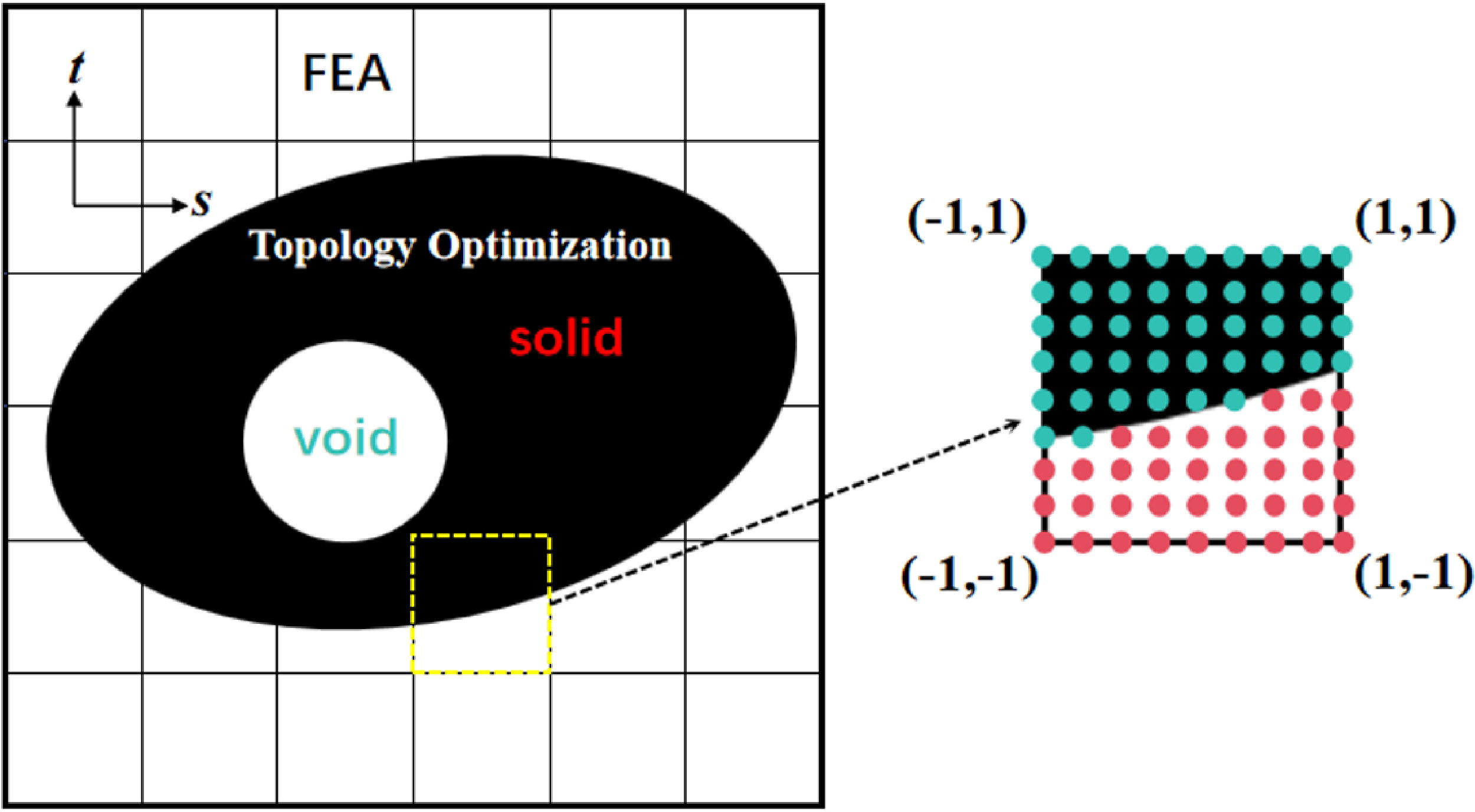

 Ψ≥0
 Ψ<0

 Ψ≥0
 Ψ<0