1 Introduction
The thinning of viscoelastic filaments and the formation of drops are important for many practical applications (Basaran, Gao & Bhat Reference Basaran, Gao and Bhat2013), ranging from the printing of silver pastes for electronics to the deposition of cells for tissue engineering. The development of accurate numerical modelling of viscoelastic flows, including filament thinning and breakup, would provide significant advances to the fundamental understanding of the physics at play and lead to the development of reproducible fabrication techniques.
A theoretical approach to investigate viscoelastic filament thinning has been the use of a slender jet formulation, which is derived using the lubrication approximation (Eggers & Villermaux Reference Eggers and Villermaux2008) coupled with the constitutive equation of the viscoelastic model. This approximation results in a one-dimensional model, consisting of an equation of motion to track the axial velocity component,
 $u_{z}$
, an advection equation to track the filament thickness in the axial direction,
 $h$
, and constitutive equations to track the axial and radial components of the polymeric stress,
 $\unicode[STIX]{x1D70E}_{zz}$
and
 $\unicode[STIX]{x1D70E}_{rr}$
respectively. This one-dimensional description has been used to investigate the thinning of viscoelastic filaments, with a special emphasis given to the thinning of Oldroyd-B and finitely extensible nonlinear elastic (FENE) fluids (Wagner et al.
Reference Wagner, Amarouchene, Bonn and Eggers2005; Clasen et al.
Reference Clasen, Eggers, Fontelos, Li and McKinley2006; Ardekani, Sharma & McKinley Reference Ardekani, Sharma and McKinley2010). The Oldroyd-B constitutive equations have attracted considerable earlier attention because they exhibit the formation of the ‘beads-on-a-string’ structure, which denotes the formation of periodic droplets attached along a filament (Li & Fontelos Reference Li and Fontelos2003). To fully capture this structure, the distribution of stress components in the neck region connecting the thread with the drop should be resolved in detail, which cannot be accomplished using the one-dimensional slender formulation because the structure of drops attached to a thin filament is not slender. Therefore, the complete equations should be simulated in an axially symmetric domain to examine the velocity and stress field throughout the filament.
Simulations of the breakup of a viscoelastic filament in an axially symmetric domain have been presented by Bousfield et al. (Reference Bousfield, Keunings, Marrucci and Denn1986) and Étienne, Hinch & Li (Reference Étienne, Hinch and Li2006), where the problem could be simulated until the minimum filament thickness thinned and reached 50 % and 30 % of the initial radius respectively. The increasing stiffness of the problem prevents the simulation from proceeding further in time because the Oldroyd-B model allows for the buildup of an infinite stress, so that the filament should not break up as long as the numerical grid is sufficiently small. The inkjet printing process motivates the simulation of viscoelastic jets, using a coupled Lagrangian–Eulerian scheme with finite element discretization (Harlen, Rallison & Szabo Reference Harlen, Rallison and Szabo1995; Morrison & Harlen Reference Morrison and Harlen2010) and a constitutive model that allows for breakup such as FENE-P. Like FENE-P, there are other constitutive models that avoid the development of infinite stresses. For instance, the Giesekus model (Hulsen, Fattal & Kupferman Reference Hulsen, Fattal and Kupferman2005) is used to represent shear-thinning polymer solutions, while FENE-CR (Haward et al. Reference Haward, Oliveira, Alves and McKinley2012) is an empirical model that modifies the FENE-P model to separate the shear-thinning effects from the elastic effects.
The complexity of viscoelastic filament thinning comes from the different time scales involved. The time scales to characterize the viscoelastic thinning are the relaxation time,
 $\unicode[STIX]{x1D706}$
, which is the time for the strain to relax when an applied stress is removed, the viscous-capillary time scale,
 $t_{v}=\unicode[STIX]{x1D702}_{0}R_{0}/\unicode[STIX]{x1D6FE}$
, and the inertia-capillary time scale,
 $t_{c}=\sqrt{\unicode[STIX]{x1D70C}R_{0}^{3}/\unicode[STIX]{x1D6FE}}$
, where
 $R_{0}$
is the filament radius,
 $\unicode[STIX]{x1D70C}$
is the density,
 $\unicode[STIX]{x1D6FE}$
is the surface tension with air and
 $\unicode[STIX]{x1D702}_{0}=\unicode[STIX]{x1D702}_{s}+\unicode[STIX]{x1D702}_{p}$
is the zero shear viscosity, with
 $\unicode[STIX]{x1D702}_{s}$
and
 $\unicode[STIX]{x1D702}_{p}$
the solvent and polymeric viscosities respectively. This defines two non-dimensional numbers, the Deborah number,
 $De$
, and the Ohnesorge number,
 $Oh$
(Bhat et al.
Reference Bhat, Appathurai, Harris, Pasquali, McKinley and Basaran2010; Turkoz et al.
Reference Turkoz, Perazzo, Kim, Stone and Arnold2018),
 $$\begin{eqnarray}\displaystyle De=\frac{\unicode[STIX]{x1D706}}{t_{c}}=\frac{\unicode[STIX]{x1D706}}{\sqrt{\unicode[STIX]{x1D70C}R_{0}^{3}/\unicode[STIX]{x1D6FE}}},\quad Oh=\frac{t_{v}}{t_{c}}=\frac{\unicode[STIX]{x1D702}_{0}}{\sqrt{\unicode[STIX]{x1D70C}\unicode[STIX]{x1D6FE}R_{0}}}. & & \displaystyle\end{eqnarray}$$
The Ohnesorge number compares the inertia-capillary and viscous-capillary time scales. The Deborah number compares the fluid relaxation time with the flow time scale and in many cases is equivalent to the Weissenberg number (Dealy Reference Dealy2010),
 $Wi=\unicode[STIX]{x1D706}\dot{\unicode[STIX]{x1D716}}$
, where
 $\dot{\unicode[STIX]{x1D716}}$
is the strain rate. For high-Deborah-number flows, simulations performed with the conventional finite volume discretization of the full set of equations have suffered from the phenomenon called the high-Weissenberg-number problem (Keunings Reference Keunings1986; Renardy Reference Renardy2000). This problem arises when the Oldroyd-B model is used and the stresses inside the filament continue to rise exponentially without a limit. Eventually, the numerical simulations fail in resolving these high stresses and stress gradients (Renardy Reference Renardy2000). Various transformations have been proposed to overcome this challenge, such as the kernel-transformation (Balci et al.
Reference Balci, Thomases, Renardy and Doering2011) and log-conformation (Fattal & Kupferman Reference Fattal and Kupferman2005) techniques. Here, we use the log-conformation technique to overcome the high-Weissenberg-number problem. This technique is based on reformulation of the constitutive equation in terms of the matrix logarithm of the conformation tensor. According to Fattal & Kupferman (Reference Fattal and Kupferman2005), taking the matrix logarithm reduces the exponential variation of the conformation tensor so that this variation can be approximated by polynomials. We also tried to use the kernel-transformation technique to solve for the polymeric stresses; however, this technique did not lead to convergence for our configuration.
The rate of thinning of viscoelastic fluids can be described as the balance of surface tension and elastic forces, with the assumption of a spatially constant and slender profile (Bazilevskii et al.
Reference Bazilevskii, Entov, Lerner and Rozhkov1997). This leads to an exponential decrease of the minimum radius of a thinning viscoelastic filament,
 $h_{min}$
, with time (Clasen et al.
Reference Clasen, Eggers, Fontelos, Li and McKinley2006),
 $$\begin{eqnarray}h_{min}(t)=h_{0}\exp [-t/(3\unicode[STIX]{x1D706})],\end{eqnarray}$$
where
 $h_{0}$
depends on the initial conditions. Equation (1.2) is used to evaluate the relaxation time of viscoelastic fluids from the time evolution of
 $h_{min}$
(Anna & McKinley Reference Anna and McKinley2001). Therefore, an accurate numerical model should capture the exponential polymeric thinning accurately. The axial polymeric stress,
 $\unicode[STIX]{x1D70E}_{zz}$
, and the velocity component can also be derived and are given by Clasen et al. (Reference Clasen, Eggers, Fontelos, Li and McKinley2006) as
 $$\begin{eqnarray}\displaystyle \unicode[STIX]{x1D70E}_{zz}=\unicode[STIX]{x1D70E}_{0}\exp (t/3\unicode[STIX]{x1D706}),\quad \frac{\unicode[STIX]{x2202}u_{z}}{\unicode[STIX]{x2202}z}=\frac{2}{3\unicode[STIX]{x1D706}}, & & \displaystyle\end{eqnarray}$$
where
 $\unicode[STIX]{x1D70E}_{0}$
is the stress value at the beginning of the exponential thinning. Accurate capture of these relationships can be considered as a benchmark for numerical models of viscoelastic fluids.
In this paper, we examine the thinning of an Oldroyd-B type of filament by using direct numerical simulations and solving the axisymmetric two-phase incompressible momentum equations with surface tension using the open source solver Basilisk (Popinet Reference Popinet2015, Reference Popinet2018). The interface between the high-density viscoelastic liquid and the low-density ambient air is reconstructed by a volume-of-fluid (VOF) method, which has been validated for complex multiphase flows such as splashing (Howland et al. Reference Howland, Antkowiak, Castrejón-Pita, Howison, Oliver, Style and Castrejón-Pita2016), breaking waves (Deike, Melville & Popinet Reference Deike, Melville and Popinet2016) and bubble bursting (Deike et al. Reference Deike, Ghabache, Liger-Belair, Das, Zaleski, Popinet and Séon2018). Here, we find that the time evolution of the thinning thread and the axial distribution of velocity and polymeric stress components along the filament follow the theoretical predictions. Moreover, while the one-dimensional approximation can capture the trends of stresses successfully, the off-diagonal stress component of the polymeric stress tensor is not negligible as the thinning progresses in time.
2 Numerical simulations
We consider incompressible mass conservation and momentum equations with the addition of the polymeric stress as an extra term in the stress tensor. These equations are given by Clasen et al. (Reference Clasen, Eggers, Fontelos, Li and McKinley2006) as
 $$\begin{eqnarray}\displaystyle & \unicode[STIX]{x1D735}\boldsymbol{\cdot }\boldsymbol{u}=0, & \displaystyle\end{eqnarray}$$
 $$\begin{eqnarray}\displaystyle & \displaystyle \unicode[STIX]{x1D70C}\left(\frac{\unicode[STIX]{x2202}\boldsymbol{u}}{\unicode[STIX]{x2202}t}+\boldsymbol{u}\boldsymbol{\cdot }\unicode[STIX]{x1D735}\boldsymbol{u}\right)=-\unicode[STIX]{x1D735}p+\unicode[STIX]{x1D735}\boldsymbol{\cdot }\text{}\underline{\text{}\underline{\unicode[STIX]{x1D748}}}, & \displaystyle\end{eqnarray}$$
where the total stress tensor has two components,
 $\text{}\underline{\text{}\underline{\unicode[STIX]{x1D748}}}=\text{}\underline{\text{}\underline{\unicode[STIX]{x1D70E}_{s}}}+\text{}\underline{\text{}\underline{\unicode[STIX]{x1D70E}_{p}}}$
. The solvent viscous stress tensor has the usual definition,
 $\text{}\underline{\text{}\underline{\unicode[STIX]{x1D70E}}}_{s}=2\unicode[STIX]{x1D702}_{s}\text{}\underline{\text{}\underline{\unicode[STIX]{x1D63F}}}$
, where
 $\unicode[STIX]{x1D702}_{s}$
is the solvent viscosity and
 $\text{}\underline{\text{}\underline{\unicode[STIX]{x1D63F}}}=(\unicode[STIX]{x1D735}\boldsymbol{u}+\unicode[STIX]{x1D735}\boldsymbol{u}^{\text{T}})/2$
is the strain-rate tensor. The polymeric stress tensor is evaluated according to the Oldroyd-B model as (Ardekani et al.
Reference Ardekani, Sharma and McKinley2010)
 $$\begin{eqnarray}\frac{\text{D}\text{}\underline{\text{}\underline{\unicode[STIX]{x1D70E}_{p}}}}{\text{D}t}=(\unicode[STIX]{x1D735}\boldsymbol{u})^{\text{T}}\boldsymbol{\cdot }\text{}\underline{\text{}\underline{\unicode[STIX]{x1D70E}_{p}}}+\text{}\underline{\text{}\underline{\unicode[STIX]{x1D70E}_{p}}}\boldsymbol{\cdot }(\unicode[STIX]{x1D735}\boldsymbol{u})-\frac{1}{\unicode[STIX]{x1D706}}\text{}\underline{\text{}\underline{\unicode[STIX]{x1D748}_{p}}}+\frac{\unicode[STIX]{x1D702}_{p}}{\unicode[STIX]{x1D706}}(\unicode[STIX]{x1D735}\boldsymbol{u}+\unicode[STIX]{x1D735}\boldsymbol{u}^{\text{T}}),\end{eqnarray}$$
where
 $\unicode[STIX]{x1D702}_{p}$
is the polymer viscosity and
 $\unicode[STIX]{x1D706}$
is the relaxation time as explained in the previous section. We represent the governing parameters of filament thinning following the study presented by Clasen et al. (Reference Clasen, Eggers, Fontelos, Li and McKinley2006). The total dynamic viscosity of the polymer solution is denoted as
 $\unicode[STIX]{x1D702}_{0}=\unicode[STIX]{x1D702}_{s}+\unicode[STIX]{x1D702}_{p}$
. An important parameter that affects the stiffness of the problem is the viscosity ratio, defined as
 $\unicode[STIX]{x1D6FD}=\unicode[STIX]{x1D702}_{s}/\unicode[STIX]{x1D702}_{0}$
. As the viscosity ratio decreases, the problem becomes numerically more challenging to solve. An alternative and equivalent representation is to separate the relative dimensionless contributions of the viscosity,
 $\unicode[STIX]{x1D708}_{s}=Oh\unicode[STIX]{x1D6FD}$
for the solvent and
 $\unicode[STIX]{x1D708}_{p}=Oh(1-\unicode[STIX]{x1D6FD})$
for the polymer (Clasen et al.
Reference Clasen, Eggers, Fontelos, Li and McKinley2006).
In the log-conformation technique, one solves for the conformation tensor
 $\text{}\underline{\text{}\underline{\unicode[STIX]{x1D658}}}$
instead of the polymeric stress tensor as given in (2.3). In the Oldroyd-B model, these two tensors are related by
 $\text{}\underline{\text{}\underline{\unicode[STIX]{x1D70E}_{p}}}=(\unicode[STIX]{x1D706}/\unicode[STIX]{x1D702}_{p})(\text{}\underline{\text{}\underline{\unicode[STIX]{x1D658}}}-\text{}\underline{\text{}\underline{\unicode[STIX]{x1D644}}})$
, where
 $\text{}\underline{\text{}\underline{\unicode[STIX]{x1D644}}}$
is the identity matrix. Then, the equation for the conformation tensor becomes
 $$\begin{eqnarray}\frac{\unicode[STIX]{x2202}\text{}\underline{\text{}\underline{\unicode[STIX]{x1D658}}}}{\unicode[STIX]{x2202}t}+\boldsymbol{u}\boldsymbol{\cdot }\unicode[STIX]{x1D735}\text{}\underline{\text{}\underline{\unicode[STIX]{x1D658}}}-(\unicode[STIX]{x1D735}\boldsymbol{u}\boldsymbol{\cdot }\text{}\underline{\text{}\underline{\unicode[STIX]{x1D658}}}+\text{}\underline{\text{}\underline{\unicode[STIX]{x1D658}}}\boldsymbol{\cdot }\unicode[STIX]{x1D735}\boldsymbol{u}^{\text{T}})=\frac{1}{\unicode[STIX]{x1D706}}(\text{}\underline{\text{}\underline{\unicode[STIX]{x1D658}}}-\text{}\underline{\text{}\underline{\unicode[STIX]{x1D644}}}).\end{eqnarray}$$
The components of this tensor are solved using the numerical scheme presented by Hao & Pan (Reference Hao and Pan2007) by first taking the matrix logarithm of the conformation tensor as
 $\text{}\underline{\text{}\underline{\unicode[STIX]{x1D74D}}}=\log \text{}\underline{\text{}\underline{\unicode[STIX]{x1D658}}}$
. This is possible because the conformation tensor is always positive definite. The equation for
 $\text{}\underline{\text{}\underline{\unicode[STIX]{x1D74D}}}$
is easier to solve numerically because the logarithm of the exponentially increasing polymeric stresses is resolved. After the equation is solved, the conformation tensor is evaluated as
 $\text{}\underline{\text{}\underline{\unicode[STIX]{x1D658}}}=\exp (\text{}\underline{\text{}\underline{\unicode[STIX]{x1D74D}}})$
. This implementation in Basilisk is described in Lopez-Herrera, Popinet & Castrejón-Pita (Reference Lopez-Herrera, Popinet and Castrejón-Pita2018). An initial perturbation,
 $\unicode[STIX]{x1D716}$
, is introduced to initiate the capillary thinning of the filament, so that the initial filament profile,
 $h(z,0)$
, is
 $$\begin{eqnarray}h(z,0)/R_{0}=1-\unicode[STIX]{x1D716}\sin \left(\frac{z/R_{0}}{4}\right),\end{eqnarray}$$
where the domain is
 $0\leqslant z/R_{0}\leqslant 2\unicode[STIX]{x03C0}$
. The problem is defined by the non-dimensional numbers
 $De$
,
 $Oh$
and
 $\unicode[STIX]{x1D6FD}$
introduced before, and the air–liquid density and viscosity ratios,
 $\unicode[STIX]{x1D70C}_{a}/\unicode[STIX]{x1D70C}_{s}$
and
 $\unicode[STIX]{x1D702}_{a}/\unicode[STIX]{x1D702}_{s}$
, which are expected to have a small effect in the limit of large ratios.
3 Results
3.1 Viscoelastic filament thinning
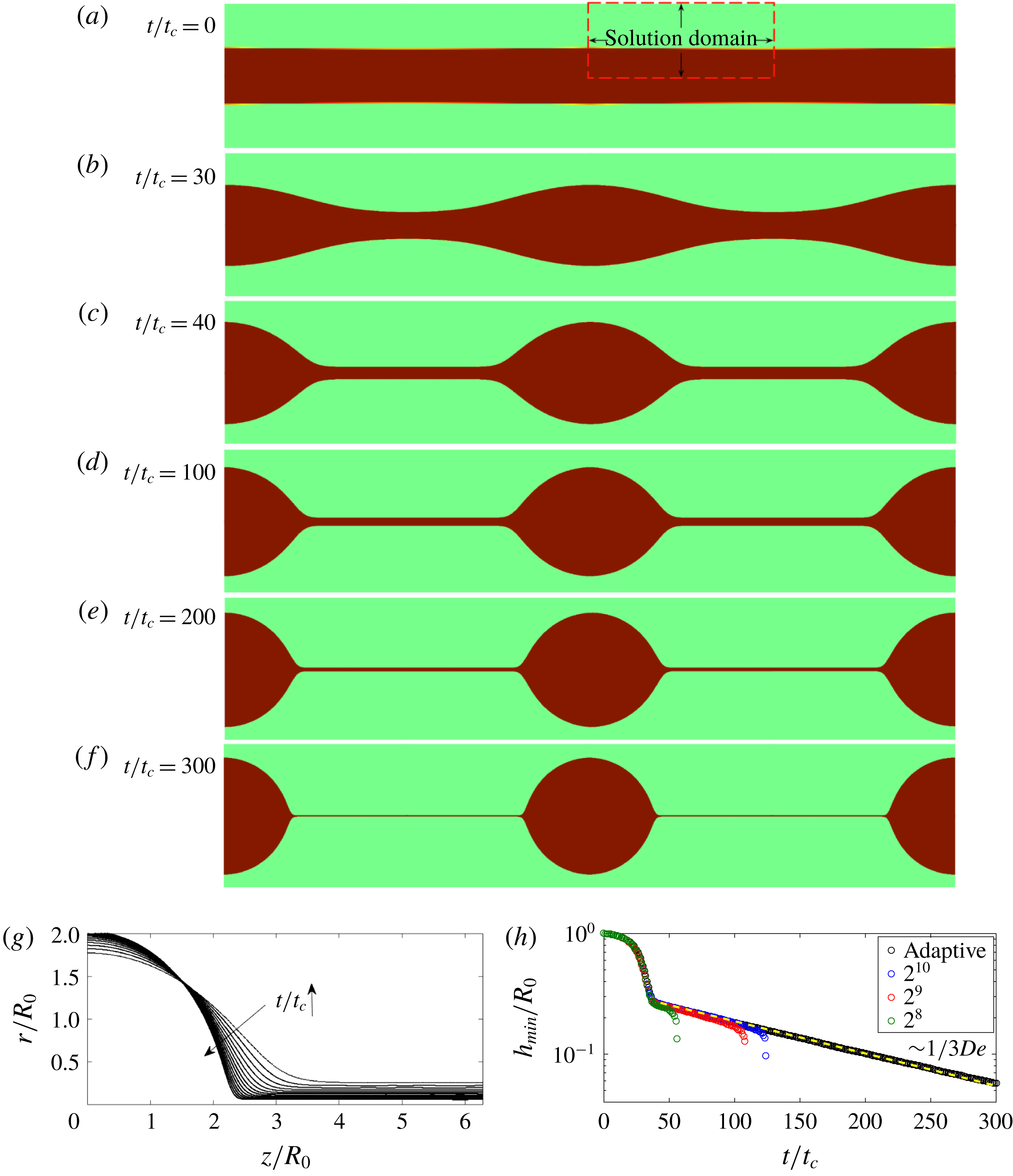
Filament thinning simulation results for Oldroyd-B constitutive equations in an axially symmetric domain. The simulation parameters are similar to those presented in Clasen et al. (Reference Clasen, Eggers, Fontelos, Li and McKinley2006):
 $De=60$
,
 $Oh=3.16$
and
 $\unicode[STIX]{x1D6FD}=0.25$
. (a–e) Snapshots of the thinning of the liquid bridge obtained by adding the interface profiles periodically at (a)
 $t/t_{c}=0$
, (b)
 $t/t_{c}=30$
, (c)
 $t/t_{c}=40$
, (d)
 $t/t_{c}=150$
and (e)
 $t/t_{c}=300$
. The solution domain is axially symmetric and is shown with the red rectangle with dashed edges in (a). Periodicity and symmetry are used to create the images. The bottom boundary is the axially symmetry axis. The left and right wall boundary conditions are symmetry boundary conditions as well. (g) Evolution of the interface between
 $t/t_{c}=50$
and
 $t/t_{c}=300$
. The time difference between each curve is
 $\unicode[STIX]{x0394}t=20t_{c}$
. The neck region connecting the thread with the drop becomes steeper as time proceeds. (h) The minimum radius of the filament as a function of time. Exponential thinning starts after
 $t/t_{c}\approx 40$
. The exponential fit to the polymeric thinning shows good agreement with the theory, which states for
 $h_{min}$
that
 $h_{min}(t)/R_{0}=h_{0}/R_{0}\exp [-t/(3Det_{c})]$
. The exponential fit yields
 $h_{0}/R_{0}=0.30$
for
 $De=60$
with an
 $R$
-square error of 0.9968. Convergence of this thinning is observed as a function of the grid size, allowing the thinning to be solved for longer times.

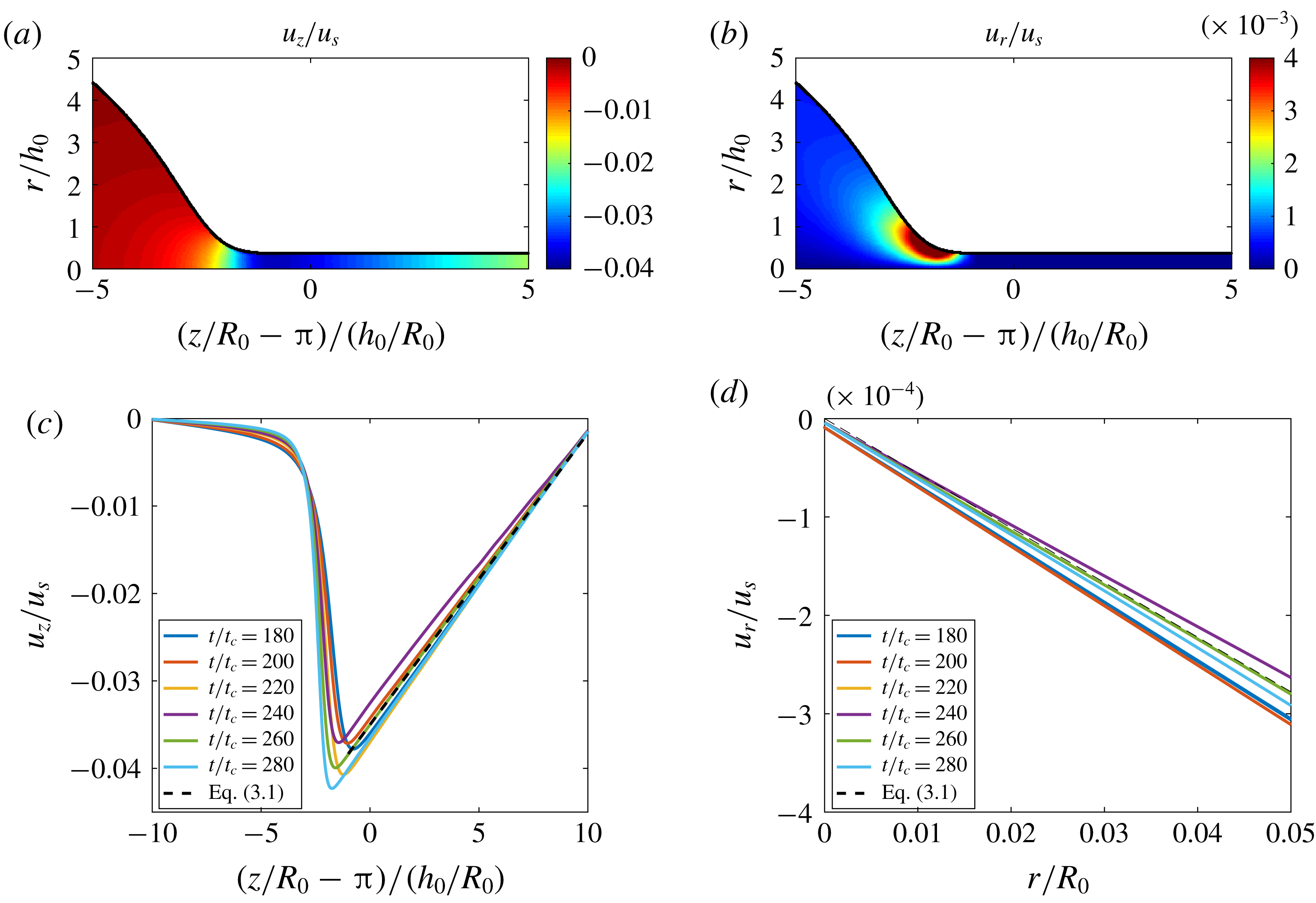
The dimensionless axial and radial velocity components from our simulations, where the length scale is normalized by the filament radius and the time scale is normalized by the capillary time scale,
 $t_{c}=\sqrt{\unicode[STIX]{x1D70C}R_{0}^{3}/\unicode[STIX]{x1D6FE}}$
, so that the velocity scale is
 $u_{s}=R_{0}/t_{c}$
. (a) Colourmap of the axial velocity component,
 $u_{z}/u_{s}$
, at
 $t/t_{c}=180$
as a representative case. An axial flux is directed towards the drop from the thinning thread, and this flux results in the growth of the drop while the connected filament thins. The radial change of axial velocity inside the thread can be neglected, so that
 $\unicode[STIX]{x2202}u_{z}/\unicode[STIX]{x2202}r\approx 0$
. (b) Colourmap of the radial velocity component,
 $u_{r}/u_{s}$
, at
 $t/t_{c}=180$
as a representative case. The radial velocity has a maximum at the interface where the filament is connected to the drop. The axial change of the radial velocity can be neglected inside the thread,
 $\unicode[STIX]{x2202}u_{r}/\unicode[STIX]{x2202}z\approx 0$
. (c) The axial velocity component along
 $r/R_{0}=0$
at different times. The linear part corresponding to the thinning thread has a slope of
 $2\dot{\unicode[STIX]{x1D701}}$
at all times like the plotted theory line. (d) The radial velocity component along
 $z/R_{0}=2\unicode[STIX]{x03C0}$
at different time steps. This component should have a slope of
 $-\dot{\unicode[STIX]{x1D701}}$
at all times like the plotted theory line.

The simulation is started with a liquid cylinder of initial radius
 $R_{0}$
and a perturbation
 $\unicode[STIX]{x1D716}=0.05$
. The non-dimensional parameters are
 $De=60$
,
 $Oh=3.16$
,
 $\unicode[STIX]{x1D6FD}=0.25$
,
 $\unicode[STIX]{x1D70C}_{a}/\unicode[STIX]{x1D70C}_{s}=\unicode[STIX]{x1D702}_{a}/\unicode[STIX]{x1D702}_{s}=0.01$
, which are representative of a high-Deborah-number liquid bridge thinning configuration. Figure 1(a–f) shows the time evolution of the filament, with the initially perturbed liquid bridge starting to thin (a,b), developing a rather slender filament and a drop (c,d). The thinning proceeds exponentially (e,f), with viscoelastic effects allowing for the formation of a very thin film of radius down to 5 % of the initial drop (f). Figure 1(g) shows the time evolution of the interface from
 $t/t_{c}=40$
to
 $t/t_{c}=300$
. The minimum filament radius,
 $h_{min}$
, as a function of time is presented in figure 1(h), showing excellent agreement with the prediction given in (1.2),
 $h_{min}(t)/R_{0}=(h_{0}/R_{0})\exp [-t/(3Det_{c})]$
. When we fit the polymeric thinning from
 $t/t_{c}=40$
to
 $t/t_{c}=300$
, we obtain
 $h_{0}/R_{0}=0.30$
for
 $De=60$
with an
 $R$
-square error of 0.99, in very good agreement with the theory (Clasen et al.
Reference Clasen, Eggers, Fontelos, Li and McKinley2006), where
 $h_{0}/R_{0}=Oh(1-\unicode[STIX]{x1D6FD})/De=0.27$
. These results show that our model can capture the polymeric thinning successfully and follow the theoretical prediction for the thinning. From our numerical experiments, we note that changes of
 $\unicode[STIX]{x1D70C}_{a}/\unicode[STIX]{x1D70C}_{s}$
and
 $\unicode[STIX]{x1D702}_{a}/\unicode[STIX]{x1D702}_{s}$
have no observable effects on our results as long as these ratios are smaller than 0.1. Change of
 $Oh$
only affects the exponential thinning starting time, with larger
 $Oh$
delaying the thinning due to viscous effects. We also note that decrease in
 $\unicode[STIX]{x1D6FD}$
increases the stiffness of the problem, and when
 $\unicode[STIX]{x1D6FD}$
is reduced, the initial part of the thinning becomes faster (due to the smaller solvent viscosity) before the exponential thinning starts.
The independence of the filament thinning on the grid size is shown in figure 1(h). Three fixed grids with
 $2^{8}$
,
 $2^{9}$
and
 $2^{10}$
grid points along one edge of the square domain (of length
 $2\unicode[STIX]{x03C0}$
) are shown to collapse together with the adaptive scheme, which uses functions that refine the grid according to the numerical error in velocity and the curvature in both the axial and radial directions. We see that the adaptive scheme yields the same results at early time steps with the uniform
 $2^{10}$
grid, but a higher refinement is required at later times when the filament thins significantly, because the thinning reaches a width close to the mesh size. The adaptive scheme refines the grid up to
 $2^{12}$
, which allows the simulations to reach later time steps, and we can capture the thinning up to 5.0 % of the initial radius with at least 40 grid points along the thin filament in the radial direction.
Colourmaps of the polymeric stress components at
 $t/t_{c}=180$
as a representative case that shows the typical distribution of stresses. (a) The axial component,
 $\unicode[STIX]{x1D70E}_{zz}/\unicode[STIX]{x1D70E}_{s}$
. (b) The radial component,
 $\unicode[STIX]{x1D70E}_{rr}/\unicode[STIX]{x1D70E}_{s}$
. (c) The off-diagonal component,
 $\unicode[STIX]{x1D70E}_{rz}/\unicode[STIX]{x1D70E}_{s}$
. We observe that the axial stress has the largest magnitude. We also see that
 $\unicode[STIX]{x1D70E}_{rz}$
is actually significant and it cannot be neglected compared with
 $\unicode[STIX]{x1D70E}_{rr}$
, while remaining small compared with
 $\unicode[STIX]{x1D70E}_{zz}$
.

The axial and radial velocity components are important to understand the filament thinning. Figure 2(a) and (b) show the normalized velocity fields
 $u_{z}/u_{s}$
and
 $u_{r}/u_{s}$
respectively as functions of the normalized length scales
 $(z/R_{0}-\unicode[STIX]{x03C0})/(h_{0}/R_{0})$
and
 $(r/R_{0})/(h_{0}/R_{0})$
, with
 $u_{s}=R_{0}/t_{c}$
at
 $t/t_{c}=180$
. Figure 2(a) shows that there is an axial flux directed towards the drop from the filament, which results in growth of the drop while the connected filament thins. This figure also shows that the radial change of axial velocity inside the thread can be neglected, so that
 $\unicode[STIX]{x2202}u_{z}/\unicode[STIX]{x2202}r\approx 0$
. Figure 2(b) shows that the radial velocity is maximum in the neck region where the filament is connected to the drop. Similarly, inside the polymeric thinning region, the axial change of the radial velocity can be neglected,
 $\unicode[STIX]{x2202}u_{r}/\unicode[STIX]{x2202}z\approx 0$
.
The axial velocity along the axial direction (
 $r/R_{0}=0$
) in the filament is presented in figure 2(c), while the radial velocity along the radial direction (
 $z/R_{0}=2\unicode[STIX]{x03C0}$
) in the filament is shown in figure 2(d). As shown by Clasen et al. (Reference Clasen, Eggers, Fontelos, Li and McKinley2006), using the continuity equation, the axial velocity component along the thread is
 $$\begin{eqnarray}u_{z}(r,z,t)/u_{s}=2\dot{\unicode[STIX]{x1D701}}z/R_{0}+u_{z,0},\end{eqnarray}$$
where
 $u_{z,0}=-4\unicode[STIX]{x03C0}\dot{\unicode[STIX]{x1D701}}$
, so the axial velocity at the centre of the filament (
 $z/R_{0}=2\unicode[STIX]{x03C0}$
) connecting two beads is equal to zero. The radial velocity component is
 $$\begin{eqnarray}u_{r}(r,z,t)/u_{s}=-\dot{\unicode[STIX]{x1D701}}r/R_{0},\end{eqnarray}$$
where
 $\dot{\unicode[STIX]{x1D701}}=1/3De$
is the coefficient for the slope. The velocity profiles obtained numerically follow the theoretical predictions given by (3.1) and (3.2) closely, as shown in figures 2(c) and 2(d) respectively.
Now, we examine the polymeric stress components,
 $\unicode[STIX]{x1D70E}_{zz}$
,
 $\unicode[STIX]{x1D70E}_{rr}$
and
 $\unicode[STIX]{x1D70E}_{rz}$
, during the exponential thinning. The one-dimensional slender body approximation does not account for
 $\unicode[STIX]{x1D70E}_{rz}$
in the formulation of the equation of motion (Clasen et al.
Reference Clasen, Eggers, Fontelos, Li and McKinley2006). In addition, the one-dimensional formulation predicts that the dimensionless axial stress will vary as
 $\unicode[STIX]{x1D70E}_{zz}/\unicode[STIX]{x1D70E}_{s}=\unicode[STIX]{x1D70E}_{0}/\unicode[STIX]{x1D70E}_{s}\exp (t/3Det_{c})$
, where
 $\unicode[STIX]{x1D70E}_{s}=\unicode[STIX]{x1D70C}u_{s}^{2}$
is the characteristic stress scale. The stress components at a representative time during the exponential thinning are presented in figure 3, and indicate that
 $\unicode[STIX]{x1D70E}_{rz}$
cannot be neglected compared with
 $\unicode[STIX]{x1D70E}_{rr}$
. This result is significant because the one-dimensional lubrication approximation does not take
 $\unicode[STIX]{x1D70E}_{rz}$
into account due to the formulation of the slender jet equations. We also note that the distributions of
 $\unicode[STIX]{x1D70E}_{rz}$
and
 $\unicode[STIX]{x1D70E}_{rr}$
are very similar, with their maxima in magnitude around the neck region.
The axial stress component,
 $\unicode[STIX]{x1D70E}_{zz}$
, is shown as a function of the rescaled axial direction,
 $(z/R_{0}-\unicode[STIX]{x03C0})/(h_{0}/R_{0})$
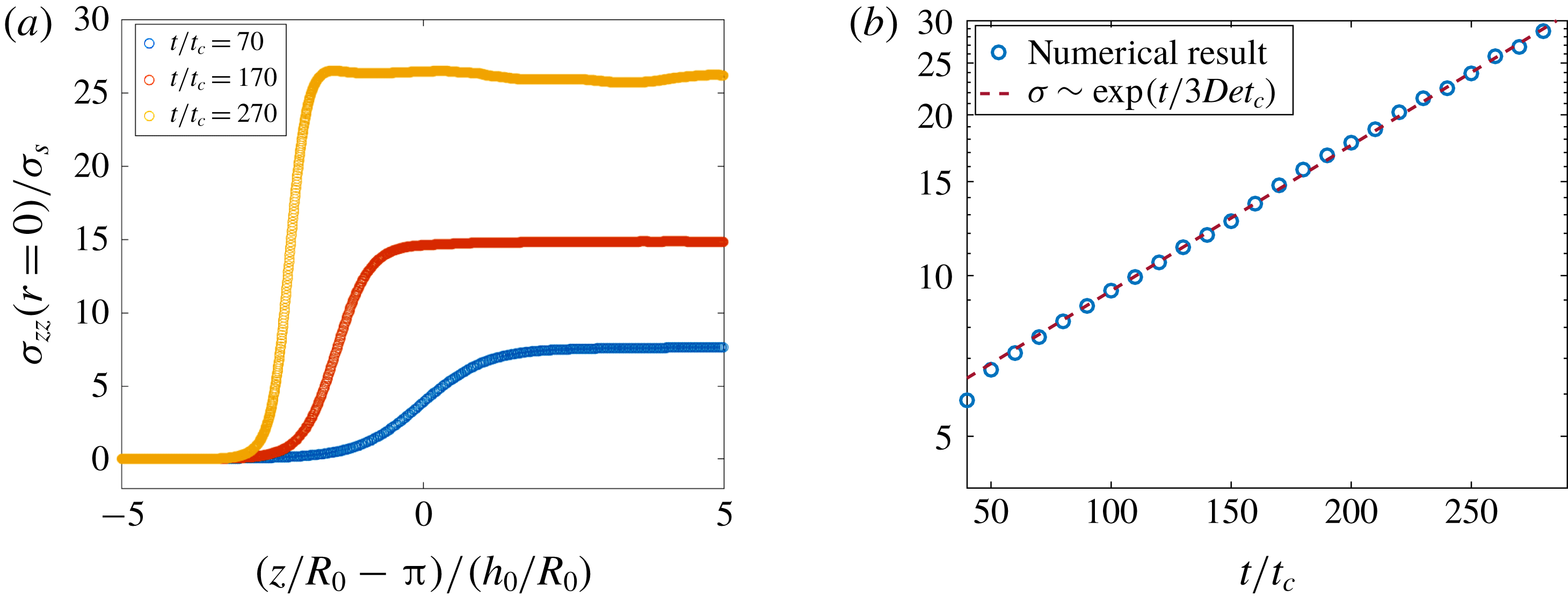
, along
 $r/R_{0}=0$
for different time steps in figure 4(a). We see that the axial stress maintains a flat profile inside the thinning thread over time, while the stress inside the drop is negligible. This means that as the thinning thread supplies the attached drop with more material, a growing stress has to be supported by the thread itself to sustain the integrity of the structure. The change of the axial stress inside the filament as a function of time during the polymeric thinning is shown in figure 4(b) and is found to follow the theoretical prediction, with
 $\unicode[STIX]{x1D70E}_{0}/\unicode[STIX]{x1D70E}_{s}=5.83$
evaluated in the simulation for
 $De=60$
with an
 $R$
-square error of 0.98. This value is close to the predicted
 $\unicode[STIX]{x1D70E}_{0}/\unicode[STIX]{x1D70E}_{s}=2/(h_{0}/R_{0})=6.66$
from the one-dimensional modelling (Clasen et al.
Reference Clasen, Eggers, Fontelos, Li and McKinley2006).
The evolution of the axial stress component,
 $\unicode[STIX]{x1D70E}_{zz}$
, along the filament. (a) A plot of
 $\unicode[STIX]{x1D70E}_{zz}/\unicode[STIX]{x1D70E}_{s}$
as a function of the rescaled axial location,
 $(z/R_{0}-\unicode[STIX]{x03C0})/h_{0}$
, at different times;
 $\unicode[STIX]{x1D70E}_{zz}$
is constant along the filament, as predicted by the slender body approximation; the stress gradient between the drop and the thread becomes larger as the filament thins. (b) A plot of
 $\unicode[STIX]{x1D70E}_{zz}/\unicode[STIX]{x1D70E}_{s}$
at
 $r/R_{0}=0$
as a function of time; the stress increases exponentially with time,
 $\unicode[STIX]{x1D70E}_{zz}(z,t)/\unicode[STIX]{x1D70E}_{s}=\unicode[STIX]{x1D70E}_{0}/\unicode[STIX]{x1D70E}_{s}\exp (t/3Det_{c})$
, with the fitted value
 $\unicode[STIX]{x1D70E}_{0}/\unicode[STIX]{x1D70E}_{s}=5.83$
for
 $De=60$
with an
 $R$
-square error of 0.99.

3.2 Polymeric axial stress profile
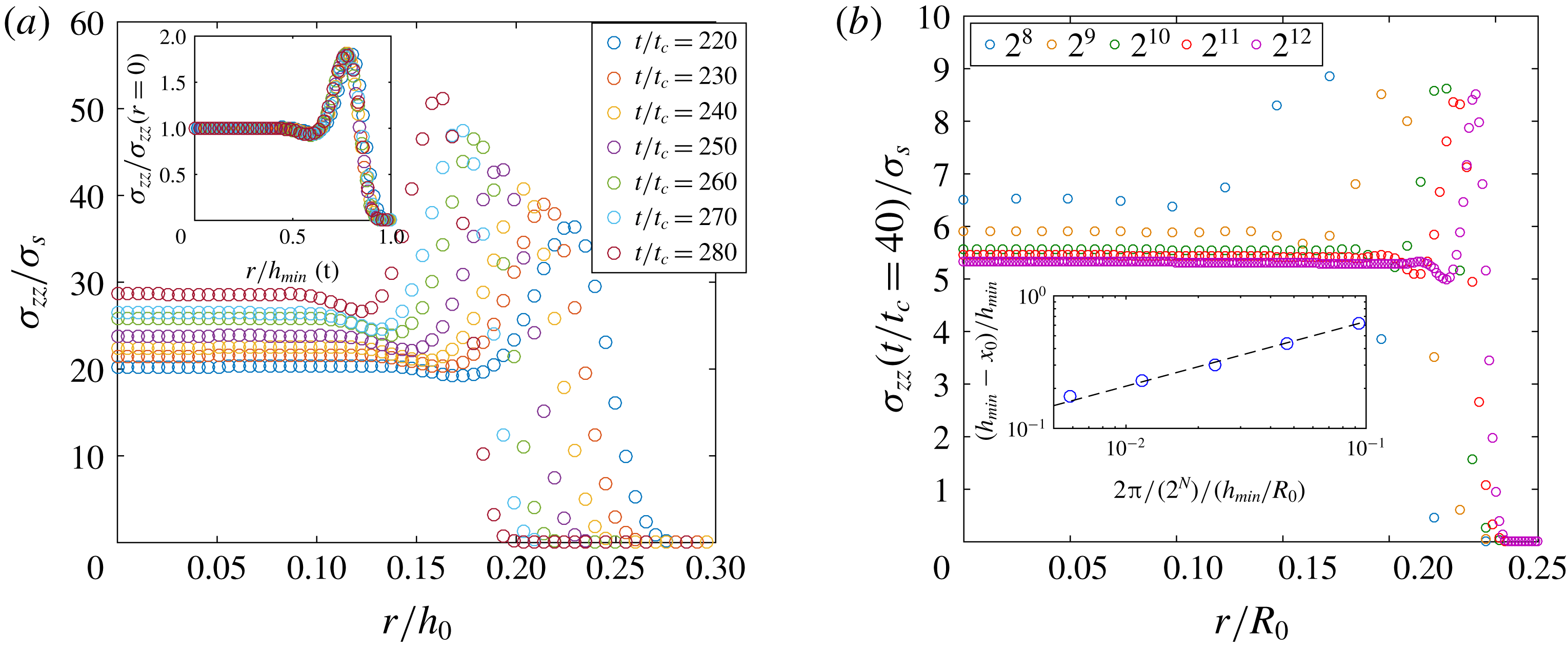
The radial distribution of the polymeric axial stress,
 $\unicode[STIX]{x1D70E}_{zz}$
. (a) A plot of
 $\unicode[STIX]{x1D70E}_{zz}/\unicode[STIX]{x1D70E}_{s}$
as a function of the scaled radial coordinate,
 $r/h_{0}$
, along the filament. The stress goes to zero beyond the interface with the ambient air. The stress profile exhibits similarity, so that all data can be rescaling into a single curve by
 $\unicode[STIX]{x1D70E}_{zz}(r/R_{0}=0)/\unicode[STIX]{x1D70E}_{s}$
and
 $r/h_{min}(t)$
(inset). (b) The grid size dependence of the stress profile (evaluated at
 $t/t_{c}=40$
). As the number of grid points,
 $2^{N}$
, is increased, the peak stress location is pushed towards the interface and the size of the bump gets smaller. The inset shows that the normalized bump size,
 $(h_{min}-x_{0})/h_{min}$
, decreases as the grid size increases,
 $(2\unicode[STIX]{x03C0}/2^{N})/(h_{min}/R_{0})$
, where
 $x_{0}$
denotes the distance where the stress starts to deviate from the uniform value measured from the centre,
 $r=0$
. The dashed line is a power-law fit,
 $1.97x^{-0.50}$
.

Figure 5(a) shows the distribution of
 $\unicode[STIX]{x1D70E}_{zz}$
as a function of the rescaled radial direction,
 $r/h_{0}$
, at different times, and we observe a peculiar profile. As the time proceeds, the peak stress and the stress at
 $r=0$
increase exponentially, and the peak stress location shifts towards the symmetry axis as the filament thins. We show in the inset of figure 5(a), by rescaling the axial stress component along the interface with the stress at
 $r=0$
,
 $\unicode[STIX]{x1D70E}_{zz,r=0}$
, and the radial coordinate with the interface thickness at that time,
 $r/h_{min}(t)$
, so that
 $r/h_{min}=1$
denotes the interface, that the radial distribution of the stress is similar in time where the ratio of the peak stress to the stress at the centre of the filament is preserved along with the size of the stress bump. We note that this profile is similar to the ‘boundary layer stress profile’ in stretching viscoelastic filament simulations presented in the literature (Yao & McKinley Reference Yao and McKinley1998).
The radial distribution of the polymeric axial stress depicted in figure 5(a) is unexpected. We investigate the width of the non-uniform region and the magnitude of the peak stress change with the grid size. Figure 5(b) shows the results at the time step
 $t/t_{c}=40$
for increasing grid size, with
 $2^{N}$
the number of grid points along the filament in the axial direction (
 $N$
from 8 to 12). The time
 $t/t_{c}=40$
is chosen because it is after the polymeric thinning starts and before the
 $2^{8}$
grid filament breaks up. The width of the non-uniform stress region decreases with increasing refinement and the peak stress location is pushed towards the filament–air interface. The normalized non-uniform stress bump width,
 $(h_{min}-x_{0})/h_{min}$
, as a function of the grid size,
 $2\unicode[STIX]{x03C0}/(2^{N})/h_{min}$
, at time
 $t/t_{c}=40$
is shown in figure 5(d), where
 $x_{0}$
is the distance where the stress starts to deviate from the uniform value measured from the centre,
 $r=0$
. We see that the width of the non-uniform stress region as a function of the normalized grid size decreases according to a power-law relationship, with a coefficient of
 $-0.5$
. As the grid size increases, the bump width gets smaller with an unchanged peak stress value, suggesting that the bump would become infinitely thin as the resolution keeps increasing, with a peak value that does not depend on the resolution. While this grid-dependent polymeric axial stress structure, which might be a numerical artefact, is observed, it does not have an apparent effect on the evolution of the minimum filament thinning and velocity components, which are in excellent agreement with the predictions presented in (1.2) and (1.3).
3.3 Self-similar profile and comparison with experiments
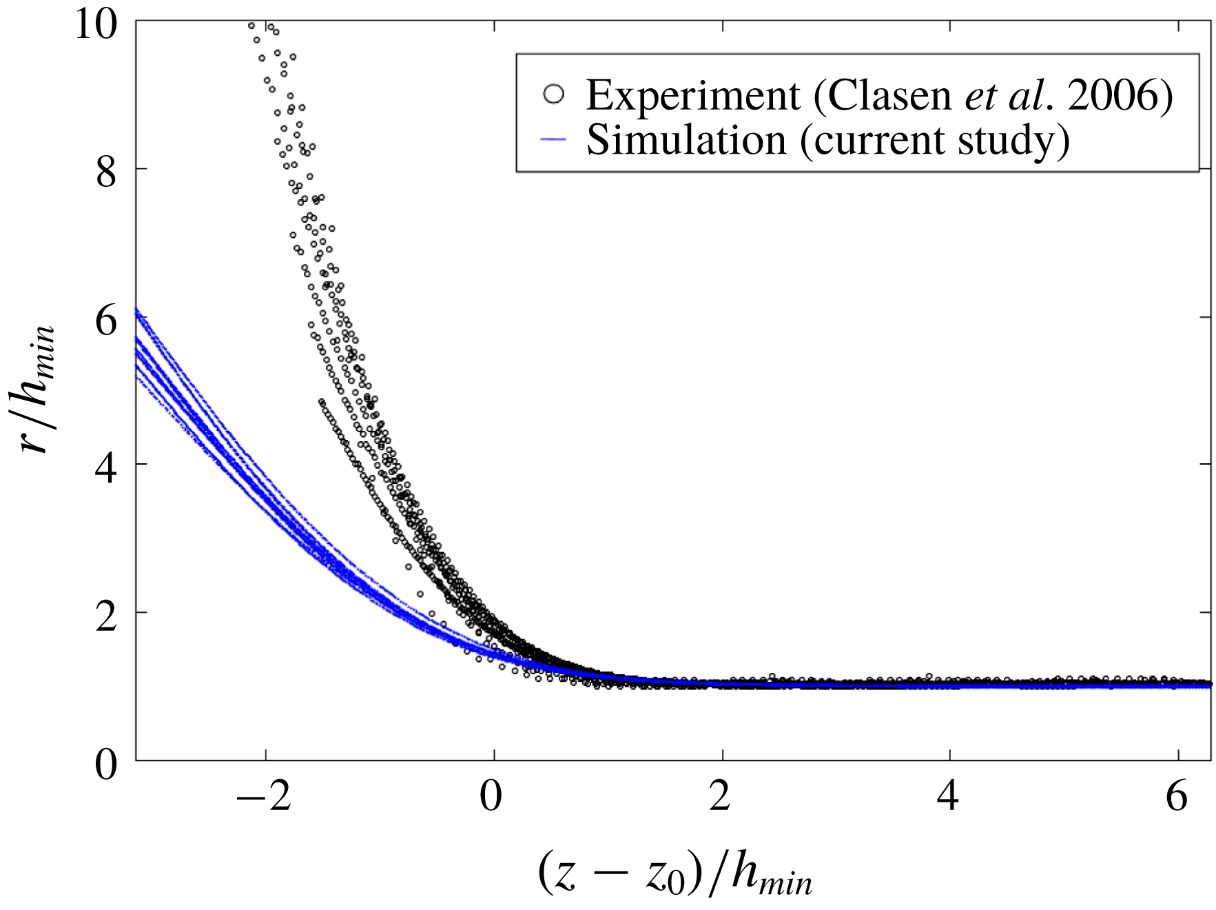
We compare our numerical results for the interface profiles with the experimental data presented by Clasen et al. (Reference Clasen, Eggers, Fontelos, Li and McKinley2006) in figure 6, showing
 $r/h_{min}$
as a function of
 $(z-z_{0})/h_{min}$
for the final stages of the thinning. The numerical profiles are plotted for
 $10t/t_{c}$
intervals from
 $t/t_{c}=220$
to
 $t/t_{c}=300$
, with
 $z_{0}$
the numerically determined axial location of the maximum radial velocity. We observe that while both the numerical and experimental profiles present clear self-similar dynamics, the slopes of the experimental profiles turn out to be steeper than the slopes of the numerical results, as discussed for the one-dimensional modelling (Clasen et al.
Reference Clasen, Eggers, Fontelos, Li and McKinley2006).
The self-similar thinning obtained from the present simulation and the experimental data from Clasen et al. (Reference Clasen, Eggers, Fontelos, Li and McKinley2006) for a liquid bridge with
 $R_{0}=3~\text{mm}$
,
 $\unicode[STIX]{x1D6FE}=37~\text{mN}~\text{m}^{-1}$
,
 $\unicode[STIX]{x1D70C}=1026~\text{kg}~\text{m}^{-3}$
, solvent viscosity
 $\unicode[STIX]{x1D702}_{s}=65.2~\text{Pa}~\text{s}$
, polymeric viscosity
 $\unicode[STIX]{x1D702}_{p}=9.8~\text{Pa}~\text{s}$
and relaxation time
 $\unicode[STIX]{x1D706}=8.1~\text{s}$
. The last nine experimental profiles taken in intervals of 0.5 s are shown, and rescaled by
 $h_{min}$
measured experimentally. The numerical results are for
 $10t/t_{c}$
time steps from
 $t/t_{c}=220$
to
 $t/t_{c}=300$
, with
 $z_{0}$
the location where the radial velocity component is maximum and
 $h_{min}$
determined numerically. Both the numerical and the experimental data present a self-similar evolution with time, but the experimental data are much sharper.

3.4 Simulating the beads-on-a-string structure
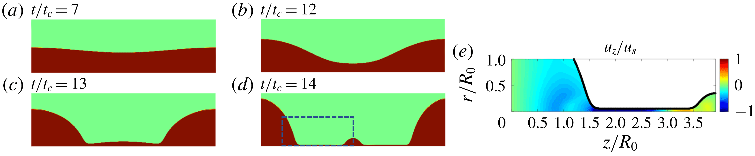
The beads-on-a-string structure simulated with the two-dimensional model in an axially symmetric domain. (a–d) Snapshots of the thinning liquid bridge that results in the satellite drop formation at (a)
 $t/t_{c}=7$
, (b)
 $t/t_{c}=12$
, (c)
 $t/t_{c}=13$
and (d)
 $t/t_{c}=14$
. (e) Colourmap of the axial velocity component,
 $u_{z}/u_{s}$
, at
 $t/t_{c}=14$
, within the area shown by the dashed line in (d). Inside the filament, there are fluxes towards both the large and the small drops.

Our numerical model can be used for the canonical beads-on-a-string structure, as an example for possible applications. We consider parameters within the range of existence of beads-on-a-string (Wagner et al.
Reference Wagner, Amarouchene, Bonn and Eggers2005), and studied using a one-dimensional model with parameters by Ardekani et al. (Reference Ardekani, Sharma and McKinley2010),
 $Oh=0.04$
,
 $De=0.8$
,
 $\unicode[STIX]{x1D6FD}=0.27$
, and an initial sinusoidal perturbation
 $\unicode[STIX]{x1D716}=0.05$
. We obtain the expected beads-on-a-string structure with two large drops connected with a satellite droplet, as shown in figure 7(a–d). The aspect ratio of the satellite to the large droplet is found to be similar to previous one-dimensional work (Ardekani et al.
Reference Ardekani, Sharma and McKinley2010). We also show the distribution of the axial velocity,
 $u_{z}/u_{s}$
, in figure 7(e). It is seen that the filament thins while the fluxes are directed towards both the satellite and the main drops.
4 Conclusions
We present direct numerical simulations of the two-phase axisymmetric momentum equations for viscoelastic thinning of an Oldroyd-B fluid, and employ the log-conformation technique to overcome the high-Weissenberg-number problem. The thinning of the filament and its velocity as a function of time are successfully modelled and can be described by the one-dimensional theory derived from slender body approximations. The polymeric stress components of the thinning filament are examined, and the off-diagonal stress component,
 $\unicode[STIX]{x1D70E}_{rz}$
, is not negligible, while it is not taken into account by one-dimensional formulations. Furthermore, the axial stress component,
 $\unicode[STIX]{x1D70E}_{zz}$
, exhibits a self-similar radial distribution in time. This structure exhibits grid-dependent properties while not having an apparent effect on the outcome of the simulation results in terms of the velocity and filament thinning. It should be noted that, using the Oldroyd-B model, we did not capture the blistering instability observed experimentally on stretched viscoelastic filaments (Chang, Demekhin & Kalaidin Reference Chang, Demekhin and Kalaidin1999; Sattler, Wagner & Eggers Reference Sattler, Wagner and Eggers2008), which may require the implementation of an extension of the Oldroyd-B model (Eggers Reference Eggers2014) to solve for the polymer and solvent phases inside the filament separately. With this study, we demonstrate the ability to perform simulations of complex two-dimensional viscoelastic flows, which opens the way for the development of viscoelastic models for real-life applications.
Acknowledgements
We are grateful to S. Popinet and W. Mostert for discussions about viscoelastic simulations using Basilisk. The computations were partially performed using allocation TGOCE140023 to L.D. from the Extreme Science and Engineering Discovery Environment (XSEDE), supported by NSF grant no. ACI-1053575. J.E. acknowledges support from the Leverhulme Trust through International Academic Fellowship IAF-2017-010. This work is also supported by the National Science Foundation (NSF) through a Materials Research Science and Engineering Center (MRSEC) program (DMR-1420541).