





1. Introduction
It has been known since the 1950s that supersonic flows over axisymmetric spiked blunt bodies in a uniform free stream can exhibit violent pulsating unsteadiness. One way to think of such bodies is as double cones, with the first-cone angle,  $\theta _1$, being small and the second,
 $\theta _2\leq {\rm \pi}/2$, large. Of course, in the case when
 $\theta _1 = \theta _2$, this is the axisymmetric flow over a (finite) cone, which is known to be steady. Therefore, in the
 $\theta _1$–
 $\theta _2$ space, there must exist a boundary that separates the region of steady from that of unsteady flow. The aim of this work is to determine this boundary. Obviously, there are other geometric and physical dimensionless variables that are pertinent to this problem and these will be discussed later.
It is useful to aid the discussion with two sketches that illustrate two manifestations of steady flows over double cones, see figure 1. A first cone of angle  $\theta _1$, small enough for the cone 1 shock to be attached and of length
 $\ell _1$ is followed by a second cone of angle
 $\theta _2$ and length
 $\ell _2$. The cone 2 shock causes the boundary layer developing on cone 1 to separate. The separation deflects the flow again and causes the separation shock. In (a) the separation length is relatively long, so that reattachment occurs on cone 2, where a reattachment shock ensues. If
 $\theta _2$ is sufficiently large, the cone 2 shock is detached and curved with a subsonic flow region downstream of it. This is the situation shown in the sketch. The interaction of the reattachment shock with the other shocks initiates a supersonic shock train, which may or may not penetrate through to the shoulder of cone 2. In (b), the separation length is quite small and reattachment occurs on cone 1. Again a supersonic shock train occurs. These sketches also define the three dimensionless geometrical parameters of the problem
 \begin{equation} \theta_1, \theta_2\quad \textrm{and} \quad\varLambda=\ell_2/\ell_1. \end{equation}
Schematic sketches of two forms of steady double-cone flow. (a) The reattachment occurs on cone 2. (b) The separation bubble is small and reattachment occurs almost immediately on cone 1. In both cases only the beginning of a supersonic shock train is indicated following the reattachment. This may or may not reach and penetrate the sonic surface, indicated by a dashed line.

Unsteady double-cone flows have been studied extensively in the case when  $\theta _1$ is near zero, i.e. spiked-body flow. Detailed reviews have been presented by Kenworthy (Reference Kenworthy1978) and Ahmed & Qin (Reference Ahmed and Qin2011), and we restrict discussion to a few contributions that are relevant to our aim. Mair (Reference Mair1952) investigated supersonic flow at Mach number 1.96 over blunt bodies with a forward pointing spike experimentally and was the first to observe the pulsating unsteadiness. Shortly thereafter, Stollery, Maull & Belcher (Reference Stollery, Maull and Belcher1960) had taken a hypersonic gun tunnel into operation at Imperial College, London. In two early projects studied in this facility, Maull (Reference Maull1960) and Wood (Reference Wood1961) confirmed the unsteady behaviour in the hypersonic range for spiked blunt bodies and spiked cones, respectively. Wood (Reference Wood1961) recognized the importance of the detachment angle of cone 2,
 $\theta _{2d}$, in the unsteadiness boundary and presented a map in
 $\theta _2$–
 $\varLambda$ space in which boundaries between different flow types were drawn. He distinguished between pulsating unsteadiness at larger
 $\theta _2$ and a milder oscillating flow at smaller
 $\theta _2$. The promise of using a spike, that it might cause drag and heat-load reduction, which also motivated an investigation by Bogdonoff & Vas (Reference Bogdonoff and Vas1959), was thus disappointed.
Spiked cones were also part of the high Mach number investigation by Holden (Reference Holden1966) extending the map of Wood (Reference Wood1961) and including detailed heat-load measurements. A very detailed and wide-ranging experimental investigation of spiked cone flow was performed by Kenworthy (Reference Kenworthy1978), who further extended Wood's map and analysed and classified pressure traces and Strouhal numbers of the unsteady flows. It is interesting that Kenworthy's data indicate that the unsteadiness boundary in  $\theta _2$–
 $\varLambda$ space is virtually independent of
 $\varLambda$ for
 $\varLambda \geq 0.5$ and lies approximately at
 $\theta _2=\theta _{2d}$. This differs from the Wood (Reference Wood1961) and Holden (Reference Holden1966) maps which show the boundary at
 ${\sim }15^\circ$ above
 $\theta _{2d}$ for
 $M=10$ at
 $\varLambda =0.5$. Kenworthy found that the pulsating unsteadiness was insensitive to Reynolds number.
A thorough computational investigation of one of Kenworthy's cases was presented by Feszty, Badcock & Richards (Reference Feszty, Badcock and Richards2004), which reproduced the features of the experiment in great detail. A computational study of the more general spiked blunt body flow was presented by Panaras & Drikakis (Reference Panaras and Drikakis2009).
The work on unsteadiness was mainly restricted to the case when  $\theta _1$ is effectively zero, i.e. to spiked bodies. Where it concerned spiked cones, the emphasis was on resolving the
 $\theta _2$–
 $\varLambda$ space at zero
 $\theta _1$. Two main types of unsteadiness were observed as
 $\varLambda$ was increased. At small
 $\varLambda$ the flow is steady. Then with
 $\varLambda$ increasing, a transition to the ‘oscillatory’ flow was followed by a transition to the ‘pulsating’ flow, the main distinction between them being amplitude. Several authors also observed hysteretic behaviour related to the direction of
 $\varLambda$ change. With the exception of a single case found by Kenworthy (Reference Kenworthy1978) no unsteadiness was observed for
 $\theta _2<\theta _{2d}$. This case was the oscillatory type at
 $\theta _2 \sim 5^\circ$ below the detachment angle.
In the case of finite  $\theta _1$, the emphasis has been on steady flows, a dominating purpose being testing of computations. The separation length and the distributions of skin friction and heat flux are particularly sensitive features of such flows and difficult to reproduce computationally. An extensive investigation representative of this area is that by Holden et al. (Reference Holden, Wadhams, Harvey and Candler2007), which includes detailed experimental data on double-cone flows with
 $\theta _1=25^\circ$ and
 $\theta _2=55^\circ$. This provided test cases for various kinds of numerical simulations. The sensitivity of this configuration to non-equilibrium high-enthalpy real-gas phenomena was used by Olejniczak, Candler & Hornung (Reference Olejniczak, Candler and Hornung1997) to test computational models against free-piston shock tunnel experiments. Three models with
 $\theta _1=25^\circ$ and
 $\theta _2=65^\circ$, 68
 $^\circ$ and 70
 $^\circ$ were tested in high-enthalpy nitrogen flow, and holographic interferograms were taken. At the two larger values of
 $\theta _2$ evidence of unsteadiness was found. More such free-piston shock tunnel results including high-speed video visualizations were presented by Knisely (Reference Knisely2016) for (
 $\theta _1, \theta _2$) = (25
 $^\circ$, 55
 $^\circ$). While the main shocks in these were steady during the run, the shear layer at the edge of the supersonic shock train was unsteady.
A case in which the stability and conditional unsteadiness of double-cone flows other than that with  $\theta _1=0$ was studied was Tumuklu, Theofilis & Levin (Reference Tumuklu, Theofilis and Levin2018), in which the area around the separation region and the supersonic shock train was analysed theoretically and computationally. In that case the stability was clearly Reynolds-number dependent.
In summary, previous work on the unsteadiness boundary in double-cone flows has centred on exploring the  $\theta _2$–
 $\varLambda$ space at
 $\theta _1=0$. Instead, in the present work, the aim is to search for the boundary in the
 $\theta _1$–
 $\theta _2$ space with only two values of
 $\varLambda$: 0.5 and 1. Knowledge of this boundary would be valuable, e.g. in the design of experiments that test computational models.
2. Parameters
This investigation is restricted to nitrogen flows with a constant ratio of specific heats  $\gamma =1.4$ and, in one case, thermally perfect carbon dioxide. Any dimensionless quantity
 $Q$, which may here be thought of as a function describing the unsteadiness boundary, will therefore be
 \begin{equation} Q=Q(\theta_1,\theta_2,\varLambda,M_\infty,\gamma,Re,T_w/T_0), \end{equation}
where  $M_\infty$ is the free-stream Mach number,
 $Re=\rho _\infty U_\infty \ell _1/\mu _\infty$ is the Reynolds number with free-stream density, velocity and viscosity and
 $T_w/T_0$ is the wall to total temperature ratio.
In the hypersonic Mach number range, the separate dependence on Mach number and  $\gamma$ may be lumped into dependence on a single parameter, the inverse normal-shock density ratio
 \begin{equation} \varepsilon=\frac{\gamma-1+2/M_\infty^2}{\gamma+1}. \end{equation}
For example, the detachment angle of a cone is very well approximated, see Hayes & Probstein (Reference Hayes and Probstein1959), by
 \begin{equation} \theta_d=2 \arctan\sqrt{\frac{2}{\varepsilon}}-\frac{\rm \pi}{2}. \end{equation}
In all but one of the cases considered ( $M_\infty =2$) this lumping together of
 $M_\infty$ and
 $\gamma$ is justified, and even for
 $M_\infty$ as low as 2, for which
 $\varepsilon =0.375$, the error made by the approximation for
 $\theta _d$ is only 43
 $^\circ$ vs the true value 41.5
 $^\circ$. At
 $M_\infty =4$, with
 $\gamma =1.4$, this difference reduces to 0.6
 $^\circ$ (53.4
 $^\circ$, 52.8
 $^\circ$) and at
 $M_\infty =7.7$ to 0.2
 $^\circ$ (56.6
 $^\circ$, 56.4
 $^\circ$). Also, in all cases except
 $M_\infty =2$, the wall to total temperature ratio is small. Thus, for hypersonic flow, the problem is reduced to five independent parameters
 \begin{equation} Q=Q(\theta_1,\theta_2,\varLambda,\varepsilon,Re). \end{equation}
It is clear that the unsteadiness boundary is strongly influenced by the cone 2 detachment angle,  $\theta _{2d}$. It is therefore desirable that a large range of
 $\theta _{2d}$ values be considered. For this reason one of the cases in the study is that of thermally perfect carbon dioxide. The four vibrational degrees of freedom of CO
 $_2$ cause the specific heats to be quite large when they are excited, and, at the condition considered for that case,
 $\varepsilon =0.091$ so that
 $\theta _{2d}=65.9^\circ$. This value of
 $\varepsilon$ was determined by measuring the density ratio across the normal part of the cone 2 shock in one of the CO
 $_2$ computations. A summary of the conditions considered is given in table 1.
Free-stream conditions of the cases computed.

Condition A’ differs from A only in the doubling of the value of  $p_{\infty }$ in order to get an idea of the effect of
 $Re$. While it is clear from the range of parameters that some of these flows will exhibit temperatures that are high enough for nitrogen to be at least vibrationally excited in physical flows, these degrees of freedom are deliberately kept unexcited and the gas is constrained to be perfect with constant
 $\gamma =1.4$. This is not true in the carbon dioxide case, where vibrational equilibrium is assumed.
3. Computational matters
3.1. The software
The Eilmer flow simulation software is a derivative of the Navier–Stokes solver described by Jacobs (Reference Jacobs1991). It has been further developed over the years, especially for high-temperature hypersonic flows, and with some significant effort toward verification by Gollan & Jacobs (Reference Gollan and Jacobs2013). While the scope of the Eilmer code exceeds its use in this work, the description in this section is limited to the formulation of the code's features that were used in the present simulations.
Eilmer is formulated around the integral form of the conservation equations, which can be written as
 \begin{equation} \frac{\partial}{\partial t} \int_{V} U \,\textrm{d} V ={-} \oint_{S} \left ( \bar{F}_{c} - \bar{F}_{v} \right ) \cdot \hat{n}\,\textrm{d} A + \int_{V} Q \,\textrm{d} V, \end{equation}
where  $S$ is the bounding surface and
 $\hat {n}$ is the outward-facing unit normal of the control surface. For axisymmetric flow, the symbol
 $V$ in (3.1) is the volume and
 $A$ the area of the cell boundary per radian in the circumferential direction. For a single chemical species, the array of conserved quantities is
 \begin{equation} U = \left[\begin{array}{@{}c@{}} \rho \\ \rho v_{x} \\ \rho v_{y} \\ \rho E \end{array}\right], \end{equation}
where the conserved quantities are respectively density,  $x$-momentum per volume,
 $y$-momentum per volume and total energy per volume.
The flux vectors are divided into convective and viscous-transport contributions. With the specific internal energy of the gas being  $u$ and the total specific energy being
 $E = u + \frac {1}{2} v^2$, the convective component is
 \begin{equation} \bar{F}_{c} = \left [ \begin{array}{@{}c@{}} \rho v_{x} \\ \rho v_{x}^{2} + p \\ \rho v_{y} v_{x} \\ \rho E v_{x} + p v_{x} \end{array} \right ] \hat{i} + \left [ \begin{array}{@{}c@{}} \rho v_{y} \\ \rho v_{x} v_{y} \\ \rho v_{y}^{2} + p \\ \rho E v_{y} + p v_{y} \\ \end{array}\right ] \hat{j}, \end{equation}
and the viscous component is
 \begin{equation} \bar{F}_{v} = \left[\begin{array}{@{}c@{}} 0 \\ \tau_{xx} \\ \tau_{yx} \\ \tau_{xx} v_{x} + \tau_{yx} v_{y} + q_{x} \end{array}\right] \hat{i} + \left [ \begin{array}{@{}c@{}} 0 \\ \tau_{xy} \\ \tau_{yy} \\ \tau_{xy} v_{x} + \tau_{yy} v_{y} + q_{y} \end{array}\right] \hat{j}, \end{equation}
where the viscous stresses are
 \begin{equation} \left.\begin{gathered} \tau_{xx} = 2 \mu \frac{\partial v_{x} }{\partial x} + \lambda \left ( \frac{\partial v_{x}}{\partial x} + \frac{\partial v_{y}}{\partial y} + \frac{v_{y}}{y} \right ), \\ \tau_{yy} = 2 \mu \frac{\partial v_{y} }{\partial y} + \lambda \left ( \frac{\partial v_{x}}{\partial x} + \frac{\partial v_{y}}{\partial y} + \frac{v_{y}}{y} \right ), \\ \tau_{xy} = \tau_{yx} = \mu \left ( \frac{\partial v_{x}}{\partial y} + \frac{\partial v_{y}}{\partial x} \right ). \end{gathered}\right\} \end{equation}
Note that the  $x$-coordinate is along the axis of symmetry and
 $y$ is the radial coordinate.
The secondary viscosity coefficient  $\lambda$ is expressed in terms of the primary coefficient
 $\mu$ via Stokes’ hypothesis,
 $\lambda = - \frac {2}{3} \mu$. The components of the viscous heat flux are related to the gradients of temperature as
 \begin{equation} q_{x} = k \frac{\partial T}{\partial x},\quad q_{y} = k \frac{\partial T}{\partial y}.\end{equation}
The vector of source terms in an axisymmetric flow accounts for a contribution to the radial momentum from the pressure and shear stress acting on the out-of-plane faces of the control volume
 \begin{equation} Q = \left [ \begin{array}{c} 0 \\ 0 \\ \left ( p - \tau_{\theta \theta} \right ) A_{xy} / V \\ 0 \end{array} \right], \end{equation}
where  $A_{xy}$ is the projected area of the cell in the (
 $x,y$)-plane and
 \begin{equation} \tau_{\theta\theta} = 2 \mu \frac{v_{y}}{y} + \lambda \left(\frac{\partial v_{x} }{\partial x} + \frac{\partial v_{y} }{\partial y} + \frac{v_{y}}{y}\right). \end{equation}
See Jacobs (Reference Jacobs1991) for a derivation of these terms.
To complete the conservation equations, a thermal model of the gas is used and the transport coefficients are required. For the simulations with nitrogen, an ideal-gas thermal model is assumed with molecular weight  $M_{N2} = 28.0134$ and ratio of specific heats
 $\gamma = 1.4$. The molecular transport coefficients are provided via Sutherland's approximation
 \begin{equation} \mu(T) = \mu_{ref} \frac{T_{ref} + S}{T + S} \left( \frac{T}{T_{ref}} \right)^{3/2}, \end{equation}
with  $\mu _{ref} = 1.663 \times 10^{-5}\ \textrm {Pa}\ \textrm {s}$,
 $T_{ref} = 273 \ \text {K}$ and
 $S = 107\ \text {K}$. The approximation for thermal conductivity is similar, with
 $k_{ref} = 0.0242\ \text {W}\ \text {m}\ \textrm {K}^{-1}$,
 $T_{ref} = 273\ \text {K}$ and
 $S = 150\ \text {K}$.
For the simulations with carbon dioxide, the thermal model and transport coefficients from the NASA chemical equilibrium analysis CEA code (Gordon & McBride Reference Gordon and McBride1994) was used, together with coefficients taken directly from their database.
The conservation equations are applied to each finite-volume cell for which the boundary, projected onto the ( $x,y$)-plane, consists of four straight lines (or cell interfaces). Flux values are estimated at midpoints of the cell interfaces and the integral conservation equation (3.1) is approximated as the algebraic expression
 \begin{equation} \frac{\textrm{d} U}{\textrm{d} t} ={-} \frac{1}{V} \sum_{cell\text{-}surface} \left( \bar{F}_{c} - \bar{F}_{v} \right ) \cdot \hat{n} \,\textrm{d} A + Q, \end{equation}
where  $U$ and
 $Q$ now represent cell-average values.
The full flow domain is subdivided into blocks of finite-volume cells, arranged into two-dimensional structured grids. During a simulation, a halo of ghost cells around each block of cells facilitates the exchange of data between adjacent blocks and the application of boundary conditions. The exchange of data for adjacent blocks is a simple copy of the cell data, prior to the evaluation of the fluxes of conserved quantities across the cell interfaces. Solid-wall boundary conditions are approximated by reflecting the data for cells that are interior to the block, into the corresponding ghost cells. For the convective fluxes, components of velocity in the ghost cells are adjusted to be mirror images of the interior velocities. For no-slip solid-wall boundaries, the velocity at the boundary face is set to zero and temperature is set to a specific value. At the supersonic inflow boundary, constant flow data are copied into the ghost cells while, at the simple outflow boundary, interior-cell flow data are copied into the downstream ghost cells.
Calculation of the fluxes at each cell interface is preceded by an interpolation phase where cell-average quantities are reconstructed index direction by index direction. Having flow data available in the ghost cells allows all interfaces, including those on a boundary, to be treated by the flux calculator as internal interfaces. For each flow variable,  $w$, left and right values (
 $w_L$ and
 $w_R$ respectively) at a cell interface are evaluated as the corresponding cell average value plus a limited higher-order interpolated increment. Given an array of cell centres
 $[L1,L0,R0,R1]$ with the interface of interest located between
 $L0$ and
 $R0$, we fit separate quadratic interpolants to subranges
 $[L1,L0,R0]$ and
 $[L0,R0,R1]$ and then evaluate
 $w_L$ and
 $w_R$ as
 \begin{equation} \left.\begin{gathered} w_L = w_{L0} + \alpha_{L0} \left[ \varDelta_{L+} \times \left( 2 h_{L0} + h_{L1} \right) + \varDelta_{L-} \times h_{R0} \right] s_L, \\ w_R = w_{R0} - \alpha_{R0} \left[ \varDelta_{R+} \times h_{L0} + \varDelta_{R-} \times \left( 2 h_{R0} + h_{R1} \right) \right] s_R, \\ \varDelta_{L-} = \frac{w_{L0} - w_{L1}}{\dfrac{1}{2} \left( h_{L0} + h_{L1}\right)}, \\ \varDelta_{L+} = \frac{w_{R0} - w_{L0}}{\dfrac{1}{2} \left( h_{R0} + h_{L0} \right)} = \varDelta_{R-},\\ \varDelta_{R+} = \frac{w_{R1} - w_{R0}}{\dfrac{1}{2} \left( h_{R0} + h_{R1} \right)}, \\ \alpha_{L0} = \frac{h_{L0} / 2}{h_{L1} + 2 h_{L0} + h_{R0}}, \\ \alpha_{R0} = \frac{h_{R0} / 2}{h_{L0} + 2 h_{R0} + h_{R1}}, \end{gathered}\right\} \end{equation}
where  $h$ represents the width of a cell. The high-order increment is limited by
 $s_L$ and
 $s_R$ and, as described by van Albada, van Leer & Roberts (Reference van Albada, van Leer and Roberts1981), these limiter values are evaluated as
 \begin{equation} \left.\begin{gathered} s_L = \frac{\varDelta_{L-} \varDelta_{L+} + |\varDelta_{L-} \varDelta_{L+}| + \epsilon} {\varDelta_{L-}^2 + \varDelta_{L+}^2 + \epsilon}, \\ s_R = \frac{\varDelta_{R-} \varDelta_{R+} + |\varDelta_{R-} \varDelta_{R+}| + \epsilon} {\varDelta_{R-}^2 + \varDelta_{R+}^2 + \epsilon},\\ \epsilon = 1.0 \times 10^{{-}12}. \end{gathered}\right\} \end{equation}
Finally, minimum and maximum limits are also applied, so that the newly interpolated values lie within the range of the original cell-centred values. Unlimited, this reconstruction scheme has third-order truncation error.
With local flow data on the left and right of each face, fluxes are calculated with an adaptive calculator that selects the AUSMDV scheme (the version by Wada & Liou (Reference Wada and Liou1994) of the Advection Upwind Splitting Methods) away from shocks and equilibrium flux method (Macrossan Reference Macrossan1989) near shocks. The switching between the two flux calculators is governed by a shock detector that is a simple measure of the relative change in normal velocity at interfaces. Specifically, we indicate a strong compression at the interface when
 \begin{equation} \frac{v_{R0} - v_{L0}}{\min(a_{R0}, a_{L0})} < \texttt{Tol}, \end{equation}
where Tol is the compression tolerance and is typically set at  $-$0.3. This measure is applied to all interfaces in a block and then a second pass propagates the information to nearby interfaces. If a first cell interface is identified as having a strong compression, the equilibrium flux method is used for all interfaces attached to the cell containing that first interface.
Evaluation of the spatial derivatives of temperature and velocity, needed for the viscous fluxes, is performed via the use of the divergence theorem on secondary cells that are temporarily constructed around the midpoint of each interface.
Time integration of the discrete equations is performed with an explicit third-order Runge–Kutta method that updates the conserved quantities over time step  ${\rm \Delta} t$ in stages
 \begin{equation} \left.\begin{gathered} U_1 = U_0 + \frac{1}{2} {\rm \Delta} t \left.\frac{\textrm{d} U}{\textrm{d} t}\right|_0,\\ U_2 = U_0 + {\rm \Delta} t \left( 2 \left.\frac{\textrm{d} U}{\textrm{d} t}\right|_1 - \left.\frac{\textrm{d} U}{\textrm{d} t}\right|_0 \right),\\ U_3 = U_0 + {\rm \Delta} t \left( \frac{4}{6} \left.\frac{\textrm{d} U}{\textrm{d} t}\right|_2 + \frac{1}{6} \left.\frac{\textrm{d} U}{\textrm{d} t}\right|_1 + \frac{1}{6} \left.\frac{\textrm{d} U}{\textrm{d} t}\right|_0 \right). \end{gathered}\right\} \end{equation}
After each stage of the update, the new conserved quantities are used to compute the other flow quantities such as pressure, temperature and sound speed.
With the update process described above, the remaining components of the software set up an initial flow state for all cells across the domain, compute values for the conserved quantities in each cell, and then repeatedly step in time, allowing the flow to evolve according to the conservation equations and the applied boundary conditions. This stepping is performed synchronously, with blocks of cells distributed across many MPI tasks running in parallel on a cluster computer.
3.2. Resolution test
The computational domain was subdivided into between 30 and 40 blocks in two different arrangements depending on the included angle between the two cone generators, see figure 2. In a base grid each block had 3600 cells making for a total of over 100 000.
Examples of the two forms of division of the flow domain into blocks. When the included angle between the two cone generators is 115 $^\circ$ or less, the form on the right is used, with some overlap to test grid topology independence. Each block has the same number of grid cells. As can be seen from the relative sizes of the blocks, the grid was heavily clustered near the walls and toward the cone 1 tip for good resolution of the boundary layer and the tip flow.

At this point it is convenient to jump ahead and show the unsteadiness boundary at condition A in order to show the regions in which the resolution was tested. Figure 3 shows this boundary and labels four unsteady regions, a, b, c and d, and three steady ones, e, f and g. In order to test the resolution, sample computations were performed at location f in this map, with the base grid and four times and nine times increased cell numbers, i.e. over 400 000 and 900 000 cells. These three resolution levels will be referred to as ‘resolution factors 1, 2 and 3’ respectively. The results are shown in figure 4.
A map showing typical unsteady (a, b, c, d) and steady (e, f, g) locations in the case of condition A with  $\varLambda =1$.

Temperature distributions at the flow condition A, with  $\varLambda =1$ represented by location f in figure 3, with (a–c) resolution factors: 1, 2, 3. The temperature ranges from
 $\text {blue}=300$ K to
 $\text {red}=4000$ K.

While figure 4 shows that the overall features are only slightly different between these three resolutions, a more quantitative comparison is given in figure 5 which presents the differences between the temperature fields of resolution factors 1 and 2, and between 2 and 3. The first of these shows that in most of the flow field, the difference amounts to less than 0.5 %. One source of differences clearly arises from the intersection of the grid orientation discontinuity with the cone 2 shock. Also the beginning of the shock train shows significant differences. The difference between the temperature fields of resolution factors 2 and 3 is correspondingly smaller.


The magnitude of these differences would be totally unacceptable in investigations into turbulence structure or acoustics, such as have been studied by Ritos, Kokkinakis & Drikakis (Reference Ritos, Kokkinakis and Drikakis2018) or Kokkinakis et al. (Reference Kokkinakis, Drikakis, Ritos and Spottswood2020) or for studies of instability modes such as that of Tumuklu et al. (Reference Tumuklu, Theofilis and Levin2018), where accuracy to several orders of magnitude is essential. However, in our case, the typical unsteadiness that occurs inside the loop of figure 3 involves unsteady motion of the cone 1 and cone 2 shocks of between 10 % and 100 % of the body scale, so that the resolution achieved with the coarse grid is adequate.
Another sensitive test is the boundary layer profile. At a location 21 mm from the tip of cone 1, which is 21 % along  $\ell _1$, profiles of tangential velocity and temperature are plotted in figure 6 for this flow. These show that there is no significant difference between the different resolutions. The closest point to the surface in the three cases is at 24, 12 and 8 viscous length scales, respectively. It should be pointed out that much finer resolution is required for high-enthalpy non-equilibrium real-gas cold-wall flows, and our case is relatively forgiving.
Boundary layer profiles at flow condition A represented by location f in figure 3 with  $\varLambda =1$, at 21 mm from the tip of cone 1, with three resolution factors: 1, 2 and 3. Full lines: resolution factor 3, triangular symbols: resolution factor 2, squares: lowest resolution (
 $\textrm {factor}=1$);
 $n$ denotes the normal distance from the surface.

For a resolution test in the case of unsteady flow, it is necessary to catch exactly the same phase of the flow in the different resolution cases. An example of that is shown in figure 7 for a flow at condition A and location a in figure 3. This shows pseudo-schlieren images with superimposed streamlines. The shock structure and streamline features are only very slightly different in the three resolutions. The time difference between these three views is only a few  $\mathrm {\mu }$s so that this also confirms the time accuracy of the scheme. The Courant–Friedrichs–Lewy number in these simulations was 0.8.
Snapshots at the same phase in the unsteady flow at condition A, with  $\varLambda =1$, represented by location a in figure 3, with (a–c) resolution factors: 1, 2, 3. The colour scale represents the magnitude of the density gradient. The white lines are streamlines, i.e. integral curves of the instantaneous velocity field.

The resolution test suggests that a reasonable strategy is to use the base grid for most of the computations and to apply spot checks to keep an eye open for possible problems. It is important to be able to do this, because more than 300 computations are needed to cover the conditions in table 1 with sufficient density, and each flow takes  ${\sim }8$ h on the machine used, making for almost 5 months of computing time.
4. Examples of results
4.1. Steady flows
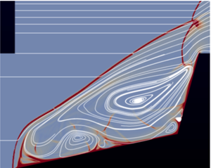
The features of flows located in the three characteristic regions labelled e, f and g in the map of figure 3 at condition A with  $\varLambda =1$ are brought out by the results shown in figure 8. The colour code is velocity magnitude and the sonic line has been drawn in white. The latter brings out the feature of these steady flows that there is a subsonic island in an otherwise supersonic flow except for the subsonic flow in the boundary layer and the separated region. Between these subsonic parts of the flow the supersonic shock train reaches all the way to the shoulder of cone 2, except in the case e, where it dissipates on the way. Figure 9 shows the same situations in the case when
 $\varLambda =0.5$.
Three views of the steady flows represented by locations (a–c) g, f and e in the map of figure 3, more precisely, ( $\theta _1$,
 $\theta _2$)
 $=$ (25
 $^\circ$, 54
 $^\circ$), (39
 $^\circ$, 68
 $^\circ$), (28
 $^\circ$, 85
 $^\circ$), respectively, with
 $\varLambda =1$. The colour is coded as velocity magnitude from
 $\textrm {blue} = 0$ through white to
 $\textrm {red} = 2720$ m s
 $^{-1}$. The white line is the sonic line. Note that the supersonic shock train reaches all the way to the cone 2 shoulder in the two left figures.

Three views of the steady flows represented by locations equivalent for  $\varLambda =0.5$ to (a–c) g, f and e in the map of figure 3, more precisely, (
 $\theta _1$,
 $\theta _2$)
 $=$ (25
 $^\circ$, 55
 $^\circ$), (40
 $^\circ$, 70
 $^\circ$), (33
 $^\circ$, 87
 $^\circ$), respectively. To see these locations relative to the
 $\varLambda =0.5$ unsteadiness boundary, refer to figure 21 right. The colour is coded as velocity magnitude from
 $\textrm {blue} = 0$ through white to
 $\textrm {red} = 2720$ m s
 $^{-1}$. The white line is the sonic line. Again, the supersonic shock train reaches all the way to the cone 2 shoulder in the two left figures.

4.2. Unsteady flows
In most of the unsteady regions of the  $\theta _1$–
 $\theta _2$ space, the unsteadiness is not very regular, as evidenced by visualization videos and pressure traces. Figure 10 shows three snapshots of flows at condition A and locations b, c and d in the map of figure 3. The corresponding pressure traces taken at the half-way point along the cone 1 generator are shown in figure 11 together with an example of a pressure trace from a steady flow. Despite the fact that, in all cases, the flows are started in a very abrupt manner, by specifying the free-stream conditions at the inflow boundary, with an initial condition of reduced pressure, the flow reaches steady state in
 ${\sim }1$ ms, or approximately 20 flow times. However, the time to steady state is much longer in flows at small
 $\theta _1$ and just below
 $\theta _2=\theta _{2d}$, as will be discussed in connection with the special unsteadiness observed by Kenworthy (Reference Kenworthy1978).
Three snapshot views during the unsteady flows at condition A and represented by locations (a–c) b, c and d in the map of figure 3. The colour is coded as temperature from  $\textrm {blue} = 300$ K through white to
 $\textrm {red} = 4000$ K.


Region a in the map of figure 3 is where close to periodic unsteadiness takes place. This is illustrated by the sequence of pseudo-schlieren images of a flow at condition A and  $\varLambda =0.5$, with (
 $\theta _1, \theta _2$)
 $=$ (12
 $^\circ$, 75
 $^\circ$) in figure 12. The nine panels in this sequence are separated by 40
 $\mathrm {\mu }$s from each other. The first and last of these are at approximately the same phase, so that the sequence covers approximately one cycle of the pulsating unsteadiness. The colour measures the magnitude of the density gradient from sky
 $\textrm {blue}=0$ to
 $\textrm {red}=\textrm {maximum}$. The white lines are streamlines, i.e. integral curves of the instantaneous velocity field. If this were a steady axisymmetric flow, the streamlines that are totally inside the domain would be closed curves. The fact that they can spiral into or out of a focus is because the flow is unsteady. It appears that the cycle is dominated by the generation, trapping, growth and spilling of a vortex ring. This mechanism will be analysed in more detail in the next section.
One cycle of the pulsating unsteadiness, condition A at location a in figure 3. The separation of the panels is approximately 35  $\mathrm {\mu }$s.

Figure 13 shows corresponding pressure traces taken at the half-way points of cone 1 and cone 2. These illustrate the almost periodic nature of the flow.
Pressure traces at the two half-way points on cone 1 (red) and cone 2 (green), condition A, location a in figure 3. The frequency is approximately 3 kHz, making the Strouhal number  $Sr=f d/U_\infty =0.176$, where
 $d$ is the base diameter of cone 2. Kenworthy's value for the somewhat different geometry of a spiked body with the same
 $\ell _1/d$ is 0.22.

A form of unsteadiness that does not occur in the results of our finite Reynolds-number computations may be illustrated by an inviscid computation at ( $\theta _1, \theta _2$)
 $=$ (12
 $^\circ$, 75
 $^\circ$) with
 $\varLambda =1$, otherwise condition A. This case is shown in figure 14. A shock train occurs in this flow too, showing that that is an inviscid feature. The shock train is quite unsteady and radiates acoustic noise toward the cone 2 shock. In our viscous computations of steady flows this unsteadiness is damped. The shock train unsteadiness is a feature related to the work of Tumuklu et al. (Reference Tumuklu, Theofilis and Levin2018) who found a number of coupled instability modes, which include the Kelvin–Helmholtz instability of the shear layer at the edge of the shock train. This form of unsteadiness is not part of our search for boundaries. (Note that this condition exhibits pulsating unsteadiness in viscous flow, where vorticity is generated at the cone 1 tip, see figure 12).
Result of an inviscid computation, otherwise at condition A, ( $\theta _1, \theta _2$)
 $=$ (12
 $^\circ$, 75
 $^\circ$) with
 $\varLambda =1$, showing an unsteady supersonic shock train radiating acoustic noise.

4.3. Kenworthy's unsteadiness at small  $\theta _1$ and $\theta _2<\theta _{2d}$


As was mentioned in the Introduction, Kenworthy (Reference Kenworthy1978) reported a small-amplitude periodic unsteadiness near ( $\theta _1, \theta _2$)
 $=$ (1
 $^\circ$, 50
 $^\circ$),
 $\varLambda =0.65$,
 $M_\infty =6$,
 $\gamma =1.4$,
 $Re=130\,000$. This was quite unusual, because nobody had previously observed unsteadiness for
 $\theta _2<\theta _{2d}$. It only occurred at this particular value of
 $\varLambda$, steady flow being observed at values below and above it. In order to understand this better, a computation was performed at the same conditions. Two panels of the development of this flow are shown in figure 15, one at 1.3 ms and one at 6 ms. The separation point in this flow moves very slowly toward the tip of cone 1. As it does so, the reattachment point moves up along cone 2. With this particular geometry the separation point reaches the cone 1 tip approximately at the same time as the reattachment point approaches the cone 2 shoulder. At that point the small-amplitude periodic unsteadiness starts. This is nicely brought out by the pressure traces at the two half-way points of the cones, see figure 16(a).
Results of a computation at ( $\theta _1, \theta _2$)
 $=$ (1
 $^\circ$, 50
 $^\circ$),
 $\varLambda =0.65$,
 $M_\infty =6$,
 $\gamma =1.4$,
 $Re=130\,000$, corresponding to the condition where Kenworthy observed oscillatory behaviour below the detachment angle. The frequency is 2.5 kHz. (a) at approximately 1.3 ms, (b) at approximately 6 ms.

(a) Pressure traces corresponding to the flow of figure 15 at the two half-way points of the cones, red: cone 1, green: cone 2. (b) Pressure traces for the case of condition A with  $\varLambda =1$ and (
 $\theta _1, \theta _2$)
 $=$ (10
 $^\circ , 50^\circ$) where a steady state is reached, albeit only after 140 flow times.

At first, the cone 1 sensor (red) lies upstream of the separation point, and the pressure there reaches a steady value. At the same time the cone 2 sensor (green) lies behind the almost normal cone 2 shock and registers close to Pitot pressure. At approximately 1.2 ms the separation point moves across the cone 1 sensor and the red trace rises slowly as the green trace falls. Then, at  ${\sim }5.4$ ms the oscillation begins. The amplitude is approximately the same as that observed by Kenworthy (4 % of Pitot pressure) which is small compared to the unsteadiness typically observed inside the loop (10 % to 100 %). The frequency of the green curve, which is at the same sensor location as Kenworthy's, corresponds to a Strouhal number
 $Sr=fd/U_\infty =0.118$ which compares well to the approximate value 0.110, determined from Kenworthy's geometry and flow speed, and
 $f$ measured from his pressure trace. Here,
 $d$ is the base diameter of cone 2.
A remarkable feature of this area of the map of figure 3 is that the time to reach a steady state (or the oscillatory one in Kenworthy's geometry) is very much longer than in the other steady-flow regions. It corresponds typically to more than 100 flow times. In our computations in this region of the map with  $\varLambda =1$ and 0.5, steady states are reached. An example is shown in figure 16 right.
5. Analysis of the pulsating unsteadiness
In order to gain more insight into the mechanism of the pulsating unsteadiness the case of condition D, with ( $\theta _1, \theta _2$)
 $=$ (1
 $^\circ$, 90
 $^\circ$) and
 $\varLambda =0.5$ is studied in detail here. Figure 17 shows a time sequence of pseudo-schlieren images with superimposed streamlines covering one cycle. As in the case of figure 12, the sequence starts in (a,b,c) with the cone 2 shock causing separation of the boundary layer on cone 1, thus lifting the vorticity generated at the tip of cone 1 off the surface and beginning to accumulate it in a vortex ring around the axis. The sense of the rotation (clockwise in this view) is such that the self-propagation direction of the vortex ring is to the left. Also, the vortex ring resists being stretched. Both of these help to trap the vortex ring. In (d,e,f), the shock has been pushed all the way to the cone 1 tip as the vortex ring grows. In (g,h,i) the vortex ring displaces the shock further upstream, thus opening up the sonic bottleneck between the cone 2 shoulder and the shock and allowing the vortex ring to escape over the cone 2 shoulder. The shock can now collapse onto cone 2 again, see (j,k,l), and the cycle repeats.
Time sequence of panels separated by 40  $\mathrm {\mu }$s at condition D with (
 $\theta _1, \theta _2$)
 $=$ (1
 $^\circ$, 90
 $^\circ$) and
 $\varLambda =0.5$.

It seems, therefore, that the unsteadiness hinges on the accumulation of the vorticity, generated at the cone 1 tip by the no-slip condition, into a vortex ring. Thus, if the no-slip condition is removed, e.g. either by an inviscid computation or by a viscous, heat-conducting computation in which the no-slip and cold-wall boundary conditions are replaced by no shear and no heat flux conditions, the unsteadiness should disappear. Figure 18 shows the results of such computations with otherwise the same conditions as in figure 17. Clearly, the removal of the no-slip condition removes the unsteadiness and almost identical steady flows result.
In the case ( $\theta _1, \theta _2$)
 $=$ (1
 $^\circ$, 90
 $^\circ$) with
 $\varLambda =0.5$, (a) shows the result of an inviscid computation. (b) shows what happens if, in a viscous heat-conducting flow the no-slip and cold-wall conditions are replaced by setting the wall-normal components of the gradients of temperature and wall-parallel velocity equal to zero, i.e. setting the wall shear stress and heat flux to the wall to zero.

The removal of the no-slip condition also removes the vorticity source at the tip of cone 1 and, in view of our understanding of the vortex ring mechanism, it is therefore not surprising that it removes the unsteadiness. It is interesting to observe that one could generate vorticity in an otherwise inviscid flow by the baroclinic torque in a curved shock wave by making the tip of cone 1 blunt. The vorticity downstream of a curved shock wave in a steady free stream is given by, see Hayes & Probstein (Reference Hayes and Probstein1959),
 \begin{equation} \frac{\omega r}{U}=\cos{\beta}\frac{(1-\varepsilon)^2}{\varepsilon}, \end{equation}
where  $\omega$ is the vorticity,
 $r$ is the shock wave radius of curvature,
 $U$ is the free-stream velocity,
 $\beta$ is the shock angle and
 $\varepsilon$ is the inverse density ratio across the shock. We want the vorticity to be in the MHz range, and with our conditions, that means that
 $r$ should be roughly 3 mm. Such a bow shock could be generated by a nose bluntness of approximately 2 mm radius. This idea was tested by computing inviscid flow exactly as in the case shown in figure 18(a), with the sole difference that the tip of cone 1 is cut off to make it blunt. The result is a flow with pulsating unsteadiness, one cycle of which is shown in a time sequence in figure 19. The similarity between the time sequences in figures 17 and 19 shows that the occurrence of pulsating unsteadiness is independent of the manner in which the vorticity is generated.
Time sequence of results of an inviscid computation with ( $\theta _1, \theta _2$)
 $=$ (1
 $^\circ$, 90
 $^\circ$) and
 $\varLambda =0.5$, otherwise at condition D with a blunt nose tip on cone 1.

The pressure traces of the viscous sharp and inviscid blunt flows are shown in figure 20. The pressure traces of the blunt-tip inviscid flow are not as regular as those of the viscous one, and take a little longer to settle in. This is why the period from 2 to 5 ms is shown for that case. One of the differences between the two flows is the duty cycle of the vorticity production rate. In the viscous case, the rate is reduced somewhat when the shock is pushed forward to the cone 1 tip. In the blunt case the rate of production goes practically to zero at that time.
Pressure traces at the half-way points on cone 1 (red) and cone 2 (green) at condition D, ( $\theta _1, \theta _2$)
 $=$ (1
 $^\circ$, 90
 $^\circ$) with
 $\varLambda =0.5$. (a) Viscous, sharp tip. (b) Inviscid, blunt tip. In both cases the frequency is approximately 1.7 kHz making the Strouhal number
 $Sr=f d/U_\infty = 0.26$.

These examples show that the pulsating unsteadiness is essentially an inviscid phenomenon. If vorticity is produced at a suitable rate near the tip of cone 1, pulsating unsteadiness is enabled in otherwise suitable conditions. It follows that, although the steady flows are Reynolds-number dependent, the unsteadiness boundaries are not. It should be pointed out that the exercise performed in this section in the case of condition D was repeated at two other condition A angle pairs with the same conclusions.
6. The unsteadiness boundary
Many of the examples used to illustrate the results were taken from conditions A and D. It remains to present the results for all the conditions computed. To this end, figure 21 shows the unsteadiness boundaries for conditions A, B, C and D, for  $\varLambda =1$ and 0.5. At this point we note that the boundary for condition A’ was found to be indistinguishable from that of condition A for both values of
 $\varLambda$ and is therefore not shown. This supports the conclusion that the unsteadiness boundaries are essentially an inviscid phenomenon. The lower branch of the loops enclosing the unsteady regions in each case asymptotes to
 $\theta _2=\theta _{2d}$ at small
 $\theta _1$.
Unsteadiness boundaries in the  $\theta _1$–
 $\theta _2$ plane; (a)
 $\varLambda =1$, (b)
 $\varLambda =0.5$. The short black lines indicate the values of the second-cone detachment angle
 $\theta _{2d}$. Error bars indicating the typical uncertainties in the determination of the boundaries are shown on the upper and lower branches for conditions A and B.

The upper branch may be understood by taking condition A,  $\varLambda =1$, and following a line at
 $\theta _1=30^\circ$ from the steady region below
 $\theta _2=\theta _{2d}$ upward. In this steady region, the cone 2 shock is relatively weak and propagates a separation shock forward to a stable position, forming a separation bubble followed by a supersonic shock train. As
 $\theta _2$ is increased across the lower branch, the cone 2 shock strength increases dramatically, causing the separation to move forward and lifting the vorticity off the surface, accumulating it into a trapped vortex ring, and so setting off the unsteadiness. As
 $\theta _2$ is increased, the cone 2 shock is pushed upstream, thus increasing the area of the sonic bottleneck until at the upper branch it allows vorticity to escape as fast as it is produced at the cone 1 tip. Support for this effect is provided by the fact that the upper branches lie at higher values of
 $\theta _2$ in the case of
 $\varLambda =0.5$ than for
 $\varLambda =1$, because, for fixed
 $\theta _2$, the distance between the cone 2 shoulder and the cone 2 shock is approximately proportional to
 $\ell _2$, so that the bottleneck area is smaller for
 $\varLambda =0.5$. Thus, the transition back to steady flow requires a larger value of
 $\theta _2$ when
 $\varLambda =0.5$. Figure 21 shows a few representative error bars. These reflect the density with which the computations covered the
 $\theta _1$–
 $\theta _2$ space and show that the upper branch was not as well resolved as the lower.
The dominance of the second-cone detachment angle suggests that the stretched variable
 \begin{equation} \eta_2=\frac{\theta_2-\theta_{2d}}{{\rm \pi}/2-\theta_{2d}} \end{equation}
that has already been used effectively by Hornung, Martinez Schramm & Hannemann (Reference Hornung, Martinez Schramm and Hannemann2019) should be tried. Accordingly, figure 22 shows a plot of the same information in  $\theta _1$–
 $\eta _2$ space. This graph shows that the lower branch collapses almost onto a unique curve in these coordinates and that the upper branches of the hypersonic cases A, B and (marginally hypersonic) C fall within the error bars of a single curve for each of
 $\varLambda =1$ and 0.5. If we accept that, within the bounds of our investigation, the unsteadiness boundaries are inviscid in nature and therefore Reynolds-number independent, (2.4) may be written for hypersonic flow (i.e. excluding case D) as
 \begin{equation} Q=Q(\theta_1,\eta_2,\varLambda). \end{equation}
Unsteadiness boundaries with  $\theta _2$ scaled to
 $\eta _2$. (a)
 $\varLambda =1$, (b)
 $\varLambda =0.5$.

7. Conclusions
A computational parameter study of the supersonic axisymmetric flow over double cones was conducted, with the aim to find the boundaries within which such flows are unsteady. The study was limited to laminar boundary layer flow. While past research on the unsteadiness concentrated on the case when  $\theta _1$ is small and covered the length ratio
 $\varLambda$ in detail, the emphasis here was on covering the
 $\theta _1$–
 $\theta _2$ space in detail at only two values of
 $\varLambda$. At each of five free-stream conditions, chosen to span a range of values of the cone 2 shock detachment angle, the unsteadiness boundary in this space was found to be a loop with a lower
 $\theta _2$ branch dominated by the detachment angle, and an upper
 $\theta _2$ branch with a maximum
 $\theta _1$ between them.
The features of the steady and unsteady flows in different parts of the  $\theta _1$–
 $\theta _2$ space were described and the pulsating unsteadiness was analysed in detail. The steps in the time development of the cycle are: vorticity generation at the cone 1 tip, its accumulation in a vortex ring around the axis, forward displacement of the shock by the vortex ring growth, permitting its escape around the cone 2 shoulder. By replacing the no-slip vorticity production of the viscous flow by the baroclinic torque within a curved bow shock in an inviscid flow with blunt tip, it was shown that the unsteadiness is independent of the method of vorticity production and is essentially an inviscid phenomenon.
The special case of a small-amplitude unsteadiness observed by Kenworthy (Reference Kenworthy1978) at small  $\theta _1$ and
 $\theta _2<\theta _{2d}$ could be reproduced computationally. This occurs only for a particular small range of
 $\varLambda$. In this region of
 $\theta _1$–
 $\theta _2$ space the time to reach steady state is extraordinarily long, requiring more than 100 as compared with
 ${\sim }20$ flow times in the other steady-flow regions.
By scaling  $\theta _2$ in a stretched coordinate involving the detachment angle, it was shown that, for the hypersonic case, the unsteadiness boundary could be expressed in terms of only three independent dimensionless variables within the bounds and within the uncertainties of the investigation.
Funding
This work was partially supported by the US Air Force Office of Scientific Research under contract AFOSR FA9550-15-1-0288, P.I.: J.M. Austin, program officer: I.A. Leyva.
Declaration of interests
The authors report no conflict of interest.



