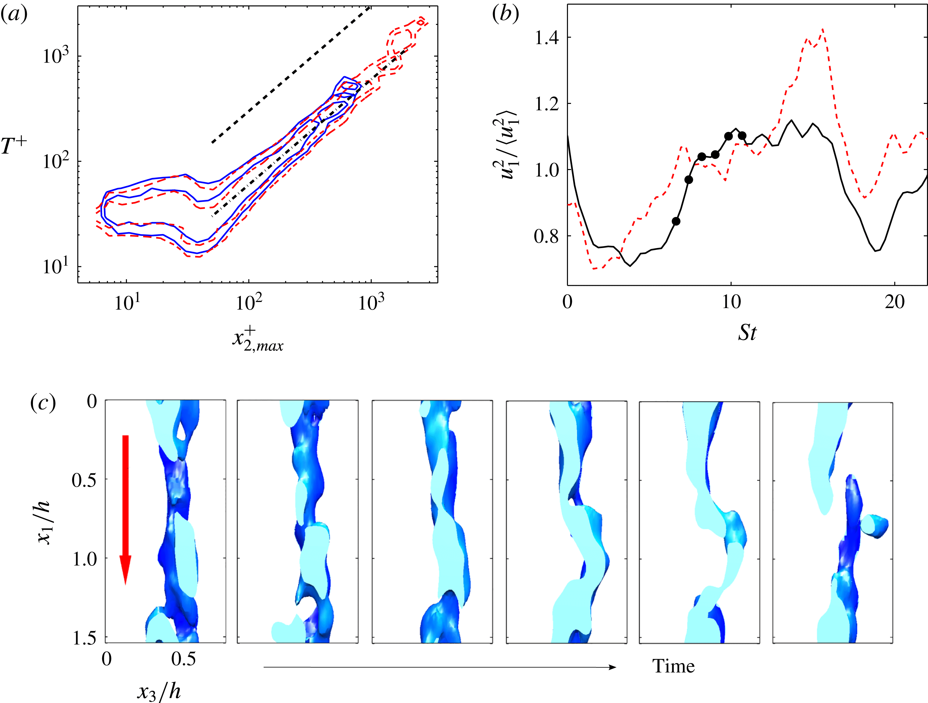
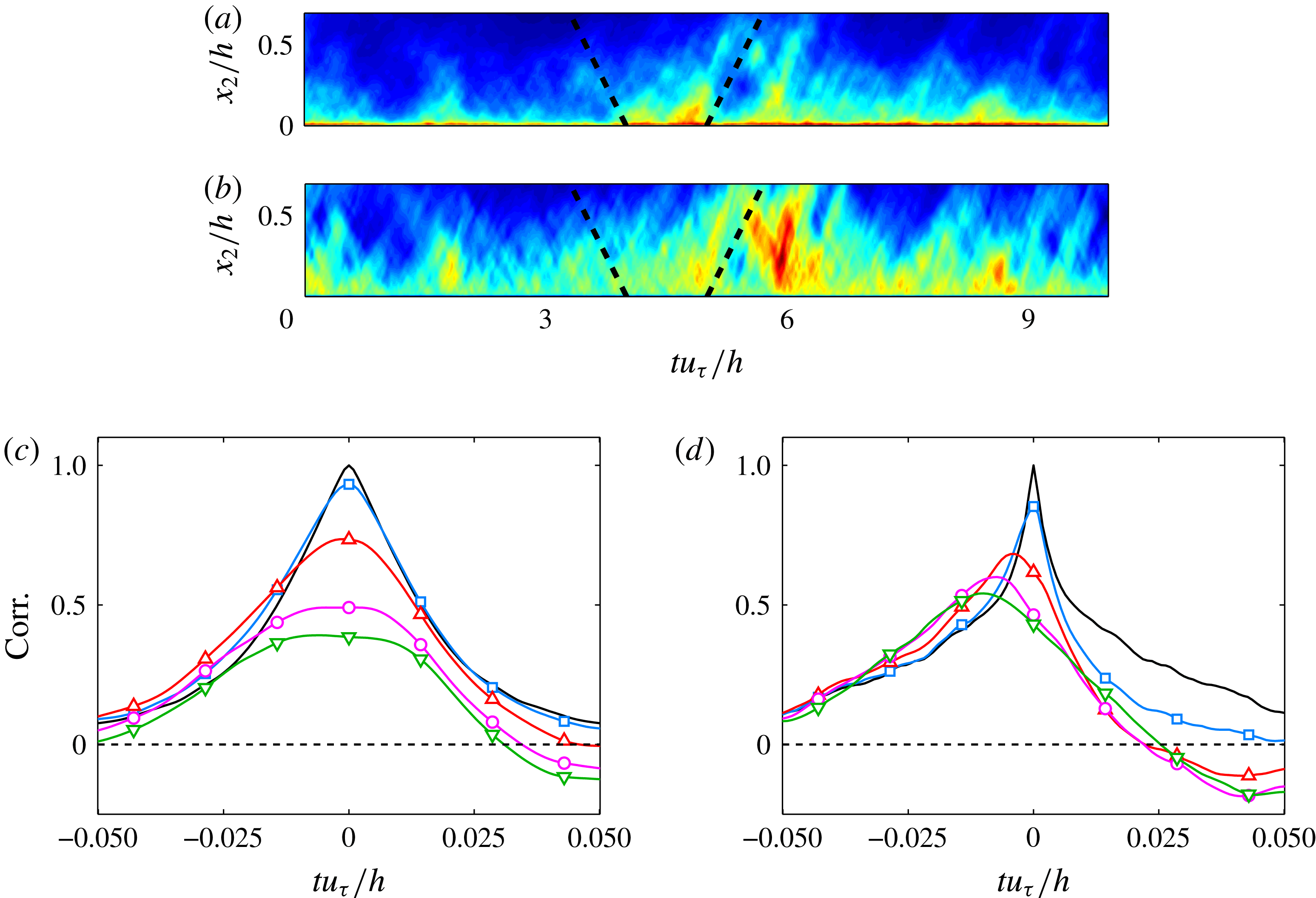
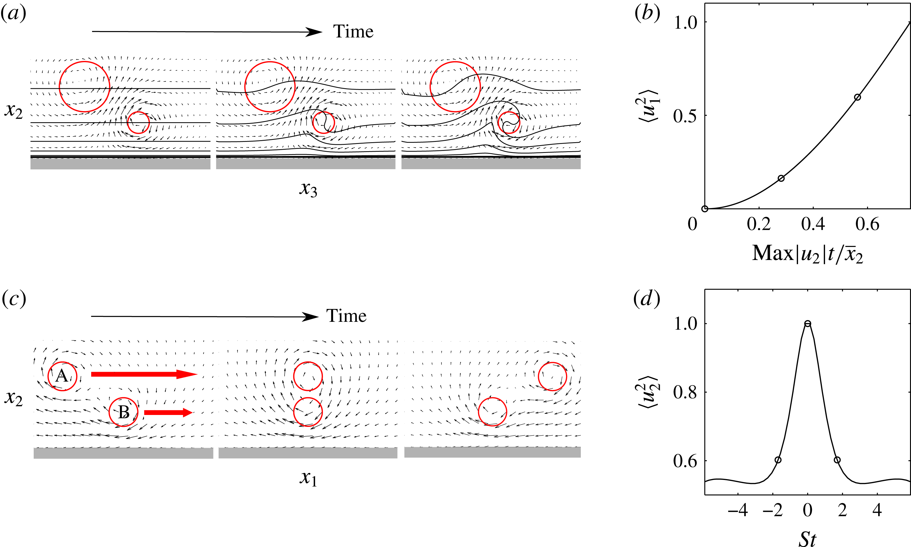
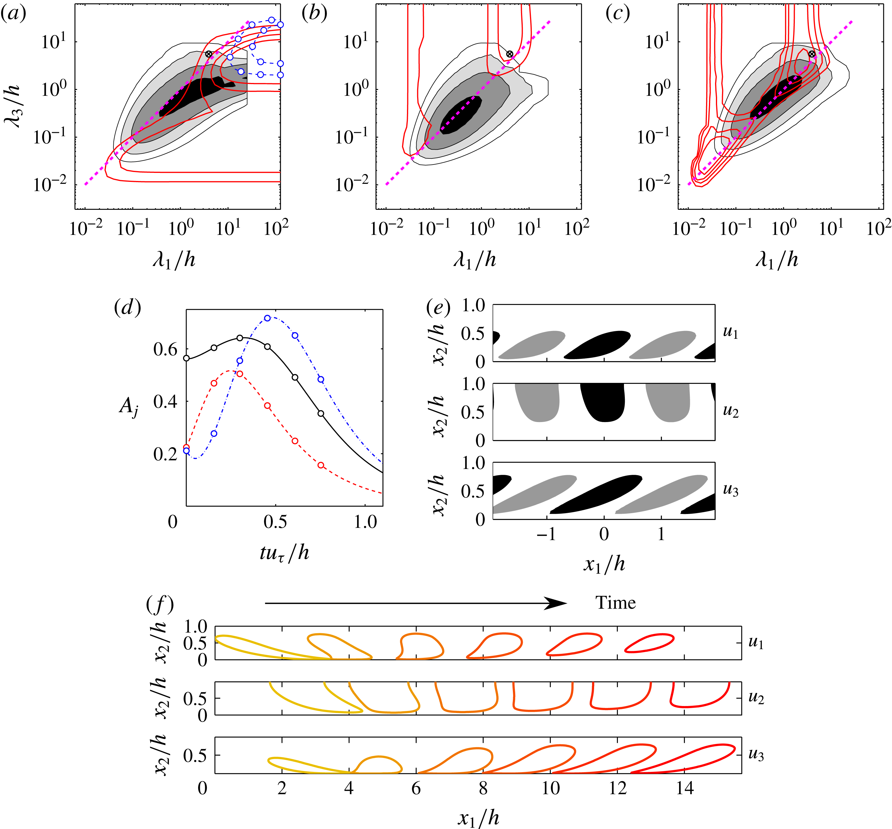
1 Introduction
Turbulence is often treated as a random process in which important questions are posed in terms of statistics. In addition, whenever the equations of motion are explicitly invoked, they are often seen as ‘filters’ modifying the effect of random noise (Landau & Lifshitz Reference Landau and Lifshitz1959). This article takes the alternative view that randomness is an admission of ignorance that should be avoided whenever possible (Voltaire Reference Voltaire1764), and that turbulence is a dynamical system which satisfies the Navier–Stokes equations and can be treated deterministically over time intervals and spatial domains that, even if limited, are of theoretical and practical relevance. Specifically, we will be interested in whether the description of the flow can be simplified by decomposing it into ‘coherent’ structures that can be extracted by observation and predicted from theoretical considerations. In this sense, we continue a tradition of ‘eddy chasing’ that, as we shall see, has been pursued in the past few decades with as much vigour as the purely statistical approach.
However, any attempt to simplify complexity has to be treated with caution, because it usually implies neglecting something that may be important. For example, the motion of the molecules in a gas cannot be simplified without cost. Thermodynamics follows simple rules, but only at the expense of hiding the instantaneous motion of individual molecules, preventing us from building ‘Maxwell demons’. This does not mean that simplification should not be pursued. It may be the only way of making the system tractable, but it should be undertaken with proper care to distinguish between what is important for the system and what is convenient for us.
The structural view of turbulence is based on the hope that at least part of its dynamics can be described in terms of a relatively small number of more elementary processes than the full Navier–Stokes equations.
There are several ways of approaching this goal. Reduced-order models seek to project the equations of motion onto a smaller set of variables that approximate the solution in some global sense, typically a linear subspace or a few Fourier modes (see, for example, Rowley & Dawson Reference Rowley and Dawson2017). The key word in this sentence is ‘global’, and becomes less justified as the system becomes more extended. Consider a turbulent boundary layer over a wing, where the wall-parallel dimensions can be several hundred times the flow thickness. We can expect to find several thousands of ‘largest’ eddies in such systems, many of which will be so far apart from each other as to be essentially independent. Global definitions fail in those cases, essentially because they treat together unrelated quantities.
Our approach will rather be to acknowledge that the evolution of the flow is largely local, and to look for solutions that are intense enough to evolve on their own, relatively independently from other solutions far away. We will refer to these putative solutions, different from global modes, as ‘coherent structures’. The two outlooks are in some ways similar to the wave and particle representations in quantum mechanics.
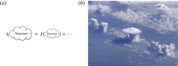
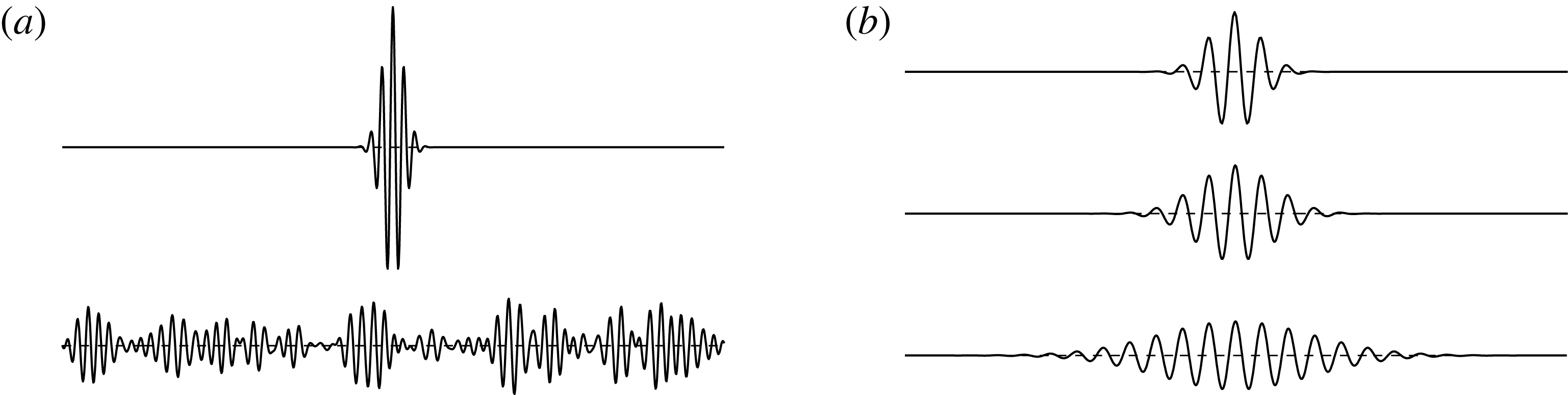
It would be useful for our purpose that structures, if they exist, depend predominantly on other structures and on themselves, at least for some time, with relatively small contributions from the ‘unstructured’ background (see figure 1 a). Such ‘self’-dependence suggests several properties that structures should possess. In the first place, they should be strong with respect to their surroundings and have some dynamics of their own, e.g., a vortex would do, but a blob of red dye may not. They should also be relevant enough to the flow not to be considered trivial, even if it should be noted that relevance is a subjective property more related to the observer than to the flow, and that it depends on the application. For example, a strong Kolmogorov-scale vortex is not very relevant to the overall energy balance of the flow, but it might be important for the behaviour of a premixed flame. Finally, to be useful, structures should be observable, or at least computable.
These requirements generally imply that coherent structures should either be ‘engines’ that extract energy from some relevant forcing, ‘sinks’ that dissipate it, or ‘repositories’ that hold energy long enough to be important for the general energy budget of the flow.
It follows from the above arguments that the first questions to be addressed should be whether structures satisfying these requirements are possible, which simplifications they imply, and whether the parts that can be described structurally are relevant for the flow as a whole.
(a) Conceptual sketch of a possible definition of coherent structure. The remainder implied by the dots at the end of the equation is assumed to be ‘small’. (b) Structures need not describe the full flow to be useful (image courtesy of NASA).

In common with other models, structural descriptions should not conflict with known evidence, but they should not necessarily be required to explain all the evidence. They may be useful even if part of the flow, or even most of it, is structureless. For example, the tall cumulus cloud at the centre of figure 1(b) will probably result in a strong shower. This is a useful local prediction, even if most of the rest of the sky is clear.
Turbulence, and in particular wall-bounded turbulence, is a complex chaotic system with many degrees of freedom, with some superficial similarity to the molecular description of a gas. In fact, entropy considerations have been used to motivate the direction of the turbulence cascade (Onsager Reference Onsager1949; Kraichnan Reference Kraichnan1971). The evolution of the Fourier coefficients of inviscid turbulence with a bounded set of wavenumbers,
 $k$
, can be written as a Liouville system that conserves volume in phase space, and which can therefore be expected to evolve towards a maximum-entropy state in which energy is equipartitioned over the wavenumbers. In three-dimensional flows, this would result in an energy spectrum,
 $E(k)\sim k^{2}$
, in which most of the energy is in the highest wavenumbers, simply because the surface of a sphere increases with its radius, and Fourier shells with larger wavenumbers contain more Fourier modes. In this view, the three-dimensional energy cascade of the viscous Navier–Stokes equations is an attempt by the flow to fill the more numerous wavenumbers at small scales, frustrated by the vigorous viscous dissipation at those scales.
This would appear to argue against the possibility of representing turbulence in terms of structures that are ‘coherent’ enough to be identified as ‘objects’, because any amount of organisation reduces entropy, but there are several reasons why this is not true. The first one is that turbulence is very far from equilibrium. Even assuming statistical stationarity, and disregarding viscosity in the inertial range, energy flows on average from its injection at large scales to dissipation at small scales. The implied model is not so much an equilibrium gas, but one in which heat flows from a hot wall to a cold wall. A succinct discussion of the relation between non-equilibrium systems and macroscopic structures is Prigogine (Reference Prigogine1978).
Another reason is that even equilibrium thermodynamic systems fluctuate, although the relative magnitude of the fluctuations decreases exponentially with the number of degrees of freedom. This number is typically large in turbulence,
 $N_{dof}\sim Re^{9/4}$
for a Reynolds number
 $Re$
of the energy-containing eddies, but much smaller than in thermodynamics. Even for a ‘high’
 $Re=10^{5}$
,
 $N_{dof}\approx 10^{11}$
is ten or twelve orders of magnitude less than the typical number of molecules in a gas.
But the most compelling reason is that, in the far-from-equilibrium state of Kolmogorov (Reference Kolmogorov1941) turbulence, all degrees of freedom are not equivalent and that, when speaking about structures, we are typically only interested in a small fraction of modes. The probability of random fluctuations is controlled by their effect on the entropy (Landau & Lifshitz Reference Landau and Lifshitz1958), which depends on the number of degrees of freedom involved, but their practical significance is linked to the energy or to the Reynolds stresses that they contain. In Kolmogorov (Reference Kolmogorov1941) turbulence, energy is associated with a relatively small number of large-scale degrees of freedom, which are therefore relatively free to fluctuate strongly. These large-scale fluctuations also tend to maintain coherence over long times which are at least of the order of their eddy turnover.
We will centre on identifying and characterising such coherent structures. There are many reasons why we may want to do so, although some of them are probably more relevant to the kind of understanding that appeals to the human mind than to the flow dynamics. To retain some connection with applications, and although the issue of control will not be addressed explicitly in this paper, the question of building a ‘Maxwell demon’ to manipulate the energy flux in turbulence using a structural representation will always be in the background of our discussion. The most familiar consequence of thermodynamics is that we cannot extract work from the thermal motion of the molecules in an equilibrium system (Earman & Norton Reference Earman and Norton1998), but we have argued that equilibrium thermodynamics is not applicable here, and anybody who has flown a glider in thermals, or manoeuvred a sail boat, knows that it is possible to extract work from turbulence by taking advantage of its structures. The literature on turbulence control is far too extensive to be reviewed here, but some idea of the flavour of the discussions on the relevance of structures for control can be gained from Lumley, & Blossey (Reference Lumley and Blossey1998), for wall-bounded flows, or Choi, Jeon & Kim (Reference Choi, Jeon and Kim2008), for free-shear flows.
Coherent structures are often found in transitional flows, where they are typically described as arising from linear modal instabilities of the base laminar flow. This modal origin gives rise to well-ordered patterns and wavetrains for which there is a rich and well-developed theory. A classical description of this line of work is Drazin & Reid (Reference Drazin and Reid1981). However, we are interested here in the asymptotic state of turbulence at high Reynolds numbers, far from transition, and the ordered patterns of linear instability are soon lost to nonlinearity and to the chaotic interaction of the large number of degrees of freedom. Part of the goal of this paper is to enquire whether transitional structures play any role in fully developed turbulence, in the hope that linearly unstable growth may provide a framework on which to ‘hang’ nonlinearity, even at the cost of considering the flow in some smoothed or averaged sense.
Several relatively new developments help us in this task. The first one is the realisation that modal growth is not the only possible way in which perturbations can grow linearly. When the evolution operator is non-normal, i.e. when it cannot be expanded in a set of mutually orthogonal eigenfunctions, even completely stable perturbations can grow substantially before they eventually decay. The linearised Navier–Stokes equations are highly non-normal for several reasons, and the modal instabilities of individual eigenfunctions give a very partial view of their behaviour. A modern account of these techniques is Schmid & Henningson (Reference Schmid and Henningson2001), and we will discuss this approach in more detail in § 6.
Another modern development is the computation of fully nonlinear invariant solutions of the Navier–Stokes equations, either permanent waves or relative periodic orbits, starting with Nagata (Reference Nagata1990). These solutions have often been described as ‘exact coherent structures’ (Waleffe Reference Waleffe2001), which they strongly resemble (Jiménez et al. Reference Jiménez, Kawahara, Simens, Nagata and Shiba2005), but the similarity is only partial. In the first place, the known solutions are typically restricted to a single structure in a ‘minimal’ flow unit and, although it has been shown that the temporally chaotic flow in such minimal units shares many properties with turbulence in extended systems (Jiménez & Moin Reference Jiménez and Moin1991), it fails in important aspects. Most crucially, minimal units are essentially single-scale systems, which cannot reproduce the multiscale interactions of high-Reynolds-number flows. Most of the above discussion on entropic behaviour does not carry over to minimal units and, although there is a general feeling that it should be possible to ‘synthesise’ large-scale turbulence from an ensemble of minimal units of different size, the details remain unclear. Invariant solutions are typically unstable, and are not expected to be found as such in real flows. This is probably helpful in connection with their role as building blocks for multiscale solutions, because it prevents the system from getting ‘stuck’ in an attractor that is too simple to be considered turbulent. It has often been noted that an invariant solution is a fixed point (or a permanent orbit) in the space of possible flow configurations, and that the system could spend a relatively large fraction of the time in its neighbourhood as it ‘pinballs’ among different solutions. The properties of invariant solutions could therefore be important for the overall flow statistics (Ruelle Reference Ruelle1978; Jiménez Reference Jiménez1987b ; Cvitanović Reference Cvitanović1988), even in the context of fully developed turbulence. A modern review of this point of view is Kawahara et al. (Reference Kawahara, Uhlmann and van Veen2012).
The third modern development that will help us in our goal is the direct numerical simulation (DNS) of turbulence, which, although initially restricted to low Reynolds numbers (Rogallo Reference Rogallo1981; Kim, Moin & Moser Reference Kim, Moin and Moser1987), was later extended to increasingly higher values. Simulations today span a range of Reynolds numbers that overlaps the range of most experiments, and which often exceeds that of the experiments for which reasonably complete measurements are possible. The main advantage of simulations is that they are ‘observationally perfect’. This is, in fact, the reason for their high cost. The equations have to be simulated in full to properly represent the flow and, although some information can be discarded during postprocessing, it is impossible to restrict direct simulations to partial solutions. As a consequence, simulations potentially provide the answer to ‘any’ question, and allow us to see the Navier–Stokes equations as a dynamical system. It is routinely possible to compute and, up to a point, to store, temporally and spatially resolved sequences of three-dimensional fields of any required variable. These sequences reside in computer storage, and can be interrogated forwards and backwards in time with any desired technique, and as often as required. The pacing item is no longer how to obtain answers, but how to pose questions. Turbulence research, in common with other sciences at some point in their development, has changed from a subject driven by the need for good data, to one driven by the need for new ideas.
Before continuing, it is useful to make explicit the distinction between eddies and structures, which are often treated as equivalent but are conceptually very different (Adrian & Moin Reference Adrian and Moin1988). In the sense used in this paper, eddies are statistical representations of the most probable state of the flow, while structures need dynamics. Going back to the example in figure 1(b), the statistically most probable cloud in most weather patterns is unlikely to be an active storm cumulus, but cumuli are locally very significant.
This article is organised in three broad sections. Section 3 addresses the classical view of wall-bounded turbulence, considered independently of whether coherent structures exist or not. Sections 4 and 5 review what is meant by structures, how they are detected, and what is the experimental evidence for their existence, and § 6 summarises some of the models that have been developed to explain them. Two appendices collect details of the methods of analysis, and a short initial § 2 explores the interplay between coherence and chaos. Roughly speaking, the three parts of the paper deal with what happens, how it happens, and why it happens. None of them should be considered a full review, and readers are encouraged to consult the original references provided. Most people will feel that important references are missing. This is unfortunately unavoidable if an article as broad as this one is to stay within the size limitations. I have tried to incorporate most points of view, albeit sometimes briefly, but I am obviously biased towards the particular one that I have tried to make explicit in this introduction. Mostly, I have been interested in enquiring how the different strands of research are related to each other, and what facts and observations should be taken into account by any future explanation. I also apologise for using mostly data from our group. I have them more readily available than those of others, and the original publications make the necessary comparisons.
2 An example of coherence in a chaotic system
Before moving to the study of coherent structures in turbulence, it might be useful to clarify the idea of coherence in a simpler system. The equations
 $$\begin{eqnarray}\displaystyle \left.\begin{array}{@{}c@{}}\text{d}\unicode[STIX]{x1D703}_{1}/\text{d}t=\unicode[STIX]{x1D70E}(\unicode[STIX]{x1D703}_{2}-\unicode[STIX]{x1D703}_{1}),\\ \text{d}\unicode[STIX]{x1D703}_{2}/\text{d}t=(\unicode[STIX]{x1D70C}-\unicode[STIX]{x1D703}_{3})\unicode[STIX]{x1D703}_{1}-\unicode[STIX]{x1D703}_{2},\\ \text{d}\unicode[STIX]{x1D703}_{3}/\text{d}t=\unicode[STIX]{x1D703}_{1}\unicode[STIX]{x1D703}_{2}-Q\unicode[STIX]{x1D703}_{3},\end{array}\right\} & & \displaystyle\end{eqnarray}$$
were introduced by Lorenz (Reference Lorenz1963) as a model for thermal convection in a two-dimensional box heated from below. The parameter
 $\unicode[STIX]{x1D70E}$
is the Prandtl number,
 $\unicode[STIX]{x1D70C}$
is proportional to the Rayleigh number, and
 $Q$
is related to the box aspect ratio. The components of the state vector
 $\unicode[STIX]{x1D73D}=[\unicode[STIX]{x1D703}_{j}],\,j=1\ldots 3$
represent, respectively, the fluid velocity and the horizontal and vertical temperature gradients. The solutions to (2.1) have been studied extensively, often for the parameters
 $\unicode[STIX]{x1D70E}=10$
,
 $\unicode[STIX]{x1D70C}=28$
and
 $Q=8/3$
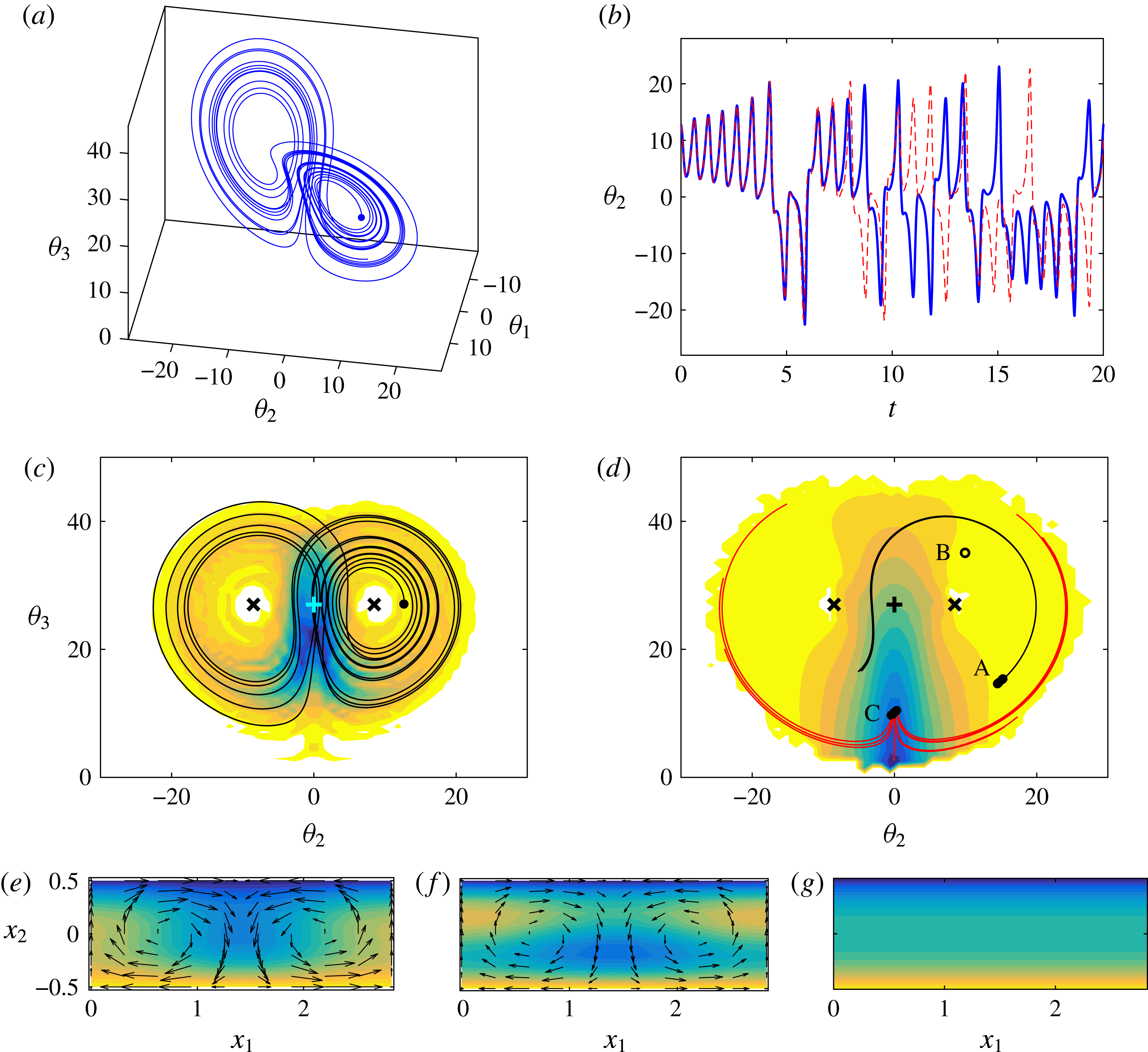
used in this section (e.g., see Bergé, Pomeau & Vidal Reference Bergé, Pomeau and Vidal1984, § VI, for many of the results cited below). They are chaotic, and trajectories collapse to a quasi-two-dimensional fractal attractor of dimension approximately 2.06. A sample trajectory is shown in figure 2(a), and the corresponding evolution of the horizontal temperature gradient is in figure 2(b).
Properties of the solutions of the Lorenz system (2.1) for
 $\unicode[STIX]{x1D70E}=10,\,\unicode[STIX]{x1D70C}=28,\,Q=8/3$
. (a) Sample trajectory in the three-dimensional state space, starting from the initial condition marked as a solid circle. (b) Temporal evolution of the horizontal velocity gradient,
 $\unicode[STIX]{x1D703}_{2}$
: ——, as in (a); - - -, with initial conditions displaced by
 $10^{-3}$
in all three variables. (c) The shaded contours are the joint p.d.f. of the two temperature gradients,
 $\text{p.d.f.}(\unicode[STIX]{x1D703}_{2},\unicode[STIX]{x1D703}_{3})/\text{p.d.f.}_{max}=0.033(0.066)1$
, increasing from light to dark. The solid line is the initial part of the trajectory in (a).
 $+$
, Equilibrium saddle;
 $\times$
, equilibrium foci. (d) The shaded contours are the leading short-time Lyapunov exponent,
 $L_{\unicode[STIX]{x1D70F}}=0.1(1)11.1$
, increasing from light to dark, with
 $\unicode[STIX]{x1D70F}=0.3$
. The solid lines are sets of ten trajectories each, randomly initialised within two neighbourhoods
 $(|\unicode[STIX]{x1D739}\unicode[STIX]{x1D73D}|\leqslant 0.5)$
centred on the attractor. The trajectories starting near point ‘A’ barely diverge over the time displayed
 $(t=0.5)$
. Those starting near ‘C’ bifurcate randomly towards one of the foci. (e–g) Flow configuration for the three states marked by letters in (d). The shaded background is the temperature, increasing from dark to light. Arrows are the velocity field. Units are arbitrary, but the scale is preserved among the three panels. (e) Point ‘A’,
 $\unicode[STIX]{x1D73D}=[15,15,15]$
. (f) ‘B’,
 $[10,10,35]$
. (g) ‘C’,
 $[0,0,15]$
.

Figure 2(b) includes a second simulation in which the initial conditions have been slightly displaced with respect to the first one. Both solutions eventually drift apart, and this characteristic sensitivity of chaotic systems to small perturbations has often been used to argue that individual trajectories are not relevant to problems such as turbulence, which should primarily be studied statistically (see Pope Reference Pope2000, § 3). The objects of interest in those cases would not be trajectories such as those in figure 2(a,b), but long-term probability density functions (p.d.f.) such as the one in figure 2(c).
However, inspection of figure 2(a–c) suggests a more nuanced interpretation. There are three unstable equilibrium points: two foci at
 $\unicode[STIX]{x1D703}_{2}\approx \pm 15$
, where the p.d.f. is minimum, and a saddle at
 $\unicode[STIX]{x1D703}_{2}=0$
where it is maximum. The trajectories evolve on two time scales: a short one,
 $T\approx 0.9$
, over which the state vector circles fairly regularly one of the foci, and a longer irregular one over which it switches from one focus to the other. Only the latter behaviour is chaotic. The short-time evolution is essentially deterministic, and can be considered coherent in the sense discussed in the introduction, although embedded in a chaotic system which has to be treated statistically over longer times.
This idea of coherence can be quantified. The sensitivity of the system to a linearised infinitesimal perturbation of the initial conditions,
 $\unicode[STIX]{x1D739}\unicode[STIX]{x1D73D}(0)=[\unicode[STIX]{x1D6FF}\unicode[STIX]{x1D703}_{j}(0)]$
, can be measured over a time interval
 $\unicode[STIX]{x1D70F}$
by the leading short-time Lyapunov exponent,
 $$\begin{eqnarray}L_{\unicode[STIX]{x1D70F}}=\unicode[STIX]{x1D70F}^{-1}\max _{\unicode[STIX]{x1D6FF}\unicode[STIX]{x1D703}(0)}\log \left(\Vert \unicode[STIX]{x1D739}\unicode[STIX]{x1D73D}(\unicode[STIX]{x1D70F})\Vert /\Vert \unicode[STIX]{x1D739}\unicode[STIX]{x1D73D}(0)\Vert \right),\end{eqnarray}$$
where the maximum is taken over all possible orientations of
 $\unicode[STIX]{x1D739}\unicode[STIX]{x1D73D}(0)$
, and which reflects the exponential growth of the norm of the perturbation. This short-time exponent depends on the initial conditions, and any given state can be considered predictable for times such that
 $\unicode[STIX]{x1D70F}L_{\unicode[STIX]{x1D70F}}\lesssim 1$
. In addition, an overall measure of the predictability of the system is the global Lyapunov exponent,
 $$\begin{eqnarray}L_{\infty }=\lim _{\unicode[STIX]{x1D70F}\rightarrow \infty }L_{\unicode[STIX]{x1D70F}},\end{eqnarray}$$
which is typically independent of the initial conditions. In this global sense, any system with a positive Lyapunov exponent should be treated statistically, at least for times longer, on average, than
 $\unicode[STIX]{x1D70F}\gtrsim 1/L_{\infty }$
. It can be shown that
 $L_{\infty }\approx 0.9$
for the case in figure 2(a), suggesting that no useful predictions can be done for times longer than
 $\unicode[STIX]{x1D70F}\approx 1$
.
However, the global Lyapunov exponent hides a wide variation in the predictability of the individual states of the system. This is seen in figure 2(d), which maps the short-time exponent, for
 $\unicode[STIX]{x1D70F}=0.3$
, as a function of the initial conditions on the attractor. It ranges from
 $L_{\unicode[STIX]{x1D70F}}\approx 0.1$
in the neighbourhood of the foci, to
 $L_{\unicode[STIX]{x1D70F}}\approx 10$
near the central saddle, implying a range of predictability times from
 $\unicode[STIX]{x1D70F}=10$
to
 $\unicode[STIX]{x1D70F}=0.1$
. This is confirmed by the two sets of trajectories included in figure 2(d). Both sets are initialised with the same initial scatter, but the trajectories originating near the low-
 $L_{\unicode[STIX]{x1D70F}}$
point ‘A’ complete an almost full orbit around their focus without any visible scatter, while those initialised around point ‘C’, near the saddle, exit randomly towards one or the other wing of the attractor.
The flow structures associated with different points of state space are displayed in figure 2(e–f). The flow at the point marked as ‘A’ in figure 2(d), which was shown above to be predictable, is displayed in figure 2(e). The uniformity of the warm layer near the bottom wall has been broken, and part of the warmer fluid is being carried upwards by the convection vortices. The evolution of the flow is predictable because buoyancy and advection reinforce each other. Eventually, as in figure 2(f) for point ‘B’, advection overshoots and carries too much warm fluid towards the upper cold plate. The convective vortices weaken and eventually disappear near point ‘C’ (figure 2 g), which is close to the unstable conduction equilibrium. The indeterminacy in the location of any subsequent instability of ‘C’ is substituted in this simplified model by the ambiguity in the direction of rotation of the convective vortices, which is the property that distinguishes the two foci.
It is interesting to remark, in view of our discussion in the introduction, that the predictable (coherent) structures at points ‘A’ and ‘B’ are both far from equilibrium. In addition, given our underlying interest in flow control, it may be useful to note that, if control were to be applied to (2.1), the optimum moment would be near the unpredictable point ‘C’, rather than when the flow is already committed to circle one of the foci.
3 The mean-field theory of wall-bounded turbulence
We may now abandon general considerations and centre on the problem of wall-bounded turbulence. Although this article is mainly concerned with the search for structures, we first consider the geometric and scaling aspects of the flow, in what is usually described as the ‘mean-field’ approximation. This is the classical view of turbulence, and defines the framework within which structures may or may not exist. Textbook accounts are Tennekes & Lumley (Reference Tennekes and Lumley1972), Townsend (Reference Townsend1976) or Pope (Reference Pope2000), and modern reviews can be found in Smits, McKeon & Marusic (Reference Smits, McKeon and Marusic2011) and Jiménez (Reference Jiménez2012, Reference Jiménez2013b ).
We mostly use supporting data from equilibrium wall-bounded turbulent flows driven by mild pressure gradients, such as channels and circular pipes, or from undriven zero-pressure-gradient boundary layers, which evolve slowly downstream. The channel half-height, the pipe radius, or the boundary-layer thickness, are denoted by
 $h$
. The streamwise, wall-normal and spanwise coordinates and velocity components are
 $x_{i}$
and
 $\widetilde{u}_{i}$
, respectively, with
 $i=1\ldots 3$
and
 $x_{2}=0$
at one wall. Vorticities are
 $\widetilde{\unicode[STIX]{x1D714}}_{i}$
, and repeated indices generally imply summation. Ensemble averages are
 $\langle \cdot \rangle$
, usually implemented as averages over all homogeneous directions and time. More restricted averages are distinguished by subindices. For example, the average along
 $x_{1}$
is
 $\langle \cdot \rangle _{1}$
, and is a function of
 $x_{2}$
,
 $x_{3}$
and time. Mean values are denoted by capitals,
 $U=\langle \widetilde{u}\rangle$
, and fluctuations with respect to these averages by lower-case letters, as in
 $\widetilde{u}=U+u$
. Primes are reserved for root-mean-square values,
 ${u^{\prime }}^{2}=\langle u^{2}\rangle$
. The fluid density is assumed to be constant and equal to unity, and is dropped from all equations.
Whenever Fourier or other expansions are used, the expansion coefficients are denoted by carats, as in
 $u(\boldsymbol{x})=\sum _{k}\widehat{u}(\boldsymbol{k})\exp (\text{i}k_{j}x_{j})$
. Wavelengths are defined from wavenumbers,
 $\unicode[STIX]{x1D706}_{j}=2\unicode[STIX]{x03C0}/k_{j}$
, and spectra are often presented as spectral densities, as in
 $\unicode[STIX]{x1D719}_{aa}(k_{1})=k_{1}E_{aa}(k_{1})\sim k_{1}\langle |\widehat{a}|^{2}\rangle$
, or their two-dimensional counterparts,
 $\unicode[STIX]{x1D719}_{aa}(k_{1},k_{3})=k_{1}k_{3}E_{aa}(k_{1},k_{3})$
. These are proportional to the energy per unit logarithmic band of wavenumbers (or wavelengths), and therefore give an intuitive graphical representation of the predominant wavelength of a given quantity when displayed in a semilogarithmic plot. They are normalised so that
 $\langle a^{2}\rangle =\int E_{aa}\,\text{d}k=\int \unicode[STIX]{x1D719}_{aa}\,\text{d}(\log k)$
.
We occasionally make reference to statistically stationary uniform-shear turbulence (Pumir Reference Pumir1996; Sekimoto, Dong & Jiménez Reference Sekimoto, Dong and Jiménez2016), which shares with the wall-bounded case the role of shear as the ultimate source of energy, but without the walls. It thus allows us to distinguish between the effects of the wall and those of the shear. Other wall-less shear flows, such as free-shear layers or jets, are less relevant to our discussion because they extract their energy from a Kelvin–Helmholtz modal instability of the mean velocity profile (Brown & Roshko Reference Brown and Roshko1974; Gaster, Kit & Wygnanski Reference Gaster, Kit and Wygnanski1985), which is not present in wall-bounded turbulence (Reynolds & Tiederman Reference Reynolds and Tiederman1967) or in the uniform-shear case.
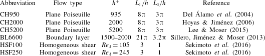
Summary of the cases most often used in the article as sources of data.
 $L_{1}$
and
 $L_{3}$
are numerical box sizes in the streamwise and spanwise direction, respectively. In all cases,
 $L_{2}=2h$
, except in the zero-pressure-gradient boundary layer BL6600, where
 $h$
is the boundary layer thickness at the middle of the box.

To save repetition in figure captions, Table 1 summarises the data sets most commonly used in the paper. For their details, the reader is directed to the original references.
When used without subindices,
 $S\equiv \unicode[STIX]{x2202}_{2}U_{1}$
is the shear of the mean velocity profile. Although shear-driven flows are generally not isotropic, we will define an ‘isotropic’ velocity fluctuation intensity,
 $q^{2}=u_{i}^{\prime }u_{i}^{\prime }$
, and an enstrophy
 ${\unicode[STIX]{x1D714}^{\prime }}^{2}=\unicode[STIX]{x1D714}_{i}^{\prime }\unicode[STIX]{x1D714}_{i}^{\prime }$
. The ‘isotropic’ dissipation rate for the fluctuating kinetic energy is
 $\unicode[STIX]{x1D700}=2\unicode[STIX]{x1D708}\unicode[STIX]{x1D634}_{ij}\unicode[STIX]{x1D634}_{ij}$
, where
 $\unicode[STIX]{x1D708}$
is the kinematic viscosity,
 $\unicode[STIX]{x1D634}_{ij}=(\unicode[STIX]{x2202}_{i}u_{j}+\unicode[STIX]{x2202}_{j}u_{i})/2$
is the fluctuating rate-of-strain tensor, and
 $\unicode[STIX]{x2202}_{j}=\unicode[STIX]{x2202}/\unicode[STIX]{x2202}x_{j}$
. Spectra of the energy or vorticity norm are defined as the sum of the spectra of the three respective components, as in
 $\unicode[STIX]{x1D719}_{qq}=\sum _{i}\unicode[STIX]{x1D719}_{u_{i}u_{i}}\equiv \unicode[STIX]{x1D719}_{ii}$
. Based on these quantities, we define the integral length scale
 $L_{\unicode[STIX]{x1D700}}=q^{3}/\langle \unicode[STIX]{x1D700}\rangle$
, the Kolmogorov viscous length
 $\unicode[STIX]{x1D702}=(\unicode[STIX]{x1D708}^{3}/\langle \unicode[STIX]{x1D700}\rangle )^{1/4}$
, and the ‘integral’ Reynolds number,
 $Re_{L}=qL_{\unicode[STIX]{x1D700}}/\unicode[STIX]{x1D708}$
. The Taylor-microscale Reynolds number is
 $Re_{\unicode[STIX]{x1D706}}=(5Re_{L}/3)^{1/2}$
.
Wall units are denoted by a ‘+’ superscript. They are defined in terms of
 $\unicode[STIX]{x1D708}$
and of the friction velocity
 $u_{\unicode[STIX]{x1D70F}}$
, which measures the total momentum transfer in the cross-shear direction and can be expressed in terms of the shear at the wall,
 $S_{w}$
, as
 $u_{\unicode[STIX]{x1D70F}}^{2}=\unicode[STIX]{x1D708}S_{w}$
. Lengths expressed in these units, such as
 $x^{+}=xu_{\unicode[STIX]{x1D70F}}/\unicode[STIX]{x1D708}$
, are Reynolds numbers, and the flow thickness
 $h^{+}$
is used as the characteristic Reynolds number of wall-bounded flows. In this normalisation,
 $\unicode[STIX]{x1D708}^{+}=1$
and can be left out of the equations. Because we will see that
 $q\sim u_{\unicode[STIX]{x1D70F}}$
, and that the largest energy-containing eddies have sizes
 $O(h)$
,
 $h^{+}$
is roughly equivalent to the integral Reynolds number
 $Re_{L}$
. Wall units, which depend on viscosity, are essentially the same as the Kolmogorov length and velocity scales, which are also based on viscosity. Although the exact correspondence depends on the flow,
 $\unicode[STIX]{x1D702}^{+}\approx 2$
at the wall, and
 $\unicode[STIX]{x1D702}^{+}\approx 0.8(x_{2}^{+})^{1/4}$
in the logarithmic range of wall distances defined in the next section (Jiménez Reference Jiménez2013b
). It is useful fact that, although not strictly equivalent,
 $\langle \unicode[STIX]{x1D700}\rangle \approx \unicode[STIX]{x1D708}{\unicode[STIX]{x1D714}^{\prime }}^{2}$
within 2 % at all wall distances, so that dissipation and enstrophy can be used interchangeably for most purposes.
3.1 Length scales and the classification into layers
The length scales of turbulence range from a small limit of the order of a few viscous Kolmogorov lengths,
 $\unicode[STIX]{x1D702}$
, to a large limit of the order of the integral length,
 $L_{\unicode[STIX]{x1D700}}$
, and it follows from the definitions in the previous section that
 $L_{\unicode[STIX]{x1D700}}/\unicode[STIX]{x1D702}=Re_{L}^{3/4}$
. This ratio is usually large, and there is an intermediate ‘inertial’ range in which neither of the two scales is important, and where eddies can only be self-similar.
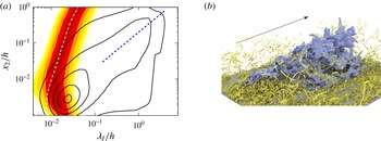
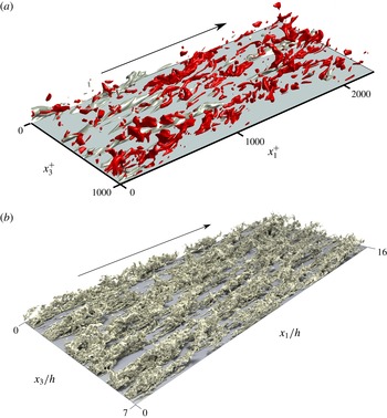
(a) The line contours are the premultiplied spectrum of the kinetic energy
 $\unicode[STIX]{x1D719}_{qq}/{u_{\unicode[STIX]{x1D70F}}}^{2}=0.5(1)4.5$
, as a function of the wall-parallel wavelength,
 $\unicode[STIX]{x1D706}_{I}$
, and of the distance from the wall. The shaded contours are the normalised premultiplied spectrum of the vorticity magnitude
 $\unicode[STIX]{x1D708}\unicode[STIX]{x1D719}_{\unicode[STIX]{x1D714}\unicode[STIX]{x1D714}}/\unicode[STIX]{x1D700}=0.5(1)4.5$
. Channel CH5200. - - -,
 $\unicode[STIX]{x1D706}_{I}=5x_{2}$
; – ⋅ – ⋅ –,
 $\unicode[STIX]{x1D706}_{I}=25\unicode[STIX]{x1D702}$
. (b) Turbulent boundary layer BL6600 at
 $h^{+}\approx 1800$
. The large central object is an isosurface of the streamwise velocity
 $(u_{1}^{+}=2)$
. It is approximately
 $2.5h$
long, and spans most of the thickness of the layer. The smaller objects are vortices visualised as isosurfaces of the discriminant of the velocity gradient. Flow is from left to right (picture credits, J. A. Sillero).

The best-known self-similar range is the Kolmogorov (Reference Kolmogorov1941) inertial energy cascade, but more relevant to our discussion is the logarithmic layer of wall-bounded flows. For an equilibrium shear flow that is statistically homogeneous in the streamwise and spanwise directions, the conservation of streamwise momentum can be written as (Tennekes & Lumley Reference Tennekes and Lumley1972),
 $$\begin{eqnarray}0=\unicode[STIX]{x2202}_{t}U_{1}=-\unicode[STIX]{x2202}_{2}\langle u_{1}u_{2}\rangle -\unicode[STIX]{x2202}_{1}P+\unicode[STIX]{x1D708}\unicode[STIX]{x2202}_{22}U_{1}=-\unicode[STIX]{x2202}_{2}\langle u_{1}u_{2}\rangle +u_{\unicode[STIX]{x1D70F}}^{2}/h+\unicode[STIX]{x1D708}\unicode[STIX]{x2202}_{22}U_{1},\end{eqnarray}$$
where
 $P=\langle \widetilde{p}\rangle$
is the ensemble-averaged kinematic pressure. Far enough from the wall for viscosity to be unimportant,
 $x_{2}^{+}\gg 1$
, but close enough for pressure gradients and other streamwise non-uniformities to be negligible,
 $x_{2}\ll h$
, (3.1) requires that the tangential Reynolds stress satisfies
 $-\langle u_{1}u_{2}\rangle \approx u_{\unicode[STIX]{x1D70F}}^{2}(1-x_{2}/h)\approx u_{\unicode[STIX]{x1D70F}}^{2}$
. This implies that the ‘correlated’ parts of
 $u_{1}$
and
 $u_{2}$
scale with
 $u_{\unicode[STIX]{x1D70F}}$
, and suggests that the same should be true for the full intensities,
 $u_{j}^{\prime }\sim q\sim u_{\unicode[STIX]{x1D70F}}$
. In addition, neither the flow thickness nor viscosity can be relevant in this range of wall distances, and there is no length scale. The result is that structures in this intermediate region can only have a characteristic aspect ratio, but not a characteristic size, and that the size of the largest momentum- and energy-carrying eddies has to grow linearly with
 $x_{2}$
.
It follows from these considerations that the possible structures of wall-bounded flows are stratified in scale space by their size, and in position by their distance from the wall, and that the flow can be approximately classified into three layers: a viscous or buffer layer, where all eddy sizes scale in wall units; an outer layer, where the length scale of the energy and of the energy production is the flow thickness
 $h$
; and a scale-less intermediate layer in which the length scale of the energy production is proportional to
 $x_{2}$
. Everywhere, the velocity scale is
 $u_{\unicode[STIX]{x1D70F}}$
, and the dissipation length is
 $\unicode[STIX]{x1D702}$
.
Spectra of the energy and enstrophy are presented in figure 3(a) in terms of an ‘isotropic’ wall-parallel wavelength
 $$\begin{eqnarray}\unicode[STIX]{x1D706}_{I}=2\unicode[STIX]{x03C0}/k_{I},\quad \text{where }k_{I}^{2}=k_{1}^{2}+k_{3}^{2},\end{eqnarray}$$
which represents the size of the eddy, but neglects for the moment the possible anisotropies of the flow. Each horizontal section of this figure is a spectral density at a given distance from the wall and, as expected, the peak of the enstrophy spectrum is everywhere near some small multiple of the Kolmogorov scale,
 $\unicode[STIX]{x1D706}_{I}^{+}\approx 25\unicode[STIX]{x1D702}^{+}\approx 20(x_{2}^{+})^{1/4}$
. For these small scales, most of the enstrophy is concentrated near
 $k_{1}\approx k_{3}$
, so that
 $\unicode[STIX]{x1D706}_{I}\approx \unicode[STIX]{x1D706}_{3}/\sqrt{2}$
and the above relation is equivalent to
 $\unicode[STIX]{x1D706}_{1}\approx \unicode[STIX]{x1D706}_{3}\approx 35\unicode[STIX]{x1D702}$
(Jiménez Reference Jiménez2013b
). On the other hand, the scale of the energy-containing eddies grows linearly away from the wall. We will see later that
 $k_{1}\ll k_{3}$
for these eddies, so that
 $\unicode[STIX]{x1D706}_{I}\approx \unicode[STIX]{x1D706}_{3}$
.
The boundary between the intermediate and outer layers, conventionally taken to be
 $x_{2}/h\approx 0.2$
, is defined by the end of the linear growth of the size of the energy-containing eddies. The transition between the intermediate and buffer layers is defined by the level,
 $x_{2}^{+}\approx 80$
(
 $x_{2}\approx 0.015h$
in figure 3
a), at which the length scales of the energy and of the enstrophy become comparable. Below this point, viscosity is important for all eddies, including the energy-containing ones. Above it, the vortices contain very little energy, and we will see below that they do not participate in the energy production.
A flow snapshot displaying the separation between the energy and dissipation scales is figure 3(b), where a perturbation velocity isosurface is shown together with the much smaller vortices. Even at this moderate Reynolds number
 $(h^{+}=1800,\,Re_{\unicode[STIX]{x1D706}}\approx 110)$
, the range of lengths is
 $L_{\unicode[STIX]{x1D700}}/\unicode[STIX]{x1D702}\approx 150$
, and it is hard to avoid the conclusion that the two types of eddies can only interact indirectly across an intermediate range in which neither the small nor the large length scale are relevant. A more extreme example is the atmospheric surface layer, where
 $\unicode[STIX]{x1D702}\approx 30~\unicode[STIX]{x03BC}\text{m}$
, and
 $h=O(100~\text{m})$
. The two scales are then separated by a factor of
 $10^{6}$
.
It is shown in appendix A that the functional relation between two variables can often be derived from their scaling properties. For example, the power law in the Kolmogorov (Reference Kolmogorov1941) inertial energy spectrum is a consequence of the lack of both a velocity and a length scale. The intermediate layer in wall-bounded turbulence lacks a length scale but not a velocity scale, and its mean velocity profile is bound to be logarithmic (see appendix A),
 $$\begin{eqnarray}U_{1}^{+}=\unicode[STIX]{x1D705}^{-1}\log x_{2}^{+}+A,\end{eqnarray}$$
from where the layer takes its common name. The constants
 $A$
and
 $\unicode[STIX]{x1D705}$
have to be determined experimentally. The Kármán constant,
 $\unicode[STIX]{x1D705}\approx 0.4$
, reflects the dynamics of turbulence in the logarithmic layer and is approximately universal, but
 $A$
is not.
The reason for the latter is that (3.3) is only a particular self-similar solution of the equations of motion, to which other solutions tend in the range of wall distances where boundary conditions can be approximately neglected. Typically, this self-similar range only exists in some limiting case (
 $h^{+}\gg 1$
in wall-bounded turbulence), outside which (3.3) is only an approximation that requires additional adjustable parameters. For example, the assumptions leading to (3.3) do not hold near the wall, and
 $A$
substitutes for the missing no-slip boundary condition. It depends on the details of the wall and of the viscous layer, and is
 $A\approx 5$
for smooth walls. Additional boundary-condition surrogates have been proposed, such as a virtual origin for
 $x_{2}$
(Oberlack Reference Oberlack2001). They improve the agreement in experiments at moderate Reynolds numbers (Mizuno & Jiménez Reference Mizuno and Jiménez2011), but can be neglected as the Reynolds number increases. In the case of a truly asymptotic logarithmic layer, even
 $A$
becomes negligible compared to
 $\log x_{2}^{+}\gg 1$
.
3.2 The energy balance
(a) Mean velocity profile for the channel CH2000. (b) Velocity fluctuation intensities: ——,
 $u_{1}^{\prime }$
; - - - -,
 $u_{2}^{\prime }$
; – ⋅ – ⋅ –,
 $u_{3}^{\prime }$
. The dashed vertical lines are conventional upper limits for the buffer
 $(x_{2}^{+}=80)$
, and logarithmic
 $(x_{2}/h=0.2)$
layers.

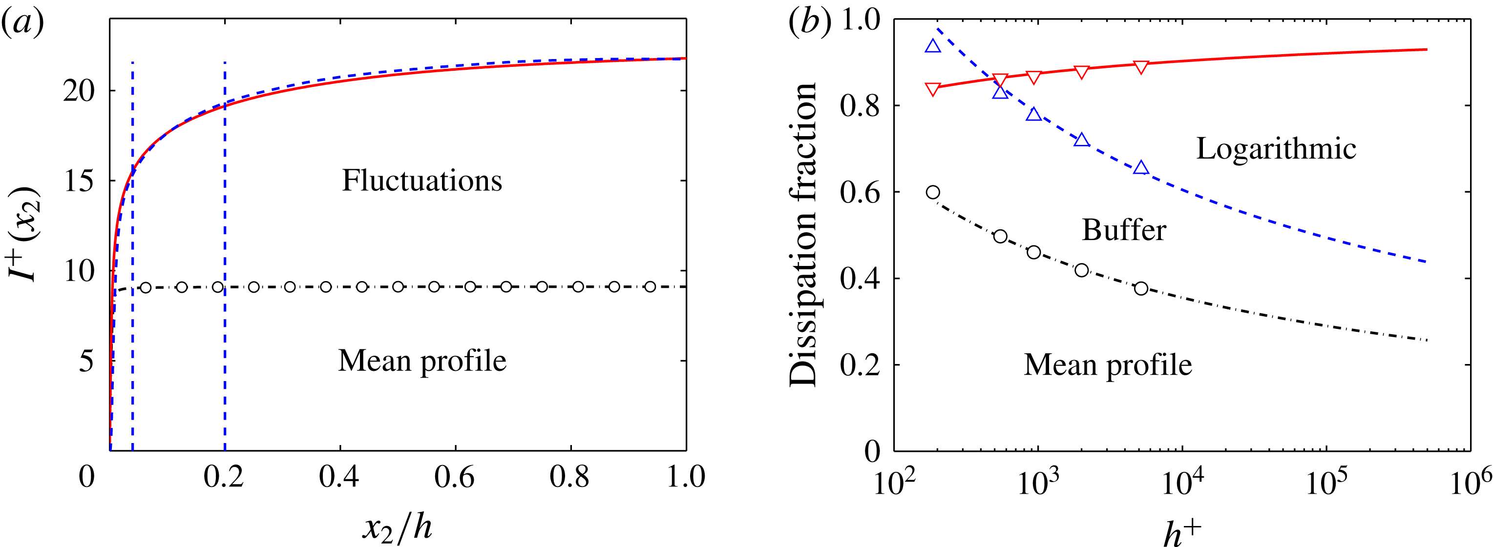
Even if they are relatively thin, the viscous and logarithmic layers are important for the flow as a whole. The thickness of the buffer layer with respect to the total thickness is
 $80/h^{+}$
, which ranges from 40 % for barely turbulent flows
 $(h^{+}\approx 200)$
to
 $10^{-4}$
for large water mains
 $(h^{+}\approx 5\times 10^{5})$
, but it follows from (3.3) that, even in the latter case, 40 % of the velocity drop takes place below
 $x_{2}^{+}=80$
(see figure 4
a). The maximum turbulence intensity is also found in the buffer layer, and the fluctuations decay away from the wall (see figure 4
b). The mean shear derived from (3.3),
 $S=u_{\unicode[STIX]{x1D70F}}/\unicode[STIX]{x1D705}x_{2}$
, which is the energy source for the turbulence fluctuations, is also maximum near the wall.
(a) Contribution to the energy dissipation below a given wall distance from the different terms in the right-hand side of (3.5). —
 $\circ$
—, Dissipation due to the mean shear; ——, total dissipation; - - - -, total energy input on the left-hand side of (3.5). The dashed vertical lines are conventional upper limits for the buffer
 $(x_{2}^{+}=80)$
, and logarithmic
 $(x_{2}/h=0.2)$
layers. Channel CH2000. (b) Fraction of the dissipation due to different layers in channels, versus the Reynolds number.
 $\circ$
, from the mean shear; ▵, below
 $x_{2}^{+}=80$
; ▿, below
 $x_{2}/h=0.2$
. The trend lines are the semiempirical fits discussed in the text: – ⋅ – ⋅ –,
 $9.1/U_{b}^{+}$
; - - - -,
 $15.5/U_{b}^{+}$
; ——,
 $1-2.5/U_{b}^{+}$
.

Consider the energy balance in a turbulent channel (Tennekes & Lumley Reference Tennekes and Lumley1972). Energy enters the system through the work of the pressure gradient
 $\unicode[STIX]{x2202}_{1}P=-u_{\unicode[STIX]{x1D70F}}^{2}/h$
on the volumetric flux
 $2hU_{b}$
, where
 $U_{b}=h^{-1}\int _{0}^{h}U_{1}\,\text{d}x_{2}$
is the bulk velocity. This energy input has to balance the total dissipation if the flow is to be statistically stationary. In wall units, this is expressed as
 $$\begin{eqnarray}h^{+}U_{b}^{+}=\int _{0}^{h^{+}}U_{1}^{+}\,\text{d}x_{2}^{+}=\int _{0}^{h^{+}}(\unicode[STIX]{x1D700}^{+}+{S^{+}}^{2})\,\text{d}x_{2}^{+},\end{eqnarray}$$
where
 $\unicode[STIX]{x1D700}$
in the last integral is the ‘turbulent’ dissipation due to the gradients of the velocity fluctuations, and
 ${S^{+}}^{2}$
is the dissipation due to the effect of the viscosity on the mean velocity profile. When the balance leading to (3.4) is applied to a layer stretching from the wall to
 $x_{2}$
it gives an idea of the contributions to the dissipation from the different parts of the flow. The equation takes the form,
 $$\begin{eqnarray}I^{+}(x_{2})=-\langle u_{1}u_{2}\rangle ^{+}U_{1}^{+}+\int _{0}^{x_{2}^{+}}U_{1}^{+}\,\text{d}\unicode[STIX]{x1D709}=\int _{0}^{x_{2}^{+}}(\unicode[STIX]{x1D700}^{+}+{S^{+}}^{2})\,\text{d}\unicode[STIX]{x1D709}+\cdots \,,\end{eqnarray}$$
where the extra term in the energy input in the left-hand side is the work of the tangential Reynolds stress against the mean profile. The two terms in the right-hand side of (3.5) are plotted in figure 5(a). The small difference between the energy input (dashed) and the dissipation (solid line) in this figure is the effect of the small internal energy fluxes represented by the trailing dots in (3.5). They are negligible at high Reynolds numbers.
In shear flows without walls, the dissipation due to the mean velocity profile is
 $O(\unicode[STIX]{x1D700}/Re)$
, and can be neglected. In the wall-bounded case, figure 5(a) shows that both contributions are of the same order, although the dissipation due to the mean profile resides almost exclusively below
 $x_{2}^{+}=20$
. Because the shear in that region scales well in wall units, this part of the dissipation is very nearly independent of the Reynolds number,
 $\int _{0}^{h}{S^{+}}^{2}\,\text{d}x_{2}\approx 9.1$
. Figure 5(a) also shows that a relatively large fraction of the turbulent dissipation, denoted as
 $\unicode[STIX]{x1D700}_{80}$
, takes place below
 $x_{2}^{+}=80$
. The velocity gradients in this part of the flow are also approximately independent of the Reynolds number, and
 $\unicode[STIX]{x1D700}_{80}^{+}\approx 6.4$
.
Most of the remaining dissipation takes place within the logarithmic layer,
 $80\unicode[STIX]{x1D708}/u_{\unicode[STIX]{x1D70F}}<x_{2}<0.2h$
, and can be estimated from (3.3). The energy balance of the fluctuations, averaged over wall-parallel planes, takes the form (Tennekes & Lumley Reference Tennekes and Lumley1972)
 $$\begin{eqnarray}0=\text{D}_{t}\langle q^{2}/2\rangle =-S\langle u_{1}u_{2}\rangle -\langle \unicode[STIX]{x1D700}\rangle +\cdots \,,\end{eqnarray}$$
where
 $\text{D}_{t}=\unicode[STIX]{x2202}_{t}+U_{1}\unicode[STIX]{x2202}_{1}$
is the mean advective derivative. The trailing dots stand for transfer terms that are not important in the logarithmic layer, where the dissipation is almost exclusively due to
 $\unicode[STIX]{x1D700}$
, and has to be approximately balanced by the local energy production,
 $-S\langle u_{1}u_{2}\rangle$
. This can be written as
 $$\begin{eqnarray}\unicode[STIX]{x1D700}^{+}\approx -\langle u_{1}u_{2}\rangle ^{+}S^{+}\approx (1-x_{2}/h)/\unicode[STIX]{x1D705}x_{2}^{+},\end{eqnarray}$$
which can be integrated to
 $$\begin{eqnarray}\unicode[STIX]{x1D700}_{log}^{+}\approx \int _{80}^{0.2h^{+}}\unicode[STIX]{x1D700}^{+}\,\text{d}x_{2}^{+}\approx \unicode[STIX]{x1D705}^{-1}\log h^{+}-15.5.\end{eqnarray}$$
A similar estimate for the total energy input shows that
 $$\begin{eqnarray}U_{b}^{+}\approx \unicode[STIX]{x1D705}^{-1}\log h^{+}+2.5\end{eqnarray}$$
also grows logarithmically with
 $h^{+}$
, so that the remaining dissipation above the logarithmic layer is approximately independent of the Reynolds number,
 $\unicode[STIX]{x1D700}_{out}^{+}\approx 2.5$
. As a consequence, the relative contributions of the buffer and outer layers to the dissipation decrease logarithmically as the Reynolds number increases. This is shown in figure 5(b), which includes simulation results from channels at several Reynolds numbers, and logarithmic fits based on the arguments above. In the asymptotic limit of an ‘infinite’ Reynolds number, most of the dissipation resides in the logarithmic layer, but figure 5(b) shows that the fraction of the dissipation due to the mean and fluctuating velocities in the buffer layer is still of the order of 50 % of the total at the largest ‘realistic’ Reynolds numbers,
 $h^{+}=O(10^{6})$
.
Because of this ‘singular’ nature, the near-wall layer is not only important for the rest of the flow, but it is also essentially independent from it. This was shown by Jiménez & Pinelli (Reference Jiménez and Pinelli1999) using ‘autonomous’ simulations in which the outer flow was artificially removed above a certain distance,
 $\unicode[STIX]{x1D6FF}$
, from the wall. The dynamics of the buffer layer was unaffected as long as
 $\unicode[STIX]{x1D6FF}^{+}\gtrsim 60$
. The same conclusion can be drawn from the minimal flow experiments by Jiménez & Moin (Reference Jiménez and Moin1991), who simulated channels in numerical boxes small enough for no large flow scales to be possible above
 $x_{2}^{+}\approx 100$
. Again, the buffer layer remained essentially unaffected. Minimal flows were extended to the logarithmic layer by Flores & Jiménez (Reference Flores and Jiménez2010) with similar results: the dynamics of the higher-shear region near the wall is essentially independent from outside influences. These observations should not be interpreted to mean that there are no interactions between the inner and outer layers. These interactions will be documented below, but they can mostly be expressed as modulations or superpositions, which are not required for the maintenance of the flow.
Understanding the structure of this near-wall region has practical implications. Energy dissipation by turbulence is the root cause of hydrodynamic friction drag, which is estimated to be responsible for 5 % of the total energy expenditure of humankind (Jiménez Reference Jiménez2013b
). The energy input,
 $U_{b}^{+}=(2/c_{f})^{1/2}$
, determines the friction coefficient
 $c_{f}$
, and it follows from figure 5 that any attempt to understand or to control wall friction has to take into account the buffer and logarithmic layers.
3.3 The scales of the energy production
The above discussion says little about how turbulence extracts energy from the mean flow. We saw in (3.6) that the average energy production in a parallel shear flow is
 $-S\langle u_{1}u_{2}\rangle$
, which depends on the coupling of the Reynolds stress with the mean shear.
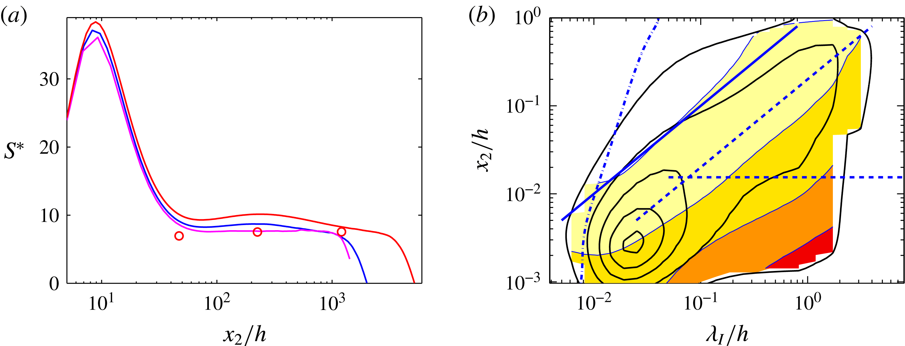
(a) Corrsin (Reference Corrsin1958) integral shear parameter
 $S^{\ast }$
. ——, Channels and boundary layers
 $h^{+}=2000{-}5200$
(various sources);
 $\circ$
, statistically stationary homogeneous shear turbulence, plotted at the equivalent
 $Re_{\unicode[STIX]{x1D706}}$
(Sekimoto et al.
Reference Sekimoto, Dong and Jiménez2016). (b) The line contours are the spectral energy density of the kinetic energy, as in figure 3(a). The shaded contours are the spectral Corrsin shear parameter
 $s^{\ast }(\unicode[STIX]{x1D706}_{I})=2(\times 10)2000$
, from light to dark. Channel CH5200. ——,
 $\unicode[STIX]{x1D706}_{I}=x_{2}$
; - - - -,
 $\unicode[STIX]{x1D706}_{I}=5x_{2}$
; – ⋅ – ⋅ –,
 $\unicode[STIX]{x1D706}_{I}=25\unicode[STIX]{x1D702}$
. The horizontal dashed line is
 $x_{2}^{+}=80$
.

The coupling criterion was established by Corrsin (Reference Corrsin1958). The turnover time over which the nonlinear self-interaction of an eddy of size
 $\ell$
and characteristic velocity
 $u_{\ell }$
changes its energy is of order
 $\unicode[STIX]{x1D70F}_{to}=\ell /u_{\ell }$
, while its deformation by the shear takes place in
 $\unicode[STIX]{x1D70F}_{s}=S^{-1}$
. The Corrsin parameter is the ratio of these times,
 $s^{\ast }(\ell )=\unicode[STIX]{x1D70F}_{to}/\unicode[STIX]{x1D70F}_{s}=S\ell /u_{\ell }$
. If
 $s^{\ast }(\ell )\ll 1$
, the eddy evolves independently of the shear and there is little or no energy production. This is the regime of the inertial cascade. If
 $s^{\ast }(\ell )\gg 1$
, the eddy is controlled by the shear, and can extract (or lose) energy from (or to) it. This is the range of the energy production. Note that this implies that the energy-producing eddies of a shear flow are quasilinear, in the sense that they are controlled by the interaction of the fluctuations with the mean flow, with only slower nonlinear effects. The inertial cascade is fully nonlinear.
When this criterion is applied to the integral scales, where
 $\ell =L_{\unicode[STIX]{x1D700}}$
and
 $u_{\ell }=q$
, we obtain an integral Corrsin parameter,
 $S^{\ast }=Sq^{2}/\unicode[STIX]{x1D700}$
, which determines whether some part of the flow is involved in the production of turbulent energy (if
 $S^{\ast }\gg 1$
), or just transfers or dissipates it (if
 $S^{\ast }\ll 1$
).
Figure 6(a) shows that equilibrium shear flows tend to have
 $S^{\ast }\approx 10$
, at least above the buffer layer in the wall-bounded case. This is a moderately large number that implies a quasilinear interaction of the energy-containing eddies with the mean flow throughout the whole logarithmic layer. Linear processes do not have an intrinsic amplitude, and the fact that
 $S^{\ast }$
is similar for fairly different flows suggests that the ‘linear’ energy production eventually saturates by means of a relatively universal mechanism that drains its energy to the cascade, roughly equivalent to an eddy viscosity (del Álamo & Jiménez Reference del Álamo and Jiménez2006). This recalls the engineering rule of thumb that the Reynolds number based on the eddy viscosity of turbulent flows is always of order 10–30 (Tennekes & Lumley Reference Tennekes and Lumley1972). The very high value of
 $S^{\ast }$
in the buffer layer is not an indicator of extremely sheared flow in the sense just discussed. The shear in this region is the highest in the flow, but the argument of Corrsin (Reference Corrsin1958) assumes that the balance is between nonlinearity and shear, while the fastest evolution time near the wall is viscous. For eddies of size
 $\ell$
the viscous decay time is
 $T_{\unicode[STIX]{x1D708}}=\ell ^{2}/\unicode[STIX]{x1D708}$
, and the relevant shear parameter is
 $S_{\unicode[STIX]{x1D708}}^{\ast }=S\ell ^{2}/\unicode[STIX]{x1D708}$
. In fact, the transition of
 $S^{\ast }$
from its near-wall peak to the outer plateau can be used as a convenient definition of the upper edge of the buffer layer, and is the origin of the value used in this article,
 $x_{2}^{+}\approx 80$
.
The spectral shear parameter for individual wavelengths,
 $s^{\ast }(\unicode[STIX]{x1D706}_{I},x_{2})$
, can be estimated by identifying the eddy size
 $\ell$
with the wavelength
 $\unicode[STIX]{x1D706}_{I}$
, and the eddy velocity scale with the spectral energy density
 $u_{\ell }=\unicode[STIX]{x1D719}_{qq}^{1/2}$
. The resulting
 $s^{\ast }=S\unicode[STIX]{x1D706}_{I}/\unicode[STIX]{x1D719}_{qq}^{1/2}$
is overlaid in figure 6(b) to the energy spectrum from figure 3(a). It increases sharply towards the longer wavelengths near the wall, and falls below
 $s^{\ast }=2$
to the left of
 $\unicode[STIX]{x1D706}_{I}\approx L_{c}=x_{2}$
. The Corrsin length
 $L_{c}$
defined in this way represents the scale of the smallest eddies that interact directly with the shear, and is typically a fixed small fraction of the integral length,
 $L_{c}/L_{\unicode[STIX]{x1D700}}\approx (S^{\ast })^{-3/2}$
. As in figure 6(a), the shear-dominated region below
 $x_{2}^{+}\approx 80$
should be interpreted as viscous, including the highest
 $s^{\ast }$
in the very long near-wall region in the lower right-hand corner of figure 6(b).
Note that, as expected, the length scale of the vorticity,
 $\unicode[STIX]{x1D706}_{I}\approx 25\unicode[STIX]{x1D702}$
, is below the Corrsin scale for
 $x_{2}^{+}\gtrsim 50$
, equivalent to
 $x_{2}/h\approx 10^{-2}$
in the case of figure 6(b). Except in the buffer layer, these viscous vortices do not interact with the shear, and do not participate in the turbulence-production process.
3.4 Anisotropy
Although figure 3(a) is drawn in terms of an isotropic wavelength and of the kinetic energy, shear flows are not isotropic. Figure 4(b) shows that the intensities of the three velocity components are different. The largest share of the kinetic energy is contained in
 $u_{1}^{\prime 2}$
. This is especially true in the buffer layer, but the contribution of this component is at least half of the total at all wall distances. The other two velocity components split the rest of the energy approximately evenly, at least far from the wall. This is most easily understood in terms of the energy equation for individual components (Tennekes & Lumley Reference Tennekes and Lumley1972), although we will see later how this difference is implemented in detail by the energy-production mechanisms. In a channel,
 $$\begin{eqnarray}0=\text{D}_{t}\langle u_{1}^{2}/2\rangle =-S\langle u_{1}u_{2}\rangle +\langle p\,\unicode[STIX]{x2202}_{1}u_{1}\rangle -\unicode[STIX]{x1D708}\langle |\unicode[STIX]{x1D735}u_{1}|^{2}\rangle +\cdots \,,\end{eqnarray}$$
for the streamwise component, and
 $$\begin{eqnarray}0=\text{D}_{t}\langle u_{m}^{2}/2\rangle =\langle p\,\unicode[STIX]{x2202}_{m}u_{m}\rangle -\unicode[STIX]{x1D708}\langle |\unicode[STIX]{x1D735}u_{m}|^{2}\rangle +\cdots \,,\quad m=2,3,\end{eqnarray}$$
for each of the two transverse components, where the repeated indices in the pressure term do not imply summation. The streamwise component is special because, on average, it is the only one that receives energy directly from the shear through the production term,
 $-S\langle u_{1}u_{2}\rangle$
. Approximately half of this energy is dissipated to viscosity, and the rest is transferred to the other two velocity components by the pressure–strain term,
 $\langle p\,\unicode[STIX]{x2202}_{1}u_{1}\rangle$
. This is a redistribution term, because it follows from continuity that
 $\langle p\,\unicode[STIX]{x2202}_{j}u_{j}\rangle =0$
, so that the net effect of the pressure on the kinetic energy vanishes. Its effect on the velocities is approximately isotropic, and each of the two transverse components receives roughly equal amounts of energy (Hoyas & Jiménez Reference Hoyas and Jiménez2008). Roughly speaking, the kinetic energy of the streamwise velocity is twice that of the other two components because it receives twice as much energy as they do.
The details of the distribution of the kinetic energy among the three velocity components depend on the flow. The buffer layer is approximately universal, but the outer layers are not. The contribution of the transverse velocities to the kinetic energy is somewhat larger in boundary layers than in channels, most probably due to the intermittency at the turbulent–non-turbulent interface (Sillero et al. Reference Sillero, Jiménez and Moser2013). In contrast, the streamwise component is substantially stronger in Couette flow than in either boundary layers or channels, reflecting the presence of strong persistent streamwise ‘rollers’ which are not found in other flows (Pirozzoli, Bernardini & Orlandi Reference Pirozzoli, Bernardini and Orlandi2014).
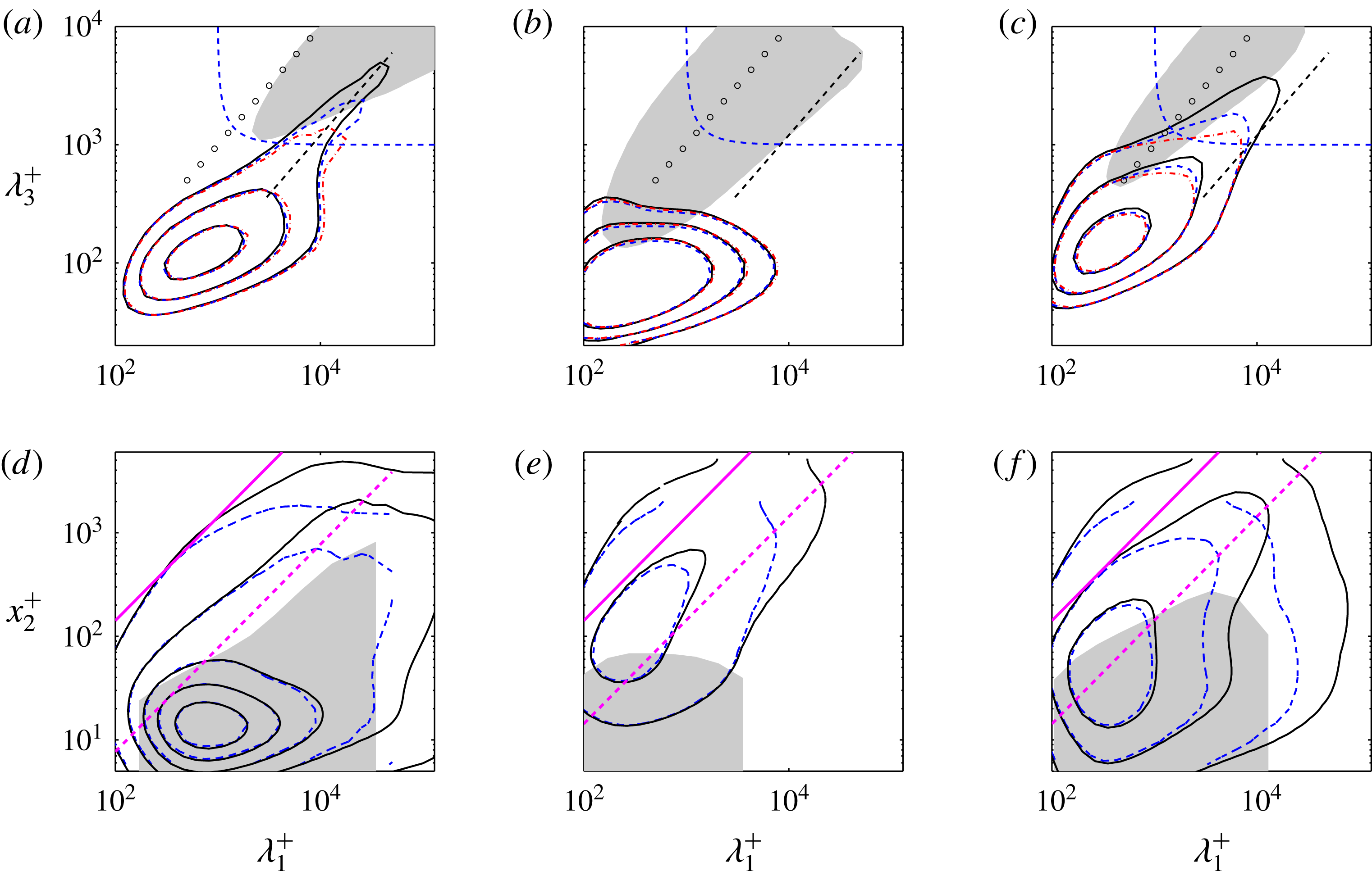
(a–c) Two-dimensional spectral densities of the velocity components at
 $x_{2}^{+}=15$
. The dashed diagonal is
 $\unicode[STIX]{x1D706}_{1}=8\unicode[STIX]{x1D706}_{3}$
, the hyperbolic curve is
 $\unicode[STIX]{x1D706}_{I}^{+}=1000$
, and the circles are
 $\unicode[STIX]{x1D706}_{1}=\unicode[STIX]{x1D706}_{3}$
. The grey patch is the integrated energy density,
 $\unicode[STIX]{x1D6F7}=(1/h)\int _{0}^{h}\unicode[STIX]{x1D719}\,\text{d}x_{2}$
for
 $h^{+}=5200$
. (a)
 $\unicode[STIX]{x1D719}_{11}^{+}=(0.25,0.5,1.0)$
.
 $\unicode[STIX]{x1D6F7}_{11}^{+}=0.1$
(b)
 $\unicode[STIX]{x1D719}_{22}^{+}=(0.006,0.012,0.025)$
.
 $\unicode[STIX]{x1D6F7}_{22}^{+}=0.02$
(c)
 $\unicode[STIX]{x1D719}_{33}^{+}=(0.05,0.1,0.2)$
.
 $\unicode[STIX]{x1D6F7}_{33}^{+}=0.05$
(d–f). One-dimensional streamwise spectral densities as functions of wall distance. The two diagonals are approximately: ——,
 $\unicode[STIX]{x1D706}_{I}=x_{2}$
; - - - -,
 $\unicode[STIX]{x1D706}_{I}=5x_{2}$
, converted to
 $\unicode[STIX]{x1D706}_{1}$
by taking into account the aspect ratio of the outer-layer spectra. (d)
 $\unicode[STIX]{x1D719}_{11}^{+}=0.2(0.4)1.8$
. The grey patch is the vertically correlated region near the wall for
 $h^{+}=2003$
, from figure 11(e). (e) As in (d), for
 $\unicode[STIX]{x1D719}_{22}^{+}=0.1(0.2)0.9$
. (f)
 $\unicode[STIX]{x1D719}_{33}^{+}=0.1(0.2)0.9$
. Channels: – ⋅ – ⋅ –, CH950; - - - -, CH2000; ——, CH5200.

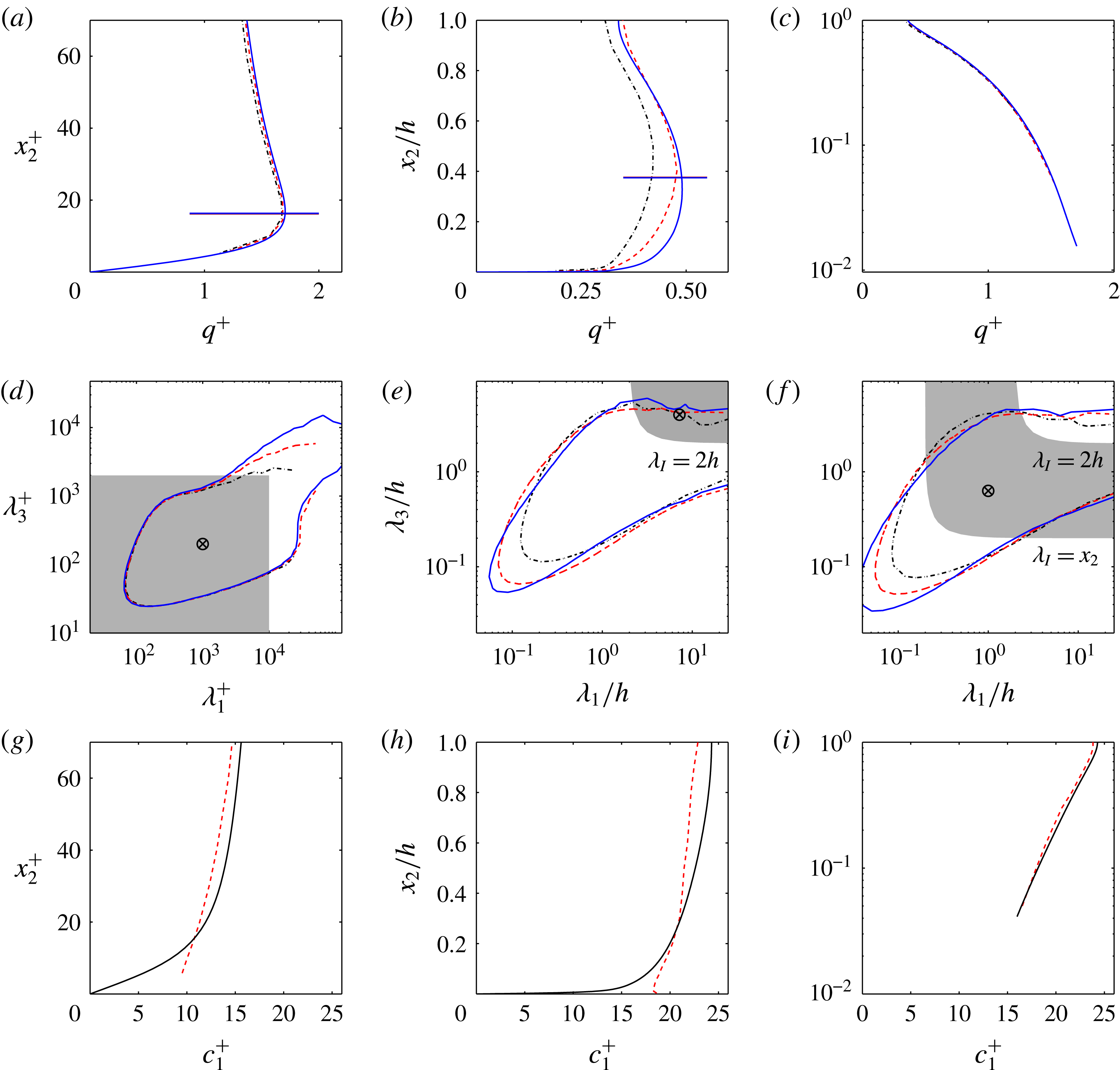
Figures 7(a)–7(c) display wall-parallel two-dimensional spectral densities for the three velocity components at the location of the buffer-layer peak of
 $u_{1}^{\prime }$
. The streamwise-velocity spectrum in figure 7(a) has two well differentiated parts (Hoyas & Jiménez Reference Hoyas and Jiménez2006): a near-wall one for
 $\unicode[STIX]{x1D706}_{I}^{+}\lesssim 10^{3}$
, which scales in wall units; and a ridge along
 $\unicode[STIX]{x1D706}_{1}\approx 8\unicode[STIX]{x1D706}_{3}$
, which gets longer as
 $h^{+}$
increases, and is therefore associated with the outer flow. Figures 7(a)–7(c) also contain an isocontour of the vertically integrated energy densities,
 $\unicode[STIX]{x1D6F7}=(1/h)\int _{0}^{h}\unicode[STIX]{x1D719}\,\text{d}x_{2}$
, showing that the large-scale energy in the buffer region is generally only associated with the long-wavelength edge of the integrated spectrum. Most of the kinetic energy, which resides in the outer part of the flow, does not reach near the wall.
The wall-normal structure of these spectra is displayed in figure 7(d–f) as spanwise-integrated one-dimensional spectral densities, plotted as functions of the distance from the wall and of the streamwise wavelength. The first conclusion from figure 7 is that the wall-normal velocity is damped in the neighbourhood of the wall, and that the damping is strongest for the largest eddies. There is no large-scale
 $\unicode[STIX]{x1D719}_{22}$
in figure 7(b), even if the contours in this figure are forty times weaker than those for
 $\unicode[STIX]{x1D719}_{11}$
in figure 7(a). Farther from the wall, the transverse velocities in figures 7(e) and 7(f) are weaker than
 $u_{1}$
, but only by a factor of two, which is also the ratio of their overall intensities. Moreover, the comparison of the different spectra, using as reference the various trend lines in the figures, shows that
 $u_{2}$
and
 $u_{3}$
tend to occur at similar scales far from the wall, suggesting that they may be part of a common structure in that region, while
 $u_{1}$
and
 $u_{3}$
are similarly paired near it. This is also suggested by the shaded grey patches in figure 7(d–f), which mark the depth of the near-wall vertically coherent layer for the three velocities. This information cannot be obtained from the spectra, and will be discussed in detail in § 3.5, but the results have been added to figure 7(d–f) to aid in their interpretation. There is a near-wall layer in which all the velocity components are vertically correlated, but the coherent layer of
 $u_{2}$
does not extend beyond
 $\unicode[STIX]{x1D706}_{1}^{+}\approx 5000$
and
 $x_{2}^{+}\approx 80$
, scaling in wall units. The coherent layer of
 $u_{1}$
and
 $u_{3}$
extends up to
 $\unicode[STIX]{x1D706}_{1}\approx 7h$
and
 $x_{2}/h\approx 0.1{-}0.2$
, scaling in outer units. Beyond
 $\unicode[STIX]{x1D706}_{1}\approx 7h$
, the near-wall coherent layer of
 $u_{3}$
disappears, but
 $u_{1}$
continues to get taller until it fills most of the channel at very long wavelengths.
The grey patches in figure 7(a–c) show that the spectra of the three velocities are very different above the buffer layer. The two transverse components are approximately equilateral,
 $\unicode[STIX]{x1D706}_{1}\approx \unicode[STIX]{x1D706}_{3}$
, but the spectrum of the streamwise velocity is longer. Its short-wavelength edge,
 $\unicode[STIX]{x1D706}_{1}\approx 2\unicode[STIX]{x1D706}_{3}$
, is only slightly more elongated than for the transverse velocities, but its longest wavelengths are at least ten times longer than for the two transverse velocities, and extend to the longest dimension of the computational box. This long-wavelength behaviour will be discussed in the next section, and suggests that, if there are coherent structures in the flow, there are at least two kinds: very elongated ‘streaks’ of
 $u_{1}$
, and shorter structures of
 $(u_{2},u_{3})$
.
3.5 Correlations
While spectra describe the size of eddies along homogeneous directions, non-homogeneous directions have to be analysed using two-point covariances, defined for
 $u_{i}$
as
 $$\begin{eqnarray}R_{ii}(\boldsymbol{x},\tilde{\boldsymbol{x}})=\langle u_{i}(\boldsymbol{x})u_{i}(\tilde{\boldsymbol{x}})\rangle ,\end{eqnarray}$$
where the repeated index does not imply summation. The covariance is symmetric in its two arguments, but we will define
 $\tilde{\boldsymbol{x}}$
as the reference point, and
 $\boldsymbol{x}$
as the variable argument. Along homogeneous directions,
 $R_{ii}$
depends only on the coordinate increment,
 $\unicode[STIX]{x0394}x_{j}=x_{j}-\tilde{x}_{j}$
, and forms a Fourier-transform pair with the power spectrum (see appendix B.2). For example, in channels,
 $R_{ii}=R_{ii}(\unicode[STIX]{x0394}x_{1},x_{2},\tilde{x}_{2},\unicode[STIX]{x0394}x_{3})$
. At the reference point, the covariance reduces to the variance
 $R_{ii}(\tilde{\boldsymbol{x}},\tilde{\boldsymbol{x}})=u_{i}^{\prime 2}(\tilde{\boldsymbol{x}})$
, and the dimensionless version of the covariance is the two-point correlation,
 $$\begin{eqnarray}C_{ii}(\boldsymbol{x},\tilde{\boldsymbol{x}})=\frac{\langle u_{i}(\boldsymbol{x})u_{i}(\tilde{\boldsymbol{x}})\rangle }{u_{i}^{\prime }(\boldsymbol{x})u_{i}^{\prime }(\tilde{\boldsymbol{x}})},\end{eqnarray}$$
which is unity at
 $\boldsymbol{x}=\tilde{\boldsymbol{x}}$
. Correlations and covariances are high-dimensional quantities. In channels, the correlation is four-dimensional. In boundary layers, where the only homogeneous direction is the span, it is five-dimensional. This means that, except for relatively low Reynolds numbers, it is difficult to compute and store correlations or covariances for more than a few reference points. For a channel simulation using a moderately sized grid with
 $m=1000^{3}=10^{9}$
points, the correlation is an
 $(m\times m)$
matrix, which can be reduced, using homogeneity, to a block-diagonal form of
 $m^{2/3}=10^{6}$
submatrices of size
 $(m^{1/3}\times m^{1/3})$
. The total number of non-zero elements is
 $m^{4/3}=10^{12}$
, although the rank is only
 $m$
. The problem of using empirical correlations is more fundamental than a practical question of computer storage. It is shown in appendix B that the covariance can be represented as a matrix
 $\unicode[STIX]{x1D64D}=\unicode[STIX]{x1D650}\unicode[STIX]{x1D650}^{\ast }$
, where
 $\unicode[STIX]{x1D650}$
is an
 $(m\times n)$
matrix whose columns are the
 $n$
observations (‘snapshots’), and the asterisk denotes Hermitian transpose. It is clear from this definition that the rank of
 $\unicode[STIX]{x1D64D}$
constructed in this way is at most
 $n$
. The consequence is that the computation of the covariance requires as many independent snapshots as degrees of freedom, which increases with the cube of the grid diameter. Any smaller number of independent samples only provides an approximation to the covariance. In practice, this means that covariances are typically only used in the form of incomplete approximations of deficient rank, usually through some variant of the method of snapshots (Sirovich Reference Sirovich1987, see appendix B.1).
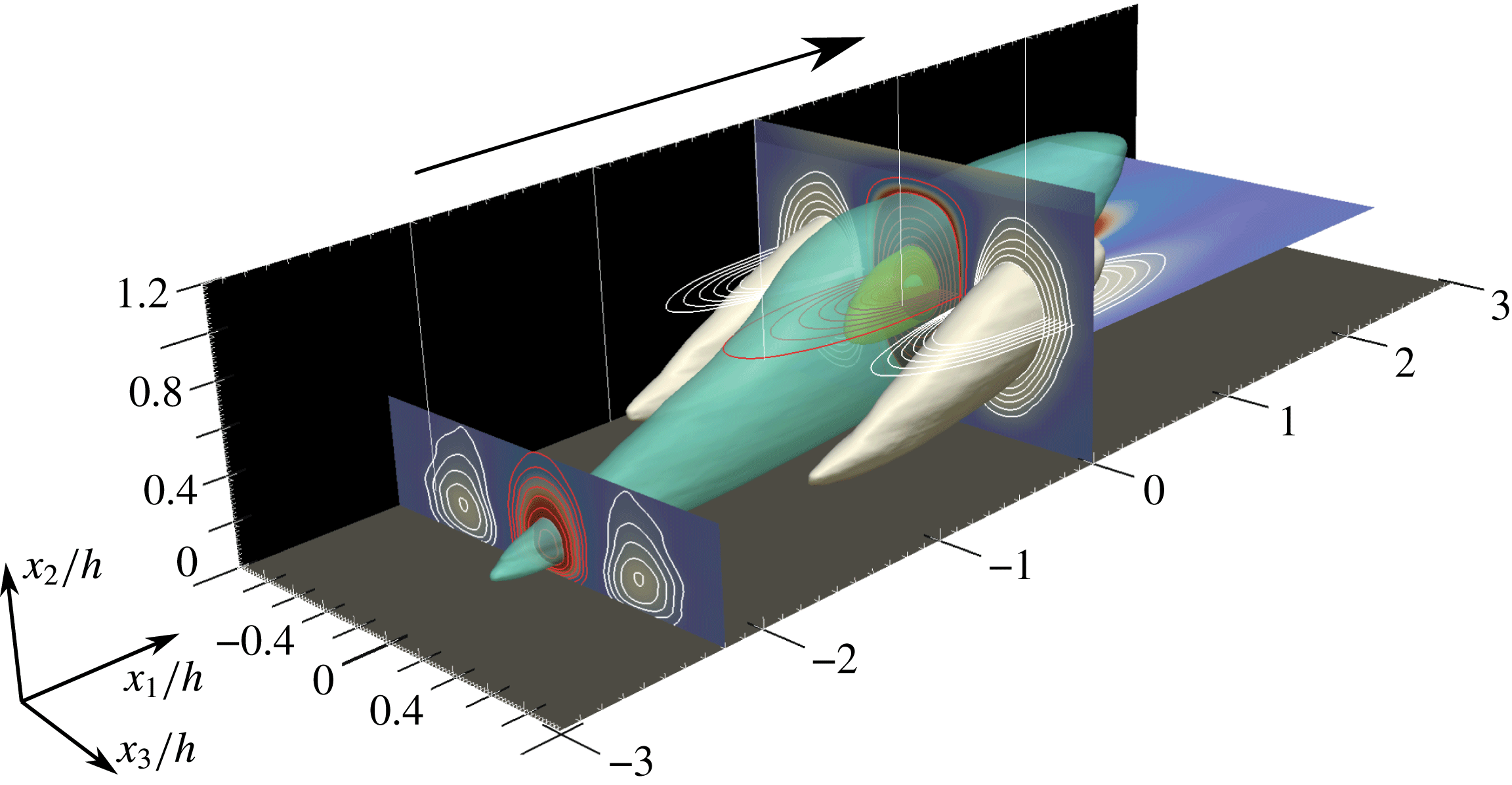
Three-dimensional representation of the correlation function of the streamwise-velocity fluctuations,
 $C_{11}$
, with respect to the reference point
 $\tilde{x}_{2}/h=0.6$
. Boundary layer BL6600 at
 $h^{+}=1530$
. The flow goes from left to right. Several isosurfaces are shown, with
 $C_{11}=-0.09$
(white),
 $+0.09$
(turquoise),
 $+0.4$
(yellow) and
 $+0.8$
(blue). In the different planar cross-sections, the contour lines of positive and negative values are coloured red and white, respectively. Reproduced with permission from Sillero, Jiménez & Moser (Reference Sillero, Jiménez and Moser2014).

In spite of these limitations, correlations give useful information about the three-dimensional structure of the flow variables. Figure 8 is an example of
 $C_{11}$
for a boundary layer. It shows an inclined central positive lobe surrounded by smaller negative lobes. The cross-flow sections are approximately circular, while the streamwise sections are elongated. Most of the data in this subsection are drawn from Sillero et al. (Reference Sillero, Jiménez and Moser2014), which should be consulted for further details. As in spectra, it is striking that the correlations of the different velocity components have very different geometries. While the inclination angle of the streamwise-velocity correlation in figure 8 is approximately
 $10^{\circ }$
with respect to the wall, the correlation of the wall-normal velocity is vertical, and that of the spanwise velocity is tilted approximately
 $30^{\circ }$
. These values remain approximately constant away from the buffer and outer layers, apply to boundary layers and channels, and are independent of the Reynolds number within the range in which they have been studied. The correlation of the pressure fluctuations is also vertical, broadly similar to that of
 $u_{2}$
.
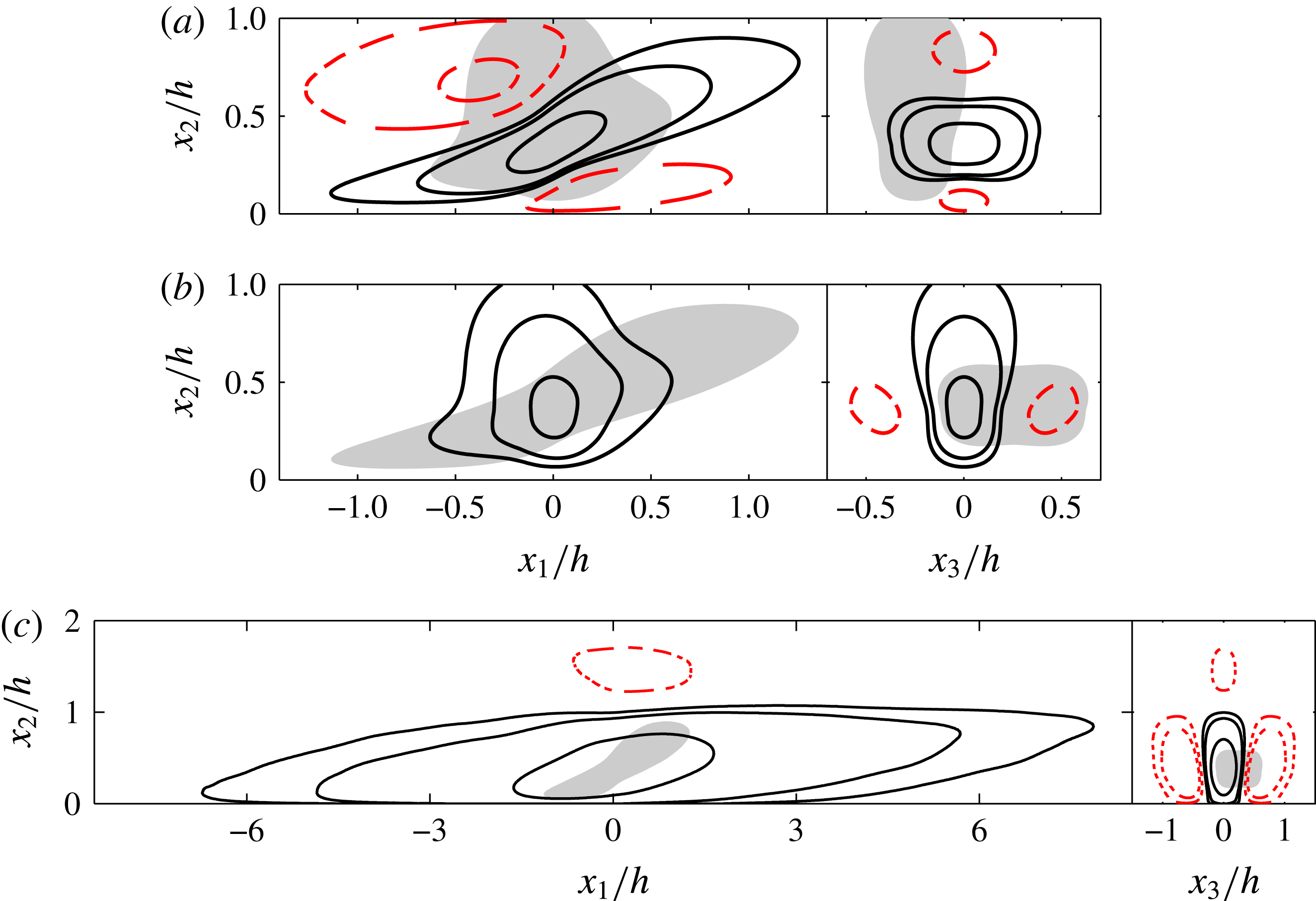
Two-dimensional sections through the reference point
 $(\tilde{x}_{2}/h=0.35)$
of the two-point autocorrelation function of the three velocity components. Channel CH2000. (a) Spanwise velocity. (b) Wall-normal velocity. (c) Streamwise velocity. Contours are
 $C=[-0.1,-0.05,0.05,0.1,0.3]$
. Negative contours are dashed. The grey patches in (a–b) are the
 $C=0.05$
contour of the other transverse-velocity component. It has been shifted horizontally by
 $0.25h$
in the cross-flow sections to suggest a possible completion of the streamwise roller. The grey patch in (c) is
 $C_{33}$
.

Streamwise and cross-flow sections of the velocity autocorrelation function of the three velocity components are given in figure 9 for a reference point in the outer edge of the logarithmic region,
 $\tilde{x}_{2}/h=0.35$
. This is approximately where the correlations of
 $u_{1}$
are longest in channels. The correlations of the two transverse velocities in figure 9(a,b) have comparable dimensions. As mentioned above, the correlation of the spanwise velocity in figure 9(a) is tilted at approximately 30
 $^{\circ }$
to the wall. It has relatively strong negative lobes which are tilted at approximately the same inclination, located above and below the main positive lobe. The cross-flow section in the right-hand part of figure 9(a) shows that the positive correlation lobe is flat and wide with respect to its height. Conversely, the correlation of the wall-normal velocity in figure 9(b) is relatively isotropic in the streamwise section, slightly tilted backwards, and tall and narrow in the cross-flow plane.
It should be noted that the centres of the two correlations do not necessarily correspond to the same location in the homogeneous wall-parallel directions. Correlations describe the relation between the same velocity component at two points. For example, a positive
 $C_{22}$
means that
 $u_{2}(x_{2})$
has, on average, the same sign as
 $u_{2}(\tilde{x}_{2})$
, but their common sign can be positive or negative. Similarly,
 $C_{22}$
and
 $C_{33}$
say little about the relative position of
 $u_{2}$
with respect to
 $u_{3}$
. However, if figures 9(a) and 9(b) are taken together, they are consistent with a ‘roller’, oriented approximately streamwise and inclined at 30
 $^{\circ }$
to the wall. The positive lobe of
 $C_{33}$
would correspond to the top or to the bottom of the roller, where the transverse velocity is directed spanwise. Its negative lobe corresponds to the other edge of the roller, where
 $u_{3}$
has opposite sign. The positive lobe of
 $C_{22}$
would correspond to the two ‘sidewalls’ closing the circuit. Grey patches of
 $C_{22}$
have been added to the
 $C_{33}$
plot, and vice versa, to suggest the relation implied by this model between the two components. The two correlations have been shifted by
 $0.25h$
in the spanwise direction, to make
 $C_{22}$
coincide with a possible lateral edge of the roller. This offset would imply a roller diameter of approximately
 $0.5h$
, of the same order as the distance from the wall to the reference point,
 $\tilde{x}_{2}=0.35h$
, and consistent with the vertical distance between the positive and negative lobes of
 $C_{33}$
. The negative lobes in the transverse cross-section of
 $C_{22}$
in figure 9(b) are also at the right distance and position to represent the opposite lateral wall of the roller. Note that the symmetry of
 $C_{22}$
with respect to
 $x_{3}=0$
is statistical, and does not imply the symmetry of individual eddies. The presence of both an upper and a lower negative lobe in
 $C_{33}$
is also statistical. Some rollers are detected at their upper edge, and others at their lower edge.
Inclined ‘vortices’ have often been mentioned in descriptions of boundary-layer eddies (Adrian Reference Adrian2007), and detected in shear flows by stochastic estimation (Adrian & Moin Reference Adrian and Moin1988). We shall see later that they appear as parts of conditional Reynolds-stress structures (Dong et al.
Reference Dong, Lozano-Durán, Sekimoto and Jiménez2017), but it should be stressed that the dimensions of the correlations in figure 9(a,b) are much larger than those of individual vortices. The diameter of the roller implied by them is approximately 1000 wall units, or
 $300\unicode[STIX]{x1D702}$
, and it can be shown that these dimensions scale with
 $h$
as the Reynolds number changes. On the other hand, figure 3(a) shows that the size of the vorticity scales in viscous units, and is always approximately
 $30\unicode[STIX]{x1D702}$
.
The correlation of
 $u_{1}$
in figure 9(c) is much longer streamwise than those of the transverse velocities, although not much wider in the cross-plane. The shadow of
 $C_{33}$
included in figure 9(c) emphasises the relation of the respective sizes. It is interesting that, even at this relatively small distance from the wall, there is a negative lobe of
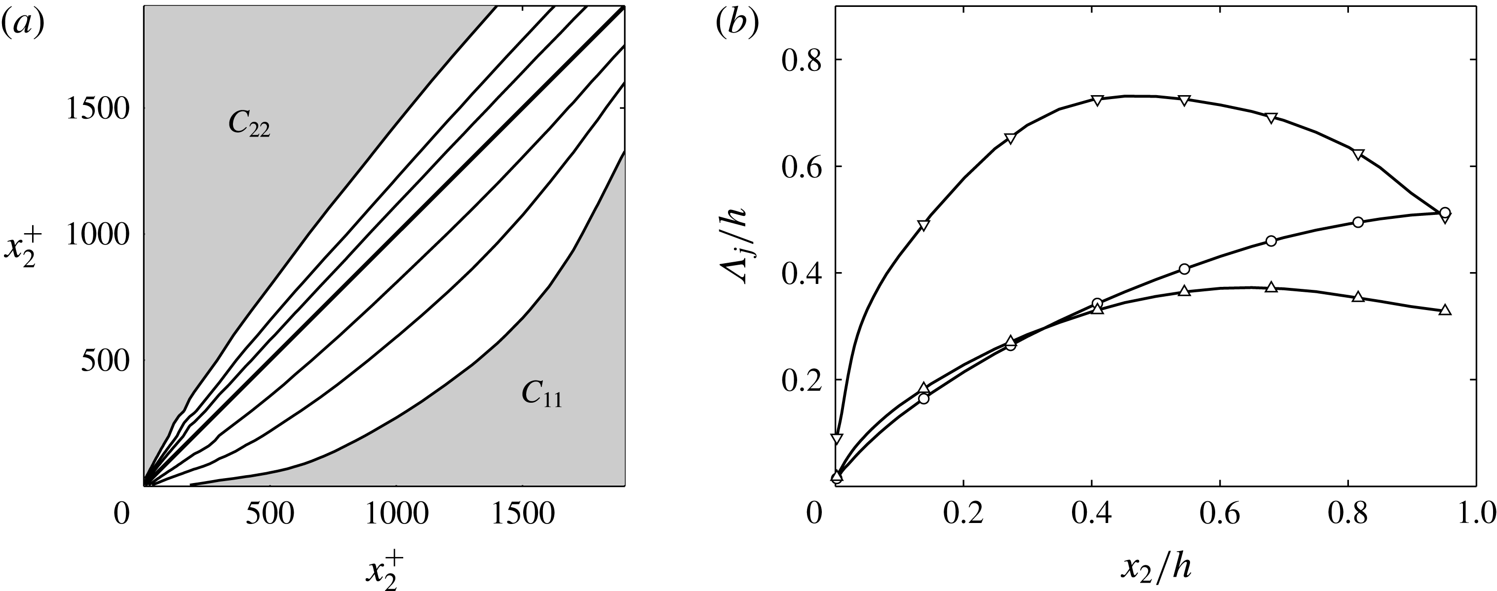
 $C_{11}$
near the opposite wall. The streamwise-velocity eddies are large enough to be ‘global’, involving the whole channel. Although the energy considerations in § 3.2 imply that the
 $u_{1}$
streak and the cross-flow rollers have to be related, and we shall see later that they appear together in conditional flow fields, the difference in their size makes it difficult to describe them as parts of a single eddy. At the very least, each streak must contain several rollers. It should also be noted at this point that, because the correlations are second-order quantities, they favour the locations and times where the velocity is strongest, which need not occur simultaneously for all the velocity components.
The correlation functions for the cross-flow velocities are relatively independent of the Reynolds number, and vary little among the flows in which they have been studied (Sillero et al.
Reference Sillero, Jiménez and Moser2014). They are good candidates for ‘universal’ features of shear flows. Those of
 $u_{1}$
are not, and are known with less certainty. The lengths implied by figure 9(c) for channels
 $(\unicode[STIX]{x1D706}_{1}\approx 20h)$
are, unfortunately, comparable to the length of the computational box
 $(L_{1}=25h)$
, and vary by
 $\pm 20\,\%$
among different simulations, including those performed within the same research group using similar codes (Sillero et al.
Reference Sillero, Jiménez and Moser2014). Experiments are also ambiguous because it is difficult to deduce long spatial dimensions from temporal data, or to collect spatial measurements over very long distances. Nevertheless, the lengths in figure 9(a) are probably approximately correct. A simulation in a very large box
 $(L_{1}=190h)$
was performed by Lozano-Durán & Jiménez (Reference Lozano-Durán and Jiménez2014a
) at
 $h^{+}=550$
, and did not result in longer eddies. The length-to-width ratio,
 $\unicode[STIX]{x1D706}_{1}/\unicode[STIX]{x1D706}_{3}\approx 8$
, of the spectral ridge in figure 7(a) is consistent with
 $\unicode[STIX]{x1D706}_{1}=16h$
for streaks of width
 $\unicode[STIX]{x1D706}_{3}=2h$
, which is the maximum value implied by the cross-flow section in figure 9(c). This width is much narrower than the spanwise dimensions of the computational box, and there is no reason to believe that it is numerically constrained. The shorter end of the spectral ridge in figure 7(a) is also short with respect to the computational box, and its aspect ratio should not be numerically constrained. The fact that it does not change with the Reynolds number, which modifies the ratio between the length of these streaks and the size of the box, and that the aspect ratio of the shorter streaks is similar to that of the longer streaks, gives some confidence on the results for the longer eddies.
On the other hand, the correlation length of
 $u_{1}$
in boundary layers is shorter than in channels,
 $\unicode[STIX]{x1D706}_{1}\approx 4h$
(Sillero et al.
Reference Sillero, Jiménez and Moser2014), while that in Couette flows appears to be longer than any of the experiments or simulations that have been performed; it might be infinite (Pirozzoli et al.
Reference Pirozzoli, Bernardini and Orlandi2014). The reason for these differences is unclear, although reasonable models can be advanced in some cases. For example, very long streaks presumably require very long times to organise (see the discussion of figure 29 in § 6.1). Visually tracking the large scales in simulations of channels confirms that they evolve extremely slowly, with evolution times of the order of many turnovers,
 $tu_{\unicode[STIX]{x1D70F}}/h\gg 1$
. Assuming that the relevant deformation velocity is
 $u_{\unicode[STIX]{x1D70F}}$
, the time needed to organise an eddy of length
 $\unicode[STIX]{x1D706}_{1}$
is
 $\unicode[STIX]{x1D706}_{1}/u_{\unicode[STIX]{x1D70F}}$
, during which time the flow is advected approximately by
 $U_{b}\unicode[STIX]{x1D706}_{1}/u_{\unicode[STIX]{x1D70F}}\approx 30\unicode[STIX]{x1D706}_{1}$
. In a uniform channel, very long advection lengths are available, but, in a boundary layer, a streak of length
 $\unicode[STIX]{x1D706}_{1}=4h$
would be advected by approximately
 $100h$
during its formation. Over that distance, the thickness of the boundary layer grows by a factor of two. In essence, streaks in boundary layers do not have time to become very long before the mean velocity profile changes enough to require them to adapt to a new size. A similar argument could explain the scatter among the measured correlation lengths of different channel simulations, because not all of them are run for the same time. The streaks that we see in channels could still be slowly growing in some cases. This problem also applies to the development length of laboratory experiments.
Hutchins & Marusic (Reference Hutchins and Marusic2007) have proposed that real streamwise-velocity eddies may be very long, meandering on a shorter scale. They note that the meanders hide the real length of the streaks in spectra and correlations, and they present visual evidence of lengths of
 $20h$
in boundary layers, meandering at the spectrally measured length of
 $6h$
. Unfortunately, their argument does not explain why channels or Couette flows should meander less than boundary layers, and thus appear longer in the spectra. Neither do the estimates of the evolution time in the previous paragraph explain the differences between Couette flow and channels. The question of the real length of the large velocity streaks in wall-bounded turbulence, and the reasons for it, remain at the moment unsettled. This question will be revisited when discussing individual velocity structures in § 5.3.
3.6 Filtered correlations
(a) One-dimensional two-point correlation,
 $C_{(2)}(x_{2},\tilde{x}_{2})$
, as a function of
 $x_{2}$
. Above the diagonal,
 $C_{(2)22}$
. Below the diagonal,
 $C_{(2)11}$
. Contours are
 $C_{(2)}=[0.3,0.5,0.7,1]$
. (b) Correlation depth at
 $C_{(2)}=0.3$
of the different velocity components, as a function of the distance from the wall to the reference point. ▵,
 $u_{1}$
;
 $\circ$
,
 $u_{2}$
; ▿,
 $u_{3}$
. Channel CH2000.

Consider next the question of defining the correlation depth of the velocities at different distances from the wall. In channels, we can define a one-dimensional vertical correlation profile,
 $$\begin{eqnarray}C_{(2)ii}(x_{2},\tilde{x}_{2})=\max _{\unicode[STIX]{x0394}x_{1}}C_{ii}(\unicode[STIX]{x0394}x_{1},x_{2},\tilde{x}_{2}),\end{eqnarray}$$
where the value at
 $\unicode[STIX]{x0394}x_{1}=0$
is substituted by the maximum over
 $\unicode[STIX]{x0394}x_{1}$
to take into account the inclination of the correlations. This quantity is represented in figure 10(a) for
 $u_{1}$
and
 $u_{2}$
, using the symmetry of
 $C_{(2)}$
with respect to its two arguments to include the two velocity components in the same figure.
There are many ways of defining the correlation depth,
 $\unicode[STIX]{x1D6EC}_{j}(\tilde{x}_{2})$
, of
 $u_{j}$
at a given distance from the wall, but the simplest way is to measure the width at a given level of the correlation profile centred at
 $\tilde{x}_{2}$
. Figure 10(b) displays the correlation depth defined at
 $C_{(2)ii}=0.3$
for the three velocity components. It is evident that
 $u_{1}$
is deeper than
 $u_{2}$
or
 $u_{3}$
, and that all the velocities are more deeply correlated away from the wall than near it. But it is difficult to extract other conclusions from the figure. In particular, since the spectra in figure 7(d–f) show that all the velocity components get longer as they move away from the wall, it is unclear from figure 10(b) whether the growth in depth is due to the differences in wall distance, or to the longer eddies. An interesting related question, when the reference point
 $\tilde{x}_{2}$
is chosen in the buffer layer, is how far from the wall are the eddies responsible for the spectral ridge in figure 7(a).
Fortunately, the Fourier duality between covariances and spectra along homogeneous directions allows us to filter the covariance to only include a restricted range of wall-parallel wavelengths.
Consider a generic variable,
 $u$
, whose covariance is
 $R_{uu}(\unicode[STIX]{x0394}x_{1},x_{2},\tilde{x}_{2})$
. Its spectrum,
 $E_{uu}(k_{1},x_{2},\tilde{x}_{2})=\langle \widehat{u}(k_{1},x_{2})\widehat{u}^{\ast }(k_{1},\tilde{x}_{2})\rangle$
, is the Fourier transform of
 $R_{uu}$
(see appendix B.2). This is true for any spectrum. In particular, if we apply to
 $\widehat{u}$
a spectral filter
 $G(k_{1})$
that restricts it to some range of wavenumbers,
 $\overline{\widehat{u}}(k_{1})=\widehat{u}(k_{1})G(k_{1})$
, its spectrum is similarly filtered to
 $E_{\bar{u}\bar{u}}(k_{1},x_{2},\tilde{x}_{2})=E_{uu}(k_{1},x_{2},\tilde{x}_{2})|G(k_{1})|^{2}$
. The covariance of the filtered variable can then be obtained as the inverse Fourier transform of the filtered spectrum. A similar procedure can be applied to
 $k_{3}$
and to three-dimensional covariances.
Two-dimensional sections through the reference point
 $(\tilde{x}_{2}/h=0.35)$
of the two-point filtered autocorrelation function of the streamwise velocity. (a)
 $\unicode[STIX]{x1D706}_{1}/h\in (1.4,2.2)$
, (b)
 $(5.0,8.2)$
and (c)
 $(13.6,22.0)$
. Contours are
 $C_{11}=\pm [1,2]$
, and negative contours are dashed. (d) One-dimensional filtered correlation,
 $C_{(2)11}(x_{2},\tilde{x}_{2};\unicode[STIX]{x1D706}_{1})$
, of the streamwise velocity, as a function of the distance from the wall. Above the diagonal, as in (a). Below the diagonal, as in (b). Contours are
 $C_{(2)11}=[0.3,0.5,1]$
. (e) Correlation depth of
 $u_{1}$
, as a function of the central filter wavelength. Each pair of lines represents the upper and lower limits within which
 $C_{(2)11}>0.4$
.
 $\tilde{x}_{2}=[15/h^{+},0.1,0.2,0.35,0.6]$
, as marked by their common origin at
 $\unicode[STIX]{x1D706}_{1}=0$
. The circles are
 $x_{2}=0.03\unicode[STIX]{x1D706}_{1}$
. Channel CH2000.

Filtered correlation functions can be defined by normalising the covariance with the standard deviation of the filtered variables, but it is more useful to normalise them with the total fluctuation intensities,
 $$\begin{eqnarray}C_{\bar{u}\bar{u}}(\boldsymbol{x},\tilde{\boldsymbol{x}})=\frac{\langle \overline{u}(\boldsymbol{x})\overline{u}(\tilde{\boldsymbol{x}})\rangle }{u^{\prime }(x_{2})u^{\prime }(\tilde{x}_{2})}\,(N_{bands}).\end{eqnarray}$$
This has the advantage of keeping some spectral information about the relative intensity of the filtered variable in the different wavenumber ranges, but at the price of lacking a well-defined maximum value. The value of
 $C_{\bar{u}\bar{u}}$
at
 $\boldsymbol{x}=\tilde{\boldsymbol{x}}$
is the relative energy of the filtered variable with respect to the total. In (3.15), and in the figures in the rest of this section, we have assumed that the filter is used to separate the flow into
 $N_{bands}$
approximately equal logarithmic bands, and we have multiplied the filtered correlations by
 $N_{bands}$
to get maxima of order unity. Even so, the filtered correlations of the different variables reach different maximum levels, and the threshold used to determine correlation depths has to be adjusted to some fraction of the empirical maximum of each case.
Using these definitions, the effect of filtering the
 $C_{11}$
correlation in figure 9(c) is shown in figure 11(a–c). The streamwise coordinate is filtered with a family of self-similar sharp spectral box filters in which the maximum and minimum wavelengths differ by a factor of 1.6. The central filter wavelength increases from figure 11(a) to 11(c), and the longest filter spans roughly half of the length of the computational box. It can be shown that the streamwise average of any correlation which does not include
 $k_{1}=0$
has to vanish, and all the filtered correlations in figure 11 are oscillatory. As the central wavelength is made shorter, the depth of the correlation decreases, until it eventually separates from the wall.
This is made clearer by the correlation profile
 $C_{(2)11}(x_{2},\tilde{x}_{2};\unicode[STIX]{x1D706}_{1})$
in figure 11(d), built from the filtered correlations in figure 11(a,b), which should be compared with the unfiltered figure 10(a). The main difference between the two figures is that the depth of the filtered correlations in figure 11(d) is more independent of
 $\tilde{x}_{2}$
than it was in figure 10(a). Moreover, different filter wavelengths produce very different depths, answering the question of whether the correlation depth is linked to the length of the eddies or to their distance from the wall.
Figure 11(e) displays the minimum and maximum distances from the wall at which the filtered correlation profiles exceed the arbitrary threshold
 $C_{(2)11}=0.4$
. The depth at short wavelengths is very small, and the maximum and minimum heights coincide. As the central wavelength of the filter increases, so does the depth, and the lower limit reaches the wall at some wavelength that depends on the reference height
 $\tilde{x}_{2}$
. Eddies longer than that limit ‘attach’ to the wall and link directly the inner- and outer-flow regions. The solid line starting near the origin in figure 11(e) corresponds to the upper correlation limit of eddies centred at
 $\tilde{x}_{2}^{+}=15$
, and marks the depth of the correlated wall layer as a function of the streamwise wavelength. It grows approximately linearly as
 $x_{2}\approx \unicode[STIX]{x1D706}_{1}/30$
, until it saturates to
 $x_{2}\approx 0.3h$
for very long wavelengths. The slope of this line depends on the correlation level used to define the depth, but it is clear from figure 11(e) that other thresholds behave similarly. For short wavelengths,
 $\unicode[STIX]{x1D706}_{1}^{+}\lesssim 2000$
, the correlation depth settles to approximately
 $x_{2}^{+}\approx 30$
, and the vertically correlated layer does not extend above the buffer layer. Similarly defined coherence limits for the three velocity components have been incorporated as grey patches to the spectra in figure 7(d–f).
It is interesting to note that a large coherence depth is a property of long eddies, independently of whether they are attached to the wall or not. For example, the pair of lines corresponding to
 $\tilde{x}_{2}=0.6$
in figure 11(e) define a correlation depth spanning half of the channel for wavelengths that are much shorter than the wavelength at which this particular correlation attaches to the wall,
 $\unicode[STIX]{x1D706}_{1}\approx 15h$
. The message of figure 11(e) is that long eddies are also deep. They attach to the wall when they grow to be too deep to do otherwise, but they do not appear to originate from the wall.
3.7 The effect of the Reynolds number
(a) Sketch of attached and detached eddies in a channel, created with independent random sizes and positions. The thicker (red) objects are attached. (b) Maximum value of the velocity fluctuation intensities. Various experimental and numerical flows: open symbols,
 $u_{1}^{\prime 2^{+}}$
; closed,
 $u_{2}^{\prime 2^{+}}$
; light blue fill,
 $u_{3}^{\prime 2^{+}}$
. ▿, Boundary layers; ▵, channels;
 $\circ$
, pipes. Each velocity component has been offset by a different constant, so that the trend lines cross zero at
 $h^{+}=100$
. The trend lines are:
 $u_{1}^{\prime 2^{+}}=3.58+0.65\log h^{+}$
,
 $u_{2}^{\prime 2^{+}}=0.51+0.1\log h^{+}$
, and
 $u_{3}^{\prime 2^{+}}=-0.60+0.4\log h^{+}$
. (c) Correlation limits for
 $\tilde{x}_{2}/h=0.6$
, as functions of the central filter wavelength. ▿,
 $C_{(2)11}=0.4$
; ▵,
 $C_{(2)33}=0.25$
; ▫,
 $C_{(2)pp}=0.25$
. Each pair of lines represents the upper and lower limits within which
 $C_{(2)}$
exceeds the specified level. (d) One-dimensional streamwise spectral density of the pressure, as a function of the wall distance. The two diagonals are approximately: ——,
 $\unicode[STIX]{x1D706}_{I}=x_{2}$
; - - - -,
 $\unicode[STIX]{x1D706}_{I}=5x_{2}$
, reduced to
 $\unicode[STIX]{x1D706}_{1}$
assuming
 $\unicode[STIX]{x1D706}_{1}\approx \unicode[STIX]{x1D706}_{3}$
. The grey patch is the region vertically correlated with the wall. Channel CH2000.

The resulting organisation of the velocity eddies is sketched in figure 12(a). Eddies of all sizes can be found at all heights, but they cannot grow larger than their distance from the wall. Statistically, this means that the size of the largest eddies scales linearly with the wall distance.
The relevance of attached eddies was first stressed by Townsend (Reference Townsend1961) and developed by Perry, Henbest & Chong (Reference Perry, Henbest and Chong1986). They noted that, if the intensity of eddies centred within the logarithmic layer scales with
 $u_{\unicode[STIX]{x1D70F}}$
, and if those eddies retain their intensity down to the wall, the fluctuation energy near the wall should increase with the logarithm of the Reynolds number. The argument hinges on the approximately uniform long-wavelength spectral ‘skirt’ of
 $\unicode[STIX]{x1D719}_{11}$
and
 $\unicode[STIX]{x1D719}_{33}$
in figure 7(d,f). It does not apply to
 $\unicode[STIX]{x1D719}_{22}$
, where the damping of
 $u_{2}$
by the impermeability condition ensures that the near-wall coherent layer in figure 7(e) contains no energy at long wavelengths.
It can be shown that the longest wavelengths of the spectra in figure 7 scale in outer units, while their short-wavelength end scales in wall units. The range of energy-containing eddies near the wall thus scales like
 $\unicode[STIX]{x1D706}_{max}/\unicode[STIX]{x1D706}_{min}\sim h^{+}$
, and the total fluctuation energy is
 $\int \unicode[STIX]{x1D719}\,\text{d}(\log \unicode[STIX]{x1D706}_{1})\sim \log (h^{+})$
. Figure 12(b) shows that this is true for the maxima of
 $u_{1}^{\prime 2+}$
and
 $u_{3}^{\prime 2+}$
, but not (or much more weakly) for
 $u_{2}^{\prime 2+}$
.
Figure 12(c) shows the vertical correlation limits of
 $u_{1}$
and
 $u_{3}$
for eddies centred at one particular location in the outer layer
 $(\tilde{x}_{2}=0.6h)$
. The main difference between the two variables in this figure is that, while the depth of
 $u_{1}$
increases with the wavelength over the whole range of the figure, that of
 $u_{3}$
only grows up to
 $\unicode[STIX]{x1D706}_{1}\approx 3h$
, beyond which the energy of
 $u_{3}$
decreases, and the filtered correlation becomes too weak to show at the selected threshold. As a consequence, the wall-attached eddies of
 $u_{1}$
eventually fill the whole channel in figure 7(d), but those of
 $u_{3}$
never reach above
 $x_{2}/h\approx 0.2$
in figure 7(f).
More surprising is the correlation depth of the pressure, which is included in figure 12(c) and in the pressure spectrum in figure 12(d). The pressure is an attached variable, with deep eddies that span a large fraction of the channel, but only at the comparatively short wavelengths of the
 $(u_{2},u_{3})$
eddies discussed in figure 9. Given the irrotational character of the longest
 $u_{1}$
eddies, whose vorticity is very low, one would expect their dynamics to be mainly controlled by the pressure. Indeed, the pressure correlation and the pressure spectrum are long, but the correlation in figure 12(c) gets thinner for the longer wavelengths, and detaches from the wall. Figure 12(d) shows that only a very weak vertical correlation of the pressure reaches the wall beyond
 $\unicode[STIX]{x1D706}_{1}\approx 5h$
. The implication is that the near-wall long and wide eddies in the spectral ridge of figure 7(a) are mostly maintained by weak but persistent Reynolds stresses. The pressure appears to be mostly associated with the rollers discussed in figure 9.
Figures 7(d) and 7(f) show that arguments similar to those above imply that the fluctuation profile above the buffer layer should be
 $u_{j}^{\prime 2+}\sim \log (h/x_{2})$
, for
 $u_{1}$
and
 $u_{3}$
. Both predictions have been confirmed observationally: by numerical simulations in the case of
 $u_{3}$
(Jiménez & Hoyas Reference Jiménez and Hoyas2008), and experimentally in the case of
 $u_{1}$
(Marusic et al.
Reference Marusic, Monty, Hultmark and Smits2013).
It should be mentioned at this point that there is some controversy about the behaviour of even basic flow statistics at very high Reynolds numbers
 $(h^{+}\gtrsim 10^{4})$
. This range is still inaccessible to simulations, and hard to measure experimentally. For example, the presence of an ‘outer’ kinetic energy peak in the middle of the logarithmic layer has been variously reported (Smits et al.
Reference Smits, McKeon and Marusic2011) as an outer maximum of the total fluctuation intensity, or as a peak in the spectral energy density. The two claims are different, and both have proved hard to confirm by high-resolution experiments (Örlü et al.
Reference Örlü, Fiorini, Segalini, Bellani, Talamelli and Alfredsson2017). The second claim, a peak in the spectral density
 $\unicode[STIX]{x1D719}_{11}$
, could be due either to a peak in the total energy (the first claim), or to the concentration of the same energy into a narrower range of wavelengths. The latter would be a natural consequence of the narrowing of the spectrum as the flow gets closer to a single scale far from the wall (see figure 7
e), presumably because, as discussed in § 3.1, this layer has a natural unit of length. However, in the absence of unambiguous experimental confirmation, it is possible that a different kind of eddies than those described here exists at high Reynolds numbers, and that they are not captured by the simulations used in this article.
Summarising the results up to now, we have shown that the one- and two-point statistics of wall-bounded turbulent flows suggest the existence of two types of eddies: a self-similar family of inclined large-scale rollers that mostly involve the transverse-velocity components, and which are restricted to the logarithmic layer; and the much longer streaks of the streamwise velocity, also self-similar in the spanwise direction, that exists at all heights from the wall. The largest of these streaks fill most of the width of the flow. For sizes
 $\unicode[STIX]{x1D706}_{I}\gtrsim x_{2}$
, both types of eddies interact directly with the shear, and are therefore presumably involved in the energy-generation cycle, but their very different sizes suggest that they are only indirectly related to one another. Long eddies are deep in the wall-normal direction, but only attach to the wall if they become so large that they do not fit into the flow otherwise. Examples of structures of the transverse velocities are given later in figures 20 and 21. Examples of streaks are figure 23.
4 Eddies and coherence
We noted in the introduction that our definitions of eddies and structures are conceptually different, because the former are statistical constructs while the latter should also include dynamics. Most of our discussion up to now applies to eddies rather than to structures, since we have made very few references to temporal evolution. Even so, being able to describe eddies as particularly probable states of the flow is useful, and many techniques have been developed for doing it. A short summary of the methods used in this review, and of their relation to one another, is in appendix B. In this section we collect some useful results about eddies, and start investigating their temporal evolution. We will then be in a position to classify the parameter plane of eddy size and wall distance in terms of where the different dynamical models are most likely to apply, although we delay to § 5 the consideration of coherent structures.
The definition of eddies depends, to some extent, on the application for which they are intended. As mentioned in the introduction, the question of whether the flow can be described in terms of eddies recalls the wave–particle duality of quantum mechanics. The problem is there how to describe ‘ostensibly’ localised objects, such as particles, in terms of extended fields, while our problem is how to describe an ostensibly field-like flow in terms of localised structures. Turbulent flows are often expressed as Fourier expansions because sines and cosines have well-defined wavelengths, and size is a crucial aspect of the turbulence problem (Richardson Reference Richardson1920). However, the Fourier basis functions are spatially homogeneous and do not describe location. Conversely, points are perfectly localised, but have no size. A packet of several Fourier modes can be localised, but only at the expense of some spread
 $\unicode[STIX]{x0394}k$
in its wavenumber. This is related to the spread
 $\unicode[STIX]{x0394}x$
of its position by the uncertainty relation (Gasquet & Witomski Reference Gasquet and Witomski1998),
 $\unicode[STIX]{x0394}k\unicode[STIX]{x0394}x\gtrsim O(1)$
; but this is only a lower bound. Most superpositions of wavetrains of different wavelengths have no obvious spatial structure (see figure 30 in appendix B.2). A definition that has often been proposed for an ‘eddy’ is a Fourier packet for which the above inequality is satisfied as tightly as possible (Tennekes & Lumley Reference Tennekes and Lumley1972). Algorithmic definitions have been given, for example, by Berkooz, Holmes & Lumley (Reference Berkooz, Holmes and Lumley1993), who approximate the covariance as a superposition of randomly distributed compact eddies, or by Moin & Moser (Reference Moin and Moser1989), who construct ‘most-compact’ eddies by adjusting the relative phases of several proper orthogonal (POD) modes. This last method is described in appendix B.2, and has been used to construct the eddies in figure 13(a–d).
(a–d) Most-compact eddies for pressure and for the individual velocity components, as discussed in the text, normalised to unit maximum amplitude and computed from correlations in the half-channel
 $x_{2}<h$
, filtered in the band
 $\unicode[STIX]{x1D706}_{1}/h=1.4{-}2.2$
. Black patches are
 $u_{j,mc}>0.5$
, and grey patches are
 $u_{j,mc}<-0.5$
. Channel CH2000. (a)
 $p$
. (b)
 $u_{1}$
. (c)
 $u_{2}$
. (d)
 $u_{3}$
. (e) Profiles of the maximum eddy amplitude for
 $u_{1}$
, as functions of the wall distance. Filter bands centred at: ——,
 $\unicode[STIX]{x1D706}_{1}^{+}=280$
; - - - -,
 $\unicode[STIX]{x1D706}_{1}/h=1.0$
; – ⋅ – ⋅ –,
 $\unicode[STIX]{x1D706}_{1}/h=1.8$
;
 $\cdots \cdots$
,
 $\unicode[STIX]{x1D706}_{1}/h=6.5$
. (f) Height of the centre of gravity of the compact eddies computed from the leading PODs, in outer scaling. The two thicker diagonals are approximately: ——,
 $\unicode[STIX]{x1D706}_{I}=\bar{x}_{2,j}$
; - - - -,
 $\unicode[STIX]{x1D706}_{I}=5\bar{x}_{2,j}$
, reduced to
 $\unicode[STIX]{x1D706}_{1}$
assuming
 $\unicode[STIX]{x1D706}_{1}\approx \unicode[STIX]{x1D706}_{3}$
. Channels: ——,
 $h^{+}=550$
(del Álamo et al.
Reference del Álamo, Jiménez, Zandonade and Moser2004); - - - -, CH950; – ⋅ – ⋅ –, CH2000. ▫,
 $p$
; ▿,
 $u_{1}$
;
 $\circ$
,
 $u_{2}$
; ▵,
 $u_{3}$
. (g) As in (f), in wall units.

POD modes are optimal basis functions,
 $\unicode[STIX]{x1D753}_{(\unicode[STIX]{x1D6FC})}$
, which provide an expansion of the flow that approximates the covariance with as few degrees of freedom as possible,
 $$\begin{eqnarray}\boldsymbol{u}(\boldsymbol{x})=\mathop{\sum }_{\unicode[STIX]{x1D6FC}}\widehat{\boldsymbol{u}}_{(\unicode[STIX]{x1D6FC})}\unicode[STIX]{x1D753}_{(\unicode[STIX]{x1D6FC})}(\boldsymbol{x}).\end{eqnarray}$$
Unfortunately, it is shown in appendix B.1 that the PODs are Fourier modes along homogeneous coordinate directions,
 $$\begin{eqnarray}\unicode[STIX]{x1D753}_{(\unicode[STIX]{x1D6FC},\boldsymbol{k})}(\boldsymbol{x})=\widehat{\unicode[STIX]{x1D753}}_{(\unicode[STIX]{x1D6FC})}(x_{2})\exp [\text{i}(k_{1}x_{1}+k_{3}x_{3})],\end{eqnarray}$$
and are therefore poor representations of coherent structures.
The POD modes are eigenfunctions of the two-point covariance. The eigenvalue of the eigenfunction (4.2) measures the average contribution to the variance of the corresponding term of the expansion (4.1), and it is typically true that the first few eigenvalues account for most of the variance. The eddies in figure 13(a–d) are constructed using the leading (i.e. highest eigenvalue) PODs,
 $\unicode[STIX]{x1D719}_{(1)j}$
, of the filtered correlations in figure 11. For this case, the most-compact eddy of
 $u_{1}$
contains approximately 30 % of the total energy of the filtered
 $u_{1}$
. Those of
 $u_{2}$
and
 $u_{3}$
contain approximately 45 % in both cases. The corresponding percentages for the sum of the first five PODs are 80 % for
 $u_{1}$
, and 90 % for the two transverse components. These percentages increase for filters with longer wavelengths, and decrease for shorter wavelengths.
The most-compact eddies do not form an orthogonal basis, as the PODs do, nor are they optimum in the sense of generating a most efficient expansion, because they are sums of eigenfunctions that are only optimal for a single wavenumber. Therefore, they are not very useful for constructing global reduced-order models of the flow. They represent the most localised eddies whose covariance approximates the two-point covariance of the flow, and they are useful in constructing the local models discussed in the introduction as one of the reasons to consider coherent structures. Their streamwise shape depends on the window used to filter the covariance from which they are obtained. The eddies in figure 13(a–d) could be made to contain fewer side bands by choosing a wider filter, but only at the expense of making their vertical structure less representative of the flow, because they would mix PODs with more diverse vertical structure. Conversely, they could be made more representative of a single POD by choosing a narrower filter, but only at the expense of increasing the number of side bands. Filters such as those used in figure 13(a–d), in which the wavenumber interval is approximately half the central wavenumber, are probably a good compromise in most cases.
Figure 13(e) shows the wall-normal structure of the maximum over
 $x_{1}$
,
 $$\begin{eqnarray}u_{1,max}(x_{2};\unicode[STIX]{x1D706}_{1})=\max _{x_{1}}u_{1,mc}(x_{1},x_{2};\unicode[STIX]{x1D706}_{1}),\end{eqnarray}$$
of the most-compact eddies,
 $u_{1,mc}$
. They are constructed from correlations which have been filtered over bands with various central wavelengths and uniform relative width in Fourier space
 $(\unicode[STIX]{x1D706}_{1,max}/\unicode[STIX]{x1D706}_{1,min}\approx 1.6)$
. The profile defined in (4.3) plays the same role as the one-dimensional correlation profile defined in (3.14) and, as in that case, longer wavelengths are vertically deeper. This is quantified in figure 13(f,g) by the centre of gravity of the wall-normal distribution,
 $$\begin{eqnarray}\bar{x}_{2,j}=\frac{\displaystyle \int _{0}^{h}x_{2}u_{j,max}\,\text{d}x_{2}}{\displaystyle \int _{0}^{h}u_{j,max}\,\text{d}x_{2}}.\end{eqnarray}$$
Figure 13 shows that eddies separate into a short family (for
 $u_{2}$
,
 $u_{3}$
and
 $p$
) in which
 $\unicode[STIX]{x1D706}_{I}\approx \bar{x}_{2,j}$
, and a longer family for
 $u_{1}$
in which
 $\unicode[STIX]{x1D706}_{I}\approx 5\bar{x}_{2,1}$
. These two trend lines, plotted either in terms of
 $\unicode[STIX]{x1D706}_{1}$
or of
 $\unicode[STIX]{x1D706}_{I}$
, have been incorporated in all the figures containing spectra in this article, for reference. The shorter line,
 $\unicode[STIX]{x1D706}_{I}\approx \bar{x}_{2}$
, is the Corrsin length, below which the flow decouples from the energy-containing eddies. The longer line coincides with the approximate position of the core of the
 $\unicode[STIX]{x1D719}_{11}$
energy spectrum. Most of the energy of the two transverse-velocity components is contained between these two lines. Figures 13(f) and 13(g) show that short and shallow eddies scale in wall units, while long and tall eddies scale in outer units. Although not shown in the figure, the eddies of
 $u_{1}$
and
 $p$
remain attached to the wall at all wavelengths (see figure 13
e), those of
 $u_{2}$
have negligible energy near the wall and are always detached, and those of
 $u_{3}$
detach for
 $\unicode[STIX]{x1D706}_{1}/h\gtrsim 2$
.
4.1 Advection velocities
We have not discussed up to now the temporal evolution of eddies, but whether they can be considered coherent or not depends on whether they are able to keep their shape for dynamically significant times. This depends, among other things, on how their propagation velocity changes with the wavenumber and with the location along inhomogeneous directions.
Consider a variable
 $\unicode[STIX]{x1D712}$
that we wish to approximate as a wave with phase velocity
 $c_{\unicode[STIX]{x1D712}}$
along the direction
 $x_{1}$
. A simple definition of the phase velocity was introduced by del Álamo & Jiménez (Reference del Álamo and Jiménez2009) by minimising
 $\langle (\unicode[STIX]{x2202}_{t}\unicode[STIX]{x1D712}+c_{\unicode[STIX]{x1D712}}\unicode[STIX]{x2202}_{1}\unicode[STIX]{x1D712})^{2}\rangle$
. The result is
 $$\begin{eqnarray}c_{\unicode[STIX]{x1D712}}=-\frac{\langle \unicode[STIX]{x2202}_{t}\unicode[STIX]{x1D712}\unicode[STIX]{x2202}_{1}\unicode[STIX]{x1D712}\rangle }{\langle (\unicode[STIX]{x2202}_{1}\unicode[STIX]{x1D712})^{2}\rangle },\end{eqnarray}$$
which can be expressed as
 $$\begin{eqnarray}c_{\unicode[STIX]{x1D712}}(k)=-\frac{\text{Im}\langle k_{1}\widehat{\unicode[STIX]{x1D712}}^{\ast }\unicode[STIX]{x2202}_{t}\widehat{\unicode[STIX]{x1D712}}\rangle }{\langle k_{1}^{2}|\widehat{\unicode[STIX]{x1D712}}|^{2}\rangle }\end{eqnarray}$$
for individual Fourier modes, where the asterisk stands for complex conjugation, and
 $\text{Im}$
for the imaginary part.
Denoting by
 $c_{j}$
the advection velocity of the
 $u_{j}$
velocity component, the spectral phase velocity of the streamwise-velocity component,
 $c_{1}$
, is shown in figure 14 at three heights in the channel, normalised with the mean flow velocity at each height. Del Álamo & Jiménez (Reference del Álamo and Jiménez2009) showed that the phase velocity agrees with the local velocity for most wavelengths, except for very large scales, where
 $c_{1}\approx U_{b}$
independently of
 $x_{2}$
, and in the buffer layer, where
 $c_{1}^{+}\approx 11$
. Figure 14 shows that this remains approximately true in the present case, at a higher Reynolds number than in del Álamo & Jiménez (Reference del Álamo and Jiménez2009), and that the scale dependence is reasonably well described as a function of the wall-parallel isotropic wavelength
 $\unicode[STIX]{x1D706}_{I}$
.
Figure 15(a) summarises the wall-normal dependence of
 $c_{1}$
, and shows that the transition to the large-scale behaviour in which the eddies do not follow the flow takes place at
 $\unicode[STIX]{x1D706}_{I}\approx 5x_{2}$
above
 $x_{2}^{+}\approx 100$
. Closer to the wall, the transition wavelength saturates at
 $\unicode[STIX]{x1D706}_{I}^{+}\approx 10^{3}$
, which is also the boundary in figure 7(a) between the near-wall spectral energy component and the self-similar outer ridge. A similar behaviour is found for the other two velocity components, although there is very little large-scale energy in the case of
 $u_{2}$
.
Phase velocity for
 $u_{1}$
normalised with the mean velocity at each height,
 $c_{1}/U_{1}(x_{2})$
. Channel CH2000. Contours are spaced by 0.1, drawn only where the spectral density
 $\unicode[STIX]{x1D719}_{11}$
is greater than 2 % of its maximum. (a)
 $x_{2}^{+}=15$
. (b)
 $x_{2}^{+}=80$
; (c)
 $x_{2}/h=0.15\,(x_{2}^{+}=300)$
. The hyperbola-like thicker lines are: ——,
 $\unicode[STIX]{x1D706}_{I}=x_{2}$
; - - - -,
 $\unicode[STIX]{x1D706}_{I}=5x_{2}$
.

Advection velocity parameters for
 $u_{1}$
in channels, as a function of
 $x_{2}$
, averaged over shells of constant
 $\unicode[STIX]{x1D706}_{I}$
. Shaded contours are CH2000. The thicker lines are: – ⋅ – ⋅ –,
 $h^{+}=550$
(del Álamo et al.
Reference del Álamo, Jiménez, Zandonade and Moser2004); - - - -, CH950; ——, CH2000. (a) Phase velocity normalised with the mean flow velocity. Shaded contours are
 $c_{1}/U_{1}(x_{2})=0.9(0.1)1.4$
, and thick lines are
 $c_{1}/U_{1}(x_{2})=1$
. (b) Wavenumber dispersion parameter, as defined in (4.8). Shaded contours are
 $c^{\ast }=1.0(0.3)2.2$
, and thick lines are
 $c_{1}^{\ast }=1$
. (c) Shearing parameter, as defined in (4.9). Shaded contours are
 $\unicode[STIX]{x1D6FE}_{s1}=0.2(0.2)1.0$
, and thick lines are
 $\unicode[STIX]{x1D6FE}_{s1}=0.2$
. The straight lines in (a–c) are: ——,
 $\unicode[STIX]{x1D706}_{I}=x_{2}$
; - - - -,
 $\unicode[STIX]{x1D706}_{I}=5x_{2}$
and
 $x_{2}^{+}=80$
. (d) Instantaneous snapshots of an attached logarithmic-layer ejection in a channel at
 $h^{+}=4200$
. The flow (and time) goes from left to right, and the streamwise displacement of the structure has been shortened in order to fit its complete lifetime in the figure. The structure is coloured with the distance from the wall. Reproduced with permission from Lozano-Durán & Jiménez (Reference Lozano-Durán and Jiménez2014b
).

The propagation velocity of wave packets is the group velocity (Whitham Reference Whitham1974),
 $$\begin{eqnarray}c_{g\unicode[STIX]{x1D712}}(k)=\unicode[STIX]{x2202}_{k_{1}}(k_{1}c_{\unicode[STIX]{x1D712}})=c_{\unicode[STIX]{x1D712}}+k_{1}\unicode[STIX]{x2202}_{k_{1}}c_{\unicode[STIX]{x1D712}}.\end{eqnarray}$$
The difference between the phase and group velocities is generally small, but significant. For example, it was shown by del Álamo & Jiménez (Reference del Álamo and Jiménez2009) that it influences the reduction of experimental frequency spectra to their wavenumber counterparts. In the present context, the dispersion lifetime of a wave packet depends on the difference between the two velocities. Assume that the wave packet is chosen such that
 $\unicode[STIX]{x0394}k_{1}\approx k_{1}$
, as discussed in the previous section. The packet disperses at a rate
 $\unicode[STIX]{x0394}c\approx |\unicode[STIX]{x2202}_{k_{1}}c|\unicode[STIX]{x0394}k_{1}\approx |\unicode[STIX]{x2202}_{k_{1}}c|k_{1}=|c_{g}-c|$
. We can then define an analogue of the Corrsin parameter discussed in § 3.3,
 $$\begin{eqnarray}c_{j}^{\ast }(\unicode[STIX]{x1D706}_{I},x_{2})=|c_{gj}-c_{j}|/\unicode[STIX]{x1D719}_{qq}^{1/2},\end{eqnarray}$$
which compares the dispersion and turnover times. If
 $c_{j}^{\ast }\ll 1$
, the lifetime of the packet is determined by its nonlinear turnover; otherwise, it is limited by dispersion. Figure 15(b) shows that dispersive eddies of
 $u_{1}$
are only found at long wavelengths,
 $\unicode[STIX]{x1D706}_{I}\gtrsim h$
, and near the wall. Approximately the same limits apply to the other two velocity components. Figure 15(b) should be used in conjunction with the Corrsin parameter in figure 6(b), which measures the importance of the shear with respect to nonlinearity. A comparison of the contour levels of the two figures shows that deformation by the shear is faster than wavenumber dispersion almost everywhere.
This could suggest that all large eddies are sheared by the mean flow, but this turns out not to be the case. The actual effect of the shear on the deformation of the wave packets can be quantified by a ‘shear-deformation parameter’ that compares the shear with the wall-normal variation of the phase velocity,
 $$\begin{eqnarray}\unicode[STIX]{x1D6FE}_{sj}=1-\frac{\unicode[STIX]{x2202}_{2}c_{j}}{S}.\end{eqnarray}$$
When
 $\unicode[STIX]{x1D6FE}_{s}\approx 1$
, the (nonlinear) self-interaction sustains the shape of the structure against the effect of the mean flow, and
 $c_{j}$
is approximately independent of
 $x_{2}$
. When
 $\unicode[STIX]{x1D6FE}_{s}\ll 1$
, eddies are advected and deformed by the shear. This does not imply that the sheared eddies are not coherent, but suggests that their interaction with the mean flow is essentially linear, and that they are unlikely to survive much longer than the shearing time,
 $ST_{s}=O(1)$
.
The Corrsin parameters
 $s^{\ast }$
and
 $c^{\ast }$
quantify processes acting on the eddies, while
 $\unicode[STIX]{x1D6FE}_{s}$
measures the result of those processes. The difference between
 $s^{\ast }$
and
 $c^{\ast }$
on one side and
 $\unicode[STIX]{x1D6FE}_{s}$
on the other, encapsulates the difference between statistically defined eddies, and the internal dynamics of the structures. The shear-deformation parameter for
 $u_{1}$
is shown in figure 15(c). Only structures in the buffer layer,
 $x_{2}^{+}\lesssim 50$
, and those longer than
 $\unicode[STIX]{x1D706}_{I}/x_{2}\approx 5$
are nonlinearly coherent.
The dispersive behaviour implied by figure 15(b) is reasonably well understood in the case of the buffer layer, and illustrates the relation between coherence and dispersion. Lozano-Durán & Jiménez (Reference Lozano-Durán and Jiménez2014b
) measured the propagation velocity of individual structures defined by intense isosurfaces of the tangential Reynolds stress,
 $-u_{1}u_{2}$
(see § 5). They measured the phase velocity at each wall distance by tracking the motion of small-scale features within individual structures, and the group velocity by tracking the motion of the rectangular box circumscribing each structure. All the structures in the sample were relatively large, and attached to the wall in the sense of having roots well within the buffer layer. They found that the two propagation velocities were similar above
 $x_{2}^{+}\approx 100$
, but different below that level. An example is given in figure 15(d), which shows the evolution of an ejection
 $(u_{1}<0,u_{2}>0)$
throughout its lifetime. The upper part of the ejection extends into the logarithmic layer and moves approximately as a unit. It drags underneath a dispersive viscous root that moves more slowly, and which keeps getting left behind (second to fourth attached frames), and reforming at its leading edge (frame five).
In essence, dispersion happens because eddies at a given distance from the wall are superpositions of eddies of different sizes and heights. Larger eddies, with longer wavelengths, tend to be centred at higher distances from the wall, and move with the faster velocity corresponding to their taller vertical range. This dependence of the phase velocity on wavelength defines dispersion.
Sketch of the expected behaviour of the flow structures in channels, as a function of the wavelength and of the distance from the wall. All limits should be understood as approximate.

Behaviour of the velocity fluctuations integrated over the spectral ranges sketched in figure 16, as functions of the distance from the wall. – ⋅ – ⋅ –, CH950; - - - -, CH2000; ——, CH5200. (a,d,g) Near-wall viscous waves;
 $\unicode[STIX]{x1D706}_{1}^{+}\leqslant 10^{4},\,\unicode[STIX]{x1D706}_{3}^{+}\leqslant 2\times 10^{3}$
. (b,e,h) Large inertial waves;
 $\unicode[STIX]{x1D706}_{I}\geqslant 2h$
. (c,f,i) Shear-driven eddies;
 $x_{2}\leqslant \unicode[STIX]{x1D706}_{I}<2h$
. (a–c) Total integrated fluctuation intensity,
 $q=\sqrt{u_{i}u_{i}/3}$
. The horizontal line in (a) is the wall distance at which
 $U_{1}^{+}(x_{2})=11$
; the one in (b) is
 $U_{1}(x_{2})=U_{b}$
. (d–f) Spectral densities,
 $\unicode[STIX]{x1D719}_{qq}^{+}=0.1$
. The shaded regions are the ranges used in (a–c) to integrate the different intensity profiles. Drawn at: (d)
 $x_{2}^{+}=15$
, (e)
 $x_{2}/h=0.35$
, (f)
 $x_{2}/h=0.2$
. (g–i) - - - -, Profiles of the phase velocity of
 $u_{1}$
at the spectral points marked with a circle in (d–f); ——, mean velocity profile. Channel CH2000.

The conclusions from this first part of the paper can be summarised in the sketch in figure 16. There are two coherent parts of the
 $(x_{2},\unicode[STIX]{x1D706}_{I})$
parameter plane: the buffer layer, where structures are held together by viscosity, and the very large structures in the outer region, which presumably survive because they draw their energy from the high shear near the wall, but are only slowly deformed by the weaker shear in the outer part of the flow. This agrees with our previous argument that these are the only two parts of the flow that possess an intrinsic unit of length: the wall unit near the wall, and the flow thickness for the very large eddies. It also suggests that the structures in these two ranges could be approximately described as semi-permanent solutions of the Navier–Stokes equations. They draw their energy from the shear, but possess enough internal dynamics to maintain a uniform propagation velocity across their wall-normal extent.
The eddies in the trapezoidal region labelled as ‘shear-driven bursts’ in figure 16 possess no such unit of length, and are therefore difficult to describe as equilibrium solutions. Accordingly, this is also the region in which the propagation velocity is found to track the mean profile, and where the life of the structures is determined by their deformation by the shear. Finally, structures to the left of the Corrsin length are too small to couple with the shear, and constitute the quasi-isotropic Kolmogorov cascade. The question mark to the right of
 $\unicode[STIX]{x1D706}_{I}/h\approx 30$
reflects the uncertainty in the maximum length of the large-scale velocity streaks. As discussed in § 3.5, this limit probably depends on the flow involved.
The effect of the behaviour of the advection velocity on the kinetic energy profiles is shown in figure 17. Figures 17(a)–17(c) display the profiles of the kinetic energy integrated over spectral regions corresponding, respectively, to the near-wall viscous waves, the large-scale inertial waves, and the logarithmic-layer sheared structures. The corresponding spectral ranges are plotted in figure 17(d–f) at wall-parallel planes characteristic of the corresponding structural regimes, and the vertical profiles of the phase velocities for the three cases are compared with the mean velocity profile in figure 17(g–i). The point where the phase and mean velocity profiles intersect defines the critical layer at which a permanent wave resonates with the mean flow and is expected to reach its maximum amplitude. This resonance is both a linear result (McKeon & Sharma Reference McKeon and Sharma2010), and an approximate nonlinear result (Hall & Sherwin Reference Hall and Sherwin2010). It is clearly visible in figure 17(a,b), where the structures in the viscous and outer layers reach a maximum close to the level at which their approximately constant phase velocity crosses the mean velocity profile.
Figures 17(c), 17(f) and 17(i) contain results for the self-similar structures of the logarithmic layer. For them, figure 17(i) shows that the phase velocity follows very closely the mean profile, and a critical layer cannot be defined. We have already seen that these are not permanent waves. They have a finite lifetime due to their deformation by the shear, and display no amplitude maximum in figure 17(c).
5 The evidence for structures
There are several ways to relate coherent structures to statistical eddies, the simplest of which is to look for objects whose properties suggest that they should evolve more or less autonomously. This often takes the form of visualisation of some intense property, whether in the form of interactive graphics or of automatic machine processing. Well-known examples are the streamwise-velocity streaks (Kline et al. Reference Kline, Reynolds, Schraub and Runstadler1967), and the Reynolds-stress quadrant events (Lu & Willmarth Reference Lu and Willmarth1973), both of which were first observed experimentally and will be discussed below. Velocity and Reynolds stress are quantities of independent interest, but the structure of their intense regions had to be discovered by direct observation.
The second approach is to seek events that are coherent in time, rather than in space, such as the ‘bursts’ in shear flow. They signal dynamical processes, and can be taken as indicators of the presence of dynamically relevant structures. The first evidence for bursts in wall-bounded turbulence was also experimental (Kim, Kline & Reynolds Reference Kim, Kline and Reynolds1971), but the question of whether they reflected temporal or spatial intermittency could not be usefully discussed until temporally resolved complete flow fields began to be available from simulations (Robinson Reference Robinson1991). The minimal flow unit in Jiménez & Moin (Reference Jiménez and Moin1991) was particularly useful in this respect because it simplified the temporal tracking of individual structures (Jiménez et al. Reference Jiménez, Kawahara, Simens, Nagata and Shiba2005).
The third approach is to test the predictions of theoretical models. This is the most satisfactory of the three, because a good model usually predicts more than what it was originally developed for. It is also the hardest, especially in the context of chaotic nonlinear turbulence, but we will see that the situation is not hopeless, and that partial models are beginning to appear.
Even a cursory review of each of these approaches would fill a longer article than the present one, and will not be attempted. Instead, we organise our discussion around individual types of structures and their relations, and point in each case to sources where more information can be found.
5.1 Intermittency
Consider first the intensity as an indicator of coherence. Isolating individually connected regions of the flow by thresholding their intensity is a classical way of identifying coherent structures, but it implies the choice of a threshold. This is easiest for intermittent quantities, for which high intensity is localised. There is a well-developed theory of the intermittency associated with a singular behaviour in the limit of very high Reynolds numbers (Sreenivasan Reference Sreenivasan1991), but we will use a less rigorous definition. If, for a quantity
 $\unicode[STIX]{x1D712}$
with p.d.f.
 $p(\unicode[STIX]{x1D712})$
, we define the volume fraction of the data above a threshold
 $\unicode[STIX]{x1D712}_{0}$
as
 $$\begin{eqnarray}V_{\unicode[STIX]{x1D712}}(\unicode[STIX]{x1D712}_{0})=\int _{\unicode[STIX]{x1D712}_{0}}^{\infty }p(\unicode[STIX]{x1D712})\,\text{d}\unicode[STIX]{x1D712},\end{eqnarray}$$
and the fraction of
 $\unicode[STIX]{x1D712}$
above that threshold as
 $$\begin{eqnarray}F_{\unicode[STIX]{x1D712}}(\unicode[STIX]{x1D712}_{0})=\langle \unicode[STIX]{x1D712}\rangle ^{-1}\,\int _{\unicode[STIX]{x1D712}_{0}}^{\infty }\unicode[STIX]{x1D712}\,p(\unicode[STIX]{x1D712})\,\text{d}\unicode[STIX]{x1D712}.\end{eqnarray}$$
 $\unicode[STIX]{x1D712}$
will be considered to be intermittent if a threshold can be found such that
 $F(\unicode[STIX]{x1D712}_{0})$
is relatively large for a relative small volume
 $V(\unicode[STIX]{x1D712}_{0})$
.
(a) Probability density function of several quantities, illustrating the effect of different representations. (b) Cumulative property fraction (5.2) against cumulative probability (5.1). Channel CH2000. ——,
 $\unicode[STIX]{x1D712}=-u_{1}u_{2}$
; - - - -,
 $|u_{2}|$
;

 $u_{2}^{2}$
; – ⋅ – ⋅ –,
 $|\unicode[STIX]{x1D714}|$
;

 $\unicode[STIX]{x1D714}^{2}$
. The shaded patch in (b) is
 $V_{\unicode[STIX]{x1D712}}\in (0.05-0.1)$
.

Unfortunately, this definition is physically ambiguous. Consider the problem of isolating velocity structures in which the absolute value of
 $u_{2}$
is above a threshold. The p.d.f. of the velocity is known to be approximately Gaussian, as shown by the dashed curve in figure 18(a). Correspondingly, figure 18(b) shows that the velocity fraction (5.2) grows relatively slowly with the volume fraction (5.1).
However, the distribution of the same quantity becomes more intermittent if we consider
 $u_{2}^{2}$
(dashed line with symbols in figure 18
a). As a consequence, the fraction of the wall-normal component of the kinetic energy also grows more steeply with the volume than in the case of
 $|u_{2}|$
(figure 18
b). The same is true of the vorticity magnitude, which has been included in figure 18(b). Even for such a technically intermittent variable, the fraction of
 $|\unicode[STIX]{x1D714}|$
included in a given volume fraction of strong vorticity grows approximately as that of
 $|u_{2}|$
, while that of the enstrophy,
 $|\unicode[STIX]{x1D714}|^{2}$
, behaves approximately as
 $u_{2}^{2}$
. Any p.d.f. can be made more intermittent by representing it in terms of a higher power of its variable. Of particular interest is the product
 $-u_{1}u_{2}$
, which we will use in the next section to classify the flow into regions of active wall-normal transfer of the streamwise momentum. Its p.d.f has been added to figure 18(a,b) and behaves as a quadratic variable. In fact, it was shown by Antonia & Atkinson (Reference Antonia and Atkinson1973) and Lu & Willmarth (Reference Lu and Willmarth1973) that the probability distribution of
 $-u_{1}u_{2}$
is essentially that of the product of two Gaussian variables. The main reason why we can partition the flow into discrete intense regions that contain a relatively large fraction of quantities of interest within a small volume fraction, is that the interesting quantities in fluid mechanics (energy, enstrophy and Reynolds stresses) are often quadratic.
A systematic way of choosing a threshold to partition the flow into separate intense regions was introduced by Moisy & Jiménez (Reference Moisy and Jiménez2004). Consider the enstrophy. A very high threshold isolates a few very intense vortices which account for a very small fraction of the total enstrophy. Conversely, a very low threshold includes a larger enstrophy fraction, but at the price of linking all the vortices into a single large tangle. The ‘percolation’ transition between the two limits is typically abrupt (Stauffer & Aharony Reference Stauffer and Aharony1994), and can be used to define a threshold that includes as much enstrophy as possible while still segmenting the flow into individual structures. While the percolation threshold depends on the shape of the individual objects being thresholded, it typically takes place for volume fractions of the order of 5–10 % in three dimensions. This range has been added to figure 18(b), and shows that we can expect to identify intense structures accounting for approximately 40–60 % of the quadratic quantities of the flow, but for a much smaller fraction (15–25 %) of the linear ones. Details of the application of this technique to wall-bounded flows can be found in del Álamo et al. (Reference del Álamo, Jiménez, Zandonade and Moser2006) for the vorticity, in Lozano-Durán, Flores & Jiménez (Reference Lozano-Durán, Flores and Jiménez2012) and Dong et al. (Reference Dong, Lozano-Durán, Sekimoto and Jiménez2017) for the Reynolds stresses, and in Sillero (Reference Sillero2014) for individual velocity components. The resulting structures will be discussed in the rest of this section.
It is clear that the percolation threshold is only one among many possible threshold choices, and that conclusions derived from the structures thus obtained have to be tested against other methods of analysis. For example, individual structures should only be treated as indicative, while the statistical properties of classes of structures are more meaningful. Also, the percolation analysis described above typically results in a range of thresholds approximately spanning a decade. Choosing its midpoint as a nominal threshold is reasonable, but any conclusion should be tested against the results of thresholding above and below the nominal value. Finally, although it should be taken into account that different quantities and methods often result in different statistics, any conclusion derived from thresholded structures should be complemented by the analysis of the statistical eddies discussed in §§ 3 and 4.
5.2 The tangential Reynolds stress
(a) Joint p.d.f. of
 $(u_{1},u_{2})$
. ——, Joint-Gaussian p.d.f. with correlation coefficient
 $\langle u_{1}u_{2}\rangle /u_{1}^{\prime }u_{2}^{\prime }=-0.4$
; - - - -, homogeneous shear turbulence, HSF100; – ⋅ – ⋅ –, channel CH950 at
 $x_{2}/h=0.15$
. Contours contain 70 %, 30 %, and 5 % of the total mass of the p.d.f. The hyperbolic lines are
 $u_{1}u_{2}=\pm 1.75u_{1}^{\prime }u_{2}^{\prime }$
. (b) Sketch of a Reynolds-stress structure (Q2) within its circumscribed parallelepiped, coloured by the distance from the wall. The flow is from left to right, and the top of the structure is at
 $x_{2,max}=x_{2,min}+\unicode[STIX]{x1D6E5}_{2}$
. (c) Joint p.d.f. of the streamwise and wall-normal dimensions of the Q
 $^{-}$
structures. ——, Attached
 $\text{Q}^{-}\text{s}$
in channel CH2000; – ⋅ – ⋅ –, detached
 $\text{Q}^{-}\text{s}$
in CH2000; - - - -, homogeneous shear turbulence HSF250, with dimensions normalised by the span of the computational box. The diagonal is
 $\unicode[STIX]{x1D6E5}_{1}=2\unicode[STIX]{x1D6E5}_{2}$
, and contours contain 90 % of the p.d.f.s. (d) As in (c), for the spanwise dimension. The diagonal is
 $\unicode[STIX]{x1D6E5}_{3}=\unicode[STIX]{x1D6E5}_{2}$
.

The first coherent structures to be treated quantitatively in wall-bounded flows were those of the tangential Reynolds stress,
 $-u_{1}u_{2}$
, which is the quantity associated with mean momentum transfer in (3.1), and with the mean production of turbulent energy in (3.6). Consider the joint p.d.f. of the two velocity components in figure 19(a), which can be classified into the four quadrants labelled Q1 to Q4. Most points for which
 $|u_{1}u_{2}|$
is large either belong to Q2 (ejections), where positive
 $u_{2}$
carries low streamwise velocity from the wall upwards, or to Q4 (sweeps), where the opposite is true. Wallace, Eckelman & Brodkey (Reference Wallace, Eckelman and Brodkey1972) and Lu & Willmarth (Reference Lu and Willmarth1973) argued that these events are the dominant contributors to the exchange of streamwise momentum among different layers of the flow, and ultimately to the generation of turbulent drag. They introduced the analysis of the flow in terms of strong ‘quadrant’ events, defined by an empirically determined threshold for
 $|u_{1}u_{2}|$
. These early single-point velocity measurements eventually evolved into fully three-dimensional structures in direct simulations, denoted here as Qs. In agreement with our discussion of figure 18(b), the percolation analysis described in the previous section isolates Qs that fill approximately 7 % of the volume, and 60 % of the total momentum transfer. It is encouraging that the threshold defined in this way agrees approximately with those found by other groups from single-point temporal signals, using very different methods. A typical value
 $|u_{1}u_{2}|>1.75\,u_{1}^{\prime }u_{2}^{\prime }$
has been added to figure 19(a) as the four hyperbolic lines bounding the Qs.
Qs have been studied for wall turbulence by Lozano-Durán et al. (Reference Lozano-Durán, Flores and Jiménez2012), and for homogeneous shear turbulent flows (HSF) by Dong et al. (Reference Dong, Lozano-Durán, Sekimoto and Jiménez2017). Their temporal evolution, including mergings and splits, has been documented in Lozano-Durán & Jiménez (Reference Lozano-Durán and Jiménez2014b ). The interested reader should consult these papers for details. We only summarise here their most salient features.
When structures are circumscribed in a parallelepiped aligned with the coordinate directions, as in the sketch in figure 19(b), they can be classified according to their position and dimensions. Structures separate into two clearly distinct classes: those which are attached to the wall, and those which are not. This distinction appears clearly in the joint p.d.f. of minimum and maximum distances from the wall, and applies to all the structures that have been studied up to now in wall-bounded turbulence, not only to the Qs. It is determined by whether the minimum distance from the wall is below or above
 $x_{2}^{+}\approx 20$
(del Álamo et al.
Reference del Álamo, Jiménez, Zandonade and Moser2006). In the example in figure 15(d), this corresponds to whether the structures have developed a viscous dispersive root near the wall. As seen in that figure, a given structure need not be attached or detached over its full lifetime. Ejections, which tend to move away from the wall, start their lives as attached, and eventually detach. Sweeps behave the other way around. Notwithstanding these differences, the properties of Q2s and Q4s are fairly similar, and we will treat them together from now on as
 $\text{Q}^{-}\text{s}$
. Although detached structures are numerically much more common than attached ones, they are also smaller, and most of the volume associated with intense Reynolds stress is in attached structures. In the case of Qs in channels, approximately 60 % of all the intense structures are
 $\text{Q}^{-}\text{s}$
, but only 25 % of them are attached to the wall. In spite of this, attached structures account for approximately 70 % of the volume of intense structures, and carry approximately 60 % of the total tangential Reynolds stress (Lozano-Durán et al.
Reference Lozano-Durán, Flores and Jiménez2012).
Figure 19(c) shows p.d.f.s of the streamwise and wall-normal dimensions of
 $\text{Q}^{-}\text{s}$
in three classes of structures: attached and detached
 $\text{Q}^{-}\text{s}$
in a channel, and
 $\text{Q}^{-}\text{s}$
in HSF, where the absence of walls makes attachment irrelevant. All of them describe self-similar families, at least above the buffer layer. Detached and HSF
 $\text{Q}^{-}\text{s}$
have similar aspect ratios
 $(\unicode[STIX]{x1D6E5}_{1}/\unicode[STIX]{x1D6E5}_{2}\approx 2)$
, while attached
 $\text{Q}^{-}\text{s}$
are slightly more elongated
 $(\unicode[STIX]{x1D6E5}_{1}/\unicode[STIX]{x1D6E5}_{2}\approx 3)$
. This discrepancy was investigated by Dong et al. (Reference Dong, Lozano-Durán, Sekimoto and Jiménez2017), who showed that it is due to ‘spurious’ connections between neighbouring attached
 $\text{Q}^{-}\text{s}$
through their viscous roots. If the points below
 $x_{2}^{+}=100$
are removed from the identification of connected structures, even objects that would otherwise be attached have the same aspect ratio as the detached ones. Note that these aspect ratios are approximately consistent with those in figure 9(a,b), where the correlations of
 $u_{2}$
and
 $u_{3}$
have heights of order
 $h$
, and streamwise lengths of order
 $2h$
. They also agree with the ‘short’ POD reconstructions of
 $u_{2}$
and
 $u_{3}$
in figure 13(f), but they are much shorter than the ‘long’ correlations of
 $u_{1}$
in figures 9(c) and 13(f). The spanwise aspect ratios in 19(d) are identical for the three families
 $(\unicode[STIX]{x1D6E5}_{3}/\unicode[STIX]{x1D6E5}_{2}\approx 1)$
, in agreement with the cross-flow correlations in figure 9. In all these cases, there is essentially no difference between the channel and the wall-less HSF, reinforcing the conclusion in §§ 3 and 4 that coherent structures and eddies are a consequence of the shear, not of the wall. Structures attach to the wall when they become too large to fit in the channel otherwise.
The fact that the attached
 $\text{Q}^{-}\text{s}$
in channels are longer than the detached ones, but not wider, suggests that neighbouring
 $\text{Q}^{-}\text{s}$
are arranged streamwise from one another. This was confirmed by Lozano-Durán et al. (Reference Lozano-Durán, Flores and Jiménez2012), who showed that attached
 $\text{Q}^{-}\text{s}$
of the same kind (e.g., a Q2 and its nearest Q2) are preferentially located streamwise from each other, while those of different kind (i.e., Q2 and Q4) form spanwise pairs. Interestingly, the same is only true in HSF for Qs whose diagonal dimension is larger than the Corrsin scale. Smaller structures, whose internal turnover time is too fast to couple with the shear, do not have a frame of reference from which to determine their orientation, and are statistically isotropic (Dong et al.
Reference Dong, Lozano-Durán, Sekimoto and Jiménez2017). For these small structures, it is possible to define Q
 $_{ij}$
’s based on the intensity of the Reynolds stress
 $-u_{i}u_{j}$
. Many of their characteristics are the same as the more classical Qs based on
 $-u_{1}u_{2}$
, but the statistics of their relative positions are oriented in each case with respect to the velocity components with which they are defined. In this sense, only larger-than-Corrsin Qs are physically relevant for the energy and momentum balance of shear turbulence. As discussed in § 3, smaller structures are part of the isotropic Kolmogorov cascade. Note that, since the Corrsin scale in channels is
 $L_{c}\approx x_{2}$
, all attached structures are larger than
 $L_{c}$
, and most structures larger than
 $L_{c}$
are attached.
It is interesting in this respect that there are essentially no large Q1 or Q3 structures in HSF (Dong et al.
Reference Dong, Lozano-Durán, Sekimoto and Jiménez2017), in the same way that there are very few attached Q1 and Q3 in channels (Lozano-Durán et al.
Reference Lozano-Durán, Flores and Jiménez2012). Large eddies with
 $u_{1}u_{2}<0$
draw energy from the shear, while those with
 $u_{1}u_{2}>0$
lose it. As a consequence, the former grow while the latter dwindle, and the only Qs which are approximately evenly distributed among the four quadrants are the smaller ones uncoupled from the shear. In this sense, attached eddies in wall-bounded turbulence are equivalent to larger-than-Corrsin eddies in HSF.
Flow fields conditioned to attached Q2–Q4 pairs reaching into the logarithmic layer. Channel CH2000. Flow is from top-left to bottom-right, and axes are scaled with the distance from the centre of gravity of the pair to the wall. (a) P.d.f.s of the points belonging to the Q2 (yellow at left) and Q4 (blue at right). The isosurfaces plotted are
 $0.75$
times the maximum value of each p.d.f. (b) Conditional streamwise perturbation velocity. The yellow object at left is the low-speed isosurface,
 $u_{1}^{+}=-0.5$
. The blue one is
 $u_{1}^{+}=0.5$
. The arrows in (a,b) are transverse velocities in the cross-flow plane, with the longest one approximately
 $0.5u_{\unicode[STIX]{x1D70F}}$
. (c) Instantaneous Q2–Q4 pair, with its associated vortex tangle. Yellow is the ejection, blue is the sweep, and red are the vortices. Flow is from left to right.

Conditional flow fields around pairs of attached
 $\text{Q}^{-}\text{s}$
in a channel are shown in figure 20(a,b). Since we saw in figure 19(c,d) that pairs come in all sizes with self-similar aspect ratios, the conditional average is compiled after rescaling each pair to a common size and centring it on the centre of gravity of the pair. Therefore, the coordinates in figure 20(a,b),
 $\unicode[STIX]{x1D6FF}_{i}=x_{i}/\bar{x}_{2}$
, are multiples of the distance,
 $\bar{x}_{2}$
, from the wall to the centre of gravity of each individual pair. Also, because the equations are symmetric with respect to reflections along
 $x_{3}$
, the ejection is always defined to lie to the left of the picture. Figure 20(a) displays the mean conditional geometry of the Q-pair, and is actually an isosurface of the probability of finding a point belonging to a structure in the similarity coordinates. The object to the left is the ejection, and the one to the right is the sweep. The arrows in the central cross-section are conditional velocities in that plane. They reveal an approximately streamwise roller, rising out of the ejection and sinking into the sweep. There are secondary counter-rollers to both sides of the pair, but they are much weaker than the primary central one, and there is little evidence of symmetric ‘hairpin legs’. The Qs in figure 20(a) are in the logarithmic layer
 $(x_{2,max}^{+}>100)$
. Their rollers can only be identified as conditional objects, and it is difficult to relate different rollers to one another, but the arrangement of streamwise vortices in the buffer layer has been studied extensively. They are arranged antisymmetrically, with vortices of opposite sign alternatively staggered along each side of a streak (Stretch Reference Stretch1990; Schoppa & Hussain Reference Schoppa and Hussain2002). The lack of strong counter-rollers in figure 20(a) suggests that the average arrangement in the logarithmic layer is similar. The aspect ratio of the Q-pair in figure 20(a) is approximately
 $4:1:1.5$
along the three coordinate directions (Lozano-Durán et al.
Reference Lozano-Durán, Flores and Jiménez2012).
Because
 $u_{1}<0$
in ejections, and
 $u_{1}>0$
in sweeps, the ejection sits in a low-velocity streak, and the sweep in a high-velocity streak. The pair sits at the border between the two, and the intervening roller has the direction of rotation required to reinforce both streaks. Figure 20(b) shows the conditional streaks associated with the pair in figure 20(a). The high-velocity streak is larger than the low-velocity streak. The early experimental perception was the opposite, probably because ejections collect tracers from the wall, and are easier to visualise, but high-speed regions are fed from above, while low-speed regions are blocked by the wall. This intrinsic asymmetry was shown by Orlandi & Jiménez (Reference Orlandi and Jiménez1994) to be at the root of why the skin friction is higher in turbulent flows than in laminar flows. The size relation between the two streaks in figure 20(b) is statistically robust, and is evident both in instantaneous pictures and in conditional ones. Both conditional streaks are longer than the Qs, especially the high-velocity streak, but not as much as the very long structures implied by the correlations of
 $u_{1}$
in figure 11(e). In fact, the dimensions of the low-speed streak in figure 20(b) are very similar to those of the conditional ejection in figure 20(a). The high-speed streak is longer, but also taller, and its length-to-height ratio, approximately
 $5:1$
, is also not very different from either the Qs or from the low-velocity streak, although shorter than the
 $20:1$
ratios for attached eddies implied by figure 11(e). This point will be further discussed in § 5.3, after we see examples of instantaneous streaks.
It should be made clear that the rollers in figure 20(a,b) are not vortices, and that individual structures are not as smooth as the conditional ones. A typical instantaneous sweep–ejection pair is shown in figure 20(c). Its width is
 $0.5h$
, or 1000 wall units. The much smaller vortices in the vorticity cluster associated with the pair have been added to the figure, for comparison. The dimensions of the conditional rollers in figure 20(a,b) are similar to those of the correlation rollers discussed in connection with figure 9(a,b).
Effect of the inhomogeneity of the mean velocity profile on the flow field conditioned to Q2–Q4 pairs. The central opaque S-shaped object is the isosurface of the magnitude of the conditional perturbation vorticity, at 25 % of its maximum. The two translucent objects are isosurfaces of the conditional perturbation streamwise velocity,
 $u_{1}^{+}=\pm 0.6$
. (a) Homogeneous shear turbulence, HSF100. (b) Detached Qs in channel CH950. (c) Attached Qs in channel CH950. Adapted with permission from Dong et al. (Reference Dong, Lozano-Durán, Sekimoto and Jiménez2017).

The three-dimensional geometry of the conditional rollers associated with the
 $\text{Q}^{-}$
pairs is displayed in figure 21. The three figures correspond to different flow configurations. They are reproduced from Dong et al. (Reference Dong, Lozano-Durán, Sekimoto and Jiménez2017), which should be consulted for details. Figure 21(a) corresponds to homogeneous shear turbulence, and is the clearest. Because of the statistical symmetries of this flow, the conditional sweep and ejection (not shown in the figure, for clarity) are equivalent, and are arranged antisymmetrically with respect to the centre of gravity of the pair. The roller is located between them, approximately aligned to the
 $(x_{1},x_{2})$
plane, and inclined at 45
 $^{\circ }$
with respect to the mean flow velocity. This is the direction of maximum extension by the shear (Rogers & Moin Reference Rogers and Moin1987). At both sides of the roller are the high- and low-velocity streaks, each one extending downstream from the roller: the high-speed streak extends towards the right of the figure, and the low-speed streak extends to the left. The implication is that the roller moves at an intermediate velocity from that of the two streaks, so that the faster high-speed streak moves ahead of it while the slower low-speed streak is left behind. It is known that the streamwise advection velocities of the sweeps, which are located in high-speed streaks, are approximately
 $3u_{\unicode[STIX]{x1D70F}}$
faster than those of the ejections, which are located in low-speed streaks (Lozano-Durán & Jiménez Reference Lozano-Durán and Jiménez2014b
). The roller in figure 21(a) is capped at its top and bottom by two ‘hooks’ resembling incomplete hairpins. These are also conditional structures.
Figure 21(b) is plotted with the same parameters as figure 21(a), but for detached pairs in the logarithmic layer of a channel. The arrangement is similar, but the roller is less symmetric, and less inclined to the free stream (20
 $^{\circ }$
). The high-speed streak, which is now farther from the wall than the low-speed streak, is also substantially larger. The conditional geometry of wall-attached pairs is displayed in figure 21(c). It can best be understood as a further evolution of the transition from figures 21(a) to 21(b). The roller is almost parallel to the wall, and the low-speed streak has almost disappeared underneath the surviving upper hook of the roller, which now looks as an essentially full asymmetric hairpin. Note that the lower hook is still visible in the figure, although almost completely truncated by the wall and hidden underneath the high-speed streak.
As we have already seen several times in this article, the conclusion has to be that the structures depicted in figure 21(a–c) are aspects of the same process, although both the low-speed streak and the lower hook of the roller get increasingly modified by the non-uniformity of the mean shear. They are also damped by the impermeability of the wall as they approach it.
5.3 The velocity structures
(a) One-dimensional p.d.f.s of the logarithm of the streamwise length,
 $\unicode[STIX]{x1D6E5}_{1}$
, of intense attached structures of
 $u_{1}$
, as functions of
 $\unicode[STIX]{x1D6E5}_{2}$
. (b) Same for the transverse velocities. (c) Same for the spanwise length,
 $\unicode[STIX]{x1D6E5}_{3}$
. In all cases: ——,
 $|u_{1}|^{+}>2$
in BL6600 at
 $h^{+}\approx 1600$
(Sillero Reference Sillero2014);
 $\cdots \cdots$
, same for CH2000 (Lozano–Durán, private communication); - - - -,
 $|u_{2}|^{+}>1.3$
in BL6600; – ⋅ – ⋅ –,
 $|u_{3}|^{+}>1.6$
in BL6600. The diagonals in (a,b) are: ——,
 $\unicode[STIX]{x1D6E5}_{1}=2\unicode[STIX]{x1D6E5}_{2}$
; - - - -,
 $\unicode[STIX]{x1D6E5}_{1}=5\unicode[STIX]{x1D6E5}_{2}$
. The diagonal in (c) is
 $\unicode[STIX]{x1D6E5}_{3}=\unicode[STIX]{x1D6E5}_{2}$
. (d) Two-dimensional streamwise section through the reference point
 $(\tilde{x}_{2}/h=0.4)$
of the two-point autocorrelation function of
 $u_{1}$
. Contours are
 $C_{11}=[0.05,0.1,0.3]$
. ——, Channel CH2000; - - - -, boundary layer BL6600 at
 $h^{+}=1530$
; the grey patch is the
 $C_{33}=0.05$
contour of the
 $u_{3}$
correlation in the channel.

The intense structures of individual velocity components were studied by Sillero (Reference Sillero2014). They also separate into attached and detached families, and are self-similar in the logarithmic layer. Figure 22 displays the p.d.f.s of their aspect ratios. The elongation of the structures of
 $u_{1}$
in figure 22(a),
 $\unicode[STIX]{x1D6E5}_{1}/\unicode[STIX]{x1D6E5}_{2}\approx 5$
, is higher than for the transverse velocities in figure 22(b),
 $\unicode[STIX]{x1D6E5}_{1}/\unicode[STIX]{x1D6E5}_{2}\approx 2$
, although, somewhat surprisingly, not much more so. The latter value is also the aspect ratio of the Qs discussed in figure 19(b), showing that the elongation of the Qs is that of the transverse-velocity components. The spanwise aspect ratio is shown in figure 22(c), and approximately agrees for all variables, including
 $u_{1}$
and the Qs.
More interesting is the comparison in figure 22(a) between the
 $u_{1}$
structures of channels and of boundary layers. Figure 22(d) shows that, as already discussed in § 3.5, the correlations of
 $u_{1}$
in boundary layers are considerably shorter than those in the channels, but it turns out that the intense
 $u_{1}$
structures in the logarithmic layer are very similar in the two flows. If we interpret the reference height of the two-point correlation as the centre of gravity of the structures, the p.d.f.s in figure 22(a) would imply that the structures of
 $u_{1}$
responsible for the correlation in figure 22(d) would have
 $\unicode[STIX]{x1D6E5}_{1}/h\approx 2$
–6. This is in reasonable agreement with the correlations of the boundary layer, and with the approximate size of the individual velocity substructures in figures 3(b) and 23(b), but is too short for the correlations of the channel. Figure 22(a) suggests that the difference between the correlations of boundary layers and channels is mostly due to the very long and tall ‘global’ modes that dominate the outer part of the flow, and which appear in the p.d.f.s as ‘overhangs’ at the upper end of the self-similar region. These structures contribute strongly to the correlations in the channel because they are large, but figure 22(a) shows that they are not particularly intense, or at least that they do not strongly affect the smaller structures in the logarithmic layer. Lozano-Durán et al. (Reference Lozano-Durán, Flores and Jiménez2012) mention that there is at least one very large Q4 that crosses the whole computational box in most flow fields, but that those objects are concatenations of smaller ones. The suggestion is that the difference between the correlation of
 $u_{1}$
in boundary layers and channels lies in the details of the concatenation mechanism, rather in the substructures themselves. Given our discussion in § 3.5, it would be interesting to repeat the present analysis for Couette flow.
Perturbation velocity isosurfaces, with the flow from lower left to upper right. (a) Buffer-layer low-velocity streaks,
 $u_{1}^{+}=-2$
(light grey). Channel CH2000. Structures higher than
 $x_{2}^{+}=150$
and smaller than
 $10^{6}$
cubic wall units have been removed for clarity. The plot spans
 $(L_{1}^{+}\times L_{3}^{+}=2300\times 1000)$
. The darker (red) objects are
 $|u_{2}|^{+}=2$
. (b) Outer-flow high-velocity streaks,
 $u_{1}^{+}=2$
. Boundary layer BL6600 at
 $h^{+}\approx 1200$
–1400. Structures shorter than
 $\unicode[STIX]{x1D6E5}_{1}=h/2$
have been removed.
 $(L_{1}^{+}\times L_{3}^{+}=21\,000\times 9000)$
(picture credits, J. A. Sillero).

The long and narrow structures of
 $u_{1}$
are the well-known streamwise streaks, which are found at all sizes and at all distances from the wall. Illustrating their range of scales, figure 23(a) displays isosurfaces of the perturbation velocity in the buffer layer, and figure 23(b) displays the large outer streaks spanning most of the thickness of the flow. The geometry of
 $u_{1}$
is similar in the two figures, but the sizes are very different. While the streaks in figure 23(a) have widths of the order of
 $\unicode[STIX]{x1D6E5}_{3}^{+}\approx 100$
, those in figure 23(b), have
 $\unicode[STIX]{x1D6E5}_{3}^{+}\approx h^{+}\approx 1500$
. The main difference between them is that the larger structures have a higher intrinsic Reynolds number, which results in a wider range of scales and in a rougher appearance. Another difference is that the near-wall structures are less uniformly distributed than the outer structures. This reflects the modulation of the near-wall layer by the outer flow. The isosurfaces in figure 23(a,b) are defined in wall units that use a uniform friction velocity, while different parts of the wall ‘live’ in the local environment created by the larger outer eddies. It was shown by Jiménez (Reference Jiménez2012) that some of the non-uniformity of the wall can be absorbed by scaling the fluctuations with a ‘local’ friction velocity. Similar models have been used as boundary conditions in large-eddy simulations for a long time (Deardorff Reference Deardorff1970; Piomelli & Balaras Reference Piomelli and Balaras2002), and a related idea has been expressed as a modulation of the inner flow by the outer flow in Marusic, Mathis & Hutchins (Reference Marusic, Mathis and Hutchins2010). This works well for the intensity of the fluctuations, but it does not fully describe the effect of the outer flow on the wall structures. Continuity requires that large-scale ejections
 $(u_{2}>0)$
should be regions of local lateral convergence, which tend to concentrate the streaks underneath. The opposite is true underneath large-scale sweeps for which
 $u_{2}<0$
(Toh & Itano Reference Toh and Itano2005). Although figure 23(a,b) correspond to different flows, the spanwise width of the emptier regions with few streaks in figure 23(a) is approximately the same,
 $O(h)$
, as the width of the large streaks in figure 23(b). We saw in figure 22(c) that the width of all the velocity structures is
 $\unicode[STIX]{x1D6E5}_{3}\approx h$
when
 $\unicode[STIX]{x1D6E5}_{2}\approx h$
.
It is interesting that the outer flow in figure 23(b) is relatively well organised, suggesting that, in the absence of exogenous modulation by still larger structures, and when stripped of small-scale instabilities, the largest scales of the channel tend to form a relatively organised pattern which could perhaps be described by some simple theoretical model of coherence. This agrees with the narrowing of the energy spectra in figure 7 away from the wall, and with the evidence from the advection velocity discussed in § 4.1. It is also interesting that, independently of the differences between small and large streaks, the absolute magnitude of the
 $u_{1}$
isocontours in figure 23(a,b) is the same in wall units, in agreement with the role of
 $u_{\unicode[STIX]{x1D70F}}$
as a universal velocity scale.
Figure 23(a) includes isosurfaces of the wall-normal velocity. They are located near the streaks, but they are much shorter than them, as already implied by the correlations in § 3.5. The spanwise velocity and the strong vortices near the wall (not shown) have sizes comparable to
 $u_{2}$
, but the structures of
 $u_{3}$
tend to be flat ‘flakes’ parallel to the wall, in agreement with the transverse correlation in figure 9(a). The vortices are quasi-streamwise ‘worms’ with sizes comparable to the width of the streaks. This suggest that the vortices are responsible for the wall-normal velocities in the buffer layer, at least for short stretches comparable to the length of the
 $u_{2}$
structures in figure 23(a), but the same is not true farther from the wall. The large central structure in figure 3(b) is a substructure of the velocity streaks in the flow in figure 23(b). Figure 3(b) also includes vortices, but they are much smaller than the velocity structures, and cannot create wall-normal velocities on a scale appropriate to modify
 $u_{1}$
(see also figure 20
c). It was shown by del Álamo et al. (Reference del Álamo, Jiménez, Zandonade and Moser2006) that the ejections of the logarithmic layer are associated with large vortex clusters, rather than with individual vortices, and by Jiménez (Reference Jiménez2013b
) that the vortices away from the wall are essentially isotropically oriented, and generate little net large-scale velocity. The counterpart of the near-wall vortices far from the wall are the conditional rollers discussed in § 5.2. They are the collective effect of the residual anisotropy of the vorticity organisation in the presence of the shear of the mean velocity profile.
On the other hand, examples of well-organised hairpin forests have been shown to exist in turbulent flows (Adrian Reference Adrian2007), although they tend to be more common at relatively low Reynolds numbers, and to become disorganised when the Reynolds number increases. Somewhat confusingly, this disorganised vorticity is sometimes referred to as hairpin ‘fragments’, which makes it difficult to distinguish it from regular vortices. An exception may be the structures reported in Wu et al. (Reference Wu, Moin, Wallace, Skarda, Lozano-Durán and Hickey2017). Hairpin forests have always been known to form in the turbulent spots that mediate bypass laminar–turbulent transition. In this sense they are low-Reynolds-number structures. The observation in Wu et al. (Reference Wu, Moin, Wallace, Skarda, Lozano-Durán and Hickey2017) is that very similar spots and hairpins form intermittently underneath fully turbulent boundary layers (
 $x_{2}^{+}\lesssim 100$
and
 $h^{+}\lesssim 1000$
), although they also tend to disorganise as they move farther from the wall. In this sense they may be important contributors to the regeneration of turbulence in the buffer layer.
It is striking that neither far nor near the wall are there indications of the long streamwise rollers that are often important ingredients of low-order models of the turbulence energy cycle. The observations support shorter structures that would not, by themselves, create a long streak. On the other hand, we saw in § 5.2 that the conditional rollers are arranged with respect to the streaks in such a way as to always help to sustain them: clockwise rollers are located on the left-hand edge of a high-velocity streaks, and counter-clockwise streaks are located on the right hand. Thus, the streamwise average of all the shorter rollers can be modelled as a long average roller that creates a long average streak, even if the flow is better described locally as a concatenation of the smaller aligned units in figure 23(b). The mechanism for this alignment is unclear, and we will come back to it in § 7.1 as one of the open problems in modelling wall-bounded turbulence.
Note that the streaks are different from the ‘hairpin packets’ often proposed as building blocks for the logarithmic layer (Adrian Reference Adrian2007). Even if hairpins, rather than just isolated inclined vortices or conditional rollers, could be shown to exist at high Reynolds numbers, the individual hairpins would be equivalent to the
 $u_{2}$
–
 $u_{3}$
structures whose aspect ratio is displayed in figure 22(b). The packets would be the somewhat longer
 $u_{1}$
structures in figure 22(a), whose dimensions suggest that each of them contain at most three or four shorter structures. The streaks themselves are the overhang at the top of the p.d.f.s in figure 22(a), and correspond to the approximately linear arrangement of substructures spanning the full thickness of the boundary layer in figure 23(b).
5.4 Other variables
The main arbitrariness in the definition of the structures described in the previous sections is the choice of the variable being thresholded. For example, while the streamwise velocity can be considered a surrogate for kinetic energy, it is unclear why the velocity fluctuations,
 $u_{1}$
, rather than the full velocity,
 $\widetilde{u}_{1}$
, should be considered as the variable of interest. In terms of the total energy equation, the fluctuating
 $u_{1}$
is negligible, and the transverse-velocity fluctuations even more so. On the other hand, the total kinetic energy is not a Galilean invariant quantity. Unfortunately, the geometry of the two fields is quite different. While the streaks of
 $u_{1}$
can be attached or detached from the wall (Sillero Reference Sillero2014), the instantaneous profile of the full velocity is almost always monotonic. Thresholding
 $\widetilde{u}_{1}$
always results in an irregular layer attached to the wall, and the streaks become uniform-momentum regions in which the mean velocity profile has been mixed by the tangential stresses. These are the very large uniform-momentum zones mentioned by Adrian, Meinhart & Tomkins (Reference Adrian, Meinhart and Tomkins2000). They are not part of the self-similar organisation of the logarithmic layer, and are at least ten times longer than individual
 $u_{1}$
structures.
The Reynolds stresses discussed in § 5.2 appear to be a more objective choice, because they are in the equation for momentum transfer, and ultimately determine drag. However, it was noted by Jiménez (Reference Jiménez2016) that the quantity in the momentum equation is the divergence of the stresses, and that the stresses themselves can be modified by adding any symmetric tensor of zero divergence without changing anything. As an example, he introduced an ‘optimal’ stress tensor,
 $\unicode[STIX]{x1D719}_{ij}$
, which minimises the integrated squared magnitude of the stresses over the channel. This tensor field is an arbitrary modification of the classical stresses, but not more arbitrary than the classical one, and it turns out that its statistics are rather different from those of
 $u_{i}u_{j}$
. In particular, the p.d.f. of
 $\unicode[STIX]{x1D719}_{12}$
in a channel is much closer to Gaussian than that of
 $u_{1}u_{2}$
, and the amount of ‘counter-gradient’ momentum flux in figure 18(b) is much reduced. Conversely, the product
 $\widetilde{u}_{1}u_{2}$
, which uses the full streamwise velocity rather than the perturbations, and which correspond to a different rearrangement of the momentum equation, is much more intermittent than the classical Reynolds stress, and involves much more counter-gradient backscatter (Jiménez Reference Jiménez2016).
None of this should be fundamentally troubling, because these alternative fluxes are just different choices of the gauge used to represent the Reynolds-stress field, and they leave the equations invariant. But it raises the question of what is the real significance of the quadrant analysis in § 5.2, and of whether the properties that we have discussed for the Qs might be artefacts linked to a particular form of the equations.
There are two options. The first one is to renounce to the Reynolds stresses, and to consider the geometry of its divergence. This ‘Lamb vector’ has been studied, for example, by Wu et al. (Reference Wu, Zhou, Lu and Fan1999) in the context of modelling, and it changes the character of the stress field completely. The stresses are large-scale quantities, while their divergence is associated with much smaller scales. The question is akin to whether the quantity of interest in a flow is the pressure or the pressure gradient. The gradient is the only term in the equations of motion, and determines the acceleration of the fluid; but the pressure, which is the integral of the gradient, is more directly related to the velocities. Think of Bernoulli’s equation.
Similarly, while the Lamb vector is the quantity directly related to the acceleration of the fluid particles, its integral determines the overall velocity profile. However, this leaves open the question of which gauge to use, and of whether we should study the properties of the Reynolds-stress Qs, as in § 5.2, the thresholded regions of strong
 $\unicode[STIX]{x1D719}_{12}$
, or something else. The most direct way of answering this question is to repeat the analysis in § 5.2 for
 $\unicode[STIX]{x1D719}_{12}$
. This was done recently by Osawa & Jiménez (Reference Osawa and Jiménez2018), and the tentative result is that the streamwise elongation of the optimal flux structures (‘op-sters’) is similar to that of the Qs, while their spanwise aspect ratio is twice as wide. Other correlations suggest that, since op-sters do not differentiate between sweeps and ejections, they approximately correspond to the combined Q2–Q4 pairs.
Note that, because the difference between
 $\unicode[STIX]{x1D719}_{ij}$
and
 $u_{i}u_{j}$
is divergence-free, the integral of the two quantities over any sufficiently large volume only differs by a small boundary term. In particular, the ensemble-averaged stresses of the two representations are identical. The preliminary analysis just discussed suggests that their structures are also essentially similar, giving some hope that they are not artefacts, and that they are physically significant in both cases.
5.5 Small and minimal flow units
Minimal simulations began to appear in the 1980s as devices to isolate invariant (initially meaning ‘simple’) solutions in two-dimensional channels (Herbert Reference Herbert, de Vooren and Zandbergen1976; Jiménez Reference Jiménez1987a ). Turbulent channels are typically simulated in numerical domains that are periodic in the two wall-parallel directions, so that a fundamental flow unit repeats itself in a doubly infinite sequence of identical copies. Usually, simulation boxes are chosen large enough for the periodicity not to interfere with the solution, making sure that copies are ‘far enough not to see each other’.
A different approach is to do the opposite, choosing a periodicity so short that, if individual structures exist, the fundamental cell contains a single structure with just enough dynamics to sustain itself. The original hope was that, if the flow was constrained enough, individual structures could be made to be steady, or otherwise simpler to describe than the chaotic structures in real flows. This, for example, was found to be the case in the two-dimensional turbulent channels mentioned above. Even if that flow is different enough from three-dimensional turbulence to be irrelevant to the present article, those results proved that single nonlinear structures with a well-defined characteristic size could survive in a sheared environment, and that incrementally releasing the computational constraints could lead to bifurcations into temporally periodic orbits, chaos, and spatially localised states.
(a) Velocity fluctuation profiles of: ——, a minimal channel at
 $h^{+}=181$
,
 $L_{1}^{+}=460$
,
 $L_{3}^{+}=127$
; - - - -, a full-sized channel at
 $h^{+}=180$
. (b) Evolution during a burst in the minimal channel in (a) of the instantaneous: – ⋅ – ⋅ –, box-averaged velocity gradient at the wall; ——, root-mean-squared intensity of the streamwise-averaged value of
 $u_{1}$
in
 $x_{2}^{+}\in (25{-}50)$
, representing the strength of the streak; - - - -, same for
 $\unicode[STIX]{x1D714}_{1}$
, representing the strength of the streamwise roller. All quantities are normalised with their long-time average. The symbols correspond to the snapshots in (c), which show the evolution of the buffer layer before and during the burst. The grey central object is the low-velocity streak,
 $u_{1}^{+}=-4$
, and the shorter coloured objects are the vortices,
 $\unicode[STIX]{x1D714}_{1}^{+}=\pm 0.25$
. Objects taller than
 $x_{2}^{+}=80$
have been removed for clarity. The view looks towards the wall, with the flow from top to bottom; time moves from left to right, with an interval between frames
 $\unicode[STIX]{x0394}t^{+}\approx 8$
. Axes move downstream with a velocity
 $c^{+}=7.6$
, to keep the wave in the streak approximately fixed.

Minimal simulations of three-dimensional channels appeared soon after (Jiménez & Moin Reference Jiménez and Moin1991). They were at first restricted to the viscous layer near the wall, where they provided the first evidence that the empirical spanwise streak separation,
 $\unicode[STIX]{x1D6E5}_{3}^{+}\approx 100$
, is essentially a critical Reynolds number below which turbulence cannot be sustained. These solutions were not steady, but they contained a wavy streamwise-velocity streak with two flanking staggered quasi-streamwise vortices (see the individual frames in figure 24
c), strongly reminiscent of the structures that had been educed from visual inspection of boundary-layer simulations by Robinson (Reference Robinson1991), or by machine processing of large-box channels by Stretch (Reference Stretch1990).
An intuitive interpretation of minimal flow simulations is that they substitute the disordered arrangement of the structures in real turbulence by a periodic ‘crystal’ in which the structures can be studied more easily. The surprising observation is that, even after what is clearly a major change in the dynamics, the low-order statistics of the minimal flow are essentially correct (figure 24 a). This strongly suggests that the structures isolated by a minimal cell are fundamentally autonomous, with dynamics that depend only weakly on the interaction with their neighbours, or at least on the detailed geometry of those interactions. They therefore satisfy the basic criterion for a coherent structure, as defined in the introduction to this article.
A striking characteristic of minimal turbulent solutions is that they burst intermittently and irregularly. The streak is approximately straight and steady most of the time, and occasionally meanders and breaks down into a burst of vorticity and wall-normal velocity that recalls the observations of tracers in early experiments with boundary layers (Kline et al.
Reference Kline, Reynolds, Schraub and Runstadler1967). The cycle then restarts (Jiménez & Moin Reference Jiménez and Moin1991). The evolution of several box-integrated quantities during a burst is presented in figure 24(b). Different quantities peak at different moments during the burst. The streamwise-averaged streamwise velocity grows first, followed by the formation of a roller indicated by the growth of the streamwise-averaged
 $\unicode[STIX]{x1D714}_{1}$
, and finally by the velocity gradient at the wall. These quantities are compiled in figure 24(b) over a flow slab near
 $x_{2}^{+}=40$
, which is where the flow in figure 24(c) suggests that most of the bursting activity is concentrated. Averages at different distances from the wall result in slightly different timing relations, and it is risky to draw conclusions from a single flow realisation, but the general sequence of events is consistent with the picture derived by Jiménez (Reference Jiménez2013a
) using the temporal cross-correlation of different variables in bursts farther from the wall. It is interesting that the wall friction is a trailing indicator of bursting, and that the velocity gradient at the wall is still increasing when most of the burst appears to have subsided. This suggests that the burst originates far from the wall and migrates downwards. The evolution of the corresponding flow fields is given in figure 24(c), which only includes structures fully contained below
 $x_{2}^{+}=80$
. Soon after the last frame in figure 24(c), most of the vorticity fluctuations migrate above the buffer layer, and disappear from our visualisation box. The streak disorganises for a while, to reform later.
Refinements of the idea that an instability of the streak originates streamwise vortices, which in turn reinforce the streak, led to the codification of a self-sustaining process (SSP), first in minimal low-Reynolds-number flows by Hamilton, Kim & Waleffe (Reference Hamilton, Kim and Waleffe1995), and eventually in the near-wall layer of larger-scale channels by Schoppa & Hussain (Reference Schoppa and Hussain2002).
At about the same time, numerically exact three-dimensional permanent-wave solutions of the Navier–Stokes equations were found for minimal Couette flow by Nagata (Reference Nagata1990). They also contain a streak flanked by staggered vortices, and have dimensions that, when expressed in wall units, agree with those of minimal turbulent flows. These solutions are unstable to perturbations, and can only be computed by numerically imposing stationarity or temporal periodicity, although enough numerical constraints stabilises them in the same way as in the two-dimensional experiments mentioned at the beginning of this section. As in that case, progressively releasing the constraints leads to bifurcations into limit cycles and chaos (Jiménez & Simens Reference Jiménez and Simens2001). Two examples are given in figure 25. The example in figure 25(a) is a permanent wave, and the example in figure 25(b) is an oscillatory solution in which the two wavelengths in the box exchange amplitudes periodically. The geometry of the two solutions is similar, and also similar to the chaotic minimal channel in figure 24(c), but the unsteadiness in figure 25(b) is relatively weak. The temporal oscillation of its friction coefficient is approximately 5 %, compared to approximately 20 % in the minimal channel in figure 24(c). Most known exact periodic solutions share this weakness, but some of the homoclinic orbits that have also been found do not. A quantitative comparison of the properties of simple flow solutions, chaotic minimal flows, and large-scale wall turbulence can be found in Jiménez et al. (Reference Jiménez, Kawahara, Simens, Nagata and Shiba2005).
Two examples of simple solutions in a minimal box that has been stabilised by filtering the simulation above a distance
 $\unicode[STIX]{x1D6FF}$
from the wall (Jiménez & Simens Reference Jiménez and Simens2001). View and notation, as in figure 24(c), but the flow is from left to right, and the isolevels are,
 $u_{1}^{+}=-3.5$
and
 $\unicode[STIX]{x1D714}_{1}^{+}=\pm 0.18$
. (a) A steady wave with
 $h^{+}=118$
,
 $L_{1}^{+}=146$
,
 $L_{3}^{+}=177$
,
 $\unicode[STIX]{x1D6FF}^{+}=49$
. (b) An oscillatory wave. The two wavelengths exchange amplitudes with a period of
 $T^{+}\approx 370$
and an amplitude of the friction coefficient,
 $c_{f}^{\prime }/\langle c_{f}\rangle \approx 0.05$
.
 $h^{+}=124$
,
 $L_{1}^{+}=520$
,
 $L_{3}^{+}=185$
,
 $\unicode[STIX]{x1D6FF}^{+}=51$
.

These separate lines of research eventually merged into a model in which the steady solutions are understood as ‘frozen’ versions of the SSP (Waleffe Reference Waleffe1997), while related periodic and homoclinic or heteroclinic orbits represent the bursts. A review can be found in Kawahara et al. (Reference Kawahara, Uhlmann and van Veen2012), but this is a rapidly growing field, and interested readers are encouraged to check recent individual research papers.
(a) Lifetime of sweeps and ejections, as a function of the average distance from the top of the structure to the wall (Lozano-Durán & Jiménez Reference Lozano-Durán and Jiménez2014b
). ——, CH950; - - - -, CH2000. The contours contain 50 % and 75 % of the data. The chain-dotted diagonal is
 $T^{+}=0.6x_{2,max}^{+}$
; the dashed one is
 $T^{+}=3x_{2,max}^{+}$
. (b) Evolution of the kinetic energy of the streamwise velocity during a burst in a small channel
 $(h^{+}=1850,\,L_{1}/h=\unicode[STIX]{x03C0}/2,\,L_{3}/h=\unicode[STIX]{x03C0}/4)$
which is minimal at
 $x_{2}/h\approx 0.25$
(Flores & Jiménez Reference Flores and Jiménez2010). - - - -, Averaged over
 $x_{2}/h\in (0.05,0.1)$
; ——,
 $x_{2}/h\in (0.1,0.25)$
. Each curve is normalised with its long-time average, and time is scaled with the shear of the mean velocity profile at
 $x_{2}/h=0.2$
. The symbols correspond to the snapshots in (c), which show the evolution of the low-velocity streak,
 $u_{1}^{+}=-2$
, leading to the burst. Only the layer
 $x_{2}/h\in (0.1,0.25)$
is represented. The view looks towards the wall, with the flow from top to bottom. Time moves from left to right, with an interval between frames
 $S\unicode[STIX]{x0394}t\approx 0.7$
 $(\unicode[STIX]{x0394}t^{+}\approx 106)$
. Axes move streamwise with
 $c^{+}=20$
, approximately equal to
 $U_{1}$
at
 $x_{2}/h=0.2$
.

Although the first minimal simulations were truly minimal, in the sense of having the smallest dimensions that can sustain turbulence, their main advantage from the point of view of turbulence research is that they contain a single structure that can be easily studied and followed in time without the need for tracking it in space. When the structure crosses the downstream end of the computational box, an identical copy enters upstream. Minimal boxes also allow low-order quantities, such as the intensity of the bursting structures, to be studied by integration over the whole computational box, as in figure 24(b). It was eventually realised that what could be called ‘small-box’ simulations can be used in similar ways to study the larger structures of the logarithmic layer. If the box size is large enough to contain several buffer-layer structures, but only one of the larger structures that reach up to, say,
 $x_{2}=0.2h$
, that simulation can be used as a tool to study the logarithmic-layer structure in isolation. Flores & Jiménez (Reference Flores and Jiménez2010) found that the critical box dimension is the spanwise period,
 $L_{3}$
, and that boxes are minimal with respect to the flow at
 $x_{2}\approx L_{3}/3$
. If we identify this height with the centre of gravity of the largest structure fitting in the computational box, the resulting aspect ratio,
 $\unicode[STIX]{x1D6E5}_{3}=L_{3}\approx 3x_{2}\approx 1.5\unicode[STIX]{x1D6E5}_{2}$
, is consistent with the p.d.f.s in figure 22(c) and with the cross-plane correlations in figure 9. These maximal structures are not as smooth as the buffer-layer ones in figure 24(c), and the geometry of the burst is correspondingly more complex, but they can be identified as coherent by neglecting the superimposed small scales, in the same sense as for the streaks in figure 23(b). In particular, Flores & Jiménez (Reference Flores and Jiménez2010) showed that logarithmic-layer structures also burst intermittently, and that the process is a larger-scale version of the one in the buffer layer. The largest structure that fits in the box is a streamwise streak flanked by a sweep and an ejection. The streak occasionally meanders and destroys itself while creating a pulse of wall-normal velocity, Reynolds stresses, and dissipation. It eventually reforms.
These logarithmic-layer bursts were studied in large-box simulations by Lozano-Durán & Jiménez (Reference Lozano-Durán and Jiménez2014b
) as part of their detailed study of wall-attached sweeps and ejections. The dependence of their lifetimes on the maximum height of the structure is given in figure 26(a). There is a self-similar regime in which the lifetime is proportional to the height,
 $T^{+}\approx 0.6x_{2,max}^{+}$
, and a lower range in which the structures stay within the buffer layer, and their lifetime is
 $T^{+}\approx 30$
. The two regimes appear as continuations of each other, giving credence to the idea that they are different aspects of the same phenomenon. If we empirically identify
 $x_{2,max}\approx 2x_{2,c}$
, where
 $x_{2,c}$
is the average height of the centre of gravity of the structures during their lifetime, the self-similar relation in figure 26(a) is equivalent to
 $T^{+}\approx 1.5x_{2,c}^{+}$
, or
 $S_{c}T\approx 4$
, where
 $S_{c}^{+}=1/\unicode[STIX]{x1D705}x_{2,c}^{+}$
is the mean shear. This is the order of magnitude of the lifetimes deduced by Jiménez (Reference Jiménez2013a
) for any shear flow, on the basis of the time it takes for a structure to be sheared. The history of the box-averaged intensities of one such logarithmic-layer burst is given in figure 26(b), and the width of the burst approximately agrees with the above estimate. The duration of the buffer-layer structures in figure 26(a) also agrees approximately with the width of the peaks in figure 24(b).
A different definition of the bursting period was used by Flores & Jiménez (Reference Flores and Jiménez2010), as the spectral peak of the frequency spectrum of box-integrated quantities in small-box simulations. Their result,
 $T^{+}=6x_{2}^{+}\approx 3x_{2,max}^{+}$
is approximately four times longer than the tracking result in figure 26(a). The two trend lines have been included in that figure. They refer to different quantities: the Fourier result measures the time interval between bursts, while the tracking one measures the duration of its intense phase. The difference between the two periods measures the fraction of time (20 %) that the flow is bursting. This minimal-box result probably overestimates the prevalence of bursting in large-scale flows; Lozano-Durán et al. (Reference Lozano-Durán, Flores and Jiménez2012) find that attached
 $\text{Q}^{-}\text{s}$
only cover approximately 8 % of the wall.
The meandering streak corresponding to figure 26(b), filtered to the same relative resolution as the buffer-layer figures 24 and 25, is shown in figure 26(c).
5.6 Causality
We have mentioned in several occasions that turbulent structures can form far from the wall, and that they appear to only require the presence of shear. Of course, this does not rule out the possibility that in wall-bounded turbulence, where a wall is present, structures may predominantly form near it, and it is interesting to ascertain whether, under those circumstances, the structures of wall-bounded flows originate at the wall, or away from it. At first sight, it looks that the wall should be the origin. We mentioned in § 3.2 that the highest turbulence intensities are in the buffer layer, and that so is the strongest shear, which is the source from which turbulence draws its energy. Equation (3.7) shows that the balance between dissipation and the production, both of which are proportional to the shear, requires that
 ${\unicode[STIX]{x1D714}^{\prime }}^{2+}\sim 1/x_{2}^{+}$
in the logarithmic layer, so that vorticity is also concentrated near the wall. We discussed in § 3.2 experiments that show that the dynamics of the near-wall region wall is essentially independent of the outer flow, and it is tempting to hypothesise, from this evidence, that turbulent fluctuations are created in the buffer layer and diffuse outwards in some unspecified manner (see, for example, Adrian Reference Adrian2007).
However, none of these results prove that the converse cannot also be true, and that the outer flow can survive independently of the wall. It is clear that the wall is required to create a shear, but it is possible that this is its main role, and that structures are created everywhere, with each wall distance basically independent from others. In this alternative model, turbulence draws its energy from the local shear, and either decays locally or diffuses away from its origin, including towards the wall. The arguments for this view have also been repeated often. The earliest one is the lack of influence of wall roughness on the properties of the logarithmic and outer flows (Townsend Reference Townsend1976). Roughness destroys the details of the near-wall region, including the near-wall peak of the turbulence intensity, but it only has minor effects above a layer of the order of a few roughness heights (Jiménez Reference Jiménez2004). Similarly, large-eddy simulations, which tend to represent poorly the near-wall layer, reproduce features of the outer flow relatively well (Moin & Kim Reference Moin and Kim1982; Kravchenko, Moin & Moser Reference Kravchenko, Moin and Moser1996; Piomelli & Balaras Reference Piomelli and Balaras2002). Mizuno & Jiménez (Reference Mizuno and Jiménez2013) present computations of a turbulent channel in which the wall is substituted by an off-wall boundary condition that mimics the logarithmic, rather than the buffer layer, with relatively few deleterious effects, and we saw in figure 21 that there is a smooth transition between the attached eddies of wall-bounded flows and the structures of homogeneous shear turbulence, in which there is shear but no walls.
Temporal evolution of the Reynolds stresses in the small channel in figure 26(b,c). (a) Evolution in the
 $(x_{2},\,t)$
plane of the streamwise-velocity fluctuations, averaged over wall-parallel planes. The colour range (dark to light) is
 $\langle u_{1}^{2}\rangle _{13}^{+}\in (0,11)$
. The two dashed diagonals have slope
 $\text{d}x_{2}/\text{d}t=\pm u_{\unicode[STIX]{x1D70F}}$
. (b) As in (a), for
 $-\langle u_{1}u_{2}\rangle _{13}^{+}\in (0,1.8)$
. (c) Temporal cross-correlation coefficient between
 $\langle u_{1}^{2}\rangle _{13}$
at
 $\tilde{x}_{2}^{+}=25$
and: ——,
 $x_{2}^{+}=25$
; ▫, 70; ▵, 140;
 $\circ$
, 275; ▿, 460 or
 $x_{2}/h=0.25$
. (d) As in (c), for
 $\langle u_{1}u_{2}\rangle _{13}$
.

All these experiments strongly suggests that the dominant root cause of the structures of wall turbulence is the shear rather than the viscous wall, and it was indeed shown by Tuerke & Jiménez (Reference Tuerke and Jiménez2013) that even minor artificial changes of the mean shear produce major effects in the fluctuations. However, the most direct evidence for the direction of causality comes from simulations in the small channels discussed in the previous section, in which individual structures manifest themselves in the global averages. The channels in Flores & Jiménez (Reference Flores and Jiménez2010) are minimal with respect to structures of height
 $x_{2}/h\approx 0.2$
–0.3, within the logarithmic layer, and the corresponding structures can be detected by averaging the intensities over wall-parallel planes. These planar averages are only functions of the wall distance and of time, and are represented in the
 $x_{2}$
–
 $t$
maps in figure 27(a,b). The first of these two figures displays the evolution of the plane-averaged intensity of the streamwise velocity, and figure 27(b) displays the tangential Reynolds stress. In both cases, it is evident that eddies move both towards and away from the wall, with wall-normal velocities of the order of
 $\pm u_{\unicode[STIX]{x1D70F}}$
(Flores & Jiménez Reference Flores and Jiménez2010). The dominant direction of causality is tested in figures 27(c) and 27(d), which plot the cross-correlation of the planar averages of the fluctuations in the buffer layer with those at different distances from the wall. Within the distances plotted in the figure, the peak of the cross-correlation of the planar average
 $\langle u_{1}^{2}\rangle _{13}$
stays centred near
 $t=0$
, but it gets wider and develops a flat top as
 $x_{2}$
moves away from the wall, probably reflecting that the taller eddies are related to those at the wall either at earlier or at later times. On the other hand, the correlations of the mean Reynolds stress,
 $\langle u_{1}u_{2}\rangle _{13}$
, drift towards earlier times as
 $x_{2}$
increases, implying that the dominant evolution of these eddies in the logarithmic layer progresses from the outside towards the wall, rather than the other way around. Different variables behave differently, although most tend to behave like
 $u_{1}$
in figure 27(c). We could not find any case in which correlations moved outwards on average at a rate similar to the inwards velocity of the Reynolds stress in figure 27(d).
It should be cautioned that these results could be affected by the small computational box. It can indeed be shown that they are corrupted by the box above
 $x_{2}/h\approx 0.5$
, where causality reverses, but the wall-normal propagation velocity of individual strong
 $(u_{1}u_{2})$
structures was measured by Lozano-Durán & Jiménez (Reference Lozano-Durán and Jiménez2014b
) in large channels, free of minimal-box effects. They found that ejections
 $(u_{2}>0)$
move away from the wall with a distribution of velocities centred around
 $u_{\unicode[STIX]{x1D70F}}$
, while sweeps
 $(u_{2}<0)$
move towards the wall at approximately the same rate. Since the two types of structures tend to forms pairs of one sweep and one ejection, the net wall-normal velocity of the pair approximately vanishes. Note that, in this description, the wall only plays an essential role in creating the shear, but not in the generation of either sweeps or ejections.
6 Theoretical models
Turbulence has defied a theoretical solution for almost 200 years. Traditionally, the main problem has been the description of the inertial scales, with their large number of degrees of freedom and the intuitively paradoxical property that the viscous energy dissipation is empirically believed to remain finite even when viscosity tends to zero. In this article, we have been interested in the apparently simpler problem of the large scales that extract energy from a mean shear and transfer it to the cascade, but even they are not fully understood. Because they draw energy from the shear, large scales have to be, up to a point, ‘linear’ in the sense that their dynamics is tightly coupled to the mean flow. This led to the hope that the large eddies of turbulent shear flows would be related to those of transition, with whom they share the energy-extracting role. This hope was partly realised by the discovery of large coherent structures in free-shear flows, such as shear layers, jets and wakes, which were soon understood to originate from the Kelvin–Helmholtz instability of the inflectional mean velocity profile (Brown & Roshko Reference Brown and Roshko1974). In free-shear layers, the correspondence between linear theory and empirical observations remains quantitative even when the amplitude of the turbulent fluctuations is not infinitesimal, suggesting that the energy-containing structures can be described linearly as long as the flow is unstable. Only when the flow grows to be thick enough to make the linear instability neutral (itself a nonlinear effect), does nonlinearity become relevant to the structures (Gaster et al.
Reference Gaster, Kit and Wygnanski1985). This is the model encapsulated by the observation in § 3.3 that the Corrsin parameter
 $S^{\ast }$
is large in shear flows.
Linearised models of wall-bounded flows predate those in free-shear layers. The early hope was that their mean velocity profile would be determined by the requirement that it should be marginally stable with respect to linearised instabilities similar to those in boundary-layer transition (Malkus Reference Malkus1956). Similar models later became popular in other areas of physics under the name of self-organised criticality (Bak, Tang & Wiesenfeld Reference Bak, Tang and Wiesenfeld1987), and posit that any deviation from the equilibrium profile triggers an instability that restores the marginal state. Unfortunately, Reynolds & Tiederman (Reference Reynolds and Tiederman1967) showed that the mean profile of a turbulent channel is far from being linearly unstable. As we will see below, this does not necessarily mean that linear processes are irrelevant, but it makes wall-bounded turbulence harder to model than the free-shear case. In the latter, the role of nonlinearity is mostly restricted to limiting the amplitude of linear instabilities. In wall-bounded turbulence, the Corrsin (Reference Corrsin1958) argument still holds: the shear is the fastest dynamical process for the large scales, and linear mechanisms dominate, but the lack of linearly unstable modes implies that some form of nonlinearity has to be an integral part of the energy extraction process.
Large scales do not typically have a dimensionality problem, because their size is of the order of the thickness of the flow, and they carry most of its energy. However, wall-bounded turbulence is special in this respect because the number of structures involved in energy generation increases without bound with the Reynolds number. The reason is that the integral scale is proportional to
 $x_{2}$
in the logarithmic layer. The number of integral-scale structures per unit volume is then proportional to
 $x_{2}^{-3}$
, whose integral over
 $x_{2}$
is dominated by the lower limit at the edge of the buffer layer. The result is that the number of integral-scale structures per unit projected area is proportional to
 ${h^{+}}^{2}$
(Mizuno & Jiménez Reference Mizuno and Jiménez2013) and, while the large scales of free-shear turbulence can approximately be treated as a relatively low-dimensional dynamical system in which most degrees of freedom are relegated to the dissipative cascade, the logarithmic layer is intrinsically high-dimensional and multiscale.
6.1 Linear approximations
The key dichotomy in the linear behaviour of shear flows is between the modal instabilities characteristic of self-adjoint operators, and the transient growth in non-normal ones. In the former, fluctuations can be expanded in a set of orthogonal eigenfunctions, and stability analysis reduces to determining the properties of the corresponding eigenvalues. If a temporal eigenvalue has a positive real part, the associated eigenfunction grows exponentially and eventually dominates. Stable eigenfunctions die exponentially, and orthogonality ensures that individual eigenfunctions can be treated as essentially independent of one another as long as the system remains linear and autonomous.
On the other hand, the eigenfunctions of non-normal operators are not necessarily orthogonal. In general, there will be cancellations among some of the eigenfunctions contributing to a given initial condition and, even if the evolution of the system is such that all the eigenvalues are stable and decay exponentially, the balance of those cancellations may change during the decay. The result is that some initial conditions grow for a while, typically algebraically, even if they eventually decay exponentially when all the involved eigenfunctions do so. If a group of eigenfunctions are almost parallel to each other, the effect can be large. A recent survey of applications to hydrodynamic transition is Schmid (Reference Schmid2007), and a textbook account is Schmid & Henningson (Reference Schmid and Henningson2001).
For parallel flows, the linearised version of the Navier–Stokes equations is
 $$\begin{eqnarray}(\unicode[STIX]{x2202}_{t}+U_{1}\unicode[STIX]{x2202}_{1})\,u_{i}=-u_{2}U_{1}^{\prime }\unicode[STIX]{x1D6FF}_{i}^{1}-\unicode[STIX]{x2202}_{i}p+\unicode[STIX]{x1D708}\unicode[STIX]{x1D6FB}^{2}u_{i},\end{eqnarray}$$
where primed capitals denote derivatives with respect to
 $x_{2}$
, and
 $\unicode[STIX]{x1D6FF}_{i}^{j}$
is Kronecker’s delta. It can be reworked into the Orr–Sommerfeld equation for
 $u_{2}$
(Drazin & Reid Reference Drazin and Reid1981),
 $$\begin{eqnarray}(\unicode[STIX]{x2202}_{t}+U_{1}\unicode[STIX]{x2202}_{1})\underbrace{\unicode[STIX]{x1D6FB}^{2}}_{\text{Orr}}u_{2}=\underbrace{U_{1}^{\prime \prime }\unicode[STIX]{x2202}_{1}u_{2}}_{\text{K-H}}+\unicode[STIX]{x1D708}\unicode[STIX]{x1D6FB}^{2}\unicode[STIX]{x1D6FB}^{2}u_{2},\end{eqnarray}$$
and the Squires equation for the wall-normal component of the vorticity,
 $$\begin{eqnarray}(\unicode[STIX]{x2202}_{t}+U_{1}\unicode[STIX]{x2202}_{1})\,\unicode[STIX]{x1D714}_{2}=-\underbrace{U_{1}^{\prime }\unicode[STIX]{x2202}_{3}u_{2}}_{\text{lift-up}}+\unicode[STIX]{x1D708}\unicode[STIX]{x1D6FB}^{2}\unicode[STIX]{x1D714}_{2}.\end{eqnarray}$$
Several terms in these equations can amplify fluctuations. The leading operator in the left-hand side of (6.1)–(6.3) is advection by the mean profile. It does not amplify fluctuations by itself, but, because
 $U_{1}$
is a function of
 $x_{2}$
, it deforms them, generally tilting them forward. Because (6.2) is autonomous in
 $u_{2}$
, it determines whether the flow is stable or not. The term marked ‘K–H’ on its right-hand side is the deformation of the mean shear by the cross-shear velocity fluctuations. It rearranges the distribution of vorticity without amplifying it, but it is responsible for the Kelvin–Helmholtz modal instability when the mean velocity profile has a shear maximum (i.e., an inflection point) because it moves vorticity fluctuations to where originally there were none. Because wall-bounded flows are not inflectional in the absence of strong pressure gradients, this term is generally not important for them.
(a) Sketch of the evolution of the lift-up mechanism in the cross-plane
 $(x_{3},x_{2})$
. A pair of stationary vortices with zero net circulation, represented as red circles, deforms the background shear, represented by the solid isolines. Time increases from left to right. (b) Evolution of the perturbation energy
 $\langle u_{1}^{2}\rangle$
during (a). Time is normalised with the maximum of
 $u_{2}$
and with the distance from the wall to the centre of gravity of the vortex pair. (c) Sketch of the evolution of the Orr mechanism in the streamwise plane
 $(x_{1},x_{2})$
. Time increases from left to right. As the upper vortex is advected by the ambient shear above the lower one, their wall-normal velocities reinforce each other. When the vortices are not vertically aligned, their velocities tend to cancel. (d) Evolution of the integrated energy of the wall-normal velocity during the evolution in (c). Time is normalised with the shear advecting the vortices. The symbols in (b,d) are the times of the snapshots in (a,c), respectively. The units for the amplitudes are arbitrary.

The advection of
 $\unicode[STIX]{x1D714}_{2}$
in Squires equation (6.3) is forced by the wall-normal fluctuations generated by (6.2). This does not create instability by itself, but it can amplify fluctuations considerably. The relevant term is marked as ‘lift-up’, and represents the deformation of the mean velocity profile by the spanwise variations of
 $u_{2}$
. This is one of the terms responsible for non-orthogonal eigenvectors of the evolution operator (6.2)–(6.3). It leads to the formation of the streaks of
 $u_{1}$
, because it acts most strongly on long narrow features for which
 $\unicode[STIX]{x1D714}_{2}\approx \unicode[STIX]{x2202}_{3}u_{1}$
. A sketch is given in figure 28(a), drawn in the
 $(x_{3},x_{2})$
cross-flow plane for simplicity. The solid contours are
 $U_{1}$
, which in this case increases from bottom to top. The arrows are the field of transverse velocities due to a pair of streamwise vortices, shown here as stationary. Lift-up works by moving low-velocity fluid from the wall upwards and vice versa. In the particular case of figure 28(a), it is creating a low-velocity streak in the centre of the sketch, where the
 $U_{1}$
contours move away from the wall. Figure 28(b) shows the growth of the perturbation energy, which is typically algebraic. Unless the mean velocity profile stops growing far from the wall, there is no obvious way to limit the growth of the lifted streak, because high-velocity fluid keeps being moved towards the wall, and vice versa. However, the growth rate typically slows after some time, because fast fluid has to be drawn from the upper layers where the transverse velocities created by vortices located near the wall are weaker. Nonlinearity also limits the rate of growth by mixing laterally the fluid in the streak, as is beginning to happen in the right-most snapshot in figure 28(a). The net effect is to rearrange the mean velocity profile. In the case of the figure, it flattens the profile near the wall, and creates a sharper shear layer above the vortex pair.
The other non-normal part of the evolution is the Laplacian marked as ‘Orr’ in the left-hand side of (6.2). If the advection in (6.2) acted on
 $u_{2}$
instead of on
 $\unicode[STIX]{x1D6FB}^{2}u_{2}$
, its effect would just be to reorganise the velocity fluctuations without changing their amplitude. However, this deforms their shape, violating continuity. The Laplacian represents the reaction of the pressure to restore continuity. The effect of this term, first discussed by Orr (Reference Orr1907), is to amplify backwards-tilting packets of
 $u_{2}$
as they are carried towards the vertical by the shear. The effect is transient, with a time scale
 $O(S^{-1})$
, because
 $u_{2}$
is eventually damped again as the packets are tilted past the vertical. However, the net effect of a transient burst of
 $u_{2}$
is to create a streak of
 $u_{1}$
through the lift-up mechanism mentioned above. The damping effect of the tilting on
 $u_{2}$
is due to the change of
 $\unicode[STIX]{x2202}_{2}u_{2}$
as the structure becomes vertically stacked. The streaks created by the lift-up are also tilted and vertically thinned by the shear, but
 $\unicode[STIX]{x2202}_{2}u_{1}$
is not in the continuity equation, and pressure does not damp them. As a consequence, the effect of the Orr bursts of
 $u_{2}$
is long-lasting.
The intuitive mechanism behind the Orr amplification is sketched in figure 28(c), which portraits, for simplicity, a two-dimensional case in the longitudinal
 $(x_{1},x_{2})$
plane. The figure shows two co-rotating vortices being advected by the mean flow in such a way that vortex ‘A’ overtakes ‘B’. When the two vortices are far apart, their velocity fields are independent. As they get closer, the downwash of ‘A’ initially cancels the upwash of ‘B’, and the total energy of the pair decreases slightly. Later, when they pass above each other, their velocities mutually reinforce, the maximum wall-normal velocity doubles and, even if the integral of
 $u_{2}^{2}$
is concentrated over a smaller area, the integrated energy doubles. As the vortices separate again, the reinforcement decreases and the energy amplification is lost. The evolution of the integrated energy during the events in figure 28(c) is plotted in figure 28(d). It should be clear from this explanation that Orr’s is a robust mechanism which does not depend on the details of the velocity profile responsible for the overtaking of the two structures, and that similar results would be obtained if the two vortices were substituted by a tilting elliptical vorticity patch, or by a three-dimensional vorticity distribution. Note that pressure is not explicitly invoked by this second explanation, but that the expression for the velocity in terms of the vorticity distribution implies the Biot–Savart law, which incorporates continuity.
It is important to stress that neither lift-up nor Orr are intrinsically linear processes, although they subsist in the linear approximation, and are most easily analysed in that limit. The effects depicted in figure 28 work equally well for strong perturbations as for weak ones. In particular, the Orr superposition of flow fields in figure 28(c) only depends on having eddies moving on average at different speeds at different heights, and it does not require that the mean velocity profile exists as such at any moment. Of course, if the overtaking eddies interact with other perturbations of comparable intensity, the effect of Orr superposition might be difficult to isolate. Linearisation does not add anything to the equations, and the effects surviving the removal of the nonlinear terms constitute the core of the evolution operator under the conditions in which linearisation makes sense. The linearity to which we allude in this subsection is a simplification that recognises that, for the large scales in the presence of shear, the mechanisms in the linearised equations are fast enough to remain relevant even in the presence of nonlinearity, and strong enough to be responsible for many of the locally intense structures.
The viscous terms on the right-hand side of (6.2) and (6.3) act to damp the fluctuations, specially when the eddies are thinned by tilting at the beginning or at the end of a burst. Viscosity can be responsible for instabilities that are important in transition, but the times involved are much longer than the shear time, and they are not usually relevant in turbulence.
Because we are considering linear dynamics in this section, the evolution of any initial condition subject to (6.2)–(6.3) is most easily analysed for individual spatial Fourier modes. An appendix in Schmid & Henningson (Reference Schmid and Henningson2001) provides a practical computer code to optimise the amplification history of some chosen norm,
 $$\begin{eqnarray}A_{\unicode[STIX]{x1D712}}=\Vert \unicode[STIX]{x1D712}(t)\Vert ^{2}/\Vert \unicode[STIX]{x1D712}(0)\Vert ^{2},\end{eqnarray}$$
where
 $\Vert \unicode[STIX]{x1D712}\Vert ^{2}=\int |\unicode[STIX]{x1D712}|^{2}\,\text{d}V$
is integrated over the whole flow as a function of time. The analysis provides the most amplified initial condition and its temporal evolution, including the time for maximum amplification. The only input required is the mean velocity profile and the viscosity. The most amplified initial conditions play the same role as the most unstable eigenfunctions of modal instabilities. For any random initial condition, the system tends to select the projection over the most amplified direction, whose evolution eventually dominates the flow. The difference is that, while modal eigenfunctions grow while retaining their shape during their evolution, non-normal initial conditions change as they evolve. The shape of the most dangerous initial condition is in general very different from the final amplified perturbation that dominates the statistics. Also, because the growth in the amplitude of each initial condition is not a simple exponential, the dominant perturbation at different times may correspond to different initial conditions, as each perturbation grows and decays, to be substituted by another one with a slower evolution time.
This analysis was first applied to the velocity profile of a turbulent channel by Butler & Farrell (Reference Butler and Farrell1993), who found that the most amplified initial condition is a backwards-leaning set of oblique rollers with weak
 $u_{1}$
, which evolve into strong streaky structures of the streamwise velocity. The aspect ratio of the different perturbations is fixed by the wavelengths chosen for the analysis, but the most amplified initial conditions are those which evolve into infinitely long structures with
 $\unicode[STIX]{x1D706}_{3}/h\approx 3$
, filling most of the height of the channel. The buffer-layer streaks, with
 $\unicode[STIX]{x1D706}_{3}^{+}\approx 100$
, only become prominent if the time during which the system is allowed to evolve is artificially restricted.
Maximum amplification under linearised dynamics of the energy integrated over the whole channel height, as a function of the wall-parallel wavelengths. Full eddy viscosity and
 $h^{+}=2000$
. (a) ——, Kinetic energy amplification,
 $A_{q,max}=\sqrt{2},2,2\sqrt{2},\ldots$
; - -
 $\circ$
- -, time for maximum amplification,
 $u_{\unicode[STIX]{x1D70F}}t_{max}/h=1$
and 2; the shaded contours are the vertically integrated energy spectrum,
 $\unicode[STIX]{x1D6F7}_{qq}$
, for CH2000. The dotted diagonal is
 $\unicode[STIX]{x1D706}_{1}=\unicode[STIX]{x1D706}_{3}$
. (b) Amplification of
 $u_{2}$
for the optimal histories in (a), and
 $\unicode[STIX]{x1D6F7}_{22}.$
(c) For
 $u_{3}$
and
 $\unicode[STIX]{x1D6F7}_{33}$
. (d) Amplification history of the three velocity components in the linearised case marked by a symbol in (a–c):
 $\unicode[STIX]{x1D706}_{1}/h=3.9$
,
 $\unicode[STIX]{x1D706}_{3}/h=5.55$
. ——,
 $u_{1}$
; - - - -,
 $u_{2}$
; – ⋅ – ⋅ –,
 $u_{3}$
. Symbols are the snapshots in (f–h). (e) Leading PODs of the three velocity components for CH2000 and
 $\unicode[STIX]{x1D706}_{1}/h=3.2$
. From top to bottom,
 $u_{1}$
,
 $u_{2}$
and
 $u_{3}$
. Black patches are
 $u_{j}>0.5$
, and grey ones are
 $u_{j}<-0.5$
. (f) Evolution of the most amplified linearised solution for the case in (d). Time and flow run from left to right, with
 $\unicode[STIX]{x0394}tu_{\unicode[STIX]{x1D70F}}/h\approx 0.15$
. The advection velocity is adjusted arbitrarily to fit all the snapshots within the plot. From top to bottom, the contours are
 $u_{1}=4$
,
 $u_{2}=1$
and
 $u_{3}=3$
, in arbitrary units.

The analysis was repeated by del Álamo & Jiménez (Reference del Álamo and Jiménez2006) by adding to the right-hand side of (6.2)–(6.3) the eddy viscosity required to maintain the mean velocity profile (for the extra terms arising in the equations, see Pujals et al.
Reference Pujals, García-Villalba, Cossu and Depardon2009). Because the eddy viscosity depends on
 $x_{2}$
, the results are roughly comparable to introducing a damping time that varies with the distance from the wall, and both the outer and the buffer-layer streaks appear naturally. An example of the results is given in figure 29(a–c), where the maximum amplification of each velocity component is compared to the vertically integrated spectral density of a turbulent channel at the same Reynolds number. The three figures refer to the histories and initial conditions that maximise the amplification,
 $A_{q}$
, of the kinetic energy. The maximum energy amplification is given in figure 29(a) as a function of the wall-parallel wavelengths, and reflects mostly the growth of
 $u_{1}$
. The outer streaks appear at long wavelengths
 $(\unicode[STIX]{x1D706}_{1}\gg h)$
and
 $\unicode[STIX]{x1D706}_{3}\approx 3h$
, and it is interesting that they approximately agree with the results of Butler & Farrell (Reference Butler and Farrell1993) using a very different viscosity model. This supports our previous observation that viscosity is secondary to the mechanism of energy production. In fact, the analysis of the evolution of
 $u_{2}$
can be done using an inviscid code, because the impenetrability boundary condition is inviscid, but
 $u_{1}$
and
 $u_{3}$
require some viscosity to enforce no slip at the wall (Jiménez Reference Jiménez2013a
).
As in Butler & Farrell (Reference Butler and Farrell1993) the intensity profiles of the large amplified structures in del Álamo & Jiménez (Reference del Álamo and Jiménez2006) fill most of the channel height. They have dimensions that scale in outer units for different Reynolds numbers, and appear to be fairly universal features of equilibrium shear flows. The spectrum in figure 29(a) shows that the spanwise wavelength of this outer amplification peak agrees well with that of the longest turbulent energy in channels.
There is a secondary, weaker, amplification ridge near
 $\unicode[STIX]{x1D706}_{3}^{+}=100$
, which corresponds to the buffer-layer streaks. It has intensity profiles concentrated near the wall, and scales in wall units with the Reynolds number. A curious feature of both ridges is that the maximum amplification occurs for infinitely long structures, while we have seen that the streaks in real flows are long, but probably not infinite. This discrepancy should not be taken too seriously. The use of a wavelength-independent eddy viscosity for all the fluctuations should only be understood as a rough approximation to the energy dissipation by smaller-scale turbulence. Actual nonlinear processes can be expected to act over times of the order of the eddy turnover, which is
 $O(h/u_{\unicode[STIX]{x1D70F}})$
for the scales represented by the outer ridge. It is intuitively clear that the higher amplification of the longest structures can only be achieved at the expense of longer amplification times. This is confirmed by the analysis. Isolines of the time required to reach maximum amplification are included in figure 29(a), and suggest that the length of the streaks is probably limited by evolution times longer than a few turnovers. We gave a similar argument in § 3.5 to justify the shorter streamwise correlations of boundary layers, and we mentioned above that Butler & Farrell (Reference Butler and Farrell1993) used a time limit to retrieve the inner amplification ridge. Note that the turnover time, as well as the eddy viscosity, are nonlinear effects that depend on the finite amplitude of the fluctuations, and have been artificially superimposed on the linear analysis.
Transient-growth analysis selects the maximum singular value from the spectrum of the evolution operator, but there often are other singular values which are close to the first one. Because of the symmetry of the velocity profile in channels, the spectrum is formed by pairs of very similar magnitude, corresponding to perturbations that are symmetric or antisymmetric with respect to the centreline. For short wavelengths, the amplification of the two members of the pair is almost the same, because they represent essentially independent solutions evolving near one of the walls. This symmetry breaks for longer or wider wavelengths, and solutions with a symmetric
 $u_{2}$
spanning the whole channel tend to be slightly more amplified. The optimal solutions represented in figure 29(a) mostly have this symmetry, but both symmetric and antisymmetric solutions can be expected to occur in real cases.
This mix of symmetry classes is found both in the correlations and in the PODs. For example, the correlation of
 $u_{1}$
in figure 9(c) has a negative lobe on the opposite half of the channel, even if it is compiled relatively near the lower wall, suggesting an antisymmetric
 $u_{1}$
. The issue was avoided for the filtered PODs in § 4 by restricting the analysis to the lower half of the channel, because using the whole channel interferes with the compactification of asymmetric variables whose integral vanishes. This is why the PODs of all variables in figure 13 appear to be restricted to a half-channel, but we will see below that full-channel structures reappear when the correlation of long wavelengths is analysed over the whole flow.
Figures 29(b) and 29(c) display the maximum amplification of the two transverse-velocity components for the same optimal histories used in figure 29(a). The strongest amplification of the different components does not take place for the same wavelengths, nor at the same times. For example, the maximum amplification of
 $u_{2}$
occurs at the two ends of the
 $\unicode[STIX]{x1D719}_{22}$
spectrum, but it is also large at very wide wavelengths for which the kinetic energy is not amplified, and where the spectrum of turbulence has no energy. The linear evolution of
 $u_{2}$
is controlled by the Orr mechanism, which is most efficient for wide
 $(\unicode[STIX]{x1D706}_{3}\gg \unicode[STIX]{x1D706}_{1})$
waves. But the lift-up depends on the spanwise derivative in the right-hand side of (6.3). Very wide
 $u_{2}$
perturbations, even if they are amplified, cannot create a streak and do not result in long-lasting energy amplification. This also means that these perturbations are not found in turbulence, because there are no initial conditions in that range of wavelengths to serve as seeds for two-dimensional waves of
 $u_{2}$
. A similar analysis applies to
 $u_{3}$
in figure 29(c).
Figure 29(d) shows the amplification history of the wavelength combination marked by a symbol in figure 29(a–c). The different evolution of the three velocity components is clear, as is the transient nature of their amplification. Six snapshots of the evolution of the perturbation field of each of the three velocity components are shown in figure 29(f). Note the difference between the initial and final shape of the perturbations, as mentioned when discussing transient growth at the beginning of this subsection. All the structures are progressively tilted forward during their evolution, and it is interesting to note the similarity between the shape of the structures at their most amplified stage (between snapshots three and four) and the PODs of a real channel at a similar
 $\unicode[STIX]{x1D706}_{1}$
, displayed in figure 29(e).
A quantitative comparison of the correspondence between bursting in fully nonlinear small-box channel simulations and linear analysis is given in Jiménez (Reference Jiménez2015). While that reference should be consulted for details, a short summary of its conclusions is that the evolution of intense ‘minimal’ Fourier modes of the wall-normal velocity (i.e. those with wavelengths similar to the box dimensions) can be described well as a linearised transient Orr burst. For the simulations in that paper, which are minimal around
 $x_{2}/h=0.25$
, linear prediction works for time intervals of the order of
 $tu_{\unicode[STIX]{x1D70F}}/h\approx 0.15$
, which is approximately half the bursting lifetime. The time fraction of the flow history that can thus be described is approximately 65–70 %, and accounts for an even higher fraction of the total Reynolds stress. Bursts are essentially inviscid, and the addition of an eddy viscosity does not improve predictions.
Linearisation fails during periods of weak perturbations because the flow cannot be described by a few wall-normal eigenfunctions, but nonlinearity is overwhelmed by the linear process while bursting is active. This recalls the observation at the beginning of this section that nonlinearity in free-shear layers only matters when the thickening of the layer pushes the prevailing wavelength outside the instability range of the linear Kelvin–Helmholtz mechanism. In both cases, nonlinearity only becomes important for the large scales after the flow decouples from the shear, and it is striking and contrary to common intuition, that the strongest events are those best described by linearised models.
On the other hand, it should be emphasised that these conclusions refer to the dynamics of a few Fourier modes chosen to represents coherent structures. For example, each snapshot in figure 29(f) represents a single period of a uniform wave train, and the PODs in figure 29(e) are spatially periodic. Any discussion of the evolution of realistic initial conditions should be able to deal with wave packets that include a range of wavelengths, in the same spirit as the compact eddies discussed in § 4.
A summary of the ongoing work on the generalisation to full-sized simulations, in which several large scales coexist, is Encinar & Jiménez (Reference Encinar and Jiménez2016). Early indications are that the above results continue to hold for individual wavelengths, with relatively little interaction among sufficiently different scales.
6.2 Nonlinearity
6.2.1 The relevance of streaks
Even if transient linear amplification explains most of the dynamics of shear flows, it cannot constitute a complete theory for them, because perturbations do not survive after a long time. Any initial condition eventual dies, and the flow laminarises. The piece missing from the puzzle is what closes the self-sustaining process qualitatively described in § 5.5. The linear mechanism in the previous section describes the formation of the streaks by the vortices (or by the rollers in the logarithmic layer), and the strengthening of the rollers once they have been initiated, but it lacks a way of initiating them. This initiation mechanism cannot be linear, because we know from Reynolds & Tiederman (Reference Reynolds and Tiederman1967) that the linearised equations for a channel are stable. Nonlinearity is required as an integral part of the regeneration cycle.
Most nonlinear proposals centre on the influence of the streaks. This is probably unavoidable, because we have seen that the rollers, or their associated sweeps and ejections, are damped at the end of a burst, and that the mean profile is stable. Only the streak is left. Note that, even if many of the analyses mentioned below are linear with respect to the streaky flow, they all require that the streak have non-infinitesimal amplitude, and are therefore nonlinear with respect to the mean flow.
Early models centred on inflectional instabilities associated with the flanks of the streaks (Swearingen & Blackwelder Reference Swearingen and Blackwelder1987), and many later studies examined the structure of these instabilities. The details depend on the velocity distribution within the streak, and Schoppa & Hussain (Reference Schoppa and Hussain2002) performed the analysis using empirical flow fields obtained from direct simulations of channels. Their results were twofold. In the first place, they found many streaks whose intensity was too low to be modally unstable, and many fewer that were strong enough to be unstable. In the second place, they noted that even the stable streaks were subject to non-modal growth. They concluded that modal instability was irrelevant to streak breakdown, and that transient growth driven by the streak profile was the dominant process. While suggestive, there are two problems with this conclusion. Firstly, the absence of unstable streaks can be equally interpreted as an indication that instability is important. Unstable flow patterns would not be found precisely because instability destroys them. One may think of the low probability of finding upright pencils on a shaking table.
The second objection is more subtle. Transient growth is presented in Schoppa & Hussain (Reference Schoppa and Hussain2002) as a property of the streak profile, implying that the energy of the fluctuations is drawn from the energy of the streak. This is not a problem near the wall, where the energy of the cross-flow velocities
 $(u_{2}^{\prime 2}+u_{3}^{\prime 2})$
is a small fraction of
 $u_{1}^{\prime 2}$
, but it is more problematic farther from the wall, where we saw in § 3.4 that both energies are comparable. If the transverse velocities had to obtain their energy from the streak, one would expect a negative correlation between the two energies. The opposite is true: although the streamwise energy leads the transverse energy in the temporal cross-correlation of the two quantities, the correlation is always positive, and both energies grow together over most of the burst (see figure 6 in Jiménez (Reference Jiménez2013a
)).
We saw in the previous section that the alternative model in which the transverse velocities draw their energy directly from the mean shear explains the dynamics of the burst well, independently of the presence of a streak, but the two models need not be incompatible. The streak profiles used by Schoppa & Hussain (Reference Schoppa and Hussain2002) include the mean shear, and it is possible that their transient growth is driven by the shear instead of by the presence of a streak. This is made more plausible by their observation that the transient amplification is relatively independent of the streak intensity, even in cases in which viscosity damps the initial streak fast enough to essentially erase it during the growth of the perturbation (see their figure 11). A possibility is that the role of the streak is to be a catalyst for the rollers, rather than their engine.
In fact, the nonlinear effect of the streaks is important for a more fundamental reason. We have seen that the linearised Orr mechanism followed by lift-up explains a lot of the dynamics of the velocity. It creates a transient burst followed by a more permanent streak. Because the streak has a longer lifetime, it can also be sheared by the mean profile for a longer time, resulting in somewhat longer structures than those of the transverse velocities. But this cannot explain the large observed differences in the length of the three velocity components, and we concluded in § 3.5 that each streak should contain several bursts. This observation has been popularised elsewhere as that hairpins collect into packets (Adrian Reference Adrian2007).
Linear perturbations of the mean velocity profile cannot explain this organisation, because a linear process has no amplitude selection mechanism, and in particular has no definite sign. The streak created by a given burst can equally be positive or negative. Most often, it forms pairs of a high- and a low-speed streak, as seen in the examples in figure 21, and the newly created pair can either reinforce or weaken pre-existing ones. The problem is the spanwise homogeneity of the mean profile, which lets bursts be created at any spanwise location with equal probability, while what is needed is a mechanism to ensure that new rollers are created approximately aligned to pre-existing ones, in such a way as to reinforce their streaks. The most important nonlinear effect of streaks is probably to break spanwise homogeneity and to localise the transient modes. On the other hand, streaks are also important in triggering the generation of new bursts. Jiménez & Pinelli (Reference Jiménez and Pinelli1999) showed that, when the streaks in the buffer layer are filtered to lengths shorter than
 $L_{x}^{+}\approx 600$
, turbulence decays. The quasi-streamwise vortices were not explicitly filtered in those experiments, but they stopped being created, and decayed viscously.
6.2.2 Random forcing
A possibility that has attracted a lot of attention is to represent nonlinearity as a random force acting on the linear part of the Navier–Stokes operator. The underlying assumption is that the linear and nonlinear components of the equations are statistically independent. We will pay relatively little attention to this possibility on the grounds that it contradicts the rules about chance that we imposed on ourselves in the abstract and in the introduction to this article, but the approach has to be discussed. Randomness bypasses the need to restart transient growth by constantly seeding it. It is clear that any random forcing would occasionally contain components along some initial condition leading to growth, and that, if the most dangerous initial condition is dominant enough, the result of forcing would be reasonably close to the optimally growing perturbation. The most elaborate applications of this idea are probably those by the group of McKeon & Sharma (Reference McKeon and Sharma2010), which are broadly based on the theory of control. With some physically motivated assumptions about the forcing noise, they report forced solutions which are very similar to the optimally growing perturbations discussed above, and, therefore, to the statistics of nonlinear flows. This approach has been the subject of a recent Perspective by McKeon (Reference McKeon2017).
A related question is how much of those results are due to the choice of forcing, and how much to the structure of the system. Equivalently, the question is whether we should worry about nonlinearity, or whether it is enough to rely on the linear kernel of the Navier–Stokes equations to describe, and eventually to control, turbulence. A partial answer is due to Zare, Jovanović & Georgiou (Reference Zare, Jovanović and Georgiou2017), who look at the theoretical question of which are the requirements on the forcing noise to reproduce the second-order statistics of the flow. They show that some constraints on the noise are necessary.
From our point of view, as discussed in the introduction, randomness is a choice rather than a property, and these models do not answer the question of whether some approximately autonomous set of structures can be identified in the flow, or of whether it can be used as a basis for control. There is a well-developed theory of optimal control in the presence of noise, which motivates many of these models, but our interest here is to avoid noise as much as possible, rather than to minimise its deleterious effects.
Moreover, we know that simple deterministic solutions exist (although it is unclear whether they are the ones that predominate in real turbulence), because the unforced nonlinear invariant solutions discussed in § 5.5 contain both the growth and the trigger.
There is a more serious objection to substituting noise for the nonlinearity of turbulence. It is well known that turbulence, in common with most high-dimensional nonlinear systems, is characteristically sensitive to initial conditions, which results in its tendency towards a chaotic attractor. This is a property that no autonomous statistically steady linear system can reproduce. Noise therefore substitutes a fundamental property of turbulence by an external input. This may not be very relevant in the short term for the large scales, whose Lyapunov exponents are typically much slower than those of the small scales, but it raises the question of what exactly is being reproduced. This is specially relevant regarding the multiscale nature of the flow, which is most likely intrinsically unsteady.
6.2.3 Lower-order nonlinear models
More interesting from our point of view are models which discard as much of the nonlinearity of the equations as possible, while retaining enough to preserve some property of interest. The best-known examples are the large-eddy simulations (LES) to which we have referred occasionally in the course of this article, in which the nonlinear inertial range is substituted by a simpler subgrid model. LES is an engineering tool whose aim is mainly to reproduce the low-order statistics of the flow (e.g., the friction coefficient). As such, it is mostly an unintended bonus that some subgrid models produce essentially correct multipoint statistics for the resolved scales (Moin & Kim Reference Moin and Kim1982; Kravchenko et al. Reference Kravchenko, Moin and Moser1996), although this agrees with the canonical cascade theory in which energy and causality flow from large to small scales (Richardson Reference Richardson1920). More recently, LES has been used as the base equation from which to compute invariant flow solutions that strongly resemble those of direct simulations (Hwang, Willis & Cossu Reference Hwang, Willis and Cossu2016). Ideally, these solutions would include part of the inertial range of scales, and provide some indication of how multiscale turbulence works. In practice, they resemble more the single-scale solutions of low-Reynolds-number flows.
Another popular line of enquiry is the class of reduced-order models in which the energy-generation cycle is represented by the interaction of a few modes, usually loosely motivated by the observation of low-Reynolds-number minimal flows (Waleffe Reference Waleffe1997). Contrary to LES, these models are not directly derived from the Navier–Stokes equations, and their aim is not to reproduce the flow statistics, which they typically do not, but to clarify characteristics and mechanisms of the flow that are deemed important by their originators. The best of them include components corresponding to streaks and rollers, and result in bursting and, most importantly, in a self-sustaining cycle.
Because of their relative simplicity, reduced-order models are often used as proxies for true wall-bounded turbulence when developing diagnostic or control schemes. They are attractive for such purposes, particularly as indications of which aspects of the problem are fundamental for some particular purpose, and which ones are accessory. However, their lack of a clear connection with the original equations raises the question of whether the result of such exercises can be used for predictive purposes. A recent review of the systematic use of model reduction for flow analysis is Rowley & Dawson (Reference Rowley and Dawson2017).
6.2.4 Quasilinear models
An attractive variation of reduced-order models is the work of the group of Farrell & Ioannou (Reference Farrell and Ioannou2012) on quasilinear approximations to the wall-bounded Navier–Stokes equations. The simplifying assumption is the division of the flow into an infinitely long streak, defined as all the streamwise Fourier components with
 $k_{1}=0$
, and everything else, which is treated as small scales (Gayme et al.
Reference Gayme, Mckeon, Papachristodoulou, Bamieh and Doyle2010). The streak itself is nonlinear, although two-dimensional in the cross-flow plane, and driven by the nonlinear Reynolds stresses created by the small scales. The latter evolve within the non-uniform flow field of the streak, but all the nonlinear interactions among themselves are neglected. In its original version, only the statistical second-order moments of the small scales are computed, including the stresses that feed back into the streak. An equilibrium is attained in which the highest Lyapunov exponent of the streak vanishes, reflecting the absence of secular growth or decay.
The method itself is an evolution of classical multiple-scale averaging schemes, whose use in celestial mechanics dates back to Gauss and Poincaré. In these procedures, the system is also separated into slow and fast time scales. The slow scale is linear, or otherwise simple to solve, but is forced by a nonlinear combination of the fast variables. The latter satisfy linearised equations, but feel the nonlinearity through slowly varying coefficients that depend on the slow scale. There is typically a parameter in the solution of the slow equations, equivalent to the amplitude of the fluctuations in the channel, that has to be adjusted to prevent secular terms. Two accounts of the averaging method, with very different flavour, are § 3 in Cole (Reference Cole1968) and § 4 in Arnold (Reference Arnold1983).
The original version of the quasilinear approximation of Farrell & Ioannou (Reference Farrell and Ioannou2012) was stochastically forced. At small forcing amplitudes, the only stable equilibrium of the model system is laminar, but, as the forcing increases, there is first a bifurcation to a steady streak and roller, and later another one to an unsteady ‘bursting’ state. These unsteady solutions connect to a turbulent branch in which forcing can be removed.
In a latter version of the same idea, a direct simulation of a channel flow is separated into ‘long’
 $(k_{1}=0)$
and ‘short’ modes
 $(|k_{1}|>0)$
. As in the stochastic version, the long modes are fully nonlinear and see the Reynolds stresses of the short modes, but the latter are nonlinearly coupled only to the long modes. There are no nonlinear interactions among short scales, and there is no stochastic forcing. Somewhat surprisingly, considering that most of the nonlinear machinery of turbulence has been suppressed, the system self-sustains and settles into a chaotic bursting behaviour that is strongly reminiscent of true turbulence (Farrell et al.
Reference Farrell, Ioannou, Jiménez, Constantinou, Lozano-Durán and Nikolaidis2016). Even more interestingly, all but a few short modes spontaneously decay after a while, leaving a self-sustaining system with only the nonlinear infinitely long streak and a few relatively long linearised streamwise modes
 $(\unicode[STIX]{x1D706}_{1}/h\gtrsim 0.5)$
, although with full resolution in the spanwise and wall-normal directions.
Even if, as with most reduced-order models, the statistics of this truncated turbulence only qualitatively approximate those of real flows, the mechanism by which such a simple system self-sustains is intriguing, and could give clues about which is the key self-sustaining event in real turbulence. It is clear from the original papers that the amplification processes involved are non-modal, and it is indicative that the stochastic system only becomes independent of the forcing after it has bifurcated to unsteadiness. In fact, Farrell & Ioannou (Reference Farrell and Ioannou1996) had argued that non-stationarity is a fundamental ingredient in turning transient growth into permanent growth. In essence, the growth of the short scales forces the temporal oscillation of the long scales, and the non-stationarity of the latter continuously restarts the transient growth.
It is clear that the model just described is minimal in the sense that all the nonlinear modes have a single length scale (infinitely long), and that it assumes a separation of scales that does not exist in reality. There are no gaps in the energy spectra in § 3. The definition of large scales as a streamwise mean value
 $(k_{1}=0)$
is also troubling because it depends on the size of the computational domain. On the other hand, the model is rigorously derived from the Navier–Stokes equations, and we saw in figure 9 that there is a relatively large difference between the average length of the correlations of
 $u_{1}$
and those of the two transverse components. The quasilinear approximation can probably best be understood as a model for the very-large-scale structures in the central part of the channel, which it treats as simplified and lumped into a single infinitely long proxy.
This may be a good point to reflect on how much of what we believe that we understand about the dynamics of coherent structures is derived from minimal or small-box simulations. These reduced systems have undoubtedly been a boon for our understanding of the dynamics of wall-bounded turbulence, but an excessive reliance on them is a potential problem. Minimal units are, by definition, single-scale flows, and we should ask ourselves whether they really represent multiscale turbulence. For example, we have seen that the time fraction during which structures burst in minimal boxes is approximately twice higher than the corresponding area ratio in full-sized boxes, and we had to warn in § 5.6 that the causality relations among different wall distances reverse when they interfere with the box size. Moreover, even if it turns out that the structures in minimal flows are truly representative of those in fully turbulent large-scale flows, minimal simulations give us little information on how to address multiscale dynamics.
Although a fully multiscale model of turbulence may be challenging at our present stage of knowledge, what we could call ‘weak multiscaling’ need not be impossible. For example, some of the randomly forced solutions in McKeon (Reference McKeon2017) contain two discrete scales, and the same is true of some of the equilibrium solutions in Sekimoto & Jiménez (Reference Sekimoto and Jiménez2017). In another example, it is hard not to speculate whether the temporal variability of the infinitely long streaks discussed in this section could more realistically be substituted by a long-wave multiscale spatial modulation.
7 Discussion and open problems
We have tried to summarise in this article what is known about coherent structures in wall-bounded turbulent flows, particularly regarding the large scales responsible for the conversion of the velocity difference across the mean shear into the kinetic energy of the turbulence fluctuations. Structures are important for turbulence, and we have given in § 2 a simple example of how they appear naturally when otherwise chaotic systems are examined over limited times. The same is presumably true of spatially extended systems, such as turbulence, when examined locally in space. An obvious example where this might be required is when considering control strategies.
Over longer times or larger regions, statistics, in the sense of probability distributions rather than specific events, are probably a more natural representation of the system, and they have to be taken into account. One-point statistics measure the intensity of the fluctuations, and two-point statistics, such as spectra and correlations, give an idea of their spatial scales. They define the underlying physics that has to be described correctly by any model of turbulence. For many applications, they are also the important quantities to be predicted. But they are not enough to describe a functioning turbulent flow. For example, it is well known that a negative skewness of the velocity increments is required for turbulence dissipation (Betchov Reference Betchov1956), but skewness is unrelated to either intensity or spectra, and is only found in the presence of structure. A Gaussian noise, even with a coloured spectrum, has zero skewness. In spite of this, we have dedicated § 3 to reviewing the basic facts about correlations and spectra in wall-bounded turbulence because, if structures exist, correlations measure their size. The conclusion of this section is that there are at least two kinds of correlations: short ones for the two transverse-velocity components, and long ones for the streamwise velocities. The transverse dimensions of these correlations are very similar, of the order of the distance from the wall, but their length is not. The correlation of the streamwise velocity in channels is at least ten times longer than those of the transverse velocities.
The meaning of these correlations is explored in the next two sections. Section § 4 looks at advection velocities as indicators of coherence. Again, we find that eddies can be divided in two groups. Long coherent eddies are found either in the viscous layer near the wall or in the central part of the channel. They move as units with a relatively uniform velocity. Although this property applies to all the velocity components, most of the kinetic energy of these long structures is in the streamwise velocity. The other class of eddies is closely associated with the logarithmic layer. They exist at all length scales with self-similar aspect ratios,
 $\unicode[STIX]{x1D6E5}_{1}:\unicode[STIX]{x1D6E5}_{2}:\unicode[STIX]{x1D6E5}_{3}\approx 4:1:1.5$
, and are not coherent enough to maintain a uniform advection velocity. They are advected by the local flow, and are deformed by it. As such, they cannot be expected to have lifetimes much longer than the shear time,
 $S^{-1}$
. An interesting conclusion from this section is that deep eddies,
 $\unicode[STIX]{x1D6E5}_{2}=O(h)$
, are not necessarily attached to the wall. Long and wide eddies are generically deep, and they are found at all distances from the wall. Only when they become so large that their depth is larger than their distance from the wall, do they attach to it, but there appear to be no statistical differences between attached and detached large eddies. Finally, eddies smaller than the local Corrsin scale,
 $L_{c}\approx x_{2}$
, are isotropic and decoupled from the shear; they form the local Kolmogorov inertial range.
Section 5 examines the evidence from structures that are strong enough to be isolated from the rest of the flow by thresholding. Several flow variables are examined this way. In most cases, structures are found to correspond to the eddies discussed in § 4. In particular, the transverse-velocity eddies correspond to structures defined by strong
 $u_{2}$
,
 $u_{3}$
, or by the Reynolds stress,
 $-u_{1}u_{2}$
. Because intense structures can be identified and measured individually, a lot is known about them, including their temporal evolution. In this way, for example, we show that the lifetime of the logarithmic-layer eddies is indeed a low multiple of the shear time, as suggested by the wall-normal variation of their advection velocity. Somewhat surprisingly, the long correlations of the streamwise velocity do not correspond to particularly intense structures. The thresholded structures of
 $u_{1}$
are longer than those of
 $u_{2}$
or
 $u_{3}$
, but not by much. The very long correlations of
 $u_{1}$
appear to be due to the concatenation of smaller units with individual aspect ratio
 $\unicode[STIX]{x1D6E5}_{1}/\unicode[STIX]{x1D6E5}_{2}\approx 5$
, instead of the
 $\unicode[STIX]{x1D6E5}_{1}/\unicode[STIX]{x1D6E5}_{2}\approx 2$
of the transverse velocities. Boundary layers have shorter
 $u_{1}$
correlations than channels, but the difference can be traced to the details of how units are concatenated. The basic units appear to be the same in both cases.
Structures similar to those in channels are found in turbulent homogeneous shear flows (HSF), allowing us to distinguish the effect of the shear from that of the wall. In all cases, figure 21 shows that the conditional flow field around structures of intense
 $u_{1}u_{2}$
is an inclined roller located between a high- and a low-velocity streak of
 $u_{1}$
. The roller corresponds to the transverse-velocity eddies described above, and the streaks to the streamwise-velocity eddies. The streaks appear to be causally associated with the roller, because they extend downstream from it: the high-speed streak forwards, and the low-speed streak backwards. The streak–roller structure is symmetric in the HSF, with the roller aligned to the most extensive direction of the shear, at 45
 $^{\circ }$
from the flow direction. This symmetry is progressively lost as we move from HSF to channels far from the wall, and to channel structures attached to the wall. In the process, the high-speed streak becomes stronger than the low-speed streak, the inclination of the roller decreases, and the lower end of the roller is truncated by the wall. Far from the wall, both ends of the conditional roller are capped by hooks reminiscent of incomplete forward and backward hairpins. In the case of the attached structures, only the upper (forward) hook survives.
Section 5.5 reviews the evidence obtained from minimal or otherwise small simulation boxes, defined as those which contain a single structure of some particular size. The most important information derived from these simulations is that rollers burst intermittently with a time scale of the order of the shear time, in agreement with the lifetime found by tracking intense Reynolds-stress structures. We argue that minimal structures, attached structures in channels, and eddies larger than the Corrsin scale in HSF, are different manifestations of the same phenomenon. When the simulation box is chosen small enough to contain a single logarithmic-layer roller, but much larger than the viscous structures near the wall, it can be used to study the dynamics of the lower part of the logarithmic layer. We use it in § 5.6 to show that the temporal correlation between the Reynolds stress at different distances from the wall moves downwards across the logarithmic layer, from the outside to the wall, rather than the other way around. Other quantities move both ways, in agreement with tracking results for individual structures in larger simulation boxes. We find no example of quantities moving predominantly from the wall outwards.
Finally, § 6 briefly surveys present theoretical approaches to the description of the structure of wall turbulence. We conclude that the Orr and lift-up mechanisms, best known from the linearised stability equations, explain most of the formation of bursting rollers and streaks, and we remark that neither process is intrinsically linear. Together with the Kelvin–Helmholtz instability mechanism, they form the ‘core’ of the interaction of velocity fluctuations with the ambient shear, and are therefore robust enough to survive linearisation. They should be expected to remain relevant at all intensities in most shear flows. However, we note that the combination of Orr and lift-up is not enough to explain the complete self-sustaining cycle of wall-bounded turbulence, because both processes are transient. Something else is required to restart the cycle, and that extra process is not contained in linear approximations. We argue that this is the main difference between free-shear flows and wall-bounded flows. The former are modally unstable, and linear stability controls most of their dynamics. The latter are modally stable, and their persistence requires an intrinsically nonlinear component. In other important respects, they are more similar. In particular, as long as some linearisable process is active, it dominates the energy-production cycle, because the shear is the fastest time scale. Somewhat counter-intuitively, these linearisable periods are the most active ones in the flow. Only when they become inactive, for reasons that differ among flows, does nonlinearity have a chance to act.
We review in § 6.2 the different proposals for the nonlinear closure of the generation cycle in wall-bounded flows. Most of them centre on the role of the streaks, although we argue that their most important role is probably not to destabilise the flow, but to catalyse the formation of pre-existing non-modal instabilities due to the ambient shear, and to guide their location. Most likely, this is the reason for the streamwise concatenation of smaller structures into longer ones.
To conclude, we remark that most of the available structural theories for wall-bounded flows refer to minimal or single-harmonic situations. The common reference to a ‘self-sustaining cycle’ (in singular) indicate that most theories address single structures. We argued in the introduction that equilibrium thermodynamics is not a good model for turbulence, but this should not be taken to mean that statistical mechanics has no role to play, particularly regarding the interaction among many coherent structures of different sizes. Stretching an analogy, minimal flow units are the molecules of wall-bounded turbulence. A lot can be learned about materials by studying their molecules, and minimal units have allowed us to do the equivalent of chemistry. The next step of turbulence theory should be to move from chemistry to condensed-matter physics or to materials science.
7.1 Some open problems
It could be concluded from the previous summary that almost everything is known about the mechanics of individual structures in turbulent wall-bounded flows. This is probably true, although there are bound to be differences in interpretation. But this does not mean that we understand everything about wall-bounded turbulence, and it is the nature of articles like the present one to consider some of the open problems left in the field. The following are a few representative examples.
-
(1) The simplest question left open by the discussions above is how to precisely characterise what is the nonlinear event that restarts the self-sustaining cycle. We listed in § 6.2 some of the possibilities that have been discussed in the literature, but none of them is definitive enough to provide a predictive criterion for the location and time where a new cycle is about to begin. Since one of the most important applications of such a criterion is to inform active control strategies, it would be most useful if it could be reduced to a few variables, preferably at the wall. Given how much information we have on individual structures, this is the sort of problem that can probably be solved from existing data and in the next few years.
-
(2) How does a short roller become a long streak? We have already discussed this question in § 6.2.1, where we distinguish between the factor of two or three between the length of the intense structures of the streamwise and of the transverse velocities in figure 22, and the much larger difference among the correlation functions in figure 9. We have seen that the geometry of the structures of
 $u_{1}$
is consistent with the concatenation of shorter units. The p.d.f. of the length of the sublayer streaks was examined by Jiménez & Kawahara (Reference Jiménez, Kawahara, Davidson, Kaneda and Sreenivasan2013), who showed that it has an exponential tail, suggesting the concatenation of individual units of length
$L_{c}^{+}\approx 500$
–1000. This is consistent with the length of minimal boxes (Jiménez & Moin Reference Jiménez and Moin1991), but the study was limited to
$x_{2}^{+}\leqslant 60$
, and we are not aware of similar studies in the logarithmic layer. Minimal simulations are not very informative in this respect, because their streaks are always found to cross the box, and are therefore infinitely long. Simulations in longer boxes of minimal span do not result in longer rollers, but in several rollers along a longer streak (see figure 25
b).
The question is how the concatenation takes place. Equivalently, why sweeps and ejections tend to form on the correct side of the streak to reinforce it, as in figure 21. We argued above that one of the effects of pre-existing streaks is to break the spanwise translational symmetry for the generation of new bursts, but the precise mechanism is unclear, as are its quantitative aspects. For example, how often are new bursts created in the ‘correct’ location? It could be the case that the long streaks that we observe are an example of observational bias: streaks grow by random superposition, and we are distracted by the streaks that happen to be long. The exponential p.d.f.s mentioned above would be consistent with this accretion model. The infinitely long streaks of minimal boxes would not be, but they could be an artefact of minimality.
-
(3) Perhaps the problem farthest from solution, and arguably the most important one, is how the multiscale nature of the flow is organised. We have a reasonable understanding of individual structures, but we know very little about their multiscale interactions. For example, each of the conditional structures in figures 20 and 21 is associated with a given length scale and with a given distance from the wall, but we saw in figure 19(c,d) that these structures exist at all scales in the logarithmic layer, and that they form a self-similar hierarchy. Geometrically, structures of different sizes coexist everywhere overlapping each other, and we have mentioned that they carry approximately 60 % of the tangential Reynolds stress.
Presumably, the requirement that they should provide a given mean stress sets their velocity scale. Momentum conservation requires that the average of the Reynolds stress of all the structures that intersect a given plane has to be
$u_{\unicode[STIX]{x1D70F}}^{2}$
, but how is this information communicated to individual structures? What happens to structures which are too weak or too strong? Do they interact with each other to ‘reach a consensus’ on the right intensity, or do they interact directly with the mean flow?It is easy to construct feed-back models in which the shear of the mean velocity profile controls the intensity of the bursts, especially if we admit, as we have argued, that bursts form at all heights instead of growing from the wall. Qualitatively, if the mean intensity of the structures in some layer is too weak, the shear increases, and the structures intensify. However, such ‘one-stage’ models are unlikely to be the whole story. Consider the structures reaching up to a given
$x_{2}$
(e.g. one metre) within the logarithmic region of the atmospheric surface layer, whose thickness
$h$
is
$O(100)$
metres. How do these structures receive the information of the mean profile, which can only be defined by averaging over distances of several boundary-layer thicknesses? In this example, the problem of setting the velocity scale is not restricted to structures whose size is one metre, but also to everything bigger, because momentum conservation requires that the mean Reynolds stress of all the structures intersecting that plane has the right value. But the ratio of the turnover times of the largest and the smallest structures intersecting our plane is
$h/x_{2}=O(100)$
. If the small scales adjust to the stress missing from the largest scales, how do they measure it? If the large scales adjust to the small scales, how do they do the average?The problem is not only that we do not know the answer to this question, but that we do not have the right tool to investigate it, and that we need to develop a system equivalent to minimal simulations for multiscale problems.
-
(4) A final unsolved problem is the one with which we opened § 6: what determines the mean velocity profile in wall-bounded turbulence? Motivated by it, a lot of progress has been made on the mechanisms of elemental structures, but very few things in § 6 refer to how the mean profile is put together. We mentioned in (3) that part of the problem is that we lack a multiscale theory, but it is not immediately clear how would we use such a theory if we had it. It may be time to revisit Malkus (Reference Malkus1956) idea of criticality. The quasilinear model in § 6.2.4 can be interpreted as a requirement of marginal stability for a base flow that now includes the infinitely long streak (Ioannou, private communication). The null Lyapunov exponent in that model takes the place of the neutral eigenvalue in Malkus (Reference Malkus1956).
In a simpler modal setting, we have mentioned that linear theory can be used to quantitatively describe unstable free-shear layers, and that nonlinearity only takes effect when the linear modes become neutral. But that is not the whole story. The Reynolds stress is a nonlinear effect that depends on the amplitude of the fluctuations, and it controls the growth of the shear-layer thickness that eventually drives the Kelvin–Helmholtz eigenvalue to become neutral. A Malkusian interpretation would be that nonlinearity adjusts itself to keep the mean velocity profile at a state of (self-organised) criticality.


There are many more open questions that do not fit in the present article, and probably still more that I am not able to see at the present time, but, if I may finish the article on a personal note, this is what still makes wall-bounded turbulence fun.
Acknowledgements
This work was supported by the European Research Council under the Coturb grant ERC-2014.AdG-669505. I am indebted to discussions with too many colleagues and students to cite individually, particularly during an extended stay at the Transturb17 programme of the Kavli Institute of Theoretical Physics at the U. California at Santa Barbara, supported in part by the National Science Foundation under grant NSF PHY11-25915t. I am especially grateful to M. K. Lee and R. D. Moser for early access to the data of their high-Reynolds-number channel simulation.
Appendix A. Similarity solutions and invariances
We mentioned in § 3.1 that not just the existence, but the functional form of some similarity solutions, can be derived from symmetry considerations. Two examples that are important in turbulence are the power law of the inertial energy spectrum, and the logarithmic velocity profile of wall-bounded flows. In this appendix we outline how this is done, but remark that obtaining the specific exponents and coefficients usually depends on physics beyond simple invariance. A more rigorous presentation of this material is Oberlack (Reference Oberlack2001).
A.1 The logarithmic law
Consider first the logarithmic law (3.3) for a mean velocity profile that depends only on the transverse coordinate
 $x_{2}$
, and assume that the Reynolds number is high enough for viscosity to be negligible. The equations for inviscid flow are invariant under independent scalings of the velocities and of the space coordinates, as well as under coordinate translations and the Galilean addition of a uniform velocity. Unless these symmetries are broken, either spontaneously or by boundary conditions, the velocity
 $U$
should be expressible in the form
 $$\begin{eqnarray}(U-V)/B=f(\unicode[STIX]{x1D709}),\quad \text{with }\unicode[STIX]{x1D709}=x_{2}/\unicode[STIX]{x1D6FF}+H,\end{eqnarray}$$
where
 $B$
and
 $\unicode[STIX]{x1D6FF}$
are associated respectively with the scaling of the velocities and of lengths, and the origins
 $V$
and
 $H$
are associated with Galilean invariance and with space translation. Invariance means that the value of
 $U$
resulting from applying (A 1) should not depend on our particular choice of the values of the parameters, but it is important to understand that, although the parameters are arbitrary, they are not necessarily independent from one another. For example, a coordinate shift
 $x_{2}\rightarrow x_{2}+H$
in a linear velocity profile
 $U=Sx_{2}$
implies a velocity increment
 $U\rightarrow U+SH$
. In general, the problem of finding laws that are invariant to all the independent symmetries above is too restrictive, and we have to look for laws that satisfy the invariances of (A 1) together with the functional dependences among the parameters.
In most situations, some scales and origins are imposed by the boundary conditions, and not all the parameters in (A 1) can be chosen arbitrarily, but the free parameters impose restrictions on the form of the function
 $f$
. In essence, if there is no physical reason to fix the value of some parameters, the form of
 $f$
can be determined by assuming arbitrary values for them, expressing the law in the most general form compatible with its invariances, and requiring the final expression to be independent of the arbitrarily chosen parameters.
In the case of the logarithmic velocity profile (3.3), dynamics provides a velocity scale,
 $u_{\unicode[STIX]{x1D70F}}$
, and a preferred origin at the wall,
 $x_{2}=0$
. These assumptions determine
 $B$
and
 $H$
in (A 1) but not
 $V$
and
 $\unicode[STIX]{x1D6FF}$
, and the general form of the profile can be written as
 $$\begin{eqnarray}U=u_{\unicode[STIX]{x1D70F}}f(x_{2}/\unicode[STIX]{x1D6FF})+V.\end{eqnarray}$$
The requirement that
 $U$
cannot depend on the choice of parameters can be expressed as
 $$\begin{eqnarray}\frac{\,\text{d}U}{\,\text{d}\unicode[STIX]{x1D6FF}}=-\frac{u_{\unicode[STIX]{x1D70F}}}{\unicode[STIX]{x1D6FF}}\unicode[STIX]{x1D709}f_{\unicode[STIX]{x1D709}}(\unicode[STIX]{x1D709})+V_{\unicode[STIX]{x1D6FF}}=0,\end{eqnarray}$$
where subindices indicate differentiation. This can be rearranged into
 $$\begin{eqnarray}\unicode[STIX]{x1D709}f_{\unicode[STIX]{x1D709}}=\frac{\unicode[STIX]{x1D6FF}V_{\unicode[STIX]{x1D6FF}}}{u_{\unicode[STIX]{x1D70F}}},\end{eqnarray}$$
where the right-hand side has to be a constant, independent of
 $\unicode[STIX]{x1D6FF}$
and
 $\unicode[STIX]{x1D709}$
. Integration of (A 4) leads to the logarithmic law (3.3).
Note that the law itself is a direct consequence of the assumed invariances, but that the information of which parameters should be treated as fixed is a physical argument that depends on the existence of a constant-stress layer near the wall, and on the importance of wall distance as the relevant coordinate. The value of the Kármán constant,
 $\unicode[STIX]{x1D705}=u_{\unicode[STIX]{x1D70F}}/(\unicode[STIX]{x1D6FF}V_{\unicode[STIX]{x1D6FF}})$
, also has to be determined from arguments beyond invariance. On the other hand, the result that the arbitrariness in the length scale should be linked to the Galilean invariance
 $(V_{\unicode[STIX]{x1D6FF}}\neq 0)$
reminds us that the logarithmic law cannot be extended to the wall, and that it does not contain the no-slip boundary condition.
A.2 Power laws
It is easy to see the need for a linkage between
 $V$
and
 $\unicode[STIX]{x1D6FF}$
in the above derivation, since making them independent would lead to a zero right-hand side, and to a constant velocity as the unique solution. This is generally true, and at least a pair of linked symmetries are needed to avoid trivial solutions.
Power laws occur when there is neither a velocity nor a length scale, but the origins are fixed. Consider the Kolmogorov (Reference Kolmogorov1941) argument for the dependence of the velocity increment
 $\unicode[STIX]{x0394}u$
on the length of the interval
 $\ell$
across which it is measured. Since both
 $\unicode[STIX]{x0394}u=0$
and
 $\ell =0$
have physical meaning,
 $V$
and
 $H$
can be set to zero in (A 1), which becomes
 $$\begin{eqnarray}\unicode[STIX]{x0394}u=Bf(\ell /\unicode[STIX]{x1D6FF}),\end{eqnarray}$$
where
 $B$
and
 $\unicode[STIX]{x1D6FF}$
are arbitrary. Differentiation with respect to
 $B$
leads to
 $$\begin{eqnarray}f+\frac{\unicode[STIX]{x1D6FF}}{B\unicode[STIX]{x1D6FF}_{B}}\,\unicode[STIX]{x1D709}f_{\unicode[STIX]{x1D709}}=0,\end{eqnarray}$$
and to
 $f\sim \unicode[STIX]{x1D709}^{\unicode[STIX]{x1D6FC}}$
, with
 $\unicode[STIX]{x1D6FC}=\unicode[STIX]{x1D6FF}/B\unicode[STIX]{x1D6FF}_{B}$
. Note that, as with the logarithmic profile, the exponent
 $\unicode[STIX]{x1D6FC}$
cannot be found from the invariance properties, and depends on the physical argument that the energy transfer rate,
 $\unicode[STIX]{x0394}u^{3}/\ell$
, is conserved (Kolmogorov Reference Kolmogorov1941).
A.3 Fourier expansions
A case of particular interest in parallel shear flows is that of functions or vectors defined by operators which are invariant to translations along some coordinate direction. An example are the PODs used in § 4, which are defined in appendix B as eigenvectors,
 $\unicode[STIX]{x1D753}$
, of the two-point covariance,
 $$\begin{eqnarray}\int R(\boldsymbol{x},\tilde{\boldsymbol{x}})\unicode[STIX]{x1D753}(\tilde{\boldsymbol{x}})\,\text{d}\tilde{\boldsymbol{x}}=\unicode[STIX]{x1D707}\unicode[STIX]{x1D753}(\boldsymbol{x}).\end{eqnarray}$$
Assume that the flow is homogeneous along
 $x_{1}$
, so that the covariance is
 $R(\boldsymbol{x},\tilde{\boldsymbol{x}})=R(x_{1}-\tilde{x}_{1},\boldsymbol{y},\tilde{\boldsymbol{y}})$
, where
 $\boldsymbol{y}$
stands for those directions in
 $\boldsymbol{x}$
which are not
 $x_{1}$
. The covariance is then invariant to translations,
 $x_{1}\rightarrow x_{1}+c$
, and the eigenvector of a given eigenvalue can at most change by a normalisation factor,
 $\unicode[STIX]{x1D753}(x_{1}+c,\boldsymbol{y})=C(c)\unicode[STIX]{x1D753}(x_{1},\boldsymbol{y})$
. Differentiating with respect to
 $c$
at
 $c=0$
yields
 $$\begin{eqnarray}\unicode[STIX]{x2202}\unicode[STIX]{x1D753}(x_{1},\boldsymbol{y})/\unicode[STIX]{x2202}x_{1}=(\text{d}C/\text{d}c)_{c=0}\,\unicode[STIX]{x1D753}(x_{1},\boldsymbol{y}),\end{eqnarray}$$
which integrates to an exponential in
 $x_{1}$
. If we also require that
 $\unicode[STIX]{x1D753}$
remains bounded at
 $|x_{1}|\rightarrow \infty$
, the only options are the Fourier basis functions,
 $$\begin{eqnarray}\unicode[STIX]{x1D753}(x_{1},\boldsymbol{y})=\widehat{\unicode[STIX]{x1D753}}(\boldsymbol{y})\exp (\text{i}k_{1}x_{1}).\end{eqnarray}$$
This is inconvenient when considering individual structures in statistically homogeneous systems, because it requires a method to combine several PODs into a compact wave packet (see § 4 and appendix B.2). There are many variants of this result, and perhaps the most interesting are those in which the homogeneous direction is time. For example, the evolution of linear autonomous dynamical systems can be expanded in terms of exponentials, which have to be Fourier functions for statistically steady systems. Even in nonlinear dynamical systems, it turns out that the evolution operator acting on all possible observables is linear. If the underlying system is invariant to temporal translations, so is this ‘Koopman’ operator, and its eigenfunctions (Koopman modes) are also exponential in time. As with their spatial counterparts, several Koopman modes have to be combined, with mutually correct phases, to represent temporally localised events such as bursts. Recent reviews of the use in fluid mechanics of the spectral properties of the Koopman operator are Mezić (Reference Mezić2013) and Rowley & Dawson (Reference Rowley and Dawson2017).
Appendix B. The statistical representation of eddies
This appendix reviews the theory of optimal representation of flows in terms of ‘eddies’. It briefly surveys such subjects as proper orthogonal decomposition, compact eddies, and linear stochastic estimation. This is a well-trodden field, much of which was initially developed in the context of the theory of communication. As such, it has relatively little to do with fluid mechanics or with the Navier–Stokes equations. In particular, it is indifferent to the dynamics of the physical system which is being represented, including to whether it is linear of not. In the simplest cases, it reduces to Fourier analysis. Those interested in the early history of the subject may consult Shannon & Weaver (Reference Shannon and Weaver1949) or Wiener (Reference Wiener1961). Those seeking to apply any of these techniques should study the original references mentioned below.
Communication theory deals with how to represent and send information as economically as possible. The requirements of physical modelling may not necessarily be the same, and optimal representations in the sense of this appendix may not always be ideal for the purpose of physics. To begin with, we will see that most reduced-order representations are linear transformations. When they are used to create reduced models, they result in a restriction to a linear subspace. However, the attractor of turbulent flows is usually not a hyperplane and, even if the subspace is made ‘fat’ (i.e. high-dimensional) enough to include the curvature of the attractor, it may still miss important physics. For example, a projection chosen to optimally represent the energy of the flow would probably miss most of the dissipation, because the dissipative scales contain very little energy. However, both energy and dissipation are important to model turbulence (on the other hand, see Rowley & Dawson Reference Rowley and Dawson2017, for ways to balance two metrics.)
Even so, there may be some advantages to representing a system compactly. Even if, as we have just discussed, retaining the nonlinearity may require that the approximation has to be made ‘fatter’ than it otherwise should be, any reasonably optimal representation will probably eliminate many irrelevant details, and can be considered as an optimised filter. Communication theory was originally developed in parallel with applications to control, which share with turbulence the importance of nonlinearity. The mismatch between the nonlinearity of the turbulence attractor and the geometry of linear subspaces was understood from the very beginning, and has been discussed often (e.g., Berkooz et al. Reference Berkooz, Holmes and Lumley1993).
The approximation theory described in this appendix is essentially statistical. It applies to ‘ensembles’ of individual functions, which are sets of functions with a probability distribution (Shannon & Weaver Reference Shannon and Weaver1949). For a given cost (e.g. number of coefficients), the goal of these approximations is not to find the best representation of a particular flow field, or even the most probable model for a given ensemble, but to find the model that maximises the probability that a member of the ensemble agrees with its predictions. Therefore, models are not adjusted to sets of functions (flow fields) but to their probability distribution. In practice, they are typically adjusted to match their statistical moments.
It is easy to show that the best model for the first-order moments of an ensemble is the mean. This is what is being done when flow velocities are represented by their mean profiles. The next step, having more to do with eddies and structures, is to take into account the second-order quantities.
To fix ideas, consider a discrete set of observations, each of which is represented by a finite-dimensional vector
 $\boldsymbol{u}_{(j)}$
, where
 $(j)$
labels observations. This discretisation is not as restrictive as it may appear. One of the central sampling theorems of Fourier analysis is that any function of time,
 $u(t)$
, whose spectrum is band-limited to frequencies below
 $\unicode[STIX]{x1D6FA}$
(e.g., by viscosity), can be exactly represented by discrete samples at uniformly spaced times,
 $t_{m}=m/(2\unicode[STIX]{x1D6FA})$
(Shannon & Weaver Reference Shannon and Weaver1949; Gasquet & Witomski Reference Gasquet and Witomski1998),
 $$\begin{eqnarray}u(t)=\mathop{\sum }_{m=-\infty }^{\infty }u(t_{m})\frac{\sin 2\unicode[STIX]{x03C0}\unicode[STIX]{x1D6FA}(t-t_{m})}{2\unicode[STIX]{x03C0}\unicode[STIX]{x1D6FA}(t-t_{m})}.\end{eqnarray}$$
Thus, for a flow field
 $u(\boldsymbol{x},t)$
, the number of independent flow snapshots per unit time is
 $2\unicode[STIX]{x1D6FA}$
. If the flow is also band-limited in space to wavenumbers below
 $\unicode[STIX]{x1D6EF}$
, each three-dimensional snapshot can be similarly represented by
 $(2\unicode[STIX]{x1D6EF})^{3}$
discrete samples per unit volume.
Although each snapshot corresponds to an instant in time, we will initially treat them as independent samples, and only model their spatial statistics. The second-order structure of a scalar field is expressed by its covariance
 $$\begin{eqnarray}R_{uu}(\boldsymbol{x},\tilde{\boldsymbol{x}})=\langle u(\boldsymbol{x})u^{\ast }(\tilde{\boldsymbol{x}})\rangle .\end{eqnarray}$$
If continuous functions are discretised as explained above, all operations reduce to algebraic manipulations with vectors and matrices. This is the operating mode in simulations and experiments, and we will use it in the rest of the appendix.
Form the
 $m\times n$
matrix
 $\unicode[STIX]{x1D650}=[u_{ij}]$
, whose columns are observations, and whose
 $i$
th row contains the
 $i$
th component of each sample. Assume that all the rows have zero mean. The two-point covariance of the ensemble
 $\boldsymbol{u}_{(j)}$
is the Hermitian
 $m\times m$
matrix
 $$\begin{eqnarray}\unicode[STIX]{x1D64D}=\mathop{\sum }_{j}\boldsymbol{u}_{(j)}\boldsymbol{u}_{(j)}^{\ast }=\unicode[STIX]{x1D650}\unicode[STIX]{x1D650}^{\ast },\end{eqnarray}$$
where averaging has been substituted by summation over all samples, and the asterisk denotes the Hermitian transpose. Note that the right-hand side of (B 3) should have been divided by
 $n$
, to make it closer to an average. In fact, there usually are other weighting factors in the inner product implied by (B 3), which are needed to reduce it to whatever is the desired definition of the norm (e.g., some discrete integration formula). Such weights can always be incorporated into
 $\unicode[STIX]{x1D650}$
, and will not be explicitly displayed here. The same will be true of the normalisation by
 $n$
.
B.1 Proper orthogonal decomposition
The goal of optimal stochastic decomposition is to find a set of orthonormal (column) basis vectors,
 $\unicode[STIX]{x1D731}=[\unicode[STIX]{x1D753}_{(k)}]=[\unicode[STIX]{x1D719}_{ik}]$
, such that, for example, projecting over the first one explains as much as possible of the variance of the observations. The projection of
 $\boldsymbol{u}_{(j)}$
on a basis vector
 $\unicode[STIX]{x1D753}_{(1)}$
is the inner product
 $\unicode[STIX]{x1D753}_{(1)}^{\ast }\boldsymbol{u}_{(j)}=u_{ij}\unicode[STIX]{x1D719}_{i1}$
. Projecting all the snapshots over
 $\unicode[STIX]{x1D753}_{(1)}$
results in the row vector
 $\unicode[STIX]{x1D753}_{(1)}^{\ast }\unicode[STIX]{x1D650}$
, whose norm,
 $\unicode[STIX]{x1D753}_{(1)}^{\ast }\unicode[STIX]{x1D650}\unicode[STIX]{x1D650}^{\ast }\unicode[STIX]{x1D753}_{(1)}$
, is what we want to maximise. This is the classical characterisation of an eigenvector of the Hermitian matrix
 $\unicode[STIX]{x1D64D}=\unicode[STIX]{x1D650}\unicode[STIX]{x1D650}^{\ast }$
. Briefly, given a flow field whose covariance function is
 $\unicode[STIX]{x1D64D}$
, the optimum expansion basis is given by the set of
 $m$
eigenvectors defined by
 $$\begin{eqnarray}\unicode[STIX]{x1D64D}\unicode[STIX]{x1D753}_{(k)}=\unicode[STIX]{x1D707}_{(k)}^{2}\unicode[STIX]{x1D753}_{(k)},\end{eqnarray}$$
where repeated indices do not imply summation. The covariance matrix can then be expressed as
 $$\begin{eqnarray}\unicode[STIX]{x1D64D}=\unicode[STIX]{x1D731}\unicode[STIX]{x1D648}^{2}\unicode[STIX]{x1D731}^{\ast },\end{eqnarray}$$
where
 $\unicode[STIX]{x1D648}$
is the diagonal matrix of the
 $\unicode[STIX]{x1D707}_{(k)}$
, and
 $\unicode[STIX]{x1D731}=[\unicode[STIX]{x1D719}_{ik}]$
is a unitary matrix whose columns are the eigenvectors.
The optimal expansion of an arbitrary flow field is
 $$\begin{eqnarray}\boldsymbol{u}=\mathop{\sum }_{k}\widehat{u}_{k}\unicode[STIX]{x1D753}_{(k)},\end{eqnarray}$$
and it follows from (B 5) that the variance of the expansion coefficients for fields in the same statistical ensemble as the observations is
 $\langle |\widehat{u}_{k}|^{2}\rangle =\unicode[STIX]{x1D707}_{(k)}^{2}$
. The sum of all the eigenvalues is the variance (or energy) of the original ensemble, and how many eigenvalues are required to represent a given fraction of the total variance measures the compression efficiency of the expansion. Although a typical flow field from DNS can have several billion components, and the matrix
 $\unicode[STIX]{x1D64D}$
cannot typically be constructed or diagonalised, it is found empirically that a few eigenvalues often contain most of the energy. The covariance in (B 5) can then be approximated by retaining a few eigenvectors, which can be computed by some variant of Arnoldi’s method (Press et al.
Reference Press, Teukolsky, Vetterling and Flannery1986). This expansion has been rediscovered several times, initially as Principal Component Analysis by Pearson (Reference Pearson1901). In fluid mechanics, it takes the name of Proper Orthogonal Decomposition (POD, Berkooz et al.
Reference Berkooz, Holmes and Lumley1993).
There is an interpretation of (B 5) that suggests an alternative technique for the computation of the leading PODs. The covariance in (B 3) can be understood as the sum of the covariances,
 $\boldsymbol{u}_{(j)}\boldsymbol{u}_{(j)}^{\ast }$
, of the flow fields of individual snapshots. Similarly, the expansion in (B 5) is the sum of the covariances,
 $\unicode[STIX]{x1D753}_{(k)}\unicode[STIX]{x1D753}_{(k)}^{\ast }$
, of the individual PODs, weighted by their eigenvalues. It is then natural to interpret each eigenvector as representing a group of flow fields, and its eigenvalue as a measure of ‘how often’ that eigenvector has been used in computing the statistics. This suggests that the leading eigenvectors are those found most often in the flow, and that, if it were possible to isolate them within individual samples, it should be possible to compute them using fewer snapshots. What would be neglected by this procedure would be the less important eigenvectors, of which there are many, but which appear only seldomly. Moreover, (B 4) generates
 $m$
eigenvectors, while (B 3) shows that the rank of
 $\unicode[STIX]{x1D64D}$
is at most
 $n$
. In most situations, the number of samples is much smaller than the number of degrees of freedom,
 $n\ll m$
, and the majority of the eigenvalues in (B 5) are zero.
This is the basis for the ‘method of snapshots’ (Sirovich Reference Sirovich1987), which starts by factoring both (B 3) and (B 5). Consider a set,
 $\overline{\unicode[STIX]{x1D650}}$
, of
 $\bar{n}\ll m$
snapshots, where
 $\bar{n}$
is typically of the order of the number of PODs to be retained. Perform the singular-value decomposition of
 $\overline{\unicode[STIX]{x1D650}}$
(SVD, Press et al.
Reference Press, Teukolsky, Vetterling and Flannery1986),
 $$\begin{eqnarray}\overline{\unicode[STIX]{x1D650}}=\bar{\unicode[STIX]{x1D731}}\overline{\unicode[STIX]{x1D648}}\unicode[STIX]{x1D63C}^{\ast },\end{eqnarray}$$
where
 $\unicode[STIX]{x1D63C}$
and
 $\bar{\unicode[STIX]{x1D731}}$
are unitary
 $(\unicode[STIX]{x1D63C}\unicode[STIX]{x1D63C}^{\ast }=\bar{\unicode[STIX]{x1D731}}\bar{\unicode[STIX]{x1D731}}^{\ast }=\unicode[STIX]{x1D644})$
, and
 $\overline{\unicode[STIX]{x1D648}}$
is a reduced,
 $\bar{\unicode[STIX]{x1D663}}\times \bar{\unicode[STIX]{x1D663}}$
, diagonal matrix of singular values, each of which is real and non-negative. Note that, because
 $\overline{\unicode[STIX]{x1D650}}$
only has a few columns, the SVD is relatively cheap, and
 $\overline{\unicode[STIX]{x1D648}}$
only contains a few singular values. Substituting the decomposition (B 7) in (B 3), we obtain
 $$\begin{eqnarray}\overline{\unicode[STIX]{x1D64D}}=\bar{\unicode[STIX]{x1D731}}\overline{\unicode[STIX]{x1D648}}\unicode[STIX]{x1D63C}^{\ast }\unicode[STIX]{x1D63C}\overline{\unicode[STIX]{x1D648}}\bar{\unicode[STIX]{x1D731}}^{\ast }=\bar{\unicode[STIX]{x1D731}}\overline{\unicode[STIX]{x1D648}}^{2}\bar{\unicode[STIX]{x1D731}}^{\ast }.\end{eqnarray}$$
Comparing (B 8) with (B 5) shows that
 $\overline{\unicode[STIX]{x1D648}}^{2}$
is a statistical estimate of a few eigenvalues of (B 5), hopefully the most significant ones, while the columns of
 $\bar{\unicode[STIX]{x1D731}}$
contain the principal PODs. The method of snapshots does not provide a full POD representation, and assumes that the chosen snapshots are representative of the flow statistics, but it is typically much cheaper than the diagonalisation of the full covariance, and works well when a few PODs are clearly dominant over the rest.
B.2 Most-compact eddies
Even if the PODs form an optimal expansion basis, they are not very good models for localised eddies, because we saw in appendix A that they are Fourier modes along the homogeneous directions of the flow. If the flow is statistically homogeneous along
 $x_{1}$
, the covariance depends only on the distance increment along that direction,
 $R_{uu}(x_{1},\tilde{x}_{1},\boldsymbol{y},\tilde{\boldsymbol{y}})=R_{uu}(x_{1}-\tilde{x}_{1},\boldsymbol{y},\tilde{\boldsymbol{y}})$
, where
 $\boldsymbol{y}$
represents the remaining coordinates in
 $\boldsymbol{x}$
. The covariance and the spectrum then form a Fourier-transform pair,
 $$\begin{eqnarray}R_{uu}(x_{1}-\tilde{x}_{1})=\int \widehat{R}(k_{1},\boldsymbol{y},\tilde{\boldsymbol{y}})\exp \,[\text{i}k_{1}(x_{1}-\tilde{x}_{1})]\,\text{d}k_{1},\end{eqnarray}$$
where
 $\widehat{R}(k_{1},\boldsymbol{y},\tilde{\boldsymbol{y}})=\langle \widehat{u}(k_{1},\boldsymbol{y})\widehat{u}^{\ast }(k_{1},\tilde{\boldsymbol{y}})\rangle$
, and
 $\widehat{u}(k_{1},\boldsymbol{y})$
are the coefficients of the Fourier expansion of
 $u$
along
 $x_{1}$
. The POD modes can also be written as
 $$\begin{eqnarray}\unicode[STIX]{x1D753}_{(k)}(x_{1},\boldsymbol{y})=\widehat{\unicode[STIX]{x1D753}}_{(k)}(\boldsymbol{y})\exp (\text{i}k_{1}x_{1})\end{eqnarray}$$
for any wavenumber
 $k_{1}$
, where
 $\widehat{\unicode[STIX]{x1D753}}_{(k)}$
is an eigenfunction of the Fourier coefficient of the covariance,
 $\widehat{R}_{uu}(k_{1},\boldsymbol{y},\tilde{\boldsymbol{y}})$
. This simplifies the calculation of the PODs, because
 $\widehat{\unicode[STIX]{x1D753}}_{(k)}$
can be computed from the covariances of the Fourier coefficients of
 $u$
, but it also makes
 $\unicode[STIX]{x1D753}_{(k)}(x_{1},\boldsymbol{y})$
a bad eddy model. As already discussed in the body of the paper, Fourier functions are unlocalised, while dynamically significant structures should have some degree of localisation because the Navier–Stokes equations are differential equations in physical space, not in Fourier space. A summary of early attempts of how to construct localised eddies out of the PODs is Berkooz et al. (Reference Berkooz, Holmes and Lumley1993). Here we just discuss the particularly intuitive method of Moin & Moser (Reference Moin and Moser1989), which was used to generate figure 13 in the body of the article.
(a) The two signals have the same intensity and an identical Gaussian spectrum with a standard deviation equal to
 $\unicode[STIX]{x1D70E}/k_{0}=0.17$
with respect to the central wavenumber (see text). The Fourier components of the bottom line have random phases. All the phases of the upper line are zero at the centre of the plot. (b) As in the upper signal in (a), with
 $\unicode[STIX]{x1D70E}/k_{0}=0.17,\,0.11,\,0.055$
, top to bottom.

A localised eddy can be constructed from Fourier PODs by adding a band of wavenumbers. The amplitude of each Fourier component is known, because we saw after (B 6) that
 $\langle |\widehat{u}|_{k}^{2}\rangle =\unicode[STIX]{x1D707}_{(k)}^{2}$
, but the derivation of the PODs says nothing about the phase of the coefficients. This is crucial. Adding Fourier wavetrains with random phases typically results in functions without recognisable structure (see the bottom part of figure 30
a). This has nothing to do with the uncertainty relation that links the width of the spectrum with the length of the signal in physical space. The two signals in figure 30(a) have the same spectral content and the same total energy. The only difference is the relative phase of their harmonics. Moin & Moser (Reference Moin and Moser1989) reasoned that, since the integral of the square of the velocity is given by its spectrum, a localised eddy would also be tall, and they introduced the condition that the phase of all the harmonics should vanish at some chosen ‘central’ location. In that way, all the wavetrains contribute as much as possible to the function at that point. For example, if we wish our eddy to be centred around
 $x_{1}=0$
, the ‘most-compact’ eddy (MCE) would be
 $$\begin{eqnarray}u_{mc}(x_{1})=\mathop{\sum }_{k}|\widehat{u}_{k}|\exp (\text{i}kx_{1}).\end{eqnarray}$$
This is how the upper pulse in figure 30(a) is generated, and is always probably close to the narrowest possible signal for a chosen spectrum
 $|\widehat{u}_{k}|$
. In a case with several dimensions, such as in figure 13 in the body of the article, it is usually not possible to zero the phases at all wall distances. The solution of Moin & Moser (Reference Moin and Moser1989) is to zero the phase of each vertically averaged wavetrain,
 $\unicode[STIX]{x1D6FE}_{k}=\int \widehat{u}_{k}(\boldsymbol{y})\,\text{d}\boldsymbol{y}$
,
 $$\begin{eqnarray}u_{mc}(x_{1},\boldsymbol{y})=\mathop{\sum }_{k}\widehat{u}_{k}(\boldsymbol{y})(\unicode[STIX]{x1D6FE}_{k}^{\ast }/|\unicode[STIX]{x1D6FE}_{k}|)\exp (\text{i}kx_{1}).\end{eqnarray}$$
This construction results in reasonably looking flow fields, but its wealth of adjustable parameters makes it less than general. The most obvious arbitrariness is the position of the pulse, which can be located anywhere. Next is the bandwidth with which to construct it, and the shape of the spectral filter used to isolate the desired wavenumbers. Figure 30(a) is generated with a Gaussian spectrum,
 $|\widehat{u}_{k}|=\exp [-(k-k_{0})^{2}/2\unicode[STIX]{x1D70E}^{2}]$
. The central wavenumber,
 $k_{0}$
, defines the wavelengths being considered, and the width of the pulse, measured in terms of the basic wavelength, is determined by the ratio
 $\unicode[STIX]{x1D70E}/k_{0}$
(see figure 30
b). A consequence of this freedom is that there are too many possible localised eddies to serve as basis functions for an orthogonal or complete expansion in the sense of the PODs. The MCEs do not necessarily describe the mean structure of the flow, because they do not form a basis in which to expand the covariance, and they are usually not orthogonal. However, if there are strong localised structures in the flow which are common enough to influence the statistics, the MCEs suggest their form.
A more rigorous procedure for isolating eddies with some desirable characteristics is the use of wavelets, which can be seen as Fourier packets with a predefined shape. The examples in figure 30 are wavelets of a particular kind (Morlet), and so are (approximately) the base functions used in the Shannon expansion (B 1). Once a ‘mother’ wavelet (i.e., its shape) is defined, signals can be expanded into weighted sums or integrals of resized and translated versions of that shape, and, if certain characteristics are satisfied, the expansion can be inverted. Because of the multiple freedoms in choosing a wavelet shape, position and scale, wavelets share with compact eddies the property of not forming a unique expansion basis, and there is usually a wide latitude on how to compute the wavelet coefficients, and on which family of wavelets to use for reconstruction. Not all of these freedoms are necessarily useful in fluid mechanics. This often makes the use of wavelets too restrictive for the advantages gained, but many common operations can be expressed in terms of wavelets. For example, convolution with a family of translated single-scale wavelets is a band-pass filter, and there are decimated families of wavelets that form an orthogonal basis which can be used as an alternative to Fourier analysis in the identification of localised flow features. The mathematical theory of wavelets is very well developed. An elementary textbook introduction can be found in Gasquet & Witomski (Reference Gasquet and Witomski1998), and an excellent account of the use of wavelets in fluid mechanics is Farge (Reference Farge1992).
B.3 Conditional averages and Linear stochastic estimation
A further method of local statistical approximation deserves a short comment because of its historical importance, and because we have used its results at several points of our discussion. It is intuitively obvious that the only way to defeat statistical homogeneity is to choose a particular location in the flow as more important than others.
For example, we have done this when computing the conditional flow fields in figure 20(a,b) and in figure 21 in § 5.2. If the conditioning event is physically motivated and if enough statistics are available, the best conditional approximation is the average of all the events satisfying the condition. Both requirements are met in § 5.2, where Qs have a specific physical meaning, and several hundreds of thousands of samples are available for each type of structure.
An alternative in more poorly specified cases is linear stochastic estimation (LSE) which seeks to find the best linear approximation of the second-order moments of the statistics of the sample. The details are beyond the scope of this appendix, but a good introduction of its applications to turbulence is Adrian & Moin (Reference Adrian and Moin1988). Stochastic estimation has a long history in statistics, and is a generalisation of linear least-square approximation. As such, it is intimately connected with the two-point correlation function, from which it inherits the geometrical structure and the symmetries. For example, the optimum LSE flow field in isotropic turbulence, given the velocity vector at one point, is a vortex ring. In homogeneous shear turbulence, the ring deforms into a hairpin, either trailing or leading with respect to the flow. In wall-bounded turbulence, one of the two hairpin orientations dominates. A similar evolution can be seen in figure 21, but it should be remembered that, both in LSE and in the conditional flow, the symmetries or the result are inherited from the symmetries of the statistics.