





Introduction
The number of farms adopting an integrated crop-livestock system (ICLS) is growing due to increasing concern with environmental preservation, farm economic performance, impacts of human activity on food production, food security, natural resources conservation as well as the extension of crop areas to the detriment of pasture areas (de Albuquerque Nunes et al., Reference de Albuquerque Nunes, Laca, de Faccio Carvalho, Li, de Souza Filho, Robinson Kunrath, Posselt Martins and Gaudin2021; Gupta et al., Reference Gupta, Rai and Risam2012; Russelle et al., Reference Russelle, Entz and Franzluebbers2007; Wright and Wimberly, Reference Wright and Wimberly2013). The ICLS maximizes the use of resources and increases production via interaction and mutual benefit between crops and livestock by increasing the total production compared to the sum of its components (Soussana and Lemaire, Reference Soussana and Lemaire2014). Furthermore, it allows land use during the entire agricultural year, where agricultural production is not possible year-round due to winter conditions.
Brazil occupies a distinguished position in corn grain production as the third-largest producer in the world (USDA, 2022), with 19.8 million ha planted in the last harvest (CONAB, 2022). This production takes place within a period of nine months of the year or more, depending on the objective of the crop (Lima et al., Reference Lima, Bastos, Ávila, Ferreira, Casagrande and Bernardes2022), divided into two seasons. The first season usually begins in September and the second in February (Lima et al., Reference Lima, Bastos, Ávila, Ferreira, Casagrande and Bernardes2022). This inter-season interval (Daniel et al., Reference Daniel, Bernardes, Jobim, Schmidt and Nussio2019) is an excellent opportunity for integration with livestock, especially when corn ears (grains, cobs and husks) are ensiled, also known as snaplage. Snaplage allows for a longer harvest interval due to an earlier harvest schedule compared to harvesting corn for grain (Ferraretto et al., Reference Ferraretto, Shaver and Luck2018). In recent years, utilization of snaplage has increased in Brazil, with snaplage being adopted in about 12% of Brazilian beef cattle finishing diets as a method of grain processing (Bernardes and Castro, Reference Bernardes and Castro2019). This type of silage leaves abundant residues with great potential to be used as a source of roughage in ruminant diets (Russelle et al., Reference Russelle, Entz and Franzluebbers2007). Snaplage residue grazing technology is widely used in the USA (Lawrence and Strohbehn, Reference Lawrence and Strohbehn1999; Sulc and Franzluebbers, Reference Sulc and Franzluebbers2014). Although its adoption is increasing, this management practice remains relatively uncommon in Brazil despite its considerable potential, given the continuous growth in Brazilian corn productivity. Residue grazing provides nutrients to ruminants and can serve as a low-cost alternative to traditional fall and winter feeding systems.
Grazing residue has been a concern for producers and researchers because there have been conflicting results reported on its effect on soil health (Bell et al., Reference Bell, Kirkegaard, Swan, Hunt, Huth and Fettell2011; Rakkar and Blanco-Canqui, Reference Rakkar and Blanco-Canqui2018). Several studies have shown that residue grazing does not negatively affect the soil or subsequent crop yield (Lemaire et al., Reference Lemaire, Franzluebbers, de Carvalho and Dedieu2014; Russelle et al., Reference Russelle, Entz and Franzluebbers2007). Residue grazing has been shown to increase soil nutrient availability, especially when animals receive additional concentrated feed (Agostini et al., Reference Agostini Mdl, Studdert, San Martino, Costa, Balbuena, Ressia, Mendivil and Lázaro2012; Drewnoski et al., Reference Drewnoski, MacDonald, Erickson, Hanford and Klopfenstein2016; Tracy and Zhang, Reference Tracy and Zhang2008). The N, P, K and some of the C consumed by animals are cycled through the excreta and are an additional source of nutrients to the soil (Rakkar and Blanco-Canqui, Reference Rakkar and Blanco-Canqui2018a).
However, adding more animals per unit area, thereby increasing stocking rate, can result in trampling and compaction due to the force exerted by grazing animals (Rakkar et al., Reference Rakkar, Blanco-Canqui, Drijber, Drewnoski, MacDonald and Klopfenstein2017; Taboada et al., Reference Taboada, Rubio, Chaneto, Hatfield and Sauer2011). Soil physical changes resulting from grazing are less studied than those associated with crop management. However, animal trampling and vegetation removal can negatively affect soil structure by reducing water infiltration, increasing erosion and limiting plant growth (Benevenute et al., Reference Benevenute, de Morais, Souza, Vasques, Cardoso, Sales, Severiano, Homem, Casagrande and Silva2020; Greenwood and McKenzie, Reference Greenwood and McKenzie2001). These effects are particularly relevant in soils susceptible to compaction, where increased soil strength can reduce total porosity, especially the volume of large inter-aggregate pores (Drewry et al., Reference Drewry, Cameron and Buchan2008), and where remediation through tillage is often not feasible in grazing systems. On the other hand, more animals can increase the amount of nutrients returned to the system via excreta due to greater excreta deposition per unit area (Agostini et al., Reference Agostini Mdl, Studdert, San Martino, Costa, Balbuena, Ressia, Mendivil and Lázaro2012; Maughan et al., Reference Maughan, Flores, Anghinoni, Bollero, Fernández and Tracy2009).
Thus, we hypothesize that grazing snaplage residue would not affect soil physical properties but would improve soil chemical properties, thereby contributing to subsequent crop yield responses in an ICLS system. Furthermore, a higher stocking rate (7.0 AU/ha) would be even more beneficial for the chemical properties due to additional nutrients from the feed, without affecting the physical properties of the soil, compared to a lower stocking rate (3.5 AU/ha). The objectives were, therefore, to determine (1) the short-term impact of grazing snaplage residue and stocking rate on the soil physical and chemical properties and (2) the impact of grazing snaplage residue and stocking rate on subsequent crop yield.
Materials and methods
The experimental procedures of this study were approved by the Ethics and Animal Welfare Committee of the Federal University of Lavras (protocol number 008/2019).
Experimental site
The experiment was carried out at the Experimental Farm at Federal University of Lavras, Brazil (21°14′09” S, 45°58’35” W; 880 m above sea level). This area has a subtropical humid mesothermal climate with dry winters (Köppen–Geiger climate classification: Cwa; Sá Júnior et al., Reference de Sá Júnior, de Carvalho, da Silva and de Alves2012). Meteorological data were obtained from a weather station located 1,000 m from the experimental area (Figure 1). The soil (0–0.20 m) had the following properties: pH (H2O) = 5.5; exchangeable Al, Ca, Mg; 0.1, 1.7 and 0.3 cmolc/dm3, respectively; available P (Mehlich-I method) 2.2 mg/dm3, exchangeable K 34.9 mg/dm3 and organic matter 17.0 g/kg.
Mean monthly temperatures and rainfall in Lavras, Brazil, during the experimental period.

Figure 1. Long description
Panel A: A bar graph comparing rainfall in millimeters across different months from August 2018 to April 2020. The horizontal axis represents the months and years, while the vertical axis represents the rainfall in millimeters. The bars are vertical and show varying heights indicating the amount of rainfall each month. The highest rainfall is observed in December 2018 and January 2019. Panel B: A line graph showing temperature data over the same period. The horizontal axis represents the months and years, while the vertical axis on the left represents rainfall in millimeters and the vertical axis on the right represents temperature in degrees Celsius. Three lines are plotted: a dotted line for maximum temperature, a dashed line for average temperature, and a solid line for minimum temperature. The temperature lines show seasonal variations with higher temperatures around December to February and lower temperatures around June to August.
The experiment was carried out over 20 months (from August 2018 to February 2020). It was divided into three phases: the first phase was the production of the corn crop (snaplage production), in which the snaplage residue was used for animal finishing, the second consisted of the animals finishing in this area (animal production) and the third consisted of evaluating the impact of grazing on subsequent corn crop yield.
Corn crop establishment and soil inputs
The corn was planted on October 29, 2018, following agro-climatic zones of the corn crop according to the classification of the chosen hybrid. The population density used was 70,000 plants per hectare. A simple Pioneer corn hybrid (LG-3055) of an early cycle was planted, which is recommended for the time and place where the experiment was performed. Corn crops were planted with the application of 300 kg/ha of pre-formulated fertilizer (08:28:16 of N:P:K) based on soil nutrient requirements. The first maintenance fertilization was applied when the plants had developed the fourth expanded leaf (19 days after planting). It was applied at 100 kg/ha of NPK 30:00:20. The second maintenance fertilization was applied at 32 days after planting with the application of 100 kg/ha of NPK 30:00:20 when the plants developed the sixth expanded leaf.
After 29 days post-planting, the crop treatments were performed using post-emergent herbicide Atrazine (Albaugh®, São Paulo, SP, Brazil; 4 L/ha) and tembotrione (Soberan®, São Paulo, SP, Brazil; 0.2 L/ha), for broad and narrow leaves, and an insecticide Imunit® (BASF® São Paulo, SP, Brazil; 0.2 L/ha). During the entire crop cycle, monitoring was performed to observe the presence of pests, fungal diseases and the possibility of atypical weather conditions.
Treatments and experimental management
The corn crop was harvested 132 days after planting for snaplage. Immediately after the corn harvest, the area was divided into twenty-four paddocks and the treatments were randomly allocated. The treatments were two stocking rates (SR) in the animal unit [AU; the animal unit was considered a bovine weighing 500 kg; (Allen et al., Reference Allen, Batello, Berretta, Hodgson, Kothmann, Li, McIvor, Milne, Morris, Peeters, Sanderson and Forage2011)], namely: (1) Low stocking rate (LS; 3.5 AU/ha, (2) High stocking rate (HS; 7.0 AU/ha), and an ungrazed treatment namely: (3) Ungrazed (CT; Control). The treatments were obtained by modifying the size of the paddocks. The LS, HS and CT paddocks were 0.6, 0.3 and 0.2 ha, respectively.
Forty-eight F1 crossbred heifers (Angus × Nellore; 276 ± 20 kg of body weight [BW] and 16 ± 1.3 months of age) were used as tester animals, with three animals per paddock. The animals were identified, weighed, treated against internal and external parasites and housed in a pasture with adequate forage allowance and access to water until corn snaplage harvest. Immediately following harvest, the animals entered the experimental area, where they remained for a 96-day grazing period. During this period, animals were fed a concentrate supplement (87% corn, 3.5% soybean meal, 3.9% cottonseed meal, 1.2% urea and 4% mineral; DM basis) ad libitum, averaging approximately 7.7 kg/day, as described in Lima et al. (Reference Lima, Cruz, Borges, Gionbelli, Ladeira, Shike, Casagrande and Bernardes2024).
Experimental evaluations
Snaplage residue mass
Snaplage residue mass was sampled by harvesting three frames (1.5 × 1.4 m) at ground level at sites randomly selected. The residue mass was collected after corn was harvested for snaplage for characterization and quantification of the initial snaplage residue mass in each paddock, on the final day of grazing period (day 96; animal production) to quantify the residue that remained in the area, and seven days before planting the subsequent crop for characterization and quantification of pre-planting residue. The snaplage residue pre-planting samples were separated into residue and contamination (weeds + grass). The samples were oven-dried at 55°C for 72 h to a constant weight.
Soil chemical analysis
Twenty random soil subsamples were collected in the 0–20 cm layers from each experimental unit (paddock), totalling 24 samples (1 per paddock) for chemical analysis before subsequent crop planting. The analyses performed were pH in H2O, calcium (Ca), magnesium (Mg), potential acidity (H + Al), potassium (K) and phosphorus (P) according to Teixeira et al. (Reference Teixeira, Donagemma, Fontana and Teixeira2017). The exchangeable sum of basis (SB), cation exchange capacity (T) in pH 7.0 and soil base saturation index (V) were then calculated.
Nitrogen balance
The N return to the system was obtained by analysing the snaplage residue and faecal samples for N concentration according to method 920.87 (AOAC, 2000). To determine faecal N excretion (FNE), the faecal excretion was estimated using titanium dioxide (TiO2), which was used as an external marker to estimate total faecal output, and chromic oxide (Cr2O3) was used to estimate the individual concentrate intake.
Thus, the use of both markers allowed the separation of intake sources (residue vs. concentrate) and improved the accuracy of intake estimates. The chromic oxide was included in the concentrate (0.15%) consumed by heifers. The titanium and chrome were provided for nine consecutive days, six for adaptation and three for collection (Titgemeyer et al., Reference Titgemeyer, Armendariz, Bindel, Greenwood and Löest2001). Faecal samples were oven-dried at 55°C for 72 h to determine the DM concentration and subsequently air equilibrated, weighed and ground in a Cyclotec mill (Tecator) to pass 2 and 1-mm screens. The faecal samples were analysed for titanium dioxide and chrome oxide concentration, according to (Myers et al., Reference Myers, Ludden, Nayigihugu and Hess2004) and (Williams et al., Reference Williams, David and Iismaa1962). Faecal excretion was estimated, based on the ratio between the amount of the marker given to the animal and its concentration in the faeces:
 $FE = IP\hskip-1pt/\!ICF$
where FE is faecal excretion (kg of DM/day); IP is marker provided (g/day); ICF is marker concentration in the faeces (g/day of DM).
Faecal excretion was used to determine the total amount of iNDF excreted in faeces. Thus, the estimated intake of iNDF per day was obtained. After that, iNDF from the diet was sampled to estimate intake.
The snaplage residue intake (SRI, kg/day) was obtained using indigestible neutral detergent fibre (iNDF) as the internal marker, as follows:
 $\eqalign{SRI(kg/day) & = [(FE \times iNDF\,in\,the\,faeces) - \cr& iNDF\,in\,the\,concentrate] /iNDF\,in\,the\,snaplage\,residue}$
where SRI is snaplage residue intake (kg/day); FE is faecal DM excretion (kg/day); iNDF in the faeces is iNDF concentration in the faeces (g/kg of faecal DM); iNDF in the concentrate is amount of iNDF that came from the concentrate (kg/day); and iNDF in the snaplage residue is iNDF concentration in the snaplage residue (g/kg DM).
The faecal production was multiplied by the total N concentration in the faeces thus determining the FNE. Urinary N excretion (UNE) was calculated using the NRC (2016) equation (Eq. 16–1):
 $\eqalign{Urine\,N = &2.39( \pm 4.05) + 0.55( \pm 0.03)N\,intake \\ & - 3.36( \pm 0.03)DMI}$
where Urine N is urinary N excretion (g/d); N intake is N intake (g/d); DMI is dry matter intake (kg/d).
The N content returning via residue (N residue) was estimated using the residue disappearance. For this purpose, the pre-planting mass and snaplage residue intake (SRI) were removed from the initial mass. The residue disappearance value was then multiplied by the N content of the residue.
Soil aggregate stability
Three undisturbed soil blocks were collected from each experimental unit at a depth of 0.0–10.0 cm. The samples were gently handled into smaller aggregates (keeping the original structure), passed through a 7.9 mm diameter sieve and retained in a 4.76 mm sieve. Aggregate stability was determined according to Kemper and Chepil (Reference Kemper, Chepil and Black1965). Using a Yoder-type apparatus, aggregates were water-sieved in 2, 1, 0.5, 0.25 and 0.105 mm for fifteen minutes. The mass of the material retained on each sieve was placed in an oven at 105oC. The results were expressed as a percentage of the aggregates retained on sieves >0.25 mm (macro-aggregates) and ≤0.25 mm (micro-aggregates), geometric mean diameter (GMD) and mean weight diameter (MWD).
Soil physical-hydrical analysis
Seventy-two undisturbed soil samples, three for each paddock, were collected at a depth of 0.0–5.0 cm using metallic cylinders. In the laboratory, samples were saturated and placed on an automated tension table (EcoTech, Germany) and were drained to matric potentials of –1, –2, –4, –6 and –10 kPa. The samples were then drained to matric potentials of −33, −100, −500 and −1500 kPa in a Richards porous plate chamber (Klute, Reference Klute and Klute1986). Dry mass was obtained in an oven (105–110°C). Bulk density (Bd) was determined using the core method (Grossman and Reinsch, Reference Grossman, Reinsch, Dane and Topp2002). Particle density (Pd) was obtained by the volumetric flask method (Flint and Flint, Reference Flint and Flint2002). Thus, total porosity (Tpc) was calculated by the following equation: Tp= [1 – (Bd/Pd))] (Equation 4). Total porosity was also determined (Tpd) using water content at saturation (water-filled pores). Microporosity was calculated using matric potential of −6 kPa (pore diameter < 0.05 mm). Macroporosity was obtained by difference between Tpc and microporosity. Water content at field capacity was calculated using matric potential of −10 kPa. Aeration capacity and relative field capacity were calculated as described by Reynolds et al. (Reference Reynolds, Drury, Tan, Fox and Yang2009, Reference Reynolds, Bowman, Drury, Tan and Lu2002).
Penetration resistance (PR)
Penetration resistance (PR) was evaluated by laboratory and field methods. In the laboratory, the undisturbed soil samples obtained as described previously, were drained at −10 kPa matric potential in an automatic tension table to achieve water content at field capacity. After reaching equilibrium, each sample was weighed and subsequently, its PR was determined by the bench penetrometer (Tormena et al., Reference Tormena, Silva and Libardi1998). The penetrometer used (Marconi, model MA 933, Brazil) has a cone tip (45° angle and 0.00384 m diameter) running at a constant velocity of 0.01 m/min. Applied force (kgf) was converted to PR (MPa) by the following equation adapted from Serafim et al., (2013):
 $PR = {{Mg} \over {\left( {\pi {r^2}/\!\cos {{45}^\circ }} \right)}} \times {1 \over {{{10}^6}}}$
where PR is the soil penetration resistance in MPa; M is the mass of the apparatus (kg); g is the gravitational acceleration (9.806648 m/s2); π is 3.1415926 (dimensionless); r is the straight circular cone radius (0.00192 m); and the 45° cosine of the cone surface angle, which is 0.7071.
In the field, three samples were collected per plot totalling 72 points at a depth of 0–10, 10–20, 20–30 and 30–40 cm, assessed by a dynamic/impact penetrometer (IAA/Planalsucar Stolf model, Kamaq, Brazil). This penetrometer consists of an impact weight (4 kg mass), a rod (curse of free fall of 40 cm) and a ground-penetrating cone. The PR (MPa) was calculated through the equation proposed by (Stolf et al., Reference Stolf, Jorge Hiroshi, Caetano, GS, CFDS and ACM2014), as following:
 $PR = (Mgh\hskip-1pt/\!Ax)M\hskip-1pt/\!(M + m) + ((M + m)\hskip-1pt/\!A)g$
where M/(M + m) is the fraction of energy remaining minus impact losses; M (kg) is the mass of 4 kg; m (kg) is the mass of the penetrometer; A (m2) is the cone base area; and g (m/s2) the gravitational acceleration.
Undisturbed samples were also used for soil water content determination using the thermogravimetric method in twenty points distributed in the experimental area in the layer from 0 to 10 cm.
Planting the subsequent crop
The subsequent crop establishment began with fence removal to ensure uniform planting throughout the experimental area. The area was chemically terminated five days before planting by applying glyphosate (Round-up®; São José dos Campos, SP, Brazil; 5 L/ha). The planting was performed on October 19, 2019, using the no-tillage technique. A simple early cycle corn hybrid (LG-3055) was planted, which is recommended for the season and location where the experiment was conducted. The corn crop was planted with the application of 38.6 kg/ha of N, 135 kg/ha of P2O5 and 77.2 kg/ha of K2O by applying the pre-formulated fertilizer (08:28:16 of N:P:K) based on the soil nutrient requirements. The first and second maintenance fertilization, crop treatments and management were performed similarly to the first crop.
Harvest and subsequent yield evaluation
The harvest was carried out on February 19, 2020, when the crop had an average of 34% dry matter. To calculate yield, four random points were chosen per paddock. At each site, three linear metres of plants were cut by hand at 25 cm above the ground. Afterwards, row spacing and the number of plants in 3 m were determined (Lima et al., Reference Lima, Bastos, Ávila, Ferreira, Casagrande and Bernardes2022). The plants of each row were bundled and weighed using a digital scale (HDI 2100; HOMIS BRASIL). Half of the total plants from each site chosen to be chopped forage were divided into two subsamples. The first subsample was dried at 55°C for 72 h in a forced-air oven to assess DM and the second subsample was frozen. The other half of the plants was divided into leaves (leaf sheath and leaf blade), stem and ear. The ears were split into cob, husk and grain (Verbič et al., Reference Verbič, Stekar and Resnik-Čepon1995) to determine the proportion of each component. Row spacing, number of plants in 3 m and plant weight were used to estimate total fresh yield and plant population per hectare. The DM content of each component was used to estimate total mass (kg/ha), vegetative components mass (kg/ha; stem + leaves yields) and ear mass (kg/ha; cob + husk + grain yield).
Statistical analysis
The experiment was carried out in a completely randomized design with three treatments (high stocking rate, low stocking rate and ungrazed) and eight replications. Prior to analysis, the assumptions of normality (Shapiro–Wilk test) and homogeneity of variance (Bartlett test) were assessed. Data were considered normally distributed if W ≥ 0.80 (Shapiro–Wilk test), using the UNIVARIATE procedure of SAS. The initial, final and pre-planting mass variables were analysed using the PROC MIXED of SAS 9.4 statistical software (SAS Inst. Inc., Cary, NC), considering the paddock as experimental unit. The statistical model for data analysis was calculated as follows:
 $Yi = \mu + SRi + \gamma i$
where Yi is the observed measurement for the ith stocking rate; μ is the overall mean; SRi = fixed effect associated with ith stocking rate, i = 1, 2, 3; γi = random error associated with the ith SR.
The initial mass, final mass, pre-planting mass, physical and chemical soil characteristics, total yield dry matter, vegetative components mass and ear mass were performed by the MIXED procedure of the SAS 9.4 program. The effect of grazing or non-grazing was assessed by the contrast HS and LS (grazing) versus CT (ungrazed control), whereas the effect of stocking rate was tested by the contrast HS versus LS. Statistical significance was considered at P ≤ 0.05 and tendencies at 0.05 ≤ P ≤ 0.10.
Multivariate analysis was performed using the biplot principal component analysis, by means of prcomp functions from the stats package (R Core Team, 2018), ggbiplot (Vu, Reference Vu2011), vegan (Oksanen et al., Reference Oksanen, Blanchet, Friendly, Kindt, Legendre, McGlinn, Minchin, O’Hara, Simpson and Solymos2018), tidyverse (Wickham, Reference Wickham2017) and devtools packages (Wickham and Chang, Reference Wickham and Chang2016). In addition, a standardization of each variable was performed due to the variables having different dimensions. The data of residual mass (RM), soil physical properties (soil density, macroporosity, PR at field capacity, weighted mean diameter), soil chemical composition (soil pH, phosphorus, potassium, animal nitrogen, residue nitrogen, sum of bases, cation exchange capacity, soil base saturation) and subsequent crop yield (total yield dry matter, vegetative components mass, ear mass) were plotted against the stocking rates (high stocking rate, low stocking rate, ungrazed control) to characterize the variability of the data set and its behaviour response in relation to the evaluated treatments. Correlations were obtained using the 17-variable dataset. Algebraically, the principal components represented linear combinations of p random variables X1, X2, ⋯, Xp , in which p = 17.
Results
Snaplage residue mass
The initial residue mass was similar (P ≤ 0.98; Figure 2) between grazed and ungrazed and both stocking rates with a mean of 9,683 kg of DM/ha. However, there were grazing effects (P < 0.03) in final mass observed. The CT (7,011 kg of DM/ha) had greater final mass compared to grazed paddocks (5,798 kg of DM/ha). In addition, a stocking rate effect was observed (LS > HS; P = 0.05), with HS treatments (5,162 kg of DM/ha) having 20% less final mass (post-grazing) compared to LS (6,434 kg of DM/ha).
Effects of grazing and stocking rate on initial (prior to grazing) and final (post-grazing) residue mass. HS = High stocking rate; LS = Low stocking rate; CT = Ungrazed control and Grazed (HS + LS). Error bars represent the SEM.

Pre-planting mass
There was a difference (P < 0.01; Figure 3a) observed in total pre-planting mass. The ungrazed treatment had the greater total pre-planting mass (10,599 kg of DM/ha) compared to grazed paddocks (6,150 of DM/ha, respectively). However, a tendency (P = 0.08) was observed for the total pre-planting mass by the stocking rate with LS (7,122 kg of DM/ha) having greater mass than HS treatment (5,177 kg of DM/ha).
Effects of grazing and stocking rate on Pre-planting total, residue, weed and grass mass. HS = High stocking rate; LS = Low stocking rate; CT = Ungrazed control and Grazed (HS + LS). Error bars represent the SEM.

Figure 3. Long description
Panel A: A bar graph comparing the total mass in kilograms per hectare of dry matter (D M) across different grazing and stocking conditions. The horizontal axis labels are Grazed, Ungrazed CT, HS, and LS. The vertical axis ranges from 0 to 12000 kilograms per hectare D M. The bars are vertical and show the following values: Grazed approximately 6000, Ungrazed CT approximately 10000, HS approximately 5000, and LS approximately 7000. Panel B: A bar graph comparing the residue mass in kilograms per hectare D M across different grazing and stocking conditions. The horizontal axis labels are Grazed, Ungrazed CT, HS, and LS. The vertical axis ranges from 0 to 12000 kilograms per hectare D M. The bars are vertical and show the following values: Grazed approximately 4000, Ungrazed CT approximately 10000, HS approximately 3000, and LS approximately 5000. Panel C: A bar graph comparing the weed mass in kilograms per hectare D M across different grazing and stocking conditions. The horizontal axis labels are Grazed, Ungrazed CT, HS, and LS. The vertical axis ranges from 0 to 12000 kilograms per hectare D M. The bars are vertical and show the following values: Grazed approximately 1000, Ungrazed CT approximately 2000, HS approximately 500, and LS approximately 1000. Panel D: A bar graph comparing the grass mass in kilograms per hectare D M across different grazing and stocking conditions. The horizontal axis labels are Grazed, Ungrazed CT, HS, and LS. The vertical axis ranges from 0 to 12000 kilograms per hectare D M. The bars are vertical and show the following values: Grazed approximately 500, Ungrazed CT approximately 2000, HS approximately 500, and LS approximately 500.
There was a difference detected (P < 0.01; Figure 3b) between the ungrazed and grazed treatments in snaplage residue mass. The ungrazed treatment had greater mass (5,662 kg of DM/ha) compared to grazed treatment (4,032 kg of DM/ha, respectively). There was also a stocking rate effect (P < 0.02) in pre-planting snaplage residue mass with LS (4,481 kg of DM/ha) having greater mass than HS treatment (3,582 kg of DM/ha).
The ungrazed treatment had greater (P < 0.01; Figure 3c) weed pre-planting mass (1,937 kg of DM/ha) than the grazed treatments (1,306 kg of DM/ha). There was also a difference (P < 0.02) between stocking rates. The HS had 51% lower weed incidence compared to LS treatment.
There was a grazing effect detected (P < 0.01; Figure 3d) for pre-planting grass mass. The ungrazed treatment had greater mass (2,998 kg of DM/ha) compared to grazed treatments (813 kg of DM/ha). The presence of animals decreased grass mass by 2,185 kg of DM/ha compared to ungrazed treatment. However, the pre-planting grass mass was not affected by the stocking rate (P = 0.40).
Soil physical analyses
The soil aggregates stability data are presented in Table 1. No grazing or stocking rate effects were detected (P ≥ 0.35). Likewise, there were no effects for macro and micro-aggregates between stocking rates. However, a tendency (P = 0.07) was observed for both macro- and micro-aggregates when comparing grazing and CT. Macro-aggregates were greater in CT compared to grazed treatments. Conversely, micro-aggregates were greater in grazed paddocks than CT.
Effects of grazing and stocking rate on physical analysis of the soil aggregate of the Snaplage residue

Table 1. Long description
The table presents data on soil aggregate measurements under different treatments. It has five rows and seven columns. The columns are labeled as Item, cHS, LS, CT, SEM, P-value, and P-value contrasts. The rows are labeled as Mean geometric diameter (mm), Weighted mean diameter (mm), Macro-aggregate, and Micro-aggregate. The values in the table are as follows: Row 1: Mean geometric diameter (mm), 2.16, 2.09, 2.23, 0.10, 0.59, Grazing 0.38, SR 0.60. Row 2: Weighted mean diameter (mm), 2.70, 2.68, 2.74, 0.07, 0.82, Grazing 0.57, SR 0.80. Row 3: Macro-aggregate, 96.0, 95.4, 96.7, 0.41, 0.13, Grazing 0.07, SR 0.35. Row 4: Micro-aggregate, 3.93, 4.93, 3.25, 0.41, 0.13, Grazing 0.07, SR 0.35.
a Treatments: HS (High stocking rate; 7.0 AU/ha), LS (Low stocking rate; 3.5 AU/ha), CT (Ungrazed control).
b SEM: Standard error of means.
c Contrasts: Grazing (CT versus HS + LS), Stocking rate (HS versus LS).
d SR = Stocking rate.
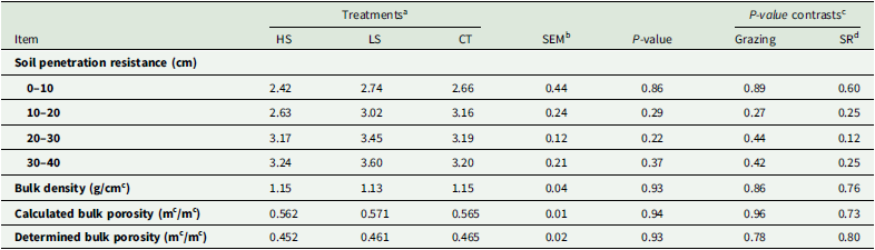
The PR data are presented in Table 2. No grazing or stocking rate effects were detected (P ≥ 0.22) for PR in the four depths evaluated.
Effects of grazing and stocking rate on physical analysis of the soil penetration resistance, bulk density, and bulk porosity of the snaplage residue

Table 2. Long description
The table presents data on soil penetration resistance, bulk density, and bulk porosity under different treatments. It has 4 rows and 8 columns. The columns are labeled as Item, HS, LS, CT, SEM, P-value, Grazing, and SR. The rows are labeled with different items: Soil penetration resistance (cm) at depths 0-10, 10-20, 20-30, and 30-40; Bulk density (g/cm^3); Calculated bulk porosity (m^3/m^3); and Determined bulk porosity (m^3/m^3). The values for each treatment (HS, LS, CT) and their corresponding standard errors (SEM) and P-values are listed. Notable trends include variations in soil penetration resistance at different depths and consistent bulk density values across treatments.
a Treatments: HS (High stocking rate; 7.0 AU/ha), LS (Low stocking rate; 3.5 AU/ha), CT (Ungrazed control).
b SEM: Standard error of means.
c Contrasts: Grazing (CT versus HS + LS), Stocking rate (HS versus LS).
d SR = Stocking rate.
Soil chemical analyses
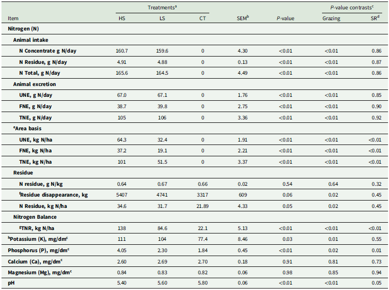
The nitrogen (N) variables are presented in Table 3. The UNE, FNE and total N excretion were increased with grazing (P < 0.01). However, N variables were not affected by stocking rate (P ≥ 0.85). There were grazing effects (P < 0.01) for UNE total (kg/ha), FNE (kg/ha) and animal N excretion total (kg/ha). There were also differences in stocking rate (P < 0.01) with HS having 50% more excretion than LS per ha. There was an effect of grazing (P = 0.02) for N return via residue. Grazing increased return by 37% compared to the ungrazed treatment. However, there were no differences (P = 0.45) between stocking rates. The total nitrogen balance increased due to grazing (82% compared to ungrazed; P < 0.01). In addition, a stocking rate effect was observed (LS < HS; P = 0.01), with HS having 40% more N returned than LS.
Effects of grazing and stocking rate on nitrogen balance and soil chemical analysis at a depth of 0 – 20 cm of the snaplage residue

Table 3. Long description
The table presents data on nitrogen variables and soil chemical analysis under different treatments. It has 18 rows and 8 columns. The columns are labeled as Item, Treatments (HS, LS, CT), SEM, P-value, and P-value contrasts (Grazing, SR). The rows are labeled with various nitrogen variables and soil chemical analysis metrics. Each row provides values for HS, LS, CT treatments, SEM, P-value, and P-value contrasts for Grazing and SR. The table includes data on animal intake, animal excretion, area basis, residue, nitrogen balance, and soil chemical analysis. Notable trends include increased UNE, FNE, and total N excretion with grazing, and differences in stocking rate with HS having 50% more excretion than LS per ha. Grazing also increased N return via residue and total nitrogen balance.
a Treatments: HS (High stocking rate; 7.0 AU/ha), LS (Low stocking rate; 3.5 AU/ha), CT (Ungrazed control).
b SEM: standard error of the means.
c Contrasts: grazing (CT vs. HS + LS) and stocking rate (HS vs. LS).
d SR = stocking rate.
e Area basis: Values were calculated based on paddock area and number of animals per paddock and are expressed on a per-hectare basis.
f Residue disappearance excludes the portion consumed by animals.
g TNR = total nitrogen returned (animal N + residue N).
h For more soil details, see Lima et al. (Reference Lima, Cruz, Borges, Gionbelli, Ladeira, Shike, Casagrande and Bernardes2024).
FNE, faeces nitrogen excretion; TNE, Total nitrogen excretion; TNR, Total nitrogen returned; UNE, urinary nitrogen excretion.
The macronutrients P and K also increased with grazing. The concentration of K, averaged across grazed treatments (HS and LS), increased by 28% compared to the ungrazed control (107 vs. 77.4 mg/dm3). However, the K concentration was not affected by the stocking rate (P = 0.55). The P concentration increased (P = 0.02) 72% with grazing. Additionally, HS increased (P = 0.01) P concentration by 43% compared to LS. Grazing resulted in a decrease (P < 0.01) in pH compared to ungrazed (5.5 vs. 5.8). Furthermore, a stocking rate effect (P = 0.05) was observed. The LS pH was 4% greater than HS (5.6 vs 5.4). The calcium (Ca) and magnesium (Mg) concentrations were no different (P ≥ 0.73) within grazing and the stocking rates evaluated.
Subsequent crop yield
Grazing positively affected all parameters of productivity of the subsequent crop that were evaluated (Table 4). The total yield mass, vegetative components mass and ear mass increased by grazing, that is, 15, 17 and 13%, respectively, compared to ungrazed (P < 0.04). However, there were no differences (P ≥ 0.83) between stocking rates.
Effects of grazing and stocking rate on total mass yield, vegetative components mass, ear in the subsequent corn crop

Table 4. Long description
A table with four rows and six columns comparing the effects of grazing and stocking rate on total mass yield, vegetative components mass, and ear mass in the subsequent corn crop. The columns are labeled Item, Treatments, SEM, P-value, and P-value contrasts. The Treatments column has sub-columns labeled HS, LS, CT, and SEM. The P-value contrasts column has sub-columns labeled Grazing and SR. Row 1: Total mass yield (kg of DM/ha), HS 33,180, LS 32,910, CT 28,160, SEM 1.73, P-value 0.09, Grazing 0.03, SR 0.91. Row 2: Vegetative C. mass (kg of DM/ha), HS 10,780, LS 10,850, CT 8,970, SEM 0.61, P-value 0.07, Grazing 0.02, SR 0.93. Row 3: Ear mass (kg of DM/ha), HS 22,410, LS 22,070, CT 19,360, SEM 1.13, P-value 0.11, Grazing 0.04, SR 0.83.
a Treatments: HS (High stocking rate; 7.0 AU/ha), LS (Low stocking rate; 3.5 AU/ha), CT (Ungrazed control).
b SEM: Standard error of the means.
c Contrasts: Grazing (CT versus HS + LS), Stocking rate (HS versus LS).
d SR = Stocking rate.
Relationship among response variables
The PC1 and PC2 explained 29.4 and 23.6%, respectively, of the variability in the dataset (Figure 4). The higher values of residue mass (RM) and pH are associated with the treatment without grazing (CT). The data for animal N, residue N and P were more associated with the HS treatment, indicating higher values for these attributes. The data of total yield of dry matter, vegetative components mass and ear mass, although closer to the high stocking rate treatment, were also associated with low stocking rate, showing that grazing was sufficient to increase productivity. In addition, the parameters of soil density, macroporosity, PR at field capacity and weighted mean diameter were not associated with grazing.
Biplot principal components analyses High: High stocking rate; Low: low stocking rate; Ungrazed: ungrazed control; RM: residual mass; SD: soil density; MACROp: macroporosity; PRfc: penetration resistance at field capacity; WMD: weighted mean diameter; pH: soil pH; P: phosphorus; K: potassium; AN: animal nitrogen; RN: residue nitrogen; SB: sum of bases, T: cation exchange capacity; V: soil base saturation; TYdm: total yield dry matter; MVC: mass of vegetative components; EM: ear mass.

Discussion
The overall effectiveness of the ICLS is improved through advances in each sector. Improvements related to the soil’s physical, chemical and biological properties and the breaking of biotic cycles (pests, diseases) contribute to increasing the system’s productivity. This can lead to increased productivity of grain, meat or milk and has the potential to reduce production costs with less use of agrochemicals and reduced use of fertilizers. Due to their intricate connection, it is not easy to analyse the effect of each component individually (Balbino et al., Reference Balbino, Vilela, Adriano, Cordeiro, de Oliveira, Pulrolnik, Kluthcouski, Luís and da Silva2012). In the current study, each factor involved will be discussed separately showing the interrelationships and impacts on subsequent crop yield.
The first factor is residue removal. In high yielding crops, large amounts of residue often remain in the field and residue management may influence subsequent crop performance (Karlen et al., Reference Karlen, Birrell, Johnson, Osborne, Schumacher, Varvel, Ferguson, Novak, Fredrick, Baker, Lamb, Adler, Roth and Nafziger2014). Karlen et al. (Reference Karlen, Birrell, Johnson, Osborne, Schumacher, Varvel, Ferguson, Novak, Fredrick, Baker, Lamb, Adler, Roth and Nafziger2014) reported that removal of 46 to 85% of corn residue, defined as moderate and high removal, respectively, increased corn yield in 57 and 51% of the evaluated sites. In this experiment, residue was reduced by 58% under grazing treatments, including both animal removal and weathering, compared to a 40% reduction in the ungrazed control (CT). Therefore, residue removal through grazing in the present study was within the range reported by Karlen et al. (Reference Karlen, Birrell, Johnson, Osborne, Schumacher, Varvel, Ferguson, Novak, Fredrick, Baker, Lamb, Adler, Roth and Nafziger2014) and is consistent with conditions associated with increased subsequent corn yield. This response may be related to the mitigation of residue-related constraints, such as nitrogen immobilization and reduced soil temperature, as suggested by Karlen et al. (Reference Karlen, Birrell, Johnson, Osborne, Schumacher, Varvel, Ferguson, Novak, Fredrick, Baker, Lamb, Adler, Roth and Nafziger2014). The similarity in initial residue mass among treatments can be explained by the fact that the same area was used, under the same conditions and only divided into paddocks. The climatic conditions favour the disappearance of the residue (Lehman et al., Reference Lehman, Ewing, Liu, Villamil, Rodriguez, Green-Miller and Shike2021). The weather conditions are the primary factor that accelerates the process of deterioration of the residue in the field. It is noted in Figure 1 that the amount of rainfall was above average during the first weeks of the experimental period, and furthermore, intake and trampling increased the residue disappearance in grazing treatments (Lehman et al., Reference Lehman, Ewing, Liu, Villamil, Rodriguez, Green-Miller and Shike2021; Parr and Papendick, Reference Parr, Papendick and Oschwald2015; Ward, Reference Ward1978). The residue intake is characterized by selectivity, as the animals search for the more digestible components such as leaves and husks. Consequently, this search likely increases trampling (Fernandez-Rivera and Klopfenstein, Reference Fernandez-Rivera and Klopfenstein1989; Gutierrez-Ornelas and Klopfenstein, Reference Gutierrez-Ornelas and Klopfenstein1991; Lehman et al., Reference Lehman, Ewing, Liu, Villamil, Rodriguez, Green-Miller and Shike2021; Stalker et al., Reference Stalker, Blanco-Canqui, Gigax, McGee, Shaver and van Donk2015). Thus, when using high stocking rates, this effect is amplified. From the end of the experimental grazing period until the beginning of the subsequent crop planting, residue mass continued to decrease (Figure 3b), reflecting ongoing degradation processes (Lamm and Ward, Reference Lamm and Ward1981). However, residue disappearance was greater in grazed treatments, with a 30% reduction in pre-planting mass relative to the final mass, compared to an 18% reduction in the ungrazed control (CT). This indicates that grazing accelerated residue breakdown beyond that driven by natural weathering alone. Trampling likely contributed to this effect by increasing residue fragmentation and surface exposure, enhancing microbial activity and decomposition rates (Rakkar and Blanco-Canqui, Reference Rakkar and Blanco-Canqui2018a). The magnitude of residue reduction observed in this study is within the range reported for grazed crop residue systems, where animal activity has been shown to accelerate residue turnover and nutrient cycling (Rakkar and Blanco-Canqui, Reference Rakkar and Blanco-Canqui2018a; Lehman et al., Reference Lehman, Ewing, Liu, Villamil, Rodriguez, Green-Miller and Shike2021). From a management perspective, this accelerated residue decomposition may enhance short-term nutrient availability; however, it may also reduce soil surface cover, which can have implications for soil protection depending on environmental conditions and residue levels.
The HS reduced weeds in the area (Figure 3c) due to the high density that intensified trampling and grazing (Sulc and Tracy, Reference Sulc and Tracy2007) and may have decreased the seed bank of these weeds. This response was observed by Reintam and Kuht (Reference Reintam, Kuht and Price2012), who reported a reduction in the seed bank in barley fields due to trampling by animals. The weeds are trampled and killed by the animals during germination and development, thus reducing their prevalence. The current experiment observed a 27% reduction in weeds when comparing the grazing to ungrazed treatment. Also, increasing stocking rate reduced weed incidence by 53%. Similar mechanisms may be a factor when analysing the appearance of grass in the area (Figure 3d). Depending on the objective of the production system, grass in crop fields is often viewed as a weed since its presence can negatively affect the main crop. In the current experiment, the incidence of grass was affected by both grazing and between stocking rates. This is explained by animals grazing and trampling these plants when they emerge, thus preventing their development. Without animal interference in the ungrazed treatment, these plants continued to grow. Grazing and increasing the stocking rate is a strategy to control weeds in the planting area of the subsequent crop, thus reducing the cost and need of herbicides to control weeds.
The effect of grazing crop residues on soil properties is a major concern of farmers when adopting ICLS since the presence of animals has been reported to increase or promote soil compaction. Our results showed no effect on the soil physical characteristics of bulk density and soil PR, comparing the grazed with ungrazed treatments. Soil density values above 1.47 Mg m−3 for clay soils and 1.80 Mg m−3 for sandy soils limit root growth (USDA, 2022). Thus, the values observed in the current experiment were below the values that would limit root growth. For Brazilian soils, based on the findings of Reichert et al. (Reference Reichert, Reinert and Braida2003) the critical soil density ranges from 1.30 to 1.40 Mg m−3 for clayey soils, 1.40 to 1.50 Mg m−3 for clayey loamy soils and 1.70 to 1.80 Mg m−3 for sandy loam soils. In the current experiment, the values averaged 1.14 Mg m−3. The PR was not affected (Table 2), and similarity between grazed and ungrazed treatments was observed. Cattle have great compaction power depending on their age and weight, with a pressure that varies from 98 to 192 kPa (Taboada et al., Reference Taboada, Lavado, Svartz and Segat1999), whereas a tractor has an average of 27 to 68 kPa (Rakkar and Blanco-Canqui, Reference Rakkar and Blanco-Canqui2018a). In the current experiment, the PR data showed that there was no compaction in the evaluated treatments, especially in the 0–10 cm layer, where any compaction by grazing animals can occur (Bell et al., Reference Bell, Kirkegaard, Swan, Hunt, Huth and Fettell2011; Greenwood and McKenzie, Reference Greenwood and McKenzie2001). However, the treatments evaluated had an average of 2.60 MPa. This value is lower than that of Moraes et al. (Reference Moraes, Debiasi, Carlesso, Franchini and Silva2014), who consider values above 3 and 3.5 Mpa for minimum tillage and no-till, respectively, to characterize compaction.
No effect on soil physical characteristics may be explained by the stocking rates used, season of the year and the possible positive effect on soil aggregates. In the current experiment, the HS treatment (7.0 AU (500 kg)/ha or 8.3 AU (450 kg)/ha) was below the minimum that is considered to cause any damage to soil aggregates, which is 9.3–13 AU (450 kg)/ha (Rakkar et al., Reference Rakkar, Blanco-Canqui, Drijber, Drewnoski, MacDonald and Klopfenstein2017). Cattle faeces can increase the concentration of organic matter in soil (Maillard and Angers, Reference Maillard and Angers2014; Schlegel et al., Reference Schlegel, Assefa, Bond, Wetter and Stone2015). Due to having about half the density of mineral soil particles, organic matter can increase the elasticity of the soil matrix (Blanco-Canqui et al., Reference Blanco-Canqui, Hergert and Nielsen2015; Soane, Reference Soane1990). Thus, grazing did not affect soil physical characteristics. In the present study, the grazing period occurred during the dry season, characterized by low rainfall and reduced soil moisture, which likely increased soil load-bearing capacity and reduced susceptibility to compaction (Rakkar and Blanco-Canqui, Reference Rakkar and Blanco-Canqui2018a).
Snaplage residue grazing increased N, C and mineral levels in the soil through animal faeces and urine when animals were supplemented (Drewnoski et al., Reference Drewnoski, MacDonald, Erickson, Hanford and Klopfenstein2016; Maughan et al., Reference Maughan, Flores, Anghinoni, Bollero, Fernández and Tracy2009). In the current experiment, grazing increased N concentrations compared to the ungrazed treatment. High-stocking rate and LS treatments added an equivalent of 100 and 50 kg of N/ha respectively, only from the animal. In addition to this, an increase in the N return by residue decomposition post-grazing was observed for previously mentioned factors. The increase in N may have been one of the factors that contributed to subsequent yield increase. Studies indicate that adding N leads to increased grain yield by affecting grain weight, the number of kernels per ear, ear weight and protein concentration (Wei et al., Reference Wei, Wang, Li, Qin, Jiang and Dong2019). In Brazil, when farmers want to increase yield, nitrogen application is a widely used technique because Brazilian soils have low N content and consequently a high C:N ratio. This is especially true when there are crop residues in the soil, which have a C:N ratio ranging from 26 to 82:1 (Rakkar and Blanco-Canqui, Reference Rakkar and Blanco-Canqui2018a).
Grazing in addition to concentrated feed increased the input of K and P in the cropping system. Although the removal of these nutrients is greater with grazing residue by animals, a large amount of these nutrients returns to the system via faeces (Rakkar et al., Reference Rakkar, Blanco-Canqui, Drijber, Drewnoski, MacDonald and Klopfenstein2017). However, many places have concerns about the levels of P in the soil mainly when applied in large quantities (Hilimire, Reference Hilimire2011; Russelle et al., Reference Russelle, Entz and Franzluebbers2007). In Brazil, most soils are poor in P and K, thus, increasing the content of these nutrients using integration can be an essential tool to increase productivity as shown in the data of the current experiment.
The difference in soil pH with grazing can be explained by the deposition of faeces and urine by the animals, which was higher in the HS treatment when compared to the LS. The decomposition of the organic matter present in the excreta by soil microorganism’s releases ammonia (NH3) which turns to nitrate releasing H+. One of the processes of soil acidification is the accumulation of organic matter and a consequent increase in CEC and acidity exchange (Haynes, Reference Haynes1983). The urea present in the animal’s urine releases H + by reacting the NH4 with the soil. H + ions in the soil, in turn, favour soil acidification (Meurer et al., Reference Meurer, Bissani, Carmona and Meurer2010). Although the decrease in pH content is statistically different, the difference was insufficient to cause any agronomic impact on the subsequent crop due to the proximity of the values. In the current experiment, the addition of animals to the system increased the subsequent crop yield (Table 4).
Grazing affected parameters cited above such as nutrient return and residue removal that impact yield increase. However, increasing the stocking rate did not affect subsequent yield, although an increase in the parameters cited was observed in HS when compared to LS. The vegetative components and ear mass followed the same pattern as the total yield mass when comparing the grazing or stocking rate evaluated. Similar to Lima et al. (Reference Lima, Bastos, Ávila, Ferreira, Casagrande and Bernardes2022), There was a high correlation between these two components with total dry matter production, being a good marker of productivity.
The productivity increase in crop and animal components in ICLS systems results from the interaction of several factors and is often difficult to separate. The factors that positively affect production are positively correlated with grazing. Among these factors, the return of macronutrients such as N and P increased when the residue was grazed, and this increase was positively correlated with yield parameters, independent of the stocking rate evaluated. A positive correlation among stocking rate, animal nitrogen, residue N, K, P, total yield of dry matter, mass of vegetative components and ear mass suggests that the presence of animals grazing the residue increases the subsequent crop yield. Also, this may indicate a high correlation with the increase in the stocking rate.
The other soil parameters involved in the analysis were not correlated with the evaluated treatments. The lack of correlation between grazing and these parameters suggests they did not affect subsequent production. In addition, only the RM and pH were related to the non-grazed treatment.
In ICLS aimed at optimizing land use, the reduction of inorganic fertilizer may be an economical strategy to reduce input costs. Although it has some nutrients, animal excreta cannot reach the amount of nutrients that a crop needs, either because of low density (Gupta et al., Reference Gupta, Rai and Risam2012) or because of its localized application. Based on the results of the current experiment, an alternative fertilization strategy could be a combination of both sources (chemical and organic), thereby reducing fertilizer acquisition costs and potentially reducing economic inputs.
The use of residue grazing in the current experiment has proven to be an excellent tool, since it was possible to integrate two corn crops with beef cattle finishing, maximizing the use of land during the fallow period between crops. In several places, there are reports of income increases with the use of ICLS, reducing the vulnerability of these production systems to climatic or market events (Peyraud et al., Reference Peyraud, Taboada and Delaby2014; Russelle et al., Reference Russelle, Entz and Franzluebbers2007). Moreover, the reduction in production costs through complementarities between crop and livestock, such as possible reduction in the amount of fertilizer and herbicides, decreases dependence on factors beyond the control of the producer. It is important to note that the results of this study are based on a single grazing cycle and, therefore, represent short-term responses. Long-term and cumulative effects, such as potential soil compaction and changes in nutrient dynamics, may require multiple grazing cycles to be fully understood.
Conclusion
The use of the snaplage residue for cattle finishing is a viable strategy utilized in the ICLS. Grazing residue had no short-term negative effects on the physical characteristics of the soil while increasing concentrations of macronutrients such as nitrogen and phosphorus from animal supplementation. These data indicate that grazing residue positively affected subsequent corn yield, regardless of the stocking rate used. Grazing snaplage residue as a roughage source enabled the addition of beef production between two corn crops without negatively affecting production of the crop following grazing. However, further research is required to validate these findings over multiple years.
Data availability
Data will be made available on request.
Acknowledgements
The authors thank the members of NEFOR (Brazilian Forage Team) for their contributions during the field trial setup.
Author contributions
IBGL, TFB and DRC conceived and designed the study. IBGL, TFB, JJMSF, BGCH, BMS, PJRC and DWS conducted the investigation and contributed to data gathering. JJMSF, BGCH, BMS and PJRC performed data curation and formal analyses. IBGL, TFB and DRC wrote the original draft. All authors contributed to writing, reviewing and editing the manuscript. TFB and DRC acquired funding.
Funding statement
This work was funded by the National Council for Scientific and Technological Development (CNPq), National Institute of Science and Technology in Animal Science (INCT-CA), the Minas Gerais Research Foundation (FAPEMIG) and Coordination for the Improvement of Higher Education Personnel (CAPES).
Competing interests
The authors declare no conflicts of interest.
Ethical standards
All the experimental procedures of this study were approved by the Ethics and Animal Welfare Committee of the Federal University of Lavras (protocol number 008/2019).






 Open access

