2.1 Computational methods

An orthogonal curvilinear grid solver, CFDShip-Iowa Version 6.2 (Suh, Yang & Stern Reference Suh, Yang and Stern2011; Wang et al. Reference Wang, Suh, Yang and Stern2012b ), is used for the computations. This solver was extended from the Cartesian grid solver (version 6.1) (Yang & Stern Reference Yang and Stern2009; Wang et al. Reference Wang, Yang, Koo and Stern2009a ; Wang, Yang & Stern Reference Wang, Yang and Stern2009b ) for two-phase incompressible viscous flows with the state-of-the-art numerical methods recently developed at the University of Iowa. In this solver, both gas and liquid phases are considered for the strong interactions between two phases. The level-set-based ghost fluid method is adopted for sharp interface treatment and the volume-of-fluid (VOF) method is used for the interface tracking. A brief description of the numerical methods are given below, and details can be found in the papers given herein.

A finite difference method is used to discretize the Navier–Stokes equations on a non-uniform staggered orthogonal grid. Time advancement of the present study is based on the semi-implicit four-step fractional step method (Choi & Moin Reference Choi and Moin1994). The diagonal diffusion terms are advanced with the second-order Crank–Nicholson method and the other terms by the second-order explicit Adams–Bashforth method. The convective terms are discretized using third-order QUICK (Leonard Reference Leonard1979) and fifth-order WENO (Jiang & Shu Reference Jiang and Shu1996) schemes. Semi-Lagrangian advection schemes for the Navier–Stokes equations are also implemented to increase the maximum allowable time step. All other terms are discretized with the standard second-order central difference scheme. The pressure Poisson equation is solved using the HYPRE library (Falgout, Jones & Yang Reference Falgout, Jones, Yang, Bruaset and Tveito2006).

An accurate and robust new VOF method developed by Wang, Yang & Stern (Reference Wang, Yang and Stern2012c ) is used to solve the VOF advection equations. The interface normal vector is evaluated using a signed distance function obtained from a second-order distance function construction scheme. A novel technique for the calculation of the normal vector is developed, which is very robust and accurate, especially for the under-resolved regions. A semi-Lagrangian advection scheme for the VOF method (Wang, Yang & Stern Reference Wang, Yang and Stern2012d ) is used to eliminate the time step constraints due to the CFL condition and to speed up the computations. As a combined Eulerian and Lagrangian method, the semi-Lagrangian method is unconditionally stable and also maintains the efficiency of the Eulerian method.

The code parallelization is done via a domain decomposition technique using the MPI library. A simple domain decomposition technique is used in all three directions which facilitates the use of thousands of processors, even with coarse grids. Parallel I/O using MPI2 have been implemented (Yang et al. Reference Yang, Bhushan, Suh, Wang, Koo, Sakamoto and Xing2008) such that all processors read from and write to one single file simultaneously, which is much more effective than one or a few processors receiving data from all processors and writing to one or a few files. This is critical for simulations using billions of grid points since the memory of a few processors is insufficient to handle such huge data sets. Numerous numerical tests and application examples have been performed to verify and validate the code such as a static drop in equilibrium for surface tension modelling, a small-scale single bubble rising in quiescent water, droplet impact onto a liquid pool and plunging wave breaking (Yang & Stern Reference Yang and Stern2007, Reference Yang and Stern2009; Wang et al. Reference Wang, Yang, Koo and Stern2009a ,Reference Wang, Yang and Stern b ; Suh et al. Reference Suh, Yang and Stern2011; Koo et al. Reference Koo, Wang, Yang and Stern2012; Wang et al. Reference Wang, Yang and Stern2012a –Reference Wang, Yang and Stern d ). The accuracy, robustness and efficiency of the numerical methods especially for interface tracking, sharp interface treatment and surface tension modelling have been extensively verified.

2.2 Computational set-up

The computational conditions and physical parameters are similar to those used in the 2-D studies by Chen et al. (Reference Chen, Kharif, Zaleski and Li1999), Iafrati (Reference Iafrati2009, Reference Iafrati2010) and Wang et al. (Reference Wang, Yang, Koo and Stern2009a ). The wave profile is initialized using the following function

where ${\it\epsilon}=0.55$ is the wave slope. The wavelength ${\it\lambda}$ is used as the reference length and the reference velocity is chosen as $U_{r}=\sqrt{g{\it\lambda}}$ . The Weber number is $We={\it\lambda}\sqrt{g{\it\rho}_{w}/{\it\sigma}}=100$ and the Reynolds number is $Re={\it\rho}_{w}g^{1/2}{\it\lambda}^{3/2}/{\it\mu}_{w}\simeq 4.4\times 10^{5}$ , where $g$ is the gravity accceleration, ${\it\rho}_{w}$ is the water density, ${\it\sigma}$ is the surface tension coefficient and ${\it\mu}_{w}$ is the water viscosity, which correspond to a water wave with a wavelength of 27 cm.

Three different grids were used for the computations with a minimum grid spacing of 0.264 mm, 0.132 mm and 0.065 mm (see table 1), respectively. The computations for the coarse and medium grids were carried out in a 3-D domain of [ $-0.5{\it\lambda}$ , $0.5{\it\lambda}$ ], [0, $0.5{\it\lambda}$ ] and [ $-0.5{\it\lambda}$ , $0.5{\it\lambda}$ ] in the streamwise, spanwise and vertical directions, respectively. For the fine grid case, the spanwise dimension was reduced to $[0,0.25{\it\lambda}]$ in order to save computational resources. Uniform grid spacing was used in the streamwise and spanwise directions. In the vertical direction, uniform grid spacing was used for $-0.25{\it\lambda}<z<0.25{\it\lambda}$ and the grid spacing gradually increased below $z=-0.25{\it\lambda}$ and above $z=0.25{\it\lambda}$ . Periodic boundary conditions were imposed in both streamwise and spanwise directions and the slip boundary conditions were applied in the vertical direction. Constant time steps were used for the three grids as shown in table 1. The time was non-dimensionalized by $t_{r}=\sqrt{{\it\lambda}/g}$ . The simulations were started at time $t=0.0$ with the velocity in the liquid phase initialized using the velocity potential and the air phase at rest. For the fine grid, the 2-D results (wave profile and velocity field before plunging) were used as the initial conditions.

There are many challenges and difficulties for simulations using huge grid sizes (billions of grid points), such as data transfer and storage, data visualization, analysis and animation. In the present study, a high priority queue was requested and approved by the US DoD Supercomputing Resource Centers (DSRC) with 4 and 11.2 million CPU hours for FY2013 and FY2014, respectively. This is critical to obtain enough processors and avoid unacceptable waiting time in the queue to speed up the computations, and also to facilitate data post-processing using HPC job based software in parallel mode.

Computational results for the overturning jet before wave plunging on the three grids are shown in figure 1 for grid convergence studies. Similar grid studies for the wave breaking simulations can be found in Wang et al. (Reference Wang, Yang, Koo and Stern2009a ) and Brucker et al. (Reference Brucker, O’Shea, Dommermuth and Adams2010). The overall structures of the interface obtained on the three grids are similar. The jet tip is slightly thinner and sharper on a fine grid than on a coarse grid since a fine grid can capture more details of the interface structure. The relative errors of the interface location are evaluated by using the $L_{1}$ norm (Wang et al. Reference Wang, Yang and Stern2009b ), as shown in table 2. As shown in the table, the relative error decreases with grid refinement, which indicates the convergence of the computational results. As discussed in Chen et al. (Reference Chen, Kharif, Zaleski and Li1999) and Lubin et al. (Reference Lubin, Vincent, Abadie and Caltagirone2006), grid convergence analysis is quite difficult for this kind of flow which is characterized by unsteady air–water interface breaking. Although smaller interface structures can be resolved with higher grid resolution, the overall flow dynamics of wave breaking is not much affected by the small interface structures. The results computed on the medium grid are used for the following discussions unless otherwise stated.

Figure 1.

Comparison of the wave profiles of the three different grids at $t=1.25$ : coarse grid (solid line), medium grid (dashed line) and fine grid (dash-dotted line). $h$ is the height of wave breaking region, which will be used to calculate the energy dissipation rate in § 3.4.

Table 1.

Simulation configurations for the coarse, medium and fine grids.

Table 2.

Relative errors of the interface location between the consecutively reduced grid spacing at $t=1.25$ .

The kinetic ( $E_{k}$ ), potential ( $E_{p}$ ) and total ( $E_{t}$ ) energies of the wave breaking are evaluated according to the formulations given in Chen et al. (Reference Chen, Kharif, Zaleski and Li1999) and Iafrati (Reference Iafrati2009). The time histories of the kinetic, potential and total energy for the coarse and medium grids are shown in figure 2 along with the 2-D computational results by Chen et al. (Reference Chen, Kharif, Zaleski and Li1999). The results are non-dimensionalized using their initial values and the time is non-dimensionalized using the time scale given above. As shown in the figure, the present simulation results for the two grids are almost identical at the early wave breaking stage. After approximately $t=1.5$ , fluctuations can be observed in the kinetic energy, whereas both the total and potential energies are still very close. As compared to the results by Chen et al. (Reference Chen, Kharif, Zaleski and Li1999), the energy time histories exhibit similar trends. The kinetic energy in the present simulations shows a higher jump after jet plunges, which can also be found in the results of Lubin et al. (Reference Lubin, Vincent, Abadie and Caltagirone2006). The total energy of the present simulations is also higher than that of Chen et al. (Reference Chen, Kharif, Zaleski and Li1999) and slightly rises before plunging. A similar trend can be found in figure 16 of Lubin & Glockner (Reference Lubin and Glockner2015). This is because the Reynolds number used in the present study is much larger than that used in Chen et al. (Reference Chen, Kharif, Zaleski and Li1999). Besides the higher Reynolds number, some other effects, such as the larger viscosity and density ratios (water/air), 3-D computation, much finer grid and higher-order convection schemes, are also responsible for the differences. As for the potential energy, the present simulation results are very close to Chen et al. (Reference Chen, Kharif, Zaleski and Li1999) except that a bigger rise can be found when wave crest reaches the maximum height in the present simulation.

Figure 2.

Time history of total wave energy ( $E_{t}$ ), kinetic energy ( $E_{k}$ ) and potential energy ( $E_{p}$ ).

The water–air interface is extracted from the level-set function and the bubbles/droplets are identified from the VOF function. The identification of the bubbles/droplets is performed using a non-recursive neighbour searching algorithm. A multi-block identification procedure (Herrmann Reference Herrmann2010) is employed to handle bubbles/droplets shared by different blocks. The volume of each bubble or droplet is obtained from the VOF function and an equivalent spherical diameter is then calculated. A close-up view of the droplets in the breaking wave is shown in figure 3, where the minimum droplet size that is captured is less than one grid spacing. These under-resolved bubbles/droplets will not be counted due to numerical errors. The numerical errors of VOF interface reconstruction can be significant when the bubble/droplet size is comparable to the grid spacing. As noted by Li et al. (Reference Li, Arienti, Soteriou and Sussman2010), serious advection errors will be introduced when the liquid structure is less than twice the grid spacing. As shown in figure 7.3 of Clift, Grace & Webber (Reference Clift, Grace and Webber1978), when the diameter is $d<1.0$  mm, the surface tension force is dominant and the shape of bubble/droplet lies in the spherical regime. As shown in figure 3, with more than 4 computational cells (0.53 mm) per bubble/droplet diameter, the droplets/bubbles take on a spherical shape. Herein, bubbles/droplets are considered as unresolved and will not be counted when their diameters are less than 5 computational cells. It should be noted that the small under-resolved bubbles/droplets are different from the so-called ‘flotsam’ or ‘jetsam’ which are bigger in size and mainly appear in the lower-order VOF schemes and algebraic methods (Aulisa et al. Reference Aulisa, Manservisi, Scardovelli and Zaleski2003). The VOF/PLIC scheme, as used in the present study, is more accurate and does not produce the so-called ‘flotsam’ or ‘jetsam’ (Scardovelli & Zaleski Reference Scardovelli and Zaleski2003).

Figure 3.

Close-up view of the droplets in wave breaking.

3.1 Wave breaking process

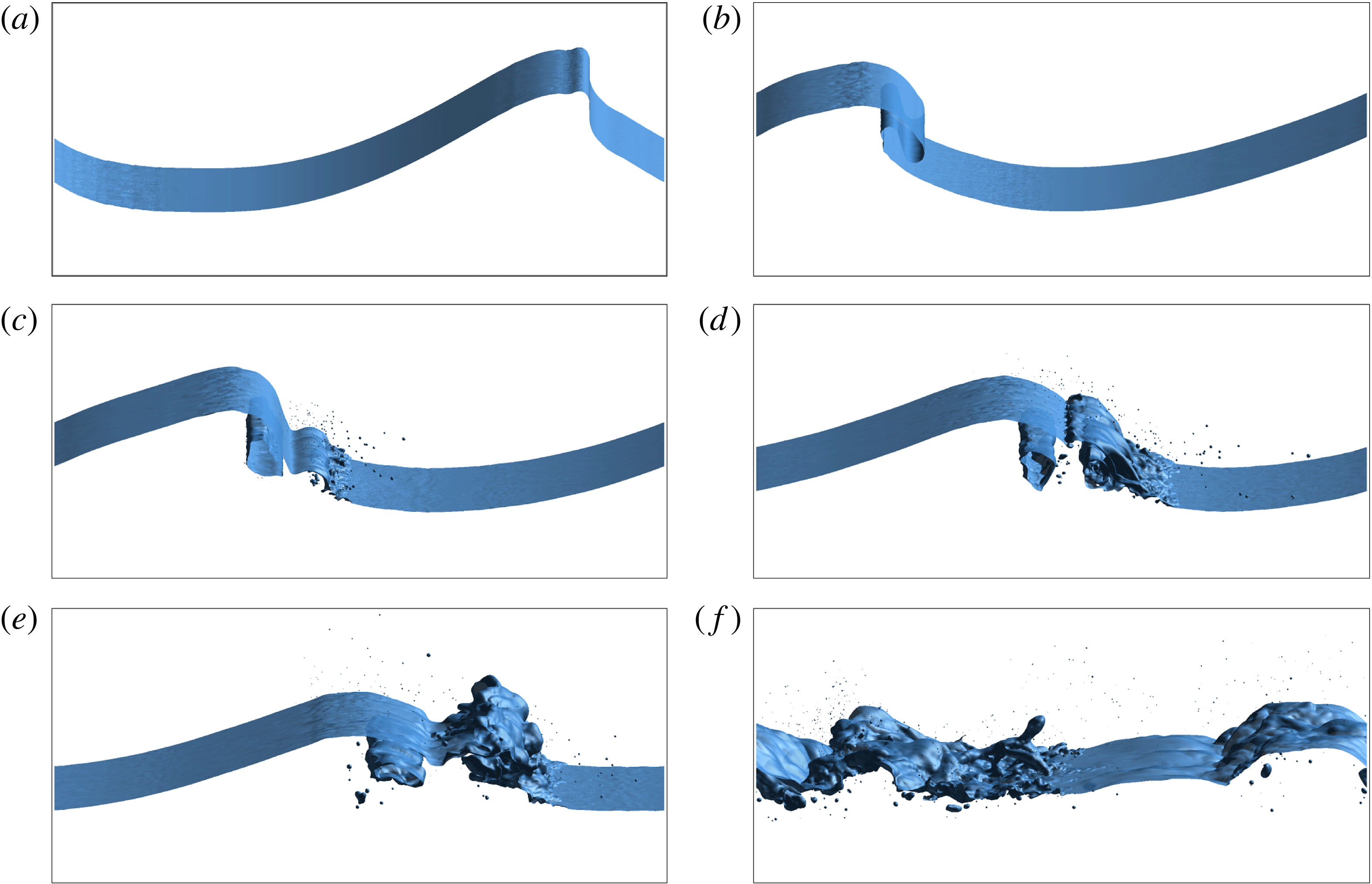
The snapshots of the time sequence of the wave breaking process are presented in figure 4. More details of the wave breaking process are shown in the supplementary movie 1 available online at http://dx.doi.org/10.1017/jfm.2016.87 with side view, perspective view and close-up view of the plunging region. The water–air interface is identified using the isosurface of the zero distance function. Droplets and bubbles are shown above and below the free surface, respectively. It is hard to tell the difference of the bubble and droplets from the figure. It is difficult to assign a different colour for water and air using the extracted isosurface to represent the interface. Different colours can be used if the phase function (distance function in present study) in the whole domain is plotted, but this is currently not feasible for the post-processing software to handle since the grid size is so large.

Figure 4.

Time sequences of Stokes wave breaking. (a) $t=0.56$ ;(b)  $t=1.20$ ; (c)  $t=1.44$ ; (d) $t=1.76$ ; (e) $t=2.08$ ; (f) $t=2.96$ . The blue surface is the air–water interface identified using the isosurface of the zero distance function, which is the same as in figures 5, 10 and 11.

The wave breaking processes shown in the figure include the formation of the maximum wave height, overturning jet, wave plunging, splash ups and subsequent wave breaking events. Figure 4(a) is for $t=0.56$ when the wave crest becomes steepest and reaches its maximum height. Figure 4(b) shows the overturning jet. The plunging jet shoots out from the wave face, falls and touches the wave trough with an air tube entrained, as shown in figure 4(c). The cross-section of the entrained air tube has a roughly elliptical shape. The plunging jet rebounds off the wave trough forming the splash ups, which subsequently grow and fan out (see figure 4 d). As the original wave crest decreases in height, a vertical jet is being formed with increased height, as shown in figure 4(e). The entrapped air tube continues to be deformed and eventually collapses and the vertical jet plunges forward after it reaches the maximum height, and the wave breaking enters the subsequent process with successive splash ups with reduced energy and chaotic flow motion. The major wave breaking events are in very good agreement with the 2-D simulations conducted by Chen et al. (Reference Chen, Kharif, Zaleski and Li1999). Detailed comparison with the results in Chen et al. (Reference Chen, Kharif, Zaleski and Li1999) for 2-D simulations has been made in the previous study by the authors (Wang et al. Reference Wang, Yang, Koo and Stern2009a ).

3.2 3-D interface structures

Figure 5 shows the wave profile at time $t=1.76$ when the splash ups are being generated after the initial jet plunges. The 3-D local interface deformation in the spanwise direction is clearly demonstrated in figure 5(b). These transient rib-like interface structures are also observed in the studies by Watanabe et al. (Reference Watanabe, Saeki and Hosking2005) and Saruwatari, Watanabe & Ingram (Reference Saruwatari, Watanabe and Ingram2009), which are related to vortex structures beneath the interface. The 3-D vortex structures are identified using the $Q$ -criterion which are shown in figure 6. $Q$ is the second invariant of the velocity gradient (Jeong & Hussain Reference Jeong and Hussain1995) and represents the balance between shear strain rate and vorticity magnitude, which is more useful to identify vortices for complicated 3-D flows than the vorticity contours. In figure 6(a), $Q$ isosurfaces are plotted for both air and water phases along with the air–water interface. It can be seen that strong organized structures with streamwise vortex filaments are wrapping around a major spanwise vortex tube in the upstream air phase. In order to show the vortex structures beneath the interface, $Q$ isosurfaces are only plotted for the water phase with the interface removed in figure 6(b). As shown in the figure, streamwise vortex filaments can be clearly found in the secondary jet (splash up). As shown in figure 7, these streamwise vortex are counter-rotating vortex pairs which can push the interface up and down and cause the interface deformation. Streamwise vortex filaments can also be seen underneath the entrained air tube in figure 6(c), which are also reported in Brucker et al. (Reference Brucker, O’Shea, Dommermuth and Adams2010) and Lubin & Glockner (Reference Lubin and Glockner2015).

Figure 5.

Wave profile of simulation at $t=1.76$ . (a) Side view; (b) front view; (c) perspective view: the dashed line shows the cross-section slice locations at $x/{\it\lambda}=-0.25$ , $-0.05$ and 0.05.

Figure 6.

3-D vortex structures of the plunging wave breaking at $t=1.76$ . (a) Perspective view of the $Q$ isosurfaces in both air and water along with the interface; (b) top view of the $Q$ isosurfaces in water phase; (c) bottom view of the $Q$ isosurfaces in water phase.

Figure 7.

Cross-section velocity vector field and vortices (secondary flow field with the subtraction of mean vertical velocity for all the locations). (a) $x/{\it\lambda}=-0.25$ ; (b) $x/{\it\lambda}=-0.05$ ; (c) $x/{\it\lambda}=0.05$ .

The analysis of the instabilities in plunging wave breaking is difficult since many complex processes and phenomena are involved. The interface deformation also depends on the combined effect of gravity, surface tension and turbulence (Brocchini & Peregrine Reference Brocchini and Peregrine2001). In an experimental study by Gui, Yoon & Stern (Reference Gui, Yoon and Stern2014a ,Reference Gui, Yoon and Stern b ), the instabilities for free-surface flow over a bump in a shallow water flume were investigated. The observed wavy gap flow exhibits jet-like velocity profiles, which is most relevant to the Görtler type centrifugal instability for convex curvature. The velocity profiles at several streamwise locations in the streamwise central plane are shown in figure 8. The detailed velocity profiles in the jet of the plunging wave breaking can be sufficiently resolved due to the high spatial resolution. According to the Görtler inviscid instability theory (Saric Reference Saric1994), a flow is stable if the velocity magnitude increases with distance away from the wall for a convex curvature. The stability criterion is $\text{d}(V_{{\it\theta}})^{2}/\text{d}r>0$ , where $r$ is the radius in the polar coordinate system with origin at the centre of curvature of the flow boundary, and $V_{{\it\theta}}$ is tangential velocity component. The Rayleigh inviscid stability requires that the angular momentum increases radially outward from the wall, i.e. the radial derivative of the circulation $(rV_{{\it\theta}})^{2}$ must increase with the radius from the centre of the curvature, $\text{d}(rV_{{\it\theta}})^{2}/\text{d}r>0$ . As shown in figures 8 and 9, in the upstream at $x/{\it\lambda}=-0.25$ , the flow is stable, whereas in the wave breaking region, the Görtler stability criterion is violated in most locations and the Rayleigh stability criterion is broken only in small regions. Therefore, the breaking wave instabilities are likely mainly due to Görtler type centrifugal instability. It should be noted that only a brief discussion of the instability analysis is given above. More detailed analysis of the wave breaking instability is out of the scope of the present paper.

Figure 8.

Velocity profiles in the jet at $y/{\it\lambda}=0.25$ . (a) Görtler inviscid instabilities; (b) Rayleigh instabilities. Red: stable; green: unstable.

Figure 9.

Intability criterion in the jet at $y/{\it\lambda}=0.25$ . (a) Görtler inviscid criterion; (b) Rayleigh inviscid criterion.

3.3 Air entrainment and spray formation

In plunging breaking waves, air can be entrained by several mechanisms, such as air tube entrapment and jet impact, entrapment by forward splash, backward-splash entrainment and turbulent entrainment, as discussed in Kiger & Duncan (Reference Kiger and Duncan2012). These air entrainment mechanisms are reproduced in the present simulation in greater detail due to the high grid resolution. Air entrainment processes are shown in figure 10 corresponding to the main air entrainment mechanisms given in Kiger & Duncan (Reference Kiger and Duncan2012). Figure 10(a–d) shows the plunging jet impact process during which an air tube is trapped. The entrapment of the air tube is the most clear and obvious air entrainment mechanism in plunging breaking waves. Air is also dragged into water when the jet hits the wave trough where very small bubbles are created at the jet impact site, as clearly shown in figure 10(a–d). Air is further entrapped as the forward splashes impact the trough surface, as shown in figure 10(e–h). Figure 10(i–l) shows the air entrainment between the backside of the rising splash and the original plunging jet. Air entrainment in the splash and turbulent wave breaking regions when the liquid ligament and droplets are formed and impact is shown in figure 10(m–p).

Figure 10.

Air entrainment process. (a–d) Jet impact; (e–h) splash impact; (i–l) backward splash; (m–p) splash and turbulent regions. Time interval between images from left to right, ${\rm\Delta}t=0.01$ for (a–h); ${\rm\Delta}t=0.02$ for (i–p).

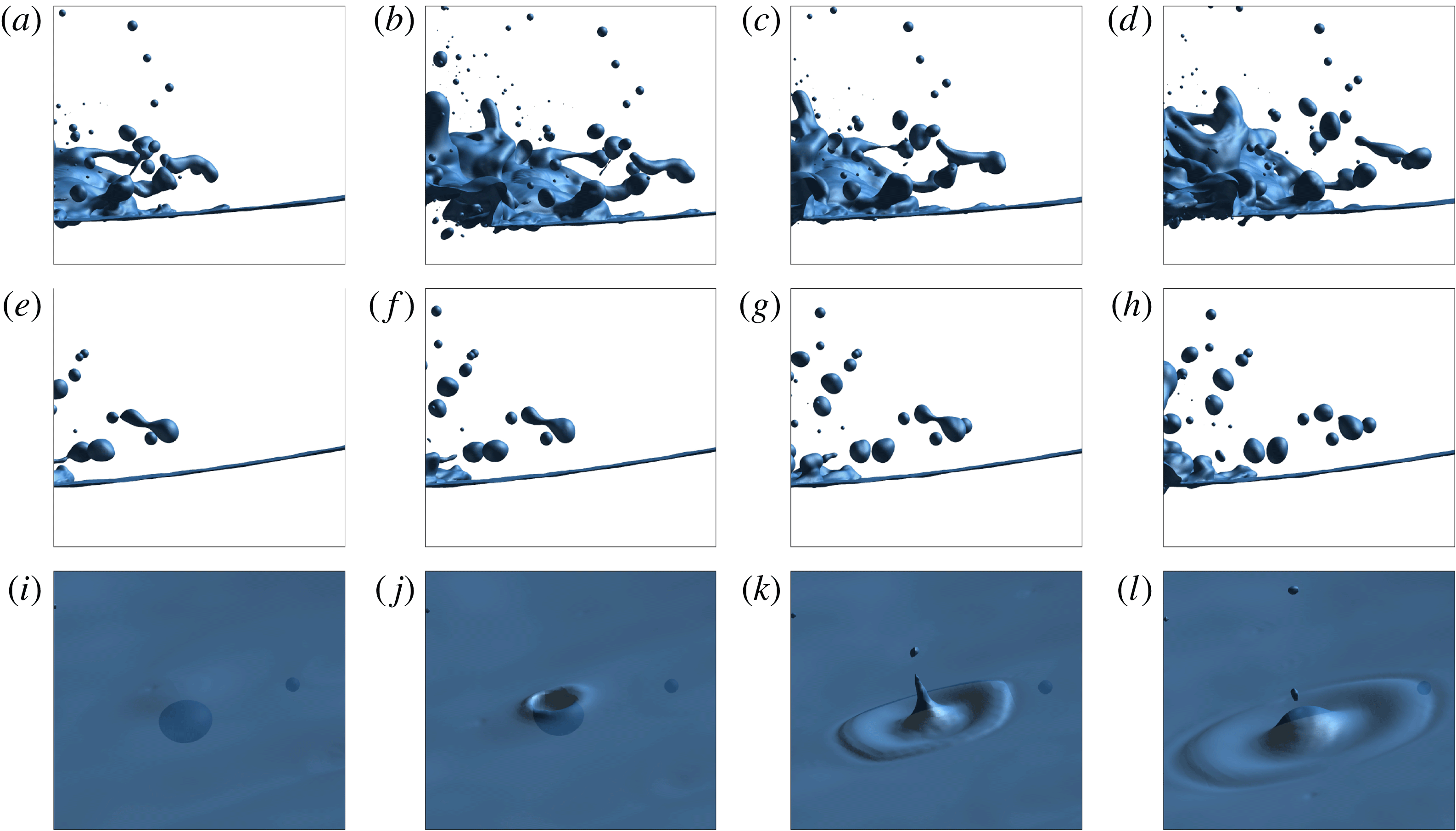
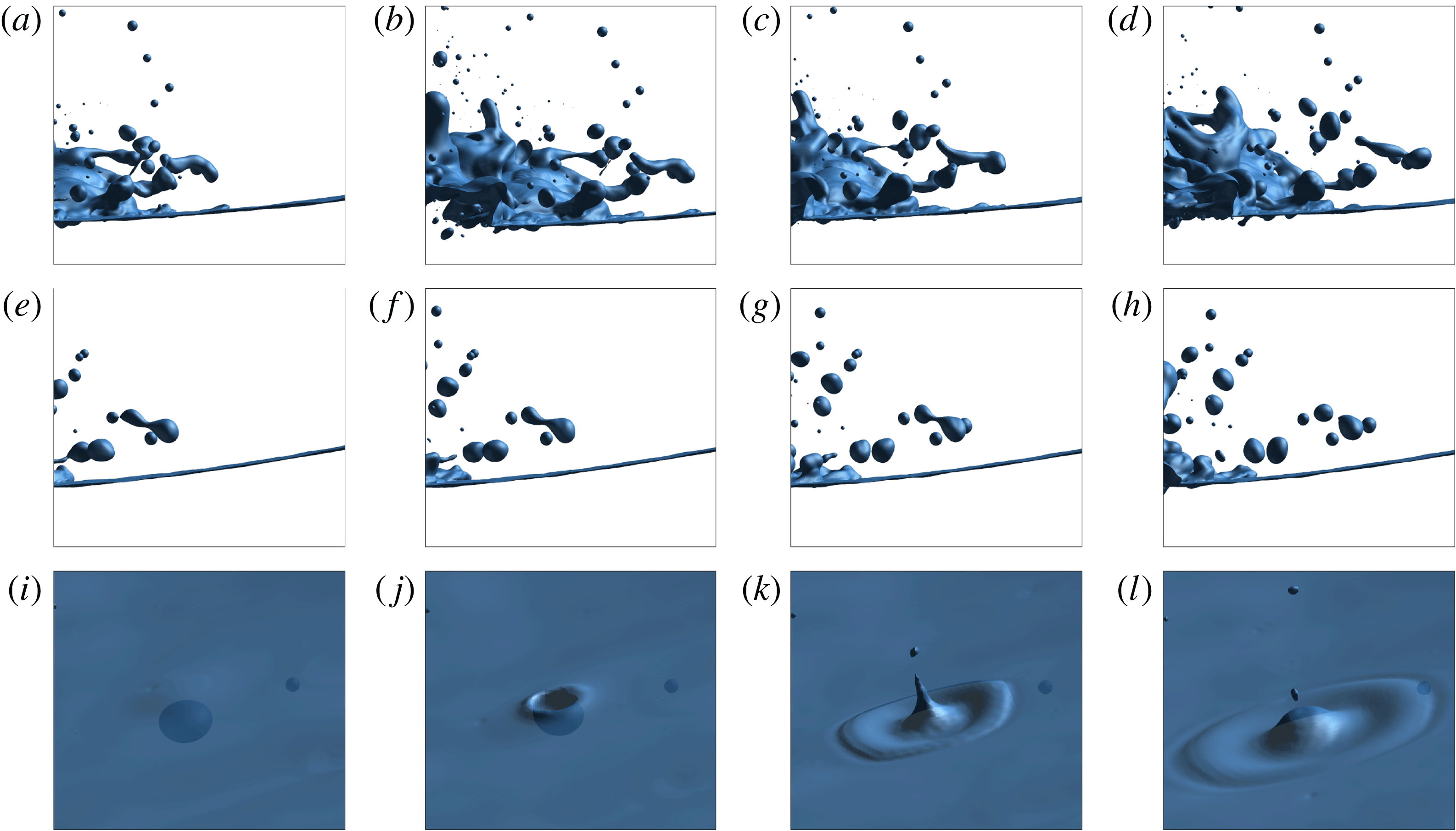
Once the jet tip touches the trough surface, splash up initiates and develops into a spray region with small droplets, as shown in figure 10(a–d). Detailed droplets and spray formation processes are given in figure 11. Figure 11(a–d) shows the liquid ligament formation and detachment from the stretched water surface. The detached ligament is then pinched off into droplets due to the surface tension effect, as shown in figure 11(e–h). This observation agrees with the spray formation mechanism explained by Longuet-Higgins (Reference Longuet-Higgins1995) for interface stretching, ligament fingering and droplet pinching off. A liquid jet is also formed and pinched off into droplets as the air bubble bursts into the air, as shown in figure 11(i–l). A detailed experimental study was conducted by Lhuissier & Villermaux (Reference Lhuissier and Villermaux2012) focusing on the spray formation of a single bubble bursting. A new spray generation mechanism was observed in the experimental study by Veron et al. (Reference Veron, Hopkins, Harrison and Mueller2012) for sea spume droplet production at high wind speed. This break-up mechanism is driven by the wind, which is not applicable in the present study.

Figure 11.

Droplets and spray formation. (a–d) Ligament detachment; (e–h) droplet break up; (i–l) bubble burst into air. Time interval between images from left to right, ${\rm\Delta}t=0.01$ for (a–h); ${\rm\Delta}t=0.02$ for (i–l).

3.4 Bubble/droplet size distribution

The experimental study by (Deane & Stokes Reference Deane and Stokes2002) found that the bubble size distribution is controlled by two distinct mechanisms. Large bubbles ( $r>1.0$ mm) are determined by turbulent fragmentation and show a $-10/3$ power-law scaling, and smaller bubbles are created by jet and drop impact and show a $-3/2$ power-law scaling. For large bubbles, turbulent fragmentation and rising-bubble fragmentation are the two possible fragmentation mechanisms in wave breaking, as discussed in Soloviev & Lukas (Reference Soloviev and Lukas2006). For turbulent fragmentation, a theoretical bubble size scaling equation was derived by Garrett, Li & Farmer (Reference Garrett, Li and Farmer2000) which correlates bubble size spectra and energy dissipation rate for bubble break ups,

where $N(r)$ is the number of bubbles per ${\rm\mu}\text{m}$ radius increment per m $^{3}$ , $Q$ is the air volume entrained per volume of water per second, ${\it\epsilon}$ is the energy dissipation rate and $r$ is bubble radius. Turbulent fragmentation will cease when the bubble radius is less than the Hinze scale ${\it\alpha}_{H}$ , which is defined as (Deane & Stokes Reference Deane and Stokes2002),

where ${\it\sigma}$ is surface tension and $We_{c}$ is the critical Weber number, which is chosen as $We_{c}=4.7$ . Bubbles smaller than the Hinze scale are stabilized by surface tension, and the process of turbulent fragmentation is believed to be less important. Deane & Stokes (Reference Deane and Stokes2002) presented a scaling equation for small bubbles following the dimensional analysis by Garrett et al. (Reference Garrett, Li and Farmer2000),

where $v$ is the jet velocity. Rising-bubble fragmentation is characterized by the rise velocity $w_{b}$ and collective interactions of rising bubbles. Soloviev & Lukas (Reference Soloviev and Lukas2006) proposed a scaling equation based on the dimensional analysis for the bubble fragmentation dominated by buoyancy forces,

The above $-3$ power law (3.4) is close to the $-10/3$ power law (3.1), and the former does not contain the energy dissipation rate ${\it\epsilon}$ .

Figure 12 shows the bubble size distributions for simulations on the three grids at different time instants along with the time averaged results. The number of bubbles is averaged over the active wave breaking period from $t=1.44$ to $t=3.25$ (total of 182 time instants) for the coarse and medium grids and from $t=1.48$ to $t=2.49$ (total of 102 time instants) for the fine grid. Simulation on the fine grid is terminated when the entrained air cavity collapses in order to save computational resources. The time average of bubble numbers is similar to those in experimental studies (Deane & Stokes Reference Deane and Stokes2002; Mori & Kakuno Reference Mori and Kakuno2008; Tavakolinejad Reference Tavakolinejad2010) except that an additional average was also made over the experimental runs. The instantaneous bubble size distribution shows that most bubbles generated at the early wave breaking stages are small and larger bubbles can be found in the later wave breaking stages. This agrees with the experimental observations (Deane & Stokes Reference Deane and Stokes2002). The instantaneous bubble size distribution shows clear power-law scaling for small bubbles that is similar to the time-averaged scaling but the data are sparse for the large bubbles, which is also discussed in the experimental study of Mori & Kakuno (Reference Mori and Kakuno2008). For the large bubbles, the time averaged bubble size distribution shows $-3.25$ , $-2.93$ and $-3.0$ power-law scaling for the coarse, medium and fine grids, respectively. These values are close to and in the range of the experimental value $-3.33$ of Deane & Stokes (Reference Deane and Stokes2002) for large bubbles. The relative errors of the values also decrease with grid refinement and show grid convergence. For small bubbles, the time-averaged bubble size distribution shows $-1.82$ and $-1.46$ power-law scaling for the medium and fine grids, respectively, the latter shows excellent agreement with the experimental measurement $-1.50$ (Deane & Stokes Reference Deane and Stokes2002). It should be noted that there is not sufficient data for the scaling of small bubbles on the coarse grid. Figure 12(d) shows the time averaged bubble size distribution of the three grids including two reference lines of ${\it\alpha}=-1.5$ and ${\it\beta}=-3.0$ for the small and large bubbles, respectively, and the size distribution of small and large bubbles matches the two lines very well. It should be noted that for the large bubbles, the time-averaged size distribution shows scattered values. This can also be seen in the experimental results (Loewen et al. Reference Loewen, ODor and Skafel1996; Deane & Stokes Reference Deane and Stokes2002; Mori & Kakuno Reference Mori and Kakuno2008; Tavakolinejad Reference Tavakolinejad2010).

Figure 12.

Instantaneous and time-averaged bubble size distribution. (a) Coarse grid; (b) medium grid; (c) fine grid; (d) time-averaged results of three grids.

The experimental measurement of Deane & Stokes (Reference Deane and Stokes2002) is consistent with the theoretical scaling (3.1) for the large bubbles. The slopes for large bubbles of the simulations are slightly less than the experimental and the theoretical values. This is probably due to the fact that the flows in the present simulations are not as violent as the experiments. Therefore, for large bubbles, turbulent fragmentation may not be dominant when compared to the rising-bubble fragmentation. It is clear that the scaling of large bubbles in the present simulations is much closer to the theoretical prediction (3.4). The small bubble size distribution of the simulation on the fine grid matches the $-3/2$ scaling for small bubbles (3.3), but the dependence on the jet velocity $v$ is not tested, which needs further investigation.

As discussed in Deane & Stokes (Reference Deane and Stokes2002), the bubble size spectra are separated by the Hinze scale (about 1.0 mm). Bubbles larger than the Hinze scale are due to turbulent fragmentation and sheared flow, and bubbles smaller than the Hinze scale are stabilized by surface tension. As shown in figure 12, the Hinze radius of the present simulations is approximately 1.2–1.3 mm (visually obtained from the figures), which is close to the experimental value of 1.0 mm (Deane & Stokes Reference Deane and Stokes2002). To evaluate the Hinze scale using (3.2), the energy dissipation rate ${\it\epsilon}$ is needed, which can be estimated from the dissipation rate per unit length of the crest ${\it\epsilon}_{l}$ (Duncan Reference Duncan1981; Deane & Stokes Reference Deane and Stokes2002; Drazen, Melville & Lenain Reference Drazen, Melville and Lenain2008),

where $b$ is the breaking parameter and $c$ is the wave phase speed. According to the study by Drazen et al. (Reference Drazen, Melville and Lenain2008), $b$ can be determined by $b={\it\beta}(hk)^{5/2}$ , where $h$ is the height of the breaking region as shown in figure 1, $k$ is the wavenumber and ${\it\beta}$ is a parameter of $O(1)$ . For the present simulations, the calculated wave breaking parameter $b$ is 0.20 with $h=0.03$ m, $k=2{\rm\pi}/{\it\lambda}$ and ${\it\beta}$ chosen as 0.5. The dissipation rate per unit length of the crest is ${\it\epsilon}_{l}=2.35~\text{W}~\text{m}^{-1}$ with $c=0.65~\text{m}~\text{s}^{-1}$ . The corresponding energy dissipation rate ${\it\epsilon}$ will be $6.6~\text{W}~\text{kg}^{-1}$ assuming the energy dissipated in the wave breaking region is within a radius $r=h/2.0$ , following the experimental study of (Deane & Stokes Reference Deane and Stokes2002). It is clear that the wave breaking strength is less than the experiment (Deane & Stokes Reference Deane and Stokes2002) where the dissipation rate ${\it\epsilon}=13~\text{W}~\text{kg}^{-1}$ . Substitution of the dissipation rate ${\it\epsilon}$ into (3.2) yields the Hinze radius ${\it\alpha}_{H}=1.28$ mm, which is in good agreement with the Hinze scale observed in figure 12.

Figure 13 shows time-averaged droplet size distribution in the spray of the three simulations, along with the experimental results from the studies by Lhuissier & Villermaux (Reference Lhuissier and Villermaux2012), Veron et al. (Reference Veron, Hopkins, Harrison and Mueller2012) and Towle (Reference Towle2014), which are fitted by a $-4.5$ power scaling function. The simulation results match the experimental measurement of Veron et al. (Reference Veron, Hopkins, Harrison and Mueller2012) very well. For droplets with $r>0.4$ mm, the results of the present simulations and the experiment (Veron et al. Reference Veron, Hopkins, Harrison and Mueller2012) also match the experimental data in Towle (Reference Towle2014). The data of the present simulations are not sufficient to compare with the results of Lhuissier & Villermaux (Reference Lhuissier and Villermaux2012), because all the drops measured in the experiments are smaller than those resolved in the simulations. The results of Lhuissier & Villermaux (Reference Lhuissier and Villermaux2012) agree well with those of Veron et al. (Reference Veron, Hopkins, Harrison and Mueller2012) for droplets with $r>0.24$ mm. Following the dimensional analysis given in Garrett et al. (Reference Garrett, Li and Farmer2000) and Deane & Stokes (Reference Deane and Stokes2002), a scaling equation for the droplet size distribution is,

where $u$ is the jet velocity in the spray. Surface tension is included in the above equation because the radii of the droplets observed in the present simulations and experiments (Veron et al. Reference Veron, Hopkins, Harrison and Mueller2012; Towle Reference Towle2014) are mostly $r<4$ mm. The $-4.5$ power-law scaling for the droplet size distribution is in good agreement with present simulations and the experiments. It is interesting to note that, although the spray formation mechanisms of these experimental studies and present simulations are different, which include sea spray spume drops due to high wind speed (Veron et al. Reference Veron, Hopkins, Harrison and Mueller2012), plunging wave breaking (Towle Reference Towle2014) and single bubble bursting (Lhuissier & Villermaux Reference Lhuissier and Villermaux2012), the drop size follows a similar power-law scaling for drops of the same size. Detailed analysis for the physics of drop size scaling is needed, which will be explored in future work.

Figure 13.

Drop size distribution.