


1. Introduction
The issue of the behaviour of bodies freely falling or ascending in a fluid has frequently been in the centre of interest of many domains of science and engineering. Similarly as for bodies of other shapes, predictions of the drag as a function of the Reynolds number have been sought in the form of simple correlations. It was very soon recognised that a ‘secondary motion’ strongly influences the mean settling (rising) velocities at Reynolds numbers starting at about 100 (see Clift, Grace & Weber Reference Clift, Grace and Weber1978).
The origin of this secondary motion has been identified as ‘path instabilities’, i.e. instabilities of the system composed of the fluid flow and the freely moving solid body. The terminology reflects the resulting modification of the solid body trajectory as the most conspicuous feature, but the instabilities are also accompanied by the rise of characteristic flow structures. Path instabilities were investigated and analysed in the case of a homogeneous sphere by Jenny, Dušek & Bouchet (Reference Jenny, Dušek and Bouchet2004) who showed how the degrees of freedom of a freely translating and rotating body influence the transition scenario of the fixed sphere wake (see Natarajan & Acrivos Reference Natarajan and Acrivos1993; Johnson & Patel Reference Johnson and Patel1999; Ghidersa & Dušek Reference Ghidersa and Dušek2000). The effect of solid body degrees of freedom is much more spectacular for flat objects. A comprehensive overview of the early work on path instabilities of discs and flat cylinders has been provided by Ern et al. (Reference Ern, Risso, Fabre and Magnaudet2011). A diversity of shapes and possible inhomogeneities make a systematic investigation costly and difficult to organise. Most of numerical, experimental and theoretical work focused on homogeneous axisymmetric bodies of prototypical shapes: flat cylinders and oblate spheroids. In this case, the mathematical formulation can be parameterised by only three parameters. A possible choice is the aspect ratio characterising the shape as the ratio  $\chi = d/h$, where
 $d$ is the diameter and
 $h$ is the height for a cylinder or the length of the axisymmetry axis for a spheroid, the solid–fluid density ratio
 $\rho _s/\rho$ and an effective Reynolds number based on the effective gravity
 $g_{eff}=|\rho _s/\rho -1| g$,
 $g$ being the gravitational acceleration, and the diameter
 $d$ as the length scale. Several other alternatives appear in the literature for practical reasons. In their experimental study of slightly buoyant cylinders, Fernandes et al. (Reference Fernandes, Risso, Ern and Magnaudet2007) define an Archimedes number
 $Ar$ using the equivalent radius of a sphere of the same volume as length scale. The necessity to account for nominally infinitely flat discs made Chrust, Bouchet & Dušek (Reference Chrust, Bouchet and Dušek2013) replace the density ratio by the non-dimensionalised mass
 $m^*=m/(\rho d^3)$ as second parameter and take a Galileo number including the non-dimensionalised volume
 $V^*=V/d^3$ in the definition.
Since the body axis is vertical in the equilibrium position of the steady fall of flat cylinders and oblate spheroids at moderate Reynolds numbers, the path instabilities arise in an axisymmetric configuration. As the result, they can relatively easily be simulated and obey the weakly nonlinear theory of axisymmetry breaking of Meliga, Chomaz & Sipp (Reference Meliga, Chomaz and Sipp2009). This facilitated a good understanding of their transition scenario (see Auguste, Magnaudet & Fabre Reference Auguste, Magnaudet and Fabre2013; Chrust et al. Reference Chrust, Bouchet and Dušek2013; Chrust, Bouchet & Dušek Reference Chrust, Bouchet and Dušek2014; Tchoufag, Fabre & Magnaudet Reference Tchoufag, Fabre and Magnaudet2014) and allowed Zhou, Chrust & Dušek (Reference Zhou, Chrust and Dušek2017) to present an exhaustive parametric study of path instabilities of oblate spheroids.
The main motivation for the study of finite cylinders was given by their prototypical oblong shape easily available for experiments aiming at the determination of drag laws. In some cases very specific motivations appear. Yasseri (Reference Yasseri2014) was interested in the dispersion of landing points of cylindrical bodies dropped accidentally in water to determine the risks of damage of offshore subsea equipments. In this case, the study results in a statistical distribution of the probability of landing off the vertical direction without focussing on the details of trajectories. Chow & Adams (Reference Chow and Adams2011) needed drag coefficient predictions to anticipate the sedimentation of particles resulting from sequestering of CO $_2$. The particles having shapes of straight or curved cylinders, the classical experimentation with straight cylinders was extended to cylinders curved in the form of truncated toruses. Romero-Gomez & Richmond (Reference Romero-Gomez and Richmond2016) simulated the transport of an autonomous sensor of cylindrical shape in a turbulent flow. As test case, they considered the fixed and free-fall configurations to validate their numerical code.
The shape of homogeneous oblong cylinders is commonly parameterised by the aspect ratio defined as  $L/d>1$,
 $L$ being the cylinder length and
 $d$ its diameter. Together with the density ratio
 $\rho _s/\rho$ and a suitably defined Archimedes or Galileo number, the problem has three parameters in the same way as in the mentioned study of oblate spheroids. The issue of most experimental investigations consists of measuring the asymptotic (terminal) vertical velocity yielding the Reynolds number and the drag coefficient. As long as the fall is steady vertical (i.e. without oscillation), the particle density ratio plays no role. If the viscous effects start to be sufficiently weak, the effect of aspect ratio is well compensated by the normal cross-section
 ${\rm d}L$ used to non-dimensionalise the drag. This results in a common master curve at Reynolds numbers around 100. However, at higher Reynolds numbers, the results are strongly influenced by a secondary motion described as oscillations of the cylinder axis in a vertical plane about the mean horizontal orientation (see Clift et al. Reference Clift, Grace and Weber1978, chapter 6). In this case, all three parameters, especially the density ratio, affect the dynamics, which results in a dispersion of the drag values. For this reason, the oscillations have been subject of investigation along with the asymptotic vertical velocity. Marchildon, Clamen & Gauvin (Reference Marchildon, Clamen and Gauvin1964) found that the drag coefficient depends on the particle density and suggested a relation between the oscillation frequency and the density ratio. It was observed that a closer inspection of the presented graphs did not reveal a real systematic dependence of the drag coefficient of the particle density. Though divided into three density classes, low, medium and high, the particles present a drag coefficient dispersed in a disordered way between 0.6 and 1 virtually independently of the Reynolds number in the interval from 200 to 2000. Similarly, the suggested law for the Strouhal number based on the length scale
 $({\rm d}L)^{1/2}$ and the mean vertical velocity
 $U$,
 \begin{equation} f ({\rm d}L)^{1/2}/U = (\rho/\rho_s)^{1/2}/10.5, \end{equation}
with  $f$ being the oscillation frequency, yields a large dispersion between the measured values and the predictions. The underlying theory models the oscillations as that of an undamped oscillator. The same approach is taken up by Chow & Adams (Reference Chow and Adams2011) and further developed to model not only the oscillation period but also the maximum inclination angle and the drag coefficient as functions of the square root of the ratio of density and aspect ratio
 $\sqrt {(\rho _s/\rho )(d/L)}$. The experimental results still present a significant dispersion around the values predicted by a single-valued function. It is interesting to note that the comparison of the law (1.1) with the theoretical formula for the oscillation period of Chow & Adams (Reference Chow and Adams2011) yields a ratio between the mean vertical velocity
 $U$ and the velocity scale based of effective gravity (gravitational velocity)
 \begin{equation} u_{g,eff}=\sqrt{g_{eff} d} \end{equation}
where  $U/u_{g,eff} = 1.33$. The real ratio must have been measured in the experiments but fails to be mentioned. Jayaweera & Mason (Reference Jayaweera and Mason1965) are mostly interested in very long thin cylinders (
 $L/d>100$) which behave very differently from cylinders of moderate aspect ratio. Their oscillations are transverse due to the von Kármán vortex shedding. Short cylinders are, however, also marginally discussed. The amplitude of oscillations (flutter) about a horizontal axis is observed to decrease with the aspect ratio and the threshold of the onset of the fluttering motion is observed to decrease with the density ratio.
In spite of the importance of oscillations for the characterisation of the free fall of cylinders, some numerical results of simulations of the flow past fixed finite cylinders are also of interest for the understanding of the onset of path oscillations. Inoue & Sakuragi (Reference Inoue and Sakuragi2008) simulate the flow past finite cylinders of aspect ratios  $0.5 \le L/d \le 100$ placed perpendicularly to an incoming uniform flow. They present Strouhal and critical Reynolds numbers of the vortex shedding as a function of aspect ratio. Wake patterns for both long and short cylinders are represented. In particular, the steady case ‘type IV’ is to be expected in the wake of a cylinder in steady vertical free fall. Pierson et al. (Reference Pierson, Auguste, Hammouti and Wachs2019) focus on a cylinder of a single aspect ratio
 $L/d=3$ but investigate a variable yaw angle with respect to the incoming flow at Reynolds numbers up to 250. For the perpendicularly placed cylinder at
 $Re=100$, they evidence a steady flow and the same flow pattern of ‘type IV’ as Inoue & Sakuragi (Reference Inoue and Sakuragi2008). At
 $Re=150$ they find the von-Kármán-like vortex shedding pattern labelled ‘type III’ and represented by Inoue & Sakuragi (Reference Inoue and Sakuragi2008) at the same Reynolds number but for
 $L/d=5$. Their critical Reynolds number of onset of unsteadiness
 $Re \sim 125$ is also in agreement with that of Inoue & Sakuragi (Reference Inoue and Sakuragi2008) but, in addition, they present an interesting figure of vorticity structure immediately above the onset of unsteadiness. It shows a double symmetry with respect to the streamwise–axial and streamwise–transverse planes. The symmetry with respect to the plane defined by the flow direction and the cylinder axis subsists for yaw angles down to 65
 $^{\circ }$ at the onset of periodicity. At higher Reynolds numbers, the alternate von-Kármán-like vortex shedding sets in and leads to a fully asymmetric wake.
The experimental work by Marchildon et al. (Reference Marchildon, Clamen and Gauvin1964) and Chow & Adams (Reference Chow and Adams2011) brought the oscillations of freely falling cylinders to the spotlight, but it is only a recent experimental study by Toupoint, Ern & Roig (Reference Toupoint, Ern and Roig2019) that revealed the variety of unsteady falling regimes, albeit for a single density ratio  $\rho _s/\rho =1.16$. The authors observed the trajectories and oscillations of aspect ratios
 $L/d$ ranging from 2 to 20. To fully characterise the regimes, they use the Archimedes number
 \begin{equation} Ar=(g_{eff} D)^{1/2} \frac{D}{\nu}, \quad D=\left(\frac{3}{2}d^2 L \right)^{1/3} \end{equation}
( $\nu$ standing for the kinematic viscosity of the fluid) based on the diameter of the sphere having the volume of the cylinder. The Archimedes numbers of the cylinders dropped in water range from 200 to 1100. The depth of the experimental water tank allowed them to track the asymptotic regimes for vertical distances exceeding 200
 $d$. The authors distinguished five different regimes and set approximative thresholds for the loss of stability of steady vertical paths. They showed that the (mean) vertical velocity tends to about 1.5
 $u_{g,eff}$ with a dispersion of about 25 % due to variable aspect ratio and different regimes. The frequencies of the fluttering motion regroup in the interval 0.1 through 0.12 if scaled by
 $u_{g,eff}$ and the length scale
 $\sqrt {Ld}$ in qualitative agreement with considerations of Chow & Adams (Reference Chow and Adams2011). Flow patterns are obtained by flow visualisations. In particular, the steady wake structure characterised by two pairs of longitudinal vortices predicted by numerical simulations is confirmed. Moreover, their paper contains a very large amount of quantitative results that are discussed further in the present work. The authors stated some limits of the experimental approach. Namely, the low amplitude, mostly irregular, oscillations were difficult to observe with accuracy and some details, such as the three-dimensionality of the trajectories, also go beyond the scope of their work. For this reason they called for numerical simulations.
These experimental results were more recently extended to elastic cylinders of the same density ratio and of aspect ratios ranging from 10 to 107 by Lorite-Diez et al. (Reference Lorite-Diez, Ern, Cazin, Mougel and Bourguet2022). In their investigation, they evidenced three transitional regimes. The TRA regime corresponds to transverse oscillations of undeformed cylinder expected for sufficiently elongated rigid cylinders as a response to Von Kármán vortex shedding. The reported Strouhal number of oscillation  $St=0.12$ is in agreement with that of the wake of the fixed infinite cylinder. The AZI regime is also a nominally rigid motion regime characteristic by oscillations of the cylinder in the horizontal plane. It was not reported by Toupoint et al. (Reference Toupoint, Ern and Roig2019) probably because it needs an aspect ratio of at least 20 whereas the investigation of rigid cylinders was limited precisely to this value. The BO regime, in which the cylinder responses by bending like a truly elastic body was evidenced for very large aspect ratios
 $L/d=68$ and 107. The bending mode depends, as expected, on the cylinder length. The Strouhal number of oscillations (0.13) is again close to that of the vortex shedding of a long rigid and fixed cylinder. This is very likely due to the fact that the bending oscillations are, again, horizontal and of small amplitude (less than the cylinder diameter, i.e. about 1 % of the cylinder length). As a consequence the cylinder motion does not destroy the parallel vortex shedding.
Numerical simulations are better suited to shed light on the instabilities leading to various observed unsteady regimes, on their nature and accurate thresholds. In past numerical investigations (e.g. Zhou et al. Reference Zhou, Chrust and Dušek2017), cases of subcritical effects leading to bi-stability or even multiple stability of coexisting states have been evidenced. In such cases, the tracking of coexisting stability branches requires a numerical investigation. The purpose of the present work is to fill this gap and investigate the scenario of instabilities responsible for oscillations of freely falling homogeneous cylinders of moderate aspect ratio. The used mathematical formulation and the numerical method along with its validation are presented in § 2. In the next sections, cylinders of aspect ratio  $L/d=2$,
 $3$ and 5 are considered. Section 3 presents the typical transition states evidenced by the simulations. By representing the amplitude of oscillations as a function of the Galileo number, we obtain bifurcation diagrams in § 4. Finally, § 5 takes up the previously tackled issue of the scatter of the values of drag coefficient and frequencies of oscillations in the light of the numerical data accumulated in the simulations.
2. Mathematical formulation and numerical method
2.1. Mathematical formulation
The mathematical formulation and the numerical method are basically the same as that of Chrust et al. (Reference Chrust, Bouchet and Dušek2013) or Zhou et al. (Reference Zhou, Chrust and Dušek2017). The details can be found in the PhD thesis by Chrust (Reference Chrust2012). Here we sum up the main features and present the minor improvements implemented to tackle the configuration of falling (rising) elongated cylinders.
The fluid equations are solved in a vertical cylindrical domain  $\varOmega$ accompanying the translation motion of the cylinder with respect to a fixed frame
 $(0_{fix},x_{fix},y_{fix},z_{fix})$ (see figure 1a). The centre
 $O$ of the moving frame
 $(O,x_c,y_c,z_c)$ with axes parallel to the fixed frame moves with velocity
 $\boldsymbol {u}$ with respect to the fixed frame. The figure represents both the situation of falling and rising cylinders. In the latter case, the effective gravity is still represented as downwards pointing and the bottom cylinder face is always the inflow. Testings in previous work showed that the following dimensions make the results insensitive to the position of outer boundaries:
 $L_u=12 d$,
 $L_d=25 d$ and
 $R_c=8 d$. The flow velocity field
 $\boldsymbol {v}$ is measured with respect to the fixed frame. As the result, the inflow boundary condition imposed at
 $z=-L_u$ and at the outer cylinder boundary simulate a quiescent fluid of velocity
 $\boldsymbol {v}=0$. At the outflow face
 $z=L_d$ a Neumann no-stress condition is used. A spherical subdomain
 $\varOmega _s$ of radius
 $R_s$ is centred, again, at
 $O$ but the axis
 $O z_s$ is defined by the cylinder axis so that the whole subdomain rotates with the cylinder (see figure 1b). The whole domain
 $\varOmega$ is decomposed into
 $\varOmega _s$ and
 $\varOmega _{out}$ where
 $\varOmega _{out}$ is the outer complement of
 $\varOmega _s$ in
 $\varOmega$.
(a) Outer cylindrical domain. The circle of radius  $R_s$ represents the boundary of the inner spherical domain of (b). Here
 $g_{eff}$ represents the direction and orientation of the vector of effective gravity,
 $(0_{fix},x_{fix},y_{fix},z_{fix})$ is a fixed frame with respect to which all velocities are expressed and
 $(O,x_c,y_c,z_c)$ is the local frame in which the cylindrical domain is discretised. (b) Inner spherical domain of radius
 $R_s$. Here
 $(O,x_s,y_s,z_s)$ is a rotating frame with
 $O z_s$ axis along the cylinder symmetry axis.

The flow equations are non-dimensionalised using the cylinder diameter  $d$ as length scale and the velocity scale
 \begin{equation} U_{ref}=\sqrt{V^*g_{eff} d}, \end{equation}
where  $V^*$ is the non-dimensionalised volume:
 \begin{equation} V^*= \frac{V}{d^3}= \frac{\rm \pi}{4} \frac{L}{d}. \end{equation}
This results in
 \begin{equation} \frac{\partial {\boldsymbol{v}}}{\partial t}+ \left[(\boldsymbol{v} - \boldsymbol{u}- \boldsymbol{\omega} \times \boldsymbol{r}) \boldsymbol{\cdot} \boldsymbol{\nabla} \right] {\boldsymbol{v}} + \boldsymbol{\omega} \times \boldsymbol{v} ={-}\boldsymbol{\nabla} p + \frac{1}{Ga} {{\nabla}}^2 {\boldsymbol{v}} \end{equation}
and
 \begin{equation} \boldsymbol{\nabla} \boldsymbol{\cdot} \boldsymbol{\boldsymbol{v}} = 0, \end{equation}
where  $\boldsymbol {u}$ is the translation velocity of the centre of the cylinder and
 $\boldsymbol {\omega }$ is the angular velocity of the rotating frame in
 $\varOmega _s$ and zero in
 $\varOmega _{out}$. The velocity scale (2.1) yields the Galileo number defined, in the case of cylinders, as
 \begin{equation} Ga= \frac{\sqrt{\dfrac{\rm \pi}{4} L d^2 g_{eff}}}{\nu}. \end{equation}
It should be noted that the so-defined Galileo number differs only by the factor of  $\sqrt {{\rm \pi} /6}$ from the Archimedes number of Toupoint et al. (Reference Toupoint, Ern and Roig2019) (
 $Ga=\sqrt {{\rm \pi} /6} Ar$). The no-slip boundary condition on the cylinder surface amounts to setting
 \begin{equation} \boldsymbol{v}|_S = \boldsymbol{u} + \boldsymbol{\varOmega} \times \boldsymbol{r}|_{S}, \end{equation}
where  $\boldsymbol {r}|_{S}$ is the position vector of a point of the cylinder surface in the frame of the spherical domain and
 $\boldsymbol {\varOmega }$ the angular velocity of the cylinder. The cylinder is let to rotate with respect to the frame
 $(O x_s y_s z_s)$ so that
 $\boldsymbol {\varOmega }$ is only parallel to
 $\boldsymbol {\omega }$ but not equal.
The flow equations are coupled with the solid body motion equations solved in the spherical subdomain in the frame defined by the cylinder axis:
 $$\begin{gather} m^* \left(\frac{{\rm d} \boldsymbol{u} }{{\rm d}t}+ \boldsymbol{\omega} \times \boldsymbol{u} \right) = \boldsymbol{F}_{fl} (\boldsymbol{v},p) - \boldsymbol{k}_{fix}, \end{gather}$$
 $$\begin{gather}\boldsymbol{I}^* \frac{{\rm d} {\boldsymbol{\varOmega}} }{{\rm d}t} + \boldsymbol{\omega} \times (\boldsymbol{I}^* \boldsymbol{\varOmega}) = \boldsymbol{M}_{fl}, \end{gather}$$
where  $m^*$ stands for the non-dimensionalised mass
 \begin{equation} m^*=\frac{\rho_s}{\rho} V^*, \end{equation}
 $\boldsymbol {I}^*$ for the diagonal non-dimensionalised moment of inertia
 \begin{equation} \boldsymbol{I}^*= \text{diag} (I^*_\perp, I^*_\perp, I^*_\parallel); \quad I^*_\perp = \frac{1}{16} m^*\left(1+\frac{4}{3} \left(\frac{L}{d}\right)^2\right),\quad I^*_\parallel = \frac{1}{8} m^* \end{equation}
and  $\boldsymbol {k}_{fix}$ is the unit vector pointing opposite to the effective gravity.
 $\boldsymbol {F}_{fl}$ and
 $\boldsymbol {M}_{fl}$ are the hydrodynamic force and torque obtained by integration of the pressure and shear stress on the body surface.
In what follows, the Galileo number (2.5), the density ratio  $\rho _s/\rho$ and the aspect ratio
 $L/d$ are used as parameters of the investigation.
2.2. Numerical method
The spectral–spectral-element discretisation consisting of the spectral element discretisation of the axial–radial plane combined with Fourier azimuthal expansion (Ghidersa & Dušek Reference Ghidersa and Dušek2000) is applied separately in both subdomains reconnected at the spherical surface of radius  $R_s$ by using the spherical function expansion and the Wigner matrices of the rotation group representation. The truncation of the spherical function and azimuthal expansions is defined by the highest degree
 $\ell _{max}$ of spherical functions
 $Y_{\ell,m}$ (Hecht Reference Hecht2000). If no information is to be lost, the azimuthal expansion is to be truncated also at the wavenumber
 $m_{max}=\ell _{max}$. An example of the axial–radial spectral-element discretisation is presented in figure 2 for the cylinder of aspect ratio
 $L/d=3$.
Enlarged view of the spectral element mesh of the spherical subdomain delimited by the interface represented by the thick half-circle of radius  $R_s$ (here
 $R_s=2.5$). The cylinder (its half-section
 $-1.5 \le z \le 1.5, r \le 0.5$) is represented by the filled rectangle. The immediate neighbourhood outside of the gliding interface is also visible. Individual spectral elements are discretised by
 $6 \times 6$ collocation points.

Among the numerical parameters needed to be optimised, there appeared to be the radius  $R_s$ of the spherical subdomain enclosing the cylinder, the number of elements along the interface
 $N_i$ (uniform distribution is adopted), the total number of elements
 $N$ and their distribution and the truncation of the spectral expansions
 $\ell _{max}$. Since each shape requires a specific discretisation a variety of meshes were implemented (see table 1).
Tested and mostly used discretisation parameters in the simulations:  $R_s$, radius of the gliding interface;
 $N_i$, number of elements at the interface;
 $N$, total number of spectral elements;
 $\ell _{max}$, maximum degree of spherical function expansion (equal to the largest wavenumber of azimuthal expansion).

The major issue of the present numerical study was the treatment of the largest aspect ratios of 3 and 5. The method was developed and used, so far, for configurations involving axisymmetry breaking. As a result, cases when the axisymmetry axes ( $O z_c$ and
 $O z_s$) of the subdomains were mutually perpendicular rarely occurred and, when they occurred, then only for short times. In the present case, the axes are constantly perpendicular in the equilibrium position below the threshold of the onset path instabilities. In addition, the rotating spherical subdomain must be large enough to contain the cylinder. This situation was already identified as unfavourable by Chrust (Reference Chrust2012) who showed, however, that increasing the spectral accuracy (enlarging
 $\ell _{max}$) solves the problem. The necessity to account for high degrees
 $\ell$ of spherical functions made us check two identities: the orthogonality of Wigner matrices
 $d^\ell _{m m'}({\rm \pi} /2)$ involved in the formula for rotation matrices
 \begin{equation} \sum_{m'={-}\ell}^\ell d^\ell_{m m'} d^\ell_{m'' m'} =\delta_{m,m''} \end{equation}
and the numerical accuracy of the orthogonality of Legendre polynomials
 \begin{equation} \frac{2 \ell+1}{2} \frac{(\ell-m)!}{(\ell+m)!} \int_0^{\rm \pi} P_\ell^m(\cos \varphi) P_{\ell'}^m(\cos \varphi) \sin \varphi \,{\rm d}\varphi = \delta_{\ell,\ell'}. \end{equation}
Having replaced the basic formula of Hecht (Reference Hecht2000) involving factorials by the recursion of Blanco, Flórez & Bermejo (Reference Blanco, Flórez and Bermejo1997), we satisfy (2.11) up to  $\ell =63$ practically with machine precision. As for (2.12), the tests yielded the results summed up in table 2.

The results on lines 2 and 4 of the table might cast doubt if the accuracy is sufficient. For this reason, several tests have been executed to compare results of simulation of the same oscillating regimes for meshes  $2, 3$ and
 $5,6$. The largest variation of vertical velocity was 0.16 % and 0.3 % of the amplitude of oscillations when mesh 2 was compared with mesh 3 (much less for meshes
 $5,6$). Other tests concerned the spectral-element resolution. A reliable test (testing also the spectral element distribution) consists of increasing the number of collocation points. An
 $8\times 8$ collocation point refinement was tested with a less than 0.2 % effect on the vertical velocity.
The parameter to which the results appeared to be the most sensitive was the truncation  $\ell,m \le \ell _{max}$. To avoid too tedious testing and to benefit from the used fast-Fourier-transform (FFT) algorithm optimised for powers of two, the truncations were varied by a factor of two, i.e. with taking account of the numbering from 0,
 $\ell _{max}=15$,
 $31$ and 63. Many results have been checked with two different truncations. In particular, most of the presented results concerning cylinders with aspect ratio
 $L/d=2$ and 3 have been calculated both with truncation
 $\ell _{max}=15$ and 31 (the more accurate being selected). The average variation of the vertical velocity was of the order of tenths of a per cent. For
 $L/d=5$, the (expensive) truncation at
 $\ell _{max}=63$ has been compared with
 $\ell _{max}=31$ (meshes 4 and 5). The difference being of less than 0.1 %, the truncation
 $\ell _{max}=31$, was mostly kept as sufficient. In spite of these quantitatively satisfactory results any unexpected behaviour, especially bi-stabilities, was checked for numerical robustness by varying the spectral truncation.
3. Transition states of horizontally falling cylinders
At sufficiently small Galileo numbers oblong cylinders the fall with their axis oriented horizontally and the fall is steady and vertical. With increasing Galileo number, instabilities set in and lead to unsteadiness. When sweeping the parameter space, we evidenced several different regimes. Before investigating the transition scenarios of cylinders of variable aspect and density ratio systematically, we start by describing the found characteristic states. They are of two types.
3.1. Flutter
Flutter, in the sense we take up from Toupoint et al. (Reference Toupoint, Ern and Roig2019), is the most conspicuous and most frequently observed behaviour in literature. It involves periodic oscillations of the cylinder axis in a fixed vertical plane, selected by initial conditions. The whole motion is thus planar, with the cylinder centre describing a zig-zagging (almost vertical in the mean) planar trajectory. In our simulations, the flutter sets in mostly via a supercritical bifurcation from the steady vertical state but, for aspect ratios  $L/d=3$ and 5 and large density ratios (
 $\rho _s/\rho =5,10$), subcritical bifurcations with coexistence of large flutter with non-oscillating or weakly oscillating states have been observed.
In the simulations, we observe the trajectory to settle to a fixed plane even if the initial condition does not correspond to a symmetric flow. Here, we define the horizontal  $x$-axis in the direction of the plane and the
 $y$-axis as normal to the trajectory plane. In this reference frame,
 $u_x$ and
 $n_x$ denote the horizontal velocity and horizontal projection of the unit vector along the symmetry axis of the cylinder in the trajectory plane,
 $u_y, n_y$ are the projections normal to the plane and
 $u_z,n_z$ are the corresponding vertical components. Here
 $n_z$ represents the sine of the inclination angle of the cylinder axis with respect to the horizontal orientation. With this definition of the reference frame, the main features of this regime are:
(i) planar symmetry with respect to the trajectory plane
 $xOz$;
(ii) zero
$u_y$ velocity;(iii) significant periodic oscillations of the cylinder (more exactly of its symmetry axis) in the trajectory plane characterised by oscillations of
$u_x$ and $n_z$ about (almost) zero;(iv) oscillations of the vertical velocity
$u_z$ about a mean value (which will be taken to evaluate the mean Reynolds number and the mean drag).


These characteristics are in perfect agreement with those originating in experimental observation of Toupoint et al. (Reference Toupoint, Ern and Roig2019).
A complementary remark concerning the choice of the numerical resolution is to be made at this place. For this purpose, we take the case of the cylinder of aspect ratio  $L/d=3$ and density ratio 1.16 (chosen to agree with the experiment of Toupoint et al. (Reference Toupoint, Ern and Roig2019). Table 3 presents results of the simulation of the flutter at
 $Ga=200$ with the truncation
 $\ell _{max}=15$ and 31.
Flutter of a cylinder  $L/d=3$,
 $\rho _s/\rho =1.16$ simulated at Galileo number 200 for two numerical resolutions given by truncation
 $\ell _{max}$.
 $A(n_z)$, amplitude of the vertical projection of the cylinder axis; mean(
 $n_z$), its mean value; mean(
 $u_z$), mean value of the vertical velocity;
 $A(u_x)$, amplitude of the horizontal velocity; mean(
 $u_x$), its mean value and period of oscillations (in units
 $d/U_{ref}$).

It can be seen that the reported values are quite acceptable even for the lower resolution. The comparison shows that the small mean values are not to be assigned to an insufficient convergence of the spectral method. The axial–radial spectral element mesh of the spherical subdomain is probably not symmetric within machine precision The non-zero mean value of the horizontal velocity results in a slightly oblique zigzagging trajectory, albeit with a very small inclination mean( $u_x$)/mean(
 $u_z$), typically of 10
 $^{-4}$ and less (see figure 3a). This obliqueness is systematically neglected. The better resolution is required mainly by the necessity to avoid the instability breaking the planar symmetry as seen in figure 3(b,c). Whereas the lower resolution yields a growth rate of oscillation amplitude of the velocity normal to the trajectory plane of 0.016 leading to a spurious quasi-periodic three-dimensional trajectory, figure 3(c) shows that, with the better resolution, the symmetry is well preserved with numerical oscillations of the normal velocity of constant amplitude of order of
 $10^{-7}$.
(a) View of the trajectory of the cylinder centre with extremely enhanced horizontal scale, (b) amplitude of oscillations of the velocity  $u_y$ normal to the trajectory plane at truncation
 $\ell _{max}=15$ and (c) velocity
 $u_y$ with truncation
 $\ell _{max}=31$. Here
 $L/d=3$,
 $\rho _s/\rho =1.16$ and
 $Ga=200$.

The main properties of the flutter, enumerated previously, are illustrated in figures 4–6 referring to the motion of a cylinder of aspect ratio  $L/d=5$ and density ratio
 $\rho _s/\rho =10$ at Galileo number
 $Ga=150$. Figure 4(a) shows a kinogram of the cylinder motion over one period of oscillations. In this case of high density ratio, the maximum inclination is reached at the maximum deviation from the mean vertical line, i.e. when the horizontal velocity becomes zero. Figure 4(b) represents the vertical (streamwise) component of vorticity
 $\omega _z$ in the wake at two opposite levels (level 0.28 has been chosen). The wake structure is characterised by two exactly anti-symmetric vortex sheets shed from the cylinder surface. Note the secondary vortices of opposite sign shed from the cylinder tip. Figure 5(a) shows a common graph of the cylinder inclination
 $n_z$ and of the horizontal velocity (the latter has been rescaled to obtain comparable amplitudes). The phase shift is close to
 ${\rm \pi} /2$ meaning that the maximum velocity is reached when the cylinder inclination is zero (and conversely), in agreement with the statement concerning the kinogram. This phase shift was discussed by Toupoint et al. (Reference Toupoint, Ern and Roig2019) at a small density ratio (1.16) and was found close to
 $5{\rm \pi} /4$ (
 ${\sim }3.93$). In the sense of the definition of Toupoint et al. (Reference Toupoint, Ern and Roig2019), our found phase shift is close to
 $3 {\rm \pi}/2$ (4.71), more accurately 4.80. However, the phase shift varies with the density ratio. For the case of figure 3 (the same density ratio as that of Toupoint et al. Reference Toupoint, Ern and Roig2019), we find the phase shift 4.09, whereas for the same aspect ratio
 $L/d=3$ and Galileo number (200) but density ratio of 10, the phase shift was found to be 4.53. The situation of the example in figure 5(a) can thus be considered as characteristic for dense and long cylinders. The stability of the symmetry is documented in figure 5(c). The simulation referred to by the graphs was run from an initial condition in which the cylinder was in an almost horizontal position. This allowed us to follow both the instability amplification and its saturation (see figure 5b). At
 $Ga=150$, the amplification presents a slightly subcritical growth (increasing growth rate; see figure 6). This is due to the proximity of a bi-stability of the flutter with a regime of small oscillations setting in close to
 $Ga=200$. The primary instability, yielding the flutter, sets in at
 $Ga \sim 100$ in this case. Closer to this threshold, the subcritical effect disappears (see the case of
 $Ga=120$ also represented in figure 6).
(a) Cylinder motion over a period of oscillation. (b) Vertical vorticity component  $\omega _z$ in the wake represented by two iso-surfaces of opposite sign at
 $\omega _z=\pm 0.28$. Here
 $L/d=5$,
 $\rho _s/\rho =10$ and
 $Ga=150$.

(a) Comparison of the phase shift between the oscillations of the cylinder axis (represented in terms of the vertical component of its unit vector  $n_z$) and those of horizontal velocity
 $u_x$. For better reading the velocity
 $u_x$ is rescaled by a factor of 5. (b) Growth and saturation of instability from an initial horizontal position. (c) Stability of the symmetry documented by the velocity
 $u_y$ normal to the trajectory plane. Here
 $L/d=5$,
 $\rho _s/\rho =10$ and
 $Ga=150$.

(a) Growth and saturation of the amplitude of oscillations  $A(n_z)$ of the cylinder axis at
 $Ga=150$ and 120. (b) The growth rate
 $\gamma =\dot {A}(n_z)/A(n_z)$ vs time. Here
 $L/d=5$ and
 $\rho _s/\rho =10$.

In some cases of aspect ratio  $L/d=3$ (
 $\rho _s/\rho =1.16, Ga=300$ and
 $\rho _s/\rho =2, Ga=190,200,250, 275$) we evidenced a quasi-periodic (maybe subharmonic) modulation. It was found to disappear with increasing Galileo number and to preserve the flow symmetry. For this reason we do not distinguish this exceptional behaviour from the strictly periodic flutter.
3.2. Fluid modes
The flutter described in the previous section is characterised by a strong solid–fluid interaction. If the motion of the cylinder is inhibited, this instability disappears. Tchoufag et al. (Reference Tchoufag, Fabre and Magnaudet2014) introduced the distinction between such ‘solid’ modes and ‘fluid’ modes arising due to instabilities of the fluid flow (wake). Coexisting solid and fluid modes have been evidenced for flat falling objects (e.g. Dušek, Zhou & Chrust Reference Dušek, Zhou and Chrust2021). Fluid modes, i.e. regimes where the cylinder weakly responses to the wake oscillations were evidenced by Toupoint et al. (Reference Toupoint, Ern and Roig2019) and all the three transitional regimes investigated by Lorite-Diez et al. (Reference Lorite-Diez, Ern, Cazin, Mougel and Bourguet2022) can be qualified as such. Oblong cylinders we focus on in this paper also present oscillations, of much smaller amplitude than the flutter, and are fully due to instabilities of the wake.
3.2.1. Wake of a fixed cylinder
To substantiate this statement, let us start with presenting the transition scenario in the wake of a fixed cylinder placed perpendicularly to a uniform flow. This configuration was already investigated by Inoue & Sakuragi (Reference Inoue and Sakuragi2008). Pierson et al. (Reference Pierson, Auguste, Hammouti and Wachs2019) presented additional details on the wake of a cylinder of aspect ratio  $L/d=3$ for the yaw angle of 90
 $^\circ$ in the appendix of their paper. They evidence four regimes that can be roughly identified with the following description summarising our results obtained for a cylinder of aspect ratio
 $L/d=5$. In agreement with the choice of frame of § 3.1, the
 $z$-direction is oriented streamwise, the
 $x$-axis points spanwise in the direction of the cylinder axis and the
 $y$-axis is oriented crosswise perpendicularly both to the flow and the cylinder axis. We evidenced:
(a) a steady doubly symmetric (with respect to
$xOz$ and $yOz$ planes) regime with no lift at $Re \lesssim 120$;(b) a periodic doubly symmetric regime with no lift and periodic drag for
$120 \lesssim Re \lesssim 140$;(c) a periodic regime with only spanwise symmetry (with symmetry with respect to
$yOz$ plane), i.e. with a periodically oscillating crosswise lift $L_y$, for $140 \lesssim Re \lesssim 175$;(d) a chaotic regime with both symmetries broken at
$Re \gtrsim 170$.


The quantitative characteristics are presented in table 4.
Results of simulation of hydrodynamic forces acting on a fixed cylinder of aspect ratio  $L/d=5$ placed perpendicularly to an incoming uniform flow. The column ‘regime’ identifies one of the enumerated regimes.
 $Re$, Reynolds number;
 $C_D$, drag coefficient of the vertical force (mean value in unsteady regimes);
 $A(C_D)$, drag coefficient amplitude (
 $^{a}$ standard deviation);
 $A(C_{L_y})$, amplitude (
 $^{a}$ standard deviation) of the crosswise lift coefficient;
 $St_z, St_y$ Strouhal number based on the cylinder diameter and on the frequency of the drag and lift oscillations, respectively (
 $^{b}$ main peak of FFT).

3.2.2. Fluid modes of a freely falling cylinder
3.2.2.1 Symmetric periodic state
The symmetric periodic fluid mode can easily be identified as the (b)-regime of the wake of a fixed cylinder. Since the oscillations of the vertical velocity are extremely small (of the order of  $10^{-4}$ of the mean vertical velocity), the threshold is practically independent of the density ratio. Table 5 lists some properties of the symmetric periodic states close to their threshold for cylinders of aspect ratio
 $2$,
 $3$ and 5. As can be seen, the case
 $L/d=5$,
 $Re=130$ of table 4 is in agreement with the case
 $L/d=5$,
 $Ga=200$ of table 5. In figure 7, we present the vortex structures in the wake of cylinder of aspect ratio
 $L/d=3$ falling at
 $Re=165.8$. Exactly spanwise and crosswise views are selected to demonstrate both symmetries. It is interesting to note that, in spite of the very small amplitude of the velocity oscillation, the vortex shedding is far from weak. Two vortex pairs are shed from the ends of the cylinder. Each pair is perfectly anti-symmetric crosswise and both pairs are perfectly synchronised satisfying accurately the spanwise anti-symmetry. This makes both components of the horizontal velocity (i.e. of the lift if the cylinder is fixed) vanish. The unsteady vortex shedding develops fully in the far wake and, thus, only weakly influences the hydrodynamic force acting on the cylinder. The symmetry implies also a zero torque so that the cylinder axis remains exactly horizontal.
Properties of the symmetric periodic state slightly above its threshold (i.e. no oscillations exist at Galileo numbers  $200$,
 $170$ and 190).
 $u_z$, mean vertical velocity;
 $A(u_z)$, amplitude of its oscillation (non-dimensionalised by
 $U_{ref}$ defined by (2.1));
 $Re$ and
 $St$, Reynolds and Strouhal numbers based on the cylinder diameter and on the mean value of the vertical velocity (
 $Re=Ga \, u_z$,
 $St=1/(T \, u_z)$);
 $C_D$, drag coefficient based on the cross section
 $Ld$ and the mean vertical velocity (
 $C_D= 1/(0.5 ({L}/{d}) \,u_z^2$)).

Example of a symmetric periodic state:  $L/d=3$,
 $\rho _s/\rho =5$,
 $Ga=190$. Spanwise (a) and crosswise (b) view of iso-surfaces of streamwise vorticity at levels
 $\pm 0.4$.

3.2.2.2 Crosswise-oscillating, spanwise ($yOz$) symmetric regime

The mode labelled (c) in § 3.2.1 generates a regime characterised by a crosswise periodic oscillation when the cylinder is free. As already noted by Pierson et al. (Reference Pierson, Auguste, Hammouti and Wachs2019), the reason is the loss of symmetry with respect to the plane defined by vertical direction and the cylinder axis. The loss of the crosswise symmetry is visible in figure 8(a). The characteristics of the cylinder motion are reported in the first line of table 6. The amplitude of the crosswise velocity is about a factor of 10 larger than that of the vertical oscillations but remains 0.36 % of mean vertical velocity, which is considered very small. Again, this is due to the fact that the symmetry breaking occurs rather far in the wake. Figure 8(a) shows that, up to about 6 $d$ downstream of the cylinder, the vortex structure does not present visible asymmetry and alternate vortex shedding clearly appears only about 10
 $d$ downstream of the cylinder.
Iso-surfaces of vorticity  $\omega _z$ for (a)
 $L/d=5$,
 $\rho _s/\rho =1$,
 $Ga=250$,
 $\omega _z=\pm 0.45$ (crosswise-oscillating, spanwise (
 $yOz$) symmetric regime), (b)
 $L/d=3$,
 $\rho _s/\rho =5$,
 $Ga=195$,
 $\omega _z=\pm 0.45$ (weak quasi-periodic flutter), (c)
 $L/d=5$,
 $\rho _s/\rho =0$,
 $Ga=300$,
 $\omega _z=\pm 0.5$ (asymmetric chaotic regime).

Properties of secondary fluid modes. The additional columns as compared with table 5 show the amplitudes of  $u_y$,
 $u_x$ and
 $n_x$.

 $^{a}$Standard deviation.
 $^{b}$Highest and second highest peak of frequency.
 $^{c}$Based on the period of oscillations of the vertical projection of the cylinder axis
 $n_z$.
3.2.2.3 Weak quasi-periodic flutter
At aspect ratio  $L/d=3$ and density ratios 5 and 10, a small periodic ‘flutter’, i.e. oscillations of the cylinder axis in a fixed vertical plane, sets in (with critical Galileo number between 190 and 195 at
 $\rho _s/\rho =5$ and between 220 and 230 at
 $\rho _s/\rho =10$) witnessing of a preserved crosswise (
 $xOz$) symmetry. The feature distinguishing this state from a genuine flutter is the coexistence of these oscillations with those of the vertical velocity characteristic for the symmetric periodic state. Since the frequency of the flutter is not synchronised with that of the vertical velocity, the mode is, strictly speaking, quasi-periodic.
At a density ratio of 5, three features distinguish this regime from a genuine flutter: (i) the vortex shedding characteristic for the symmetric fluid mode subsists; (ii) the vertical velocity oscillations and those of the cylinder axis are not synchronised, making the regime quasi-periodic even though the vertical oscillations of the cylinder axis are periodic; (iii) the weak quasi-periodic mode coexists (starting from  $Ga=198.5$) with a genuine strong flutter. Figure 8(b) corresponds to the same aspect and density ratio as figure 7 showing the effect of the instability, setting in between
 $Ga=190$ and 195, on the wake structure. Quantitative characteristics can be found on the second line of table 6.
At the density ratio 10, the vertical oscillations of the cylinder axis are quasi-periodic themselves and the  $xOz$ symmetry is not quite exact. The amplitude of oscillations is about three times smaller than at
 $\rho _s/\rho =5$. Since the branches do not coexist in the same interval, the comparison applies to
 $Ga=220$ for
 $\rho _s/\rho =5$ (
 $A(n_z)=0.17$) and
 $Ga=250$,
 $\rho _s/\rho =10$, for which the amplitude is indicated in table 6 (line 3). Unlike all other regimes, the dominant frequency does not correspond to that of the flutter (for the same density ratio) but is 30 % to 40 % higher. The frequency of the flutter is still present causing the quasi-periodicity (see figure 9a). (The coexisting flutter has an amplitude of more than a factor of 10 larger and a frequency of 0.02.) The wake structure is more complicated than in figure 8(b) but the
 $xOz$ symmetry is still well preserved (see figure 9b).
(a) The FFT of the vertical projection of the cylinder axis. (b) Streamwise vorticity field  $\omega _z=\pm 0.5$. Here
 $L/d=3$,
 $\rho _s/\rho =10$ and
 $Ga=250$.

A similar state was also observed for  $L/d=2$ and density ratio 5 at
 $Ga=230$ and 233. It seems rather to be an exceptional case of more ordered states between asymmetric quasi-periodic states described in the following.
3.2.2.4 Asymmetric quasi-periodic regime
No symmetry subsists in this regime (see figure 10a). As a result, the horizontal velocity and the cylinder axis oscillate both crosswise and spanwise, moreover with different frequency (figure 10b,c). However, as shown in figure 10(d), the dynamics is still quasi-periodic and not yet chaotic. The spanwise velocity  $u_x$ (as well as the not represented vertical projection of the cylinder axis
 $n_z$) is practically periodic with period
 $T=18.84$ yielding a Strouhal number
 $St=0.0466$ (reported as the characteristic Strouhal number of this regime in table 6). The figure represents the frequencies as multiples of
 $f_1=1/T$. This shows that the third peak of the vertical velocity
 $u_z$ is situated at an incommensurate frequency
 $f_2=3.6/T$. Similarly,
 $u_y$ and
 $n_y$ present a subharmonic frequency of about
 $f_3=0.21/T$. The second highest peak of
 $u_y$ corresponds to
 $2 f_1 - f_3$.
Example of an asymmetric quasi-periodic regime, where  $L/d=2$,
 $\rho _s/\rho =5$ and
 $Ga=220$. (a) Spanwise and crosswise profile of vertical flow velocity induced by the cylinder motion 2
 $d$ downstream of the cylinder centre. (b) Horizontal projection of the velocity of the cylinder centre on a time interval of
 $12 T$,
 $T$ being the period of oscillations of
 $u_x$ velocity and of
 $n_z$, the vertical projection of cylinder axis. (c) Projection of the unit vector of the cylinder axis onto the vertical and crosswise (
 $yOz$) plane (note that horizontal scale is a factor of 10 smaller than the vertical scale). (d) FFT of quantities specified in the legend. The horizontal axis is scaled in multiples of the frequency
 $1/T$.

3.2.2.5 Asymmetric chaotic regime
The fluid modes in all cases eventually become chaotic at Galileo numbers not much exceeding the threshold of the primary symmetric periodic state. As an example, figure 8(c) presents the vorticity in the wake of a cylinder of aspect ratio 5 and density ratio zero at  $Ga=300$. Though the
 $n_z$-oscillations are still fairly periodic, the horizontal oscillations of the cylinder axis and those of the vertical and transverse cylinder velocity (
 $u_z, u_y$) are clearly chaotic (see figure 11).
Example of an asymmetric chaotic regime, where  $L/d=5$,
 $\rho _s/\rho =0$ and
 $Ga=300$. (a) Horizontal projection of the velocity of the cylinder centre on a time interval of
 $10 T$,
 $T$ being the mean period of oscillations of the vertical projection of the cylinder axis
 $n_z$. (b) Projection of the unit vector of the cylinder axis onto the vertical and crosswise (
 $yOz$) plane. (d) The FFT of quantities specified in the legend. The horizontal axis is scaled in multiples of the frequency
 $1/T$.

4. Bifurcation diagrams
Most of the bifurcations leading to the flutter, our main focus, are supercritical of Hopf type. Its theory is old but has many variants, various terminology and diverse frameworks. It may, therefore, be useful to specify the terminology we use in what follows and to state some results we rely on. Since the original terminology was developed for simple, possibly two-dimensional dynamical system, the notion of bifurcation diagram referred to a path parameterised by a given (single) parameter. In agreement with classical studies of instabilities of wakes where the parameter is naturally the Reynolds number, our bifurcation diagram will have the Galileo number on the horizontal axis. Hopf bifurcation, be it of a two-dimensional system, needs a simplification to be representable on paper. For this purpose, usually some characteristic of the periodic oscillations at cycle is used. The best known normal forms, such as the third-order Landau model, introduce an abstract complex scalar variable (often denoted by  $z$) modelling the behaviour due to the onset of bifurcation. In this scalar case, it is easy to define the ‘instability amplitude’ as the absolute value
 $|z|$ and represent the bifurcation diagram as a graph of the amplitude vs the bifurcation parameter. The theory shows, however, that, alternatively, the instability can be observed simply by monitoring practically any variable. To characterise the onset of the flutter two variables are most suitable in our simulations: the amplitude of the inclination of the axis (expressed by the vertical projection of its unit vector) introduced previously as
 $A(n_z)$ or, equivalently, the amplitude of oscillations of the horizontal velocity
 $A(u_x)$ if the trajectory remains in a fixed plane. There is a close dependence between both because the inclination induces automatically a horizontal drift. We preferred the inclination because of its non-dimensionality. Another advantage resides in the independence of the horizontal frame. This allowed us to use the same variable for rotating and chaotic regimes, whereas the horizontal velocity would have been defined in the rotating frame of the body. The two other parameters, density
 $\rho _s/\rho$ and
 $L/d$ and aspect ratios, are fixed for each diagram. The largest aspect ratio of 5 was determined by the practicability of the numerical method used. The choice of the largest density ratio was given by the observation of a limited qualitative difference between the ratio 5 and 10 and the practical limitation due to the increase of time scales of oscillations proportional to the density ratio. To distinguish the various regimes described in § 3, symbols introduced in table 7 are used. They allow us also to show the presence of fluid modes for which the oscillations of the cylinder axis are absent.
Symbols used in the bifurcation diagrams. The column ‘Section’ indicates where their description can be found.

4.1. $L/d=2$

Figure 12 represents the obtained results for this aspect ratio in the form of graphs of the square of the amplitude of oscillations of the vertical projection of cylinder axis vs the Galileo number for five density ratios.
Square of amplitude  $A(n_z)$ of oscillation of the vertical projection of the cylinder axis as a function of the Galileo number. Here
 $L/d=2$. The symbols are listed in table 7. The meaning of colours is given in the legend.

For moderate density ratios (up to 2), the typical weakly nonlinear behaviour typical for a supercritical bifurcation arising from a steady state was evidenced. In this case, the square of the instability amplitude is expected to grow proportionally to  ${Ga-Ga_{crit}}$. This behaviour allowed us to obtain the critical Galileo numbers both by interpolation of growth rates and by extrapolation of the square of the amplitude with a very good agreement (see table 8). As can be seen in figure 12, the linear growth of the square of the amplitude of oscillations holds on a very large interval of Galileo numbers. The last column of table 8 contains the corresponding slopes. They decrease from
 $\rho _s/\rho =0$ to 2.
Critical Galileo numbers of onset of vertical oscillations of the cylinder axis. Here  $L/d=2$. Base and new states: state from which the oscillations develop and the arising state.
 $Ga_{crit,1}$, value of the critical Galileo number obtained by interpolation of growth rates at Galileo numbers close to the threshold;
 $Ga_{crit,2}$, value obtained by extrapolation to zero of the trend of the square of amplitude; Slope
 $A^2$, coefficient
 $K$ of the linear fit
 $A(n_z)^2=K\,(Ga-Ga_{crit})$ in the interval of linear growth.

At higher density ratios (5 and 10), the inertia delays the onset of the flutter which opens the way to fluid modes. For the length to diameter ratio  $L/d=2$, the threshold of the primary bifurcation leading to the symmetric periodic state (in which the direction of the cylinder axis does not move and only the vertical velocity oscillates) lies at about
 $Ga=205$. For the density ratio of 5, the oscillations of the cylinder axis were detected at
 $Ga=215$ leading to the asymmetric quasi-periodic regime, in which the cylinder centre oscillates both parallel and perpendicularly to its axis. The asymptotic state is reached progressively, evolving over a symmetric periodic and crosswise oscillating state. This is illustrated in figure 13 for a simulation starting with a cylinder released at rest in an almost vertical position. The axis is deviated by
 $10^{\circ }$ with respect to the vertical direction in the
 $xOz$ plane. Figure 13(a) shows that the initial flutter of the cylinder practically decays at
 $t \sim 600$, where, nonetheless, oscillations of the vertical component of the velocity (
 $u_z$) corresponding to the symmetric periodic state subsist (not represented). Later on, a new instability breaking the initial planar symmetry and yielding a crosswise oscillating state sets in. The cylinder centre starts to oscillate perpendicularly to the initial trajectory plane as seen in figure 13(b). This crosswise oscillating state is, however, itself unstable and excites vertical oscillations. In the process, a subharmonic modulation of the crosswise velocity develops. In the asymptotic regime, the cylinder axis oscillates both in the vertical and horizontal direction (figure 13c) and the trajectory is fully three-dimensional. At the density ratio 5, similar asymptotic states were evidenced up to
 $Ga=250$. In two cases, the asymmetry is non-existent (
 $Ga=230$ and 233), so that we classified these regimes as weak quasi-periodic flutter. This particularity had, however, practically no influence on the trend of growth of the oscillation amplitude. At the largest considered Galileo number (300) the behaviour was found chaotic.
(a) Vertical oscillation of the cylinder axis. (b) Horizontal velocity of the cylinder centre perpendicular to the initial trajectory plane. (c) Horizontal (blue line) and vertical (red line) oscillation of the cylinder axis in the asymptotic regime. Here  $L/d=2$,
 $\rho _s/\rho =5$ and
 $Ga=220$.

The density ratio 10 was investigated in less detail concerning the onset of fluid modes because the latter are virtually independent of the density ratio. At  $Ga \ge 250$ two new features were found. First, the quasi-periodic regime gives way to a chaotic state with a very small amplitude of oscillations. The latter, measured as standard deviation of
 $n_z$ from zero, is typically about 0.05 (less than
 $3^{\circ }$). The trajectory of the cylinder centre is fully chaotic and the orientation of the cylinder axis strongly drifts horizontally. (At
 $Ga=280$, we evidenced a horizontal rotation of the cylinder axis by 23
 $^{\circ }$ within 50 time units, so that it can be said that the horizontal drift largely dominates the vertical oscillations of the cylinder axis.) Second, two simulations (at
 $Ga=280$ and 290) attest a coexistence of the chaotic state with a strong flutter. The stability interval of this branch seems to be short, since simulations restarted at
 $Ga=270$ and 300 decayed to the chaotic regime with small amplitude. However, the existence of a stable strong flutter agrees with the trend found for aspect ratio 3, where subcritical bifurcations with branches of strong flutter were clearly evidenced.
4.2. $L/d=3$

In the investigation of cylinders of aspect ratio  $L/d=3$, the density ratio 1 has been replaced by 0.5 and 1.16, the latter being that of cylinders used in experiments by Toupoint et al. (Reference Toupoint, Ern and Roig2019). The difference between
 $\rho _s/\rho =1$ and
 $\rho _s/\rho =1.16$ is, however, qualitatively inessential. Moreover, the experimental data (figure 4 of Toupoint et al. Reference Toupoint, Ern and Roig2019) is very coarse around the threshold of the loss of stability of the steady vertical fall located between
 $Ar=200$ and 400, i.e.
 $Ga= 145$ and 289. The value in table 9 falls well within this interval but the asymptotic state at
 $Ar=400$ was found ‘irregular’ and only at
 $Ar=500$ (
 $Ga=362$) a ‘fluttering’ state was reported.
Critical Galileo numbers of the onset of vertical oscillations of the cylinder axis. The meaning of the columns is the same as in table 8 except for the subcritical branches where the lower limit of stability is indicated in the column labelled  $Ga_{crit,1}$. Here
 $L/d=3$.

Figure 14 shows many common features with the cylinders of aspect ratio 2. For density ratios  $\rho _s/\rho \le 2$ the primary bifurcation is, again, supercritical. The steady vertical states loses its stability in favour of the flutter. The square of the amplitude of oscillations grows linearly on a large interval of Galileo numbers. Unlike for
 $L/d=2$, the slopes decrease only very little.
(a) Amplitude  $A(n_z)$ of oscillation of the vertical projection of the cylinder axis. The filled circles denote flutter starting to lose its perfect periodicity and symmetry in an initial stage of transition to chaos. (b) Enlarged view of the instability onset represented by the square of amplitude. Here
 $L/d=3$.

The most significant difference as compared with  $L/d=2$ consists of the clear coexistence of two branches of asymptotic solutions evidenced at density ratios 5 and 10. The lower stability limits of branches of strong flutter could be determined quite reliably from the transients of the convergence to the attractor. It could be traced until the upper limit of investigation at
 $Ga=300$ and they can be expected to continue further. The branches of small oscillations arising from fluid modes can be expected to have upper limits of stability due to subcritical bifurcations. The solution then settles to the branch of strong flutter. For the density ratio 10, the threshold of this bifurcation has not been found within the limit of investigation, at
 $\rho _s/\rho =5$ it is situated between
 $Ga=250$ and 300. Figure 15(a) illustrates the loss of stability of the branch of strong flutter with decreasing
 $Ga$ and figure 15(b) illustrates the loss of stability of the asymmetric quasi-periodic branch with increasing
 $Ga$, both for density ratio 5.
(a)  $Ga=195$: simulation restarted from the solution on the branch of strong flutter obtained at
 $Ga=200$. (b)
 $Ga=300$: simulation restarted from the solution on the quasi-periodic asymmetric branch at
 $Ga=250$. Here
 $L/d=3$ and
 $\rho _s/\rho =5$.

4.3. $L/d=5$

For cylinders of length-to-diameter ratio of 5, the scenario appears to be practically the opposite of that found for  $L/d=2$ and 3. Small chaotic oscillations dominate for small instead of high density ratios and the standard supercritical bifurcation leading from the steady vertical fall directly to the flutter is only found at the highest considered density ratio of 10.
A closer look at figure 16 shows, however, that the fluid modes have been evidenced for all density ratios. For the density ratio 0, no flutter has been found in the investigated interval of Galileo numbers. For the density ratio 1, our simulations yielded a single case of flutter at the largest considered Galileo number of 450. This is in agreement with figure 4 of Toupoint et al. (Reference Toupoint, Ern and Roig2019) where ‘irregular’ behaviour was reported up to  $Ar=600$ (
 $Ga=434$). In what follows, we first describe the density-independent scenario of fluid modes before focusing on states with vertical oscillations of the cylinder axis where the density dependence requires a more detailed descriptions as a function of the density ratio. Table 10 sums up the critical Galileo numbers delimiting the stability intervals discussed in the text.
Square of amplitude  $A(n_z)^2$ of oscillation of the vertical projection of the cylinder axis. Here
 $L/d=5$. (a) Two-dimensional superimposition for all density ratios. (b) Expanded view of the amplitude
 $A(n_z)$ showing the individual states along the branches of small oscillations.

Critical Galileo numbers of regimes of the cylinder of aspect ratio  $L/d=5$:
 $Ga_1$, lower limit of stability;
 $Ga_2$, upper limit of stability.

4.3.1. Branches of fluid modes
Given the very small amplitude of oscillations of fluid modes, the main characteristics are practically independent of the density ratio. Let us recall the thresholds of table 4 converted into Galileo numbers with account of the computed vertical velocities ( $Ga=Re/u_z$). Other characteristics can be found in tables 5 and 6. The critical Reynolds number 120 of onset of the symmetric periodic state given in table 4 yields the critical Galileo number
 $Ga_{sp}= 189$ and that of the crosswise oscillating state (
 $Re=140$) corresponds to
 $Ga_{co}= 216$. As can be seen in figure 16(b), in agreement with the estimate of these critical values, the first unsteady state is found at
 $Ga=200$ and it is the symmetric periodic one at all three lowest density ratios 0, 1 and 2. At
 $Ga=250$, the crosswise oscillating state is evidenced in all three cases. For the density ratio of 2 the same regime is already found at
 $Ga=220$. For density ratios 5 and 10 the same states exist at the same Galileo numbers on branches of small oscillations coexisting with the flutter.
4.3.2. Vertical oscillations of the cylinder axis at $\rho _s/\rho =0$

Very small vertical oscillations of the cylinder axis due to the onset of a chaotic state are present starting from  $Ga=280$. The standard deviation of these oscillations with respect to the horizontal direction is only about
 $1^{\circ }$.
4.3.3. $\rho _s/\rho =1$

A continuous transition from a chaotic regime of very small oscillations at  $Ga=280$ to a (practically periodic and
 $xOz$ symmetric) flutter is observed. The three investigated intermediate states at
 $Ga=300$,
 $350$ and 400 are asymmetric and the direction of the cylinder axis drifts horizontally.
4.3.4. $\rho _s/\rho =2$

The branch of fluid modes undergoes a subcritical bifurcation between  $Ga=260$ and 270. Beyond this value, no other stable fluid modes have been evidenced. The reached attractor is that of the flutter. It could be traced down to about
 $Ga=225$ and followed up to
 $Ga=360$. The sudden increase of amplitude between
 $Ga=250$ and 260 is, actually, continuous, since no bi-stability has been stated in these regimes.
4.3.5. $\rho _s/\rho =5$

A similar subcritical bifurcation sets in, but already in the steady vertical state at  $Ga=172.5$. The subcritical branch of flutter remains stable down to
 $Ga=146.7$ and very likely far beyond the upper limit of investigation at
 $Ga=300$. This yields a bi-stability interval
 $146.7 \le Ga \le 172.5$. Another bi-stability has been evidenced for
 $Ga > 220$, i.e. at the onset of the crosswise oscillating state, which appears to be stable at this Galileo number. Starting from this threshold the branch of small oscillations follows the scenario of transition to chaos characteristic of fluid modes. Let us remark that the two last chaotic states at
 $Ga=300$ and 350 present random fluctuations that, in the long term, may happen to be strong enough to let them settle on the flutter branch. This can occur after a very long simulation time as can be seen in figure 17 where the cylinder rotates horizontally and weakly oscillates vertically before toggling to the flutter.
Azimuth  $\theta$ and elevation
 $\psi$ in radians of the cylinder axis of a cylinder released in an initial position
 $\theta =0$,
 $\psi =0.087$ (
 $5^{\circ }$). Here
 $L/d=5$,
 $\rho _s/\rho =5$ and
 $Ga=350$.

4.3.6. $\rho _s/\rho =10$

The flutter arises via a supercritical bifurcation from the steady vertical state. The amplitude of oscillations grows very rapidly along this branch. At  $Ga=300$,
 $A(n_z)$ reaches the value of 0.92 which corresponds to the angle of
 $67^{\circ }$ with respect to the horizontal direction. As a consequence, the period of oscillations is exceptionally large, as well as the vertical velocity (due to the reduced average horizontal projection of the cylinder). This regime is not very far from the tumbling observed experimentally by Chow & Adams (Reference Chow and Adams2011). There is a remarkable quantitative agreement between our simulation and the experimental observation. Chow & Adams (Reference Chow and Adams2011) present the maximum inclination angle as a function of the square root
 $\sqrt {S/E}$,
 $S$ denoting the density and
 $E$ the aspect ratio in their paper. In the present case
 $\sqrt {S/E}=\sqrt {2}$. According to their paper,
 $\sqrt {S/E}=1.5$ corresponds to an inclination angle of 60–70
 $^{\circ }$ and to the onset of alternate tumbling and oscillating. Their underlying theory disregards the viscosity effects assuming that the Reynolds number exceeds 200. The mean vertical velocity at
 $Ga=300$ yields the Reynolds number
 $Re=235$.
Similarly as for the density ratio 5, a branch of small oscillations coexisting with the flutter starting from  $Ga=198$ has been detected. The sequence of observed states along this branch is, again, that of fluid modes.
5. Drag and frequency
As already stated in § 1, the motivation of most of the existing experimental work has been to provide predictions of the drag and frequency of oscillations of falling cylinders. However, the results were always marked by a significant dispersion in spite of all efforts to rescale the raw values (see Marchildon et al. Reference Marchildon, Clamen and Gauvin1964; Chow & Adams Reference Chow and Adams2011). In this section, we attempt to shed light on the origin of the dispersion of the values of drag coefficient and of the Strouhal number in the light of the results of our numerical data.
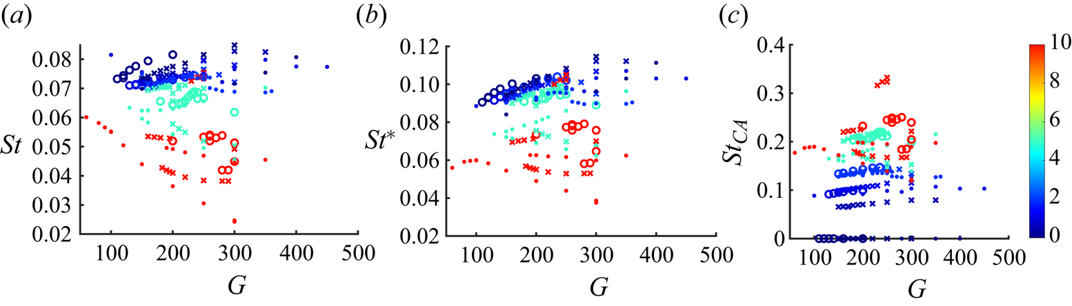
Our considerations are based on the close dependence of the variation of virtually all quantities on the instability amplitude, more accurately, on its square. This is a well-known theoretical result of the weakly nonlinear theory. In particular, the Landau model predicts a variation of angular frequency proportional to the square of the amplitude of the modelled oscillation. Zielinska et al. (Reference Zielinska, Goujon-Durand, Dušek and Wesfreid1997) evidenced and theoretically substantiated the same scaling for the mean value of the streamwise velocity of the cylinder wake. Though the theory originally concerns supercritical Hopf bifurcations close to their onset, we extend our ansatz to subcritical branches and strongly nonlinear regimes. It can be objected that the amplitude of oscillations is not an external parameter. However, mathematically, an unambiguous prediction based on external parameters is possible only for the asymptotic state, provided it is unique and thus independent of the initial conditions. This is not always the case due to the coexistence of solutions. More often, transient stages are to be accounted for: in numerical simulations, because of the simulation time; in experiments, because of material limitations. Conceptually, correlations between two (or more) variables resulting from observations are very frequent. For falling bodies, the correlation between the drag coefficient and the Reynolds can be cited as an example. As will be shown, the addition of this information solves the problem satisfactorily. The measure of the amplitude of oscillation is thus an important piece of information.
In spite of the detailed time series of all simulations at our disposal, we limit our analysis only to data we retrieved in the effort to establish the bifurcation diagrams of the preceding section. In the process, transient data was needed in some cases, e.g. to establish thresholds on the basis of growth rates or to investigate the stability of bi-stability branches. As a consequence, the processed ensemble contains relatively randomly chosen (chosen originally with a different purpose) transient and asymptotic data. To introduce some ‘noise’, we also kept data obtained with different computational accuracy when the reliability of the results had been checked. We believe that this mimics, to some extent, experimental conditions. The resulting ensemble includes 247 sets of data, each containing a single value for each of the most relevant quantities (values of external parameters, averages and amplitudes of velocity components of the cylinder centre, amplitude and period of vertical oscillations of the cylinder axis).
To allow easy comparison with other data available in the literature, we consider the drag coefficient and the Strouhal number as functions of the Reynolds and Galileo numbers (2.5) related by the relation
 \begin{equation} Re = Ga\langle u_z\rangle, \end{equation}
where  $\langle u_z\rangle$ is the average vertical velocity in our non-dimensionalisation.
5.1. Drag coefficient
The commonly used definition of the drag coefficient for oblong cylinders uses the constant projection  $Ld$ normal to the axis (Clift et al. Reference Clift, Grace and Weber1978) as the section perpendicular to the flow even if the cylinders fall freely and oscillate. For freely falling cylinders, the balance between the hydrodynamic force, the gravity and buoyancy relates the drag coefficient
 $C_d$ to the vertical velocity. In dimensional units (Toupoint et al. Reference Toupoint, Ern and Roig2019),
 \begin{equation} C_d= \frac{\rm \pi}{2} \frac{g_{eff} d}{\overline{u_z}^2},\end{equation}
where  $\overline {u_z}$ is the average (dimensional) vertical velocity. Given our non-dimensionalisation of the velocity by the velocity scale (2.1), the formula (5.2) becomes
 \begin{equation} C_d= \frac{2 d}{L} \frac{1}{\langle u_z\rangle^2}, \end{equation}
where  $\langle u_z\rangle$ is the average non-dimensionalised vertical velocity. In spite of the definition accounting for the cylinder length, it cannot be expected that the drag coefficient is independent of the aspect ratio, especially for moderate aspect ratios. This effect is already accounted for in table 6.1 of Clift et al. (Reference Clift, Grace and Weber1978). For this reason, we investigate each of the three aspect ratios
 $L/d=2,3,5$, separately.
Let us present the methodology for the length to diameter ratio of 5.
Results of 81 simulations are available in this case. Figure 18(a) shows that values of the drag coefficient in regimes with small or non-existent vertical oscillations are distributed along a single line, which represents a master curve for non-oscillating regimes. The larger the amplitude (represented by the colour bar), the larger the deviation from this curve. We shall set a lower limit for the amplitude of flutter at  $A(n_z)= A_{min}=0.15$. Out of the original 81 values, 54 lie below this limit. Lowering it from 0.15 to 0.05 reduces the number of ‘non-fluttering’ or ‘weakly fluttering’ regimes to 50, which does not significantly change the following analysis.
(a) Scatter plot of drag coefficient vs Reynolds number coloured as a function of the vertical oscillation amplitude  $A(n_z)$. The marker types indicate the density ratio:
 $\rho _s/\rho =0$, triangle;
 $\rho _s/\rho =1$, square;
 $\rho _s/\rho =2$, diamond;
 $\rho _s/\rho =5$, cross;
 $\rho _s/\rho =10$, circle. The colours of the colour bar quantify the oscillation amplitude. Full line: fit (5.4) of non oscillating or weakly oscillating data. (b) Drag correction with respect to the fit in (a) as a function of the square of oscillation amplitude (for colours, see the legend). Dotted lines: fit to the function 5.6. Here
 $L/d=5$.

The regimes with amplitudes less than  $A_{min}$ will be processed as ‘practically’ steady
 $A(n_z) \approx 0$. The aspect ratio having been fixed and steady states being independent of the density ratio, there remains a single variable function to be fitted to
 $Ga$ or, almost equivalently,
 $Re$. (Since
 $Re$ is related to
 $Ga$ by the vertical velocity, itself a dependent variable subject to variations, the fits are not exactly the same.)
Clift et al. (Reference Clift, Grace and Weber1978) provided correlations for cylinders of aspect ratios 1 through  $\infty$ (in table 6.1 of Clift et al. Reference Clift, Grace and Weber1978) as well as curves of drag coefficient vs Reynolds number in the steady regime at Reynolds numbers up to about 100. Their correlation results from a third degree polynomial fit of the logarithm of the Reynolds number vs the variable
 $w=\tfrac {1}{3}\log _{10}(C_d \,Re^2)$. The coefficients are given in table 6.1 of Clift et al. (Reference Clift, Grace and Weber1978) as functions of the aspect ratio
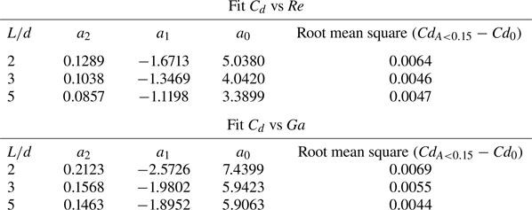
 $E=L/d$. In what follows, we use a simple second degree fit to the ensemble of drag coefficient values of weakly oscillating regimes:
 \begin{equation} \log(C_{d,0})= a_2 \log^2(Re) + a_1 \log(Re) + a_0. \end{equation}
Figure 19 presents the comparison of three fits: (i)  $C_{d,Clift}$ of Clift et al. (Reference Clift, Grace and Weber1978, table 6.1); (ii)
 $C_{d,fC}$ obtained by the method of Clift et al. (Reference Clift, Grace and Weber1978) applied to our data; (iii)
 $C_{d,0}$ given by (5.4). As can be seen, the difference between
 $C_{d,fC}$ and
 $C_{d,0}$ is of the order of
 $10^{-3}$ in the interval
 $50 \le Re \le 300$ and can be neglected. The original fit
 $C_{d,Clift}$ by Clift et al. (Reference Clift, Grace and Weber1978) agrees for
 $Re<50$ and overestimates the drag coefficient for higher Reynolds number values. The coefficients of the fit (5.4) are provided in table 11. The standard deviation from the fitted master curve is also presented and is less than 0.005.
Comparison of the correlation from table 6.1 of Clift et al. (Reference Clift, Grace and Weber1978) ( $C_{d,Clift}$) and of the fits of the computed drag coefficients for regimes where
 $A(n_z)<0.15$ using the method of Clift et al. (Reference Clift, Grace and Weber1978) (
 $C_{d,fC}$) and the second-degree formula (5.4) (
 $C_{d,0}$). The graphs of
 $C_{d,0}$ and
 $C_{d,fC}$ are practically superimposed. The enlarged difference
 $C_{d,0}-C_{d,fC}$ is seen in the inset.


The effect of the density ratio can be assessed from the marker types in figure 18(a). The largest upward deviation from  $C_{d,0}$ is observed for the density ratio 2 (diamonds), whereas the largest downward shift is obtained for the density ratio 10 (‘o’). At the density ratio 5, the drag coefficient remains close to the fitted curve. Qualitatively, it is clear that the deviation from the master curve depends on the oscillation amplitude and the density ratio.
It may, strictly speaking, vary also as a function of the Reynolds (Galileo) number. However, if the difference of the drag coefficient from the master curve  $dC_{d}= C_{d}-C_{d,0}$ is plotted vs the square of the amplitude (figure 18b), it is seen that
 $dC_{d}$ is quite well proportional to the square of amplitude of oscillations for a given density ratio independently of the Reynolds (Galileo) number. A simple polynomial fit as a function of the density ratio on the interval
 $[0,10]$ yields a satisfactory result but, since the drag coefficient remains finite at both ends of the interval
 $[0,\infty ]$ of density ratios, a transformation to a finite interval of the independent variable is more inadequate and provides the possibility of extrapolation to infinite density ratios. We shall use the transformation
 $[0,\infty ] \rightarrow [0,1]$:
 \begin{equation} s = \frac{r}{r_0 +r}, \end{equation}
where  $r$ denotes the density ratio
 $r \equiv \rho _s/\rho \in [0,\infty [$ and
 $s \in [0,1]$ is the new variable used for the regression. The parameter
 $r_0$ makes the distinction between ‘light’ and ‘dense’. We consider a global two-dimensional regression, with respect to both variables
 $s$ and
 $A^2(n_z)$ and linear in each of them:
 \begin{equation} C_d - C_{d,0} \approx dC_d = \left(c_1 s + c_2 \right) A^2(n_z)+ c_3. \end{equation}
The regression uses the whole sample (of 81 sets of simulation results for  $L/d=5$). The value of
 $r_0$ can be used for minimising the error and constitutes a fourth parameter of the fit. Increasing the degree of the regression brings no significant improvement and tends to yield spurious oscillations. Another method to improve the fit is to take account of the Reynolds number variation. This brings only a 10 % reduction of the (already small) error. The weak effect of the Reynolds number is in agreement with the general observation that the drag is almost independent of the Reynolds number starting from
 $Re=150$ (see Toupoint et al. Reference Toupoint, Ern and Roig2019, figure 7). As a result, the simple bi-linear fit (5.6) is satisfactory. Let us remark, that the amplitude of oscillations of the cylinder axis can be replaced by the amplitude of oscillations of the horizontal velocity because both are tightly correlated.
Figure 20 presents the slopes of the  $A^2(n_z)$ scalings as a function of the density ratio for all the three length-to-diameter ratios of cylinders. Note that, for
 $L/d=5$ the slopes become negative. For a comparison, a linear (one-dimensional) fit has been performed individually for each density ratio. The so-obtained slopes represent the exact trends uncorrelated with other density ratios. They are also represented in the figure. The coefficients
 $c_i$,
 $i=1,2,3$, of the least-squares fit as well as the optimal value of
 $r_0$ are provided in table 12. The small value of the coefficient
 $c_3$ correctly accounts of the fact that the lines in figure 18(b) should start at zero. Table 12 also contains the total error cumulating the errors of both fits (5.4) and (5.6). As can be seen, the difference between the computed and the fitted values is so small that it makes no sense to present a figure of the scatter of the fitted values to compare them with figure 18(a).
Fitted slopes  $(c_1 s + c_2 )$ of the
 $A^2(n_z)$ scalings (5.6). Dashed lines, fit vs
 $Re$; dash-dotted lines, fit vs
 $Ga$. The colours correspond to the aspect ratio (see legend). Extrapolations to infinite density ratio (values in brackets: fit vs
 $Ga$):
 $L/d=2: -0.09 (-0.16)$,
 $L/d=3: -0.18 (-0.20)$,
 $L/d=5: -0.44 (-0.53)$. The markers indicate the slopes obtained separately for each density ratio by a one-dimensional linear fit. Circles (triangles) refer to regression with the Reynolds (Galileo) number as the independent variable.


The correlations of the drag coefficient as a function of the Reynolds number are most common in the available literature. However, unlike the Galileo number, the Reynolds number is not an external parameter of the problem. The scatter of the vertical velocity in (5.1) influences the correlation (5.4) and thus also the drag correction (5.6). In tables 11 and 12 we also present the result of corresponding fits using the Galileo number as the independent variable:
 \begin{gather} \log(C_{d,0,Ga})= a_2 \log^2(Ga) + a_1 \log(Ga) + a_0, \end{gather}
 \begin{gather} C_d - C_{d,0,Ga} \approx dC_{d,Ga} = \left(c_1 s+ c_2\right) A^2(n_z)+ c_3. \end{gather}
Though the difference of the coefficients  $c_i$ in (5.6) and (5.8) seems to be non-negligible, the difference of resulting fits
 $C_{d,fit,Re}=C_{d,0}+dC_{d}$ and
 $C_{d,fit,Ga}=C_{d,0,Ga}+dC_{d,Ga}$ presents a smaller root mean square than the total error of the drag coefficient.
For  $L/d=3$ and 2, the processing follows exactly the same lines. A set of 114 simulation results has been processed for
 $L/d=3$. Figure 21(a) shows that the oscillations systematically increase the drag. As shown in figure 21(b) the drag correction still scales as the square of the amplitude. This is not necessarily expected for density ratios 5 and 10. For these density ratios the branches of large flutter are subcritical and disconnected from branches of small oscillations (see figure 14a) and the scaling cannot be substantiated by weakly nonlinear arguments. In spite of that, the
 $A^2(n_z)$ scaling still approximately holds. For example, at
 $\rho _s/\rho =5$, the five points corresponding to large values of amplitude and those of the supercritical branch of small oscillations are well aligned along the same straight line. Similarly as for
 $L/d=5$ the slopes decrease with increasing density ratio without, however, becoming negative. The overall fit (including that of the drag coefficient without oscillations (5.4) and that of the drag correction due to oscillation (5.6) yields an error as small as 0.0046 (see tables 11 and 12 for the values of coefficients and the errors).
(a) Scatter plot of drag coefficient vs Reynolds number coloured as a function of the vertical oscillation amplitude  $A(n_z)$. Full line: fit (5.4) of non-oscillating or weakly oscillating data. The marker types indicate the density ratio (see the caption of figure 18, except for density ratios 0.5 (squares) and 1.16 (asterisks)). (b) Drag correction with respect to the fit in figure (a) as a function of the square of oscillation amplitude. Dotted lines: fit to the function (5.6). Here
 $L/d=3$.

The case of  $L/d=2$ has been investigated in less detail. Although 52 simulations are available for the processing only 20 satisfy the criterion
 $A(n_z)>0.15$ (see figure 22). Qualitatively, there is much less difference between
 $L/d=2$ and 3 than between 3 and 5. The fit results are, again, presented in tables 11 and 12. For
 $\rho _s/\rho =0$, the drag correction values at large amplitude are not quite aligned. Obviously, the Galileo number dependence starts to play a role. This is due to the long array of simulations at
 $\rho _s/\rho =0$ in figure 12 spanning a long interval
 $Ga \in [115,200]$. In spite of that, the final error of the fit is smaller than 1 %.
(a) Scatter plot of drag coefficient vs Reynolds number coloured as a function of the vertical oscillation amplitude  $A(n_z)$. Full line: fit (5.4) of non-oscillating or weakly oscillating data. For the meaning of the marker types refer to caption of figure 18. (b) Drag correction with respect to the fit in (a) as function of the square of oscillation amplitude. Dotted lines: fit to the function 5.6. Here
 $L/d=2$.

All other quantities vary similarly with the growth of the square of amplitude. This is the case of, for example, the vertical velocity, the Reynolds number and the oscillation period. The latter is analysed using a similar method in the next subsection.
5.2. Strouhal number
In this section, we focus on the frequency of oscillations of the cylinder axis in the vertical direction. As a consequence, we discard the frequencies of the fluid modes where the direction of the axis remains horizontal (symmetric periodic and crosswise oscillating states). Though not all regimes, where vertical oscillations of the cylinder axis are observed, are pure flutter, the frequencies do not differ significantly except for the case of the weak quasi-periodic flutter for the aspect ratio 3 and density ratio 10 described in § 3.2.2. These frequencies are not considered either. This still leaves 231 out of the total of 247 sets of simulation results for the analysis.
In the available literature, there is no general consensus as for the non-dimensionalisation of the frequency of falling and fluttering oblong cylinders. Marchildon et al. (Reference Marchildon, Clamen and Gauvin1964) remarked that, unlike for the (fixed) infinite cylinder and its von Kármán vortex street, the cylinder diameter, as length scale in the definition of the Strouhal number, is to be replaced by  $\sqrt {Ld}$. For the velocity scale the (mean) vertical velocity of the fall is used. This yields
 \begin{equation} St = \frac{f \sqrt{Ld}}{\overline{u_z}} = \sqrt{\frac{L}{d}} \frac{1}{T \langle u_z\rangle}, \end{equation}
where the first expression is written in dimensional units and the second in the non-dimensionalisation of the present paper. Alternatively, Chow & Adams (Reference Chow and Adams2011) and Toupoint et al. (Reference Toupoint, Ern and Roig2019) use the gravitational velocity (1.2) as velocity scale. In the paper by Toupoint et al. (Reference Toupoint, Ern and Roig2019), this results in the non-dimensionalisation
 \begin{equation} St^* = \frac{f \sqrt{Ld}}{u_{g,eff}} = \sqrt{\frac{\rm \pi}{4}} \frac{L}{d} \frac{1}{T}, \end{equation}
where the second expression relates this Strouhal number to the inverse of period expressed in the non-dimensionalisation of the present paper. Chow & Adams (Reference Chow and Adams2011) provided an account, moreover, of the effect of density ratio and suggest that the Strouhal number
 \begin{equation} St_{CA} = \sqrt{\frac{\rho_s}{\rho}} St^*\end{equation}
should assume a constant value of  $1/7.91$ (0.126). Figure 23 compares the three different definitions of Strouhal numbers (5.9), (5.10) and (5.11) in light of our simulation data.


The Strouhal numbers  $St$ and
 $St^*$ yield similar plots because
 \begin{equation} St^*/St = \overline{u_z}/u_{g,eff},\end{equation}
i.e. the ratio  $St^*/St$ is equal to the mean vertical velocity non-dimensionalised by the gravitational velocity scale. This ratio is situated between 1.2 and 1.5 at Galileo numbers
 $150 \le Ga \le 300$ for all aspect and density ratios. The value assumed by Chow & Adams (Reference Chow and Adams2011) is 1.33 and data of Toupoint et al. (Reference Toupoint, Ern and Roig2019) also agree with these values. The factor
 $\sqrt {\rho _s/\rho }$ suggested by Chow & Adams (Reference Chow and Adams2011) over-compensates the effect of the density ratio (and makes no sense for very light bodies). Here
 $St^*$ concentrates the best the values for all the three aspect ratios for density ratios
 $\rho _s/\rho \le 2$. The average of 0.1 is in agreement with that of Toupoint et al. (Reference Toupoint, Ern and Roig2019). For larger density ratios (5 and 10), the values are considerably scattered both due to different aspect and density ratios. For this reason, we shall proceed similarly as in § 5.1 and treat each of the aspect ratios separately. Similarly as for the regression of the drag coefficient vs the Galileo number and the Reynolds number, it is practically indifferent whether the analysis is performed for
 $St$ or
 $St^*$ and whether the Reynolds or the Galileo number is taken as the independent variable. We shall choose
 $Ga$ as an independent variable and
 $St^*$ as a dependent variable.
Figure 24 presents scatter plots of  $St^*$ vs
 $Ga$ separately for each aspect ratio
 $L/d=2$,
 $3$ and 5. Markers identify the density ratios, the colouring indicates the amplitude of oscillations. The inertia plays a significant role for density ratios 5 (crosses) and 10 (circles) yielding significantly lower frequencies than for light bodies. The bi-stabilities emphasise the important role of the amplitude tending to lower the frequency (increase the period) in agreement with expectation namely if tumbling is approached for very large amplitude.
Scatter plots of the values of  $St^*$ (5.10) vs
 $Ga$ for the three aspect ratios: (a)
 $L/d=2$; (b)
 $L/d=3$; (c)
 $L/d=5$. The density ratios are identified by symbols of the legends, the amplitudes of oscillations are indicated by the colour bars. (d)
 $L/d=5$, fit: circles, exact values of
 $L/d=5$; crosses, fit (5.13) with coefficients given in table 13.

To obtain an accurate fit, it was seen in the case of the drag coefficient, that higher degree regression was needed. Moreover, the regression procedure could be split in two stages: a single-parameter fit of the master curve for negligible oscillations (independent of the density ratio) and a subsequent two-parameter regression accounting for oscillations. In contrast, the frequency depends on the density ratio whatever the oscillation amplitude making such a two step approach of little interest. To avoid too complicated and statistically unreliable correlations, we limit the regression to a tri-linear (linear in all of the three variables) fit as a function of  $G \equiv Ga$,
 $r \equiv \rho _s/\rho$ and
 $a^2 \equiv A^2(n_z)$. The main source of inaccuracy comes from the dependence on the density ratio which is not even monotonous, however we consider that more data are needed to account for this behaviour reliably. Testing of the error has shown that the transformation (5.5) yields monotonously decreasing error with increasing
 $r_0$, which means that a regression depending linearly directly on the density ratio
 $r$ performs the best. As a consequence, for each of the three aspect ratios, we determine the least-squares fit of
 \begin{equation} St^* \approx St^*_{fit} = c_1 r a^2 G +c_2 r G + c_3 r a^2 + c_4 r + c_5 a^2 G + c_6 G + c_7 a^2 + c_8 \end{equation}
and compute the relative root-mean-square error
 \begin{equation} \varepsilon = \frac{\sqrt{\sum_i (St^*_i - St^*_{fit,i})^2}}{\sqrt{\sum_i (St^*_i)^2}} \end{equation}
and maximum relative error
 \begin{equation} \varepsilon_{max} = \mbox{max} (|St^*_i - St^*_{fit,i}|/St^*_i). \end{equation}
The numerical values of the coefficients  $c_i$ of the fit (5.13) are given in table 13. The somewhat over-simplified tri-linear fit yields considerably larger errors than those obtained for the drag coefficient in table 12. Nevertheless, the several percent inaccuracy may be acceptable as a comprehensive summary of the obtained data. The worst case of aspect ratio
 $L/d=5$ is, moreover, represented graphically in figure 24 (scatter plot
 $L/d=5$, fit). The extreme values (corresponding to
 $\rho _s/\rho =0$ and 10) are well reproduced, the inaccuracies concern the intermediate density ratios.


6. Summary
In the present paper we have investigated the behaviour of freely falling cylinders of sufficient length-to-diameter ratio to assume a horizontal equilibrium position in the regime of steady free fall. Aspect ratios 2, 3 and 5 and solid-to-fluid-density ratios going from 0 to 10 in transitional regimes have been explored by numerical simulation. As third external parameter used to determine the thresholds of the transitional regimes we chose the Galileo number (2.5) related in a seemingly complicated way to the effective gravity and kinematic viscosity but appearing to be in agreement with the definition of the Archimedes number by other authors (Toupoint et al. Reference Toupoint, Ern and Roig2019). Both definitions account for the body volume, the only difference consisting in taking a unit cube instead of a unit sphere as a reference.
Several questions have been raised. The first issue aimed at exploring the onset of typical oscillations, called flutter (Toupoint et al. Reference Toupoint, Ern and Roig2019), yielding a planar trajectory of the cylinder centre with the cylinder axis oscillating vertically in the same plane. For each aspect ratio  $L/d=2$,
 $3$ and 5, a detailed analysis in the two-parameter
 $Ga$–
 $\rho _s/\rho$ plane has been performed. Since similar trajectories appear as the result of primary bifurcations of flat spheroids and flat cylinders keeping a vertical axis in laminar regimes, it could be expected that the fluttering regime would arise as the results of primary bifurcations the thresholds of which would be easy to determine. This expectation was confirmed for density ratios up to 2 and aspect ratios 2 and 3 but a much more complicated scenario was observed for larger density ratios and for cylinders of length 5
 $d$. For example, for
 $L/d=5$ and density ratio 0, no flutter at all was evidenced up to
 $Ga=400$. Instead, very small oscillations of high frequency were detected on the vertical velocity component while the trajectory of the cylinder centre remained strictly vertical. Given the small amplitude of these oscillations (less than 10
 $^{-4} \times$ smaller than the average vertical velocity itself), it was not initially evident that they were not of numerical origin. Given the several-orders-higher accuracy of the used numerical method, their presence starting at the same critical Galileo number at other density ratios and the independence of the result of the numerical accuracy this conjecture had to be discarded.
The negligible motion of the cylinder suggested the idea that the oscillations must be due to a purely fluid instability of the wake and must be evidenced in the wake of a fixed cylinder. This appeared to be the case and led to the identification of ‘fluid modes’ due to wake instabilities with negligible solid–fluid interaction. A particular feature of the primary instability of the wake of the fixed cylinder placed perpendicularly to the flow direction is that all symmetries remain preserved which enhances the difficulty of its detection. Similarly, as fluid modes evidenced for flat bodies (Dušek et al. Reference Dušek, Zhou and Chrust2021), they are characterised by a weak response of the solid body degrees of freedom to the unsteadiness of the wake. Unlike the robust fluttering motion, the fluid modes yield very early a chaotic motion with three-dimensional trajectories and horizontally rotating cylinder axis. For this reason, they can be associated with ‘irregular’ regimes evidenced experimentally by Toupoint et al. (Reference Toupoint, Ern and Roig2019). With increasing Galileo number, vertical oscillations progressively grow and the strongly oscillating fluid modes tend to the flutter, albeit imperfectly, having lost its perfect periodicity and symmetry.
The role of the length-to-diameter ratio is most conspicuous in the comparison of  $L/d=3$ and 5. It would certainly be interesting to undertake a finer increment (which would be feasible but would yield a large amount of additional data to process) of the aspect ratio and go beyond
 $L/d=5d$ (which causes technical difficulties in the numerical method used). Nevertheless, the practically opposite scenarios, where the flutter arises from a primary bifurcation for light cylinders of aspect ratio
 $L/d=3$ and for dense cylinders of aspect ratio
 $L/d=5$, indicate that for short oblong cylinders the inertia tends to inhibit the flutter whereas for longer ones the converse seems to be true. Such a contrast was not expected initially.
Another feature of the transition to the fluttering motion is the presence of subcritical effects, i.e. subcritical bifurcations yielding bi-stability. Similar effects were already observed for flat falling bodies such as oblate spheroids (Zhou et al. Reference Zhou, Chrust and Dušek2017). They are usually typical for larger density ratios. In the present work, they were evidenced for density ratios  $\rho _s/\rho \ge 2$. The subcritical branches (characterised by large oscillations) correspond to the flutter, the coexisting branches are rarely steady, instead, they correspond to unsteady fluid modes. The non-uniqueness of the asymptotic solutions implies a loss of predictability. The oscillation amplitude is then a necessary complement of information to provide the distinction between both alternatives.
Finally, we addressed the problem of scattered results reported in several experimental studies and making it difficult to propose a simple law predicting the drag of the freely falling cylinders and the frequency of their oscillations once path instabilities set in. Also our values of the drag coefficient as a function of the Reynolds number are significantly scattered off the master curve obtained by processing regimes without or with weak oscillations. To reproduce the scatter, it was necessary to account for the oscillation amplitude and for the density ratio that starts to be of importance once the unsteady effects become non-negligible. We suggested a simple bilinear fit of the deviation from the master curve of ‘steady drag’ yielding a prediction with an error of less than 1 % if the amplitude is provided and accounted for. It can be objected that the amplitude is an a posteriori piece of information. However, without it, bistable branches of solution cannot be distinguished and, conceptually, it is not different from the terminal Reynolds number, figuring in most experimental correlations, which is not an external parameter either. For the characterisation of the frequency, the Strouhal number introduced by Toupoint et al. (Reference Toupoint, Ern and Roig2019) was used as a dependent variable and the Galileo number was used as a parameter. A classical Strouhal number based on the vertical velocity and the length scale  $\sqrt {Ld}$ as suggested by Marchildon et al. (Reference Marchildon, Clamen and Gauvin1964) and the Reynolds number as the independent variable could also be considered. In this case, a three-dimensional tri-linear regression, accounting for the Galileo number, density ratio and the square of amplitude of vertical oscillations of the cylinder axis, yielded an acceptable approximation, albeit, with errors one order of magnitude larger than the fit of the drag coefficient. The origin of the error is due the actually more complex dependence on the density ratio, in the same way as for the drag correction. However, the amount of available data was not sufficient to use of a higher degree regression with enough reliability.
Our study attempted to bring more detailed information on the behaviour of freely falling oblong cylinders completing the experimental work of Toupoint et al. (Reference Toupoint, Ern and Roig2019). We believe that our numerical analysis has improved the understanding of this topic. The large number of simulations was enabled by the low cost of a single one. It was seen that the complexity of some states required very long runs but thanks to the efficiency of the spectral method each simulation can be run on a single thread. This means that, if a run takes a month, it is just 1 month of net CPU time with no need for costly massively parallel servers (where, nonetheless, large numbers of independent runs can be submitted simultaneously as an ideally parallel job). In future, the behaviour of longer cylinders is to be investigated. For this purpose, it will no longer be possible to use costly fully three-dimensional computation methods.
Acknowledgements
The authors are grateful to the ‘Centre de Calcul Intensif d'Aix-Marseille’ for granting us access to its high-performance computing resources.
Declaration of interests
The authors report no conflict of interest.