






1 Introduction and main result
Let
$f(z)=\displaystyle \sum _{\alpha \in \mathbb {N}^n}a_\alpha z^\alpha \in H(\mathbb {B}_n)$
 be an analytic function over the unit ball in
$\mathbb {C}^n$
 , and let
$X_0$
 be a random variable defined on a probability space
$(\Omega , \mathcal {F}, \mathbb {P})$
 . In this note, by a random analytic function (RAF), we mean the series

where
$\{X_\alpha \}_{\alpha \in \mathbb {N}^n}$
 is a sequence of independent and identically distributed (i.i.d.) random variables.
The convergence radius of
$\mathcal {R} f$
 is almost surely a constant, and to ensure that
$\mathcal {R} f$
 is an analytic function over
$\mathbb {B}_n$
 for any
$f \in H(\mathbb {B}_n)$
 , it is necessary and sufficient to have
$\limsup \limits _{|\alpha |\to \infty }|X_\alpha |^{\frac {1}{|\alpha |}}\leq 1$
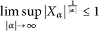 a.s. (see [Reference Shabat29, p. 32]. This requires
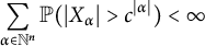
for some
$c\in (0,\infty )$
 . The condition is satisfied, in particular, if
$X_\alpha \in L^p(\Omega , \mathcal {F}, \mathbb {P})$
 for some
$p>0$
 .
The study of random series traces its roots back to the seminal work of Émile Borel in 1896 ([Reference Borel2] and [Reference Kahane16, p. 37]). Throughout its extensive history, the random operator
$\mathcal {R}f$
 has been the subject of rigorous scrutiny, with particular attention paid to the distribution of zero sets. Traditionally, the literature has centered on three canonical randomization methods (Gaussian, Rademacher, and Steinhaus) in Kahane’s monograph [Reference Kahane16]. A natural and recurring question concerns the behavior of randomization methods beyond these standard cases. While the impact of general distributions has been widely examined in the context of random polynomials (specifically regarding their zero sets), it remains relatively under explored in the realm of RAFs. A significant contribution is the study of the so-called “pits property” by Offord [Reference Offord25, Reference Offord26], which considered a general random variable
$X_0$
 , building upon the celebrated Littlewood–Offord results for the Rademacher case [Reference Littlewood and Offord23]. More recently, this line of inquiry has expanded to include stationary Gaussian processes [Reference Borichev, Nishry and Sodin3].
Attempts to move beyond the three canonical distributions generally rely on one of two strategies:
-
• Symmetry assumptions: Assuming $X_0$
 and
$-X_0$
share the same distribution allows for the application of Kahane’s reduction principle [Reference Kahane16, p. 9]. This powerful tool often reduces general problems to the Rademacher case. Additionally, symmetry grants access to the Lévy inequality [Reference Li and Queffélec18, Theorem III.2, p. 129].
-
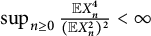
• Moment conditions: Imposing technical restrictions on moments, such as the condition $\sup _{n \ge 0} \frac {\mathbb {E}X_n^4}{(\mathbb {E}X_n^2)^2} < \infty $
found in [Reference Kahane16, Theorem 1, p. 54], or similar hypotheses detailed in [Reference Borichev, Nishry and Sodin3, Reference Offord25, Reference Offord26].


The objective of this note is to explore how the distribution of
$X_0$
 influences the properties of RAFs, while imposing as few constraints on
$X_0$
 as possible. We frame our study within the context of Littlewood’s theorem. Let
$f(z)=a_0 + a_1z + a_2z^2+\cdots \in H^{2}(\mathbb {D})$
 be an element of the Hardy space over the unit disk. Let
$\{\epsilon _n\}_{n\geq 0}$
 be a Rademacher sequence, that is, a sequence of i.i.d. random variables with
$\mathbb {P}(\epsilon _n = 1) = \mathbb {P}(\epsilon _n =-1)=\frac {1}{2}$
 for all
$n \geq 0$
 . Littlewood’s theorem, proved in 1930 [Reference Littlewood22], states that
$\mathcal {R} f(z) = \sum _{n=0}^{\infty }a_n\epsilon _nz^n\in H^p(\mathbb {D})$
 almost surely for all
$0<p<\infty $
 . When
$f \notin H^2(\mathbb {D})$
 , for almost every choice of signs,
$\mathcal {R} f$
 has a radial limit almost nowhere. The same is true for a standard Steinhaus sequence [Reference Littlewood21, Reference Paley and Zygmund27] and a standard Gaussian sequence [Reference Kahane16, p. 54], where standard Steinhaus (Gaussian) sequence is a sequence of i.i.d. standard Steinhaus (Gaussian) random variables. More generally, a Gaussian process version is obtained in [Reference Cheng, Fang, Guo and Liu6]. This work builds upon the recent findings of Chenget al. [Reference Cheng, Fang and Liu7], who established that for
$p,q,u\in (0,\infty )$
 and
$f(z)=\sum _{n=0}^{\infty } a_nz^n\in H(\mathbb {D})$
 , then

Here,
$\{X_n\}_{n\geq 0}$
 is a Rademacher (or standard Steinhaus (Gaussian)) sequence and

with
$M_p^q(r,f)=\left (\frac {1}{2\pi }\int _{0}^{2\pi }|f(re^{i\theta })|^{p}d\theta \right )^{\frac {q}{p}}$
 and
$ \|f\|_{p, q, u}=\left (\int _0^1(1-r)^{q u-1} M_p^q(r, f) d r\right )^{\frac {1}{q}}. $

A convenient way to reformulate this fact is to introduce the random symbol spaces. Let
$\mathcal {X}$
 be a Banach or
$p$
 -Banach space, with
$0<p<1$
 , of analytic functions over
$\mathbb {B}_n.$
 Define

If
$\{X_n\}_{n\geq 0}$
 is a Rademacher (or standard Steinhaus (Gaussian)) sequence, then we reformulate Littlewood’s theorem as

and (1) is

When
$\{X_n\}_{n\geq 0}$
 is a Rademacher (or standard Steinhaus (Gaussian)) sequence, the characterization of symbol spaces for other classical analytic function spaces can be found in [Reference Chen, Guo and Wang5, Reference Cheng, Fang, Liu and Lu8, Reference Fang and Tien11, Reference Fang and Tien12, Reference Karapetrović17]. In the context of Hardy spaces, the symbol space characterization for general i.i.d. random variables is established in [Reference Cai, Cheng, Fang and Liu4].
In the last paragraph of [Reference Cai, Cheng, Fang and Liu4], the authors raised a question concerning (2). The main purpose of this article is to give a complete solution to this problem for
$q\geq 4$
 .
Problem: Let
$p \in (0, \infty )$
 . How to characterize those
$X_0$
 ’s such that (2) holds?
There are two reasons why we choose to work with this problem:
(i) Given the absence of literature addressing the converse direction, it is natural to commence our investigation with one of the earliest and most fundamental results in the field.
(ii) The Littlewood theorem reformulated as (2) captures somehow the essence of randomization, at least in the framework of mixed norm spaces
$H^{p,q,u}(\mathbb {D})\ (0<p, q, u<\infty )$
 , in view of [Reference Cheng, Fang and Liu7, Theorem 6], which states that

under the three classical randomization methods.
One of our main results solves completely the above problem for
$q\ge 4$
 , hence extending Littlewood’s theorem in particular. We have the following theorem.
Theorem 1 Let
$\{X_n\}_{n\geq 0}$
 be a sequence of non-constant i.i.d. random variables and
$p,q,u\in (0,\infty )$
 . For
$4\leq q<\infty $
 ,
-
(i) if $0<p\leq 2$
, then
$(H^{p,q,u}(\mathbb {D}))_{\star }=H^{2,q,u}(\mathbb {D})$
if and only if
$X_0\in L^q(\Omega )$
; -
(ii) if $2<p<\infty $
, then
$(H^{p,q,u}(\mathbb {D}))_{\star }=H^{2,q,u}(\mathbb {D})$
if and only if
$X_0\in L^{q}(\Omega )$
and
$\mathbb {E} X_0=0$
.







Theorem 1 provides a complete characterization, in the critical range
$4\leq q<\infty $
 , of when the symbol-space identity
$\left (H^{p,q,u}(\mathbb {D})\right )_{\star }=H^{2,q,u}(\mathbb {D})$
 holds. We next turn to the subcritical regime
$0<q<4$
 . The following Theorem 2 shows that if the same identity is to remain valid, then the random variable
$X_0$
 must at least satisfy the corresponding
$L^q$
 -moment condition (and, when
$p>2$
 , the centering condition).
Theorem 2 Let
$\{X_n\}_{n\geq 0}$
 be a sequence of non-constant i.i.d. random variables and
$p,q,u\in (0,\infty )$
 . For
$0<q<4$
 ,
-
(i) if $0<p\leq 2$
,
$0<q<4,$
and
$(H^{p,q,u}(\mathbb {D}))_{\star }=H^{2,q,u}(\mathbb {D})$
, then
$X_0\in L^q(\Omega )$
; -
(ii) if $2<p<\infty $
,
$0<q<2,$
and
$(H^{p,q,u}(\mathbb {D}))_{\star }=H^{2,q,u}(\mathbb {D})$
, then
$X_0\in L^q(\Omega )$
; -
(iii) if $2<p<\infty $
,
$2\leq q<4,$
and
$(H^{p,q,u}(\mathbb {D}))_{\star }=H^{2,q,u}(\mathbb {D})$
, then
$X_0\in L^{q}(\Omega )$
and
$\mathbb {E} X_0=0$
.











Theorem 2 yields the necessary restrictions in the range
$0<q<4$
 , thereby delineating the admissible class of coefficient distributions for which the symbol-space identity can hold. The following Theorem 3 then proves that, under the natural
$L^4$
 -moment assumption (together with
$\mathbb {E} X_0=0$
 when
$p>2$
 ), these conditions indeed suffice, providing a matching sufficiency statement in this regime.
Theorem 3 Let
$\{X_n\}_{n\geq 0}$
 be a sequence of non-constant i.i.d. random variables and
$p,q,u\in (0,\infty )$
 . For
$0<q<4$
 ,
-
(i) if $0<p\leq 2$
and
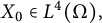
$X_0\in L^4(\Omega )$
, then
$(H^{p,q,u}(\mathbb {D}))_{\star }=H^{2,q,u}(\mathbb {D})$
; -
(ii) if $2<p<\infty $
,
$X_0\in L^{4}(\Omega ),$
and
$\mathbb {E} X_0=0$
, then
$(H^{p,q,u}(\mathbb {D}))_{\star }=H^{2,q,u}(\mathbb {D})$
.






The proofs of Theorems 1–3 are derived from Theorem 14, Proposition 16, and Theorem 18 in Section 3.
Theorem 4 Let
$\{X_n\}_{n\geq 0}$
 be a sequence of non-constant i.i.d. random variables and
$p,q,u\in (0,\infty )$
 . Let
$f(z)=\sum _{n=0}^{\infty } a_nz^n\in H(\mathbb {D})$
 and
$t=\max \{4,q\}.$

-
(i) For $0<p\leq 2$
and
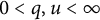
$0<q, u<\infty $
, if
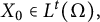
$X_0\in L^{t}(\Omega ),$
then $$ \begin{align*}\mathcal{R}f\in H^{p,q,u}(\mathbb{D})\ \text{a.s.}\Leftrightarrow\ \mathbb{E}\lVert\mathcal{R}f\rVert_{p,q,u}^{q}<\infty.\end{align*} $$
-
(ii) For $2<p<\infty $
and
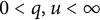
$0<q, u<\infty $
, if
$X_0\in L^{t}(\Omega )$
and
$\mathbb {E}X_0=0$
, then $$ \begin{align*}\mathcal{R}f\in H^{p,q,u}(\mathbb{D})\ \text{a.s.}\Leftrightarrow\ \mathbb{E}\lVert\mathcal{R}f\rVert_{p,q,u}^{q}<\infty.\end{align*} $$





Furthermore, we have investigated the symbol spaces of mixed norm spaces on the unit ball and obtained substantial results. Indeed, there exist several established results concerning the symbol spaces of analytic function spaces in higher dimensions: Hu and Shi [Reference Hu and Shi14] extended
$(\mathcal {M})_{\star }=\mathcal {D}$
 in [Reference Cochran, Shapiro and Ullrich9] to Dirichlet-type spaces over the unit ball under additional conditions. Moreover, Hu–Shi [Reference Shi and Hu30] gave sufficient conditions for
$(\mathcal {X})_{\star }$
 when
$\mathcal {X}$
 is
$H^{\infty }$
 or BMOA over the unit ball. Yu [Reference Yu34] proved that the boundary of the domain of convergence of a random multiple Taylor series is a natural boundary a.s. Li and Liu [Reference Li and Liu20] studied vector-valued random power series on the unit ball and obtained a vector-valued Salem–Zygmund theorem by using a martingale technique. For Bergman space in the unit ball, we can see [Reference Li, Wulan, Zhao and Zhu19, Reference Zhu37].
In this note, our first main focus is on mixed norm spaces of holomorphic functions on the unit ball
$\mathbb {B}_n\subset \mathbb {C}^{n}$
 ,
$\partial \mathbb {B}_n$
 its boundary. We let
$dv$
 denote the Lebesgue measure on
$\mathbb {C} ^{n}$
 , so normalized
$v(\mathbb {B}_n)=1$
 , and
$d\sigma $
 is the surface measure on
$\partial \mathbb {B}_n$
 normalized so that
$\sigma (\partial \mathbb {B}_n)$
 =1.
According to [Reference Shi and Ren31, Reference Zhang, Xiao and Hu35, Reference Zhou, Liang and Zeng36], a positive continuous function
$\varphi $
 on [0,1) is normal, if there exist
$0<a<b,0\leq r_0<1$
 such that
(i)
$\frac {\varphi (r)}{(1-r)^a}$
 is non-increasing for
$r_0\leq r<1$
 and
$\lim _{r\to 1^-}\frac {\varphi }{(1-r)^a}=0$
 ;
(ii)
$\frac {\varphi (r)}{(1-r)^b}$
 is non-decreasing for
$r_0\leq r<1$
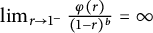
 and
$\lim _{r\to 1^-}\frac {\varphi (r)}{(1-r)^b}=\infty $
 .
For
$0<p<\infty ,0<q<\infty ,$
 and a normal function
$\varphi (r)$
 , let
$H^{p,q,\varphi }(\mathbb {B}_n)$
 denote the space of holomorphic
$f$
 on
$\mathbb {B}_n$
 , where

$M_p(r,f)=\left (\int _{\partial \mathbb {B}_n}|f(r\zeta )|^pd\sigma (\zeta )\right )^{\frac {1}{p}}$
 , and
$ \|f\|_{p, g, \varphi }=\left (\int _0^1(1-r)^{-1} \varphi ^q(r) M_p^q(r, f) d r\right )^{\frac {1}{q}}. $
 The Bergman spaces [Reference Zhu and Zhao38]

are special mixed norm spaces
$L_a^p(dv_\gamma )=H^{p,p,(1-r)^{\frac {\gamma +1}{p}}}(\mathbb {B}_n)$
 .
For high-dimension situation, we have the following results, which differ from their one-dimensional counterparts. However, as discussed in Remarks A and C, they are sharp under the present conditions.
Theorem 5 Let
$\{X_\alpha \}_{\alpha \in \mathbb {N}^n}$
 be a sequence of non-constant i.i.d. random variables and
$p,q\in (0,\infty )$
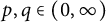 . Let
$\tau =\max \{2,q\}.$
 Assume that
$\varphi (r)$
 is a normal function and
$f(z)=\sum _{\alpha \in \mathbb {N}^n}a_\alpha z^\alpha \in H^{2,q,\varphi }(\mathbb {B}_n)$
 .
-
(i) For $0<p\leq 2$
and
$0<q<\infty ,$
if
$X_\alpha \in L^\tau (\Omega )$
, then
$\mathcal {R}f\in \ H^{p,q,\varphi }(\mathbb {B}_n)$
a.s. -
(ii) For $2<p<\infty $
and
$0<q<\infty ,$
if
$X_\alpha \in L^\tau (\Omega )$
,
$\mathbb {E} X_\alpha =0,$
and
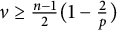
$\nu \geq \frac {n-1}{2}(1-\frac {2}{p})$
, then
$\mathcal {R}f\in \ H^{p,q,(1-r)^{\nu }\varphi }(\mathbb {B}_n)\ \text {a.s.}$






Theorem 5 provides the sufficiency direction for the randomization operator
$\mathcal {R}$
 : starting from
$H^{2,q,\varphi }(\mathbb {B}_n)$
 , one obtains mixed-norm control for
$\mathcal {R} f$
 (with the critical weight loss
$(1-r)^{\nu }$
 when
$p>2$
 ). The next theorem, Theorem 6, addresses the converse direction, showing that mixed-norm boundedness/integrability of
$\mathcal {R} f$
 forces the corresponding deterministic condition on
$f$
 .
Theorem 6 Let
$\{X_\alpha \}_{\alpha \in \mathbb {N}^n}$
 be a sequence of non-constant i.i.d. random variables and
$0<p,q<\infty $
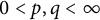 . Assume that
$\varphi (r)$
 is a normal function. If
$\mathcal {R}f\in H^{p,q,\varphi }(\mathbb {B}_n)$
 a.s. and
$X_\alpha \in L^4(\Omega )$
 , then
-
(i) $f\in H^{2,q,\varphi }(\mathbb {B}_n)$
when
$2\leq p<\infty $
; -
(ii) $f\in H^{2,q,(1-r)^{\nu }\varphi }(\mathbb {B}_n)$
when
$0<p<2$
and
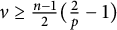
$\nu \geq \frac {n-1}{2}(\frac {2}{p}-1)$
.




Theorem 6 provides a converse implication, deriving deterministic mixed-norm conditions on
$f$
 from the almost sure finiteness of the mixed norm of the randomization
$\mathcal {R} f$
 . To enable moment-based arguments and obtain stronger integrability control, we next show Theorem 7.
Theorem 7 Let
$\{X_\alpha \}_{\alpha \in \mathbb {N}^n}$
 be a sequence of non-constant i.i.d. random variables and
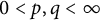
$0<p,q<\infty $
 . Let
$t=\max \{4,q\}$
 . Assume that
$\varphi (r)$
 is a normal function and
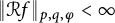
$\lVert \mathcal {R}f\rVert _{p,q,\varphi }<\infty $
 a.s.
-
(i) For $0<p<2$
and
$0<q<\infty ,$
if
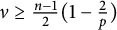
$\nu \geq \frac {n-1}{2}(\frac {2}{p}-1)$
and
$X_\alpha \in L^{t}(\Omega )$
, then $$ \begin{align*}\mathbb{E}\lVert\mathcal{R}f\rVert_{p,q,(1-r)^{\nu}\varphi}^q<\infty.\end{align*} $$
-
(ii) For $p=2$
and
$0<q<\infty ,$
if
$X_\alpha \in L^{t}(\Omega )$
, then $$ \begin{align*}\mathbb{E}\lVert\mathcal{R}f\rVert_{2,q,\varphi}^q<\infty.\end{align*} $$
-
(iii) For $2<p<\infty $
and
$0<q<\infty ,$
if
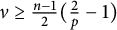
$\nu \geq \frac {n-1}{2}(1-\frac {2}{p})$
,
$\mathbb {E}X_\alpha =0,$
and
$X_\alpha \in L^{t}(\Omega )$
, then $$ \begin{align*}\mathbb{E}\lVert\mathcal{R}f\rVert_{p,q,(1-r)^{\nu}\varphi}^q<\infty.\end{align*} $$






We assume that all random variables are defined on a probability space
$(\Omega ,\mathcal {F},\mathbb {P})$
 with expectation denoted by
$\mathbb {E}(\cdot )$
 , where
$\mathcal {F}$
 is a
$\sigma $
 -algebra on
$\Omega $
 and
$\mathbb {P}$
 is a probability measure defined on
$\mathcal {F}$
 . The probability of an event
$\{\omega \in \Omega :\ X(\omega )\in A\}$
 , with
$A\in \mathcal {F}$
 , is
$\mathbb {P}(X\in A)$
 . The abbreviation “a.s.” stands for “almost surely.” As usual, “
$A\approx B$
 ” implies that there exists a positive constant
$C<\infty $
 such that
$\frac {A}{C}\leq B\leq CA$
 , “
$A\lesssim B$
 ” (resp. “
$A\gtrsim B$
 ”) means that there exists a positive constant
$C<\infty $
 such that
$A\leq CB$
 (resp.
$A\geq CB$
 ), and “
$\Leftrightarrow $
 ” stands for “if and only if.” Also, for the dyadic decomposition,
$I_k=\{n\in \mathbb {N}:\ 2^{k}\leq n<2^{k+1}\}$
 for integers
$k\geq 0$
 .
2 High-dimension situation
In this section, we study random symbol spaces for mixed norm spaces
$H^{p,q,\varphi }(\mathbb {B}_n)$
 of holomorphic functions on the unit ball
$\mathbb {B}_n\subset \mathbb {C}^n$
 , where
$\varphi $
 is a normal function. For i.i.d. random coefficients
$\{X_\alpha \}_{\alpha \in \mathbb {N}^n}$
 , we consider the randomization
$\mathcal {R} f(z)=\sum _{\alpha \in \mathbb {N}^n}a_\alpha X_\alpha z^\alpha $
 and the associated symbol class
$\left (H^{p,q,\varphi }(\mathbb {B}_n)\right )_{\star }$
 . Theorems 5 and 6 provide the basic sufficiency and necessity implications between membership of
$f$
 in
$H^{2,q,\varphi }(\mathbb {B}_n)$
 and almost sure membership of
$\mathcal {R} f$
 in
$H^{p,q,\varphi }(\mathbb {B}_n)$
 ; in higher dimension, a sharp, dimension-dependent loss
$(1-r)^\nu $
 appears when
$p\neq 2$
 . Theorem 7 then upgrades almost sure finiteness of the mixed norm to finiteness of its
$L^q(\Omega )$
 -moment under the stated hypotheses. A key technical ingredient is Lemma 8, which introduces the coefficient-multiplier operator
$f^{[\nu ]}$
 (defined by
$\frac {\Gamma (|\alpha |+\nu +1)}{\Gamma (|\alpha |+1)}$
 on Taylor coefficients) and the transform
$H_\nu f=(1-|z|^2)^{\nu }f^{[\nu ]}$
 , yielding the norm equivalence
$\|f\|_{p,q,(1-r)^\nu \varphi }$
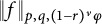 and isolating the dimensional loss.
Lemma 8 [Reference Shi and Ren31]
Let
$f\in H(\mathbb {B}_n)$
 ,
$0<p\leq \infty $
 ,
$0\leq \nu <\infty $
 , and
$\varphi $
 be normal. Then there exists a positive constant
$K$
 independent of
$f$
 , such that

where
$(H_{\nu }f)(z)=(1-|z|^2)^{\nu }f^{[\nu ]}(z)$
 and
$f^{[\nu ]}(z)=\displaystyle \sum _{\alpha \in \mathbb {N}^n}\frac {\Gamma (|\alpha |+\nu +1)}{\Gamma (|\alpha |+1)}a_{\alpha }z^{\alpha }$
 . Equivalently,

Let
$\mathcal {R} f(z)=\sum _{\alpha \in \mathbb {N}^n}a_\alpha X_\alpha z^\alpha $
 . For the convenience of the subsequent discussion, we denote
$\mathcal {R}_\epsilon f(z)=\sum _{\alpha \in \mathbb {N}^n}a_\alpha \epsilon _\alpha z^\alpha $
 , where
$\{\epsilon _\alpha \}_{\alpha \in \mathbb {N}^n}$
 is a sequence of i.i.d. Rademacher random variables.
Proof of Theorem 5
We first consider the symmetric case.
(i) Since
$\epsilon _{\alpha }(\omega ')X_{\alpha }(\omega )$
 and
$X_{\alpha }(\omega )$
 are identically distributed, provided that
$\{\epsilon _\alpha \}_{\alpha \in \mathbb {N}^n}$
 is a Rademacher sequence on a probability space
$\left (\Omega ',\mathcal {F}',\mathbb {P}'\right )$
 and independent to
$\{X_\alpha \}_{\alpha \in \mathbb {N}^n}$
 . Let

For
$q\leq p$
 , by Hölder’s inequality and Khintchine’s inequality, we have

For
$q>p$
 , by Minkowski’s inequality and Khintchine’s inequality, we have

So we have

where the “
$\lesssim $
 ” follows from (3) and (4), the “
$\leq $
 ” is obtained by applying Hölder’s inequality for
$0<q\leq 2$
 and Minkowski’s inequality for
$2<q<\infty $
 .
(ii) Similarly, we have

by Hölder’s inequality and Khintchine’s inequality when
$q\leq p$
 and by Minkowski’s inequality and Khintchine’s inequality when
$q>p$
 . Let

Let
$t_j:=|\zeta _j|^2$
 and
$\Delta _{n-1}:=\{t\in \mathbb {R}^n:\ t_j\geq 0$
 ,
$\sum _{j=1}^{n}t_j=1\}$
 . Then

and by
$Dirichlet$
 -
$\beta $
 integral [Reference Andrews, Askey and Roy1, p. 32],

We have

by Stirling’s formula. Since

and

we have

where
$\nu \geq \frac {n-1}{2}(1-\frac {2}{p})$
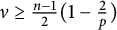 . By Lemma 8,

So,

where the first “
$\lesssim $
 ” holds by (6), the second one by Minkowski’s inequality and
$X_0\in L^{q}(\Omega )$
 for
$2<q<\infty $
 , and by Hölder’s inequality and
$X_0\in L^2(\Omega )$
 for
$0<q\leq 2$
 , and the last “
$\approx $
 ” due to (7).
For the non-symmetric case.
(i) We know that
$H^{2,q,\varphi }(\mathbb {B}_n)\subset \left (H^{2,q,\varphi }(\mathbb {B}_n)\right )_{\star }$
 by the proof of symmetric case. Since
$M_p^q(r,f)\leq M_2^q(r,f)$
 for
$0<p\leq 2$
 , we have
$\left (H^{2,q,\varphi }\left (\mathbb {B}_n\right )\right )_{\star }\subset \left (H^{p,q,\varphi }\left (\mathbb {B}_n\right )\right )_{\star }$
 . So,

(ii) Let
$\{\widetilde {X_\alpha }\}_{\alpha \in \mathbb {N}^n}$
 be an independent copy of
$\{X_\alpha \}_{\alpha \in \mathbb {N}^n}$
 . Then
$X_\alpha -\widetilde {X_\alpha }$
 is symmetric. Since
$\mathbb {E}X_\alpha =0$
 , we have

where
$(\mathcal {R} f)_{\omega }(z)=(\mathcal {R} f)(z)$
 ,
$(\widetilde {\mathcal {R} f})_{\omega '}(z)=\sum _{\alpha \in \mathbb {N}^n}a_{\alpha }\widetilde {X_\alpha }(\omega ')z^\alpha $
 , and

Since
$2<p<\infty $
 , by Minkowski’s inequality, we have

If
$1\leq q<\infty $
 , by Jensen’s inequality,

Then

By the proof of symmetric case, we have
$\mathbb {E}_\omega \mathbb {E}_{\omega '}\lVert (\mathcal {R}f)_{\omega }-(\widetilde {\mathcal {R}f})_{\omega '}\rVert _{p,q,(1-r)^{\nu }\varphi }^q<\infty $
 . So

Similarly, by Minkowski’s inequality, one has

If
$0<q<1$
 , then

By Hölder’s inequality and Fubini’s theorem,

By Hölder’s inequality and (6),

So, by Lemma 8,

Then
$\mathcal {R}f\in H^{p,q,(1-r)^{\nu }\varphi }(\mathbb {B}_n)$
 a.s.
For Bergman spaces
$L_a^p(dv_\gamma )$
 ,
$p\in (0,\infty )$
 , and
$\gamma \in (-1,\infty )$
 , we have the following corollary.
Corollary 9 Let
$\{X_\alpha \}_{\alpha \in \mathbb {N}^n}$
 be a sequence of i.i.d random variables and
$f\in L_a^2(dv_\gamma )$
 .
-
(i) For $0<p\leq 2$
, if
$X_\alpha \in L^2(\Omega )$
, then
$\mathcal {R}f\in \ H^{p,2,(1-r)^{\frac {\gamma +1}{2}}}(\mathbb {B}_n)$
a.s. -
(ii) For $2<p<\infty $
, if
$X_\alpha \in L^p(\Omega )$
,
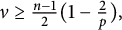
$\nu \geq \frac {n-1}{2}(1-\frac {2}{p}),$
and
$\mathbb {E}X_0=0$
, then $$ \begin{align*}\mathcal{R}f\in\ H^{p,2,(1-r)^{\frac{\gamma+1}{2}+\nu}}(\mathbb{B}_n)\ \text{a.s.}\end{align*} $$







Before proceeding to the proof of Theorem 6, we introduce a key result (Lemma 10) that plays a crucial role in the argument. To describe the boundary growth of functions in the mixed norm space, we consider the mixed norm

where
$M_2^2(r,f)=\sum _{m=0}^{\infty } r^{2m}\,\|f_m\|_{L^2(\partial \mathbb {B}_n)}^2$
 and
$f_m(z)=\sum _{|\alpha |=m}a_\alpha z^\alpha $
 . A key observation is that, as
$r\to 1^{-}$
 , the factor
$r^{2m}\approx e^{-2m(1-r)}$
 exhibits a pronounced scale-selection effect: at a boundary scale
$1-r\approx 2^{-k}$
 , the dominant contribution comes from degrees
$m\approx 2^{-k}$
 , while degrees much larger than this scale are exponentially suppressed. Motivated by this, we introduce a dyadic decomposition of the degrees
$I_k=[2^k,2^{k+1})$
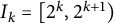 and measure the size of the
$k$
 -th “degree band” by
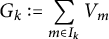
$G_k=\sum _{m\in I_k}\|f_m\|_{L^2(\partial \mathbb {B}_n)}$
 .
Lemma 10 Assume that
$f\in H^{2,q,\varphi }(\mathbb {B}_n)$
 ,
$q\in (0,\infty ),$
 and
$\varphi $
 is a normal function. Then

where
$G_k:=\displaystyle \sum _{m\in I_k}V_m$
 ,
$V_m:=\lVert f_m\rVert _{L^2(\partial \mathbb {B}_n)}^2$
 ,
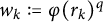
$w_k:=\varphi (r_k)^q$
 , and
$r_k=1-2^{-k}$
 .
The proof of Lemma 10 follows from [Reference Mateljevic and Pavlovic24, Theorem 2.1].
For
$p\in (0,1)$
 or
$q\in (0,1)$
 ,
$H^{p,q,\varphi }(\mathbb {B}_n)$
 is an
$s$
 -Banach space with
$s=\min \{p,q\}$
 [Reference Pavlović28, p. 83], that is,

We need the following lemma for the proof of Theorem 6, whose proof follows from the arguments similar to those of Theorem 8, Theorem 31 (Kahane’s inequality for
$p$
 -Banach space), and Theorem 28 (Fernique’s theorem for
$p$
 -Banach spaces) in [Reference Cheng, Fang and Liu7], hence skipped.
Lemma 11 Let
$0<p,q<\infty $
 ,
$\varphi $
 is a normal function, and
$\{X_\alpha \}_{\alpha \in \mathbb {N}^n}$
 be a standard random sequence. Let
$f(z)=\sum _{\alpha \in \mathbb {N}^n}a_\alpha z^\alpha \in H(\mathbb {B}_n)$
 . Then, the following statements are equivalent:
-
(i) $\mathcal {R} f\in H^{p,q,\varphi }(\mathbb {B}_n)$
a.s.; -
(ii) $\mathbb {E}(\lVert \mathcal {R} f\rVert _{H^{p,q,\varphi }}^t)<\infty $
for some
$t>0$
; -
(iii) $\mathbb {E}(\lVert \mathcal {R} f\rVert _{p,q,\varphi }^t)<\infty $
for any
$t>0$
; -
(iv) $\mathbb {E}\left (\exp \left (\lambda \lVert \mathcal {R} f\rVert _{H^{p,q,\varphi }}^s\right )\right )<\infty $
for small enough
$\lambda>0$
, where
$s=\min \{p,q,1\}$
.








Proof of Theorem 6
We first consider the symmetric case.
Since
$\epsilon _\alpha (\omega ')X_\alpha (\omega )$
 and
$X_\alpha (\omega )$
 have the same distribution, one has

where
$\{\epsilon _\alpha \}_{\alpha \in \mathbb {N}^n}$
 is a Rademacher sequence on a probability space
$\left (\Omega ',\mathcal {F}',\mathbb {P}'\right )$
 and independent to
$\{X_\alpha \}_{\alpha \in \mathbb {N}^n}$
 . Since
$\mathcal {R}f\in H^{p,q,\varphi }(\mathbb {B}_n)$
 a.s., it follows that for a.e.
$\omega '\in \Omega '$
 ,

Then, for a.e.
$\omega \in \Omega $
 ,
$\mathbb {P}_\epsilon \left (\mathcal {R}_\epsilon \mathcal {R}f\in H^{p,q,\varphi }(\mathbb {B}_n)\right )=1$
 . By Lemma 11,

(i) For
$2\leq p<\infty $
 and
$p\leq q$
 , by Hölder’s inequality and Khintchine’s inequality,

For
$2\leq p<\infty $
 and
$p>q$
 , by Minkowski’s inequality, Khintchine’s inequality, and Hölder’s inequality, one has

Then for a.e.
$\omega \in \Omega $
 ,

Since

and

by Lemma 10,

where
$r_k=1-2^{-k}$
 . We argue by contradiction. Suppose that

By (16), one has
$f\notin H^{2,q,\varphi }(\mathbb {B}_n)$
 . Combining this with (12) and (15), it suffices to show that

For
$\{(\alpha _1,\ldots ,\alpha _n)\}$
 , an order can be introduce by the following method. If

satisfy either of the following two conditions, then
$\alpha <\beta :$

(a)
$|\alpha |<|\beta |$
 ;
(b) if
$|\alpha |=|\beta |$
 , exists some
$k$
 ,
$1\leq k\leq n$
 , such that
$\alpha _1=\beta _1,\ldots ,\alpha _{k-1}=\beta _{k-1}$
 ,
$\alpha _k<\beta _k.$

The single-index sequences formed by arranging

in ascending order following the aforementioned order are denoted as
$\{b_l^{(k)}\}$
 ,
$\{c_l^{(k)}\},$
 and
$\{t_l^{(k)}\}$
 , respectively. Let

Write

and

Then

and

Since
$\mathbb {P}(|X_0|>0)>0$
 , write
$\mathbb {E}|X_0|^2:=\kappa>0$
 and
$\mathbb {E}|X_0|^4:=\lambda>0$
 . We have
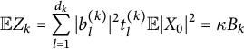
$\mathbb {E}Z_k=\displaystyle \sum _{l=1}^{d_k}|b_l^{(k)}|^2t_l^{(k)}\mathbb {E}|X_0|^2=\kappa B_k$
 and

So, by the Paley–Zygmund inequality [Reference Li and Queffélec18, Proposition III.3, p. 23], one has

Let
$\displaystyle (\frac {\kappa }{2})^{\frac {q}{2}}=c^{\prime }_1$
 . Then

If
$f\notin H^{2,q,\varphi }(\mathbb {B}_n)$
 , then
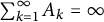
$\sum _{k=1}^{\infty }A_k=\infty $
 . Let

where
$J_1=\{1,\ldots ,t_1\}$
 and
$J_l=\{t_{l-1}+1,\ldots ,t_l\}$
 for
$l>1$
 , with the indices
$\{t_l\}_{l\geq 1}$
 chosen so that
$\displaystyle \sum _{k\in J_l}A_k\geq l$
 for all
$l$
 . We have

So,

and

By the Paley–Zygmund inequality again,

Since
$\sum _{l=1}^{\infty }\mathbb {P}\left (\{Y_l\geq \frac {1}{2}\mathbb {E}Y_l\}\right )=\infty $
 , by the Borel–Cantelli lemma,

And for a.e.
$\omega \in \Omega $
 ,

holds for infinitely many
$J_l$
 . Then

So
$\mathcal {R}f\notin H^{2,q,\varphi }(\mathbb {B}_n)$
 a.s., and one has
$\mathcal {R}f\notin H^{p,q,\varphi }(\mathbb {B}_n)$
 a.s.
(ii) For
$0<p<2$
 , similar to (13) and (14), by Hölder’s inequality, Khintchine’s inequality, and Minkowski’s inequality,

And

by Stirling’s formula. Then

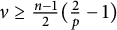
where
$\nu \geq \frac {n-1}{2}(\frac {2}{p}-1)$
 . So, by Lemma 8,

Then

That is, it suffices to prove that

when
$f\notin H^{2,q,(1-r)^{\nu }\varphi }(\mathbb {B}_n)$
 . The proof is similar to that of the case
$2\leq p<\infty $
 and is therefore omitted.
For the non-symmetric case.
(i) Since
$X_\alpha \in L^{4}(\Omega )$
 , by the symmetric case,

For
$2\leq p<\infty $
 , since
$M_2(r,\mathcal {R}f)^q\leq M_p(r,\mathcal {R}f)^q$
 , one has

(ii) For
$0<p<2$
 , if
$f\in (H^{p,q,\varphi }(\mathbb {B}_n))_{\star }$
 , then
$\mathcal {R}f\in H^{p,q,\varphi }(\mathbb {B}_n)$
 a.s. and
$\widetilde {\mathcal {R}f}\in H^{p,q,\varphi }(\mathbb {B}_n)$
 a.s.
If
$1\leq p<2$
 and
$0<q<1$
 , then

and

This implies that

and
$\mathcal {R}f-\widetilde {\mathcal {R}f}\in H^{p,q,\varphi }(\mathbb {B}_n)$
 a.s. So
$f\in H^{2,q,(1-r)^{\nu }\varphi }(\mathbb {B}_n)$
 by the symmetric case.
If
$1\leq p<2$
 and
$1\leq q<\infty $
 , then

and
$\mathcal {R}f-\widetilde {\mathcal {R}f}\in H^{p,q,\varphi }(\mathbb {B}_n)$
 a.s. Similarly,
$f\in H^{2,q,(1-r)^{\nu }\varphi }(\mathbb {B}_n)$
 .
If
$0<p,q<1$
 , then
$H^{p,q,\varphi }(\mathbb {B}_n)$
 is an
$s$
 -Banach space, where
$s=\min \{p,q\}$
 . So,

and
$\mathcal {R}f-\widetilde {\mathcal {R}f}\in H^{p,q,\varphi }(\mathbb {B}_n)$
 a.s. Hence,
$f\in H^{2,q,(1-r)^{\nu }\varphi }(\mathbb {B}_n)$
 .
If
$0<p<1$
 and
$1\leq q<\infty $
 , then

and

This implies that

and
$\mathcal {R}f-\widetilde {\mathcal {R}f}\in H^{p,q,\varphi }(\mathbb {B}_n)$
 a.s. Hence,
$f\in H^{2,q,(1-r)^{\nu }\varphi }(\mathbb {B}_n)$
 .
For Bergman spaces
$L_a^p(dv_\gamma )$
 ,
$p\in (0,\infty )$
 , and
$\gamma \in (-1,\infty )$
 , we have the following corollary.
Corollary 12 Let
$\{X_\alpha \}_{\alpha \in \mathbb {N}^n}$
 be a sequence of non-constant i.i.d random variables. Assume that
$p\in (0,\infty )$
 and
$\gamma \in (-1,\infty )$
 . If
$\mathcal {R}f\in L_a^p(dv_\gamma )\ \text {a.s.}$
 and
$X_\alpha \in L^4(\Omega )$
 , then
-
(i) for $2\leq p<\infty $
,
$f\in H^{2,p,(1-r)^{\frac {\gamma +1}{p}}}(\mathbb {B}_n)$
; -
(ii) for $0<p<2$
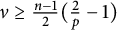
and
$\nu \geq \frac {n-1}{2}(\frac {2}{p}-1)$
,
$f\in H^{2,p,(1-r)^{\frac {\gamma +1}{p}+\nu }}(\mathbb {B}_n)$
.

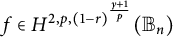


Corollary 12 specializes the converse principle to the Bergman spaces setting: assuming
$X_\alpha \in L^4(\Omega )$
 , almost sure membership
$\mathcal {R} f\in L_a^p(dv_\gamma )$
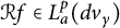 forces the corresponding deterministic mixed-norm regularity of
$f$
 (with the critical weight compensation when
$p<2$
 ). We then relax the i.i.d. hypothesis and allow merely independent coefficients satisfying uniform moment comparability and a variance lower bound; Proposition 13 shows that if
$f\notin H^{2,q,\varphi }(\mathbb {B}_n)$
 , then this failure propagates almost surely to the randomization, that is,
$\mathcal {R} f\notin H^{2,q,\varphi }(\mathbb {B}_n)$
 a.s.
Proposition 13 Let
$\{X_\alpha \}_{\alpha \in \mathbb {N}^n}$
 be a sequence of nonzero independent random variables,
$\varphi $
 be normal, and
$q\in (0,\infty )$
 . We assume
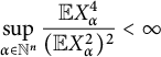
$\displaystyle \sup _{\alpha \in \mathbb {N}^n}\frac {\mathbb {E}X_\alpha ^4}{(\mathbb {E}X_\alpha ^2)^2}<\infty $
 and
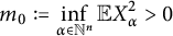
$m_0:=\displaystyle \inf _{\alpha \in \mathbb {N}^n}\mathbb {E}X_\alpha ^2>0$
 . If

then

Proof By Lemma 10, we only prove

when

Let
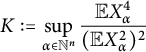
$K:=\displaystyle \sup _{\alpha \in \mathbb {N}^n}\frac {\mathbb {E}X_\alpha ^4}{(\mathbb {E}X_\alpha ^2)^2}$
 . Then
$\mathbb {E}|X_\alpha |^4\leq K\left (\mathbb {E}|X_\alpha |^2\right )^2$
 . The choice of
$\{b_l^{(k)}\}$
 ,
$\{c_l^{(k)}\}$
 ,
$\{t_l^{(k)}\}$
 ,
$B_k$
 ,
$Z_k$
 ,
$W_k$
 , and
$A_k$
 is the same as that in Theorem 6. Then

So, by the Paley–Zygmund inequality [Reference Li and Queffélec18, Proposition III.3, p. 23],


Write
$\tilde {c}_1:=(\frac {m_0}{2})^{\frac {q}{2}}$
 . We have
$\mathbb {P}(W_k\geq \tilde {c}_1A_k)\geq \tilde {c}_0$
 . Assume that

where
$J_l$
 is the same as
$J_l$
 defined in Theorem 6. Then
$\mathbb {E}Y_l\geq \tilde {c}_0\sum _{k\in J_l}A_k$
 and
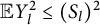
$\mathbb {E}Y_l^2\leq (S_l)^2$
 . So, by the Paley–Zygmund inequality [Reference Li and Queffélec18, Proposition III.3, p. 23],

and

Then
$\mathbb {P}(\{Y_l\geq \frac {1}{2}\mathbb {E}Y_l\}\ i.o.)=1$
 by the Borel–Cantelli lemma. So, we have that for a.e.
$\omega \in \Omega $
 ,

holds for infinitely many
$J_l$
 . Then
$\sum _{k=1}^{\infty }W_k=\sum _{l=1}^{\infty }\sum _{k\in J_l}W_k=\infty $
 a.s. That is,

For
$n=1$
 , by Proposition 13, we have: Let
$\{X_n\}_{n\geq 0}$
 be a sequence of nonzero independent random variables and
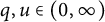
$q,u\in (0,\infty )$
 . Assume that

If
$f(z)=\sum _{n=0}^{\infty }a_nz^n\notin H^{2,q,u}(\mathbb {D})$
 , then

We now proceed to prove Theorem 7.
Proof of Theorem 7
(i) For
$0<p<2$
 , assume that

Since
$M_p^q(r,\mathcal {R}f)\leq M_2^q(r,\mathcal {R}f),$
 one has

By Jensen’s inequality for
$0<q\leq 2$
 and Minkowski’s inequality for
$2<q<\infty ,$


By (19)–(21),
$\lVert f\rVert _{2,q,(1-r)^\nu \varphi }=\infty $
 . Therefore, by Theorem 6 and the Kolmogorov zero-one law, for
$0<p<2$
 ,

which contradicts the assumption
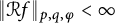
$\|\mathcal {R}f\|_{p,q,\varphi }<\infty $
 a.s.
(ii) For
$p=2$
 , the proof is similar to the case
$0<p<2$
 .
(iii) For
$2<p<\infty $
 and
$1\leq q<\infty ,$
 assume that
$\mathbb {E}\lVert \mathcal {R}f\rVert _{p,q,(1-r)^\nu \varphi }^q=\infty $
 . By (8) of Theorem 5,

Then

So, by (8) of Theorem 5,
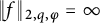
$\lVert f\rVert _{2,q,\varphi }=\infty $
 . It follows from Theorem 6 that
$\mathcal {R}f\notin H^{p,q,\varphi }(\mathbb {B}_n)$
 a.s., which contradicts the assumption
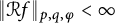
$\|\mathcal {R}f\|_{p,q,\varphi }<\infty $
 a.s.
For
$2<p<\infty $
 and
$0<q<1$
 , by (10) and (11) of Theorem 5, one has

The rest of the proof is analogous to that for the case
$2<p<\infty $
 and
$1\leq q<\infty $
 .
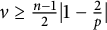
Remark A The restrictions in Theorems 5 and 6 are essentially sharp within our approach. First, the critical loss
$(1-r)^{\nu }$
 with
$\nu \geq \frac {n-1}{2}|1-\frac {2}{p}|$
 matches the worst-case degree growth in the spherical
$L^p-L^2$
 comparison (via the Stirling estimate for the monomial integral
$I(p)$
 ), hence it cannot be lowered in general. Second, the moment assumptions on
$X_0$
 (only
$L^2$
 for
$q\leq 2$
 , but
$L^q$
 for
$q>2$
 , and
$\mathbb {E} X_0=0$
 when
$p>2$
 ) are exactly those needed to close the Khintchine and Minkowski inequalities in the proof, so they are likewise not relaxable in this framework.
3 One-dimensional situation
As a special case, when
$n=1$
 and
$\varphi (r)=(1-r)^{u}$
 is comparable to a power weight, we recover and significantly sharpen these results for mixed norm spaces on unit disk
$\mathbb {D}$
 .
Theorem 14 Let
$\{X_n\}_{n\geq 0}$
 be a sequence of non-constant i.i.d. random variables and
$p,q,u\in (0,\infty )$
 . Let
$\tau =\max \{2,q\}.$

-
(i) For $0<p\leq 2$
and
$0<q,u<\infty ,$
if
$X_0\in L^{\tau }(\Omega ),$
then $$ \begin{align*}H^{2,q,u}(\mathbb{D})\subset\left(H^{p,q,u}\left(\mathbb{D}\right)\right)_{\star}.\end{align*} $$
-
(ii) For $2<p<\infty $
and
$0<q,u<\infty ,$
if
$X_0\in L^{\tau }(\Omega )$
and
$\mathbb {E}X_0=0$
, then $$ \begin{align*}H^{2,q,u}(\mathbb{D})\subset\left(H^{p,q,u}(\mathbb{D})\right)_{\star}.\end{align*} $$


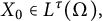





Proof We first consider the symmetric case. Since
$\mathbb {E} X_0=0$
 , the proof of (ii) is analogous to that of (i). Therefore, it suffices to prove (i).
(i) Since
$\mathcal {R} f(z)=\sum _{n=0}^{\infty }a_n X_n z^n$
 and
$\mathcal {R}_\epsilon \mathcal {R} f(z)=\sum _{n=0}^{\infty }a_n \epsilon _n X_n z^n$
 are identically distributed, where
$\{\epsilon _n\}_{n\geq 0}$
 is a Rademacher sequence on a probability space
$(\Omega ',\mathcal {F}',\mathbb {P}')$
 and independent to
$\{X_n\}_{n\geq 0}$
 . Then

Furthermore, one has

Now, we will prove (23). For
$p\geq q,$
 on the one hand, by Hölder’s inequality and Khintchine’s inequality,

On the other hand, by Jensen’s inequality and Khintchine’s inequality,

So, (23) is established for
$p\geq q.$
 For
$p<q$
 , the proof is similar to that of
$p\geq q.$

Hence, for
$0<q\leq 2$
 , by (23) and Hölder’s inequality,

For
$2<q<\infty $
 , by Minkowski’s inequality, one has

Then
$\mathbb {E}\lVert \mathcal {R}f\rVert _{p,q,u}^q\leq \mathbb {E}|X_0|^\tau \lVert f\rVert _{2,q,u}^q<\infty .$

For the non-symmetric case. From (22), (23), and the result of the symmetric case, the proof for the non-symmetric case is similar to that of the non-symmetric case in Theorem 5 and is therefore omitted.
Remark B The result
$X_0\in L^q(\Omega )$
 for
$2<q<\infty $
 of the above theorem is sharp under our conditions, since by [Reference Jevtić, Vukotić and Arsenović15, Lemma 4.2.7], we have

if and only if

That is, we need to estimate
$\mathbb {E}_X\left (\sum _{k\in I_n}|a_k|^2|X_k|^2\right )^{\frac {q}{2}}$
 when
$2<q<\infty $
 . So, by Minkowski’s inequality,

If
$X_0\notin L^q(\Omega )$
 , Proposition 16 implies that
$H^{2,q,u}(\mathbb {D})\subset (H^{p,q,u}(\mathbb {D}))_{\star }$
 fails.
Before establishing the necessary conditions on
$X_0$
 for
$H^{2,q,u}(\mathbb {D})\subset \left (H^{p,q,u}(\mathbb {D})\right )_{\star }$
 , we present the following lemma.
Lemma 15 [Reference Jevtić, Vukotić and Arsenović15, Theorem 8.1.1]
Let
$f(z)=\sum _{n=0}^{\infty }a_nz^{k(n)}$
 , where
$k(0)=0$
 and
$k(n)\in [2^{n-1},2^n)$
 ,
$n\geq 1$
 . Then
$f\in H^{p,q,u}(\mathbb {D})$
 if and only if
$\{2^{-nu}a_n\}\in l^q$
 .
Proposition 16 Let
$\{X_n\}_{n\geq 0}$
 be a sequence of non-constant i.i.d. random variables and
$p,q,u\in (0,\infty )$
 .
-
(i) For $0<p\leq 2$
,
$0<q<\infty $
, if
$H^{2,q,u}(\mathbb {D})\subset \left (H^{p,q,u}(\mathbb {D})\right )_{\star }$
, then
$X_{0}\in L^{q}(\Omega )$
. -
(ii) For $2<p<\infty $
,
$0<q<2$
, if
$H^{2,q,u}(\mathbb {D})\subset \left (H^{p,q,u}(\mathbb {D})\right )_{\star }$
, then
$X_{0}\in L^{q}(\Omega )$
. -
(iii) For $2<p<\infty $
,
$2\leq q<\infty $
, if
$H^{2,q,u}(\mathbb {D})\subset \left (H^{p,q,u}(\mathbb {D})\right )_{\star }$
, then
$X_0\in L^{q}(\Omega )$
and
$\mathbb {E} X_0=0$
.











Proof The proof of (ii) is identical to that of (i), so we only prove (i).
(i) Assume that
$f(z)=\sum _{n=0}^{\infty }a_n z^{k(n)}\in H^{2,q,u}(\mathbb {D})$
 . Since

by Lemma 15,

Write
$c_n:=a_n 2^{-nu}$
 . Then
$\{c_n\}_{n\geq 0}\in l^q$
 and (24) can be rewritten as

Assume
$X_0\notin L^{q}(\Omega )$
 . Let
$K_0:=|X_0|^q$
 and
$K_n:=|X_n|^q$
 . Then

Next, we will construct a sequence
$\{k_n\}_{n\geq 0}\in l^q$
 that violates (25), thereby contradicting (24). Let
$\{s_m\}_{m\geq 0}$
 be a sequence such that
$s_m\geq m^4$
 and

Then

Partition
$\mathbb {N}$
 into a sequence of consecutive finite blocks
$\{H_m\}_{m=1}^\infty $
 , which satisfies
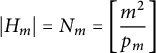
$|H_m|=N_m=\displaystyle \left [\frac {m^2}{p_m}\right ]$
 . We denote
$k_n:=\displaystyle \left (\frac {1}{s_m}\right )^{\frac {1}{q}},$
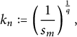 where
$n\in H_m$
 . Since
$s_mp_m\geq m^4$
 , we have

So,
$\{k_n\}_{n\geq 1}\in l^q$
 . Let
$E_m:=\{\omega :\ \exists \ n\in H_m,\ K_n(\omega )>s_m\}$
 . Then

So,
$\sum _{m=1}^{\infty }\mathbb {P}(E_m^{c})<\infty $
 . By the Borel–Cantelli lemma,
$\mathbb {P}(E_m^{c}\ i.o.)=0$
 . That is,
$\mathbb {P}(\liminf _{m\to \infty }E_m)=1$
 . Then

where
$m$
 is large enough. So,

Contradiction.
(iii) The proof for
$X_0\in L^q(\Omega )$
 is similar to that of (i). It is sufficient to prove that
$\mathbb {E} X_0=0$
 . If
$\mathbb {E} X_0\neq 0$
 , we take
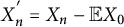
$X_n^{'}=X_n-\mathbb {E} X_0$
 , then
$\mathbb {E} X_n^{'}=0$
 . Since

we pick any
$\sum _{n=0}^{\infty }c_n z^n\in H^{2,q,u}(\mathbb {D})\backslash H^{p,q,u}(\mathbb {D})$
 with
$p>2$
 . By Theorem 14, one has

which contradicts (26).
Next, we provide sufficient conditions on
$X_0$
 for
$\left (H^{p,q,u}(\mathbb {D})\right )_{\star }\subset H^{2,q,u}(\mathbb {D})$
 . To this end, we need the following lemma.
Lemma 17 [Reference Sledd32, Lemma 14]
Let
$0<q\leq \infty $
 and
$u>0$
 . Then,

if and only if
$\{n^{-u}a_n\}\in l(2,q)$
 .
The sequential version of the mixed norm space
$l(p,q)$
 with
$0<p,q\leq \infty $
 [Reference Jevtić, Vukotić and Arsenović15] consists of complex sequences
$\{a_n\}_{n\geq 0}$
 such that

where we recall that
$I_k=\{n\in \mathbb {N}: 2^{k}\leq n<2^{k+1}\}$
 when
$k\geq 0$
 .
Theorem 18 Let
$\{X_n\}_{n\geq 0}$
 be a sequence of non-constant i.i.d. random variables and
$p,q,u\in (0,\infty )$
 . If
$X_0\in L^4({\Omega })$
 and
$\mathcal {R}f(z)=\sum _{n=0}^{\infty }a_nX_nz^n\in H^{p,q,u}(\mathbb {D})\ \text {a.s.},$
 then

Proof We first consider the symmetric case.
Since
$\epsilon _n(\omega ')X_n(\omega )$
 is identical distribution with
$X_n(\omega )$
 , we have

where
$\{\epsilon _n\}_{n\geq 0}$
 is a Rademacher sequence on a probability space
$(\Omega ',\mathcal {F}',\mathbb {P}')$
 and independent to
$\{X_n\}_{n\geq 0}$
 . Since
$\mathcal {R}f\in H^{p,q,u}(\mathbb {D})$
 a.s. and for a.e.
$\omega '\in \Omega '$
 ,

by [Reference Li and Queffélec18, Proposition III.7], we have that for a.e.
$\omega \in \Omega $


By [Reference Cheng, Fang and Liu7, Theorem 8],

Moreover, since

it follows that
$\mathcal {R}f\in H^{2,q,u}(\mathbb {D})$
 a.s. That is,

Suppose that
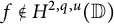
$f\notin H^{2,q,u}(\mathbb {D})$
 . It suffices to prove that
$\mathcal {R}f\notin H^{2,q,u}(\mathbb {D})$
 a.s. By Lemma 17, that is, if

it suffices to show that

The remainder of the proof of is similar to that of the symmetric case in Theorem 6 and is therefore omitted.
For the non-symmetric case. Making use of the result from the symmetric case, the proof for the non-symmetric case is similar to that of the non-symmetric case in Theorem 6 and is therefore omitted.
Theorem 18 yields a stronger result than Theorem 6 in the higher-dimensional setting. We now proceed to the proof of Theorem 4.
Proof of Theorem 4
It is sufficient to prove that

(i) Suppose that
$\{X_n\}_{n\geq 0}$
 is symmetric and
$\mathbb {E}\lVert \mathcal {R}f\rVert _{p,q,u}^q=\infty $
 . Combining (22) and (23), one has

Then
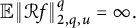
$\mathbb {E}\lVert \mathcal {R}f\rVert _{2,q,u}^q=\infty .$
 If
$0<q\leq 2$
 , then

So,
$\lVert f\rVert _{2,q,u}=\infty $
 . By Theorem 18,
$\mathbb {P}(\lVert \mathcal {R}f\rVert _{p,q,u}=\infty )>0$
 , a contradiction.
If
$2<q<\infty $
 , similarly, assume
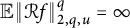
$\mathbb {E}\lVert \mathcal {R}f\rVert _{2,q,u}^q=\infty $
 . Since

we have
$\lVert f\rVert _{2,q,u}^q=\infty $
 . By Theorem 18,
$\mathbb {P}(\lVert \mathcal {R}f\rVert _{p,q,u}=\infty )>0$
 , a contradiction.
Assume that
$\{X_n\}_{n\geq 0}$
 is non-symmetric. For
$0<p\leq 2$
 , if
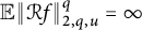
$\mathbb {E}\lVert \mathcal {R}f\rVert _{2,q,u}^q=\infty $
 , then
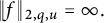
$\lVert f\rVert _{2,q,u}=\infty $
 . Since
$M_p^q(r,\mathcal {R}f)\leq M_2^q(r,\mathcal {R}f)$
 , one has
$\mathbb {E}\lVert \mathcal {R}f\rVert _{p,q,u}^q\leq \mathbb {E}\lVert \mathcal {R}f\rVert _{2,q,u}^q$
 . If
$\mathbb {E}\lVert \mathcal {R} f\rVert _{p,q,u}^q=\infty ,$
 then
$\lVert f\rVert _{2,q,u}=\infty .$
 So, by Theorem 18,
$\mathbb {P}(\lVert \mathcal {R}f\rVert _{p,q,u}=\infty )>0$
 , a contradiction.
(ii) For
$2<p<\infty $
 and
$1\leq q<\infty $
 , suppose that
$\mathbb {E}\lVert \mathcal {R}f\rVert _{p,q,u}^q=\infty $
 . By (9),
$\mathbb {E}\lVert \mathcal {R}f\rVert _{p,q,u}^q\leq \mathbb {E}\lVert \mathcal {R}f-\widetilde {\mathcal {R}f}\rVert _{p,q,u}^q.$
 From the proof of (i), we have
$\lVert f\rVert _{2,q,u}=\infty $
 . So, by Theorem 18,
$\mathbb {P}(\lVert \mathcal {R}f\rVert _{p,q,u}=\infty )>0$
 . This leads to a contradiction. For
$2 < p <\infty $
 and
$0 < q < 1$
 , the proof is similar to the case
$2 < p < \infty $
 and
$1 \leq q < \infty ,$
 and is therefore omitted.
Remark C The one-dimensional case is substantially stronger because the boundary geometry degenerates: on
$\partial \mathbb {D,}$
 we have
$|e^{ik\theta }|=1$
 , hence the
$L^p$
 -norms of monomials are independent of the degree
$k$
 , and the degree-dependent
$L^p-L^2$
 growth responsible for the higher-dimensional loss disappears when
$n=1$
 . Consequently, one can obtain lossless results under the original weight (see Theorem 14), unlike the ball case where an extra factor
$(1-r)^\nu $
 is unavoidable.
4 Example
Two classes of examples of general interests are presented in this section. These examples served as test cases in our research and may prove useful in other contexts.
4.1 Decreasing Taylor coefficients
Proposition 19 Let
$\{X_n\}_{n\geq 0}$
 be a sequence of non-constant i.i.d. random variables and
$p,q,u\in (0,\infty )$
 . Let
$f(z)=\sum _{n=0}^{\infty }a_n z^n\in H(\mathbb {D})$
 and
$\{|a_n|\}_{n\geq 0}$
 be a decreasing sequence. If
$\mathcal {R}f\in H^{p,q,u}(\mathbb {D})$
 a.s., then

The proof is based on the following lemma.
Lemma 20 (Chernoff’s inequality) [Reference Vershynin33, p. 18]
Let
$\{X_i\}_{i=1}^{N}$
 be independent Bernoulli random variables with parameters
$\{p_i\}_{i=1}^{N}$
 . Consider their sum
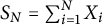
$S_N=\sum _{i=1}^{N}X_i$
 and denote its mean by
$u=\mathbb {E}S_N$
 . Then for any
$t<u$
 , we have

Proof of Proposition 19
We first consider the symmetric case.
Suppose that
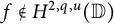
$f\notin H^{2,q,u}(\mathbb {D})$
 . By the proof of Theorem 18, it suffices to prove that

By Lemma 17, we show that

Let
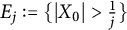
$E_j:=\{|X_0|>\frac {1}{j}\}$
 . Then
$\{|X_0|>0\}=\bigcup _{j=1}^{\infty } E_j$
 . Since
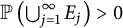
$\mathbb {P}\left (\bigcup _{j=1}^{\infty } E_j\right )>0$
 , there exists some
$j>0$
 such that
$\mathbb {P}(E_j)=:h>0$
 . We have that for every
$\omega \in \Omega $
 ,

where
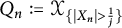
$Q_n:=\mathcal {X}_{\{|X_n|>\frac {1}{j}\}}$
 . Let
$C_k=\sum _{n\in I_k}Q_n$
 . Then
$\mathbb {E}C_k=h2^k$
 . Let

One has

by Lemma 20. So,
$\sum _{k=1}^{\infty }\mathbb {P}(\Omega _k)<\infty $
 . This implies that

by the Borel–Cantelli lemma. That is,

Let
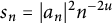
$s_n=|a_n|^2n^{-2u}$
 . Since
$\{|a_n|\}$
 is decreasing, for a.e.
$\omega \in \Omega $
 , one has
$s_n\geq s_{n+1}$
 and

when
$k$
 is large enough. Since
$2^{k+1}s_{2^{k+1}-1}\geq \sum _{n\in I_{k+1}}s_n$
 , we have

when
$N$
 is large enough. So,
$\sum _{k=1}^{\infty }\left (\sum _{n\in I_k}s_nQ_n\right )^{\frac {q}{2}}=\infty $
 a.s. By (27), that is,

For the non-symmetric case. The proof for the non-symmetric case is analogous to the that of the non-symmetric in Theorem 6.
Combining this with Theorem 14, we obtain the following conclusion.
Corollary 21 Let
$\{X_n\}_{n\geq 0}$
 be a sequence of non-constant i.i.d. random variables and
$p,q,u\in (0,\infty )$
 . Let
$\tau =\max \{2,q\}.$
 Assume that
$f(z)=\sum _{n=0}^{\infty }a_n z^n\in H(\mathbb {D})$
 and
$\{|a_n|\}_{n\geq 0}$
 is a decreasing sequence. Then,

if
$p,q,X_0$
 satisfy one of the following conditions:
-
(i) $0<p\leq 2$
,
$0<q, u<\infty ,$
and
$X_0\in L^{\tau }(\Omega )$
; -
(ii) $2<p<\infty $
,
$0<q, u<\infty $
,
$X_0\in L^{\tau }(\Omega ),$
and
$\mathbb {E}X_0=0$
.





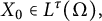

For Bergman space, by [Reference Hedenmalm, Korenblum and Zhu13, p. 2], we have the following corollary.
Corollary 22 Let
$\{X_n\}_{n\geq 0}$
 be a sequence of non-constant i.i.d. random variables and
$dA_\gamma (z)=(\gamma +1)(1-|z|^2)^\gamma dA(z)$
 . Assume that
$f(z)=\sum _{n=0}^{\infty }a_nz^n$
 . If

then
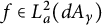
$f\in L_a^2(dA_\gamma )$
 .
Proof By Kolmogorov’s three-series theorem [Reference Durrett10, Theorem 2.5.8], we have that

4.2 Hadamard lacunary series
A sequence
$\{n_k\}_{k\geq 1}$
 of positive integers is called lacunary if
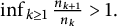
$\inf _{k\geq 1}\frac {n_{k+1}}{n_k}> 1.$
 The corresponding series
$\sum _{k=1}^{\infty }a_{n_k}z^{n_k}$
 is also called lacunary if
$\{n_k\}_{k\geq 1}$
 is.
Proposition 23 Let
$\{X_n\}_{n\geq 1}$
 be a sequence of nonzero i.i.d. random variables and
$0<s,p,q,u<\infty $
 . Let
$f(z)=\sum _{k=1}^{\infty }a_kz^{n_k}$
 , where
$\{n_k\}_{k\geq 1}$
 is a lacunary sequence.
-
(i) If $f\in H^{s,q,u}(\mathbb {D})$
and
$X_1\in L^{q}(\Omega )$
, then
$\mathcal {R}f\in H^{p,q,u}(\mathbb {D})$
a.s. -
(ii) If $\mathcal {R}f\in H^{s,q,u}(\mathbb {D})$
a.s. and
$X_1\in L^2(\Omega )$
, then
$f\in H^{p,q,u}(\mathbb {D})$
.






The proof is based on the following lemma.
Lemma 24 [Reference Jevtić, Vukotić and Arsenović15, p. 192]
A function
$f(z)=\sum _{k=1}^{\infty }a_kz^{n_k}$
 , analytic in
$\mathbb {D}$
 , where
$\{n_k\}_{k\geq 1}$
 is a lacunary sequence, belongs to
$H^{p,q,u}(\mathbb {D})$
 if and only if
$\{n_k^{-u}a_k\}$
 belongs to
$l^q$
 .
Proof of Proposition 23
(i) Since

by Lemma 24, we have
$\mathcal {R}f\in H^{p,q,u}(\mathbb {D})$
 a.s.
(ii) If
$f\notin H^{p,q,u}(\mathbb {D})$
 , that is,
$\sum _{k=1}^{\infty }|n_k^{-u}a_k|^q=\infty $
 , then

by the Paley–Zygmund inequality [Reference Li and Queffélec18, Proposition III.3, p. 23]. It follows that

Let
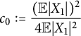
$c_0:=\displaystyle \frac {(\mathbb {E}|X_1|)^2}{4\mathbb {E}|X_1|^2}$
 ,
$c_1:=(\frac {1}{2})^q(\mathbb {E}|X_1|)^q$
 ,
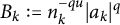
$B_k:=n_k^{-qu}|a_k|^q$
 ,
$Z_k:=n_k^{-qu}|X_k|^q|a_k|^q$
 ,
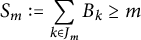
$S_m:=\displaystyle \sum _{k\in J_m}B_k\geq m$
 , and
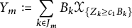
$Y_m:=\displaystyle \sum _{k\in J_m}B_k\mathcal {X}_{\{Z_k\geq c_1B_k\}}$
 , where
$J_m$
 is defined analogously to
$J_l$
 in Theorem 6. Also, one has
$0\leq Y_m\leq S_m$
 and
$\mathbb {E}Y_m^2\leq S_m^2$
 . Equation (28) reduces to

By (29),

By the Paley–Zygmund inequality again,

Since
$\sum _{m=1}^{\infty }\mathbb {P}\left (\{Y_m\geq \frac {1}{2}\mathbb {E}Y_m\}\right )=\infty $
 , we have

by the Borel–Cantelli lemma. So,

holds for infinitely many
$J_m$
 . Then
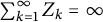
$\sum _{k=1}^{\infty }Z_k=\infty $
 a.s. Hence, by Lemma 24,

a contradiction.



